Adaptive differentiating filter: case study of PID feedback control

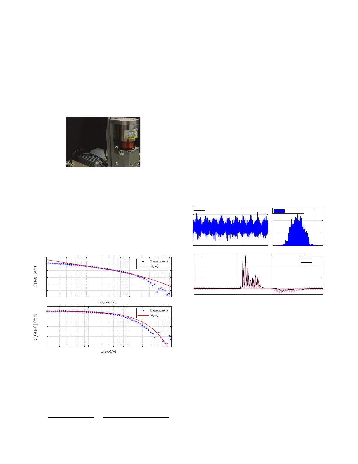
Adaptiv e differ entiating filter: case study of PID feedback contr ol Alexey Pa vlov , Mich a el Ruderman Abstract — This paper presents an adapti ve causal discrete-time filter for derivati ve estimation, exemplified by its use in estimatin g re lative velocity in a mechatronic application. The filter is based on a constrained least- squares estimator with wi n dow adaptation. It demonstrates low sensitivity to l ow-am plitud e measurem ent n oise, while preser ving a wide bandwidth f or large -amplitude changes in the pr ocess signal. Fa vorable perf ormance pro perties of the filter a re discussed and demonstrated in a practical case stu dy of PID f eedback controller and compared experimentally to a standard linear low-pass fi lter -based differentiator and a robust sliding-mode based homogeneous differentiator . I . I N T RO D U C T I O N Obtaining trustful (thus usefu l) deriv ati ve of a measured signal b e lo ngs to the central practical problem s in th e sys- tems and control the o ry and engineerin g. The so-called fixed structure (or fixed size) filters sha re the same fundam ental problem , in other words trade-off between a noise red uction and p hase la g (o r corr esponding delay) in th e o u tput sign al and its time deri vati ve(s). Po ssessing the requir e d noise filtering prope r ties and, at the same tim e, preserving faster transients o f the process sign al are the key and d emanding characteristics, for which the advanced real-time adaptive and implem entable methods are required. Especially ca usal differentiators (these vital for real- time mon itoring and con- trol tasks) face p erforma n ce lim itations with re spect to the estimate accu r acy , computatio nal and memory con sumption, and difficulties with tuning of fr ee design param eter(s). In this comm unication, we introduce a causal adap tive differentiating filter , particular ly suitable for con trol appli- cations, and dem onstrate a detailed case study of applying it in the stand ard PID feedback loop , where o nly a noisy output signal is av ailable f rom sensing. In an experimen tal real-time setting, the filter demonstrated very low sensiti vity to measurem e nt noise wh ile, same time, preser ving large bandwidth of the process signal. W ithout any claim on a m ple overview of the other w ise existing techniques and du e to the space limits, we solely ref er to few related works (with referenc e s therein) which are providin g d eeper insight into developments of causal (and also adaptive) differentiation algorithm s fo r noisy and less smooth sign a ls. An overview of num erical differentiation in noisy en vironm ent b y using algebraic approa c h es and implem entation in terms of a classical fin ite im p ulse respo nse (FIR) digital filter can b e found e.g. in [ 1]. A lecture no te o n Savitzky-Golay filter o f A. Pavlo v is with Norweg ian Univ ersity of Science and T echnology (NTNU), Trondheim, Norwa y . Email: al exey.pavlov@ntn u.no M. Ruderma n is with Univ ersity of Agder , Grimstad, Norway . E mail: michael.ruder man@uia.no ————— ——– IF AC author s manuscrip t, 2025 smoothing the data without distorting the signal tendency , by principle of local least-squar e s app roximation (s) which is also in core of our p roposed approach , can b e found in [2 ]. Also th e robust sliding- mode based (see [ 3] fo r basics) d if- ferentiator s, to one fr om which estab lished methods we make also c o mparison in this work, are the objective of intensiv e theoretical and p ractical studies in the last deca d e, cf. e.g. survey with experiments in [4 ] . An other remarkab le practical approa c h , which uses a tim e adap ti ve win dowing an d least- squares fitting, and, th us, p rovides certain motiv ation f or ou r developed solution, can be fou nd in [5]. Compared to [5], o ur approa c h separates window adaptatio n from the calculation of the signal deriv ati ve estimate, which leads to an optimal window ada p tation and highe r computation al efficiency . The rest of the paper is as f o llows. The adap ti ve d iffer - entiating filter is introd u ced in Section II b y providing th e concept, algorithms, imp le m entation steps, and pro perties. The secon d piece of the main results is given in Section III, presenting a detailed case stud y of usin g the pro posed filter in a real-time PID co ntrol applicatio n with experiments. Omitted detailed discussion (which is up to our f u ture works) is justified by the main con clusions in Section IV. I I . A D A P T I V E D I FF E R E N T I A T I N G F I L T E R ( A D F ) Consider a signal ¯ x ( t ) samp led at time instances t l = l · T s , l = 0 , 1 , . . . , w ith sampling period T s ≥ 0 : x l = ¯ x ( t l ) + w l , (1) where w l is the measurem e nt noise. It is assumed that the noise satisfies | w l | ≤ d, ∀ l ≥ 0 , (2) where d > 0 is the up p er b ound on the n oise magnitud e. The upper bou nd d is assumed to be known, e.g., from a sensor specification or can be estimated fro m prior tests. A. ADF concept At time instant t l , the outpu ts of the filter are calcu lated from the p a st measuremen ts with ind ices from the window W l ( R ) = { l − R , . . . l } , (3) for so m e R ≥ 1 , which will be specified later , using the constrained least squ ares method: ( k ∗ l , b ∗ l ) = arg min ( k , b ) ∈ R 2 , | x ( t l ) − b | ≤ δ X i ∈ W l ( R ) | x ( t i ) − k ( t i − t l ) − b | 2 , (4) where k ∗ l is the filter output provid ing an estimate of d ¯ x ( t l ) /dt and b ∗ l is the estimate of ¯ x ( t l ) . The constraint is | x ( t l ) − b | ≤ δ, (5) where δ ≥ d is a filter parameter in tr oduced to take in to account | x l − ¯ x ( t l ) | ≤ d , that follows from (1), (2 ). While fitting a linear function to the time series u sin g the least-squares meth o d is a standard appr oach, the m a in challenge is selecting th e win dow W l ( R ) . A small window size R will result in accura te following th e signa l deriv a- ti ve, yet at the cost of high sensiti vity of the deriv ati ve estimate to m easurement noise. Large R will redu ce noise sensiti vity . At the same time, f o r large R , the filter (4) will smooth ou t large/fast peaks in th e signal and, thus, lead to an und erestimation of the c o rrespon d ing ch anges in the signal de riv ati ve. Th e latter situation occurs when the signal deriv ativ e experiences large chang es over W l ( R ) . T o resolve this trade- off, we propose automatically adapt- ing the window size R based on the measurements. The window size R is selected to be the largest positiv e nu mber such that the time series (1) can b e approxim ated over W l ( R ) by a lin ear fu n ction x = k ( t − t l ) + b f or some k an d b with a given abso lu te accuracy δ : | x ( t i ) − k ( t i − t l ) − b | ≤ δ, ∀ i ∈ W l ( R ) , (6) 1 ≤ R ≤ R max . Here, δ > 0 is th e same filter parameter as in (4) an d R max is maximal win dow size introduc ed fo r a pra ctical imple- mentation. Selecting R in this way , we a void windows over which th e signal is high ly dynam ic and, thus, av oid filterin g out large peak s in th e u seful signal. At the same tim e, we keep th e window size max imal p ossible to ensure the lowest possible noise sensiti vity of the deriv ati ve estimate. Note th a t the problem of verif ying th e feasibility of (6) does not req uire an explicit calculation of the particu lar ( k , b ) . This m akes the win dow size ad aptation indepen dent of the particu lar meth o d of solving (6) and fu lly deco upled from solvin g the least squares pr oblem (4), as oppo sed to [5]. A ded ic a te d tool for verify in g the fe a sibility of (6) without finding ( k , b ) will be p r esented later in this sectio n . T o summ a rize, at each instant l ≥ 1 , the ADF filter solves the fo llowing two optimization subpro blems: • W indo w op timizatio n: find R ∗ = R ∗ ( l ) – the largest R ≤ R max such that ( 6 ) is feasible for so me ( k , b ) . • Estimates calcu la tion: for the window W l ( R ∗ ) , find the estimates o f the signal a n d its deriv ati ve by solv ing the constrained least squ ares problem (4). The set of R satisfying (6), is always non-e m pty: for R = 1 , the window W l ( R ) consists only of two points and one c an fit a linear function to these two points exactly . For th e o ptimal R = R ∗ , the solution of (4) exists and is uniqu ely define d . Thus, the filter is well-define d for all l ≥ 1 . B. ADF algorithm Sev eral features of the ADF filter allow its efficient implementatio n. Firstly , due to the linearity of (6), if th at set of ine q ualities is feasible for so me R , it is also feasible for all windows with a smaller R . In the same way , if (6) is not feasible fo r some R , it will not b e feasible for all windows with larger R . Therefor e, the largest window size R ∗ can be foun d fro m an initial guess by increasing its value while (6) remains fea sib le, or reducing its v alue u ntil (6 ) tur n s unfeasible. This is reflected in the f o llowing algo rithm: Algorithm 1: 1) l ← 0 , R ← 1 // initializatio n read x ( t 0 ) ; return ˆ dx dt ( t 0 ) = ∅ , ˆ x ( t 0 ) = x ( t 0 ) 2) while true // main loop 3) l ← l + 1 ; R ← min { R + 1 , R max } 4) read x ( t l ) 5) while (6) is not feasible fo r W l ( R ) R ← R − 1 end 6) R ∗ ← R // o ptimal R 7) calculate k ∗ l , b ∗ l from (4) fo r W l ( R ∗ ) 8) return ˆ dx dt ( t l ) = k ∗ l , ˆ x ( t l ) = b ∗ l 9) end Checking the fe a sibility of (6) in step 5) and solving th e least squares fit problem in step 7) may seem to be co mputation - ally critical for re al-time applications. Belo w , we present the efficient m ethods for real-time ADF implementation . C. T ools for efficient ADF imp lementation The following theorem allows one to check the feasibility of (6) witho ut calculating the lin e ar approx imation. Theor em 1: Inequa lity (6) is feasible if and o nly if m ≤ M , where (7) m = max i,j ∈ W | t i >t j x ( t i ) − x ( t j ) t i − t j − 2 δ t i − t j , (8) M = min i,j ∈ W | t i >t j x ( t i ) − x ( t j ) t i − t j + 2 δ t i − t j . (9) Pr o of: The proof is o mitted due to space limits and will b e provided in futur e work s. Calculation (8) and (9) can be made ef ficient by reusing the correspo nding calculation s of m and M fro m the previ- ous iteration. Notice , that all windows W l ( R ) in Algorith m 1 are obtaine d fr om the windows f rom previous iter ations by one or more of the following elementar y operatio ns: addin g a new m easurement point to an already existing window W = W l ( R ) from th e r ig ht (step 3, W = W l ( R ) → W + := W l +1 ( R + 1) ), and removing one poin t fr om the left (step 5, W l ( R ) → W − := W l ( R − 1) ). Below , we will demon strate how m and M evolve u n der these elemen tar y operations. Consider a window W := W l ( R ) . Define the vectors ¯ m ( W ) = [ m 1 , m 2 , . . . m R ] , ¯ M ( W ) = [ M 1 , M 2 , . . . M R ] of m k ( W ) = max j = l − k i = j, . . . l  x i − x j − 2 δ t i − t j  , (10) M k ( W ) = min j = l − k i = j, . . . l  x i − x j + 2 δ t i − t j  , (11) for k = 1 , . . . , R . If the vectors ¯ m ( W ) and ¯ M ( W ) are known, th en the numbe r s m an d M defined in (8) and (9) for window W can be obtained fro m m ( W ) = max[ m 1 , . . . m R ] , (12) M ( W ) = min[ M 1 , . . . M R ] . (13 ) Suppose that window vectors ¯ m ( W ) and ¯ M ( W ) are known for W = W l ( R ) . Let us d eriv e h ow they can b e calcu- lated fo r two new ad ditional wind ows: W + = W l +1 ( R + 1) and W − = W l ( R − 1) . 1) Adding a point to the right: W → W + : As follows from (10) an d the definition o f W l +1 ( R + 1) , we have m k ( W + ) = max j = l + 1 − k i = j, . . . l + 1  x i − x j − 2 δ t i − t j  = max      max j = l + 1 − k i = j, . . . l  x i − x j − 2 δ t i − t j  , (14) x l +1 − x l +1 − k − 2 δ t l +1 − t l +1 − k  , k = 1 , . . . R + 1 . Since the first eleme n t und er th e ma x function in (14) eq uals m k − 1 ( W ) , we obtain m 1 ( W + ) = x l +1 − x l − 2 δ t l +1 − t l (15) m k ( W + ) = max  m k − 1 ( W ) , x l +1 − x l +1 − k − 2 δ t l +1 − t l +1 − k  , k = 2 , . . . R + 1 . Repeating the same steps for M k ( W + ) , we o btain M 1 ( W + ) = x l +1 − x l + 2 δ t l +1 − t l (16) M k ( W + ) = min  M k − 1 ( W ) , x l +1 − x l +1 − k + 2 δ t l +1 − t l +1 − k  , k = 2 , . . . R + 1 . Eqs. (15) and (16 ) allow one to efficiently ca lc u late ¯ m ( W + ) and ¯ M ( W + ) from ¯ m ( W ) and ¯ M ( W ) . T ogether with (12) , (13) it lea ds to efficient calculation of m ( W + ) , M ( W + ) . 2) Removing a point fr om the left: W → W − : Th is case m k ( W − ) = max j = l − k i = j, . . . l  x i − x j − 2 δ t i − t j  , (17) for k = 1 , . . . R − 1 H e n ce, m k ( W − ) = m k ( W ) , k = 1 , . . . R − 1 . (18) In the sam e way , M k ( W − ) = M k ( W ) , k = 1 , . . . R − 1 . (19) Eqs. (18) and (19) allow o ne to efficiently calculate ¯ m ( W − ) and ¯ M ( W − ) from ¯ m ( W ) and ¯ M ( W ) . T og ether with (12 ), (13) it lea ds to efficient calculation of m ( W − ) , M ( W − ) . 3) Calculation of least sq uar es fit: On e can solve the constrained least-squ ares prob lem (4) u sing existing algo - rithms, e. g., av ailable in MA TLAB. Ho wever , they may not be suitable for a real-time implementa tio n on a dedicated hardware. Since (4 ) is a special case of the gen eric least squares fit problem, it allows an analytic solution presented below , which can be im plemented in a re a l-time setting. Consider win dow W = W l ( R ) . Let T := ( t l − R − t l , . . . , t l − 1 − t l , 0) ⊤ , X := ( x l − R , . . . , x l − 1 , x l ) ⊤ , τ = P R i =0 t l − i , χ = P R i =0 x l − i I := (1 , . . . , 1) ⊤ Then the solution of th e u nconstrain e d prob le m (4) is giv en by k ∗ l = X ⊤ Φ , b ∗ l = X ⊤ Ψ , where (20) Φ = T − τ R +1 I T ⊤ ( T − τ R +1 I ) , Ψ = I R + 1 − Φ τ . (21) For the constra in ed least squar es pr oblem, if | b ∗ l − x l | > δ , then the solution to the co nstrained problem (4) is given by ˜ b ∗ l = x l + sig n( b ∗ l − x l ) δ, (22) ˜ k ∗ l = X ⊤ T − ˜ b ∗ l (( R + 1 ) t l − τ ) − t l χ T ⊤ T + ( R + 1) t 2 l − 2 t l τ . (23) For applicatio ns with a fixed sampling rate, th e vectors Φ and Ψ will only d epend on the size of the w in dow R , and will no t d epend on l . This allows one to pr e-compu te th e m upfro nt, which m akes the calculation mor e efficient. D. Pr op erties of ADF filter 1) T uning a nd performance: ADF h a s two parameters: R max and δ . On e can choo se R max sufficiently large and control the filter perform ance by the main par ameter δ . Th e estimate ˆ x l of the signal provided by ADF satisfies, cf. ( 4), | x l − ˆ x l | ≤ δ. (24) Thus, for δ smaller than the noise amp litude d , th e output and its estimated deriv ati ve will reflect noise. V ery large δ leads to filtering thro ugh (4) over th e largest m oving wind ow of the size R max . T he op tim al tuning is with δ righ t above the noise amp litude d . W ith such tuning, the filter has a wide pass-b and fo r signals of sufficiently hig h amplitu des relativ e to δ a n d lo w sensiti vity to measuremen t noise w ith amplitudes below δ , that is often requ ired in applications. 2) Memory requir eme n ts: Given p arameter R max , ADF requires two array s of size 1 × R max for storing the buffer with the last R max measuremen ts and sam p les times, two arrays ¯ m and ¯ M of the size 1 × R max , as well as se veral scalar variables for real-time calculatio ns. I I I . P I D C O N T RO L C A S E S T U DY A stand ard PID co ntrol, see e.g. [6] for basics and ad- vanced discussions, is taken as a case study for ev aluating the pr o perties and practical applicability of the ab ove in tro- duced adaptive differentiating filter . Recall that any PID-type feedback regulator assumes a first-or der tim e d eriv ati ve of the outpu t value, which is (m ore than of ten) not available throug h sen sor measu rements. For an across domain s exam- ple, any motio n contro l system with PID feed back control would req uire measurem ent of th e re la tive velocity , i. e . ˙ x ( t ) , for which there is hardly any sensor technolo gy suitable for feedback. Thus, a pr actical differentiating filter, in terms of unav oidable ph ase-lag cha racteristics an d a subseq uently achiev able signal-to- n oise ratio (SNR), app ears cruc ial for effecti veness of th e PID con trol in countless app lications. A. PID feedback with symmetrical op timum PID feedback regulator, pa r ameterized by the overall con- trol g a in K p and two time co nstants – of the integrator and differentiator T i and T d respectively – can be wr itten in Lapla c e s - domain in a parallel form as, cf. e .g. [7], v ( s ) = K p  1 + 1 T i s + T d s  e ( s ) . (25) The contro l erro r is e = r − x , where x is the measu r ed system output and r is the c o ntrol reference value. In th e following, it is assumed that th e latter is at least on ce differentiable, wh ile | ˙ r | < R and the upper boun d 0 < R < ∞ is the matter of an application’ s specification. W e also note that the transfer functio n C ( s ) = v ( s ) /e ( s ) of the PID control (2 5) is stric tly speaking im proper, but the applica tio n of an (arbitrar y ) differentiating filter to determine e ( s ) s will provide additional low-pass prop erties. Thu s an d , moreover , due to a par allel conn e ction of the PID contro l (25) ther e are no issues with an impro per tr a nsfer functio n C ( s ) . 10 0 10 1 10 2 10 3 -20 0 20 40 c 10 0 10 1 10 2 10 3 -720 -630 -540 -450 -360 -270 -180 -90 Fig. 1. Sha ped loop transfer function C ( j ω ) G ( j ω ) with identifie d system plant G ( j ω ) and PID control C ( j ω ) designed by symmetrical optimum. For determining the con trol parameters K p , T i , T d > 0 , we p roceed with loop-sha p ing b y following the prin c iples of so-called symm e tr ical o ptimum [8]. The sym metrical optimum , in fr equency domain , is achieved by shaping a − 2 0 dB/decade slope aroun d the cross-over frequen cy ω c , while both cor ner frequencie s left- and righ t-hand-sid e from ω c are shaped to be appr o ximately equid istan t on the lo g arithmic scale, see Fig . 1 . W orth noting is also th at th e co rrespond ing system plant tran sfer fu n ction G ( s ) , cf. the p resent system in section III-D, is equ ally cruc ia l wh en shaping th e loop by a symm etrical optimum prin ciple. Th e determined contr ol parameters thus determine d are K p = 420 , T i = 0 . 07 , and T d = 0 . 0 3 , while it is explicitly emph asized that one and the same d esigned PID con troller (2 5) is experimentally ev aluated below with three different d ifferentiators, eac h one delivering an ˙ x ( t ) app roximation . Further we no tice th a t a constant gravity compensating term γ is also used, thoug h without affecting the design and analysis, so th at the overall control signal is u ( t ) = v ( t ) + γ . B. Linear filter ed differ entiation Direct discrete time differentiation of the measu r ed ou tput value x ( t ) is considered th e first and most intuiti ve (and also simplest) differentiation a p proach f or comp arison. For the given samp ling time T s , it lead s to a finite differences ˙ x ≈  x ( t ) − x ( t − T s )  /T s . (26) Since the measured x ( t ) contain s also som e unavoidable (parasitic) noise w ( t ) , and the sig n al-to-no ise ratio (SNR) has usually some finite value ≪ ∞ , the finite d ifference method ( 26) b ecomes m ore n o ise-sensitiv e when T s de- creases. Theref ore, an auxiliary low-pass filter (LPF) is required to let the n et sign al ˙ x ( t ) throu gh and, correspo nd- ingly , to attenuate the noise related ˙ w ( t ) with frequ encies higher th an some cutoff frequen cy ω 0 , which is the de sign parameter . In a most simple case, the LPF can b e assumed as a 2nd order critically-dam ped system with unity gain, parameteriz e d by its n atural frequen cy ω 0 . Follo wing the lines o f design ing the control system in continu ous time, cf . section I II-A, while assumin g a sufficiently low T s for an afterwards discrete-time implementa tio n, th e linear filtered differentiator ( further deno ted as LDF) is given b y LDF ( s ) = s ω 2 0  s 2 + 2 ω 0 s + ω 2 0  − 1 . (27) C. Robust fi nite-time differ en tiator One of the most wid espread robust (an d mor eover finite- time) d ifferentiato rs is the sliding-mode based one p r oposed by Le vant [9], [10] and rely ing, in its simplest form, on the so-called super-twisting based algorithm (ST A). Its re- markable feature is in sensiti vity to a bounded noise a n d the finite- tim e conv ergence to n - th time-deriv ativ e of the input signal x ( t ) , provide d the Lip schitz constant of its n -th time-derivati ve is av ailable. While in tensiv e resear ch on this class of differentiators was d r i ven in th e last two decades, we will solely denote it as robust exact differentiator (shortly RED), and u se its well estab lished par ameterization approa c h developed to a toolbo x [11]. The latter has an intuitive and straigh tforward non-r ecursive stru cture and is implementin g th e homog eneous d iscrete-time differentiator, as this was proposed in [12], while requir ing the single scaling factor κ > 0 as design parameter . W orth noting is that κ n +1 correspo n ds to the Lipschitz co nstant of th e highest deriv ativ e x ( n ) . The seco n d-ord er RED is gi ven, cf. [11], ˙ z 0 = z 1 + 3 . 1 κ   x − z 0   2 3 sign( x − z 0 ) , (28a) ˙ z 1 = z 2 + 3 . 2 κ 2   x − z 0   1 3 sign( x − z 0 ) , (28b) ˙ z 2 = 1 . 1 κ 3 sign( x − z 0 ) , (28c) and it provides z 0 ( t ) = x ( t ) , z 1 ( t ) = ˙ x ( t ) , z 2 ( t ) = ¨ x ( t ) for all t > t c , where t c is a finite conver gence time. W e explicitly notice that the second-ord er RED (and not the first-or der one) is pur posefully used in our study , in order to ob tain a smoother estimate z 1 ( t ) of th e output deriv ativ e ˙ x ( t ) . D. Experimental actua tor system 1) Har dwar e setup: The used actuator system in a labo- ratory setting is shown in Fig . 2. The translational relati ve motion with a mechanically limited disp la c e ment r ange about x ∈ [0 , . . . , 0 . 01 8 ) m is actuated by a v oice-co il- motor . The real-time contro l and data acquisition Speedgo at I/O board is runnin g at 2 kHz sampling frequ ency f s = 1 /T s . The controller o utput is the terminal v oltage u ( t ) ∈ [0 , . . . , 10] V of the voice-coil-motor, while its nominal electro-mag netic time constant (giv en by the manu factur er data-sheet) is µ = 0 . 0012 sec. The system o utput relativ e displacement x ( t ) is Fig. 2. Actuator system in laborator y setting with transla tional motion x . measured contactless b y a down placed ind uctiv e d istan ce sensor with a n ominal r epeat accu racy of ± 12 micrometer s. Such sensing lo c ation and overall hardware configur ation result in a relatively high le vel of the measu rement noise, cf. below in section III - E. Further details on the expe r imental system in use and identification can be found in [13], [ 14]. 2) FRF iden tified model: The in put-ou tput system mod e l (29) was accurately identified from the point-wise measu r ed FRF (fr equency respo n se function) as sh own in Fig . 3. Note 10 0 10 1 10 2 10 3 -140 -120 -100 -80 -60 -40 -20 10 0 10 1 10 2 10 3 -720 -540 -360 -180 0 Fig. 3. Measured and identified FRF of the system. that the to ta l m ovin g mass par a meter m is weighe d on the electron ic scales and thus known, equ ally as the giv en electro-mag netic time constant µ , cf. subsection above. Also, the no minal value of the overall a ctuator gain K m is kn own from the tech nical data-sheets of the voice-co il- motor . G = K m exp( − τ s ) s ( ms + ν )( µs + 1) = 3 . 28 exp ( − 0 . 011 s ) 0 . 0006 4 s 3 + 0 . 634 s 2 + 8 0 s . (29) The derived G ( s ) = x ( s ) /u ( s ) m odel (29) constitutes, this way , the best linear fit in f requency domain. The un certain and th us experimen tally e stimated parameters are the line a r damping ν and the time d e la y factor τ . Mor e details on the accomplished FRF based iden tification of the system can be found in [1 4]. Note that the time delay ap pears largely as not negligible, cf. phase d ia g ram in Fig. 3, and can be seen as the on e lumped delay value accumu lated f rom all co n verters, hardware chan n els of data pro c essing, and a m plifiers in the loop. Fur th er recall th a t the tran sf e r function ( 29) serves as a basis for symmetric a l op timum tu ning of the PID controller under examination , cf. section III-A. E. Comparison of three differ entiato rs The ADF is p a r ameterized by taking into acco unt the CPU capacities of the control bo a rd with hard real-tim e co nstraints and an estimate of the upper boun d on the measur ement no ise d , c f . section II. An example of the m e asured x ( t ) at zero control value is shown in Fig. 4 (a), in cluding its d istribution histogram. Allowing f or the single impulse-shap e o utliers, the set parame te r is δ = 0 . 0001 m, while R max = 140 for keeping the r e al-time d a ta processing m anageable and, therefor e, to av oid a CPU overrun durin g the execution. The L D F is param eterized by ω 0 = 600 r ad/sec. Note that 0 1 2 3 t (s) -1.5 -1 -0.5 0 0.5 1 x (m) 10 -4 (a) time series -0.0001 0 0.0001 x (m) 0 distribution 0.8 1 1.2 1.4 t (s) 0 0.2 0.4 0.6 dx/dt (m/sec) (b) LDF ADF Fig. 4. Measure d noisy output and its distrib ution at the idle state ( u = 0 ) in (a), and exe mplary ˙ x ( t ) estimate by means of LDF and ADF in (b). with respe c t to the designed PID controller, cf. section III- A, such low-pass filter ( applied for ob taining ˙ x ( t ) estimate only) does not significantly chan g e the shap ed loop transfer characteristics. Solely the othe r wise sufficient phase margin is reduced by less than 5 deg, c f. Fig. 1 . An exemplary estimate o f the o utput veloc ity , obtained by m eans o f the designed LDF a nd ADF , are shown op posite to e a ch oth e r in Fig. 4 (b) fo r th e measured x ( t ) d uring the c ontrolled step response, cf. below . Fina lly , th e RED is paramete r ized by setting κ = 8 , that is experimen tally tun ed as provided in [14] o n an up-ch irp signal excitation respon se within one decade (e.g . between 8 rad/sec a n d 80 rad/sec) . For the sake of a better traceability , the numerica lly determined FRFs of all three differentiators are shown for two and a half decad es in Fig. 5, oppo sed to each other and to an exact differentiation , i.e. | j ω | . Note that wa ves in the shape at lower f requencie s are associated with chirp - signal used for a smooth inp ut. Ther efore, it allows fo r an only quasi-steady- state frequency consideration, especially in the fist dec a de. Apart from that, one can recog nize tha t all three differentiators provide an expected 20 dB/dec increase over the total fr e q uency rang e of interest. T o no tice is that the RED break s down ar ound ω = 100 rad/sec, – a band width for which it was designed b y assigning the scaling factor κ . 10 0 10 1 10 2 (rad/sec) 0 10 20 30 40 50 | output / input | (dB) |j | exact RED LDF ADF Fig. 5. Numerica lly determine d FRF of three diffe rentiat ors. The designed PID control (cf. sectio n III-A) is experimen- tally ev aluated with thr e e different differentiators, LPF , ADF , and RED, o nce on a step and once on a slope ref erence, as shown in Fig. 6. All th ree differentiation schemes lead to 1 1.2 1.4 1.6 1.8 2 t (s) 0 0.005 0.01 0.015 x (m) (a) LDF ADF RED reference 1 1.2 1.4 1.6 1.8 2 t (s) 0 2 4 6 u (V) (b) LDF ADF RED 1 2 3 4 5 6 t (s) 0 0.005 0.01 0.015 x (m) (c) LDF ADF RED reference 1 2 3 4 5 6 t (s) 1 2 3 u (V) (d) LDF RED ADF Fig. 6. Measure d PID response (with L DF , AD F , RED) of output and control val ues: (a), (b) to step reference and (c), (d) to slope refere nce. a r elati vely similar contro l respon se, while ADF p rovides a slightly lower overshoot in case of the step re sp onse. Also to notice is a time delay , cf. τ in section III-D.2, an d a slow settling of the optimal PID co ntrol, cf. Fig. 6 (a), due to the non linear Coulom b -type friction, see [ 15] for details. An essential a dvantage of u sing ADF differentiator becomes evident by in specting u ( t ) con trol values, cf. Fig. 6 (b) and (d ). While being in princip le unif orm, th e higher oscillatory contro l patterns (and so en ergy con sumption an d system load ing) are clearly with LDF and RED du e to richer frequen cy compo nents o f ˙ x ( t ) estimate, cf. also Fig. 4 (b) . I V . C O N C L U D I N G S TA T E M E N T S A novel causal discrete-time filter based on a constrained least-squares estimator with wind ow adaptation was pr o - posed for differentiating no isy p r ocess m easurements. It shows low sen sitivity to th e measu rement n oise while p re- serving large amplitude and high-dyn amic chan ges in the process sign al. The filter is real-time capable and shows excellent perf o rmance in differential feed back con trol action , ev aluated and compar ed on a re a l phy sical motion control application. More detailed an alysis of the filter sensitivity and conv ergence p roperties, tran sfer characteristics, and op timal tuning are su b ject of our up coming works in prog ress. R E F E R E N C E S [1] M. Mboup, C. Join, and M. Fliess, “Numerical differe ntiati on with annihil ators in noisy en vironme nt, ” Numerical algorithms , vol. 50, no. 4, pp. 439–467, 2009. [2] R. W . Schafer , “What is a Savitzk y-Golay filter? [lectu re notes], ” IEEE Signal Proce ssing Ma gazine , vol . 28, no. 4, pp. 111–117, 2011. [3] V . Utkin, Slidin g modes in contr ol and optimizati on . Springer , 1992. [4] M. R. Mojall izadeh, B. Brogliat o, A. Polyako v , S. Selvara jan, L. Michel, F . Plestan, M. Ghanes, J.-P . Barbot, and Y . Aoustin, “ A s ur- ve y on the discrete -time differe ntiator s in closed-lo op control systems: Experiments on an elect ro-pneumati c system, ” Contr ol Engineering Practic e , vol. 136, p. 105546, 2023. [5] F . Janabi-Sha rifi, V . Hayward, and C.-S. Chen, “Discrete-ti me adapti ve windo wing for velo city estimation, ” IEEE Tr ansactio ns on contr ol systems techno logy , vol. 8, no. 6, pp. 1003–1009, 2000. [6] K. Astr ¨ om and T . H ¨ agglund, Advanced PID Contr ol , ser . Interna tional Society of A utomation. Wi ley , 2005. [7] G. Franklin, J. Powe ll, and A. E m ami-Naei ni, F eedback Contr ol of Dynamic Systems , eight ed. Pea rson, 2019. [8] C. Kessl er , “Das symm etrisc he Optimum, T eile I und II, ” at- Automat isierungstec hnik , vol. 6, pp. 395–400, 432–436, 1958. [9] A. Lev ant, “Robu st exact differe ntiati on via sliding mode technique, ” Automat ica , vol . 34, no. 3, pp. 379–384, 1998. [10] A. Lev ant, “Higher-o rder sliding modes, dif ferenti ation and output- feedbac k control, ” Int. J. of Con. , vol . 76, pp. 924–941, 2003. [11] M. Reichha rtinger , S. S purgeon, M. Forstinger , and M. Wip fler , “ A robust exact dif ferent iator toolbox for Matlab®/Si mulink®, ” IF AC- P apersOnLine , vol. 50, no. 1, pp. 1711–1716 , 2017. [12] M. Li vne and A. L e v ant, “Proper discretiza tion of homogeneous dif ferenti ators, ” Automat ica , vol . 50, no. 8, pp. 2007–2014, 2014. [13] M. Ruderman, “Motion control with optimal nonlinear damping: from theory to e xperiment, ” Con. Eng. Prac. , vol. 127, 2022. [14] M. Ruderma n, J. Reger , B. Calmbach, and L. Fridman, “Sensiti vity analysi s and experiment al ev alua tion of P ID-like continuous slidin g mode control, ” Int. J. of Rob . and Nonlin. Con. , vol. appeari ng, 2026. [15] M. Ruderman, “On con ver gence analysis of feedback control with inte gral action and discontinuo us relay perturbat ion, ” Communications in Nonlin. Scien ce and Num. Simula tion , vol. 145, 2025.