Time-varying System Identification of Bedform Dynamics Using Modal Decomposition

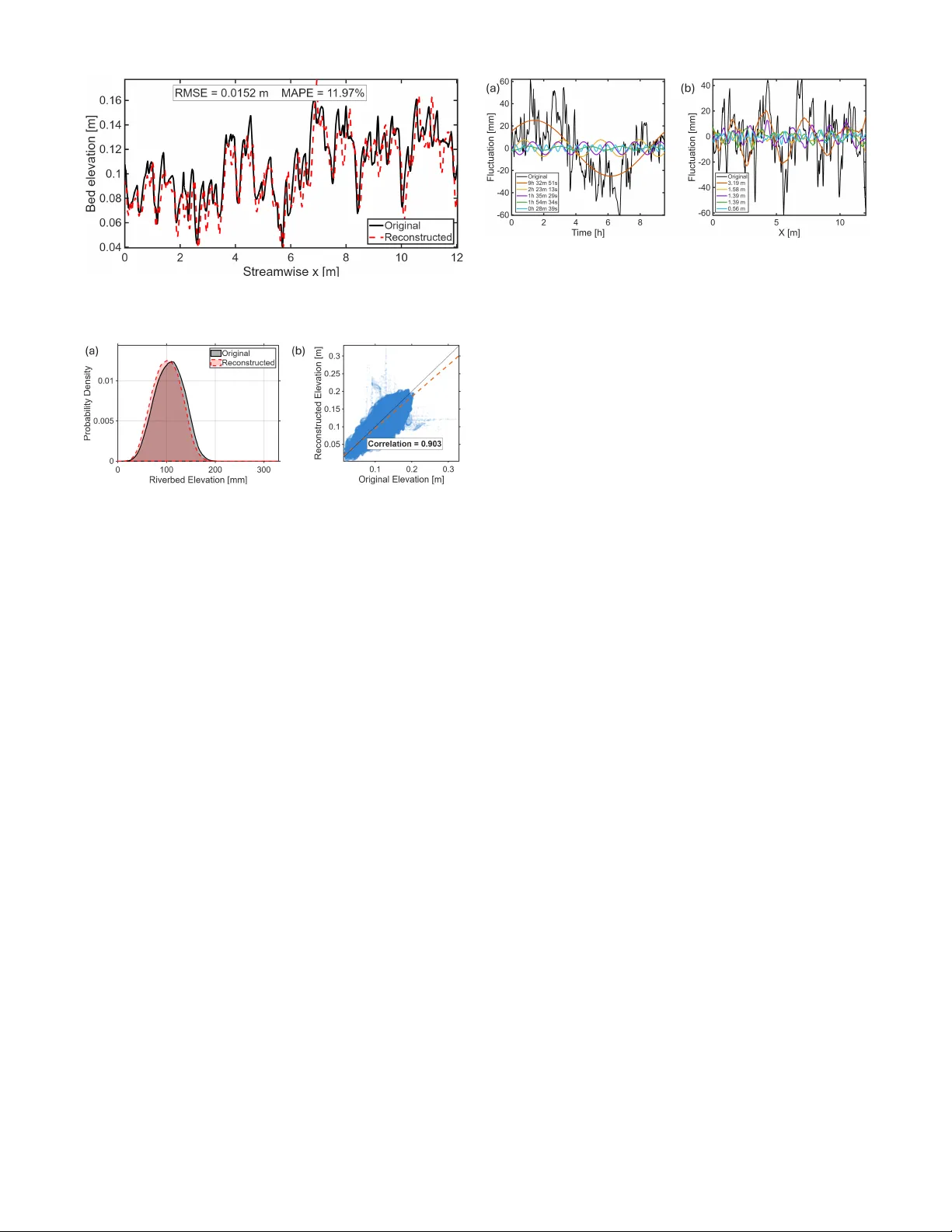
T ime-varying System Identification of Bedform Dynamics Using Modal Decomposition Shakib Mustav ee (Member IEEE) 1 , Arvind Singh, and Shaurya Agarwal (Senior Member IEEE) 2 Abstract — Measuring sediment transport in riverbeds has long been a challenging resear ch problem in geomor phology and river engineering. T raditional approaches rely on direct measurements using sediment samplers. Although such mea- surements ar e often considered ground truth, they ar e intrusive, labor -intensive, and pr one to large variability . As an alternative, sediment flux can be inferred indirectly from the kinematics of migrating bedforms and temporal changes in bathymetry . While such approaches ar e helpful, bedf orm dynamics are nonlinear and multiscale, making it difficult to determine the contributions of different scales to the overall sediment flux. Fourier decomposition has been applied to examine bedform scaling, but it treats spatial and temporal variability separately . In this work, we introduce Dynamic Mode Decomposition (DMD) as a data-driven framework f or analyzing riverbed evolution. By incorporating this representation into the Exner equation, we establish a link between modal dynamics and net sediment flux. This formulation provides a surrogate measure for scale-dependent sediment transport, enabling new insights into multiscale bedform-dri ven sediment flux in fluvial channels. I . I N T RO D U C T I O N Accurately modeling and predicting sediment transport in fluvial en vironments remains a fundamental challenge in geomorphology and ri ver engineering. Fluvial channels act as primary conduits for both water and sediment [1], [2]. The continuous processes of erosion and deposition shape Earth’ s surface, influence ecological div ersity , and affect human activities such as navig ation, flood control, and infrastructure dev elopment [3]. Since sediment transport underpins both the morphology and function of channel systems, reliable approaches for its quantification are of critical importance. T raditionally , sediment transport has been measured di- rectly using devices such as sediment traps or Helley–Smith samplers, which capture material moving along the bed ov er a specified interval [4]–[7]. While often regarded as ground truth, these methods are labor-intensi ve, intrusi ve, and highly sensitiv e to deployment conditions. Reported measurements vary substantially in space and time, in addition to fac- tors such as sampler orientation, mesh size, sediment grain distribution, and the hydrodynamic disturbance created by *A. Singh acknowledges partial support from the U.S. National Science Foundation under Grant EAR-2342936. 1 Shakib Mustav ee is a Post-doc with the Department of Civil, Environ- mental & Construction Engineering, Univ ersity of Central Florida, Orlando, Florida. shakib.mustavee@ucf.edu 2 Arvind Singh is an Associate Professor with the Department of Civil, En vironmental & Construction Engineering, University of Central Florida, Orlando, Florida. arvind.singh@ucf.edu 2 Shaurya Agarwal is an Associate Professor with the Department of Civil, En vironmental & Construction Engineering, University of Central Florida, Orlando, Florida. shaurya.agarwal@ucf.edu the device itself. As a result, direct sampling is not only time-consuming but also limited in accuracy and duration, making it insuf ficient for resolving the dynamics of sediment flux in natural channels. Gi ven these limitations, researchers hav e increasingly turned to indirect approaches. One widely adopted method is to infer sediment flux from the kinematics of migrating bedforms and from temporal changes in channel bathymetry (see for details [1], [8], [9]). Bedforms act as signatures of sediment motion. Their characteristics, such as amplitude, wav elength, and migration velocity , can provide indirect estimates of volumetric sediment flux [10]. The volumetric sediment flux, q s , represents the rate at which sediment volume passes per unit channel width. Estimating q s is central to quantifying bedload transport. Howe v er , bed- form dynamics are inherently nonlinear and strongly scale dependent [11]. Bedforms of dif ferent sizes coexist, migrate at distinct velocities, and interact through feedbacks among morphology , shear stress, and transport rate [1], [9], [12]. This multiscale v ariability makes it difficult to determine the relativ e contrib utions of different bedform scales to the overall sediment flux, which remains an open research question. Previous studies hav e used Fourier decomposition of bed elev ation fields to examine scaling behavior and the role of different bedform sizes in sediment transport [13]. These analyses showed that small, fast-migrating secondary bedforms can significantly contribute to flux and driv e the propagation of larger , slower bedforms. While Fourier meth- ods provide valuable spectral information, they treat spatial and temporal variations separately . Dynamic Mode Decomposition (DMD) has emerged as a widely used tool in fluid mechanics and data-driv en modeling, valued for its ability to extract coherent spatio- temporal patterns and provide reduced-order representations of complex flow fields [14]–[16]. In this work, we propose a novel framework based on DMD for characterizing the scale dependence of sediment transport analysis. DMD de- composes the ev olution of bed elev ation into spatio-temporal modes, each representing a coherent pattern with an asso- ciated growth/decay rate and frequency . This makes DMD particularly well-suited for the “tall-and-skinny” structure of riv erbed elev ation datasets, where many spatial samples are collected over relatively short time records [17]. By substi- tuting the DMD-based linear approximation of bed elev ation dynamics into the Exner equation and integrating across space, we establish a connection between DMD modes and net sediment flux. Contributions: The contributions of this article are as fol- lows: Fig. 1. Riv erbed topography visualization. (a) Illustrates 2D topography at a specific time. (b) Spatial bed elev ation profile along a selected transect (shown in red line in Figure 1(a)). (c) Spatio-temporal ev olution of the riv erbed topography . The figure also describes the dimensions of the data. (d) T emporal bed elev ation profile along a selected point. • The paper studies the spatio-temporal coherent structure of the riverbed elev ation using DMD. • It deriv es a mathematical connection between sediment flux and spatio-temporal modes of riverbed elev ation computed from DMD. I I . D AT A D E S C R I P T I O N The dataset analyzed in this study originates from large- scale flume experiments conducted at the St. Anthony Falls Laboratory (SAFL) Main Channel. The flume is 85 m long and horizontally 2 . 75 m wide and is equipped with discharge regulation and sediment recirculation systems to maintain morphodynamic equilibrium during experiments [2]. The spatio-temporal bed ev olution was measured along the chan- nel centerline using a submerged laser scanning de vice mounted on an automated cart. The dataset consists of three-dimensional arrays of bed ele vation change, denoted as η ( x, y , t ) , where t represents the acquisition time in seconds, x the streamwise locations, and y the spanwise locations. Formally , η ( x, y , t ) ∈ R N x × N y × N t , where N x , N y , and N t correspond to the number of streamwise, spanwise, and temporal indices, respectiv ely . Figure 1 e xplains the bed elev ation data. Figure 1 (a) illustrates the topography at a giv en moment. In the stream direction, the bed is 12 m long and 0 . 5 m wide. The elev ation of the bed is limited between 0 to 0 . 329 m . There are 3008 points in the stream direction ( N x = 3008) and there are 126 points in the span direction ( N y = 126 ). Figure 1 (b) shows the elev ation of the river bed along a transect. Figure 1(c) shows the temporal ev olution of the topography by representing the three-dimensional bed elev ation in Figure 1(a) as a two-dimensional heat map, which also illustrates the dimensions of the spatio-temporal data. Figure 1 (d) shows the temporal ev olution of a point at the middle of the channel on a transect. The data was recorded for 9 . 71 hours at a resolution of approximately 2 min, which corresponds to 300 time snapshots. This high- resolution spatio-temporal record of channel bed morphology provides an ideal basis for applying dynamic mode decom- position (DMD) to inv estigate the coherent structures and temporal dynamics of riverbed e volution. I I I . D M D F R A M E W O R K F O R B E D E L E V AT I O N A. F ormulation of DMD for Bed-Elevation Fields DMD is a data-dri ven technique that extracts coherent spatio-temporal patterns from data by decomposing it into modes and complex eigen v alues. Each mode represents a spatial structure, while each eigen value characterizes the tem- poral behavior through a growth/decay rate and oscillation frequency [17]. In practice, DMD assumes that consecuti ve snapshots of the system satisfy an approximate linear evolu- tion of the form X ′ = AX . Here, X = [ x 1 , x 2 , . . . , x m − 1 ] and X ′ = [ x 2 , x 3 , . . . , x m ] are snapshot matrices constructed from sequential measurements of the system state, where each column x k represents a v ectorized snapshot of the spatial field at time t k . The operator A is an unkno wn linear mapping that advances the state from one snapshot to the next. DMD estimates this operator directly from data and computes its eigenv alues and eigenv ectors to obtain the dominant dynamical modes. This procedure yields a reduced- order linear representation of the system dynamics, which can often be interpreted as a finite-dimensional approxima- tion of the Koopman operator [18], [19]. W e apply DMD to analyze the temporal evolu- tion of ri verbed topography described in Section II. First, we consider a sequence of bed-elev ation fields { η 1 ( x, y ) , η 2 ( x, y ) , . . . , η p ( x, y ) } measured on a Cartesian grid with m rows and n columns measured at discrete times t 1 , . . . , t p . Each snapshot can be written as: η k ≡ η k ( x, y ) ∈ R m × n , ∀ k = 1 , . . . , p. Figure 2 sho ws how the two-dimensional snapshot is vectorized by stacking each row using the vec( · ) operator: h k = vec  η k  ∈ R mn , k = 1 , . . . , p. By arranging the vectorized snapshots into a single ma- trix, we get the spatio-temporal matrix H , where, H =  h 1 , h 2 , . . . , h p  ∈ R mn × p . Here, m × n denotes the size of the spatio-temporal matrix while mn is the length of each vectorized snapshot, and p denotes the number of snapshots. W e create two metrices, H 1 and its time shifted version H 2 from H by choosing the first q + 1 number of snapshots: H 1 =  h 1 , h 2 , . . . , h q  and H 2 =  h 2 , h 3 , . . . , h q +1  . where, H 1 , H 2 ∈ R mn × q . W e assume a linear map A such that H 2 ≈ A H 1 = ⇒ A ≈ H 2 H † 1 (1) Here, A ∈ R mn × mn and H † 1 is the Moore-Penrose pseudo- in v erse of H 1 . Directly solving for A is computationally Fig. 2. Schematic showing how a two-dimensional bed elev ation snapshot is stacked into a one-dimensional column vector for constructing the DMD data matrix. expensi v e due to the high-dimensionality of the spatio- temporal matrices. DMD can tackle this problem by using the singular value decomposition (SVD) of H 1 [17]. By taking SVD we can write H 1 = U Σ V ∗ . Here, U ∈ R mn × q , Σ ∈ R q × q , V ∈ R q × mn , . Consequently , H † 1 = ( U Σ V ∗ ) † = V Σ − 1 U ∗ . Using the relation in Equation 1 a least-squares estimate of A can be written as: A ≈ H 2 H † 1 = H 2 V Σ − 1 U ∗ . W e can further reduce the dimensionality by truncating smaller ranks and keeping the r largest singular v alues. Projecting A onto the r -dimensional subspace spanned by the columns of U yields the reduced operator ˜ A = U ∗ r AU r = U ∗ r H 2 V r Σ − 1 ∈ R r × r . W e compute the eigen decomposition of the reduced operator: ˜ AW = W Λ , Λ = diag( λ 1 , . . . , λ r ) , W ∈ C r × r The DMD modes in the full state space are obtained as Φ = H 2 V Σ − 1 W ∈ C mn × r so that the k -th DMD mode ϕ k is the k -th column of Φ and can be un-vectorized to the spatial field ϕ k ( x, y ) = v ec − 1 ( ϕ k ) ∈ C m × n . One can conv ert discrete eigen v alues ( λ k ) to continuous-time eigenv alues ( ( ω k ) ) as follows: ω k = ln( λ k ) ∆ t (2) where ∆ t is the sampling interv al. W e collect all the eigen v alues into Ω = diag ( ω 1 , . . . , ω r ) . W e define the modal amplitude vector α ∈ C r from the initial snapshot. If no mean-remov al is used, a common choice is α = Φ † h 1 , Fig. 3. Semicircular distribution of DMD eigenspectra estimated from spatio-temporal bed elevation data. Due to symmetry , only the upper half of the unit circle is shown. The semicircle is partitioned into four regions based on period ranges. Here, N denotes the number of eigen v alues within each region. Eigenv alues inside the unit semicircle are annotated with their individual periods, while those on the unit semicircle are color-coded according to period. where Φ † is the Moore–Penrose pseudo-in v erse of Φ . Then the reconstructed vectorized state at continuous time t is ˆ h ( t ) = Φ  e Ω t α  (continuous-time form) or , in discrete-time at snapshot index j (with t j = ( j − 1)∆ t ), ˆ h j = Φ Λ j − 1 α (discrete-time form). Finally , we reshape the vector back to the spatial field: b η ( x, y , t ) = vec − 1  ˆ h ( t )  ∈ R m × n . It is a common practice in DMD analysis to remov e the temporal mean from the data to focus on the fluctuations. Removing the mean elev ation we get, ¯ η = 1 K K X k =1 η k ( x, y ) , ¯ h = vec( ¯ η ) ∈ R mn , and form fluctuation snapshots ˜ h k = h k − ¯ h, ˜ H 1 = [ ˜ h 1 , . . . , ˜ h K − 1 ] , ˜ H 2 = [ ˜ h 2 , . . . , ˜ h K ] . Apply the SVD and DMD steps abov e to ˜ H 1 , ˜ H 2 to ob- tain fluctuation modes ˜ Φ , eigen v alues ˜ Λ , and amplitudes ˜ α (computed for example by ˜ α = ˜ Φ † ˜ h 1 ). The full-field reconstruction then adds the mean back: b h ( t ) = ¯ h + ˜ Φ e Ω t ˜ α, or equiv alently at discrete snapshot j , b h j = ¯ h + ˜ Φ ˜ Λ j − 1 ˜ α. Finally , b η ( x, y , t j ) = vec − 1  b h j  . (3) Here, ϕ k ( x, y ) encodes coherent spatial patterns, ω k de- termines their temporal evolution, and α k sets their relative amplitudes. Fig. 4. Comparison of real river bed elevation and that of DMD reconstructed snapshot at a transect. Fig. 5. (a) Comparison of the probability distribution function between the real riv er bed elevation and that of the DMD reconstructed. (b) Scatter plot correlation between the original riverbed elevation and that of the DMD reconstructed. B. DMD Results W e ha v e applied DMD on the bed elev ation dynamics described in Section II. The dataset has 300 snapshots. W e hav e selected 98% of the data and took full rank in SVD. It has been observed that the elev ation dynamics are sensitiv e to rank reduction. Discarding ranks can significantly distort the eigenspectrum by introducing spurious values. Since DMD attempts to preserve the Frobenius norm of the A matrix, it can introduce spurious eigen v alues. This significantly dete- riorates the reconstruction performance. At the same time, it distorts the eigenspectra, which impairs accurate system identification. Therefore, we selected full rank. In the full rank SVD, the maximum number of possible eigenv alue is 294 ( 98% of 300 snapshots). Since each eigen v alue has a complex conjugate, we obtained 147 different frequencies (time period, T = 1 /f ) from the analysis. Figure 3 shows the DMD spectra. It also shows the periods associated with identified DMD eigen v alues. The periods were estimated using Equation 2. The size of the dots representing the eigen v alue is proportional to the DMD power associated with the mode. This helps identify the strength of the mode and its temporal period. In general, DMD eigen v alues are plotted on a unit circle. Since DMD eigen v alues exhibit symmetric beha vior along x-axis, for brevity we plot only the upper half. W e divide the semicircle into four regions based on periods. From left to right, along the semicircle, frequency decreases and time period increases. The di vided regions are shown using separate en v elopes. The figure illustrates the range of time periods in Fig. 6. (a) Elev ation fluctuation and dominant top fiv e DMD modes that contribute most to the sediment transportation are shown at a fixed point over time. (b) Elev ation fluctuation and the dominant top fiv e DMD modes that contribute most to sediment transportation are shown at a fixed instant across the mid-transect. each en velope and the number of eigenv alues that fall inside the en velope. Here, if any eigen v alue ( λ ) varies by less than 1% , i.e., 0 . 99 < | λ | < 1 . 01 , we consider it to lie on the unit circle. Such an eigenv alue is associated with neither growth nor decay . In other words, it is considered persistent. On the other hand, eigen v alues that lie within the unit circle are shown with periods associated with them. These eigen v alues hav e relativ ely larger DMD po wer . Most of these eigenv alues are associated with modes shorter than 10 minutes, indicating a fast-migrating and temporally decaying component of the bedform. In total, there are 12 eigenv alues inside the unit circle, while 135 eigen v alues lie on or outside the unit circle. The range 3 . 90 − 6 min contains the majority of the periods ( N = 47 ), while only 9 eigen v alues have periods longer than 1 hour. This indicates that bedform migration dynamics are primarily dominated by shorter periods or high-frequency components. T o a void clutter, we did not annotate individual periods on and outside the unit circle. Instead, the periods are represented using a color scale. Figure 4 shows the reconstructed bed elev ation at y = 63 for the 150th time snapshot. The MAPE (mean absolute per- centage error) estimated for that snapshot is 11 . 97% , showing the reconstruction accuracy of DMD. The figure shows that DMD is capable of visually reconstructing the bed elev ation. The reconstruction was done using Equation 3. T o examine the overall reconstruction performance, we estimated statis- tical measures of the reconstructed dynamics by computing the probability distribution function (PDF) and scatter plot. Figure 5(a) compares the original PDF and reconstructed PDF . It shows that the reconstructed PDF almost overlaps the original. Figure 5(b) shows the correlation between the original and the reconstructed ele v ation dynamics. Each point in the correlation signifies one point η k ( x, t ) of the bed elev ation field at a particular instant. The correlation score is 0 . 9 , indicating the identified eigenv alues can accurately reconstruct the original dynamics. This is important in the sense that it ensures the system identification is justifiable. Figure 6(a) shows the evolution of selected DMD modes at a particular point. The point is located at the center of the channel. The figure shows temporal evolution of elev ation at that point. The black line represents the fluctuation of original elev ation, while the colored lines sho w the tem- poral ev olution of DMD modes associated with the point. Note that, in DMD, the mean is subtracted from the data. Therefore, DMD modes are computed from the fluctuations and compared with fluctuations rather than the raw ele v ation. Figure 6(b) characterizes the spatial behavior of the selected modes. Here we show the spatial component of the modes along one transect ( y = 63 ) at 150 th snapshot. The figure also illustrates the wavelengths associated with them. Note that the legend in Figure 6 (a) and Figure 6 (b) follows the same order . I V . L I N K I N G D M D A N D S E D I M E N T F L U X V I A T H E E X N E R E Q UA T I O N W e begin with the two-dimensional Exner equation, which represents mass balance in sediment [16], [20], [21]: (1 − λ p ) ∂ η ∂ t + ∇ ·  q s = 0 (4) where η ( x, y , t ) is the bed elev ation, λ p is the bed porosity , and  q s = ( q s,x , q s,y ) is the volumetric sediment flux vector . From DMD analysis in Section III, we obtain a linear , data-driv en approximation of the temporal evolution of the topography . In continuous-time form we write ∂ η ∂ t ≈ Lη (5) where L denotes the (linear) generator associated with the DMD model. In discrete time, DMD yields a matrix A with eigenpairs Aϕ k = λ k ϕ k ; the corresponding continuous-time generator is related by L = 1 ∆ t log( A ) , so that Lϕ k = ω k ϕ k with ω k = log( λ k ) / ∆ t . Substituting (5) into (4) yields (1 − λ p ) Lη + ∇ ·  q s = 0 = ⇒ ∇ ·  q s = − (1 − λ p ) Lη . (6) T o relate the DMD representation of η to net streamwise flux through a cross-section at a fixed y , we integrate (6) in x from x min to x max : Z x max x min ∇ ·  q s ( x, y , t ) dx = − (1 − λ p ) Z x max x min ( Lη )( x, y , t ) dx. (7) The left-hand side of the Exner equation can be written using the 2D diver gence as: Z x max x min ∇ ·  q s ( x, y , t ) dx = Z x max x min  ∂ q s,x ∂ x + ∂ q s,y ∂ y  dx = ∂ ∂ x  Z x max x min q s,x dx  + ∂ ∂ y  Z x max x min q s,y dx  = q net s,x ( y , t ) + ∂ ∂ y  Z x max x min q s,y dx  . (8) W e have defined the net streamwise flux through the transect as: q net s,x ( y , t ) := q s,x ( x max , y , t ) − q s,x ( x min , y , t ) W e obtain from Equation 8 and Equation 7 q net s,x ( y , t )+ ∂ ∂ y  Z x max x min q s,y dx  = − (1 − λ p ) Z x max x min ( Lη ) dx. (9) Fig. 7. Cumulativ e contribution of individual modes to total sediment transportation; the slo west 7 modes account for 50.9%, the fastest 120 modes contribute 25.7%, and all 147 modes explain 100% of transport. Since streamwise transport dominates and lateral flux variations are negligible, the ∂ y term is commonly dropped. This yields the leading-order relation q net s,x ( y , t ) = − (1 − λ p ) Z x max x min ( Lη ) dx. (10) W e can e xpress the reconstructed bed elev ation as a superposition of DMD modes, η ( x, y , t ) ≈ X k α k ϕ k ( x, y ) e ω k t where { ϕ k } are (continuous-time) DMD modes, α k are initial amplitudes, and ω k are the associated continuous growth rates (units [ T ] − 1 ). Under the assumptions that (i) L is linear and (ii) commuting L and the x -integral is permissible, the right-hand side of (9) becomes q net s,x ( y , t ) ≈ − (1 − λ p ) Z x max x min ( Lη ) dx (11) ≈ − (1 − λ p ) X k α k e ω k t Z x max x min Lϕ k ( x, y ) dx ≈ − (1 − λ p ) X k α k e ω k t ω k Z x max x min ϕ k ( x, y ) dx (12) Here, we used the eigen v alue relation Lϕ k = ω k ϕ k . Equation (12) shows that a weighted sum ov er DMD modes giv es the net streamwise sediment flux through a transect. Each mode contributes in proportion to its integrated spatial mode shape over the transect, its modal amplitude, and its growth/decay rate ω k . W e hav e assumed that cross-stream transport and its lateral gradient are negligible at the transect of interest. V . D I S C U S S I O N A N D I M P L I C A T I O N S In this section, we ev aluate the implications of the math- ematical deri vation in Equation 12. The goal is to ver - ify whether the surrogate measure of sediment flux es- timated from DMD modes is consistent with the litera- ture. By discarding the summation sign in Equation 12, we can write the contrib ution of each DMD mode ( ϕ k ) to the net sediment transport as q k s,x ( y , t, ϕ k ) = − (1 − λ p ) α k e ω k t ω k  R x max x min ϕ k ( x, y ) dx  . Here, q k s,x ( y , t, ϕ k ) sig- nifies the indi vidual modal contribution to the net sediment flux, allowing the net flux to be decomposed into multi- ple spatial and temporal scales. The speed associated with each mode at a transect was estimated by computing its wa velength using spatial Fourier and Hilbert analysis, then multiplying it by the frequency obtained from the DMD eigen v alues. The modes shown in Figure 6 were selected based on their contribution to sediment transport. The figure shows that slo wer modes contribute most individually , as 4 of the 5 modes depicted hav e a period longer than 1 hour. W e sort the modes based on their speed and compute cumulative contributions by summing the sorted percentile contributions from the fastest to the slowest mode. This provides a clear visualization of ho w a small subset of modes dominates total sediment transport. Figure 7 presents the cumulative contrib ution of individual modes to net sediment transport. The analysis sho ws that just the 7 slowest modes account for 50 . 9% of the total transport, while the remaining 140 modes collectively contribute the other half. Moreover , the fastest 120 modes, although numer- ous, contribute only 25 . 7% in total. This indicates that sedi- ment transport is dominated by a small number of slow , long- wa velength modes, whereas faster , short-wav elength modes provide a distributed but comparatively smaller contribution. Such behavior is consistent with recent studies sho wing that the spectral contribution of bedforms to sediment flux decreases with increasing frequency following a po wer-la w scaling q s ( f ) ∝ f − 0 . 6 [1], [2]. Because low-frequenc y components correspond to large-scale, slowly migrating bed- forms, this relationship implies that a small number of slow modes can carry a disproportionately large fraction of the sediment transport. In contrast, higher-frequency modes as- sociated with smaller bedforms contribute more modestly de- spite their larger number . Unlike purely spectral approaches, the present DMD-based framew ork directly links sediment transport to dynamically e volving spatio-temporal modes of riv erbed ev olution, allowing the contribution of each mode to the net transport to be quantified explicitly . V I . C O N C L U S I O N In this paper , we present a novel data-driv en framework for characterizing spatiotemporal mode-dependent sediment transport from ri verbed topography . By substituting DMD modes of bed elev ation into the Exner equation, we estab- lish a physics-informed link between spatio-temporal modes and net sediment flux. Our analysis shows that the largest contributions to sediment transport come from slow , long- wa velength modes, while faster , small-w av elength modes, although individually smaller , are numerous and collectiv ely influence transport dynamics. The analysis further re veals that persistent modes, characterized by DMD eigen v alues on the unit circle, act as the primary carriers of the bulk of the sediment flux. Thus, the proposed frame work provides a non-intrusiv e surrogate for measuring sediment flux, offering new insights into the multiscale structure of bedform-driv en transport. Future work will focus on extending the method- ology to characterize sediment transport under different flow and channel conditions. R E F E R E N C E S [1] J. Lee, A. Singh, and M. Guala, “On the scaling and growth limit of fluvial dunes, ” Journal of Geophysical Resear ch: Earth Surface , vol. 128, no. 6, p. e2022JF006955, 2023. [2] ——, “Reconstructing sediment transport by migrating bedforms in the physical and spectral domains, ” W ater Resources Resear c h , vol. 58, no. 7, p. e2022WR031934, 2022. [3] S. W ang, B. Fu, S. Piao, Y . L ¨ u, P . Ciais, X. Feng, and Y . W ang, “Reduced sediment transport in the yellow river due to anthropogenic changes, ” Natur e Geoscience , vol. 9, no. 1, pp. 38–41, 2016. [4] D. V ericat, M. Church, and R. J. Batalla, “Bed load bias: Comparison of measurements obtained using two (76 and 152 mm) helley-smith samplers in a grav el bed river , ” W ater Resources Resear ch , vol. 42, no. 1, 2006. [5] E. J. Helley and W . Smith, Development and calibration of a pressur e- differ ence bedload sampler . US Department of the Interior, Geolog- ical Survey , W ater Resources Division, 1971. [6] A. Singh, K. Fienberg, D. J. Jerolmack, J. Marr, and E. Foufoula- Georgiou, “Experimental evidence for statistical scaling and intermit- tency in sediment transport rates, ” Journal of Geophysical Resear ch: Earth Surface , vol. 114, no. F1, 2009. [7] K. Bunte and S. R. Abt, “Effect of sampling time on measured gravel bed load transport rates in a coarse-bedded stream, ” W ater Resources Resear ch , vol. 41, no. 11, 2005. [8] A. Singh, E. Foufoula-Georgiou, F . Port ´ e-Agel, and P . R. Wilcock, “Coupled dynamics of the co-evolution of gravel bed topography , flow turbulence and sediment transport in an experimental channel, ” J ournal of Geophysical Researc h: Earth Surface , vol. 117, no. F4, 2012. [9] A. Singh, S. Lanzoni, P . R. W ilcock, and E. Foufoula-Georgiou, “Multiscale statistical characterization of migrating bed forms in gra vel and sand bed rivers, ” W ater Resources Resear ch , vol. 47, no. 12, 2011. [10] D. B. Simons, E. V . Richardson, and C. F . Nordin, Bedload equation for ripples and dunes . US Government Printing Office, 1965. [11] S. Ranjbar and A. Singh, “Entropy and intermittency of riv er bed ele- vation fluctuations, ” Journal of Geophysical Resear ch: Earth Surface , vol. 125, no. 8, p. e2019JF005499, 2020. [12] M. Guala, M. Heisel, A. Singh, M. Musa, D. Buscombe, and P . Grams, “ A mixed length scale model for migrating fluvial bedforms, ” Geo- physical Research Letters , vol. 47, no. 15, pp. e10–1029, 2020. [13] M. Guala, A. Singh, N. BadHeartBull, and E. Foufoula-Geor giou, “Spectral description of migrating bed forms and sediment transport, ” Journal of Geophysical Resear ch: Earth Surface , vol. 119, no. 2, pp. 123–137, 2014. [14] J. Higham, W . Bre vis, and C. Ke ylock, “Implications of the selection of a particular modal decomposition technique for the analysis of shallow flows, ” Journal of Hydraulic Researc h , vol. 56, no. 6, pp. 796–805, 2018. [15] A. S. Sharma, I. Mezi ´ c, and B. J. McKeon, “Correspondence between koopman mode decomposition, resolvent mode decomposition, and in variant solutions of the navier -stokes equations, ” Physical Review Fluids , vol. 1, no. 3, p. 032402, 2016. [16] B. McElroy and D. Mohrig, “Nature of deformation of sandy bed forms, ” Journal of Geophysical Research: Earth Surface , vol. 114, no. F3, 2009. [17] J. N. Kutz, S. L. Brunton, B. W . Brunton, and J. L. Proctor, Dy- namic mode decomposition: data-driven modeling of complex systems . SIAM, 2016. [18] S. Mustav ee and S. Agarwal, “ A koopman-theoretic approach to car- following and multi-lane interaction modeling, ” IEEE Open Journal of Intelligent T r ansportation Systems , 2025. [19] S. Mustavee, S. Agarwal, C. Enyioha, and S. Das, “ A linear dynam- ical perspective on epidemiology: interplay between early covid-19 outbreak and human mobility , ” Nonlinear Dynamics , vol. 109, no. 2, pp. 1233–1252, 2022. [20] C. Paola and V . R. V oller , “ A generalized exner equation for sediment mass balance, ” Journal of Geophysical Researc h: Earth Surface , vol. 110, no. F4, 2005. [21] D. J. Jerolmack and D. Mohrig, “ A unified model for subaqueous bed form dynamics, ” W ater Resour ces Researc h , vol. 41, no. 12, 2005.