Decentralized MARL for Coarse Correlated Equilibrium in Aggregative Markov Games

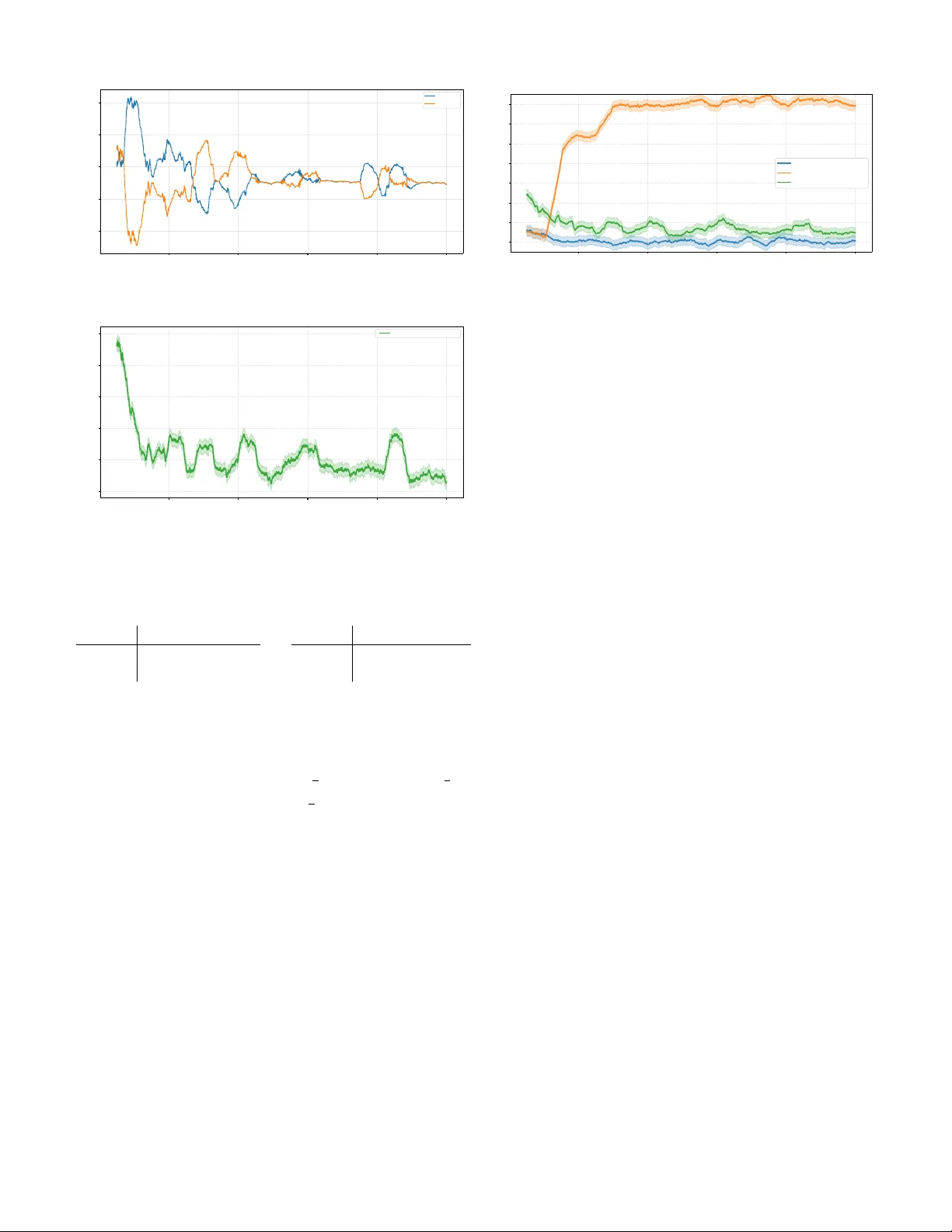
Decentralized MARL for Coarse Correlated Equilibrium in Aggre gati v e Marko v Games 1 st Siying Huang The School of Mathematical Sciences University of Chinese Academy of Sciences Beijing, China huangsiying@amss.ac.cn 2 nd Y ifen Mu SKLMS AMSS, CAS Beijing, China mu@amss.ac.cn 3 rd Ge Chen SKLMS AMSS, CAS Beijing, China chenge@amss.ac.cn Abstract —This paper studies the problem of decentralized learning of Coarse Correlated Equilibrium (CCE) in aggregativ e Markov games (AMGs), wher e each agent’s instantaneous reward depends only on its own action and an aggr egate quantity . Existing CCE learning algorithms for general Markov games are not designed to leverage the aggregativ e structure, and resear ch on decentralized CCE learning for AMGs remains limited. W e propose an adaptive stage-based V -learning algorithm that exploits the aggregative structure under a fully decentralized information setting . Based on the two-timescale idea, the algorithm partitions learning into stages and adjusts stage lengths based on the variability of aggregate signals, while using no-regr et updates within each stage. W e prov e the algorithm achieves an ϵ - approximate CCE in e O ( S A max T 5 /ϵ 2 ) episodes, avoiding the curse of multiagents which commonly arises in MARL. Numerical results verify the theoretical findings, and the decentralized, model-free design enables easy extension to large-scale multi-agent scenarios. Index T erms —aggr egative Markov games, coarse correlated equilibrium, decentralized learning, MARL, sample complexity I . I N T R O D U C T I O N Many sequential decision-making problems in the real world inv olve strategic interactions among multiple agents in a shared en vironment. Multi-agent reinforcement learning (MARL) provides an effecti ve framew ork for solving such problems, and has achiev ed success in many fields, including the game of Go [ 1 ], Poker [ 2 ], autonomous driving [ 3 ], and Large Language Models [ 4 ]. Howe ver , in practical systems, agents often make decisions based only on local observ ations, and centralized coordination is often impractical due to high communication costs or unreliable communication [ 5 ], [ 6 ]. Therefore, designing decentralized, communication-free, and scalable multi-agent learning algorithms is of great practical significance. Markov games [ 7 ] are a common mathematical framework for describing MARL. Under this framew ork, the core goal of multi-agent learning is usually to find a certain game equilibrium solution, such as Nash Equilibrium (NE) [ 8 ] and its variants. Howe ver , in general-sum scenarios, computing NE is PP AD-hard [ 9 ], [ 10 ], which makes learning NE face great challenges both in theory and practice. This research is supported by the National Key Research and Dev elopment Program of China (2022YF A1004600), the Natural Science Foundation of China (T2293770, 12288201). A natural alternative is the coarse correlated equilibrium (CCE) [ 11 ]. Unlik e NE, CCE in general-sum games can be computed in polynomial time [ 12 ]. More importantly , in normal-form games, CCE can be approximated when agents independently run no-regret learning algorithms [ 13 ]. This makes CCE well suited for decentralized learning. Accordingly , recent work has focused on learning CCE in Markov games and established sev eral sample complexity guarantees [ 14 ]–[ 16 ]. Despite these advances, most existing work treats the en vironment as fully general and does not exploit underlying structure [ 17 ], [ 18 ]. In fact, in practical scenarios such as market competition [ 19 ] and public resource allocation [ 20 ], an agent’ s reward usually depends only on its own behavior and an aggregate quantity . Such problems with an aggregati ve rew ard structure can be modeled as aggregati ve Marko v games (AMGs). This aggregati ve structure widely appears in demand response in power systems [ 21 ], resource allocation in communication networks [ 22 ], and pricing mechanisms based on aggregate demand in economic systems [ 23 ], making AMGs a class of game models with important application relev ance. Howe ver , existing work on AMGs is extremely limited. The few related studies mainly focus on network scenarios and continuous state spaces, and fail to consider decentralized CCE learning in AMGs. This leads to a natural question: Can we design decentralized algorithms that exploit the aggregati ve structure to efficiently learn CCE? T o address this question, this paper studies decentralized CCE learning in aggregati ve Markov games, and the main results are as follows: • W e propose an adaptiv e stage-based V -learning algorithm. The algorithm follows a two-timescale idea. It partitions each episode into stages to create a stable learning en vironment, and adaptively adjusts stage lengths based on the variability of the aggregate signal. W ithin each stage, Tsallis-INF no-regret learning is used to quickly update the policy to achiev e per-state no-regret. The algorithm is fully decentralized, and each agent makes decisions using only local information without communication. • W e show that if all agents independently run the proposed algorithm, an ϵ -approximate CCE can be found in at most e O ( S A max T 5 /ϵ 2 ) episodes, where S is the number of states, A max is the maximum action space size, and T is the episode length. This upper bound av oids dependence on the number of agents and matches existing sample complexity bounds of general Markov games [ 17 ], [ 18 ]. • W e provide numerical results to support the theoretical findings. Since the algorithm is decentralized and model- free, it can be easily scaled to large multi-agent systems. Paper Organization: Section II introduces preliminary definitions and notations; Section III details the proposed decentralized adaptive stage-based learning algorithm and core theoretical results; Section IV presents numerical simulations and analysis; Section V concludes the paper . I I . P R E L I M I NA R I E S Marko v game. An N -player episodic Markov game is defined by a tuple: {T , N , {S t } T t =1 , {A t i ( · ) } i ∈N ,t ∈T , { r t i } i ∈N ,t ∈T , { p t } t ∈T } , (1) where i) T = { 1 , 2 , . . . , T } is the set of finite time steps in each episode; ii) N = { 1 , 2 , . . . , N } is the set of agents; iii) S t is the finite state space at time t , where s t ∈ S t denotes the state of the system at time t , and {S t } T t =1 denote the collection of stage-wise state spaces; iv) A t i ( s t ) denotes the finite action space av ailable to agent i at time t when the system is in state s t ∈ S t , where a t i ∈ A t i ( s t ) is the action taken by agent i . The joint action space at time t is giv en by A t ( s t ) := Q i ∈N A t i ( s t ) , and a t = ( a t 1 , . . . , a t N ) ∈ A t ( s t ) denotes the action profile at time t ; v) r t i ( s t , a t ) ∈ [0 , 1] is the stage payoff (reward) of agent i at time t ; and vi) p t ( · | s t , a t ) ∈ ∆( S t +1 ) is the state transition kernel at time t , where ∆( S t +1 ) denotes the probability simplex over S t +1 . Notably , this formulation ( 1 ) allo ws time-varying state spaces S t and stage-dependent action spaces A t i ( s t ) , which captures finite-horizon problems with ev olving constraints. For notational con venience, we define S := max t ∈T |S t | , A i := max t ∈T max s t ∈S t |A t i ( s t ) | , ∀ i ∈ N , and A max := max i ∈N A i . Aggregati ve Markov game. W e consider a specialized class of Marko v games with aggregativ e stage-wise re ward structure, named aggr e gative Markov games (AMGs). Formally , the stage payof f (reward) of each agent i depends only on its local action and an aggregate of other agents’ actions: r t i ( s t , a t ) = r t i  s t , a t i , σ ( a t − i )  , ∀ i ∈ N , t ∈ T , where a t − i = ( a t j ) j  = i denotes the action profile of all agents except i , and function σ ( · ) is an aggregator (e.g., sum, average). Such structures arise in many large-scale systems where interactions are mediated through aggregate quantities, includ- ing congestion control, resource allocation in communication networks, and economic markets, where payoffs depend on summary statistics such as total demand or av erage load. This makes AMGs practically important and widely applicable, yet research on their decentralized learning remains scarce. Policy and value function. A (Markov) policy π i ( · ) := ( π 1 i ( · ) , . . . , π T i ( · )) for agent i is a sequence of step- t decision rules such that π t i ( s t ) ∈ ∆( A t i ( s t )) for all t ∈ T and s t ∈ S t , where π t i ( · ) maps the step- t state s t to a probability distribution ov er agent i ’ s feasible action space A t i ( s t ) at state s t . Let Π i denote the set of all Marko v policies for agent i , and Π = × N i =1 Π i denote the joint Markov policy space. Each agent aims to find a policy that maximizes its cumulati ve stage payoff over the T stages. A joint policy (or policy profile) π = ( π 1 , . . . , π N ) ∈ Π induces a probability measure over the sequence of states and joint actions. For a policy profile π , and for any t ∈ T , s ∈ S t , and a ∈ A t ( s t ) , the value function and the state-action value function (or Q -function) for agent i are defined as: V π t,i ( s ) := E π  T X t ′ = t r t ′ i ( s t ′ , a t ′ ) | s t = s  , (2) Q π t,i ( s, a ) := E π  T X t ′ = t r t ′ i ( s t ′ , a t ′ ) | s t = s, a t = a  . Best response and Nash equilibrium. For agent i , a pol- icy π ⋆ i is a best r esponse to π − i for a given initial state s 1 if V π ⋆ i , π − i 1 ,i ( s 1 ) = sup π i V π i , π − i 1 ,i ( s 1 ) . A policy profile π = ( π i , π − i ) ∈ Π is a Nash equilibrium (NE) if π i is a best response to π − i for all i ∈ N . Correlated policy . More generally , we define a (non-Marko v) corr elated policy as π = ( π 1 ( · ) , . . . , π T ( · )) , where for each time step t ∈ T , the step- t decision rule π t satisfies: π t ( z , s 1 , a 1 , . . . , s t − 1 , a t − 1 , s t ) ∈ ∆ ( A t ( s t )) for all s t ′ ∈ S t ′ , a t ′ ∈ A t ′ ( s t ′ ) (for t ′ ∈ { 1 , . . . , t − 1 } ), s t ∈ S t , and z ∈ R . The decision rule π t maps a random variable z ∈ R and a history of length t − 1 represented by ( s 1 , a 1 , . . . , s t − 1 , a t − 1 ) to a distribution over the joint action space. W e assume that the agents following a correlated policy can access a common source of randomness (e.g., a common random seed) for the random variable z . W e let π i = ( π 1 i ( · ) , . . . , π T i ( · )) and π − i = ( π 1 − i ( · ) , . . . , π T − i ( · )) be the proper marginal policies of π , whose step- t outputs are restricted to ∆( A t i ( s t )) and ∆( A t − i ( s t )) , respectiv ely . For non-Markov correlated policies, the v alue function at t = 1 is defined analogously to ( 2 ) . A best response π ⋆ i with respect to the non-Markov policies π − i is a policy (independent of the randomness of π − i ) that maximizes agent i ’ s value at step 1, i.e., V π ⋆ i , π − i 1 ,i ( s 1 ) = sup π i V π i , π − i 1 ,i ( s 1 ) , and is not necessarily Markov . Coarse correlated equilibrium. Giv en the PP AD-hardness of calculating NE in general-sum games [ 9 ], a widely used relaxation is coarse corr elated equilibrium (CCE). A CCE ensures no agent has the incentiv e to deviate from a correlated policy π by playing a different independent policy . Definition 2.1: (CCE). A correlated policy π is an ϵ - approximate coarse correlated equilibrium for any initial state s 1 ∈ S 1 if V π ⋆ i , π − i 1 ,i ( s 1 ) − V π 1 ,i ( s 1 ) ≤ ϵ, ∀ i ∈ N . CCE relaxes NE by allowing possible correlations in the policies, and NE is a special CCE in general-sum games [ 24 ]. Algorithm 1 Adaptive Stage-Based V -Learning with Tsallis-INF for CCE (Agent i ) 1: Initialize: V t,i ( s ) ← T − t + 1 , ˆ V t,i ( s ) ← T − t + 1 , D t ( s ) ← ∅ , ˜ C t ( s ) ← 0 , ˜ r t i ( s ) ← 0 , ˜ v t i ( s ) ← 0 , ˜ L t ( s ) ← T , π t i ( a | s ) ← 1 / |A t i ( s ) | , ˆ Q t,i ( s, a ) ← 0 , ∀ t ∈ T , s ∈ S t , a ∈ A t i ( s ) . 2: for episode k ← 1 to K do 3: Receiv e initial state s 1 ; 4: for step t ← 1 to T do 5: ˜ c := ˜ C t ( s t ) ← ˜ C t ( s t ) + 1 ; 6: T ake action a t i ∼ π t i ( · | s t ) , observe reward r t i and next state s t +1 , and compute aggregate quantity d t ; 7: D t ( s t ) ← D t ( s t ) ∪ { d t } ; 8: ˜ r t i ( s t ) ← ˜ r t i ( s t ) + r t i , ˜ v t i ( s t ) ← ˜ v t i ( s t ) + V t +1 ,i ( s t +1 ) ; 9: η i ← 2 p 1 / ˜ c ; 10: ˆ Q t,i ( s t , a t i ) ← ˆ Q t,i ( s t , a t i ) + [ T − t +1 − ( r t i + V t +1 ,i ( s t +1 ))] /T π t i ( a t i | s t ) ; 11: π t i ( a | s t ) ← 4( η i ( ˆ Q t,i ( s t , a ) − x )) − 2 , ∀ a ∈ A t i ( s t ) , where normalization factor x satisfies P a ∈A t i ( s t ) 4( η i ( ˆ Q t,i ( s t , a ) − x )) − 2 = 1 ; 12: if ˜ C t ( s t ) = ˜ L t ( s t ) then 13: // Entering a new stage 14: ˆ V t,i ( s t ) ← ˜ r t i ( s t ) ˜ c + ˜ v t i ( s t ) ˜ c + b ˜ c , where b ˜ c ← 4 p T 2 A i ι/ ˜ c ; 15: V t,i ( s t ) ← min { ˆ V t,i ( s t ) , T − t + 1 } ; 16: λ ( s t ) ← f ( D t ( s t )) //Adaptive fluctuation coefficient (Alg. 2 / 3 ) ; 17: ˜ L t ( s t ) ← ⌊ λ ( s t )(1 + 1 T ) ˜ L t ( s t ) ⌋ ; 18: D t ( s t ) ← ∅ , ˜ C t ( s t ) ← 0 , ˜ r t i ( s t ) ← 0 , ˜ v t i ( s t ) ← 0 ; 19: π t i ( a | s t ) ← 1 / |A t i ( s t ) | ; ˆ Q t,i ( s t , a ) ← 0 , ∀ a ∈ A t i ( s t ) ; 20: end if 21: end for 22: end for Decentralized learning . Agents interact in an unknown en vironment for K episodes, with the initial state s 1 drawn from a fixed distribution ρ ∈ ∆( S 1 ) . At each step t ∈ T , the agents observe the state s t ∈ S t , and take actions a t i ∈ A t i ( s t ) , i ∈ N simultaneously . Agent i then receives its priv ate stage payoff r t i ( s t , a t ) , and the environment transitions to the next state s t +1 ∼ p t ( ·| s t , a t ) . Notably , non-deterministic state transitions raise the difficulty of decentralized coordination, as agents cannot rely on fixed state trajectories for implicit alignment. W e focus on a fully decentralized setting: each agent only observes the states and its o wn rewards and actions, but not the re wards or actions of the other agents. In fact, in our algorithm, each agent is completely oblivious to the existence of the others, and does not communicate with each other . This decentralized information structure requires decision-making based solely on local information, and naturally arises in practical multi-agent systems where communication is limited or costly . I I I . D E C E N T R A L I Z E D C C E L E A R N I N G I N A M G S This section presents our decentralized learning algorithm for CCE in general-sum AMGs and establishes its sample complexity guarantees. A. Algorithmic Design Ideas In decentralized Marko v games, from the perspectiv e of any individual agent, the environment reduces to a single-agent Marko v decision process (MDP) within a single episode. Across multiple episodes, howe ver , the en vironment perceived by each agent becomes non-stationary , making it highly challenging for agents to simultaneously estimate v alue functions and optimize policies. A natural way to address this non-stationarity is a two- timescale design, a validated approach in decentralized multi- agent learning [ 25 ], [ 26 ]: value estimation is updated on a slo wer timescale to maintain a relativ ely stable learning target, while policy updates run on a faster timescale within stable phases. T o implement this idea, we partition the learning process into stag es with slo wly evolving value functions, inspired by stage-based V -learning [ 18 ]. W ithin each stage, we optimize policies via Tsallis-INF to achiev e per-s tate no-r e gr et learning. This combination of staged v alue stabilization and no-regret policy updates forms the core of our decentralized CCE learning framew ork. B. Algorithm Description Compared to general Markov games, the aggr egative payoff structure reduces ef fectiv e interaction complexity and provides additional information through observ able aggregate quantities that summarize collectiv e behavior . Our algorithm le verages this structure via an adaptiv e stage- based mechanism, as illustrated in Figure 1 . Agents first compute aggregate signals within each stage, then estimate a fluctuation coefficient to assess environmental stability , and finally adapt stage lengths based on this stability signal. This design allows the algorithm to adjust to varying levels of non- stationarity , distinguishing it from existing fixed-stage methods. Within Stage  End of Stage （ Line 6 - 7 ） Computes and Collect the Aggregate Signal   󰇛  󰇜 Estimate Fluctuation Coefficient 󰇛  󰇜 Based on   󰇛  󰇜 （ Line 16 ） Environment Stability Adapt Stage Length   󰇛  󰇜 Using 󰇛  󰇜 （ Line 17 ） Next Stage  +1 ◉ ◉ ◉ ◉ Episode   ⋮ Episode   Episode               Episode   Episode   ◉ ◉ Episode   ⋮ Fig. 1. Illustration of the adaptive stage-based mechanism. The adaptive stage-based V -learning algorithm for CCE is presented in Algorithm 1 , which is ex ecuted independently by each agent i ∈ N . The agent maintains upper confidence bounds on the value functions to activ ely explore the unkno wn en vironment, and updates value estimates independently via the aforementioned adaptiv e stage-based rule. For each step-state pair ( t, s t ) , the agent partitions its visitations into a sequence of stages . Each stage has a length ˜ L t ( s t ) , initialized as ˜ L t ( s t ) = T and updated at the end of each stage. The stage length is adjusted via a fluctuation coefficient λ ( s t ) computed from the sequence of observed aggregate quantities within the current stage, denoted by D t ( s t ) = { d t, 1 , . . . , d t,n } . Specifically , the next stage length is updated as ˜ L t ( s t ) ← ⌊ λ ( s t )(1 + 1 T ) ˜ L t ( s t ) ⌋ , so that stage lengths adapt to the observed aggregate volatility of the en vironment while growing at a near-geometric rate (1 + 1 /T ) [ 27 ]. In practice, λ ( s t ) can be computed using various stability metrics. W e adopt two common approaches: Coefficient of V ariation (CV) [ 28 ] (see Algorithm 2 ) or Mean Absolute Deviation (MAD) [ 29 ] (see Algorithm 3 ). When the visitation count ˜ C t ( s t ) reaches ˜ L t ( s t ) , the cur- rent stage ends and the agent updates its optimistic value estimate V t,i ( s t ) using only samples collected within this stage (Lines 12 – 19 ). All stage-specific statistics are then reset, and the policy is reinitialized to a uniform distrib ution for the next stage. This staged update helps maintain a relatively stable learning environment, mitigate multi-agent non-stationarity , and its near-geometric stage length growth aligns with the update logic of optimistic Q-learning with learning rate α t = T +1 T + t [ 30 ], [ 31 ]. At each time step t and state s t , agent i selects its action a t i by following a distribution π t i ( · | s t ) , which is updated via the Tsallis-INF adversarial bandit subroutine [ 32 ] (Lines 10 – 11 ) to guarantee per-state no-regret learning. The normalization Algorithm 2 Adaptiv e Fluctuation Coefficient f CV ( D t ( s t )) via CV 1: Input: Positiv e aggregate quantity sequence D t ( s t ) = { d t, 1 , . . . , d t,n } , minimum fluctuation coef ficient λ min ∈ ( T T +1 , 1] , empirical upper bound C V max 2: Output: Adaptiv e fluctuation coefficient λ ( s t ) ∈ [ λ min , 1] 3: if |D t ( s t ) | < 2 then 4: λ ( s t ) ← 1 ; // Default: no fluctuation (max stage length) 5: retur n λ ( s t ) 6: end if 7: ¯ d ← 1 |D t ( s t ) | P d t,j ∈D t ( s t ) d t,j ; 8: σ ← q 1 |D t ( s t ) |− 1 P d t,j ∈D t ( s t ) ( d t,j − ¯ d ) 2 ; 9: C V ← σ ¯ d ; 10: γ ← min  C V C V max , 1  ; 11: λ ( s t ) ← λ min + (1 − λ min ) · γ ; 12: retur n λ ( s t ) Algorithm 3 Adaptiv e Fluctuation Coefficient f MAD ( D t ( s t )) via MAD 1: Input: Positiv e aggregate quantity sequence D t ( s t ) = { d t, 1 , . . . , d t,n } , minimum fluctuation coef ficient λ min ∈ ( T T +1 , 1] , empirical upper bound M AD max 2: Output: Adaptiv e fluctuation coefficient λ ( s t ) ∈ [ λ min , 1] 3: if |D t ( s t ) | < 2 then 4: λ ( s t ) ← 1 ; // Default: no fluctuation 5: retur n λ ( s t ) 6: end if 7: ¯ d ← 1 |D t ( s t ) | P d t,j ∈D t ( s t ) d t,j ; 8: M AD ← 1 |D t ( s t ) | P d t,j ∈D t ( s t ) | d t,j − ¯ d | ; 9: γ ← min  M AD M AD max , 1  ; 10: λ ( s t ) ← λ min + (1 − λ min ) · γ ; 11: retur n λ ( s t ) factor in the policy update can be computed efficiently using Ne wton’ s method, with detailed steps provided in Algorithm 4 . T o obtain the final ϵ -approximate CCE policy , we construct a unified output policy ¯ π follo wing the certified policy frame work [ 33 ], as detailed in Algorithm 5 . Let π t,k i ( · | s t ) denote the policy of agent i at step t of episode k under state s t generated by Algorithm 1 . Agents use a shared random seed to uniformly sample an episode index from the previous stage, yielding the final correlated policy . This mild common randomness serves as a standard correlation device, which is only used for post- learning policy synchronization and does not break the fully decentralized learning paradigm. C. Theor etical Guarantees The following theorem presents the sample complexity guarantee of Algorithm 1 for learning CCE in general- sum aggregativ e Markov games. Our bound matches those established for general-sum Markov games in prior work [ 17 ], [ 18 ], [ 34 ]. Algorithm 4 Newton’ s Method approximation of π t i ( a | s t ) in Tsallis-Inf (Line 11 in Algorithm 1 ) 1: Input: s t , x, ˆ Q t,i ( · ) , η i //we use x from the last iteration as a warmstart 2: repeat 3: ∀ a ∈ A t i ( s t ) : π t i ( a | s t ) ← 4( η i ( ˆ Q t,i ( s t , a ) − x )) − 2 ; 4: x ← x − ( P a ∈A t i ( s t ) ˆ Q t,i ( s t ,a ) − 1) ( η i P a ∈A t i ( s t ) ˆ Q t,i ( s t ,a ) 3 2 ) ; 5: until con ver gence Algorithm 5 Construction of the Output Policy ¯ π 1: Input: The distribution trajectory specified by Algorithm 1 : { π t,k i : i ∈ N , t ∈ T , k ∈ [ K ] } ; 2: Uniformly sample k from [ K ] ; 3: for step t ← 1 to T do 4: Receiv e s t ; 5: Uniformly sample j from { 1 , 2 , . . . , ˜ c t,k ( s t ) } ; {For a state s t , ˜ c t,k denotes the number of visits to the state s t (at the t -th step) in the stage right before the current stage} 6: Set k ← ˜ l t,k j ; { ˜ l t,k j is the index of the episode that this state was visited the j -th time among the total ˜ c t,k times} 7: T ake joint action a t ∼ × N i =1 π t,k i ( · | s t ) ; 8: end for Theor em 3.1: (Sample complexity of learning CCE). For any p ∈ (0 , 1] , set ι = log(2 N S A max K T /p ) , and let the agents run Algorithm 1 for K episodes with K = O ( S A max T 5 ι/ϵ 2 ) . Then, with probability at least 1 − p , the output policy ¯ π of Algorithm 5 is an ϵ -approximate CCE. Pr oof sketch: W e provide a high-le vel overvie w of the proof and defer all technical details to Appendix A . The analysis proceeds in four main steps. Step 1 (Estimation and re gr et contr ol). W e first establish a high-probability bound on the stage-wise value estimation error . By combining martingale concentration arguments with the no- regret guarantee of the Tsallis-INF algorithm, we sho w that the empirical value estimates concentrate around their expectations up to an error of order O ( p T 2 A i ι/ ˜ c ) , which justifies the choice of the exploration bonus used in the algorithm (Line 14 ). Step 2 (Confidence bounds). W e construct optimistic upper v alue estimates V and pessimistic lower value estimates V , and prov e that they form valid high-probability confidence bounds. In particular , with high probability , V ⋆, ¯ π t,k − i t,i ( s t ) ≤ V k t,i ( s t ) , V ¯ π t,k t,i ( s t ) ≥ V k t,i ( s t ) , reducing the problem of bounding the CCE equilibrium gap to bounding the difference between these two estimates, V − V . Step 3 (Recursive err or pr opagation). Define δ t,k := V k t,i ( s t,k ) − V k t,i ( s t,k ) . W e sho w that δ t,k satisfies a recursiv e inequality: δ t,k ≤ I [ c t,k = 0] T + 1 ˜ c ˜ c X j =1 δ t +1 , ˜ l j + O ( b ˜ c ) . Unrolling this recursion and summing ov er episodes yields K X k =1 δ 1 ,k ≤ O  S T 3 + p S A max K T 5 ι  . Step 4 (Conclusion). A veraging ov er episodes and using the definition of the output policy ¯ π , we obtain V ⋆, ¯ π − i 1 ,i ( s 1 ) − V ¯ π 1 ,i ( s 1 ) ≤ O  p S A max T 5 ι/K  , which establishes the claimed sample complexity result. K e y Lemmas: The proof relies on the follo wing intermediate results, whose detailed proofs are provided in Appendix A . Lemma 3.2 (Estimation and r e gret bound): W ith probability at least 1 − p 2 , it holds for all agents i ∈ N , episodes k ∈ [ K ] , steps t ∈ T , and states s t ∈ S t that max π t i 1 ˜ c ˜ c X j =1 D π t i × π t, ˜ l j − i  r t i + P t V ˜ l j t +1 ,i  ( s t ) − 1 ˜ c ˜ c X j =1  r t i ( s t , a t, ˜ l j ) + V ˜ l j t +1 ,i ( s t +1 , ˜ l j )  ≤ 4 p T 2 A i ι/ ˜ c, where ι = log (4 N S A max K T /p ) . Lemma 3.3 (Confidence bounds): It holds with probability at least 1 − p that for all for all agents i ∈ N , episodes k ∈ [ K ] , steps t ∈ T , and states s t ∈ S t , V ⋆, ¯ π t,k − i t,i ( s t ) ≤ V k t,i ( s t ) , V ¯ π t,k t,i ( s t ) ≥ V k t,i ( s t ) . I V . S I M U L AT I O N S W e empirically ev aluate Algorithm 1 on the classic Fisher- men Game. The Fishermen Game is a simple 2 -horizon, 2 -agent Markov game adapted from [ 35 ]. It has two states S t = { s h , s ℓ } for t = 1 , 2 , where s h and s ℓ denote high and low fish stock lev els, respectiv ely . Each fisherman has a binary action set A t i = { a m , a f } for i = 1 , 2 and t = 1 , 2 , where a m = 5 represents intensi ve fishing with many nets, and a f = 3 means mild fishing with few nets. W e define the aggr e gate action as the total fishing effort across both agents, giv en by a = a 1 + a 2 where a i ∈ A t i . The re ward function for agent i in state s is formulated as an aggregati ve payoff (preserving the original game’ s reward values and structure): r i ( s, a ) = r i ( s, a 1 , a 2 ) = r i ( s, a i , a ) = f ( a i ) − g ( a ) − c ( s ) where the concav e priv ate payoff function is f ( a i ) = − 1 2 a 2 i + 23 2 a i + 1 , the conv ex aggregate cost function is g ( a ) = 1 4 a 2 − 1 2 a + 16 , and the state-dependent cost is c ( s h ) = 0 (no extra cost in high stock state), c ( s ℓ ) = 1 (extra cost in low stock 2000 4000 6000 8000 10000 Episode (Iterations) 18.5 19.0 19.5 20.0 20.5 Cumulative Reward Individual Cumulative Rewar d of T wo Agents Agent 1 Agent 2 Fig. 2. Individual cumulativ e rew ard of two agents. 2000 4000 6000 8000 10000 Episode (Iterations) 19.2 19.3 19.4 19.5 19.6 19.7 Average R eward Adaptive Stage-based Fig. 3. A verage rew ard of two agents. state). The resulting payoff matrices (rows: agent 1, columns: agent 2) are: s h a m (5) a f (3) a m (5) (10 , 10) (18 , 3) a f (3) (3 , 18) (9 , 9) s ℓ a m (5) a f (3) a m (5) (9 , 9) (17 , 2) a f (3) (2 , 17) (8 , 8) State transitions depend only on the current state s and all players’ actions a or the aggregate action a .Let P ( s ′ | s, a ) denote the transition probability to state s ′ from s giv en aggregate action a : P ( s h | s h , 6) = 1 , P ( s h | s h , 8) = 2 3 , P ( s h | s h , 10) = 1 5 , P ( s h | s ℓ , 6) = 1 , P ( s h | s ℓ , 8) = 1 2 , P ( s h | s ℓ , 10) = 0 , with P ( s ℓ | s, a ) = 1 − P ( s h | s, a ) . Consistent with the original design, a higher aggregate fishing effort a increases the likelihood of transitioning to the low fish stock state s ℓ . Figures 2 and 3 illustrate the indi vidual cumulativ e rewards of the two agents and the average re ward, respectively . The results show that the actual policy trajectories generated by our algorithm con ver ge to stable high rewards (around 19 . 2 – 19 . 5 per agent after sufficient episodes), which is a desirable empirical behavior beyond our theoretical guarantee (our theoretical results only guarantee con ver gence for the certified output policy). Moreover , Figure 2 clearly exhibits the stage-wise behavior of our algorithm: rew ards fluctuate noticeably at the beginning of each stage and then stabilize as learning proceeds within the stage. Finally , we compare our algorithm with two representative baselines in Figure 4 : centralized Q-learning (an ideal upper 2000 4000 6000 8000 10000 Episode (Iterations) 19.2 19.4 19.6 19.8 20.0 20.2 20.4 20.6 A verage Reward Fishermen Game: Convergence Comparison of Three Algorithms Independent Q Centralized Q Adaptive Stage-based Fig. 4. Rew ards comparison of three algorithms on the Fishing Game. “Centralized Q” denotes a centralized oracle that controls all agents’ actions to maximize the joint reward of both agents. “Independent Q” means each agent runs a naive single-agent Q-learning algorithm independently , taking greedy actions based only on local information without considering other agents. bound achiev ed by a fully coordinated oracle that can control the actions of both agents) and naiv e independent Q-learning (where each agent ignores other agents and the game structure). Empirical results show that our algorithm outperforms the independent baseline, demonstrating the effecti veness of our adaptiv e stage-based design in the decentralized setting. V . C O N C L U S I O N In this paper , we studied decentralized learning of Coarse Correlated Equilibrium (CCE) in aggregati ve Markov games (AMGs), a class of multi-agent systems where each agent’ s rew ard depends only on its own action and an aggregate of others’ actions. W e proposed an adapti ve stage-based V -learning algorithm that explicitly exploits the aggregati ve structure to enable efficient learning in a fully decentralized setting. W e established a sample complexity guarantee showing that the proposed method learns an ϵ -approximate CCE within e O ( S A max T 5 /ϵ 2 ) episodes, while notably avoiding the curse of multiagents. These results demonstrate that the aggregati ve structure can be harnessed to design efficient decentralized learning algorithms. Sev eral interesting directions remain for future research. First, it would be v aluable to further tighten the sample complexity bounds, potentially by refining the analysis or le veraging sharper concentration techniques. Second, extending the proposed framew ork to more general classes of structured Marko v games beyond the aggregati ve setting is a natural next step. Finally , it would be of interest to inv estigate whether similar ideas can be applied to learning other equilibrium concepts, such as correlated equilibrium or Nash equilibrium, in decentralized en vironments. R E F E R E N C E S [1] D. Silver, A. Huang, C. J. Maddison, A. Guez, L. Sifre, G. V an Den Driessche, J. Schrittwieser, I. Antonoglou, V . Panneershelvam, M. Lanctot et al. , “Mastering the game of Go with deep neural networks and tree search, ” Nature , vol. 529, no. 7587, pp. 484–489, 2016. [2] N. Brown and T . Sandholm, “Superhuman AI for heads-up no-limit poker: Libratus beats top professionals, ” Science , vol. 359, no. 6374, pp. 418–424, 2018. [3] B. R. Kiran, I. Sobh, V . T alpaert, P . Mannion, A. A. Al Sallab, S. Y ogamani, and P . Pérez, “Deep reinforcement learning for autonomous driving: A survey , ” IEEE transactions on intelligent transportation systems , vol. 23, no. 6, pp. 4909–4926, 2021. [4] G. Zhu, R. Zhou, W . Ji, and S. Zhao, “Lamarl: Llm-aided multi-agent reinforcement learning for cooperative policy generation, ” IEEE Robotics and Automation Letters , 2025. [5] S. Kar, J. M. F . Moura, and H. V . Poor, “ ⨿⌈ -learning: A collaborative distributed strategy for multi-agent reinforcement learning through consensus + innov ations, ” IEEE T ransactions on Signal Pr ocessing , vol. 61, no. 7, pp. 1848–1862, 2013. [6] V . J. Hodge, R. Hawkins, and R. Alexander, “Deep reinforcement learning for drone navigation using sensor data, ” Neural Computing and Applications , vol. 33, no. 6, pp. 2015–2033, 2021. [7] L. S. Shapley , “Stochastic games, ” Pr oceedings of the National Academy of Sciences , vol. 39, no. 10, pp. 1095–1100, 1953. [8] J. F . Nash Jr , “Equilibrium points in n-person games, ” Proceedings of the national academy of sciences , vol. 36, no. 1, pp. 48–49, 1950. [9] C. Daskalakis, P . W . Goldberg, and C. H. Papadimitriou, “The complexity of computing a Nash equilibrium, ” SIAM Journal on Computing , vol. 39, no. 1, pp. 195–259, 2009. [10] X. Chen, X. Deng, and S.-H. T eng, “Settling the complexity of computing two-player nash equilibria, ” Journal of the ACM (J ACM) , vol. 56, no. 3, pp. 1–57, 2009. [11] R. J. Aumann, “Correlated equilibrium as an expression of bayesian rationality , ” Econometrica: Journal of the Econometric Society , pp. 1–18, 1987. [12] C. H. Papadimitriou and T . Roughgarden, “Computing correlated equilibria in multi-player games, ” Journal of the ACM (J ACM) , vol. 55, no. 3, pp. 1–29, 2008. [13] S. Hart and A. Mas-Colell, “ A simple adaptiv e procedure leading to correlated equilibrium, ” Econometrica , vol. 68, no. 5, pp. 1127–1150, 2000. [14] Q. Liu, T . Y u, Y . Bai, and C. Jin, “ A sharp analysis of model-based reinforcement learning with self-play , ” in International Confer ence on Machine Learning , 2021. [15] W . Mao and T . Ba ¸ sar , “Provably efficient reinforcement learning in decentralized general-sum Markov games, ” Dynamic Games and Applications , pp. 1–22, 2022. [16] Y . Cai, H. Luo, C.-Y . W ei, and W . Zheng, “Near-optimal policy optimization for correlated equilibrium in general-sum markov games, ” in International Confer ence on Artificial Intelligence and Statistics . PMLR, 2024, pp. 3889–3897. [17] C. Jin, Q. Liu, Y . W ang, and T . Y u, “V -learning–A simple, efficient, decen- tralized algorithm for multiagent RL, ” arXiv pr eprint arXiv:2110.14555 , 2021. [18] W . Mao, L. Y ang, K. Zhang, and T . Basar , “On improving model- free algorithms for decentralized multi-agent reinforcement learning, ” in International Confer ence on Machine Learning . PMLR, 2022, pp. 15 007–15 049. [19] K. Iyer, R. Johari, and C. C. Moallemi, “Information aggregation and allocativ e efficiency in smooth markets, ” Management Science , vol. 60, no. 10, pp. 2509–2524, 2014. [20] E. S. Mills, “ An aggregati ve model of resource allocation in a metropolitan area, ” The American Economic Review , vol. 57, no. 2, pp. 197–210, 1967. [21] M. Y e and G. Hu, “Game design and analysis for price-based demand re- sponse: An aggregate game approach, ” IEEE transactions on cybernetics , vol. 47, no. 3, pp. 720–730, 2016. [22] H.-S. Liao, P .-Y . Chen, and W .-T . Chen, “ An efficient downlink radio resource allocation with carrier aggregation in lte-advanced networks, ” IEEE T ransactions on Mobile Computing , vol. 13, no. 10, pp. 2229–2239, 2014. [23] V . Nocke and N. Schutz, “Multiproduct-firm oligopoly: An aggregativ e games approach, ” Econometrica , vol. 86, no. 2, pp. 523–557, 2018. [24] N. Nisan, T . Roughgarden, E. T ardos, and V . V . V azirani, Algorithmic Game Theory . Cambridge University Press, 2007. [25] M. Sayin, K. Zhang, D. Leslie, T . Basar , and A. Ozdaglar, “Decentralized q-learning in zero-sum markov games, ” Advances in Neural Information Pr ocessing Systems , vol. 34, pp. 18 320–18 334, 2021. [26] M. O. Sayin, F . Parise, and A. Ozdaglar , “Fictitious play in zero-sum stochastic games, ” SIAM Journal on Control and Optimization , vol. 60, no. 4, pp. 2095–2114, 2022. [27] Z. Zhang, Y . Zhou, and X. Ji, “ Almost optimal model-free reinforcement learning via reference-advantage decomposition, ” Advances in Neural Information Processing Systems , vol. 33, 2020. [28] W . A. Hendricks and K. W . Robey , “The sampling distribution of the coefficient of variation, ” The Annals of Mathematical Statistics , vol. 7, no. 3, pp. 129–132, 1936. [29] R. C. Geary , “The ratio of the mean deviation to the standard deviation as a test of normality , ” Biometrika , vol. 27, no. 3/4, pp. 310–332, 1935. [30] C. Jin, Z. Allen-Zhu, S. Bubeck, and M. I. Jordan, “Is Q-learning provably efficient?” in International Conference on Neural Information Processing Systems , 2018, pp. 4868–4878. [31] Y . Bai, T . Xie, N. Jiang, and Y .-X. W ang, “Provably efficient q-learning with low switching cost, ” Advances in Neural Information Pr ocessing Systems , vol. 32, 2019. [32] J. Zimmert and Y . Seldin, “Tsallis-inf: An optimal algorithm for stochastic and adversarial bandits, ” Journal of Machine Learning Resear ch , vol. 22, no. 28, pp. 1–49, 2021. [33] Y . Bai, C. Jin, and T . Y u, “Near-optimal reinforcement learning with self-play , ” Advances in Neural Information Processing Systems , vol. 33, 2020. [34] Z. Song, S. Mei, and Y . Bai, “When can we learn general-sum Markov games with a large number of players sample-efficiently?” arXiv pr eprint arXiv:2110.04184 , 2021. [35] M. Maschler, S. Zamir, and E. Solan, Game Theory . Cambridge Univ . Press, 2020. A P P E N D I X A P R O O F S F O R S E C T I O N I I I W e first introduce a few notations to facilitate the analysis. For a step t ∈ T of an episode k ∈ [ K ] , we denote by s t,k the state that the agents observe at this time step. For any state s t ∈ S t , we let π t,k i ( · | s t ) ∈ ∆( A t i ( s t )) be the distribution prescribed by Algorithm 1 to agent i at this step. Notice that such notations are well-defined for ev ery s t ∈ S t ev en if s t might not be the state s t,k that is actually visited at the giv en step. W e further let π t,k i = { π t,k i ( · | s t ) : s t ∈ S t } , and let a t,k i ∈ A t i ( s t ) be the actual action taken by agent i . For any s t ∈ S t , let ˜ C t,k ( s t ) denotes the value of ˜ C t ( s t ) at the be ginning of the k -th episode. Note that it is proper to use the same notation to denote these values from all the agents’ perspectiv es, because the agents maintain the same estimates of these terms as they can be calculated from the common observ ations (of the state-visitation). W e also use V k t,i ( s t ) and ˆ V k t,i ( s t ) to denote the values of V t,i ( s t ) and ˆ V t,i ( s t ) , respectiv ely , at the beginning of the k -th episode from agent i ’ s perspective. Further , for a state s t,k , let ˜ c t,k denote the number of times that state s t,k has been visited (at the t -th step) in the stage right before the current stage, and let ˜ l t,k j denote the index of the episode that this state was visited the j -th time among the ˜ c t,k times. For notational con v enience, we use ˜ c to denote ˜ c t,k , and ˜ l j to denote ˜ l t,k j , whene ver t and k are clear from the context. With the new notations, the update rule in Line 14 of Algorithm 1 can be equiv alently expressed as ˆ V t,i ( s t ) ← 1 ˜ c ˜ c X j =1  r t i ( s t , a t, ˜ l j ) + V ˜ l j t +1 ,i ( s t +1 , ˜ l j )  + b ˜ c . (3) T o streamline the Bellman equations for the value and Q- functions, we introduce two auxiliary operators. First, for any stage- t state-action pair ( s t , a t ) and any value function V defined on the stage- t + 1 state space S t +1 , the state transition operator is P t V ( s t , a t ) := E s t +1 ∼ p t ( ·| s t , a t ) V  s t +1  . Second, for a joint polic y profile π = ( π t i ) i ∈N ,t ∈T , we define the stage- t marginal joint decision rule as π t := ( π t 1 , π t 2 , . . . , π t N ) , which is the collection of stage- t decision rules of all agents extracted from the full joint Marko v policy π . For any stage- t state s t and any Q-function Q defined on ( s t , A t ( s t )) , the policy expectation operator is D π t Q ( s t ) := E a t ∼ π t ( ·| s t ) Q ( s t , a t ) , where a t ∼ π t ( · | s t ) means the joint action a t is sampled from the product distribution induced by π t at state s t . W ith these notations and definitions, the Bellman equations for the joint value and Q-functions can be written succinctly as Q π t ( s t , a t ) =  r t + P t V π t +1  ( s t , a t ) , (4) V π t ( s t ) = ( D π t Q π t ) ( s t ) (5) for all t ∈ T , s t ∈ S t , and a t ∈ A t ( s t ) . In the following proof, we assume without loss of generality that the initial state s 1 is fixed (i.e., the initial state distribution ρ is a point mass at s 1 ). Our proof can be straightforwardly generalized to the case where s 1 is drawn from an arbitrary fixed distribution ρ ∈ ∆( S 1 ) . In the following, we start with an intermediate result, which justifies our choice of the bonus term. Lemma A.1: W ith probability at least 1 − p 2 , it holds for all agents i ∈ N , episodes k ∈ [ K ] , steps t ∈ T , and states s t ∈ S t that max π t i 1 ˜ c ˜ c X j =1 D π t i × π t, ˜ l j − i  r t i + P t V ˜ l j t +1 ,i  ( s t ) − 1 ˜ c ˜ c X j =1  r t i ( s t , a t, ˜ l j ) + V ˜ l j t +1 ,i ( s t +1 , ˜ l j )  ≤ 4 p T 2 A i ι/ ˜ c, where ι = log (4 N S A max K T /p ) . Pr oof: W e proceed the proof in three key steps. Step 1: Sample average error bound via martingale differences. For a fixed agent i ∈ N , episode k ∈ [ K ] , step t ∈ T , and state s t ∈ S t , let F j be the σ -algebra generated by all the random variables up to episode ˜ l j . Then,  r t i ( s t , a t, ˜ l j i ) + V ˜ l j t +1 ,i ( s t +1 , ˜ l j ) − D π t, ˜ l j  r t i + P t V ˜ l j t +1 ,i  ( s t )  ˜ c j =1 is a martingale difference sequence with respect to {F j } ˜ c j =1 . By the boundedness of rewards and value functions, this sequence is bounded by H . Applying the Azuma-Hoeffding inequality , with probability at least 1 − p/ (4 N S T K ) , we hav e 1 ˜ c ˜ c X j =1 D π t, ˜ l j  r t i + P t V ˜ l j t +1 ,i  ( s t ) − 1 ˜ c ˜ c X j =1  r t i ( s t , a t, ˜ l j ) + V ˜ l j t +1 ,i ( s t +1 , ˜ l j )  ≤ p 2 T 2 log(8 N S K T /p ) / ˜ c ≤ p 2 T 2 ι/ ˜ c ≤ p T 2 A i ι/ ˜ c. (6) Step 2: Regret bound via Tsallis-INF . Then, we only need to bound R ⋆ ˜ c := max π t i 1 ˜ c ˜ c X j =1 D π t i × π t, ˜ l j − i  r t i + P t V ˜ l j t +1 ,i  ( s t ) − 1 ˜ c ˜ c X j =1 D π t, ˜ l j  r t i + P t V ˜ l j t +1 ,i  ( s t ) . (7) Notice that R ⋆ ˜ c can be considered as the averaged regret of visiting the state s t with respect to the optimal policy in hindsight. Such a regret minimization problem can be handled by an adversarial multi-armed bandit problem, where the loss function at step j ∈ [ ˜ c ] is defined as ℓ j ( a t i ) = E a t − i ∼ π t, ˜ l j − i ( s t )  T − t + 1 − r t i ( s t , a t ) − P t V ˜ l j t +1 ,i ( s t , a t )  /T . Algorithm 1 adopts the Tsallis-INF algorithm [ 32 ], which guarantees for all k ∈ [ K ] : R ⋆ ˜ c = max a t i T ˜ c ˜ c X j =1 ( − ℓ j ( a i )) − T ˜ c ˜ c X j =1 E a t i ∼ π t, ˜ l j i ( s t )[ − ℓ j ( a t i )] = T ˜ c  ˜ c X j =1 E a t i ∼ π t, ˜ l j i ( s t )[ ℓ j ( a t i )] − min a t i ˜ c X j =1 ℓ j ( a t i )  ≤ T ˜ c (4 p A i ˜ c + 1) = 4 r T 2 A i ˜ c + T ˜ c ≤ 3 p T 2 A i ι/ ˜ c. (8) Step 3: Union bound. Combining ( 6 ) and ( 8 ) , and taking a union bound over all agents i ∈ N , episodes k ∈ [ K ] , steps t ∈ T , and states s t ∈ S t , completes the proof. ■ Based on the trajectory of the distributions { π t,k i : i ∈ N , t ∈ T , k ∈ [ K ] } specified by Algorithm 1 , we construct a correlated policy ¯ π t,k for each ( t, k ) ∈ T × [ K ] . Our construction of the correlated policies, largely inspired by the “certified policies” [ 33 ] for learning in two-player zero-sum games, is formally presented in Algorithm 6 . W e further define an output policy ¯ π : first uniformly sample an index k from [ K ] , then ex ecute the policy ¯ π 1 ,k . A formal description of ¯ π is given in Algorithm 5 . By construction of the correlated policies ¯ π t,k , we know that for any i ∈ N , episode k ∈ [ K ] , Algorithm 6 Construction of the Correlated Policy ¯ π t,k 1: Input: The distribution trajectory { π t,k i : i ∈ N , t ∈ T , k ∈ [ K ] } specified by Algorithm 1 . 2: Initialize: k ′ ← k . 3: for step t ′ ← t to T do 4: Receiv e s t ′ ; 5: Uniformly sample j from { 1 , 2 , . . . , ˜ c t ′ ,k ′ ( s t ′ ) } ; 6: Set k ′ ← ˜ l t ′ ,k ′ j ; { ˜ l t ′ ,k ′ j is the index of the episode that this state was visited the j -th time (among the total ˜ c t ′ ,k ′ times) in the last stage} 7: T ake joint action a t ′ ∼ × N i =1 π t ′ ,k ′ i ( · | s t ′ ) ; 8: end for step t ∈ [ T + 1] , and state s t ∈ S t , the corresponding value function can be written recursiv ely as follows: V ¯ π t,k t,i ( s t ) = 1 ˜ c ˜ c X j =1 D π t, ˜ l j  r t i + P t V ¯ π t +1 , ˜ l j t +1 ,i  ( s t ) , and V ¯ π t,k t,i ( s t ) = 0 if t = T + 1 or k is in the first stage of the corresponding ( t, s t ) pair . W e also immediately obtain that V ¯ π 1 ,i ( s 1 ) = 1 K K X k =1 V ¯ π 1 ,k 1 ,i ( s 1 ) . For analytical purposes, we introduce two auxiliary notations V and ˆ V as lower confidence bounds of the value estimates. Specifically , for any i ∈ N , episode k ∈ [ K ] , step t ∈ [ T + 1] , and state s t ∈ S t , we define V k t,i ( s t ) = ˆ V k t,i ( s t ) = 0 if t = T + 1 or k is in the first stage of the ( h, s t ) pair , and ˆ V k t,i ( s t ) = 1 ˜ c ˜ c X j =1  r t i ( s t , a t, ˜ l j ) + V ˜ l j t +1 ,i ( s t +1 , ˜ l j )  − b ˜ c , and V k t,i ( s t ) = max n ˆ V k t,i ( s t ) , 0 o . Note that these notations are only for analysis and agents do not need to maintain them explicitly during learning. Further , recall that V ⋆, ¯ π t,k − i t,i ( s t ) is agent i ’ s best response value against its opponents’ polic y ¯ π t,k − i . Our next lemma shows that V k t,i ( s t ) and V k t,i ( s t ) are indeed valid upper and lower bounds of V ⋆, ¯ π t,k − i t,i ( s t ) and V ¯ π t,k t,i ( s t ) , respectiv ely . Lemma A.2: It holds with probability at least 1 − p that for all for all agents i ∈ N , episodes k ∈ [ K ] , steps t ∈ T , and states s t ∈ S t , V ⋆, ¯ π t,k − i t,i ( s t ) ≤ V k t,i ( s t ) , (9) V ¯ π t,k t,i ( s t ) ≥ V k t,i ( s t ) . (10) Pr oof: Fix an agent i ∈ N , episode k ∈ [ K ] , step t ∈ T , and state s t ∈ S t . The desired result clearly holds for any state s t that is in its first stage, due to our initialization of V k t,i ( s t ) and V k t,i ( s t ) for this special case. In the follo wing, we only need to focus on the case where V k t,i ( s t ) and V k t,i ( s t ) hav e been updated at least once at the giv en state s t before the k -th episode. W e first prove the first inequality ( 9 ) . It suffices to show that ˆ V k t,i ( s t ) ≥ V ⋆, ¯ π t,k − i t,i ( s t ) , since V k t,i ( s t ) = min { ˆ V k t,i ( s t ) , T − t + 1 } , and V ⋆, ¯ π t,k − i t,i ( s t ) is always less than or equal to T − t + 1 . Our proof relies on induction on k ∈ [ K ] . The base case k = 1 holds by initialization logic. For the inductiv e step, consider two cases for t ∈ T and s t ∈ S t : Case 1 (for ( 9 ) ): ˆ V t,i ( s t ) has just been updated in (the end of) episode k − 1 . In this case, by definition of stage-based updates: ˆ V k t,i ( s t ) = 1 ˜ c ˜ c X j =1  r t i ( s t , a t, ˜ l j ) + V ˜ l j t +1 ,i ( s t +1 , ˜ l j )  + b ˜ c . (11) And by the definition of V ⋆, ¯ π t,k − i t ( s t ) , it holds with probability at least 1 − p 4 N S K T that V ⋆, ¯ π t,k − i t,i ( s t ) ≤ max π t i 1 ˜ c ˜ c X j =1 D π t i × π t, ˜ l j − i r t i + P t V ⋆, ¯ π t +1 , ˜ l j − i t +1 ,i ! ( s t ) ≤ max π t i 1 ˜ c ˜ c X j =1 D π t i × π t, ˜ l j − i  r t i + P t V ˜ l j t +1 ,i  ( s t ) ≤ 1 ˜ c ˜ c X j =1  r t i ( s t , a t, ˜ l j ) + V ˜ l j t +1 ,i ( s t +1 , ˜ l j )  + 4 p T 2 A i ι/ ˜ c ≤ ˆ V k t,i ( s t ) , (12) where the second step is by the induction hypothesis, the third step holds due to Lemma A.1 , and the last step is by the definition of b ˜ c . Case 2 (for ( 9 ) ): ˆ V t,i ( s t ) was not updated in (the end of) episode k − 1 . Since we have excluded the case that ˆ V t,i has nev er been updated, we are guaranteed that there exists an episode j such that ˆ V t,i ( s t ) has been updated in the end of episode j − 1 most recently . In this case, ˆ V k t,i ( s t ) = ˆ V k − 1 t,i ( s t ) = · · · = ˆ V j t,i ( s t ) ≥ V ⋆, ¯ π t,j − i t,i ( s t ) , where the last step is by the induction hypothesis. Finally , by the construction of stage- based policies (Algorithm 1 ), ¯ π t,j − i is constant within the same stage (i.e., unchanged for episodes in that stage), so V ⋆, ¯ π t,j − i t,i ( s t ) is also constant for all episodes j in the same stage. Since we know that episode j and episode k lie in the same stage, we can conclude that V ⋆, ¯ π t,k − i t,i ( s t ) = V ⋆, ¯ π t,j − i t,i ( s t ) ≤ ˆ V k t,i ( s t ) . Combining the two cases and applying a union bound over all agents i ∈ N , episodes k ∈ [ K ] , steps t ∈ T , and states s t ∈ S t , the first inequality holds with probability at least 1 − p 2 . Next, we prove the second inequality ( 10 ) in the statement of the lemma. Notice that it suffices to show ˆ V k t,i ( s t ) ≤ V ¯ π t,k t,i ( s t ) because V k t,i ( s t ) = max { ˆ V k t,i ( s t ) , 0 } . Our proof again relies on induction on k ∈ [ K ] . Similar to the proof of the first inequality , the claim apparently holds for k = 1 , and we consider the following two cases for each step t ∈ T and s t ∈ S t . Case 1 (for ( 10 ) ): The value of ˆ V t,i ( s t ) has just changed in (the end of) episode k − 1 . In this case, ˆ V k t,i ( s t ) = 1 ˜ c ˜ c X j =1  r t i ( s t , a t, ˜ l j ) + ˆ V ˜ l j t +1 ,i ( s t +1 , ˜ l j )  − b ˜ c . (13) By the definition of V ¯ π t,k t,i ( s t ) , it holds with probability at least 1 − p 4 N S K T that V ¯ π t,k t,i ( s t ) = 1 ˜ c ˜ c X j =1 D π t, ˜ l j  r t i + P t V ¯ π t +1 , ˜ l j t +1 ,i  ( s t ) ≥ 1 ˜ c ˜ c X j =1 D π t, ˜ l j  r t i + P t ˆ V ˜ l j t +1 ,i  ( s t ) ≥ 1 ˜ c ˜ c X j =1  r t i ( s t , a t, ˜ l j ) + ˆ V ˜ l j t +1 ,i ( s t +1 , ˜ l j )  − p 2 T 2 ι/ ˜ c ≥ ˆ V k t,i ( s t ) , (14) where the second step is by the induction hypothesis, the third step holds due to the Azuma-Hoef fding inequality , and the last step is by the definition of b ˜ c . Case 2 (for ( 10 ) ): The value of ˆ V t,i ( s t ) has not changed in (the end of) episode k − 1 . Since we have excluded the case that ˆ V t,i has nev er been updated, we are guaranteed that there exists an episode j such that ˆ V t,i ( s t ) has changed in the end of episode j − 1 most recently . In this case, we know that indices j and k belong to the same stage, and ˆ V k t,i ( s t ) = ˆ V k − 1 t,i ( s t ) = · · · = ˆ V j t,i ( s t ) ≤ V ¯ π t,j t,i ( s t ) , where the last step is by the induction hypothesis. Finally , by stage- based policy construction (Algorithm 1 ), ¯ π t,j is constant within the same stage, so V ¯ π t,j t,i ( s t ) is constant for all episodes j in that stage. Since j and k lie in the same stage, we can conclude that V ¯ π t,k t,i ( s t ) = V ¯ π t,j t,i ( s t ) ≥ ˆ V k t,i ( s t ) . Again, combining the two cases and applying a union bound ov er all agents i ∈ N , episodes k ∈ [ K ] , steps t ∈ T , and states s t ∈ S t , the second inequality holds with probability at least 1 − p 2 . By the union bound ov er both inequalities, the lemma holds with probability at least 1 − p . ■ The follo wing result shows that the agents hav e no incentiv e to deviate from the correlated policy ¯ π , up to a regret term of the order e O ( p T 5 S A max /K ) . Theor em A.3: For an y p ∈ (0 , 1] , let ι = log(2 N S A max K T /p ) . Suppose K ≥ S T A max ι , with probability at least 1 − p , the following holds for any initial state s 1 ∈ S 1 and agent i ∈ N : V ⋆, ¯ π − i 1 ,i ( s 1 ) − V ¯ π 1 ,i ( s 1 ) ≤ O  p T 5 S A max ι/K  . Pr oof: W e first recall the definitions of several notations and define a few new ones. For a state s t,k , recall that ˜ c t,k denotes the number of visits to the state s t,k (at the t -th step) in the stage right before the current stage, and ˜ l t,k j denotes the j -th episode among the ˜ c t,k episodes. When t and k are clear from context, we abbreviate ˜ l t,k j as ˜ l j and ˜ c t,k as ˜ c . By Lemma A.2 (upper/lower bound properties of V and V ) and the construction of the output policy ¯ π in Algorithm 1 , we know that V ⋆, ¯ π − i 1 ,i ( s 1 ) − V ¯ π 1 ,i ( s 1 ) ≤ 1 K K X k =1  V ⋆, ¯ π k 1 , − i 1 ,i ( s 1 ) − V ¯ π k 1 1 ,i ( s 1 )  ≤ 1 K K X k =1  V k 1 ,i ( s 1 ) − V k 1 ,i ( s 1 )  . Thus, it suffices to upper bound 1 K P K k =1 ( V k 1 ,i ( s 1 ) − V k 1 ,i ( s 1 )) . For a fixed agent i ∈ N , we define the following notation: δ t,k := V k t,i ( s t,k ) − V k t,i ( s t,k ) . The key idea of the subsequent proof is to upper bound P K k =1 δ t,k by the next step P K k =1 δ t +1 ,k , and then obtain a recursiv e formula. From the update rule of V k t,i ( s t,k ) in ( 3 ) , we hav e: V k t,i ( s t,k ) ≤ I [ c t,k = 0] T + 1 ˜ c ˜ c X j =1  r t i ( s t , a t, ˜ l j ) + V ˜ l j t +1 ,i ( s t +1 , ˜ l j )  + b ˜ c , where the I [ c t,k = 0] term counts for the ev ent that the optimistic value function has nev er been updated for the giv en state. Combining this with the definition of V k t,i ( s t,k ) , we hav e δ t,k ≤ I [ c t,k = 0] T + 1 ˜ c ˜ c X j =1  V ˜ l j t +1 ,i ( s t +1 , ˜ l j ) − V ˜ l j t +1 ,i ( s t +1 , ˜ l j )  + 2 b ˜ c ≤ I [ c t,k = 0] T + 1 ˜ c ˜ c X j =1 δ t +1 , ˜ l j + 2 b ˜ c , (15) T o find an upper bound of P K k =1 δ t,k , we proceed to upper bound each term on the RHS of ( 15 ) separately: T erm 1: P K k =1 I [ c t,k = 0] T . Each fixed step-state pair ( t, s t ) contributes at most 1 to P K k =1 I  c t,k = 0  . There are S T such pairs (across t ∈ T and s t ∈ S t ), so P K k =1 I [ c t,k = 0] T ≤ S T 2 . T erm 2: P K k =1 1 ˜ c t,k P ˜ c t,k j =1 δ t +1 , ˜ l t,k j . Switching the order of summation, we rewrite this term as: K X k =1 1 ˜ c t,k ˜ c t,k X j =1 δ t +1 , ˜ l t,k j = K X k =1 K X m =1 1 ˜ c t,k δ t +1 ,m ˜ c t,k X j =1 I h ˜ l t,k j = m i = K X m =1 δ t +1 ,m K X k =1 1 ˜ c t,k ˜ c t,k X j =1 I h ˜ l t,k j = m i . (16) For a fixed episode m , notice that P ˜ c t,k j =1 I [ ˜ l t,k j = m ] ≤ 1 , and that P ˜ c t,k j =1 I [ ˜ l t,k j = m ] = 1 happens if and only if s t,k = s t,m and ( t, m ) lies in the previous stage of ( t, k ) with respect to the step-state pair ( t, s t,k ) . Define K m := { k ∈ [ K ] : P ˜ c t,k j =1 I [ ˜ l t,k j = m ] = 1 } ; this set consists of all episodes k for which m is a pre-stage episode of ( t, s t,k ) . Then we kno w that all episode indices k ∈ K m belong to the same stage, and hence these episodes hav e the same value of ˜ c t,k . That is, there exists an integer N m > 0 , such that ˜ c t,k = N m , ∀ k ∈ K m . Further , since the stages are partitioned in a way such that each stage is at most (1 + 1 T ) times longer than the previous stage (Line 17 of Algorithm 1 ), we know that |K m | ≤ (1 + 1 T ) N m . Therefore, for ev ery m , it holds that K X k =1 1 ˜ c t,k ˜ c t,k X j =1 I h ˜ l t,k j = m i ≤ 1 + 1 T . (17) Combining ( 16 ) and ( 17 ) leads to the following upper bound of the second term in ( 15 ): K X k =1 1 ˜ c t,k ˜ c t,k X j =1 δ t +1 , ˜ l k t,j ≤ (1 + 1 T ) K X k =1 δ t +1 ,k . (18) So far , we have obtained the following upper bound: K X k =1 δ t,k ≤ S T 2 + (1 + 1 T ) K X k =1 δ t +1 ,k + 2 K X k =1 b ˜ c t,k . Iterating the abov e inequality ov er t = T , T − 1 , . . . , 1 leads to K X k =1 δ 1 ,k ≤ T X t =1 (1 + 1 T ) t − 1 ! S T 2 + 2 T X t =1 K X k =1 (1 + 1 T ) t − 1 b ˜ c t,k =  (1 + 1 T ) T − 1  S T 3 + 2 T X t =1 K X k =1 (1 + 1 T ) t − 1 b ˜ c t,k ≤ O S T 3 + T X t =1 K X k =1 (1 + 1 T ) t − 1 b ˜ c t,k ! , (19) where we used the fact that (1 + 1 T ) T ≤ e . T erm 3: Analysis of b ˜ c t,k . In the follo wing, we analyze the bonus term b ˜ c t,k .Recall that for any state s t , when the number of visits ˜ C t,k to ( t, s t ) reaches the predefined stage length (i.e., ˜ C t ( s t ) = ˜ L t ( s t ) ), the algorithm enters a new stage. The adaptiv e stage length is updated as ˜ L t ( s t ) ← ⌊ λ ( s t )(1 + 1 T ) ˜ L t ( s t ) ⌋ , where λ ( s t ) ∈ ( T T +1 , 1] ; the bonus term is defined as b ˜ c = 4 p T 2 A i ι/ ˜ c . For con venience, we introduce auxiliary notations for adaptiv e stage lengths: let e s t , 1 = T and e s t ,j +1 = ⌊ λ ( s t )(1 + 1 T ) e s t ,j ⌋ for j ≥ 1 . For any t ∈ T , we decompose the sum ov er k by state s t and stage length e s t ,j : K X k =1 (1 + 1 T ) t − 1 b ˜ c t,k ≤ K X k =1 (1 + 1 T ) t − 1 4 q T 2 A i ι/ ˜ C t,k =4 p T 2 A i ι X s t ∈S t X j ≥ 1 (1 + 1 T ) t − 1 × e − 1 2 s t ,j K X k =1 I h s t,k = s t , ˜ C t,k ( s t,k ) = e s t ,j i =4 p T 2 A i ι X s t ∈S t X j ≥ 1 (1 + 1 T ) t − 1 w ( s t , j ) e − 1 2 s t ,j , where we define w ( s t , j ) := K X k =1 I { s t,k = s t , ˜ C t,k ( s t,k ) = e j } , for any s t ∈ S t (number of episodes where ( t, s t ) has pre- stage length e s t ,j ). If we further let w ( s t ) := P j ≥ 1 w ( s t , j ) , we can see that P s t ∈S t w ( s t ) = K . For each fixed state s t , we now seek an upper bound of its corresponding j value, denoted as J in what follows. By the stage update rule, for any 1 ≤ j ≤ J : ⌊ λ min (1 + 1 T ) e s t ,j ⌋ ≤ w ( s t , j ) = K X k =1 I h s t,k = s t , ˜ C t,k ( s t,k ) = e s t ,j i ≤ ⌊ (1 + 1 T ) e s t ,j ⌋ , where λ min ∈ ( T T +1 , 1] . Thus, the sequence { e s t ,j } grows almost geometrically with ratio ρ ∈ (1 , 1 + 1 T ] , which can also be written as ρ = 1 + c T for some constant c ∈ (0 , 1] . By the formula for the sum of a geometric sequence, it follows that J X j =1 e s t ,j = Θ  T c e s t , 1 [ ρ J − 1]  = Θ ( T e s t ,J ) , J X j =1 e 1 2 s t ,j = Θ   e 1 2 s t , 1 [ ρ J 2 − 1] q 1 + 1 T − 1   = Θ  T e 1 2 s t ,J  . Therefore, we hav e X j ≥ 1 (1 + 1 T ) t − 1 w ( s t , j ) e − 1 2 s t ,j ≤ O   J X j =1 e 1 2 s t ,j   ≤ O  p w ( s t ) T  , Finally , using the fact that P s t ∈S t w ( s t ) = K and applying the Cauchy-Schwartz inequality , we have T X t =1 K X k =1 (1 + 1 T ) t − 1 b ˜ c t,k = O   p T 4 A i ι X s t ∈S t X j ≥ 1 (1 + 1 T ) t − 1 w ( s t , j ) e − 1 2 j   ≤ O p T 4 A i ι X s t ∈S t p w ( s t ) T ! ≤ O  p S A i K T 5 ι  . (20) Summarizing the results abov e leads to K X k =1 δ k 1 ≤ O  S T 3 + p S A i K T 5 ι  . In the case when K is large enough, such that K ≥ S T A i ι , the second term becomes dominant, and we obtain the desired result: V ⋆, ¯ π − i 1 ,i ( s 1 ) − V ¯ π 1 ,i ( s 1 ) ≤ 1 K K X k =1 δ k 1 ≤ O  p S A i T 5 ι/K  . This completes the proof of the theorem. ■ An immediate corollary is that we obtain an ϵ -approximate CCE when p S A max T 5 ι/K ≤ ϵ , which is Theorem 3.1 in the main text. Theorem 3.1 . (Sample complexity of learning CCE). For any p ∈ (0 , 1] , set ι = log(2 N S A max K T /p ) , and let the agents run Algorithm 1 for K episodes with K = O ( S A max T 5 ι/ϵ 2 ) . Then, with probability at least 1 − p , the output policy ¯ π constitutes an ϵ -approximate coarse correlated equilibrium.