Variational Learning of Fractional Posteriors

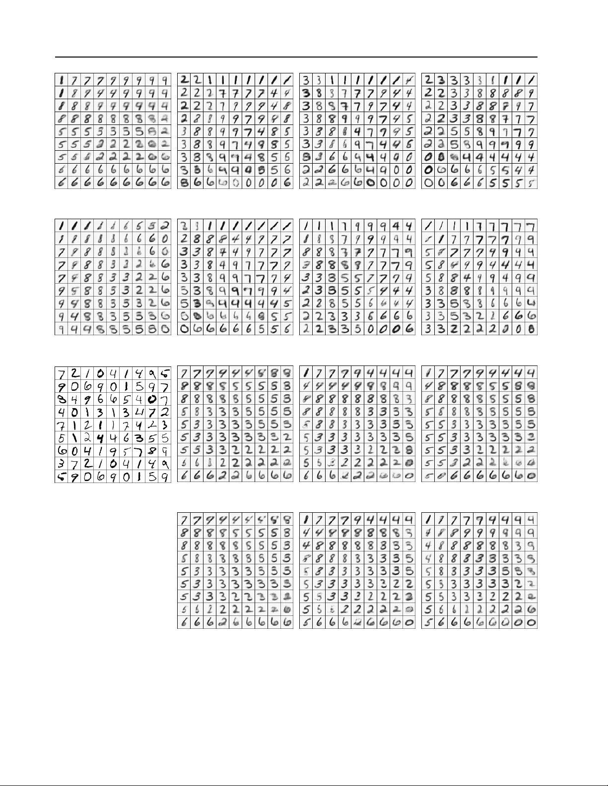
V ariational Learning of Fractional P osteriors Kian Ming A. Chai 1 Edwin V . Bonilla 2 Abstract W e introduce a nov el one-parameter variational objecti ve that lower bounds the data e vidence and enables the estimation of approximate fractional posteriors. W e extend this framework to hierar- chical construction and Bayes posteriors, of fering a versatile tool for probabilistic modelling. W e demonstrate two cases where gradients can be ob- tained analytically and a simulation study on mix- ture models sho wing that our fractional posteriors can be used to achie ve better calibration compared to posteriors from the con ventional v ariational bound. When applied to variational autoencoders (V AEs), our approach attains higher e vidence bounds and enables learning of high-performing approximate Bayes posteriors jointly with frac- tional posteriors. W e show that V AEs trained with fractional posteriors produce decoders that are better aligned for generation from the prior . 1. Introduction Exact Bayesian inference is intractable for most models of interest in machine learning. V ariational methods (Jordan et al., 1999; Minka, 2001; Opper & Winther, 2005; Blei et al., 2017) address this by casting the required integration as optimisation. These methods have two objectives: to estimate the marginal likelihood or data e vidence (MacKay, 2003) for model comparison or model optimisation; and to obtain an approximate Bayes posterior for prediction. The widely used evidence lo wer bound (ELBO) (Jordan et al., 1999) often leads to underestimated uncertainty and suboptimal posterior calibration (W ang & Tittering- ton, 2005; Bishop, 2006; Y ao et al., 2018). These deﬁcien- cies can be compounded by challenges inherent to general Bayesian modelling, such as misspeciﬁcation. Fractional 1 DSO National Laboratories, Singapore 2 CSIR O’ s Data61, Australia. Correspondence to: Kian Ming A. Chai < ckianmin@dso.org.sg > , Edwin V . Bonilla < ed- win.bonilla@data61.csiro.au > . Initial version in Proceedings of the 42 nd International Confer- ence on Machine Learning , V ancouver , Canada. PMLR 267, 2025. Lemma A.1 is corrected here. Copyright 2026 by the author(s). posteriors (Gr ¨ unwald & van Ommen, 2017; Bhattacharya et al., 2019) ha ve emerged as a generalization of Bayesian in- ference to address these. Unlike the Bayes posterior , which fully incorporates the likelihood, a fractional posterior has an exponent that weighs the likelihood to temper its inﬂu- ence. This approach has been shown to enhance rob ustness in misspeciﬁed models and has strong connections to P AC- Bayesian bounds (Bhattacharya et al., 2019), which control generalization error in statistical learning. This work introduces a ne w variational frame work that gen- eralises con ventional variational inference (VI) by allow- ing the approximation of fractional posteriors, enabling im- prov ed posterior ﬂexibility and calibration. As in standard VI based on ELBO maximisation, our approach provides a lo wer bound on the marginal likelihood and extends to hierarchical construction (Ranganath et al., 2016) and Bayes posteriors. Thus it offers a ﬂexible trade-off between evi- dence maximization and posterior calibration, bridging the gap between standard VI and fractional Bayesian inference. W e explore both analytical and empirical insights into vari- ational learning of fractional posteriors. First, we identify cases where gradients can be derived analytically , elim- inating the need for gradient estimators (Roeder et al., 2017). Next, we perform a simulation study on mixture models, demonstrating that fractional posteriors achiev e better-calibrated uncertainties compared to con ventional VI. Finally , we consider v ariational autoencoders (V AEs) (Kingma & W elling, 2014), showing that fractional posteri- ors not only gi ve higher e vidence bounds but also enhance generati ve performance by aligning decoders with the prior— a known issue in standard V AEs (Dai & W ipf, 2019). This work adv ances the ﬁeld of approximate Bayesian infer- ence with a theoretically grounded and empirically validated approach to fractional variational inference. It demonstrates that fractional posteriors can improve model calibration and yield better generati ve models, and it offers an alternati ve to standard variational inference and learning approaches. Notation W e use letter p for model distrib utions and let- ters q and r for approximate distributions. The tilde (˜) accent is for the unnormalised version of the distribution that it modiﬁes; and the asterisk (*) superscript is for the optimised versions. The unaccented letter Z is for the nor - 1 V ariational Learning of Fractional Posteriors malising constant, and ˜ Z is for an arbitrary scaling constant. W e reserve ELBO for the conv entional bound (Jordan et al., 1999). Boldfaces are used only when needed to distinguish vectors from scalars. W e omit the approximate qualiﬁer from appr oximate posterior , unless the conte xt requires it. When comparing evidence bounds, we use the adjective tighter if we can ascertain that the bound is closer to a ﬁxed evidence value; and we use the adjectiv e higher if bounds cannot be compared for tightness because their correspond- ing ﬁxed e vidences are different. The latter is limited to sections 5.2 and 5.3 when we optimise the likelihood of the model. T able 3 in section A lists the bounds in this paper . 2. A Lower Bound with H ¨ older’ s Inequality The log-evidence L evd def = log p ( D ) of data D for a genera- tiv e model in volving an auxillary v ariable z is bounded by the variational R ´ enyi (lo wer) bound L R α (Li & T urner, 2016, Theorem 1) for α > 0 : L evd ≥ L R α def = 1 1 − α log Z q ( z ) ( p ( D, z ) /q ( z )) 1 − α d z . The Kullback-Leibler diver gence (KL, α → 1 ) is the only case where the chain rule of conditional probability holds exactly to get the con ventional ELBO L ELBO def = R q ( z ) log p ( D | z )d z − R q ( z ) log( q ( z ) /p ( z ))d z . This in- volv es the expected log conditional likelihood (ﬁrst term) that encourages data ﬁtting and the KL term between the approximate posterior q ( z ) and the prior p ( z ) (second term) that acts as a regulariser to bias the posterior towards the prior . This decomposition is not possible for other v alues of α , so L R α generally cannot be expressed in such terms. T o this end, we rev ert to the original log-evidence L evd and apply H ¨ older’ s inequality (Rogers, 1888) in the manner of  E  | X | 1 /β  β ≥ E [ | X Y | ] /  E  | Y | 1 /γ  γ , where β + γ = 1 and β , γ ∈ (0 , 1) , with E [ · ] def = Z p ( z ) · d z , X def = p ( D | z ) β , Y def = ˜ q ( z ) /p ( z ) to obtain L evd = 1 β log  Z p ( z ) p ( D | z )d z  β ≥ 1 β log R ˜ q ( z ) p ( D | z ) β d z  R p ( z ) ( ˜ q ( z ) /p ( z )) 1 /γ d z  γ = 1 1 − γ log Z d − γ 1 − γ log Z c def = L γ , (1) where we have expressed β in γ , and we hav e data-ﬁtting and regularisation (comple xity) terms ˜ q d ( z ) def = ˜ q ( z ) p ( D | z ) 1 − γ ˜ q c ( z ) def = ˜ q ( z ) 1 /γ p ( z ) 1 − 1 /γ Z d def = Z ˜ q d ( z )d z Z c def = Z ˜ q c ( z )d z . The deriv ation does not require ˜ q ( z ) to be a distribution. Howe ver Y must be in L γ to apply the H ¨ older’ s inequality , that is, supp ˜ q ⊆ supp p . Hence, the ˜ q must be consistent with the prior p , a desideratum. If ˜ q ( z ) is a distribution q ( z ) , that is, R q ( z )d z = 1 , then the second term of the bound is the R ´ enyi di vergence D 1 /γ [ q ( z ) ∥ p ( z )] . Our objecti ve L γ in eq. (1) can be seen as an example of the generalized variational infer ence framew ork (Knoblauch et al., 2022). Ho wever , it is uniquely deriv ed as a lower bound to the log-evidence, so it naturally encodes the Oc- cam’ s razor principle and can be used for model optimisa- tion (MacKay, 2003, Chapter 28). W e can relate this ob- jectiv e to the con ventional ELBO (Lemma A.3 sho ws that lim γ → 1 L γ = L ELBO using the L ’H ˆ opital’ s rule and the con vergence of R ´ enyi to KL diver gence) and also provide two related bounds (Lemmas A.1 and A.2). 2.1. Fractional Posteriors The optimal L γ is tight at ˜ q ∗ ( z ) = p ( D | z ) γ p ( z ) / ˜ Z , where ˜ Z can be the normalising constant: L ∗ γ = 1 1 − γ log ˜ Z − 1 Z p ( D | z ) p ( z )d z − γ 1 − γ log ˜ Z − 1 /γ Z p ( D | z ) p ( z )d z = log R p ( D | z ) p ( z )d z ≡ L evd . Since L γ is a lower bound, this already pro ves the optimality of ˜ q ∗ (section A.1 giv es a variational deriv ation). In con- trast, the gap between L evd and L R α is the R ´ enyi di vergence D α [ q ( z ) ∥ p ( z | D )] (section A.2), so L R α ’ s optimal q ( z ) is the exact Bayes posterior p ( z | D ) . Nonetheless, L γ is related to L R α by suitable change of distributions (section A.3). The abov e shows that the bound is tight at a fractional pos- terior where the data-likelihood is weighted with γ ∈ (0 , 1) (Bhattacharya et al., 2019). This is more generally kno wn as the Gibbs posterior (Zhang, 1999; Alquier et al., 2016), the power posterior (Friel & Pettitt, 2008), or the tempered posterior (Pitas & Arbel, 2024). As mentioned in the in- troduction, fractional posteriors are related to robustness in misspeciﬁed models (Bhattacharya et al., 2019). W e hav e obtained the fractional posterior directly from op- timising L γ , which allows approximations to the unnor- malised fractional posterior via optimisation within an as- sumed family of non-negati ve functions. It is achie ved without relying on P A C-Bayes or modifying the likelihood, and it follows from optimising a lo wer bound on L evd . It is an alternativ e to the approach by Alquier et al. (2016). 2.2. On the choice of γ It is generally futile to seek a γ ∗ giving the tightest bound: for a giv en probabilistic model and a ﬁxed posterior q , γ ∗ 2 V ariational Learning of Fractional Posteriors depends on q . For , if q is close to the exact Bayes posterior , then γ ∗ = 1 ; if q is close to an exact fractional posterior, then γ ∗ is that fraction. The situation is the same if we learn q within a family Q . If Q contains all the e xact posteriors, Bayes and fractionals, then all values of γ s are optimal because all giv e L evd after optimisation. If, howe ver , Q can approximate only certain fractional posteriors well, then the corresponding γ s will giv e the tightest bounds. Nonetheless, if one applies approximate inference analyt- ically to a problem that is speciﬁed with an explicit prior, such as the normal distribution, it is typical to choose Q to be in the same family as the prior, such that Q includes the prior and its neighbourhood. In this case, we expect optimising with small γ to giv e consistently tighter bounds. This is shown in section 5.1 empirically . In a similar fashion, for challenging data sets for which we use neural networks, we expect smaller γ to give tighter bounds for simpler neural networks that can better approxi- mate the prior and the fractional posteriors than the Bayes posterior . This is supported in section C.4 empirically . Considerations other than bounds may inﬂuence the choice of γ . In section 5.1, we use calibration; in section 5.3, we want a posterior that is close to the prior . 2.3. Extensions to Hierarchical Constructions W e gi ve two extensions to L γ to allow for more e xpressiv e fractional and Bayes posteriors using mixing. W e show in sections A.5.1 and A.5.2 that de generacy of the mixing distribution is not necessary for optimality , in contrast to the case for ELBO (Y in & Zhou, 2018, Proposition 1). 2 . 3 . 1 . F R A C T I O N A L P O S T E R I O R Let ˜ q ( z ) def = R ˜ q ( z | u ) q ( u )d u be a hierarchical model of the posterior distribution using mixing variable u . Jensen’ s inequality for con vexity of po wers above unity gi ves Z c = Z  Z ˜ q ( z | u ) q ( u )d u  1 /γ p ( z ) 1 − 1 /γ d z ≤ Z  Z ˜ q ( z | u ) 1 /γ q ( u )d u  p ( z ) 1 − 1 /γ d z = Z  Z ˜ q ( z | u ) 1 /γ − 1 ˜ q ( z | u ) q ( u )d u  p ( z ) 1 − 1 /γ d z = Z Z ( ˜ q ( z | u ) /p ( z )) 1 /γ − 1 ˜ q ( z | u )d z q ( u )d u (2) W e may substitute this into eq. (1) to obtain another bound, which we shall call L h γ . This lower bound allows Monte Carlo estimates of the integral by only using samples from the posterior ˜ q ( z | u ) (see section 4). A similar approach has been used to lo wer bound the ELBO (Y in & Zhou, 2018, Theorem 1). There, the optimal for q ( u ) is known to be the delta distribution located for opti- mal q ( z | u ) (Y in & Zhou, 2018, Proposition 1). Howe ver , deviations from this property may happen in practice (see sections B.2 and C.4). 2 . 3 . 2 . B AY E S P O S T E R I O R W e can bound the data term in L γ using Jensen’ s inequality with another variational distrib ution r ( z ) : log Z d ≥ (1 − γ ) Z r ( z ) log p ( D | z )d z − Z r ( z ) log r ( z ) ˜ q ( z ) d z so that logarithm o ver the product of lik elihoods becomes a sum ov er the logarithms of each likelihood, and we may sample ov er the data points. Section 3.1.3 giv es a different but more speciﬁc bound for the mixture model. The above bound is exact at r ∗ ( z ) ∝ ˜ q ( z ) p ( D | z ) 1 − γ . If ˜ q ( z ) is also optimal, then r ∗ ( z ) ∝ p ( z ) p ( D | z ) , which is the Bayes posterior . Combining the abov e bound with eq. (1) giv es a bound on L evd in volving both KL and R ´ enyi di ver - gences. W e shall denote this bound by L b γ . If we ﬁx r ( z ) regardless of its optimality , and then optimise for ˜ q ( z ) , we obtain ˜ q ∗ ( z ) ∝ r ( z ) γ p ( z ) 1 − γ interpolating between the ﬁxed r ( z ) and the model prior p ( z ) . This sho ws that r ( z ) has a constraining effect on ˜ q ( z ) , so the fractional posteriors approximated by L b γ are in general dif ferent from those approximated by using L γ . In particular , if r ( z ) itself is a fractional posterior with fraction γ ′ , then ˜ q ( z ) has at best fraction γ ′ γ . This is sho wn empirically in section 5.2.1. For a ﬁxed r ( z ) , L b γ is upper bounded by L ELBO (see Lemma A.4), so L b γ in itself has limited use. Howe ver , we can use it with the hierarchical posterior model (sec- tion 2.3.1) to gi ve more expressi ve posteriors. For this, we hav e to go beyond just applying the hierarchical model on r ( z ) because this will result in a degenerate mixing distri- bution for r ( z ) , since the terms inv olved are exactly the same as in ELBO. T o pre vent degenerac y , we apply hier- archical model to both ˜ q ( z ) and r ( z ) , with the same mix- ing distribution q ( u ) . That is, ˜ q ( z ) def = R ˜ q ( z | u ) q ( u )d u and r ( z ) def = R r ( z | u ) q ( u )d u . Under this setting, we apply eq. (2) on the R ´ enyi di ver gence term and the con vexity on the KL term to obtain a bound we call L bh γ (see section A.4): L evd ≥ Z Z r ( z | u ) q ( u ) log p ( D | z ) d z d u − 1 1 − γ Z Z r ( z | u ) q ( u ) log r ( z | u ) ˜ q ( z | u ) d z d u − γ 1 − γ log Z Z ˜ q ( z | u ) q ( u )  ˜ q ( z | u ) p ( z )  1 /γ − 1 d z d u. 3 V ariational Learning of Fractional Posteriors 3. Learning Let ˜ q be parameterised by θ . Under regularity conditions, ∂ L γ ∂ θ = 1 1 − γ Z ( q d ( z ) − q c ( z )) ∂ log ˜ q ( z ) ∂ θ d z , where q d ( z ) def = ˜ q d ( z ) / Z d and q c ( z ) def = ˜ q c ( z ) / Z c are nor- malised distributions, and we hav e used the log-deriv ativ e trick ∂ log ˜ q /∂ θ = (1 / ˜ q )( ∂ ˜ q /∂ θ ) . At the optimal ˜ q ∗ , both q c ( z ) and q d ( z ) equates the exact Bayes posterior p ( z | D ) . Setting the gradient to zero entails matching the expectations of the gradients of log ˜ q under q c and q d . Gradients for L b γ and L bh γ can be similarly expressed. 3.1. Case Studies W e study three cases of applying L γ analytically . The ﬁrst case where exact inference is possible is illustrative. The other cases, where exact inference is not, demonstrate where using L γ can be useful. 3 . 1 . 1 . E X P O N E N T I A L F A M I L Y Consider D to be a collection of n independent data { x 1 , . . . , x n } in the exponential family with the conju- gate prior setting: p ( x i | z ) = h ( x i ) exp  z T t ( x i ) − a ( z )  ; p ( z | ν , κ ) = g ( ν , κ ) exp  z T ν − κa ( z )  ; and ˜ q ( z | µ , λ ) = exp  z T µ − λa ( z )  , with t being the sufﬁcient statistic, z the natural parameter , a the log-partition function; ν and κ the parameters for the prior; and µ and λ the pa- rameters for the posterior . Then ∂ log ˜ q ( z ) /∂ µ = z and ∂ log ˜ q ( z ) /∂ ν = − a ( z ) , and q c ( z ) ∝ exp  z T ( µ /γ + (1 − 1 /γ ) ν ) − k ( κ ) a ( z ) /γ  q d ( z ) ∝ exp  z T ( µ + (1 − γ ) P n i =1 t ( x i )) − k ( n ) a ( z )  , where k ( • ) def = λ + (1 − γ ) • . The sufﬁcient statistics for conjugate distributions are z and − a ( z ) , so E q c [ z ] = µ /γ + (1 − 1 /γ ) ν E q c [ − a ( z )] = k ( κ ) /γ E q d [ z ] = µ + (1 − γ ) P n i t ( x i ) E q d [ − a ( z )] = k ( n ) . Zeroing gradients ∂ L γ /∂ µ and ∂ L γ /∂ λ giv es the follow- ing parameters for ˜ q as expected: µ = ν + γ P n i =1 t ( x i ) λ = κ + γ n. The parameters interpolate between the prior and the Bayes posterior , as a consequence that exact inference is achiev- able. This is not true for more general models and approxi- mate inference may be required. 3 . 1 . 2 . M U LT I N O M I A L D AT A W I T H G A U S S I A N P R I O R In the previous case where exact posteriors can be obtained, it is not necessary to deri ve the gradients, since we already know the functional form of these posteriors. Where the exact fractional posterior could be complicated, we assume a functional form for the approximate posterior . Consider the model with a multinomial logit likelihood for C classes and a standard Gaussian prior: p ( x | z ) = exp z x P C c =1 exp z c ; p ( z ) = C Y c =1 1 √ 2 π exp − z 2 c 2 . For n data points, we choose 1 /γ = 1 + 1 /n and let ˜ q ( z ) = C Y c =1 N ( z c | µ c , σ 2 c ) ! C X c =1 exp z c ! n/ ( n +1) . Then q c ( z ) ∝  Q C c =1 N ( z c | m c , s 2 c )   P C c =1 exp z c  = P C c =1 exp z c  Q C c ′ =1 N ( z c ′ | m c ′ , s 2 c ′ )  q d ( z ) ∝  Q C c =1 N ( z c | µ c , σ 2 c )  Q n i =1 exp ( z x i / ( n + 1)) ∝ Q C c =1 N  z c | µ c + n c σ 2 c n +1 , σ 2 c  , where m c def = µ c ( n + 1) n + 1 − σ 2 c s 2 c def = nσ 2 c n + 1 − σ 2 c , and n c def = P n i =1 δ ( c, x i ) is the number of data points of class c . The last e xpression of q c has normalising constant P C c =1 exp( m c + s 2 c / 2) , and the last expression for q d is normalised because it is a product of independent Gaussian distributions. The gradients with respect to the parameters and the required expectations are giv en in section A.6. This is an e xample where we need only the unnormalised density ˜ q during optimisation. 3 . 1 . 3 . M I X T U R E M O D E L A common model in the Bayesian literature is the mixture model. For n samples { x i } n i =1 and K components with parameters { u k } K k =1 independently drawn from p ( u k ) , the evidenc e is P c p ( c ) R p ( u ) Q n i =1 p ( x i | c i , u )d u (Blei et al., 2017, Equation 9), where c i ∈ { 1 , . . . , K } is the latent as- signed cluster for the i th sample, and the c i s are independent. The outer sum ov er K n cluster assignments makes exact inference intractable. Assume a mean-ﬁeld approximation for the posterior: q ( u , c ) = Q K k =1 q ( u k ) Q n i =1 q ( c i ) . Like ELBO, we may apply the L b γ bound to con vert the innermost product to an outer sum for the likelihood term. Alternativ ely , we can ﬁrst apply L γ for the variational posterior q ( u ) of the compo- nent means, and then the ELBO for the cluster assignments c , so that the Z d term in eq. (1) is lower bounded by Z q ( u ) n Y i =1 K Y c i =1 ( p ( x i | c i , u ) p ( c i ) /q ( c i )) (1 − γ ) q ( c i ) d u . 4 V ariational Learning of Fractional Posteriors Deﬁne the variational parameters φ ik def = q ( c i = k ) , i = 1 , . . . , n , k = 1 , . . . , K . Simplifying with the mean-ﬁeld independence assumption, the lower bound is (section A.7) K X k =1  1 1 − γ n X i =1 log Z q ( u k ) p ( x i | u k ) (1 − γ ) φ ik d u k − n X i =1 φ ik log ( φ ik /p ( c i = k )) − γ 1 − γ log Z q ( u k ) 1 /γ p ( u k ) 1 − 1 /γ d u k  . Identifying terms with L γ , optimality gi ves q ( u k ) ∝ p ( u k ) Q n i =1 p ( x i | u k ) φ ik γ . For φ ik , we ﬁrst deﬁne distri- butions q i ( u k ) ∝ q ( u k ) p ( x i | u k ) (1 − γ ) φ ik , which introduces the proportion of the i th sample omitted in q ( u k ) . Then φ ik ∝ p ( c i ) exp ( E q i [log p ( x i | u k )]) — in this way , q ( c i ) approximates the Bayes posterior by using the full contri- bution of likelihood due to x i . A full ELBO solution is obtained by setting γ = 1 for the updates; and in particular , q i ( u k ) ≡ q ( u k ) for all i . If each conditional likelihood p ( x i | u k ) is in the exponential family and the prior p ( u k ) is conjugate to it, then q ( u k ) is in the same conjugate family that ha ve the sufﬁcient statistics of the data weighted by φ ik and γ . Consider the Gaussian mixture model of Blei et al. (2017, §2.1), where the com- ponent priors are identically normal with mean zero and variance σ 2 ; the assignment priors are identically uniform; and the likelihood is unit variance normal centered at u k . Then q ( u k ) is normal with mean and v ariance γ P n i =1 φ ik x i 1 /σ 2 + γ P n i =1 φ ik and 1 1 /σ 2 + γ P n i =1 φ ik . The same expressions are obtained from the approxi- mate Bayes posterior r ( u k ) and the prior p ( u k ) using r ( u k ) γ p ( u k ) 1 − γ , but the assignment probabilities φ ik s within are different. Section C.2 illustrates the difference. 4. Monte Carlo Estimates If we ha ve N s samples z i s from distrib ution q ( z ) = ˜ q ( z ) / Z for known normalising constant Z , we can use them to esti- mate Z c and Z d in eq. (1). If we only ha ve the unnormalised density , then estimating L γ requires the normalising factor Z . An alternati ve is to introduce a mixing distrib ution and use the L h γ bound: L h γ ≈ 1 1 − γ log 1 N s P i P j p ( D | z ij ) 1 − γ − γ 1 − γ log 1 N s P i P j ( q ( z ij | u i ) /p ( z ij )) 1 /γ − 1 , where there are no w N ′ s samples from u i ∼ q ( u ) followed by N s / N ′ s samples z ij ∼ q ( z | u i ) . In this setting, ˜ q ( z ) need not be known explicitly , but we are required to be able to draw the ( u i , z i ) s samples and to know the conditional q ( z | u ) exactly . This particular model for q ( z ) is the semi- implicit hierarchical construction (Y in & Zhou, 2018). For L bh γ , we also ha ve N s / N ′ s samples z ′ ik ∼ r ( z | u i ) . Sec- tion B provides more details. 5. Experiments W e provide three e xperiments. The ﬁrst uses analytical up- dates to infer the posteriors for a given model, a variational infer ence task; the second and third, Monte Carlo sampling with the reparameterisation trick (Kingma & W elling, 2014) to infer the posteriors and also learn the hyperparameters of the model, a variational learning task. For γ = 1 . 0 we use the standard ELBO implementation directly . W e refer the reader to T able 3 in section A as a reminder of the bounds used in the paper and ev aluated in this section. 5.1. Calibration Study for Mixtur e Models W e ev aluate the quality of the learnt fractional posteriors by examining the calibration diagnostics for a one-dimensional mixture model. W e use the Gaussian mixture model (GMM) of Blei et al. (2017, §2.1), where each observation is drawn with white noise (that is, variance σ 2 obs = 1 ) from one of the K components with equal probability , and the component means hav e independent and identical Gaussian priors. W e infer posteriors over component means using v ariational inference on a set of observ ations. For a gi ven signiﬁcance lev el α , actual cov erage is the long-term frequency that the 1 − α credible interval from a posterior includes the true component mean. The credible interval is calibrated when the actual coverage is 1 − α . It is known that the posteriors from ELBO are overconﬁdent (W ang & Titterington, 2005). W e use K = 2 components centered at µ 1 = − 2 and µ 2 = 2 , and we compute the empirical coverage κ ov er 5 , 000 repli- cas of n = 400 observations (Syring & Martin, 2019, §S2). For each replica, we obtain the approximate fractional pos- teriors for γ = 0 . 1 to 0 . 9 in intervals of 0.1, and the ap- proximate Bayes posterior using ELBO (see section 3.1.3). Using α = 0 . 05 , we ﬁnd that the posteriors from ELBO and γ = 0 . 9 are overconﬁdent, that is, κ < 1 − α ; and those from γ ≤ 0 . 8 are conservati ve (ﬁrst set of results in T able 1). Moreov er, the interv al lengths ℓ s decrease with γ . These ﬁndings conform to our expectations of fractional posteriors, and they demonstrate that optimising L γ giv es approximate fractional posteriors with the intended properties. T o see the ef fect of the interval length ℓ on κ , we measure the cov erages when, for each replica, the component means are from the Bayes posterior b ut the component v ariances are from fractional posteriors with γ = 0 . 1 , 0 . 5 or 0 . 9 . W e ﬁnd the coverages for such conﬂated models C γ s match that 5 V ariational Learning of Fractional Posteriors T able 1: Calibration study of GMM at α = 0 . 05 signif- icance. The empirical cov erages κ (higher is better) and av erage interval lengths ℓ (shorter better) for each of the { µ 1 , µ 2 } means are shown. The last column giv es the bounds to L evd (higher better). The ﬁrst set of results is from modelling with different γ s ( L 1 . 0 is ELBO). Results for γ ∈ { 0 . 2 , 0 . 4 , 0 . 6 , 0 . 8 } are omitted for brevity , but the trend remains. The second set is from conﬂated models combining the means from ELBO and the variances from L γ . The third set is from calibrations of using the ﬁrst set of results. The γ v alues for R ℓ and R κ are 0 . 785 and 0 . 798 . µ 1 µ 2 κ ℓ κ ℓ bound L 0 . 1 1 . 0000 0 . 8515 1 . 0000 0 . 8987 − 832 . 5 L 0 . 3 0 . 9994 0 . 4924 0 . 9988 0 . 5200 − 833 . 3 L 0 . 5 0 . 9876 0 . 3816 0 . 9860 0 . 4029 − 834 . 0 L 0 . 7 0 . 9694 0 . 3225 0 . 9606 0 . 3406 − 834 . 4 L 0 . 9 0 . 9438 0 . 2845 0 . 9334 0 . 3004 − 834 . 8 L 1 . 0 0 . 9278 0 . 2699 0 . 9182 0 . 2850 − 834 . 9 C 0 . 1 1 . 0000 0 . 8515 1 . 0000 0 . 8987 − 839 . 3 C 0 . 5 0 . 9878 0 . 3816 0 . 9858 0 . 4029 − 834 . 5 C 0 . 9 0 . 9436 0 . 2845 0 . 9334 0 . 3004 − 834 . 8 R ℓ 0 . 9588 0 . 3046 0 . 9474 0 . 3216 − 834 . 6 R κ 0 . 9570 0 . 3021 0 . 9458 0 . 3190 − 834 . 6 of the corresponding fractional posteriors in general, but for a minority of replicas changing the variances is insuf ﬁcient (compare the cov erages of C γ s to L γ s in T able 1). Here, we inv estigate two calibration strategies, one using interval lengths ℓ s and the other using cov erages κ s. Gi ven our knowledge of the model, sans the locations of the com- ponents, we expect n/K observations per component, so their sample mean has v ariance K σ 2 obs /n . Combining this with the critical value for α provides an interval length ℓ ∗ that we expect in the ideal case. F or each r eplica and each component k , we perform linear regression on γ against ℓ using the results from L γ to predict γ ∗ k at ℓ ∗ . W e a verage the γ ∗ k s to obtain γ ∗ for that replica. The model that optimises L γ ∗ in then computed, for each replica. W e call this R ℓ . The other strategy , called R κ , has to be performed after computing the κ s ov er the replicas. This regresses linearly γ against κ using the results from L γ to predict the γ ∗ k at 1 − α cov erage, for each component k . W e then obtain a single γ ∗ by av eraging the γ ∗ k s. For each replica, the model that optimises L γ ∗ is then computed. In this study , we ﬁnd both R ℓ and R κ to provide co verages close to 1 − α (last set of results in T able 1). For R ℓ , the av erage value of γ ∗ is 0 . 78 , while for R κ the value is 0 . 80 . In practice, when replications of data sets are not a vailable, bootstrapping can be used (Syring & Martin, 2019). Both R ℓ and R κ are shown to be effecti ve, and which to use in practice will depend primarily on the nature of data collec- tion. Section C.1 giv es additional examples; here we note that analysis for K > 2 components is complicated by the complex mar ginal likelihood landscape (Jin et al., 2016). Bounds W ith current experimental settings, we perform importance sampling using 1,000 samples to estimate the log-evidence to be − 827 . 2 . So, while L 0 . 1 is the tightest (last column in T able 1) in this scenerio, it is still rather loose. Section C.3 provides more details. 5.2. V ariational A utoencoder V ariational autoencoder (V AE) (Kingma & W elling, 2014) provides a variational objective to learn the the encoder and decoder neural networks of an autoencoder . Though there are man y variations (for example, T omczak & W elling (2018); Higgins et al. (2017)), we compare with the standard V AE since our aim is to inv estigate differences with ELBO. V AE is a local latent variable model that separately applies ELBO to each datum. This will be the same for our bounds. W e follow the experimental setup and the neural network models of Ruthotto & Haber (2021) for the gray-scale MNIST dataset (Lecun et al., 1998). The latent space is two-dimensional, so we can inspect the posteriors visually . W e make three changes (see section C.4): most signiﬁcantly we use the continuous Bernoulli distribution (Loaiza-Ganem & Cunningham, 2019) as the likelihood function. W e use four values of γ s: 1.0 (ELBO), 0.9, 0.5 and 0.1. For the posterior family , we use an explicit normal dis- tribution (following Ruthotto & Haber (2021)) and also a semi-implicit distrib ution. For the latter we use a three-layer neural network for the implicit distrib ution, similar to that used by Y in & Zhou (2018) (details in section C.4). The choice of posterior family af fects only the encoder structure. In V AE, the log-evidence L evd depends on the prior and the likelihood, which in turn depends on the learnt V AE decoder . Hence, optimising the decoder par ameters can be seen as an ML-II pr ocedur e (W ang et al., 2019). Therefore, when comparing the e vidence bounds after optimisation, we can only say that the optimised models pro vide certain guaran- tees on L evd , with higher bounds gi ving better guarantees. For tightness of bounds, see section C.4 (T able 7). W e ﬁrst look at the effect of γ and posterior families, and where L γ uses the explicit distributions and L h γ uses the semi-implicit distributions. While the learning objectiv es are on the training set, we also examine them on the test set to assess generalisation. W e observe smaller γ s gi ves higher ﬁnal evidence bounds (third and fourth columns of T able 2, 6 V ariational Learning of Fractional Posteriors T able 2: A verage log-evidences (higher better) over data samples, and its breakdown for V AE on MNIST data sets. W e giv e the mean and three standard de viations of these averages o ver ten experimental runs. For Monte Carlo a verages, 1,024 samples are used ( 32 × 32 for semi-implicit posteriors). For γ = 1 . 0 , the ﬁgures are the same under T est using Objective and T est using ELBO . For the ﬁrst eight rows, the columns under T est using ELBO are solely for diagnostics to understand the learnt posteriors using the same metrics: they are not performance measures. For L bh γ , we sho w the addition of the KL div ergence and R ´ enyi di vergence for T est using Objective ; and for T est using ELBO we ev aluate the Bayes posterior r . T est using Objectiv e T est using ELBO Objectiv e γ Train (T otal) T otal data div T otal data div L γ 1.0 1614 . 3 ± 11 . 0 1583 . 2 ± 14 . 6 1588 . 5 ± 14 . 5 5 . 3 ± 0 . 2 1583 . 2 ± 14 . 6 1588 . 5 ± 14 . 5 5 . 3 ± 0 . 2 0.9 1648 . 5 ± 5 . 1 1639 . 3 ± 4 . 5 1641 . 9 ± 4 . 8 2 . 6 ± 0 . 4 1452 . 6 ± 48 . 0 1455 . 0 ± 48 . 0 2 . 4 ± 0 . 3 0.5 1675 . 9 ± 5 . 0 1672 . 8 ± 5 . 9 1674 . 7 ± 6 . 0 1 . 9 ± 0 . 3 1318 . 7 ± 42 . 1 1320 . 1 ± 42 . 2 1 . 4 ± 0 . 2 0.1 1680 . 1 ± 2 . 9 1677 . 2 ± 3 . 4 1679 . 5 ± 3 . 4 2 . 3 ± 0 . 3 1322 . 8 ± 49 . 0 1324 . 2 ± 49 . 1 1 . 3 ± 0 . 2 L h γ 1.0 1639 . 6 ± 14 . 6 1609 . 6 ± 20 . 6 1614 . 6 ± 20 . 5 5 . 0 ± 0 . 3 1609 . 7 ± 20 . 6 1614 . 6 ± 20 . 5 5 . 0 ± 0 . 3 0.9 1657 . 7 ± 6 . 1 1647 . 8 ± 5 . 6 1651 . 1 ± 5 . 6 3 . 3 ± 0 . 3 1534 . 6 ± 57 . 0 1537 . 8 ± 57 . 1 3 . 2 ± 0 . 3 0.5 1677 . 4 ± 4 . 1 1674 . 4 ± 5 . 0 1676 . 4 ± 5 . 0 2 . 1 ± 0 . 2 1366 . 0 ± 62 . 0 1367 . 7 ± 62 . 2 1 . 7 ± 0 . 2 0.1 1681 . 4 ± 2 . 7 1678 . 7 ± 3 . 1 1681 . 2 ± 3 . 2 2 . 5 ± 0 . 2 1355 . 6 ± 37 . 7 1357 . 1 ± 37 . 8 1 . 6 ± 0 . 2 L bh γ 0.9 1636 . 2 ± 11 . 5 1608 . 8 ± 23 . 3 1613 . 4 ± 23 . 0 4 . 0 ± 0 . 2 + 0 . 6 ± 0 . 3 1607 . 7 ± 23 . 9 1613 . 4 ± 23 . 0 5 . 7 ± 1 . 0 0.5 1635 . 2 ± 10 . 5 1608 . 0 ± 25 . 4 1612 . 7 ± 25 . 2 4 . 3 ± 0 . 2 + 0 . 4 ± 0 . 2 1607 . 4 ± 25 . 8 1612 . 7 ± 25 . 3 5 . 3 ± 0 . 6 0.1 1635 . 5 ± 12 . 0 1607 . 5 ± 16 . 1 1612 . 4 ± 16 . 1 4 . 6 ± 0 . 1 + 0 . 3 ± 0 . 2 1607 . 3 ± 16 . 2 1612 . 4 ± 16 . 1 5 . 1 ± 0 . 2 ﬁrst two sets of results), showing that L γ and L h γ can be better than L ELBO . This implies that using a range of γ s is useful for model selection, comparison and optimisation. Moreov er, L 0 . 9 with the simpler e xplicit posterior already giv es higher bound than L h 1 . 0 (ELBO) with the semi-implicit posterior (compare their fourth columns), illustrating that γ is more impactful than the posterior family . Nonethe- less, for the same γ , the semi-implicit posterior family gi ves higher evidence bounds (compare the ﬁrst two sets of re- sults), showing that L h γ is a viable approach to learning within the semi-implicit family . The R ´ enyi and KL div ergences generally increase with γ (sixth and ninth columns in T able 2). In particular, the trend for KL validates that we are learning fractional posteriors closer to the prior for smaller γ s. The means of the explicit posterior distributions have also less spread for smaller γ s (see Fig. 4 in section C); samples from these distributions, which depends on the learnt variances, also demonstrate the same (Fig. 5, section C). This also means that the data is less ﬁtted for smaller γ s, which is generally sho wn from the data ﬁt term in ELBO (eighth column in T able 2). There are more clumps in samples from the semi-explicit posteriors than from the explicit ones (Fig. 5, section C), demonstrating the mixing property of the former . The sam- ples from the implicit posteriors shows that the implicit distribution for γ = 1 . 0 (ELBO) are mostly concentrated (Fig. 6a, section C), suggesting frequent de generacy to the delta distribution, in broad agreement to theory (Y in & Zhou, 2018). In contrast, those for γ < 1 , we ﬁnd diverse samples in most cases (Figs. 6b to 6d). This demonstrates that learn- ing with our bounds is a viable alternative to other methods (Y in & Zhou, 2018; T itsias & Ruiz, 2019; Uppal et al., 2023) to prev ent collapse of the implicit distributions. Because of the degenerac y of hierarchical posterior for the ELBO, we have expected to ﬁnd the results of L h 1 . 0 to be very similar to that of L 1 . 0 . Howe ver , this is not the case here. W e postulate that the different gradients and the ad- ditional implicit samples ha ve led to dif ferent learning dy- namics and allow L h 1 . 0 to escape local optimas in the neural network parameter space. The large variances in the train objectiv es across the ten experimental runs support this. Bounds For a limited comparison on the tightness of the bounds with respect to a common L evd , we take a single run of L ELBO for the explicit posterior and uses its decoder as the ﬁx ed decoder to train the encoders (or posteriors) for L γ . W ith smaller γ s, we obtain tighter bounds and posteriors closer to the prior . Details are in section C.4. 5 . 2 . 1 . C O M PA R I N G L bh γ W I T H L h γ W e examine the joint learning of Bayes posterior r and a fractional posterior q using the bound L bh γ , where the posteriors are in the same semi-implicit f amily . W e compare with using L h γ , in both the bounds and the posteriors. The neural network settings are the same as for L h γ . The train and test objectives of L bh γ do not perform better than those from L h γ (and L γ for γ  = 1 . 0 ; last three ro ws in 7 V ariational Learning of Fractional Posteriors (a) Random test samples (b) L γ , γ = 1 ; or ELBO (c) L γ , γ = 10 − 5 (d) Prior distribution Figure 1: W e train V AEs on the Fashion-MNIST dataset using L γ for different γ s. W e obtain mean images from the decoding latent variables that are systematically sampled by coordinate-wise inv erse-CDF (standard normal) transform from a unit square. Fig. b shows the images using the Bayes posterior (learnt with ELBO), and Fig. c sho ws those using a fractional posterior very close to the prior . The last image is the heat map of the corresponding prior densities. T able 2), ev en though there are more parameters — those for the Bayes posterior r . In particular , they do not perform better than L h 1 . 0 , as would be suggested by Lemma A.4; but we qualify that the decoders and hence the probabilistic models are probably different. W e ﬁnd KL[ r ∥ q ] to be lar ge, and it increases with smaller γ , as expected (ﬁrst summand in the sixth column in T able 2). When we e valuate the Bayes posteriors r s with ELBO, we ﬁnd that the y are competiti ve with those obtained by directly optimising L h 1 . 0 (sev enth column). Comparing the R ´ enyi di vergences of the fractional posteri- ors learnt with L bh γ to those learnt with L h γ (sixth column in T able 2), we ﬁnd those learnt with L bh γ signiﬁcantly closer to the prior . This sho ws that the fractional posteriors from L bh γ are constrained signiﬁcantly by the Bayes posteriors when learnt jointly (see third paragraph in section 2.3.2). 5.3. Impro ving V AE Decoder via Fractional Posteriors The decoder of V AE is learnt with latent samples from the encoder . An encoder from a fractional posterior gives samples closer to the prior than the Bayes posterior . Hence, when we generate images from the V AE decoder using samples from the prior—that is, without using the encoder that need an input data—we expect the decoder learnt with a smaller γ to provide better images. W e illustrate this with the Fashion-MNIST dataset (Xiao et al., 2017), training with L γ for γ taking values 1 . 0 (for Bayes posterior), 10 − 1 , 10 − 3 and 10 − 5 (for fractional poste- rior close to prior). Using latent samples from the prior, the decoder trained with the Bayes posterior provides images that are of lower quality then the decoder trained with the fractional posterior with γ = 10 − 5 (Fig. 1; and Fig. 7 in section C.5). T o quantify , we generate 10,000 images from each trained decoder and measure their Fr ´ echet inception distances (FIDs, Heusel et al. 2017; Seitzer 2020) to the test set: with decreasing γ , the distances are 83.5, 69.5, 67.8 and 68.8 (smaller is better). This sho ws that fractional posteriors can train better decoders for generativ e modelling. The β -V AE objective (Higgins et al., 2017) with the appro- priate parameters also giv es fractional posteriors. Howe ver , this objectiv e can be unstable during optimisation, espe- cially when we seek fractional posteriors v ery close to the prior . For the same fractional posteriors with γ set to 10 − 1 , 10 − 3 and 10 − 5 , we obtain FIDs 77.3, 334.7 and 342.3. Sec- tion C.5 provides the details. 6. Related W ork Generalised variational infer ence (Knoblauch et al., 2022) provides an optimisation frame work that generalises ELBO. Being generic, one need to concretise the individual terms before applying to speciﬁc cases. One example is β -V AE (Higgins et al., 2017) for learning disentangled represen- tations in variational autoencoders (V AEs): it weighs the div ergence term more heavily . By construction, the β -V AE bound is prov ably not tighter than ELBO, and optimising it gi ves a fractional posterior . The importance weighted ELBO is also not tighter than ELBO (Domke & Sheldon, 2018, eq. 8). In contrast, the variational R ´ enyi bound (Li & T urner, 2016) can be tighter than ELBO, and optimising it giv es the Bayes posterior . This paper provides a bound that can be better than ELBO, especially for simpler assumed family of distrib utions, and optimising it giv es a fractional posterior . W e show this with the calibration and V AE study . In a standard V AE, the decoder is trained with samples from the posteriors encoded using the training data, but these are unav ailable for pure generative tasks. Current approaches ov ercome this by learning a prior that is accessible during generation, with the objecti ve for matching the prior to 8 V ariational Learning of Fractional Posteriors the posteriors (Makhzani et al., 2016; T omczak & W elling, 2018; Tran et al., 2021). The alternativ e is to train the decoder via a distribution close to the prior . While the β - V AE implies such a distrib ution, its looser bound suggests that the decoder parameters may be learnt suboptimally . Our approach uses fractional posteriors and gives bounds higher than ELBO empirically . V ariational inference can be seen as intentional model mis- speciﬁcation (Chen et al., 2018). Fractional posteriors is one approach to overcome misspeciﬁcation (Gr ¨ unwald & van Ommen, 2017). Such posteriors can be obtained by sampling with down-weighted likelihood; or one can adjust the scale parameter of the Bayes posterior (Syring & Martin, 2019). Alternativ ely , one can optimise the β -V AE objec- tiv e (Alquier et al., 2016; Higgins et al., 2017). W e have provided an alternati ve variational approach to approximate fractional posteriors, and we have demonstrated calibration using them within regression procedures. More complex calibration procedures (Gr ¨ unwald & van Ommen, 2017; Syring & Martin, 2019) can be explored. 7. Discussions and Limitations Misspeciﬁcation If the prior and likelihood are correctly giv en, and if exact inference is possible, then in principle a Bayesian only needs to compute the e xact Bayes posterior . This seldom happens in practice (F aden & Rausser, 1976). If either the prior or likelihood or both are misspeciﬁed, then post-Bayesianism efforts, such as generalised Bayes (Knoblauch et al., 2022), rob ust Bayesian (Miller & Dunson, 2019) and P AC-Bayes (Mase gosa, 2020; Morningstar et al., 2022), seek to ameliorate the situation. This paper does not directly address the goals of post-Bayesianism. It has not ev aluated when either the likelihood or the prior is misspec- iﬁed. Although those for MNIST and F ashion-MNIST are most probably misspeciﬁed, we have not compared to when they are not. W e rely on the works of others to address such goals. Nonetheless, we make a two connections here. First, using fractional posteriors is a proposed solution for misspeciﬁcation (Gr ¨ unwald & van Ommen, 2017; Bhat- tacharya et al., 2019; Medina et al., 2022), and our ob- jectiv e does this naturally through a lower bound on the log-evidence. While the objectiv e is not as intuitiv e as, say , the β -V AE objective, a lower bound like L γ that can be tighter than ELBO can help in selecting or optimising appro- priately parameterised priors in an empirical Bayes manner (Berger & Berliner, 1986). Second, our objectiv e uses the R ´ enyi di vergence to quantify the closeness of the prior to the posterior , and this di vergence is well-beha ved for robustness to prior misspeciﬁcation (Knoblauch et al., 2022, §5.2.1). When exact inference is not possible, we can use approxi- mate inference by way of variational optimisation, which is the main alternati ve to Monte Carlo approaches. When the assumed v ariational family does not include the e xact Bayes posterior , some—but not all—also consider this misspeci- ﬁcation (Chen et al., 2018; Knoblauch et al., 2022). This paper addresses this by e xpanding the possibility afforded by the con ventional ELBO, so that we may also have ap- proximate fractional posteriors as the optimal solutions. At this point, there is no single recipe to select γ (section 2.2); we opine that this should be application dependent. For e x- ample in section 5.1, the best γ s are selected for calibration and not for the tightness of the corresponding bounds. Posterior collapse W ith small γ , we might seem to be en- couraging posterior collapse (W ang et al., 2021). Howe ver , Fig. 4d for γ = 0 . 1 demonstrates that while the fractional posteriors as a whole aggre gate tow ards the prior , the pos- terior for e very data point is dif ferent. This topic demands more in vestigation and discussion than possible here. Limitations W e identify three limitations with L γ . First, the con ventional ELBO using the KL di vergence is usually more mathematically elegant and con venient. This is be- cause it can con vert a log-sum (or log-inte gral) to a sum-log (or integral-log), and a sum or integral is neccessary for marginalisation. In particular , the variational inference for the mixture model must rely on the ELBO at some point (section 3.1.3). Second, the R ´ enyi div ergence is ﬁnite in less cases than the KL (Gil et al., 2013). It may be necessary to consider this when optimising the parameters of the approx- imate posteriors, though we ha ve not needed to do this for the presented experiments. Third, when using Monte Carlo estimates, more than one sample is required to be ef fectiv e (section B.1). This can be unrealistic for huge datasets. Po wer posteriors This paper focuses on estimating an approximate fractional posteriors with the lower bound L γ on the log-e vidence. For power posteriors with γ > 1 , we also hav e lower bounds (Lemma A.1). Similarly , there is no ﬁxed criterion to select such γ s (section 2.2). Estimat- ing these posteriors in volves maximising the lo wer bounds, which should be achiev able by methods presented here. 8. Conclusions W e hav e presented a novel one-parameter v ariational lower bound for the evidence. Maximising the bound within an assumed family of distributions estimates approximate frac- tional posteriors. W e have given analytical updates for ap- proximate inference in two intractable models. Empirical results for calibration and V AE show the utility of our ap- proach. For the Fashion-MNIST dataset, V AE decoders learnt with our approach can generate better images. 9 V ariational Learning of Fractional Posteriors Acknowledgements W e thank Xuesong W ang and Rafael Oliv eira for their inputs, and the revie wers for their constructive comments. This research was conducted while Chai was visiting CSIR O’ s Data61, and the Machine Learning and Data Science Unit in the Okinawa Institute of Science and T echnology (OIST). Impact Statement This paper presents work whose goal is to advance the ﬁeld of Machine Learning. There are many potential societal consequences of our work, none which we feel must be speciﬁcally highlighted here. References Alquier , P ., Ridgway , J., and Chopin, N. On the properties of variational approximations of Gibbs posteriors. Journal of Machine Learning Resear ch , 17(236):1–41, 2016. Berger , J. and Berliner , L. M. Robust Bayes and empirical Bayes analysis with ϵ -contaminated priors. The Annals of Statistics , 14(2):461–486, 1986. Bhattacharya, A., Pati, D., and Y ang, Y . Bayesian fractional posteriors. The Annals of Statistics , 47(1):39–66, 2019. Bishop, C. M. P attern Recognition and Machine Learning (Information Science and Statistics) . Springer-V erlag, Berlin, Heidelberg, 2006. ISBN 0387310738. Blei, D. M., Kucukelbir , A., and McAulif fe, J. D. V aria- tional inference: A revie w for statisticians. Journal of the American Statistical Association , 112(518):859–877, 2017. Chen, Y .-C., W ang, Y . S., and Eroshev a, E. A. On the use of bootstrap with v ariational inference: Theory , interpre- tation, and a two-sample test example. The Annals of Applied Statistics , 12(2):846–876, 2018. Dai, B. and W ipf, D. Diagnosing and enhancing V AE mod- els. In International Conference on Learning Repr esenta- tions , 2019. Domke, J. and Sheldon, D. R. Importance weighting and variational inference. In Bengio, S., W allach, H., Larochelle, H., Grauman, K., Cesa-Bianchi, N., and Gar- nett, R. (eds.), Advances in Neural Information Pr ocess- ing Systems , volume 31. Curran Associates, Inc., 2018. Faden, A. M. and Rausser , G. C. Econometric policy model construction: The post-Bayesian approach. Annals of Economic and Social Measur ement , 5(3):349–362, 1976. Friel, N. and Pettitt, A. N. Marginal likelihood estimation via power posteriors. J ournal of the Royal Statistical Society Series B: Statistical Methodology , 70(3):589–607, 2008. Gelman, A. and Meng, X.-L. Simulating normalizing con- stants: from importance sampling to bridge sampling to path sampling. Statistical Science , 13(2):163–185, 1998. Gil, M., Alajaji, F ., and Linder , T . R ´ enyi di vergence mea- sures for commonly used univ ariate continuous distribu- tions. Information Sciences , 249:124–131, 2013. Gr ¨ unwald, P . and v an Ommen, T . Inconsistency of Bayesian inference for misspeciﬁed linear models, and a proposal for repairing it. Bayesian Analysis , 12(4):1069–1103, 2017. doi: 10.1214/17- BA1085. Heusel, M., Ramsauer , H., Unterthiner, T ., Nessler , B., and Hochreiter , S. GANs trained by a two time-scale update rule con verge to a local Nash equilibrium. In Pr oceedings of the 31st International Confer ence on Neural Informa- tion Pr ocessing Systems , pp. 6629–6640, Red Hook, NY , USA, 2017. Curran Associates Inc. Higgins, I., Matthey , L., Pal, A., Bur gess, C. P ., Glorot, X., Botvinick, M. M., Mohamed, S., and Lerchner , A. β - V AE: Learning basic visual concepts with a constrained variational frame work. In International Confer ence on Learning Repr esentations , 2017. Jin, C., Zhang, Y ., Balakrishnan, S., W ainwright, M. J., and Jordan, M. I. Local maxima in the likelihood of Gaus- sian mixture models: structural results and algorithmic consequences. In Pr oceedings of the 30th International Confer ence on Neural Information Pr ocessing Systems , NIPS’16, pp. 4123–4131, Red Hook, NY , USA, 2016. Curran Associates Inc. Jordan, M. I., Ghahramani, Z., Jaakkola, T . S., and Saul, L. K. An introduction to variational methods for graphical models. Machine Learning , 37(2):183–233, 1999. Kingma, D. P . and W elling, M. Auto-encoding variational Bayes. In International Confer ence on Learning Repr e- sentations , 2014. Knoblauch, J., Jewson, J., and Damoulas, T . An optimization-centric view on Bayes’ rule: Revie wing and generalizing variational inference. Journal of Machine Learning Resear ch , 23(132):1–109, 2022. Lecun, Y ., Bottou, L., Bengio, Y ., and Haffner , P . Gradient- based learning applied to document recognition. Pr oceed- ings of the IEEE , 86(11):2278–2324, 1998. Li, Y . and T urner , R. E. R ´ enyi div ergence v ariational in- ference. In Advances in Neural Information Pr ocessing Systems , volume 29, pp. 1081–1089, 2016. 10 V ariational Learning of Fractional Posteriors Loaiza-Ganem, G. and Cunningham, J. P . The continuous Bernoulli: ﬁxing a perv asiv e error in variational autoen- coders. In Advances in Neural Information Pr ocessing Systems , volume 32, 2019. Maas, A. L., Hannun, A. Y ., and Ng, A. Y . Rectiﬁer non- linearities improve neural network acoustic models. In ICML W orkshop on Deep Learning for Audio, Speech, and Language Pr ocessing (WDLASL 2013) , 2013. MacKay , D. J. C. Information theory , infer ence and learning algorithms . Cambridge University Press, 2003. Makhzani, A., Shlens, J., Jaitly , N., and Goodfellow , I. Adversarial autoencoders. In International Conference on Learning Repr esentations (W orkshop T rack) , 2016. Masegosa, A. Learning under model misspeciﬁcation: Applications to v ariational and ensemble methods. In Larochelle, H., Ranzato, M., Hadsell, R., Balcan, M., and Lin, H. (eds.), Advances in Neural Information Pr ocess- ing Systems , volume 33, pp. 5479–5491. Curran Asso- ciates, Inc., 2020. Medina, M. A., Olea, J. L. M., Rush, C., and V elez, A. On the robustness to misspeciﬁcation of α -posteriors and their variational approximations. Journal of Machine Learning Resear ch , 23(147):1–51, 2022. Miller , J. W . and Dunson, D. B. Robust Bayesian infer- ence via coarsening. Journal of the American Statistical Association , 114(527):1113–1125, 2019. Minka, T . P . Expectation propagation for approximate Bayesian inference. Uncertainty in Artiﬁcial Intelligence, pp. 362–369, San Francisco, CA, USA, 2001. Morgan Kaufmann Publishers Inc. ISBN 1558608001. Morningstar , W . R., Alemi, A., and Dillon, J. V . P A C m - Bayes: Narrowing the empirical risk gap in the misspeci- ﬁed Bayesian regime. In Camps-V alls, G., Ruiz, F . J. R., and V alera, I. (eds.), Pr oceedings of The 25th Interna- tional Conference on Artiﬁcial Intelligence and Statis- tics , volume 151 of Pr oceedings of Machine Learning Resear ch , pp. 8270–8298. PMLR, 2022. Opper , M. and Winther , O. Expectation consistent approxi- mate inference. Journal of Machine Learning Researc h , 6(73):2177–2204, 2005. Pitas, K. and Arbel, J. The ﬁne print on tempered posteriors. In Pr oceedings of the 15th Asian Confer ence on Machine Learning , volume 222 of Pr oceedings of Machine Learn- ing Resear ch , pp. 1087–1102. PMLR, 2024. Ranganath, R., T ran, D., and Blei, D. Hierarchical varia- tional models. In Balcan, M. F . and W einberger , K. Q. (eds.), Pr oceedings of The 33rd International Confer ence on Machine Learning , v olume 48 of Pr oceedings of Ma- chine Learning Resear ch , pp. 324–333, Ne w Y ork, New Y ork, USA, 20–22 Jun 2016. PMLR. Roeder , G., W u, Y ., and Duvenaud, D. Sticking the landing: Simple, lo wer-v ariance gradient estimators for variational inference. In Advances in Neural Information Pr ocessing Systems , volume 30, pp. 6925–6934, 2017. Rogers, L. J. An extension of a certain theorem in inequali- ties. Messenger of Mathematics, Ne w Series , XVII(10): 145–150, 1888. Ruthotto, L. and Haber , E. An introduction to deep genera- tiv e modeling. GAMM-Mitteilungen , 44(2):e202100008, 2021. Seitzer , M. pytorch-ﬁd: FID Score for PyT orch. https:// github.com/mseitzer/pytorch- fid , August 2020. V ersion 0.3.0. Syring, N. and Martin, R. Calibrating general posterior credible regions. Biometrika , 106(2):479–486, 2019. T itsias, M. K. and Ruiz, F . Unbiased implicit variational inference. In Pr oceedings of the T wenty-Second Interna- tional Confer ence on Artiﬁcial Intelligence and Statistics , volume 89 of Pr oceedings of Machine Learning Resear ch , pp. 167–176, 2019. T omczak, J. M. and W elling, M. V AE with a V ampPrior . In Storke y , A. J. and P ´ erez-Cruz, F . (eds.), International Confer ence on Artiﬁcial Intelligence and Statistics, AIS- T A TS 2018, 9-11 April 2018, Playa Blanca, Lanzar ote, Canary Islands, Spain , volume 84 of Pr oceedings of Ma- chine Learning Resear ch , pp. 1214–1223. PMLR, 2018. T ran, B.-H., Rossi, S., Milios, D., Michiardi, P ., Bonilla, E. V ., and Filippone, M. Model selection for Bayesian autoencoders. In Ranzato, M., Beygelzimer , A., Dauphin, Y ., Liang, P ., and V aughan, J. W . (eds.), Advances in Neural Information Pr ocessing Systems , volume 34, pp. 19730–19742. Curran Associates, Inc., 2021. Uppal, A., Stensbo-Smidt, K., Boomsma, W ., and Frellsen, J. Implicit variational inference for high-dimensional posteriors. In Advances in Neural Information Pr ocessing Systems , volume 36, pp. 73793–73816, 2023. van Erven, T . and Harremos, P . R ´ enyi div ergence and Kullback-Leibler di vergence. IEEE T ransactions on In- formation Theory , 60(7):3797–3820, 2014. W ang, B. and T itterington, D. M. Inadequacy of interval estimates corresponding to v ariational Bayesian approx- imations. In Cowell, R. G. and Ghahramani, Z. (eds.), 11 V ariational Learning of Fractional Posteriors Pr oceedings of the T enth International W orkshop on Arti- ﬁcial Intelligence and Statistics , v olume R5 of Pr oceed- ings of Machine Learning Resear ch , pp. 373–380. PMLR, 06–08 Jan 2005. W ang, Y ., Miller , A. C., and Blei, D. M. Comment: V aria- tional autoencoders as empirical Bayes. Statistical Sci- ence , (2):229–233, 2019. W ang, Y ., Blei, D., and Cunningham, J. P . Posterior collapse and latent variable non-identiﬁability . In Ranzato, M., Beygelzimer , A., Dauphin, Y ., Liang, P ., and V aughan, J. W . (eds.), Advances in Neural Information Pr ocessing Systems , volume 34, pp. 5443–5455. Curran Associates, Inc., 2021. Xiao, H., Rasul, K., and V ollgraf, R. Fashion-MNIST: a nov el image dataset for benchmarking machine learning algorithms. CoRR , abs/1708.07747, 2017. Y ao, Y ., V ehtari, A., Simpson, D., and Gelman, A. Y es, but did it work?: Evaluating variational inference. In Pr oceedings of the 35th International Conference on Ma- chine Learning , pp. 5581–5590. PMLR, 2018. Y in, M. and Zhou, M. Semi-implicit variational inference. In Pr oceedings of the 35th International Confer ence on Machine Learning , v olume 80 of Pr oceedings of Machine Learning Resear ch , pp. 5660–5669, 2018. Zhang, T . Theoretical analysis of a class of randomized regularization methods. In Pr oceedings of the T welfth Annual Confer ence on Computational Learning Theory , pp. 156–163, 1999. 12 V ariational Learning of Fractional Posteriors A. Proofs This section collects the proofs for the main paper . For reference, T able 3 lists the bounds used in this paper . Lemma A.1. L evd is lower bounded the same expr ession as eq. (1) , but with γ > 1 . Pr oof. Similar to the proof for γ ∈ (0 , 1) , but we use the re verse H ¨ older’ s inequality in the manner of E h | X | 1 /β ′ i β ′ ≤ E [ | X Y | ] / E h | Y | 1 /γ ′ i γ ′ , where β ′ + γ ′ = 1 and β ′ < 0 , with the same expressions for E [ · ] , X and Y . Set γ ≡ γ ′ = 1 − β ′ > 0 . Lemma A.2. L evd is upper bounded the same expr ession as eq. (1) , but with γ < 0 . Pr oof. Similar to the proof for Lemma A.1, but no w we use β ′ > 1 , so that γ ≡ γ ′ = 1 − β ′ < 0 . Lemma A.3. lim γ → 1 L γ = L ELBO . Pr oof. The data term in L γ con verges to the e xpectation of the log likelihood under approximate posterior q when we apply the L ’H ˆ opital’ s rule: lim γ → 1 log R ˜ q ( z ) p ( D | z ) 1 − γ d z 1 − γ = lim γ → 1 R ˜ q ( z ) p ( D | z ) 1 − γ log p ( D | z )d z R ˜ q ( z ) p ( D | z ) 1 − γ d z = R ˜ q ( z ) log p ( D | z )d z R ˜ q ( z )d z = Z q ( z ) log p ( D | z )d z Moreov er, as γ → 1 , the R ´ enyi di vergence con verges to the KL di ver gence (van Erv en & Harremos, 2014). Lemma A.4. F or a ﬁx appr oximate Bayes posterior , L b γ ≤ L ELBO . Pr oof. For a ﬁx ed r ( z ) , L b γ is optimal at ˜ q ∗ ( z ) ∝ r ( z ) γ p ( z ) 1 − γ . Substituting ˜ q ∗ ( z ) into L b γ recov ers ELBO. Hence, L b γ is upper bounded by ELBO. A.1. V ariational Derivation of Saddle P oint of L γ T o obtain the functional deri vati ve ∂ L γ /∂ ˜ q , we introduce scalar h and function η ( z ) and consider d L γ ( ˜ q + hη ) d h     h =0 =  1 1 − γ R η ( z ) p ( D | z ) 1 − γ d z R ( ˜ q ( z ) + hη ( z )) p ( D | z ) 1 − γ d z − 1 1 − γ R η ( z ) ( ˜ q ( z ) + hη ( z )) 1 /γ − 1 p ( z ) 1 − 1 /γ d z R ( ˜ q ( z ) + hη ( z )) 1 /γ p ( z ) 1 − 1 /γ d z ! h =0 = 1 1 − γ R η ( z ) p ( D | z ) 1 − γ d z R ˜ q ( z ) p ( D | z ) 1 − γ d z − 1 1 − γ R η ( z ) ˜ q ( z ) 1 /γ − 1 p ( z ) 1 − 1 /γ d z R ˜ q ( z ) 1 /γ p ( z ) 1 − 1 /γ d z = Z 1 1 − γ  p ( D | z ) 1 − γ R ˜ q ( z ′ ) p ( D | z ′ ) 1 − γ d z ′ − ˜ q ( z ) 1 /γ − 1 p ( z ) 1 − 1 /γ R ˜ q ( z ′ ) 1 /γ p ( z ′ ) 1 − 1 /γ d z ′  η ( z )d z , where the integrand sans η ( z ) is the required deri vati ve. Equating to zero gi ve ˜ q ( z ) = p ( D | z ) γ p ( z ) / ˜ Z ˜ Z =  R ˜ q ( z ) p ( D | z ) 1 − γ d z R ˜ q ( z ) 1 /γ p ( z ) 1 − 1 /γ d z  γ / (1 − γ ) Substituting ˜ q ( z ) into the RHS of ˜ Z giv es ˜ Z = R p ( z ) p ( D | z )d z / ˜ Z R p ( D | z ) p ( z )d z / ˜ Z 1 /γ ! γ / (1 − γ ) = ˜ Z , 13 V ariational Learning of Fractional Posteriors T able 3: List of lo wer bounds. Some are expressed differently from the main paper to ease comparison among the bounds. The β -V AE objecti ve is the weighted KL div ergence (Knoblauch et al., 2022, §B.3.1). Description Notation Expression Log-evidence L evd log p ( D ) = log Z p ( z ) p ( D | z )d z ELBO (evidence lo wer bound) L ELBO Z q ( z ) log p ( D | z )d z − Z q ( z ) log q ( z ) p ( z ) d z W eighted KL di vergence ( β -V AE objecti ve) L β β Z q ( z ) log p ( D | z )d z − β Z q ( z ) log q ( z ) p ( z ) d z V ariational R ´ enyi bound L R α 1 1 − α log Z q ( z )  p ( D | z ) p ( z ) q ( z )  1 − α d z Our primary bound L γ 1 1 − γ log Z ˜ q ( z ) p ( D | z ) 1 − γ d z − γ 1 − γ log Z ˜ q ( z )  ˜ q ( z ) p ( z )  1 /γ − 1 d z • with hierarchical fractional posterior L h γ 1 1 − γ log Z Z ˜ q ( z | u ) q ( u ) p ( D | z ) 1 − γ d z d u − γ 1 − γ log Z Z ˜ q ( z | u ) q ( u )  ˜ q ( z | u ) p ( z )  1 /γ − 1 d z d u • with Bayes posterior L b γ Z r ( z ) log p ( D | z )d z − 1 1 − γ Z r ( z ) log r ( z ) ˜ q ( z ) d z − γ 1 − γ log Z ˜ q ( z )  ˜ q ( z ) p ( z )  1 /γ − 1 d z • with hierarchical fractional and Bayes posteriors L bh γ Z Z r ( z | u ) q ( u ) log p ( D | z ) d z d u − 1 1 − γ Z Z r ( z | u ) q ( u ) log r ( z | u ) ˜ q ( z | u ) d z d u − γ 1 − γ log Z Z ˜ q ( z | u ) q ( u )  ˜ q ( z | u ) p ( z )  1 /γ − 1 d z d u • with hierarchical fractional and Bayes posteriors (alternativ e bound; see section A.4) L bh γ -alt Z Z r ( z | u ) q ( u ) log p ( D | z ) d z d u − 1 1 − γ Z Z Z r ( z | u ) q ( u ) q ( u ′ ) log r ( z | u ) ˜ q ( z | u ′ ) d z d u d u ′ − γ 1 − γ log Z Z ˜ q ( z | u ) q ( u )  ˜ q ( z | u ) p ( z )  1 /γ − 1 d z d u 14 V ariational Learning of Fractional Posteriors which is self-consistent. The solution is true for any ˜ Z , so we may choose ˜ Z as the normalising constant. Because of this, and because the optimal solution is already non-ne gativ e, it is not necessary to introduction Lagrange multipliers for constrained optimisation. A.2. Gap between Log-evidence and V ariational R ´ enyi Bound log p ( D ) − 1 1 − α log Z q ( z ) ( p ( D, z ) /q ( z )) 1 − α d z = 1 1 − α log p ( D ) 1 − α R q ( z ) ( p ( D, z ) /q ( z )) 1 − α d z = 1 α − 1 log Z q ( z ) ( p ( D, z ) /q ( z )) 1 − α p ( D ) 1 − α d z = 1 α − 1 log Z q ( z ) α p ( z | D ) 1 − α d z , A.3. Diver gences Follo wing the deﬁnition of L evd and its lower bound L γ , we may deﬁne a di vergence D frac γ from distribution p 2 to distribution p 1 with respect to an underlying distribution p 0 : D frac γ [ p 2 ∥ p 1 ] def = L evd − L γ . Here, p 0 participates as the prior , p 1 ( z ) ∝ ℓ ( z ) γ p 0 ( z ) as the target fractional posterior with lik elihood ℓ ( z ) , and p 2 ≡ q as the approximating posterior . By deﬁnition, the div ergence is non-negati ve because L γ is a lower bound, and the di vergence is zero when p 2 = p 1 because L γ is tight. Let Z be the normalising constant of p 1 . W e have ℓ ( z ) = Z 1 /γ ( p 1 ( z ) /p 0 ( z )) 1 /γ . By substitution and simpliﬁcation, L evd = 1 γ log Z + log Z p 1 ( z ) 1 /γ p 0 ( z ) 1 − 1 /γ d z L γ = 1 γ log Z + 1 1 − γ log Z p 2 ( z ) p 1 ( z ) 1 /γ − 1 p 0 ( z ) 1 − 1 /γ d z − γ 1 − γ log Z p 2 ( z ) 1 /γ p 0 ( z ) 1 − 1 /γ d z . Therefore, D frac γ [ p 2 ∥ p 1 ] = log Z p 1 ( z ) 1 /γ p 0 ( z ) 1 − 1 /γ d z − 1 1 − γ log Z p 2 ( z ) p 1 ( z ) 1 /γ − 1 p 0 ( z ) 1 − 1 /γ d z + γ 1 − γ log Z p 2 ( z ) 1 /γ p 0 ( z ) 1 − 1 /γ d z , and Z is not required. W e may also obtain a div ergence without the notion of fractional posterior . Continuing from above, let ˜ p i ( z ) def = p i ( z ) 1 /γ p 0 ( z ) 1 − 1 /γ / Z i , for i = 1 , 2 and where Z i s are normalising constants. Then, by substituting into and simpli- fying expressions in the right side of the abo ve equation, we hav e 1 γ − 1 log Z ˜ p 2 ( z ) γ ˜ p 1 ( z ) 1 − γ d z , which is the R ´ enyi di vergence D γ [ ˜ p 2 ∥ ˜ p 1 ] . Observe that ˜ p 1 ( z ) ∝ ℓ ( z ) p 0 ( z ) is the Bayes posterior . So, in minimising the R ´ enyi div ergence, we obtain ˜ p 2 as an approximate Bayes posterior . W e recov er an approximate fractional posterior p 2 by using the deﬁnition of ˜ p 2 , where the prior p 0 is needed. Therefore, if we are to change the subject of optimisation from the fractional posterior to the Bayes posterior , we recover the v ariational R ´ enyi bound (Li & T urner, 2016). Throughout this section, the precise deﬁnition of L γ has allowed normalising constants to be cancelled. Also, we can derive L γ as a lower bound retrospecti vely by reading this section in re verse. 15 V ariational Learning of Fractional Posteriors A.4. Derivations f or L bh γ The data term is because p ( D | z ) is not dependent on u . The R ´ enyi di vergence term follo ws from eq. (2). W e address the KL div ergence term belo w . W e use the con vexity of KL[ p ∥ q ] in the pair ( p, q ) . This provides − R r ( z ) log ( r ( z ) /q ( z ))d z ≥ − R  R r ( z | u ) log ( r ( z | u ) /q ( z | u ))d z )  q ( u )d u for the KL diver gence term in L bh . The overall bound requires a dou- ble integral because we ha ve a hierarchical construction, in volving random v ariables u and z gi ven u . An alternati ve deriv ation gi ves L bh γ -alt in the last row in T able 3. The function − x log x is concav e, so we hav e − R r ( z ) log r ( z )d z ≥ − R  R r ( z | u ) log r ( z | u )d z )  q ( u )d u . Similarly , log x is concave, so we also ha ve R r ( z ) log ˜ q ( z )d z ≥ R r ( z )  R q ( u ′ ) log ˜ q ( z | u ′ )d z )  d u ′ . Introducing u ′ to the entropy term and u to the negati ve cross- entropy term and then summing the two gi ves an alternati ve KL div ergence term in L bh . The triple integral in the KL term comes from the independently mixing of r ( z | u ) and ˜ q ( z | u ) with the same distrib ution q ( u ) . A.5. Non-degeneracy of the Implicit Distributions within the Semi-implicit Distrib utions This section shows the existence of non-degenerate implicit distributions when optimising for L h γ , L bh γ and L h γ -alt. A common theme is that the R ´ enyi di vergence is e xpressed as a log-integral rather than an integral-log, so the optimsation for the implicit distribution cannot be f actored out. A . 5 . 1 . F O R F R A C T I O NA L P O S T E R I O R S U S I N G L h γ For this section, let f ( u ) def = R q ( z | u ) p ( D | z ) 1 − γ d z and g ( u ) def = R ( q ( z | u ) /p ( z )) 1 /γ − 1 q ( z | u )d z , so that L h γ ( q ) = (log R f ( u ) q ( u )d u ) / (1 − γ ) − (log R g ( u ) q ( u )d u ) γ / (1 − γ ) , where q is just for the distribution of u . W e introduce scalar h and function η ( u ) . The functional deriv ativ e ∂ L h γ /∂ log q is the integrand sans η ( u ) of the e xpression d L h γ (log q + hη ) d h      h =0 = Z  1 1 − γ f ( u ) R f ( u ′ ) q ( u ′ )d u ′ − γ 1 − γ g ( u ) R g ( u ′ ) q ( u ′ )d u ′  q ( u ) η ( u )d u T ogether with the normalisation constraint which introduces a Lagrange multiplier λ , we require  1 1 − γ f ( u ) R f ( u ′ ) q ( u ′ )d u ′ − γ 1 − γ g ( u ) R g ( u ′ ) q ( u ′ )d u ′ + λ  q ( u ) = 0 . Integrating with respect to u yield 1 + λ = 0 , so we have  1 1 − γ f ( u ) R f ( u ′ ) q ( u ′ )d u ′ − γ 1 − γ g ( u ) R g ( u ′ ) q ( u ′ )d u ′ − 1  q ( u ) = 0 . (3) This means that q ( u ) will collapse to zero if the left term is not zero. Though it is not necessary that q ( u ) degenerates to a delta distribution, a delta distrib ution satisﬁes the above constraint readily . For further illustration, consider q ( u ) supported at only two locations u 1 and u 2 . Using q i , f i and g i to denote e valuations of f and g at these locations, we have q 1 = (1 − γ ) f 2 g 2 − f 1 g 2 + γ f 2 g 1 (1 − γ )( f 1 − f 2 )( g 1 − g 2 ) q 2 = (1 − γ ) f 1 g 1 − f 2 g 1 + γ f 1 g 2 (1 − γ )( f 1 − f 2 )( g 1 − g 2 ) , which is satisﬁable with different v alues of f i s and g i s. A . 5 . 2 . F O R B AY E S A N D F R A C T I O N A L P O S T E R I O R S U S I N G L bh γ For this section, let f ( u ) def = Z r ( z | u ) log p ( D | z )d z g ( u ) def = Z ( q ( z | u ) /p ( z )) 1 /γ − 1 q ( z | u )d z h ( u ) def = Z r ( z | u ) log r ( z | u )d z d ( u ) def = Z r ( z | u ) log q ( z | u )d z , 16 V ariational Learning of Fractional Posteriors so that L bh γ ( q ) = Z f ( u ) q ( u )d u − 1 1 − γ Z h ( u ) q ( u )d u + 1 1 − γ Z d ( u ) q ( u )d u − γ 1 − γ log Z g ( u ) q ( u )d u, where q is just for the distrib ution of u . T aking deriv ative with respect to log q ( u ) and imposing normalisation constraint with the Lagrange multiplier λ , we require  f ( u ) − 1 1 − γ h ( u ) + 1 1 − γ d ( u ) − γ 1 − γ g ( u ) R g ( u ′ ) q ( u ′ )d u ′ − λ  q ( u ) = 0 . (4) Integrating with respect to u ﬁx λ = Z f ( u ) q ( u )d u − 1 1 − γ Z h ( u ) q ( u )d u + 1 1 − γ Z d ( u ) q ( u )d u − γ 1 − γ . A delta distribution satisﬁes eq. (4) readily . Howe ver , other solutions are also possible in general. As an example, consider q ( u ) supported at only two locations u 1 and u 2 , and let ∆ f def = f ( u 1 ) − f ( u 2 ) , ∆ h def = h ( u 1 ) − h ( u 2 ) , ∆ d def = d ( u 1 ) − d ( u 2 ) , and ∆ g def = g ( u 1 ) − g ( u 2 ) . In these settings, and using q ( u 1 ) + q ( u 2 ) = 1 , eq. (4) may be written as  ∆ f − 1 1 − γ ∆ h + 1 1 − γ ∆ d − γ 1 − γ ∆ g g ( u 1 ) q ( u 1 ) + g ( u 2 ) + q ( u 2 )  q ( u 1 ) q ( u 2 ) = 0 Since q ( u 1 )  = 0 and q ( u 2 )  = 0 , the ﬁrst term must be zero. This can be expressed as g ( u 1 ) q ( u 1 ) + g ( u 2 ) q ( u 2 ) = γ ∆ g (1 − γ )∆ f − ∆ h + ∆ d . Using q ( u 2 ) = 1 − q ( u 1 ) , the explicit e xpression for q ( u 1 ) is q ( u 1 ) = γ (1 − γ )∆ f − ∆ h + ∆ d − g ( u 2 ) . A . 5 . 3 . F O R B AY E S A N D F R A C T I O N A L P O S T E R I O R S U S I N G L bh γ - A LT W e deﬁne f , g and h as for L bh γ in section A.5.2, but we no w hav e d ( u, u ′ ) def = R r ( z | u ) log q ( z | u ′ )d z , so that L bh γ -alt ( q ) = Z f ( u ) q ( u )d u − 1 1 − γ Z h ( u ) q ( u )d u + 1 1 − γ Z Z d ( u, u ′ ) q ( u ) q ( u ′ )d u ′ d u − γ 1 − γ log Z g ( u ) q ( u )d u, where q is just for the distrib ution of u . T aking deriv ative with respect to log q ( u ) and imposing normalisation constraint with the Lagrange multiplier λ , we require  f ( u ) − 1 1 − γ h ( u ) + 1 1 − γ Z ( d ( u, u ′ ) + d ( u ′ , u )) q ( u ′ )d u ′ − γ 1 − γ g ( u ) R g ( u ′ ) q ( u ′ )d u ′ − λ  q ( u ) = 0 . (5) Integrating with respect to u ﬁx λ = Z f ( u ) q ( u )d u − 1 1 − γ Z h ( u ) q ( u )d u + 2 1 − γ Z Z d ( u, u ′ ) q ( u ) q ( u ′ )d u ′ d u − γ 1 − γ . A delta distribution satisﬁes eq. (5) readily . Ho wever , other solutions are also possible in general. As an example, consider q ( u ) supported at only two locations u 1 and u 2 , and let ∆ f def = f ( u 1 ) − f ( u 2 ) , ∆ h def = h ( u 1 ) − h ( u 2 ) , ∆ d def = R ( d ( u 1 , u ′ ) + d ( u ′ , u 1 )) q ( u ′ )d u ′ − R ( d ( u 2 , u ′ ) + d ( u ′ , u 2 )) q ( u ′ )d u ′ , and ∆ g def = g ( u 1 ) − g ( u 2 ) . W e proceed as the example for section A.5.2 under these deﬁnitions. 17 V ariational Learning of Fractional Posteriors A.6. Gradients and Expectations for the Multinomial Example The gradients with respect to the parameters are ∂ log ˜ q ( z ) ∂ µ c = z c − µ c σ 2 c ∂ log ˜ q ( z ) ∂ σ 2 c = − 1 2 σ 2 c + ( z c − µ c ) 2 2 σ 4 c and the required expectations are E q c [ z c ] = m c + ρ c s 2 c E q c  z 2 c  = s 2 c + m 2 c + s 2 c ( s 2 c + 2 m c ) ρ c E q d [ z c ] = µ c + σ 2 c n c / ( n + 1) E q d  z 2 c  = σ 2 c +  µ c + σ 2 c n c / ( n + 1)  2 , where ρ c def = exp( m c + s 2 c / 2) P C c ′ =1 exp( m c ′ + s 2 c ′ / 2) . These can be used for gradient ascend to learn the parameters of ˜ q . A.7. Derivation f or the Mixture Model The marginal lik elihood or evidence is exp L evd = Z p ( u ) X c p ( c ) n Y i =1 p ( x i | c i , u )d u . Applying eq. (1) on L evd focusing on the posterior for p ( u ) gi ves L evd ≥ 1 1 − γ log Z q ( u ) " X c p ( c ) n Y i =1 p ( x i | c i , u ) # 1 − γ d u − γ 1 − γ log Z q ( u ) 1 /γ p ( u ) 1 − 1 /γ d u . (6) Applying ELBO on the logarithm of the term within the brackets abo ve and then exponentiating the result get us to L evd ≥ 1 1 − γ log Z q ( u ) " n Y i =1 K Y c i =1  p ( x i | u c i ) p ( c i ) q ( c i )  q ( c i ) # 1 − γ d u − γ 1 − γ log Z q ( u ) 1 /γ p ( u ) 1 − 1 /γ d u . The argument of the log arithm in the ﬁrst summand is the ﬁrst displayed expression in section 3.1.3. In the ﬁrst summand, we bring the products out of the logarithm: L evd ≥ 1 1 − γ n X i =1 K X c i =1 log Z q ( u )  p ( x i | u c i ) p ( c i ) q ( c i )  (1 − γ ) q ( c i ) d u − γ 1 − γ log Z q ( u ) 1 /γ p ( u ) 1 − 1 /γ d u . In the ﬁrst summand, the density ratios p ( c i ) /q ( c i ) are independent of u and taken out to gi ve the KL di ver gence. So the bound is written as 1 1 − γ n X i =1 K X c i =1 log Z q ( u ) p ( x i | u c i ) (1 − γ ) q ( c i ) d u − n X i =1 K X c i =1 q ( c i ) log q ( c i ) p ( c i ) − γ 1 − γ log Z q ( u ) 1 /γ p ( u ) 1 − 1 /γ d u . Finally , use the mean-ﬁeld approximation for q ( u ) and re writing the indexing for the c i s as indexing for k to giv e 1 1 − γ n X i =1 K X k =1 log Z q ( u k ) p ( x i | u k ) (1 − γ ) q ( c i = k ) d u k − n X i =1 K X k =1 q ( c i = k ) log q ( c i = k ) p ( c i = k ) − γ 1 − γ K X k =1 log Z q ( u k ) 1 /γ p ( u k ) 1 − 1 /γ d u k . (7) Swapping the order of the summations and using variational parameter φ ik for q ( c i = k ) giv es the second displayed expression in section 3.1.3. 18 V ariational Learning of Fractional Posteriors A . 7 . 1 . F R A C T I O N A L P O S T E R I O R S F O R C L U S T E R A S S I G N M E N T S For approximate inference to be tractable for the mixture model, it seems that we ultimately cannot av oid using ELBO for c . Nonetheless, this does not preclude us from also ha ving a fractional posterior for c . Instead of applying ELBO on eq. (6), we apply the L b γ ′ in section 2.3.2 to the same term: log X c p ( c ) n Y i =1 p ( x i | c i , u ) ≥ X c r ( c ) log n Y i =1 p ( x i | c i , u ) − 1 1 − γ ′ X c r ( c ) log r ( c ) q ( c ) − γ ′ 1 − γ ′ log X c q ( c ) 1 /γ ′ p ( c ) 1 − 1 /γ ′ , where r ( c ) is the approximate Bayes posterior and q ( c ) is the approximate fractional posterior . Follo wing through deriv ations similar to before with mean-ﬁeld approximations, we obtain L evd ≥ 1 1 − γ n X i =1 K X k =1 log Z q ( u k ) p ( x i | u k ) (1 − γ ) r ( c i = k ) d u k − 1 1 − γ ′ n X i =1 K X k =1 r ( c i = k ) log r ( c i = k ) q ( c i = k ) − γ ′ 1 − γ ′ n X i =1 log K X k =1 q ( c i = k ) 1 /γ ′ p ( c i = k ) 1 − 1 /γ ′ − γ 1 − γ K X k =1 log Z q ( u k ) 1 /γ p ( u k ) 1 − 1 /γ d u k . As reasoned in section 2.3.2, the optimal fractional posteriors q ( c i ) s interpolate between the r ( c i ) s and the p ( c i ) s: q ( c i ) ∝ r ( c i ) γ ′ p ( c i ) 1 − γ ′ . At this setting, we recov er eq. (7) with a change of notation for the approximate Bayes posterior . This is expected since there is no constraint on fractional posteriors q ( c i ) s other than normalisation. B. Monte Carlo Estimates Suppose we hav e N s samples z i s from distribution q ( z ) = ˜ q ( z ) / Z for known normalising constant Z . Then L γ ≈ 1 1 − γ log 1 N s X i p ( D | z i ) 1 − γ − γ 1 − γ log 1 N s X i ( q ( z i ) /p ( z i )) 1 /γ − 1 . Ideally , one should draw separate samples for estimating Z c and Z d , but in practice, one trades this of f with computational efﬁcienc y . W e currently employ this approach. If we only hav e the unnormalised density , then approximating the lower bound requires the normalising f actor Z : L γ ≈ log Z + 1 1 − γ log 1 N s X i p ( D | z i ) 1 − γ − γ 1 − γ log 1 N s X i  ˜ q ( z i ) p ( z i )  1 /γ − 1 . The normalising constant cannot be avoided, and one may estimate it with, for example, importance sampling from a distribution for which the normalising constant is kno wn (Gelman & Meng, 1998). An alternativ e is to introduce a mixing distribution and use the L h γ bound: L h γ ≈ 1 1 − γ log 1 N s X i X j p ( D | z ij ) 1 − γ − γ 1 − γ log 1 N s X i X j  q ( z ij | u i ) p ( z ij )  1 /γ − 1 , where there are now N ′ s samples from u i ∼ q ( u ) followed by N s / N ′ s samples z ij ∼ q ( z | u i ) . In practice, there can be different number of z samples for each u i , but we simplify the notation here. In this setting, ˜ q ( z ) need not be known explicitly , but we are required to be able to dra w the ( u i , z i ) s samples and to know the conditional q ( z | u ) exactly . For L bh γ , we similarly ha ve N ′ s samples from u i ∼ q ( u ) and N s / N ′ s samples z ij ∼ q ( z | u i ) , but we now also ha ve N s / N ′ s samples z ′ ik ∼ r ( z | u i ) : L bh γ ≈ 1 N s X i X k log p ( D | z ′ ik ) − 1 1 − γ 1 N s X i X k log r ( z ′ ik | u i ) q ( z ′ ik | u i ) − γ 1 − γ log 1 N s X i X j  q ( z ij | u i ) p ( z ij )  1 /γ − 1 . 19 V ariational Learning of Fractional Posteriors For the alternati ve L bh γ -alt bound (last ro w in T able 3), we suggest the follo wing mechanism. W e have the same samples, but further , for each u i sample, we associate with it a subset U i from the set  u 1 , . . . , u N ′ s  . Then we estimate this alternate bound with 1 N s X i X k log p ( D | z ′ ik ) − 1 1 − γ 1 N s X i X k log r ( z ′ ik | u i ) + 1 1 − γ 1 N s X i X k 1 | U i | X u j ∈ U i log q ( z ′ ik | u j ) − γ 1 − γ log 1 N s X i X j  q ( z ij | u i ) p ( z ij )  1 /γ − 1 . If q ( u ) is a continuous distribution such that there is zero probability of ha ving two samples with the same v alue, then it is important that U i excludes u i . Similarly , if | U i | is small, then a systematic instead of random selection of the subsamples should be better . The method of unbiased implicit variational inference (T itsias & Ruiz, 2019) similarly requires a nested summation of independent samples from q ( u ) , but the proposal there is to sample U i separately . The trade-off between computational cost and more faithful Monte Carlo estimates depends on, for example, the cost of sampling from q ( u ) . Y et another approach is the Gaussian approximation based on linearisation (Uppal et al., 2023). B.1. On Single Samples If N s = 1 , as commonly done for local latent variable models (see section 5.2), then the above estimates for L γ and L h γ rev ert to ELBO because the exponents within the logarithms cancel the multiplicative f actors on the logarithms. Therefore, these bounds require N s > 1 to be ef fective. For L bh γ , the 1 / (1 − γ ) factor remains for the KL di ver gence from r to q . The implications may be subject to future work. B.2. Considerations for Lear ning If we are using the above estimates within an automatic differentiation procedure for learning the parameters of the distributions, it is critical that any sampling distributions (that is, q ( z ) , or q ( z | u ) and q ( u ) ) be driv en from standard distributions with ﬁxed parameters so that we may apply the Law of the Unconscious Statistician , also known as the reparameterisation trick (Kingma & W elling, 2014). In addition, for the semi-implicit constructions, we ﬁnd learning to be effecti ve when N s / N ′ s > 1 , that is more than one sample of z for each sample of u . For ELBO with semi-implicit posteriors, although a delta distribution is kno wn to be optimal (Y in & Zhou, 2018), variances in sampling may lead to a mixture of delta distributions located at the optimal and the near-optimal locations. This is further exacerbated by the v ariance in stochastic gradient methods. The parameterisation of the implicit posteriors may also give a region of lo wer probabilities “bridging” these locations. Fig. 6 in section C.4 provides an illustration based on V AE on the MNIST data set. C. Experiments This section collects additional details and results for the experiments. C.1. Calibration For the calibration experiment (section 5.1), we initialise the estimated posterior with means − 1 and 1 , and variances n/K . The prior standard deviations of the component means are 3 . The experiment is not sensitiv e to the precise settings of these quantities. C . 1 . 1 . S T R ATE G Y U S I N G I N V E R S E S Q UA R E D L E N G T H For a prior p ( z ) and a corresponding e xact Bayes posterior p ( z | D ) , the exact fractional posterior is giv en by the interpolation p ( z ) 1 − γ p ( z | D ) γ . For Gaussian distrib utions, the precision of this fractional posterior is (1 − γ ) /σ 2 0 + γ /σ 2 1 , where σ 2 0 and σ 2 1 are the variances of the prior and the Bayes posterior . In the context of calibration, precision is in versely proportional to the square of the interval length. 20 V ariational Learning of Fractional Posteriors − 12 − 10 − 8 − 6 − 4 − 2 0 log 10 mean-squared differences in precisions (a) The histogram of the logarithm of the mean-squared dif ferences. 0 0 . 2 0 . 4 0 . 6 0 . 8 1 1 2 3 4 5 γ Precision (b) An example of precisions for one data set. The straight line (with squares) is the interpolated precision, while the curved line (with circles) is obtained from the posterior learnt with L γ . Figure 2: Dif ferences between the precisions of the fractional posteriors for the ﬁrst component of the mixture model. This suggests us to perform linear regression against ℓ − 2 to target the required interval length, using the results from the approximate posteriors. For the experimental setup in section 5.1, this strategy , called R ℓ − 2 , giv es κ s (resp. ℓ s) with 0 . 9320 (resp. 0 . 2735 ) and 0 . 9220 (resp. 0 . 2888 ) for µ 1 and µ 2 . While R ℓ − 2 does gives interval lengths closest to the ideal of 0 . 2772 , the cov erages are lower . The γ for this is 0 . 974 with e vidence bound − 834 . 9 . That strategy R ℓ − 2 is not necessary best in all respects reminds us that we are dealing with a mixture model and not a Gaussian model. The dif ference is empirically elaborated in section C.2. C . 1 . 2 . D I FF E R E N T E X P E R I M E N TA L S E T T I N G S W e ﬁnd the results and conclusions to be similar when the number of observ ations n per data set is dif ferent, albeit with different interv al lengths. T able 4a giv es the results for the same experiment but with n = 30 (versus the 400 in section 5.1). This is similar for closer component means at − 1 / 2 and 1 / 2 , though now with dif ferent coverages (T able 4b), and only the more comprehensiv e R κ that giv es γ = 0 . 38 is ef fective for calibration in this more dif ﬁcult setting. The picture is more complex with K = 4 components, centred at − 2 , − 1 / 2 , 1 / 2 and 2 : 1 the coverages for components at ± 1 / 2 are noticeably smaller than for components at ± 2 , more so for larger γ s (T able 4c). Again, only R κ that gives γ = 0 . 26 is close to ef fective for calibration. This extended study highlights the need to consider fractional posteriors, especially for dif ﬁcult problems. C.2. Differences with Fractional P osteriors obtained by Interpolation W e seek to illustrate that a fractional posterior obtained by our bounds is in generally different from that obtained by interpolating between the prior and the Bayes posterior (see section C.1.1). W e follow sections 5.1 and C.1, but with K = 2 , n = 20 and component centres − 1 / 2 and 1 / 2 in order to make the dif ferences more noticeable. W ith compute the approximate Bayes posterior r learnt by optimising ELBO ( L 1 . 0 ), we interpolate with prior to obtain a fractional posteriors p 1 − γ r γ . This is compared with the approximate fractional posterior q γ obtained from optimising L γ . It is sufﬁcient to e xamine the precisions for the ﬁrst component to show the dif ferences. W e compute mean-squared differences between the precisions of the two set of fractional posteriors at γ ∈ { 0 . 1 , 0 . 2 , 0 . 3 , 0 . 4 , 0 . 5 , 0 . 6 , 0 . 7 , 0 . 8 , 0 . 9 } . Figure 2a plots the histogram, across the 5000 data sets, of the base-10 log- arithm of the mean-squared differences; and Fig. 2b plots the precisions for a particular data set. The plots demonstrate that the interpolated posteriors and the learnt posteriors are different, in general. 1 The posterior means are initialised at ± 1 and ± 1 / 4 . 21 V ariational Learning of Fractional Posteriors T able 4: Calibration study of the Gaussian mixture model at α = 0 . 05 signiﬁcance le vel, for different settings. (a) For n = 30 . The γ values for R ℓ , R ℓ − 2 and R κ are 0 . 789 , 0 . 965 and 0 . 849 . µ 1 µ 2 κ ℓ κ ℓ bound L 0 . 1 1 . 0000 3 . 0111 1 . 0000 3 . 1774 − 69 . 2 L 0 . 2 0 . 9998 2 . 1644 0 . 9998 2 . 2901 − 69 . 1 L 0 . 3 0 . 9990 1 . 7770 0 . 9978 1 . 8822 − 69 . 4 L 0 . 4 0 . 9968 1 . 5433 0 . 9936 1 . 6355 − 69 . 7 L 0 . 5 0 . 9922 1 . 3826 0 . 9876 1 . 4658 − 69 . 9 L 0 . 6 0 . 9844 1 . 2636 0 . 9780 1 . 3399 − 70 . 2 L 0 . 7 0 . 9746 1 . 1708 0 . 9672 1 . 2418 − 70 . 4 L 0 . 8 0 . 9620 1 . 0958 0 . 9524 1 . 1624 − 70 . 5 L 0 . 9 0 . 9498 1 . 0336 0 . 9382 1 . 0966 − 70 . 7 L 1 . 0 0 . 9328 0 . 9810 0 . 9234 1 . 0408 − 70 . 8 C 0 . 1 1 . 0000 3 . 0111 1 . 0000 3 . 1774 − 74 . 7 C 0 . 5 0 . 9920 1 . 3826 0 . 9874 1 . 4658 − 70 . 4 C 0 . 9 0 . 9494 1 . 0336 0 . 9378 1 . 0966 − 70 . 7 R ℓ 0 . 9628 1 . 1035 0 . 9538 1 . 1706 − 70 . 5 R ℓ − 2 0 . 9398 0 . 9983 0 . 9296 1 . 0595 − 70 . 8 R κ 0 . 9570 1 . 0642 0 . 9464 1 . 1290 − 70 . 6 (b) For µ 1 = − 1 / 2 , µ 2 = 1 / 2 . The γ values for R ℓ , R ℓ − 2 and R κ are 0 . 785 , 0 . 998 and 0 . 379 . µ 1 µ 2 κ ℓ κ ℓ bound L 0 . 1 0 . 9996 0 . 8740 0 . 9986 0 . 8743 − 625 . 8 L 0 . 2 0 . 9946 0 . 6188 0 . 9898 0 . 6190 − 624 . 9 L 0 . 3 0 . 9828 0 . 5055 0 . 9682 0 . 5057 − 624 . 9 L 0 . 4 0 . 9642 0 . 4379 0 . 9434 0 . 4380 − 625 . 0 L 0 . 5 0 . 9382 0 . 3917 0 . 9176 0 . 3918 − 625 . 2 L 0 . 6 0 . 9082 0 . 3576 0 . 8884 0 . 3577 − 625 . 3 L 0 . 7 0 . 8816 0 . 3311 0 . 8598 0 . 3312 − 625 . 4 L 0 . 8 0 . 8558 0 . 3097 0 . 8378 0 . 3098 − 625 . 6 L 0 . 9 0 . 8320 0 . 2920 0 . 8212 0 . 2921 − 625 . 7 L 1 . 0 0 . 8126 0 . 2771 0 . 7972 0 . 2771 − 625 . 8 C 0 . 1 0 . 9990 0 . 8740 0 . 9978 0 . 8743 − 630 . 2 C 0 . 5 0 . 9372 0 . 3917 0 . 9176 0 . 3918 − 625 . 4 C 0 . 9 0 . 8314 0 . 2920 0 . 8212 0 . 2921 − 625 . 7 R ℓ 0 . 8596 0 . 3127 0 . 8414 0 . 3128 − 625 . 6 R ℓ − 2 0 . 8128 0 . 2773 0 . 7974 0 . 2774 − 625 . 8 R κ 0 . 9686 0 . 4501 0 . 9486 0 . 4503 − 625 . 0 (c) For K = 4 , with component means − 2 , − 1 / 2 , 1 / 2 , 2 . The γ values for R ℓ , R ℓ − 2 and R κ are 0 . 785 , 0 . 995 and 0 . 263 . µ 1 µ 2 µ 3 µ 4 κ ℓ κ ℓ κ ℓ κ ℓ bound L 0 . 1 0 . 9990 1 . 2259 0 . 9876 1 . 2369 0 . 9696 1 . 2377 0 . 9994 1 . 2309 − 820 . 7 L 0 . 2 0 . 9942 0 . 8712 0 . 9046 0 . 8757 0 . 8904 0 . 8757 0 . 9956 0 . 8740 − 817 . 3 L 0 . 3 0 . 9862 0 . 7126 0 . 7980 0 . 7152 0 . 8310 0 . 7151 0 . 9814 0 . 7147 − 816 . 7 L 0 . 4 0 . 9710 0 . 6176 0 . 7188 0 . 6195 0 . 7864 0 . 6194 0 . 9660 0 . 6194 − 816 . 7 L 0 . 5 0 . 9514 0 . 5527 0 . 6558 0 . 5542 0 . 7410 0 . 5540 0 . 9434 0 . 5542 − 816 . 8 L 0 . 6 0 . 9328 0 . 5047 0 . 6076 0 . 5059 0 . 7018 0 . 5057 0 . 9234 0 . 5061 − 817 . 0 L 0 . 7 0 . 9120 0 . 4674 0 . 5746 0 . 4684 0 . 6656 0 . 4682 0 . 9020 0 . 4687 − 817 . 2 L 0 . 8 0 . 8878 0 . 4373 0 . 5436 0 . 4382 0 . 6384 0 . 4380 0 . 8846 0 . 4385 − 817 . 4 L 0 . 9 0 . 8654 0 . 4123 0 . 5126 0 . 4131 0 . 6126 0 . 4130 0 . 8660 0 . 4134 − 817 . 6 L 1 . 0 0 . 8422 0 . 3912 0 . 4864 0 . 3919 0 . 5970 0 . 3918 0 . 8484 0 . 3923 − 817 . 8 C 0 . 1 0 . 9988 1 . 2259 0 . 9830 1 . 2369 0 . 9684 1 . 2377 0 . 9996 1 . 2309 − 826 . 4 C 0 . 5 0 . 9504 0 . 5527 0 . 6530 0 . 5542 0 . 7412 0 . 5540 0 . 9460 0 . 5542 − 817 . 0 C 0 . 9 0 . 8650 0 . 4123 0 . 5106 0 . 4131 0 . 6174 0 . 4130 0 . 8664 0 . 4134 − 817 . 6 R ℓ 0 . 8922 0 . 4414 0 . 5478 0 . 4423 0 . 6412 0 . 4421 0 . 8860 0 . 4426 − 817 . 4 R ℓ − 2 0 . 8432 0 . 3922 0 . 4884 0 . 3929 0 . 5926 0 . 3927 0 . 8500 0 . 3932 − 817 . 8 R κ 0 . 9904 0 . 7610 0 . 8404 0 . 7642 0 . 8506 0 . 7641 0 . 9870 0 . 7633 − 816 . 8 22 V ariational Learning of Fractional Posteriors T able 5: Importance sampling to estimate the log-evidence d L evd of Gaussian mixture models using approximate posteriors. W e use the four experimental settings from sections 5.1 and C.1.2. For each setting, and for ten values of γ (including γ = 1 . 0 for ELBO), we hav e the bound L γ from the v ariational optimisation, d L evd , and the coef ﬁcient of variation CV of the weights used to compute d L evd . n = 400 , µ i = ± 2 n = 30 , µ i = ± 2 n = 400 , µ i = ± 1 / 2 n = 400 , 4 components γ L γ d L evd CV L γ d L evd CV L γ d L evd CV L γ L evd CV 0 . 1 − 813 . 0 − 806 . 9 2 . 2 − 65 . 7 − 60 . 2 2 . 0 − 602 . 1 − 593 . 1 84 . 0 − 805 . 2 − 786 . 3 87 . 6 0 . 2 − 812 . 9 − 806 . 9 1 . 5 − 64 . 6 − 60 . 2 1 . 3 − 601 . 0 − 593 . 4 23 . 7 − 801 . 8 − 786 . 3 83 . 0 0 . 3 − 813 . 2 − 806 . 9 1 . 1 − 64 . 5 − 60 . 2 1 . 0 − 600 . 9 − 593 . 4 19 . 8 − 801 . 1 − 786 . 2 62 . 8 0 . 4 − 813 . 5 − 806 . 9 1 . 0 − 64 . 5 − 60 . 2 0 . 8 − 601 . 0 − 593 . 4 31 . 5 − 801 . 1 − 786 . 4 36 . 8 0 . 5 − 813 . 7 − 806 . 9 0 . 9 − 64 . 6 − 60 . 2 0 . 6 − 601 . 2 − 593 . 4 24 . 3 − 801 . 2 − 786 . 6 19 . 4 0 . 6 − 813 . 9 − 806 . 9 0 . 9 − 64 . 7 − 60 . 2 0 . 5 − 601 . 3 − 592 . 8 163 . 0 − 801 . 4 − 786 . 2 83 . 9 0 . 7 − 814 . 1 − 806 . 9 1 . 0 − 64 . 8 − 60 . 2 0 . 4 − 601 . 4 − 592 . 8 130 . 9 − 801 . 6 − 786 . 6 26 . 6 0 . 8 − 814 . 3 − 806 . 9 0 . 8 − 64 . 9 − 60 . 2 0 . 3 − 601 . 6 − 593 . 5 12 . 0 − 801 . 8 − 786 . 8 16 . 9 0 . 9 − 814 . 4 − 806 . 9 1 . 1 − 65 . 0 − 60 . 2 0 . 3 − 601 . 7 − 593 . 2 96 . 9 − 802 . 0 − 786 . 8 17 . 0 1 . 0 − 814 . 5 − 806 . 9 1 . 2 − 65 . 1 − 60 . 2 0 . 3 − 601 . 8 − 593 . 6 15 . 5 − 802 . 2 − 786 . 8 23 . 0 C.3. The Tightness of Bounds f or the Gaussian Mixture Models W e use importance sampling to estimate the e vidence of the Gaussian mixture models (GMMs) using approximate posteriors. For the log-e vidence of − 827 . 24 reported in section 5.1, we draw N s = 1 , 000 samples from the approximate posteriors q ( u , c ) to estimate the log-evidence d L evd def = log P N s i =1 w i / N s , where weights w i def = p ( u i , c i ) p ( x | u i , c i ) /q ( u i , c i ) . The av erage log-evidence of − 827 . 24 is obtained ov er the 5 , 000 replications. The same v alue, up to ﬁv e signiﬁcant ﬁgures, is obtain with ev ery one of the ten fractional or Bayes posteriors. W e perform more experiments with four settings: the one in section 5.1 and the three in section C.1.2. W e use one of the 5,000 replications for this. For each setting, we draw N s = 100 , 000 importance samples from the approximate posteriors q ( u , c ) to estimate d L evd . W e also compute the coefﬁcient of variat ion (CV) of the weights to give an indication of the quality of the estimates. By central limit theorem, this is √ N s times the the coef ﬁcient of v ariation of the evidence exp d L evd . The results demonstrate that there is no guarantee that lower γ will giv e better bounds (columns L γ in T able 5), as we have reasoned in section 2.2, though the best bounds are typically not with ELBO ( γ = 1 . 0 ). There is also a substantial gap between d L evd and the best bounds (comparing columns L γ and d L evd in T able 5). W e opine that this is because (1) the approximate posterior q ( u , c ) is factorised into q ( u ) q ( c ) where only q ( u ) is the approximate fractional posterior while q ( c ) is still the approximate Bayes posterior; and (2) in our GMM settings c has a larger role because there are n ≥ 30 data points while for u we ha ve at most 4 one-dimensional components. For the quality of importance sampling, the CVs are signiﬁcantly smaller when the true means are more separated (ﬁrst two columns of CV versus the last two columns of CV in T able 5). This is expected because better separation suggests multi-modality in the true Bayes posterior is less pronounced. In addition, for the purpose of better importance sampling in GMMs to obtain d L evd , using L γ has only a slight advantage — we attrib ute this again to q ( c ) being an approximate Bayes posterior and that c is a larger role. If the end goal is to perform better importance sampling using fractional posteriors, we may use the fractional posteriors for the cluster assignments, which are interpolations between the approximate Bayes posteriors and the priors (section A.7.1). C.4. V ariational A utoencoder W e make three e xperimental changes from Ruthotto & Haber (2021). One, we use the continuous Bernoulli distrib ution (Loaiza-Ganem & Cunningham, 2019) as the likelihood function instead of the cross-entropy loss function. T wo, we draw 100 samples from the approximate posterior per datum during training instead of the one sample that they use, because otherwise there is no difference between the ELBO and some of our bounds (see section B.1). Three, we train for 500 23 V ariational Learning of Fractional Posteriors T able 6: A verage log-e vidences (higher better) over data samples, and its breakdo wn for V AE on MNIST data sets, for L bh γ and L bh γ -alt. W e giv e the mean and thr ee standard deviations of these averages o ver ten experimental runs. For Monte Carlo av erages, 1,024 samples are used ( 32 × 32 for semi-implicit posteriors). W e show the addition of the KL div ergence and R ´ enyi’ s div ergence for T est using Objective ; and for T est using ELBO we ev aluate the Bayes posterior r . T est using Objectiv e T est using ELBO Objectiv e γ Train (T otal) T otal data div T otal data div L bh γ 0.9 1636 . 2 ± 11 . 5 1608 . 8 ± 23 . 3 1613 . 4 ± 23 . 0 4 . 0 ± 0 . 2 + 0 . 6 ± 0 . 3 1607 . 7 ± 23 . 9 1613 . 4 ± 23 . 0 5 . 7 ± 1 . 0 0.5 1635 . 2 ± 10 . 5 1608 . 0 ± 25 . 4 1612 . 7 ± 25 . 2 4 . 3 ± 0 . 2 + 0 . 4 ± 0 . 2 1607 . 4 ± 25 . 8 1612 . 7 ± 25 . 3 5 . 3 ± 0 . 6 0.1 1635 . 5 ± 12 . 0 1607 . 5 ± 16 . 1 1612 . 4 ± 16 . 1 4 . 6 ± 0 . 1 + 0 . 3 ± 0 . 2 1607 . 3 ± 16 . 2 1612 . 4 ± 16 . 1 5 . 1 ± 0 . 2 L bh γ -alt 0.9 1639 . 4 ± 9 . 4 1609 . 1 ± 21 . 1 1613 . 6 ± 21 . 0 4 . 0 ± 0 . 1 + 0 . 6 ± 0 . 2 1608 . 0 ± 21 . 6 1613 . 6 ± 21 . 0 5 . 6 ± 0 . 8 0.5 1639 . 4 ± 10 . 6 1608 . 2 ± 24 . 6 1612 . 9 ± 24 . 5 4 . 3 ± 0 . 1 + 0 . 4 ± 0 . 2 1607 . 6 ± 24 . 8 1612 . 9 ± 24 . 5 5 . 3 ± 0 . 5 0.1 1639 . 2 ± 10 . 4 1608 . 8 ± 26 . 6 1613 . 7 ± 26 . 3 4 . 7 ± 0 . 1 + 0 . 3 ± 0 . 2 1608 . 6 ± 26 . 6 1613 . 7 ± 26 . 3 5 . 1 ± 0 . 3 epochs instead of the 50 epochs that they hav e used, so that we obtain results closer to conv ergence to reduce doubts on the comparisons. For the semi-implicit posterior family , we use three layers neural network for the implicit distribution, similar to that used by Y in & Zhou (2018) with the following changes: we reduce the noise dimensions to 15, 10 and 5, and the hidden dimensions to 28, 14 and 2 so that we can visualise the samples from the implicit distribution; we use normal with mean 0.5 and standard deviation 1 instead of Bernoulli for the noise distribution to better match the gray-scale images that we use; we use leaky ReLU acti vations (Maas et al., 2013) for the hidden units to reduce degeneracy due to the learning dynamics, and we use sigmoid for the output unit so that we can visualise the distribution within a unit square. For training the e xplicit posteriors with L γ , we use 100 samples per datum. For the semi-implicit posteriors with L h γ , we draw 10 samples from the implicit distribution per datum, then 10 latent variables from the explicit distrib ution per implicit sample. For L bh γ in volving semi-implicit fractional and Bayes posteriors, we additionally use 5 of the 10 implicit samples to estimate the cross entropy term. Batch size of 64 is used for training with the Adam optimizer, where the learning rate and weight decay are set to 10 − 3 and 10 − 5 . W e use ten experimental runs to obtain T able 2. The neural networks in each run are iniitlised with a dif ferent seed for the pseudo-random number generator . The results in the table are the mean and three standard deviations of these ten runs. The ov erall relatively small v ariations among the ten runs suggests the stability of the results. W e also perform the same experiments for the L bh γ -alt bound (last row of T able 3), and the results are compared with those of L bh γ in T able 6). W e ﬁnd their results to be very similar . Bounds W e take a single run of L ELBO for the explicit posterior and uses its decoder as the ﬁxed decoder to train the encoders (or posteriors) for L γ for γ ∈ { 0 . 1 , 0 . 5 , 0 . 9 , 1 . 0 } . The encoder neural networks are initialised randomly and optimised for 50 epochs with the same number of Monte Carlo as before during training. Since the decoder and hence likelihood models are no w ﬁxed together with the prior, we may compare the train and test objectiv es as bounds on a single ﬁxed log-e vidence. W ith smaller γ , we obtain tighter evidence bounds and posteriors closer to the prior (second, third and eighth columns of T able 7). The results for the reference L ELBO (that is, ﬁrst row in the table with (reference) 1.0) are that for joint optimisation with the decoder for 500 epochs, and are used for T able 2. Comparing the ﬁgures for the two instances of γ = 1 . 0 , we see that the dynamics of jointly training decoder and encoder can give better objecti ves. Image generation W e perform further in vestigation by plotting ﬁgures from a single run each. Figure 3 giv es the images from the learnt decoders for the V AE experiments using latent variables sampled from the prior in a regular manner . W e do not see any signiﬁcant quality to the decoded images from the different v alues of γ tried. Dif ferences are more visible for the harder Fashion-MINST data set (section 5.3). There are two reasons why the images in the ﬁgure (except for Fig. 3i) are not sharper: (1) we use simple neural netw orks for the decoder and encoders (Ruthotto & Haber, 2021) with only 88,837 parameters for the case of L γ ; and (2) the images are mean images from the decoded latent variables, that is, the parameters of the continuous Bernoulli distributions, and not samples. 24 V ariational Learning of Fractional Posteriors (a) L , γ = 1 . 0 (b) L , γ = 0 . 9 (c) L , γ = 0 . 5 (d) L , γ = 0 . 1 (e) L h , γ = 1 . 0 (f) L h , γ = 0 . 9 (g) L h , γ = 0 . 5 (h) L h , γ = 0 . 1 (i) T est samples (j) L bh , γ = 0 . 9 (k) L bh , γ = 0 . 5 (l) L bh , γ = 0 . 1 (m) L bh -alt, γ = 0 . 9 (n) L bh -alt, γ = 0 . 5 (o) L bh -alt, γ = 0 . 1 Figure 3: Mean images from decoded latent v ariables obtained by coordinate-wise in verse-CDF (standard normal) transform from a unit square. For the last row , the ﬁrst image are samples from the test set. The quality of the images are visually similar across γ s and posterior families, and they are all not as sharp as the real test images. The V AE is trained on the MNIST dataset. 25 V ariational Learning of Fractional Posteriors T able 7: Log-e vidences (higher better) over data samples for a single run, and its breakdown for V AE on MNIST data sets, for L γ where the decoders are ﬁx ed to be the same as that optimised for ELBO (ﬁrst ro w in table). For Monte Carlo av erages, 1,024 samples are used. T est using Objectiv e T est using ELBO γ T rain (T otal) T otal data div T otal data div (reference) 1.0 1616 . 814 1591 . 401 1596 . 695 5 . 294 1591 . 407 1596 . 700 5 . 293 1.0 1580 . 006 1558 . 188 1562 . 939 4 . 751 1558 . 189 1562 . 940 4 . 751 0.9 1625 . 566 1620 . 629 1624 . 170 3 . 541 1551 . 088 1554 . 442 3 . 354 0.5 1638 . 652 1636 . 510 1639 . 442 2 . 933 1451 . 295 1453 . 317 2 . 022 0.1 1641 . 655 1639 . 472 1642 . 944 3 . 472 1427 . 995 1429 . 871 1 . 876 (a) γ = 1 . 0 (b) γ = 0 . 9 (c) γ = 0 . 5 (d) γ = 0 . 1 Figure 4: Means of the explicit posteriors for 5,000 sampled MNIST test images, colour-coded by the class labels. All axes ranges from − 4 to 4 . Posteriors Figure 4 giv es the means of the explicit posterior , and Fig. 5 gives the samples from the posteriors, explicit and semi-implicit. For L γ and L h γ , the posteriors are visually closer to the prior for smaller gamma, except for between γ = 0 . 5 and 0 . 1 : their KL div ergences are similar in T able 2. The scatter plots for L bh γ and L bh γ -alt (Figs. 5i to 5n) are for the Bayes posteriors, and they seems to ha ve more clumps than L h 1 . 0 ’ s (Fig. 5e). Figure 6 plots the samples from the implicit distributions of L h γ , L bh γ and L bh γ -alt separately for 16 test images, that is, one plot for each test image in each setting. W e see di versity in the implicit distrib utions in majority of the cases for L h γ with γ < 1 . 0 (Figs. 6b to 6d). This is diversity is seldom for ELBO ( L h 1 . 0 , Fig. 6a), b ut not totally absent despite the theory for otherwise (Y in & Zhou, 2018), probably because of noise in learning with Monte Carlo samples and the neural network parameters giving similar optimum v alues. For L bh γ and L bh γ -alt (Figs. 6e to 6j), we see almost lack of di versity in the implicit samples. W e attribute this to the lar ger magnitude of the data-ﬁt term in the objective o ver the div ergence (about 340 times larger in T able 2) causing the theoretical degenerac y of the ELBO to be prominent. T o hav e a broad o vervie w of the distributions of the implicits, we compute the sample covariance for the implicit distributions of each test image with 500 samples after transforming with arcsine-square-root. Each sample cov ariance is used to compute the generalised variance and total variation, and we summarise them ov er the 10,000 test images using the following descriptiv e statistics (T able 8): median, maximum, mean, coefﬁcient of v ariation (CV) and skewness (Fisher-Pearson coefﬁcient). W e caution that this assumes single modes in the two-dimensional implicit distrib utions. W e ﬁnd the medians, maximums and means of the generalised variances to be signiﬁcantly smaller than that of the total variations, which indicates that most distributions approximately degenerate and can hardly be considered two-dimensional distributions. Moreov er , looking at the medians of the total variations, total degenerac y to delta-distributions occurs for more than half of the implicit distributions of L h γ with γ = 1 . 0 (ELBO), L bh γ with γ = 0 . 1 and L bh γ -alt with γ = 0 . 9 . These agree with the plots in Fig. 6 and sho w that our approach cannot prevent de generacies. Nonetheless, if we compare among the statistics for the L h γ s, we ﬁnd that settings with γ < 1 gi ve less degenerate distrib utions than ELBO ( γ = 1 . 0 ). The coef ﬁcient of variations are at least 1.9, indicating very different implicit distrib utions for the test samples. The ske wness 26 V ariational Learning of Fractional Posteriors (a) L , γ = 1 . 0 (b) L , γ = 0 . 9 (c) L , γ = 0 . 5 (d) L , γ = 0 . 1 (e) L h , γ = 1 . 0 (f) L h , γ = 0 . 9 (g) L h , γ = 0 . 5 (h) L h , γ = 0 . 1 (i) L bh , γ = 0 . 9 (j) L bh , γ = 0 . 5 (k) L bh , γ = 0 . 1 (l) L bh -alt, γ = 0 . 9 (m) L bh -alt, γ = 0 . 5 (n) L bh -alt, γ = 0 . 1 Figure 5: 5,000 samples from the posteriors of the MNIST test images. For L bh and L bh -alt, the Bayes posteriors are used. All axes ranges from − 4 to 4 . 27 V ariational Learning of Fractional Posteriors (a) L h , γ = 1 . 0 (b) L h , γ = 0 . 9 (c) L h , γ = 0 . 5 (d) L h , γ = 0 . 1 (e) L bh , γ = 0 . 9 (f) L bh , γ = 0 . 5 (g) L bh , γ = 0 . 1 (h) L bh -alt, γ = 0 . 9 (i) L bh -alt, γ = 0 . 5 (j) L bh -alt, γ = 0 . 1 Figure 6: 500 samples from the implicit posteriors for 16 MNIST test images: one small square is for one image. All axes ranges from 0 to 1 , which is the range of the samples by design. 28 V ariational Learning of Fractional Posteriors T able 8: Descriptiv e statistics, over the test images, of the generalised variance and total v ariation of the transformed implicit distributions. Figures less than 10 − 10 are treated as zero. For a number a × 10 b , we express it as a b , except that we use 0 when a = 0 and a when b = 0 . Generalised V ariance T otal V ariation Objectiv e γ Median Max Mean CV Ske w Median Max Mean CV Ske w L h 1 . 0 0 5 . 4 − 3 3 . 2 − 6 3 . 0 1 4 . 5 1 0 8 . 2 − 1 2 . 0 − 3 1 . 1 1 1 . 8 1 0 . 9 4 . 8 − 8 1 . 9 − 1 1 . 3 − 3 6 . 8 1 . 1 1 3 . 0 − 3 1 . 1 5 . 5 − 2 2 . 3 3 . 6 0 . 5 0 1 . 9 − 1 1 . 8 − 3 5 . 5 9 . 3 9 . 8 − 3 1 . 2 1 . 0 − 1 1 . 9 2 . 6 0 . 1 0 1 . 5 − 1 1 . 3 − 3 6 . 4 9 . 7 3 . 8 − 5 1 . 0 5 . 9 − 2 2 . 3 2 . 9 L bh 0 . 9 0 1 . 1 − 2 1 . 5 − 6 7 . 4 1 9 . 7 1 4 . 5 − 9 4 . 5 − 1 1 . 3 − 3 9 . 9 1 . 6 1 0 . 5 0 1 . 5 − 2 2 . 5 − 6 6 . 3 1 8 . 7 1 3 . 9 − 8 4 . 8 − 1 1 . 7 − 3 1 . 0 1 1 . 7 1 0 . 1 0 8 . 2 − 2 2 . 4 − 5 4 . 3 1 6 . 6 1 0 5 . 9 − 1 7 . 2 − 3 5 . 9 8 . 1 L bh -alt 0 . 9 0 1 . 5 − 2 3 . 2 − 6 5 . 2 1 7 . 9 1 0 5 . 6 − 1 4 . 3 − 3 7 . 8 1 . 1 1 0 . 5 0 2 . 5 − 3 6 . 3 − 7 4 . 5 1 7 . 4 1 1 . 4 − 7 5 . 3 − 1 1 . 8 − 3 1 . 0 1 1 . 7 1 0 . 1 0 7 . 4 − 3 4 . 1 − 6 3 . 2 1 4 . 1 1 3 . 0 − 6 5 . 6 − 1 4 . 2 − 3 7 . 4 1 . 1 1 are positi ve, indicating high proportion of v ery low v ariance implicit distributions, and this is also shown by the medians being smaller than the means. In particular , the ske wness for ELBO is about ﬁve times more than for L h γ with γ = 0 . 9 . C.5. Impro ving the V AE Decoder by Learning Fractional Posterior Figures 7a to 7d pro vide sample images for the decoders trained with γ taking v alues 1 . 0 (for ELBO), 10 − 1 , 10 − 3 and 10 − 5 . V isually , the best samples are provided by γ = 10 − 5 (Fig. 7d). For decreasing γ , the FIDs are 83.5, 69.5, 67.8 and 68.8 (smaller is better). While the FIDs for the fractional posteriors are similar , they are all signiﬁcantly better than the Bayes posterior’ s. Since the β -V AE at its theoretical optimum also gives a po wer posterior , we also ev aluate training with its objective, called L β β . The fractional posterior for L β β corresponds directly to that for L γ with β = 1 /γ , so we use 10 1 , 10 3 and 10 5 for β . The FIDs in increasing β are 77.3, 334.7 and 342.3. While the FIDs for L β 10 (corresponding to γ = 10 − 1 ) improv es over the 83.5 of ELBO’ s, it is signiﬁcantly worse than the 69.5 of L 10 − 1 . Moreover , increasing β to 10 3 and 10 5 appears to cause degenerac y to a different and worse optima, in contrast to the stability af forded by L γ . Figures 7f to 7h provide the sample images. W e further tried 5 and 10 2 for β , giving FIDs 78.4 and 99.1. T able 9 provides the statistics of the bounds to the data evidence for the trained V AEs. Similar to the results for MNIST (T able 2), L γ with smaller γ giv e tighter bounds and the learnt posteriors are closer to the prior . For L β 10 , the bounds are looser than ELBO’ s, as expected. For L β β with β ∈  10 3 , 10 5  , the direct multiplication of the di vergence term in L β β has cause instability such that the empirical div ergence computed by sampling becomes negativ e — more samples than the 1,024 used here could resolve this issue for β -V AE. All the preceding results are with two-dimensional latent space. W e tested a case of four-dimensional latent space using our bound with γ set to 1 . 0 (for ELBO), 10 − 3 and 10 − 5 . W ith this more expressi ve model, the e vidences are larger (last three row in T able 9), and the FIDs are better at 58.3, 56.8 and 55.8. Again, we see an advantage for γ < 1 . 0 , though now the beneﬁts are much less signiﬁcant. C.6. Source Codes and Data Sets Other than the standard Python and PyT orch ( https://pytorch.org/ ), including T orchvision, packages, we take reference from and make use of the follo wing source codes: V AE https://github.com/EmoryMLIP/DeepGenerativeModelingIntro SIVI https://github.com/mingzhang- yin/SIVI 29 V ariational Learning of Fractional Posteriors (a) L , γ = 1 (b) L , γ = 10 − 1 (c) L , γ = 10 − 3 (d) L , γ = 10 − 5 (e) T est samples (f) L β , β = 10 1 (g) L β , β = 10 3 (h) L β , β = 10 5 Figure 7: Mean images from decoded latent v ariables obtained by coordinate-wise in verse-CDF (standard normal) transform from a unit square. The V AE is trained on the Fashion-MNIST dataset. The top row uses the bound introduced in this paper; the bottom row (sans the ﬁrst ﬁgure) uses the objecti ve from β -V AE. T able 9: A verage log-e vidences (higher better) over data samples, and its breakdo wn for V AE on Fashion-MNIST data sets. For Monte Carlo averages, 1,024 samples are used. For γ = 1 . 0 , the ﬁgures are the same under T est using Objective and T est using ELBO . The columns under T est using ELBO are solely for diagnostics to understand the learnt posteriors using the same metrics: they are not performance measures. For ease of comparison, we also add the last column of FID scores of the 10,000 generated images. T est using Objectiv e T est using ELBO dim( z ) Obj. γ or β T rain (T otal) T otal data div T otal data div FID 2 L γ 1 . 0 1152 . 30 1118 . 15 1123 . 11 4 . 96 1118 . 15 1123 . 11 4 . 96 83 . 5 10 − 1 1180 . 08 1171 . 38 1173 . 97 2 . 59 902 . 79 904 . 56 1 . 77 69 . 5 10 − 3 1179 . 68 1171 . 05 1173 . 91 2 . 87 915 . 56 917 . 30 1 . 74 67 . 8 10 − 5 1183 . 97 1175 . 29 1178 . 04 2 . 75 853 . 45 855 . 16 1 . 71 68 . 8 L β β 5 . 0 1135 . 83 1103 . 29 1121 . 04 17 . 76 1117 . 50 1121 . 05 3 . 55 78 . 4 10 1 1120 . 62 1086 . 02 1117 . 13 31 . 11 1114 . 01 1117 . 12 3 . 11 77 . 3 10 2 937 . 29 921 . 26 1067 . 22 145 . 95 1065 . 74 1067 . 20 1 . 46 99 . 1 10 3 754 . 34 752 . 08 598 . 54 − 153 . 54 598 . 69 598 . 54 − 0 . 15 334 . 7 10 5 15946 . 58 15952 . 71 598 . 53 − 15354 598 . 69 598 . 54 − 0 . 15 342 . 3 4 L γ 1 . 0 1220 . 04 1200 . 40 1207 . 98 7 . 58 1200 . 40 1207 . 98 7 . 58 58 . 3 10 − 3 1231 . 16 1219 . 11 1225 . 14 6 . 04 1147 . 20 1151 . 29 4 . 09 56 . 8 10 − 5 1231 . 02 1219 . 24 1225 . 36 6 . 12 1147 . 87 1152 . 03 4 . 16 55 . 8 30 V ariational Learning of Fractional Posteriors FID https://github.com/mseitzer/pytorch- fid The above PyT orch code for FID is recommended by the original authors of FID at https://github. com/bioinf- jku/TTUR . Our source codes are av ailable at https://github.com/csiro- funml/ Variational- learning- of- Fractional- Posteriors/ . They are executable on a single NVIDIA T4 GPU, which are a vailable free (with limitations) on Google Collab, Kaggle and Amazon SageMaker Studio Lab at the point of writing. A single training run of the 500 epochs for the V AE experiments for L γ is currently achiev able within 12 hours on Kaggle. The MNIST and Fashion-MNIST data sets are a vailable via T orchvision. 31

Variational Learning of Fractional Posteriors

Original Paper

Comments & Academic Discussion

Leave a Comment

Original Paper

Related Papers

Comments & Academic Discussion

Leave a Comment