WN-Wrangle: Wireless Network Data Wrangling Assistant

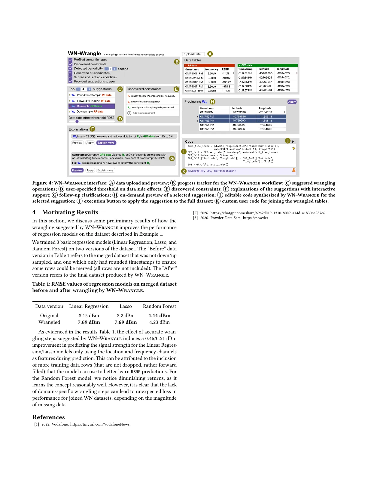
WN– W rangle : Wireless Netw ork Data W rangling Assistant Anirudh Kamath University of Utah USA anirudh.kamath@utah.edu Dustin Maas University of Utah USA dmaas@cs.utah.edu Jacobus V an der Merwe University of Utah USA kobus@cs.utah.edu Anna Fariha University of Utah USA afariha@cs.utah.edu Abstract Data wrangling continues to be the most time-consuming task in the data science pipeline and wireless network data is no exception. Prior approaches for automatic or assisted data-wrangling primar- ily target unordered, single-table data. However , unlike traditional datasets where rows in a table are unordered and assume d to be independent of each other , wireless network datasets are often col- lected across multiple measurement devices, producing multiple , temporally ordered tables that must b e integrated for obtaining the complete dataset. For instance, to create a dataset of the signal qual- ity of 5G cell to wers within a geographic region, GPS data collected by cellphones must be joined with radio-frequency measurements of the corresponding cell to wers. How ever , the join key timestamp typically exhibits mismatched sampling perio ds, causing a misalign- ment . Data-wrangling techniques for generic time-series datasets also fail here, since they lack knowledge of domain-sp ecic data semantics—often dened by network protocols and system con- gurations. T o aid in wrangling wireless network datasets, we demonstrate WN– Wrangle , an interactive wrangling assistant — tailored to the wireless network domain—that suggests the top-k next-best wrangling operations, along with rich, domain-specic explanations . Under the hood, WN– W rangle enforces temporal- constraints- and a wireless-network-semantics-aware mechanism to score and rank an extended set of wrangling operators to improve the data quality . W e demonstrate how WN–W rangle identies elusive data-quality issues specic to the wireless network domain and suggests accurate wrangling steps over datasets obtained from the widely used PO WDER city-scale wireless testbed. Link to demo video: https://users.cs.utah.edu/~afariha/wnwrangle.mp4 1 Introduction The fth generation (5G) of mobile networks is expected to serve nearly 3 billion users worldwide by 2026, with over 65% of xed wireless access connections projected to be provided via 5G by 2025 [ 9 ]. Supporting this scale demands intelligent service monitor- ing, provisioning, and network planning, all of which increasingly rely on data-driven AI/ML techniques. For instance, V odafone re- ported reducing data-ingestion latency from 36 hours to 25 minutes by leveraging insights from 70 petabytes of user-collected data [ 1 ]. Howev er , a critical prerequisite for learning from such data is mak- ing it analysis-ready , which in practice requires extensive and r ou- tine data wrangling of large-scale wireless network (WN) datasets. Data wrangling, in general, is often a te dious and time-consuming process. Data scientists reportedly sp end up to 60% of their time on tasks such as cleaning, imputing, transforming, and organizing data [ 7 ]. This has motivated the development of assistant tools for data wrangling (D W), such as Co W rangler [ 7 ] and W rangler [ 12 ], which can suggest relevant operations to expe dite the D W process. Howev er , such general-purpose D W assistants [ 7 , 17 ] fall short when applied to WN datasets for several reasons. First , they as- sume that rows within a dataset are unor dered and unrelated, often suggesting incorrect imputation or even dropping r ows with miss- ing values. For instance, Co W rangler’s [ 7 ] imputation suggestions are limite d to constant, mean, mo de, and me dian. WN datasets, howev er , are inherently temporal, with measurements recorded sequentially over time and often at xed sampling rates. Naïv ely applying a mean imputation can distort p eriodic signals; instead imputations must be done using appropriate forward or backward lling. Second , generic D W tools typically op erate on a single table, which fails when multiple tables must be joined via numer- ical join keys that are misaligne d due to dierent periodicity or measurement units. For instance, Auto-Suggest [ 17 ] fails to join over numerical keys with mismatched units (e.g., miles vs. kilo- meters). Third , existing D W assistants are domain-agnostic and ignore crucial semantics of WN data. For instance, logarithmic units such as decibel-milliwatts must b e converted to linear units b efore aggregation. W e proceed to highlight these issues in Example 1. Example 1. Naomi is collecting data to train an intelligent network conguration management system (Figure 1). This system requires per-second, complete radio frequency (RF) measurements across all fre- quency channels, with corresponding GPS co ordinates. She uses two de- vices for data collection: an RF measurement device that records data in the format 1 as shown in A , and a smartphone that records data in the format as shown in B . Her goal is to generate a dataset in the schema (shown in D ) by joining A and B over the join key timestamp . Howev er , while trying to join A and B , Naomi observes that the measurements are logged at dierent temporal granularities: A con- tains multiple entries within a se cond while B has missing entries for some seconds. Furthermore, there is no exact match between the timestamp attributes of the two tables and Naomi must temporally align them. Existing tools like Co W rangler [ 7 ] overlooks Naomi’s goal of joining A and B , and exacerbates the situation by making incorrect suggestions: (1) Dropping the row 𝑎 7 from A due to the missing RSRP , which results in losing the only entry for the corresponding timestamp and frequency . (2) Imputing a 7 [ RSRP ] with the arithmetic mean of RSRP , despite the unit for RSRP being logarithmic (decibel-milliwatts). T o join A and B , Naomi must ensure that (1) each frequency channel has exactly one RSRP reading p er second, as in A w ; (2) exactly one geo-location entry exists p er second in the GPS data, as in B w ; and (3) the values in timestamp in A & B match exactly . T o achieve this, the following wrangling steps are essential: 1 RSRP (Reference Signal Received Power) measures the power of the reference signal received by a device from a cell tower , typically expr essed in dBm, a logarithmic unit. 1 VLDB ’26 Demos, Boston, USA, Anirudh Kamath, Dustin Maas, Jacobus V an der Merwe, and Anna Fariha A B Radio Fr equency Meas urement Sample of t he raw datasets collected by Naomi GPS Locati on Data iss ues preve nting joi n of the raw da tase ts Wrangle d Radio Frequency Measurement Wrangle d GPS Location D Complete Datas et : Radio Fre quency measur ements w ith GPS locati ons for each f requency channel per se cond A W B W ⋈ = timestamp frequency RSRP 1:17:51.071 3.56e9 - 111.78 a 1 1:17:51.255 3.58e9 - 101.92 a 2 1:17:51.371 3.56e9 - 105.22 a 3 1:17:51.471 3.56e9 - 95.63 a 4 1:17:52.571 3.56e9 - 114.27 a 5 1:17:52.378 3.58e9 - 96.66 a 6 1:17:53.662 3.56e9 a 7 1:17:53.445 3.58e9 - 98.00 a 8 timestamp latitude longitude 1:17:51 40.769560 - 111.846113 b 1 1:17:54 40.769625 - 111.846112 b 2 1:17:55 40.769547 - 111.846113 b 3 timestamp frequency RSRP 1:17:51 3.56e9 - 99.93 a 1, a 3, a 4 1:17:51 3.58e9 - 101.92 a 2 1:17:52 3.56e9 - 114.27 a 5 1:17:52 3.58e9 - 96.66 a 6 1:17:53 3.56e9 - 114.27 a 7 1:17:53 3.58e9 - 98.00 a 8 ... ... ... timestamp latitude longitude 1:17:51 40.769560 - 111.846113 b 1 1:17:52 40.769560 - 111.846113 b 4 1:17:53 40.769560 - 111.846113 b 5 1:17:54 40.769625 - 111.846112 b 2 1:17:55 40.769547 - 111.846113 b 3 ... ... ... timestamp frequency RSRP latitude longitude 1:17:51 3.56e9 - 99.93 40.769560 - 111.846113 a 1, a 3, a 4 ⋈ b 1 1:17:51 3.58e9 - 101.92 40.769560 - 111.846113 a 2 ⋈ b 1 1:17:52 3.56e9 - 114.27 40.769560 - 111.846113 a 5 ⋈ b 4 1:17:52 3.58e9 - 96.66 40.769560 - 111.846113 a 6 ⋈ b 4 1:17:53 3.56e9 - 114.27 40.769560 - 111.846113 a 7 ⋈ b 5 1:17:53 3.58e9 - 98.00 40.769560 - 111.846113 a 8 ⋈ b 5 ... ... ... ... ... ... Three measurements within a second for the same frequency Missing value: imputation needs domain knowledge No exact match between timestamps Data missing at 1:17:52 & 1:17:53 A W B W Figure 1: A : RF measurement data sample, B : GPS data sample, A w & B w : desired wrangled datasets, D : desired complete dataset. Step 1 : Forward-ll the missing RSRP in a 7 using the value from a 5 , but not a 6 since the frequency channels are dierent. Step 2: (a) Merge rows a 1 , a 3 , and a 4 using techniques appropriate for logarithmic units—which ensures a per-second periodicity in A w —and (b) round down timestamps to the nearest second. Step 3: (a) Insert two empty rows between b 1 and b 2 to ll the miss- ing seconds and achieve a p er-second periodicity in B w , followed by (b) forward-lling location values in the newly inserted rows, because smartphones susp end GPS logging while stationar y to conserve power . Naomi had to spend 20 minutes writing and validating the mun- dane code snippet below—a disproportionate time cost despite her domain expertise—to obtain the desired dataset D = Aw ⊲ ⊳ Bw . # ( S t e p 1 ) F o r w a r d - f i l l R S R P p e r f r e q u e n c y A [ " R S R P " ] = A . g r o u p b y ( " f r e q u e n c y " ) [ " R S R P " ] . f f i l l ( ) # ( S t e p 2 ) P e r - s e c o n d l o g - a w a r e R F a g g r e g a t i o n A [ " s e c " ] = A [ " t i m e s t a m p " ] . d t . f l o o r ( " S " ) A [ " R S R P _ l i n " ] = 1 0 * * ( A [ " R S R P " ] / 1 0 ) A = A . g r o u p b y ( [ " s e c " , " f r e q u e n c y " ] ) . a g g ( { " R S R P _ l i n " : " m e a n " } ) A [ " R S R P " ] = 1 0 * A [ " R S R P _ l i n " ] . a p p l y ( l o g 1 0 ) A . d r o p ( c o l u m n s = " R S R P _ l i n " , i n p l a c e = T r u e ) # ( S t e p 3 ) P e r - s e c o n d G P S f o r w a r d - f i l l B = B . s e t _ i n d e x ( " t i m e s t a m p " ) . a s f r e q ( " 1 S " ) . f f i l l ( ) . r e s e t _ i n d e x ( ) A wrangling assistant for wireless network data . Example 1 demon- strates several wrangling operations that are specic to WN domain and are typically overlooked by generic wrangling assistants. This observation motivates the need for a specialized WN wrangling assistant that can proactively suggest domain-relevant wrangling operations. Such an assistant must satisfy the following require- ments: (i) respect temporal constraints, such as ensuring perio dicity and completeness (Step 1, Step 2 (a), & Step 3); (ii) support auto- matic alignment across tables through downsampling (Step 2 (a)), upsampling (Step 3 (a)), and homogenization (casting timestamp to the nearest second in Step 2 (b)); (iii) exploit inter-row r elation- ships, including appropriate imputation strategies (forward-lling in Step 1 and Step 3 ( b)); and (iv) pr eserve domain-specic semantic correctness, such as using imputation methods suitable for logarith- mic units (Step 2 (a)). Finally , to encourage broad adoption, a WN wrangling assistant should additionally provide (v ) rich explana- tions for its suggested operations; and (vi) interactive controls that allow users to inspect, customize, and guide the wrangling process. T emporal re-alignment is common across domains. . Datasets contain- ing temporal columns (i.e., containing timestamped measurements) inadvertently require temp oral r e-alignment to make them joinable. This is explicitly mentioned in multiple papers describing datasets in the domains of climate science [ 15 ], energy consumption [ 16 ], satellite networks [14], and more. W rangling WN data does not mean only temporal re-alignment. In WN data, there are multiple levels of abstraction that envelope the semantic meaning of columns. For example, frequency channels (often in the unit Mega-Hertz (MHz)) are represented as channel numbers (terme d EARFCN/ARFCN 2 ), which are 3GPP standardized representations for 4G/5G channels [ 5 ]. Due to commercial mea- suring e quipment often measuring channels in MHz, combining measurement data with protocol level datasets requires transfor- mation from MHz to EARFCN/ARFCN. While Example 1 demonstrates wrangling operations that are cen- tered around timestamp re-alignment of wireless measurements, other entities (e .g., wireless channel repr esentations) also require unit and format re-alignment, which we highlight in the example below . Example 2. Naomi now wishes to augment the RF measurements ( A in Figure 1) with details about the 4G/5G cells in the area that were transmitting on these channels (Figure 2). For this, she pro- cures an older dataset measured using a cellular modem device. This dataset contains the scanned cell towers in the form . In this scenario, Naomi wishes to join the two datasets by frequency and channel_number respectively , as they both contain the detected frequency that the cell tower trans- mitted on– however , channel numbers are represented in EARFCN 3 , whereas frequency values are represented in Megahertz (MHz). These are two units for the same entity , but she ne eds to map channel num- bers to downlink frequency values in MHz using a translation table dened by a standard do cument (3GPP TS 36.101 [ 5 ]), where each channel number has dierent coecients in the translation formula. 2 (E)ARFCN stands for (E-U TRA) Absolute Radio Frequency Channel Number 3 EARFCN stands for E-U TRA Absolute Radio Frequency Channel Numb er , an identier for the center frequency of wireless transmissions by a radio device. 2 WN– Wrangle : Wireless Network Data Wrangling Assistant VLDB ’26 Demos, Boston, USA, A C Radio Freq uency Measur ement Sample o f the r aw datasets Discovered Cell Details Wrangle d Serving Ce ll Det ails D Complete Dataset : Radio Fr equency measurements with discovered Cell ID and PL MN details for each frequency channel C W ⋈ = timestamp frequency RSRP 1:17:51.071 3.56e9 - 111.78 a 1 1:17:51.255 3.58e9 - 101.92 a 2 1:17:51.371 3.56e9 - 105.22 a 3 1:17:51.471 3.56e9 - 95.63 a 4 1:17:52.371 3.56e9 - 114.27 a 5 1:17:52.378 3.58e9 - 96.66 a 6 1:17:53.362 3.56e9 a 7 ... ... ... channel PLMN cell ID 55340 315010 82ABC c 1 55540 315010 2ABAB c 2 ... ... ... channel PLMN cell ID 3.56e9 315010 82ABC c 1 3.58e9 315010 2ABAB c 2 ... ... ... timestamp frequency RSRP PLMN Cell ID 1:17:51.071 3.56e9 - 111.78 315010 82ABC a 1 ⋈ c 1 1:17:51.255 3.58e9 - 101.92 315010 2ABAB a 2 ⋈ b 2 1:17:51.371 3.56e9 - 105.22 315010 82ABC a 3 ⋈ c 1 1:17:51.471 3.56e9 - 95.63 315010 82ABC a 4 ⋈ c 1 1:17:52.371 3.56e9 - 114.27 315010 82ABC a 5 ⋈ c 1 1:17:52.378 3.58e9 - 96.66 315010 2ABAB a 6 ⋈ c 2 1:17:53.362 3.56e9 315010 82ABC a 7 ⋈ c 1 ... ... ... ... ... ... Different channel representat ions for the same ch annels! A C W Figure 2: A : RF measurement data sample, C : Discovered cells data sample, c w : desired wrangled discovered cells dataset (with channel attribute converted to MHz), D : desired complete dataset. For this, she must know each channel number that is represented in the RF measurements table, translate them separately , and then join the tables. This also extends to other WN entities that can be repr esented in dierent ways. For example global cell identiers can be represented in hexadecimal or in de cimal, requiring conversion from unit to another . W e demonstrate WN– Wrangle , an interactive W ireless N et- work data- W rangl ing assistant that suggests top-k relevant wran- gling operations in a multi-table setting, tailored for WN datasets, satisfying the above six requirements. The key idea behind WN– Wrangle is temporal-constraint -aware scoring of WN-sp ecic wran- gling operations, which builds on the notion of temporal functional dependencies [6] to identify periodicity violations in the data. Related work . Prior works in the databases community [ 7 , 12 ] mainly target unordered relational datasets and thus fail on WN datasets, which are temporal in nature. T ools for cleaning temp oral data us- ing temporal integrity constraints [ 6 ] assume that domain-specic rules can be discovered from the data itself, which does not hold for the WN domain, where rules are often dictated by network pro- tocols or system congurations. Recent works on time-series data wrangling [ 13 ] are domain-agnostic and fail to provide alignment- related wrangling suggestions such as upsampling, downsampling, or homogenizing (as shown in Example 1). While wrangling code generation systems [ 11 ] and foundation models have achieved par- tial success due to their ability to understand data semantics, they still struggle with complex tasks such as joining multiple incomplete datasets with misaligne d join keys. For instance, when asked to join the datasets A and B while ensuring one record per second, Chat- GPT made several mistakes, including incorrect RSRP imputation, incorrect frequency aggregation, and failing to up/downsample [ 2 ]. Commercial tools for time-series data [ 8 ] primarily target enterprise data sources and require extensiv e manual conguration. Demonstration. In our demonstration, participants will observe how WN– W rangle identies temporal inconsistencies in two real- world datasets collected using the PO WDER [ 10 ] city-scale wireless testbed, and suggests accurate wrangling steps in an explainable and interactive manner . W e will showcase how a user can customize the suggestions in two WN data analysis scenarios—one to improve the readability of radio-frequency readings on a map interface, and the other to improv e an ML model’s performance on the collected data. W e provide an overview of WN–W rangle ’s inner working in Section 2, and a walkthrough of the demonstration scenario based on Example 1 in Section 3. 2 System overview WN– W rangle targets multiple WN tables that share a conte xt that allows their joint use via joins While we fo cus on the temporal context in this WN– W rangle also supports joining over frequency channels, and spatial coordinates, and cell tow er identities by lever- aging the corresponding alignment semantics. Challenges. W e identify the following key challenges towards build- ing WN– W rangle : (C1) How to model WN goal-oriented specic constraints and detect their violations in the data? (C2) Which WN-specic wrangling operations should be considered as candi- dates for repairing the constraint violations? (C3) How to quantify the eectiveness of candidate wrangling operations—i.e., score and rank them—to enable accurate top- 𝑘 suggestions automatically? (C4) How to generate domain-aware explanations for the sugges- tions, while allowing users to (optionally) guide the wrangling process interactively ? Overview . T o addr ess these challenges, WN– W rangle comprises ve components: (§2.1) a semantic proler that proles the data attributes; (§2.2) a constraint discov ery module that discovers WN- specic constraints; (§2.3) a Domain Specic Language (DSL) tailored towards WN data; (§2.4) a scoring method that evaluates eective- ness of candidate wrangling operations; and (§2.5) an explanation module that generates explanations for the suggestions. The system architecture worklow is described in Figure 3. 2.1 Semantic profiler . WN– W rangle must understand the data characteristics to mo del WN-specic constraints ( C1 ), support scor- ing of wrangling operations ( C3 ), and provide explanations ( C4 ). T o this end, WN– Wrangle emplo ys a semantic proler that analyzes 3 VLDB ’26 Demos, Boston, USA, Anirudh Kamath, Dustin Maas, Jacobus V an der Merwe, and Anna Fariha Semantic profiler Constraint disc. User interaction time freq RSRP time chan PLMN CellID 2025-1 0-22 19:33:32.371 2025-1 0-22 19:33:32.571 2025-1 0-22 19:33:32.6 77 2.00e9 3.56e9 3.64e9 -111. 63 -111. 63 -111. 63 2023- 10-22 12:12:24 2023- 10-22 12:12:24 2023- 10-22 12:12:24 56140 55340 56140 time(A) → msec → timestamp→ groupby time(B) → sec → timestamp → groupby freq(A) → MHz → numerical → groupby chan(B) → EARFCN → numerical → groupby RSRP(A) → dBm → numerical → aggregate ... T able A T able B [Δ(A), freq(A) → RSRP(A)] [chan(B) → PLMN(B), CellID(B)] 311480 311480 315010 Join by timestamp or channel? Generated constraints Join by channel! Also, ensure 1 second granularity Score and suggest Explanations Use violations detected as basis to explain Ranked list based on constraints and types: 1. Convert chan(B) to MHz 2. Convert time(A) to sec 3. Aggregate RSRP(A) groupby freq, time 4. ... 2CCCABC B2CFD 2CCCABC Generated semantic profiles Apply/ skip suggestion Figure 3: System architecture of WN– Wrangle . After data upload, semantic proling (Section 2.1) generate feature proles per column (units, type, aggregation/imputation role), the constraint discovery module (Section 2.2) uses these proles to identify joinable columns and devises constraints to enforce to enhance the join, after which the scoring and suggestion of wrangling op erations (Section 2.4) on the basis of constraints and feature proles, and explanation synthesis (Section 2.5) is done in a human-in-the-loop workow , where the user can apply suggestions or skip them over . each data attribute over a small sample to infer the following key aspects about them: • its data type (e.g., numerical, categorical, or dinal); • its semantic type, measurement unit, and scale (e.g., RSRP mea- sures signal power in dBm , a logarithmic scale); • semantically correct aggregation strategies ( e.g., using Frequency as a grouping column when aggregating RSRP); T o obtain the above information, WN– W rangle queries a general- purpose LLM (GPT -5.2). These queries are issued carefully using crafted prompts to the LLM to ( Q1 ) the column unit (e.g., dBm, or MHz), ( Q2 ) gather the broad typ e (e.g., numerical or categori- cal) and ( Q3 ) whether this column is “gr ouping” or “aggregating” (aggregating/imputation r oles). Below is the query template WN– W rangle crafts to assess the measurement units of values in the column ( Q1 ). WN–W rangle ’s measurement units are pre-dened for wireless types. Howev er , our demo also allows participants to congure their o wn units as keywords to ensure generalization when using datasets from other domains. Question : Y ou are an expert wireless data proler . I have a column in a pandas dataframe named chan. It has a minimum value of 800.0, max value of 68661.0, and 18 unique values. Here are some sample values: . . . T ell me the unit of this column’s values- only choose from [’no unit’ , ’MHz’ , ’Hz’ , ’EARFCN’ , ’ dBm’ , ’dB’ , ’hexadecimal’ , ’decimal’ , ’seconds’, ’milliseconds’]. For example, a test score has no unit, so answer "no unit" . Howev er , a temperature has a unit "celsius" . Answer only either [’no unit’ , ’MHz’, ’Hz’ , ’EARFCN’ , ’dBm’ , ’dB’ , ’hexadecimal’ , ’decimal’], and nothing else. Answer : EARFCN After this, WN– Wrangle assesses the br oad data type ( Q2 ) for each unit via the query template shown b elow . T o do this, WN– Wrangle uses the result of the previous query , and asks the LLM if data fr om a column labeled with a certain unit should be numerical, categorical, or ordinal. For example, the RSRP column is proled with a unit of dBm , so it is “numerical” and should b e treated as such. Question : Y ou are an expert wireless data proler . I have a data in a column named RSRP with the unit of dBm. Here is a sample of that data: . . . T ell me if data with this unit’s values are timestamp, cate- gorical, numerical, or ordinal. For example, temp erature ’s unit is celsius, so it is a "num- ber" , even if some values are string values in it (to repre- sent missing values). For example, even though a bank account ID has no unit, it is "categorical" b ecause the records can b e grouped by bank account ID. For example, even though a score ranging from 1 to 5 is a number , because it has no unit, it is "ordinal" . Answer only either "timestamp" , " categorical" , "numerical" , or "ordinal" , and nothing else. Answer : numerical Finally , WN– Wrangle gathers information about per-column ag- gregation and imputation roles ( Q3 ). The LLM is asked if the context of the attribute’s values warrants its usage as a “grouping” attribute (e .g., if it is categorical), or if it is an “aggregating” attribute (e .g., it is a numerical value changing over time). This is crucial, because ev en though some columns may be proled as numerical, it may well b e a column that must b e use d to group together rows in aggregations– for example, the freq column in T able A (Figure 3) is numerical, but it is denitely a grouping attribute when aggr egating RSRP values to get a per-second granularity . 4 WN– Wrangle : Wireless Network Data Wrangling Assistant VLDB ’26 Demos, Boston, USA, Question : Y ou are an expert wireless data proler . I have a column in a pandas dataframe name d chan, with other columns in the dataframe being [’ cellid’ , ’PLMN’]. It has a unit of EARFCN. Here are some sample values: . . . Y ou should de cide if this column goes in the ‘agg()‘ part ("aggregating"), or if this column goes in the ‘groupby‘ part ("grouping") of an aggregation quer y in pandas. For example, in a dataframe with columns , date and product_id are as- signed "grouping" , and units_sold "aggregating" . Answer only either "aggregating" or "grouping" and nothing else. Answer : grouping Using the information gathered from the LLM responses, WN– Wrangle synthesizes the following based on the attribute ’s prole: (1) semantic-type- and domain-aware imputation strategies (e.g., forward-lling GPS locations, as columns with data type decimal degrees unit is imputed by forward lling); and (2) semantic-type- and domain-aware aggregation strategies (e .g., converting to linear scale b efore averaging logarithmic values, as dBm unit values require this special technique for accurate aggregation); and (3) domain-aware type casting between attributes (e.g., chan attribute in T able B in Figure 3 should be conv erted to MHz, the unit of freq channel). Remark: Our demo only supp orts type casting (item 3 above) b e- tween pre-congured wireless data types ( e.g., EARFCN to MHz), as this requires explicit pr ogramming of a casting function in the DSL (Section 2.3). Adding more type casting functions to the DSL is trivial per unit pair . 2.2 Constraint discovery mo dule . T o address C1 , this module models WN-specic data constraints (e.g., temporal constraints requiring per-second measurements) and detects their violations in the data. Since enforcing these constraints ensures temp oral and informational completeness, they provide guidance for sug- gesting wrangling operations that reduce constraint violations. T o model temporal constraints, we use the established notion of tem- poral functional dependencies (TFDs) [ 6 ]. For example, 𝑇 𝐹 𝐷 1 = [ Δ , frequency ] → RSRP denotes the temporal constraint of having “ ex- actly one RSRP record per second per frequency channel” , where Δ = 1s denotes a xed periodicity in timestamp . User interaction. The constraint discovery module rst conrms with the user which columns to use to join the tables. It does so by presenting potential options based on similar units which can be converted (e.g., milliseconds to seconds), or transformed (e.g., EARFCN to MHz). For instance, in Figure 3, the user does not wish to join over timestamps, and instead, the constraint discovery module recognizes (from semantic proles) that EARFCN and MHz are units repr esenting transferable units that can be transformed to each other . Synthesizing constraints. Once the user conrms the joining columns, WN– W rangle synthesizes TFDs and associated parameters by leveraging semantic data proles—which pr ovides derived knowl- edge such as “within a second granularity in the RF measurements table, it is required that each frequency (grouping categorical at- tribute) requires non-empty RSRP ” (to ensure no loss of temp oral granularity). Specically , WN– Wrangle identies a common pe- riodicity Δ that can be achieved across the data tables without impacting too many tuples (minimizing side-eects) and conrms this with the user . While TFD discovery [ 6 ] is fully automated, WN– W rangle supports optional user input to validate Δ and to specify custom TFDs, thereby addressing C4 . Detecting violating tuples. WN– Wrangle ags tuples within the inferred periodicity that violate TFDs. E.g., in Figure 1, a 1 , a 3 , and a 4 violate 𝑇 𝐹 𝐷 1 due to multiple RSRP , while a 7 due to missing RSRP . 2.3 DSL for WN . T o address C2 , we need a domain-specic lan- guage that includes common operators used in WN data analysis. In this demo, we include frequently used operators identied through analyzing scripts from members of the PO WDER [10] team. (1) Upsample : Achieves the giv en temporal granularity by insert- ing new ro ws and lling in empty cells (Step 3 of Example 1). T o do this, the semantic prole is used to choose between the following options: (a) forward lling, (b) backward lling, (c) interpolation, using a combination of the grouping attributes found by the semantic proler to group and impute newly cre- ated rows . A [ " R S R P " ] = A . g r o u p b y ( " f r e q u e n c y " ) [ " R S R P " ] . f f i l l ( ) (2) Downsample : Achiev es the given temporal granularity by ag- gregating existing rows (Step 2 of Example 1). T o do this, a combination of the grouping attributes found by the semantic proler is used to group and aggregate using functions (e.g., logarithmic mean) from a pre-dened list of aggregation func- tions. An example of a downsample call would translate to the following pandas co de: d f . g r o u p b y ( [ " t i m e s t a m p " , " f r e q u e n c y " ] ) . a g g ( { " t h r o u g h p u t " : " m e a n " } ) (3) Impute : Imputes a cell using the given technique such as forward-ll or backward-ll (Step 1 of Example 1), using a combination of the grouping attributes found by the seman- tic proler to group and impute. Translates to a pandas for- ward/backward ll operation. Example: d f [ " l a t i t u d e " ] = d f [ " l a t i t u d e " ] . f f i l l ( ) (4) Rounds : Rounds dierently scaled units to the nearest homo- geneous unit (e.g., rounding millisecond timestamps to se conds, based on the specied p eriodicity (Step 2 of Example 1)). Trans- lates to a pandas code that is crafted based on the semantic type of the column. For example, for a time column: d f [ " t i m e s t a m p " ] = d f [ " t i m e s t a m p " ] . d t . f l o o r ( " S " ) (5) Cast : Cast from one unit to another unit to facilitate joins over columns with dierent repr esentations of the same entity (Example 2). As discussed previously , the current version of WN– W rangle allows for type casting for WN specic types. Some examples: • EARFCN ← → MHz (for frequency channels) • Integer ← → Hexadecimal (for cell IDs) • Object − → Datetime (for timestamp columns) 5 VLDB ’26 Demos, Boston, USA, Anirudh Kamath, Dustin Maas, Jacobus V an der Merwe, and Anna Fariha • Object − → Float (for numerical columns) (6) Drop row : Drops rows based on the given conditions. For in- stance, drop rows that are not numerical in a column that is proled to be numerical. Remark: The above DSL is spe cic for handling WN-data issues and should be treated as insucient to r esolve generic issues such as formatting inconsistencies (e .g., date format), for which a generic D W tool [7, 13, 17] can be use d. 2.4 Scoring method . WN– Wrangle generates a set of candidate operations by parameterizing the DSL operators with appropriate parameters. During this step, WN– W rangle prunes semantically invalid candidates, i.e., those that violate WN-sp ecic semantics, such as using an arithmetic mean as an imputation technique for RSRP by quer ying an LLM to verify which of the generated DSL instances are accurate. This automates away the ltering a domain expert would encounter if all options were provided to only present semantically valid wrangling operations. An example when quer y- ing GPT -5.2 is pr ovided below: Question : Y ou are an expert wireless data proler . I have a column in a pandas dataframe named RSRP. It has a unit of dBm. Here are some sample values: . . . Y ou should de cide what aggregation method to use to com- bine multiple values into one data p oint. Y our choices are: [’mean’, ’sum’ , ’mode’ , ’median’, ’log_mean’]. Their descriptions are: [’arithmetic mean’ , ’sum’ , ’most fre- quent value’ , ’50th percentile value’ , ’convert to linear do- main, do arithmetic mean, convert back to log domain’]. Answer only one of [’mean’ , ’sum’ , ’mode’ , ’median’ , ’log_mean’] and nothing else. Answer : log_mean While this reduces the search space, a key challenge ( C3 ) remains: determining which of these candidates should be suggested to the user . T o this end, WN– W rangle employs an ecient scoring method that estimates the expe cted improvement in data quality— i.e., the reduction in constraint violations—if a candidate wrangling operation were applied to the data. Given a dataset 𝐷 , discovered constraints or rules 𝑅 , semantic proles 𝑆 , candidate wrangling operations 𝑊 , and a violation func- tion 𝑉 ( 𝐷 , 𝑅 ) that computes the degree of violation by 𝐷 w .r .t 𝑅 , the scoring method applies each 𝑤 ∈ 𝑊 to a small sample of the data 𝐷 ′ to obtain 𝐷 ′ 𝑤 , where the sampling technique used is awar e of the WN-specic semantics. This enables WN– Wrangle to eciently estimate the e xpecte d data-quality impr ovement when 𝑤 is applied over 𝐷 as 𝑉 ( 𝐷 ′ , 𝑅 ) − 𝑉 ( 𝐷 ′ 𝑤 , 𝑅 ) . While minimizing constraint vio- lations is the primary objective, WN– W rangle also accounts for data side eects by ensuring that each of the 𝑘 suggested wrangling operations satisfy a predened data-side-eect budget ( e.g., at most 𝑝 % cells/rows of the data can be modied). 2.5 Explanation module . Finally , the explanation module com- bines the information from the semantic pr oler , constraints dis- covered and violations detected by the constraint discovery module, and the estimated reduction in violation obtained by the scoring method to generate a human-understandable, natural-language explanation for each of the suggested wrangling operations. 3 Demonstration W e will demonstrate WN–W rangle over real-world PO WDER datasets [ 3 ]. W e will guide users through eleven steps of Figure 4 impersonating Naomi over the dataset [4] of Example 1. Step A ○ (Data upload and preview ) . The user uploads two data les RF.csv and GPS.csv and previe ws the data. WN– W rangle displays the rst ve rows. The user can scr oll to see more. Step B ○ (W orkow progress tracker) . WN–W rangle semanti- cally proles the data attributes (§2.1); discovers temporal and other constraints and dete cts the p eriodicity parameter Δ (§2.2), which the user can rene if they wish to; generates 56 wrangling candidates, scores, and ranks them (§2.4) to generate the suggestions. Step C ○ (W rangling suggestions) . WN– W rangle suggests 4 operations: 𝑊 1 , 𝑊 2 , & 𝑊 4 for the RF data and 𝑊 3 for the GPS data. Step D ○ (Data side-ee ct) . Along with the suggestions, WN– Wrangle displays maximum data side-eect incurred (10% ro ws were impacted) by any of the suggestions. The user can adjust the side-eect threshold and WN– Wrangle ensures that each sug- gested operation satises the user-specied side-eect requirement. Step E ○ (Discovered constraints) . WN– W rangle lists the constraints (three in this case) that it used to compute the degree of violation for scoring the candidate wrangling op erations. For example, the constraint 𝑅 1 : “ exactly one RSRP record per second per frequency ” applies to the RF data. The user can add ne w constraints. Steps F ○ & G ○ (Explanation and interaction) . The user wants to understand the rationale behind the suggestion 𝑊 3 . WN– Wrangle provides an initial explanation—“ 𝑊 3 inserts 7% new rows, satisfying 𝑅 3 ”—along with options to Preview its impact, A pply 𝑊 3 to the full data, or request further Explanation . After sele cting “ Explain more , ” WN– W rangle oers a detaile d explanation describing missing readings across multiple se conds. Satised, the user chooses to Preview the impact of 𝑊 3 on the GPS data. Step H ○ (Preview suggestion impact) . WN– Wrangle pre- views the impact of 𝑊 3 on a small sample of the GPS data, highlight- ing ne wly inserted rows by “+” . Satised, the user clicks on “ Apply” . Steps I ○ & J ○ (A utomatically generated wrangling co de) . WN– W rangle inserts an editable code snippet for 𝑊 3 to the user notebook, and automatically executes it in Step J ○ . The user accepts the other three suggestions in a similar way (not shown). Step K ○ (Custom co de) . Finally , the user successfully joins the two (now wrangled) datasets as per Example 1. While WN– W rangle applies to any WN data scenario, it is espe- cially useful for experimental wireless testbe ds like PO WDER [ 10 ], where hundreds of users generate diverse datasets from 2 , 000 + yearly experiments, supporting advanced wireless applications. 6 WN– Wrangle : Wireless Network Data Wrangling Assistant VLDB ’26 Demos, Boston, USA, Dis c o v er ed c on str ain t s D e t ec t ed per i odi c i t y Pro led s em an ti c t ypes Gener a t ed 56 c andi da t es s ec ond S c or ed and r ank ed c andi da t es Pro v i ded s u ggesti on s t o u s er W 1 W 2 R ound timestamp in RF da t a W 3 F orw ar d ll R S RP in RF da t a W 4 D o wn s ample RF da t a Ups ample GP S da t a T op s u ggesti on s D a ta s i de - e f f ec t thr eshold ( 10 % ) R 2 no r ec or d w i th mis s ing R S RP R 1 e x ac tly one R S RP per s ec ond per fr equ enc y R 3 e x ac tly one la ti t u de , longi t u de per s ec ond Dis c o v er ed c on str ain t s A dd ne w c on s tr a in t E xplan a ti on s Apply Apply Apply Pr e v i e w E x pla in m or e Pr e v i e w E xplain mor e F i x: s u ggest s adding 7 8 ne w ro w s t o s a tisf y the c on str ain t Symp t om s : C urr en tly , v i ola t es a s 7 % o f s ec onds ar e mis s ing w i th no la ti t u de / longi t u de r ec or ds . F or e x ample , no r ec or d a t timestamp 1 : 1 7 : 5 2 P M. GP S da t a R 3 R 3 W 3 in s er t s 7 8 ( 7% ) ne w ro w s and r edu c es v i ola ti on o f in from 7% t o 0 % . GP S da t a W 3 R 3 D a ta ta b les t i m e s t a m p lon g i t u de la t i t u de 4 0 . 7 6 959 0 - 1 1 1 . 846 1 1 3 - 1 1 1 . 846 1 1 2 - 1 1 1 . 846 1 1 3 - 1 1 1 . 846 1 1 3 - 1 1 1 . 846 1 1 3 4 0 . 7 6 9 625 4 0 . 7 6 954 7 4 0 . 7 6 95 1 1 4 0 . 7 6 95 0 1 0 1 : 1 7 : 56 P M 0 1 : 1 7 : 5 7 P M 0 1 : 1 7 : 54 P M 0 1 : 1 7 : 5 1 P M 0 1 : 1 7 : 5 5 P M GP S da t a t i m e s t a m p R S R P f r e q u enc y 0 1 : 1 7 : 5 1 . 25 5 P M 0 1 : 1 7 : 5 1 . 3 7 1 P M 0 1 : 1 7 : 5 1 . 4 7 1 P M 0 1 : 1 7 : 5 2 . 5 7 1 P M 0 1 : 1 7 : 5 1 . 0 7 1 P M 3 . 56 e 9 - 1 1 1 . 7 8 - 10 1 . 9 2 - 10 5 . 2 2 - 95 . 63 - 1 1 4 . 2 7 3 . 58 e 9 3 . 56 e 9 3 . 56 e 9 3 . 56 e 9 R F da t a C ode full_time_index = pd.date_range(start=GPS["timestamp"].iloc[0],  end=GPS["timestamp"].iloc[-1], freq=f'1S') GPS_full = GPS.set_index("timestamp").reindex(full_time_index) GPS_full.index.name = "timestamp" GPS_full[["latitude", "longitude"]] = GPS_full[["latitude", "longitude"]].ffill() GPS = GPS_full.reset_index() pd.merge(RF, GPS, on="timestamp") Pr e v i e w ing W 3 t i m e s t a m p lon g i t u de la t i t u de 0 1 : 1 7 : 5 2 P M 0 1 : 1 7 : 53 P M 0 1 : 1 7 : 54 P M 0 1 : 1 7 : 5 5 P M 0 1 : 1 7 : 5 1 P M 4 0 . 7 6 959 0 - 1 1 1 . 846 1 1 3 - 1 1 1 . 846 1 1 3 - 1 1 1 . 846 1 1 3 - 1 1 1 . 846 1 1 2 - 1 1 1 . 846 1 1 3 4 0 . 7 6 959 0 4 0 . 7 6 959 0 4 0 . 7 6 9 625 4 0 . 7 6 954 7 + + Upload D a ta C D E F G H I J K B A W N- W r an g le a wr angling a s s istan t f or w ir eles s ne tw ork da ta an aly s is 1 - + 4 - + Figure 4: WN– Wrangle interface: A ○ data upload and preview; B ○ progress tracker for the WN–W rangle workow; C ○ suggested wrangling operations; D ○ user-specied threshold on data side ee cts; E ○ discovered constraints; F ○ explanations of the suggestions with interactive support; G ○ follow-up clarications; H ○ on-demand preview of a selected suggestion; I ○ editable code synthesized by WN– W rangle for the selected suggestion; J ○ execution button to apply the suggestion to the full dataset; K ○ custom user code for joining the wrangled tables. 4 Motivating Results In this section, we discuss some preliminary results of how the wrangling suggested by WN– Wrangle impro ves the performance of regression models on the dataset described in Example 1. W e trained 3 basic regression models (Linear Regression, Lasso, and Random Forest) on two v ersions of the dataset. The “Before ” data version in Table 1 refers to the merged dataset that was not down/up sampled, and one which only had rounded timestamps to ensure some rows could be merged (all ro ws are not included). The “ After” version refers to the nal dataset produced by WN– W rangle . T able 1: RMSE values of regression mo dels on merged dataset before and after wrangling by WN– W rangle . Data version Linear Regression Lasso Random Forest Original 8 . 15 dBm 8 . 2 dBm 4.14 dBm W rangled 7.69 dBm 7.69 dBm 4 . 23 dBm As evidenced in the results T able 1, the ee ct of accurate wran- gling steps suggested by WN– W rangle induces a 0 . 46 / 0 . 51 dBm improvement in predicting the signal strength for the Linear Regres- sion/Lasso models only using the lo cation and frequency channels as features during prediction. This can b e attributed to the inclusion of more training data r ows (that are not dropped, rather forward lled) that the model can use to better learn RSRP predictions. For the Random Forest model, we notice diminishing returns, as it learns the concept reasonably well. However , it is clear that the lack of domain-specic wrangling steps can lead to unexpected loss in performance for joined WN datasets, dep ending on the magnitude of missing data. References [1] 2022. V odafone. https://tinyurl.com/V odafoneNews. [2] 2026. https://chatgpt.com/share/6962d019- 1310- 8009- a14d- a18306a987e6. [3] 2026. Powder Data Sets. https://p owderwireless.net/data. [4] 2026. RF and GPS Dataset. https://powderwireless.net/data#2026- cell- metrics. [5] 3GPP. 2025. Evolved Universal Terr estrial Radio Access (E-U TRA); User Equipment (UE) radio transmission and reception . T echnical Specication (TS) 36.101. 3rd Generation Partnership Project (3GPP). https://portal.3gpp.org/desktopmodules/ Specications/SpecicationDetails.aspx?specicationId=2411 V ersion 19.3.0. [6] Z. Abedjan, C. G. Akcora, M. Ouzzani, P. Papotti, and M. Stonebraker. 2015. T emporal rules discovery for web data cleaning. PVLDB 9, 4 (2015). [7] B. Chopra, A. Fariha, S. Gulwani, A. Z. Henley , D . Perelman, M. Raza, S. Shi, D . Simmons, and A. Tiwari. 2023. CoW rangler: Re commender System for Data- W rangling Scripts. In SIGMOD 2023 . [8] DataRobot. 2025. Time-aware data wrangling. https://shorturl.at/IdViw. [9] Ericsson. 2025. Ericsson Mobility Report. https://shorturl.at/kG4L3. [10] J. Breen et al. 2021. Powder: Platform for Open Wireless Data-driven Experimental Research. Computer Networks 197 (2021). [11] J. Huang, D . Guo, C. W ang, J. Gu, S. Lu, J. P . Inala, C. Y an, J. Gao , N. Duan, and M. R. Lyu. 2024. Contextualized Data-W rangling Code Generation in Computational Notebooks. In ASE . [12] S. Kandel, A. Paep cke, J. Hellerstein, and J. Heer . 2011. W rangler: interactive visual specication of data transformation scripts. In CHI . [13] L. Liu, S. Hasegawa, S. K. Sampat, M. Bahrami, W .-P . Chen, K. T oyota, T . Kato , T . Akazaki, A. Ura, and T . Asai. 2025. AutoDW- TS: A utomated Data W rangling for Time-Series Data. In CIKM . [14] Clemens Lottermoser , Simon Damm, and Stefan Schmid. 2026. Measur- ing W eather Eects and Link Quality Dynamics in LEO Satellite Networks. arXiv:2603.14008 [cs.NI] [15] William Morrison, Dana Looschelders, Jonnathan Céspe des, Bernie Claxton, Marc- Antoine Drouin, Jean-Charles Dupont, Aurélien Faucheux, Christopher C Holst, Simone Kotthaus, V aléry Masson, James Mcgregor , Jeremy Price, Matthias Zeeman, Sue Grimmond, and Andreas Christen. 2025. Harmonised boundar y layer wind prole dataset from six ground-based Doppler wind lidars in a transect across Paris, France. Earth System Science Data 17, 11 (2025), 6507–6529. doi:10. 5194/essd- 17- 6507- 2025 [16] Martin Pullinger , Jonathan Kilgour , DK Arvind, Heather Lovell, Johanna Moore, David Shipworth, Charles Sutton, Jan W ebb, and Niklas Berliner . 2021. The IDEAL household energy dataset, electricity , gas, contextual sensor data and sur vey data for 255 UK homes. Scientic Data 8, 1 (2021), 1–17. doi:10.1038/s41597- 021- 00921- y [17] C. Y an and Y . He . 2020. Auto-Suggest: Learning-to-Recommend Data Preparation Steps Using Data Science Notebooks. In SIGMOD 2020, online conference [Portland, OR, USA], June 14-19, 2020 . ACM, 1539–1554. doi:10.1145/3318464.3389738 7