Interpretable Physics Extraction from Data for Linear Dynamical Systems using Lie Generator Networks

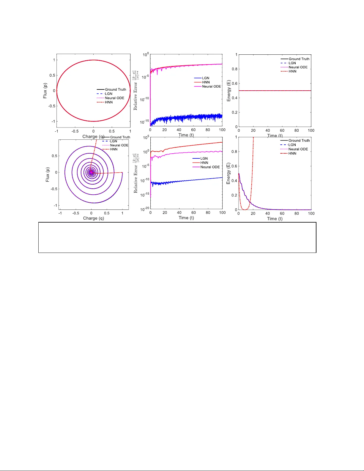
Interpretable Physics Extraction from Data for Linear Dynamical Systems using Lie Generator Network s Shafayeth Jamil, and Rehan Kapadia Department of El ectrical and Com puter Engineerin g University of Sou thern Californ ia sjamil@usc.edu, rkapadia@usc. edu Abstract When the system is linear, why should learning be nonlinear? Linear d ynamical systems, the analytical backbone of control theory , signal processing and circuit analysis, have exact closed- form solutions via the state transition matrix. Yet when system parameters must be inferred from data, recent neural approaches o ffer flexibility at the cost of physical guarantees: Neural ODEs provide flexible trajectory approximation but may violate physica l invariants, while energy- preserving architectures do not natively represent dissipation essential to real-world systems. We introduce Lie Generator Networks (LGN), whi ch learn a structured generator A and compute trajectories di rectly via matrix exponentiation. This shift from integra tion to exponentiation preserves structure by construction. By pa rameterizing A = S − D (skew-symmetric minus positive diagonal), stability and dissipation emerge from the underlying architecture and are not introduced during training via the loss function . LGN provid es a unified fram ework f or li near conservative, dissipative, and time-varying systems. On a 100-dimensional stable RLC ladder, standard derivative-based least-squares system identific ation can yield unstable eigenvalues. Th e unconstrained LGN yields stable but physica lly i ncorrect spectra, whereas LGN- SD recovers all 100 eigenvalue s with over two orders of m agnitude lower mean eigenvalue error than unconstrained alternatives. Critically, these eigenvalues reveal poles, natural frequencies, and damping ratios which are interpretable physics that black-box networks do not provide. Introduction Learning dynamical systems from data is fundamental to science and engine ering. Linear syst ems , described by  󰇗 󰇛  󰇜  󰇛 󰇜 󰇛󰇜 where matrix  󰇛 󰇜 is the system matrix, arise across domains, including circuit analysis, control theory, molecular dynamics, financial modeling, and linearization of nonlinear PDEs. When the generat or 󰇛 󰇜 can be recovered fro m trajectory data, its eigenvalues yield modal structure, stabili ty properties, characteristic timescales enabling not just prediction but interpretation and design. Classical system identification recovers  󰇛 󰇜 via least-squares regre ssion on estimated derivatives [1]. This is well -posed in low dimensions with clean data, but scales poorly because derivative estimation amplifies noi se, and unconstrained regression over n² pa rameters admits physically invalid solutions. Neural ODEs [2] elegantly parameterize continuous dynamics as  󰇗 󰇛󰇜    󰇛   󰇜 enabling learning from irregularly-sampled data. On the other hand energy-preserving neural networks such as HNN s [3], LNN s [4], and SympNet s [5] impose structure by learning energy functions and preserving phase-space volume. However, these neural models share fundamental limi tations. First, numerical integration accumulates error; struct ure preservation is approxim ate and degrades over long horizons. Second, energy-conserving methods in their standard form represent only conservative systems and dissipative extensions [9, 10] rely on numerical integration, inheriting its error a ccumulation. Third, the learned re presentations are opaque as a Neura l ODE p rovides no direct identification of underlying system physic s, such as poles, damping ratios, or natural fr equencies. Fourth, for linear systems, these methods solve a harder problem than necessary, which is approximating ẋ = Ax with a nonlinear    when the exact solution x(t) = exp(At)x₀ is available in c losed form. We introduce Lie Generator Networks (LGN), which learn the system m atrix A and evolve states via matrix exponentiation rather than numerical integration. For the Linea r time invariant (L TI ) case, x(t) = exp(At)x₀ is evaluate d directly. In the Linear time-varying (LTV) case, we employ the Magnus expansion [6] to handle non-commuting genera tors. This replaces derivative estimation and step-by-step integration with a structured generator-l earning problem. The generator matrix exponential pres erves th e underlying structure. For example, if w e constrain A to have certain properties such as eigenvalues with negative real parts, th e solution exp(A)x₀ inherits those properties exactly. LGN provides a unified framework for linear c onservative, dissipative, LTI and LTV systems. By parameterizing A = S – D , where S is skew-symmetric and D is positive diagonal, the S- D decomposition guara ntees all e igenvalues satisfy Re(λ) ≤ 0 and qua dratic energy dissipates monotonically. This gives us structure preservation to machine precision that is enforced by the architecture. For LTV systems, the Magnus truncation does not giv e us machine precision, but inherits  󰇛  󰇜 local error as shown by classical Magnus theory [7]. This gives us rigorous error bo unds. The S -D constraint also acts as implicit regular ization, enabling robust eigenvalue recovery even f rom noisy measurements. Essential ly, the learned system matrix, A directly reveals the physics of the underlying system, somethi ng other current machine syst em poles, natural frequencies, and damping ratios which are interpretable physics that bl ack-box methods do not offer. Method We study learning linear dynamical systems from trajectory observations. The systems under consideration here are based on data samples 󰇝 󰇛     󰇜󰇞   from an underlying system,  󰇗 󰇛  󰇜   󰇛  󰇜  󰇛  󰇜  The goal is to recover a generator 󰇛  󰇜 such that the learned dynamics mat ch the data while preserving kno wn physical structure (e.g., conservation, stability, dissipation). Rather than learning a gen eric nonlinear vector field and numerically integ rating it, Li e Generator N etworks (LGN) learn the gene rator directly and evolve states through matrix exponentiation, yielding closed-form flow maps for linear systems. LGN for LTI systems For the linear time-invariant (LTI) case 󰇛 󰇜   , trajectories admit the closed form  󰇛 󰇜  󰇛  󰇜    LGN learns a structured parameterization   and predicts   󰇛  󰇜  󰇛    󰇜    This approach can be described as le arn  , then exponentiate, and avoids deri vative estimation and numerical integration drift. Moreover, by constraining   to a physically valid class, then 󰇛   󰇜 inherits the corresponding structure by c onstruction. LGN for LTV systems For linear time-varying (LTV) dynamics, the solution can be wr itten as a single exponential  󰇛 󰇜  󰇛󰇛 󰇜󰇜    where 󰇛 󰇜 is given by the Magnus expansion 󰇛 󰇜   󰇛     󰇜              󰇟󰇛      󰇜 󰇛  󰇜󰇠       󰇟   󰇠      The first term captures the accumulated g enerator, while higher-o rder terms correct for non- commutativity when 󰇟󰇛  󰇜  󰇛  󰇜󰇠   . For slowly varying systems or near-commuting generators, truncating to first order is often sufficient. When 󰇛 󰇜 varies more rapidly, we include the second-order commutator correction. We roll out over discrete observation times 󰇝   󰇞   . Over each interval 󰇟      󰇠 , we approximate the transition matrix by a single exponential 󰇛     󰇜  󰇛  󰇛  󰇜 󰇜     󰇛  󰇛  󰇜 󰇜    where the superscript  denotes Magnus truncation order (LGN-M  ) and the subscript  denotes the time-step index. Let          and      󰇛     󰇜 . Using midpoint qu adrature, the first-order Magnus update is   󰇛  󰇜  󰇛    󰇜    Including the second-order commutator correction yields the discrete Magnus -2 approximation used in this work:   󰇛  󰇜  󰇛    󰇜        󰇟󰇛  󰇜  󰇛  󰇜󰇠 We refer to the  -th order truncation as LGN-M  for LTV systems. Under standard Magnus converge nce assumptions, the  -th order truncation attains local error  󰇛  󰇜 . Thus LGN-M1 and LGN-M2 yield 󰇛   󰇜 and  󰇛   󰇜 local error, respectively. Structure by construction: The    generator decomposition To structurally enforce stability a, we parameterize the ge nerator as               󰇛  󰇜      This decomposition reflects the physical structure of dissipative syst ems: S captures conservative energy exchange between state variables, while D represents irreversible losses. We refer to this constrained model as LGN-SD. The unconstrained model that l earns a full matrix  is denoted LGN-FA. This parameteriza tion guarantees left -half-plane spectrum and monoton ic decay of the quadratic energy     . Using the Lyapunov function  󰇛 󰇜     ,          󰇛    󰇜    󰇛󰇛  󰇜  󰇛    󰇜󰇜       Consequently,   󰇛󰇜   de cays monotonically and  󰇛 󰇜   for all eigenvalues of  , ensuring dissipative stability by co nstruction. Beca use LGN propa gates with 󰇛󰇜 , these g uarantees hold at the level of the learned flow map. Learning objective and optimization Given trajectory data 󰇝 󰇛     󰇜 󰇞 , we minimize a reconstruction loss betwe en observed states and LGN predictions:  󰇛 󰇜         󰇛     󰇜          󰇛  󰇛  󰇜󰇜      where   󰇛  󰇜      in the LTI case, and   󰇛  󰇜 is obtained by co mposing per-step Magn us updates   󰇛  󰇜 over the observation grid in the LTV case . Gradients are computed by automatic differentiation through the matrix exponential (e.g., torch.matrix_exp), enabling end - to -end training of generator parameters and any time-parameterization used for   󰇛 󰇜 . Experiments We evaluate LGN on four syst ems of increasing complexity: conservative circuits (LC), dissipative circuits (RLC), time -varying dynamics (LTV oscillator), and high er -dimensional systems (100D RLC ladder). Each experiment isolates a distinct capabili ty: (i) exact recovery when the hypothesis class matches the physics, (ii) modeling dissipation with stability guara ntees, (iii) accounting for time-ordering via the Magnus commutator correction, and (iv) s calability to    with in terpretable recovered spectra. We design four experiments, each testing these claims: Experiment System State Dimension LGN learnable pa rameters Exp 1: LC/RLC C ircuit Hamiltonian/dis sipative 2 1 (ω) / 2 (ω , γ) Exp 2: LTV Osci llator Time-varying A( t) 2 153 Exp 3: RLC Ladder 100-dimensional 100 5,050 Exp 4: Noise Robus t ness 6-dimensional 6 21 We compare against thre e baselines representing common identification strategies . H amiltonian Neural Networks (HNN) learn a scalar energy function   󰇛 󰇜 using a two-hidden-layer MLP (64 units each, tanh act ivation, ~4,400 parameters) and derive dynamics through automatic differentiation: q  = ∂H/∂p, ṗ = −∂H/∂q. Neural ODE uses an identical architecture but directly outputs the ti me derivati ve ẋ =   󰇛󰇜 without structural constraints. Both HNN a nd N eural ODE are rolled out with an adaptive Runge – Kutta solver (tolerance   ). Linear System Identifica tion (linear-ID) fits constant system matrix A via least squares on central-difference derivative estimates. This classical baseline requires no iterative training but is sensitive to noise and derivative e stimation error. All neural models use Adam with learning rate, lr = 10⁻³ with lea rning rate scheduling (patienc e 200, factor 0.5), gradient clipping at 1.0, and train for 3000 epochs. Weights are initialized with Xavier normal (gain 0.5 for HNN, 0.3 for Neural ODE) . For the 100D ladder (Experiment 3), we train for 1000 epochs due to computational cost. LGN uses lr = 10⁻² due to low training parameter count. We r eport trajectory error Normalized RMSE (NRMSE) ove r the full rollout. For experiments where physic al energy behavior is known, we additionally report an energy-increase violation rate: Viol 󰇛 󰇜       󰇝             󰇞 measuring the fraction of timesteps where energy increases. We define Normalized RMSE as NRMSE = RMSE / RMS, where    󰇡    󰣛    󰣛   󰣛    󰇢 and    󰇡    󰣛   󰣛    󰇢 is the root-mean-square amplitude of the ground truth trajectory. Experiment 1: LT I Conservative and Dissipative systems Th e simplest test of struc ture-preserving learning is to observe if a single framework can handle both energy-conserving and energy-dissipating d ynamics. We study two canonical systems, the LC oscillator (conservative) and RLC oscillator (dissipative), which differ only in whether dissipation is present. Bot h systems evolve as ẋ = Ax with state x = [q, p]ᵀ. The LC osc illator has generator   󰇡     󰇢 wh ich is purely skew- symmetric (A = S , D = 0 ). The Hamiltonian H(q,p) = ½(q² + p²) is exactly conserved, and trajectories are rotations in phase space. (Fig 1(a)) Adding resistance yields the RLC oscillator:          where γ > 0 is the damping coe fficient. With H = ½(ω²q² + p²) , ene rgy dissipates as Ė = - γp² ≤ 0 for any ω ( ω = 1 used here), H = ½(q² + p²). Trajectories spiral inward to the origin. (Fig 1(d)). Setup For LC: ω = 1.0, x(0) = [1, 0]ᵀ . For RLC: ω = 1. 0, γ = 0.1, x(0) = [1, 0]ᵀ. With ω = 1, the RLC generator is exactly in S−D form (S₁₂ = −S₂₁ = 1 , D₂₂ = γ), and H = ½ (q² + p² ) is the physical energy. S imilarly, in Experiment 3, setting L = C = 1 places the ladder in energy coordinates whe re the Euclidean norm equals stored energy, making S−D rep resentation exact. For general ω ≠ 1 or unequal L, C, a non-identity Lyapunov metric P would be required (see Limitations). Training uses t  [0, 10] for LC and t  [0, 20] for RLC. Both are tested on t  [0, 100] (5-10× extrapolation). Figure 1: LTI Systems . Top row: Conservative/Hamiltonian (LC). Bottom row: Dissi pative (RLC). (a,d) Phase portraits. (b,e) Relative e rror. (c,f) Energy. LGN achieves machine precision in both cases. HNN, constrained to symplectic structure, cannot model dissipation. a) b) d) c) e) f) LGN learns only the physical para mete rs: ω for LC and (   , γ) for RLC . HNN and Neural ODE use identical two-hidden-layer MLPs (64 units, t anh, ~4,400 parameters) representing standard practice for unknown nonlinear systems. Results System Method NRMSE Energy Metric LC LGN 1.6 × 10 -14   = 1.3 × 10 -14 HNN 3.6 × 10 -3   = 6.8× 10 -5 Neural ODE 3.3 × 10 -3   = 3.7× 10 -4 RLC LGN 2× 10 -11 0.0% violation HNN 2.1 × 10 +1 92% violation Neural ODE 7.9× 10 -2 14.5% violation LGN achieves machine precision in both cases because th e se experiments lie exactly in the Lie hypothesis class, learning ω or (   , γ) identifies the g enerator, and matrix exponentiation provides the closed-form solution. The 12-order-of-magnitude gap ve rsus neural b aselines r eflects a the difference in parameter identification versus function approximation. The RLC results expose a structural limi tation of Hamiltonian methods. HNN preserves its learned Hamiltonian by constructi on and dissipation is architecturally excluded. On LC this is correct behavior; on RLC it is catastrophic (NRMSE > 20, and 92% energy violations). This is not a training failure but a model class mismatch as symp lectic stru cture cannot represent non- conservative dynamics. Ne ural ODEs are unconstrained by structure and therefore fit both systems to ~10⁻² a ccuracy. It can represent dissipa tion but provide s no guarantees, as shown that 14.5% of RLC timesteps show energy increases that violate the underlying system physics. The parameter disparity (2 vs 4,400) is due to the underlying enforced structure. When the dynamics are linear, LG N learns the physi cal p arameters dire ctly while neural methods must discover structure throug h function approximation. Figure 1 shows that this gap manifests in phase space: LGN trajectories overlay ground truth exactly, while neural predictions accumulate drift . This is where the underlying advantage of matrix exponentiation vs time-stepping methods. Experiment 2: LT V Dissipat ive (Time-Varying Sy stem) We consider a linear time-varying (LTV) oscillator where dissipation changes over time:   󰇡   󰇢         󰇛 󰇜  󰇡   󰇢 where  󰇛󰇜    󰇛   amp 󰇛  󰇜󰇜 varies continuously and is unknown to all models. Unlike LTI systems, LGN par ameterizes the generator a s 󰇛 󰇜   󰇛󰇜   . W ith scalar time (  󰇛 󰇜   ), this reduces to 󰇛 󰇜     , whic h i s a linear ramp that c annot capture oscillatory variation. We therefore sample 25 frequencies 󰇝   󰇞 log-uniformly from [0.10, 10.0] Hz ; a broad range not tuned to the true modulation frequency     . The time embedding is: 󰇛  󰇜  󰇟  󰇛  󰇜 󰇛  󰇜    󰇛  󰇜 󰇛  󰇜󰇠    This is a universal basis as any smooth periodic function can be approximated by linear combinations of these features. We parameterize the generator as 󰇛 󰇜   󰇛 󰇜  󰇛 󰇜 where:  󰇛󰇜    󰇛  󰇜   󰇛  󰇜  diag 󰇛 softplus 󰇛  󰇛 󰇜 󰇜󰇜 . This guarantees Re 󰇛󰇜   f or all eigenvalues at all times , enforcing stability. The model learns       and       , totaling 153 parameters. This approach is compared to a neu ral ODE. Since a neural ODE can learn arbitrary time-dependence through its MLP , we considered a reference neural ODE (Neural ODE -REF) that also receives the same features:  󰇗    󰇛   󰇛 󰇜󰇜           Figure 2. 2D Linear Time Variant Dissipative Systems. a) The transient response; b ) The phase space. b) a) This ensures both model s have identical tempora l information. Any performance gap is due to architecture, not time encoding. Setup We fix     ,     ,            ,  󰇛󰇜  󰇟󰇠  . Training uses   󰇟  󰇠 with    ; testing uses   󰇟  󰇠 with     Results Method Parameters NRMSE LGN-SD (Frequency data) 153 0.037 Linear- ID 4 0.11 Neural ODE (ti me data) ~4500 0.55 Neural ODE (Frequen cy data) ~7600 5.79 Neural ODE (Frequen cy data) 222 7.29 LGN-SD achieves NRMSE 0.037 with 153 para meters. As the commutator value is small (mean 0.013) adding commutator term in th e magnus expansion does not yi eld improvement. In the appendix we show that when the underlying time varying diss ipation equation is given , commutator inclusion improves the accuracy. Wh en the parametric form of A(t) is known, LGN recovers physical par ameters directly; with flexible S -D parameterization, LGN achieves trajectory accuracy without explicit parameter recovery in LT V systems. Neural ODE with s calar time (standard baseline) reaches NRMS E of 0.554 ; 15x worse despite 30 x more p arameters compared to LGN- SD . The last two rows isolate the role of time encoding, g iving Neural ODE identical Fourier features degrades rath er than improves performance ( NRMSE 5.79 and 7.29), confirming that LGN's advantage stems from its linear generator inductive bias, not the temporal representation. Fourier features are n ecessary for LGN's linear readout to express smooth time - dependence, whereas NODE's MLP can le arn this internally from scalar  . However, even with this apparent advantage, Neural ODE's unconstrained hypothesis class leads to overfitting. The linear inductive bias, not the time encoding, accounts for the 15-197× im provement. We also tested LGN without the S-D decomposition (LGN-FA), and this model diverged, confirming that stability structure is essential. Experiment 3: R LC Ladder (sc aling to 1 00D) We now test all methods on a 50-section RLC ladder network (100 state variables ), representative of high-dimensional dissipative system s arising in thermal networks, mechanical systems with damping, and discretized P DEs. We set L = C = 1 and R = 0.1 for a ll sec tions, produc ing a system with eigenvalues clustered near Re(λ) ≈ −0.0 5 with range [−0.089, −0.011] due to boundary effects in the coupled oscillator cha in. Tr aining uses 3 tr ajectories with diff erent ini tial conditions over t  [0, 30]; testing extrapolates to t  [0, 100]. We compare three approaches: Line ar - ID (least- squares on estimated derivatives), LGN-FA (unconstrained n² p arameters), and LGN- SD (S−D parameterization with n(n−1)/2 + n ≈ 5,050 para m eters). We omit Neura l O DE for this experiment because it cannot recover the system matrix A; eigenvalue c omp arison is therefore impossible. Results Method NRMSE Energy Violation Mean Re(λ) Unstable Eigenvalu es Ground Truth - - -0.050 0 Linear- ID 4.4 × 10 +54 87.7% -0.018 16 LGN- FA 0.93 2.9% -0.55 0 LGN- SD 0.90 0.0% -0.051 0 Linear-ID fails catastrophically as of the 100 l earned eigenvalues, 16 have positive real parts ; the learned system is unstable and predicts exponentially diverging trajectories. Test NRMSE is effectively infinite (4.4 × 10 54 ). This is not a hyperpara meter issue; unconstrained lea st-squares on n² pa rameters is fundamentally ill-posed a t thi s scale. LGN- FA finds a stable solution but doe s no t learn the systems underlying physics. However, the mean eigenvalue real part is −0.55 versus the true mean of −0.05, yielding 500× larger error than LGN - SD . The opti mizer has found a local minimum corresponding to a heavily overdamped system that fits training trajectories but misidentifies the underlying dyna mics. In contrast, LGN- SD recovers the correct dynamics. Mean Re(λ) = −0.051 matches truth to within 2%. Fig. 3(b) shows e igenvalue error distributi ons where LGN-SD concentrates near zero (median < 0.01), while Linear- ID and LGN-FA show syst ematic biases with median errors of 0.05 and 0.39 respectively (~ 40× improvement). This experiment demonstrates that structural constraints are not optional re gulariz ation but necessary conditions for correct identification at scale. The S-D parameterization encodes the system class (i.e. dissipative) while still learning the s ystem content, which ar e the eigenvalues. This is the gap between a predictive surrogate and a syst em identification tool. LGN-SD recovers poles, natural frequ encies, and damping ratios that enable extrapolation, inverse de sign, and physical validation. Exp 4: Noise Robustness Real measurements are never clean. Sensor noise, quantization er ror, and environmental interference are superimposed every trajectory collected by physic al sensors. We evaluate eigenvalue recovery under additive Gaussian noise at 1%, 5%, and 10% of si gnal amplitude. Figure 4 shows that Lin ear- ID , which fits A via least-squares on numerical derivatives, degrade s linearly with noise because derivative estimation amplifies noise. At 10% noise, eigenvalue error reaches ~ 8%. In contrast, LGN remains flat at <1% mean error across all noise levels. This result is due to the S -D parameterization constraining the solut ion to the manifold of stable generators. Regardless of the noise added to the trajec tory s amples in this expe riment, the learned A must satisfy Re(λ) ≤ 0. This structural constraint acts as implicit regularization, rejecting the high - Figure 3. High-dimensional system identification reveals the critical role of structural constraints. (a) Eigenvalue spectrum in the complex plane. Ground truth eigenvalues (black dots) c luster at Re(λ) ≈ -0.05. Linear System ID (orange) pr oduces eigenvalues in the unstable half- plane (Re(λ) > 0). LGN-FA learning (purple) finds stable but incorrec t eigenvalues. Only LGN- SD (cyan) recovers the true spectrum. (b) Distribution of eigenvalue recovery error |Re(λ_pred) - Re(λ_true)|. LGN- SD achieves near-zero error while alternatives exhibit systematic biases. a) b) variance solutions that are allowed in unconstrained fitting. In Appendix A.2, we fur ther show that LGN-SD outperforms Dissipative SymODEN [8] by two orde rs of magnitude on stiff systems, where τ -horizon training fails to capture slow eigenvalues that LGN's full -trajectory matrix exponential directly recovers. This robustness has direct practical consequences as Eigenvalues encode stability margins, damping ratios, and resonant frequencies . These are quantities that determine the rea l world behavior of dynamical systems, and a ccurate recovery from noisy data enables reliable analysis even under real-world conditions. Related Work Neural ODEs and structure-preserving networks. Neura l ODEs parameterize dynamics as  󰇗    󰇛   󰇜 and backpropagate throu gh numerical solvers. Hamiltonian Neural Networks learn scalar energy functions and deri ve dynamics via symple ctic gradients, with extensi ons to Lagrangian and symplectic recurrent forms. Port-Hamiltonian Neural Networks handle dissipation by learning separate dissipation matri ces [8]. Dissipative HNNs [9] p arameterize a Rayleigh dissipation function alongside the Ha miltonian; and recent the oretical work establishes learnability conditions for linear port-Hamiltonian systems [10]. However, as we demonstrate in Appendix A.2, τ -horizon training creates an inform ation bott leneck for stiff systems where slow modes are indisti nguishable from constant offsets w ithin short training windows . All these methods rely on numerical Figure 4. Noise Robustness. For 6D RLC system, the mean eigenvalue error remains below 1% as the noise in the training data grows to 10%. For Linear-ID the eigenvalue error reaches ~8% at 10% noise error. integration which makes structure pres ervation approximate and degrades over long horizons. LGN computes exact solutions via exponentiation eliminating integration error e ntirely. Structured matrices for stability. AntisymmetricRNN constrains recurrent weights to be skew - symmetric for gradient stability [11] ; Lipschitz RNNs extend this via symmetric-skew decompositions [12]; S4/Mamba use structured state matrices with HiPPO initi alization for long - range sequence modeling [13], [14]. The se methods use matrix structure for tr aining stability or computational efficiency. LGN's S -D decomposition serves a different purpose, which is guaranteeing Re 󰇛󰇜   to encode physical stability and dissipation for system identification. Koopman methods. Koopman theory linearizes nonli near dynamics in lifted observable spaces [15] ; DMD [16] and deep Koopman methods [17] learn such embeddings from data. These approaches target late nt linearization of nonlinear systems; LGN learns the generator directly in native state space for systems that are already linear, wh ere eigenvalues correspond to physical poles. Classical continuous-time id entification. Recovering  from sampled trajectories involves the matrix logarithm:   󰇛󰇜 im plies    󰇛  󰇜 . This inversion is non-unique at low sampling rates ("aliasing"), requiring structural priors for identifiability [18]. Hardt et al. [19] prove polynomial convergence guarantees for gradient des cent on linear dynamical systems, establishing that unconstrained learning is tractable in principle. However, their analysis assumes exact gradients and does not address structural gu arantees: the l earned system may be unstable or non-dissipative even at convergence. Our 100D experiments show this, as unconstrained regression learns 16 unstable eigenvalues from stable data. LGN's S-D para meterization restricts optimization to the manifold of stable dissipative generators, providing spectral guarantees that unconstrained methods lack. Magnus expansion. For time-varying systems  󰇗   󰇛 󰇜 , the Magnus expa nsion expresses solutions as 󰇛 󰇛 󰇜󰇜 with commutator corrections. Truncated Magnus integrators are a well- studied class of exponential/Lie-group methods that preserve qualitative structure at any truncation order. We leverage this for LTV systems, lea rning 󰇛 󰇜 from da ta rather than using Magnus solely as a solver for known dynamic. Conclusion We introduced Lie Generator Networks (LGN), which learn structured g enerator matrices and evolve states via matrix exponentiation rather tha n numerical integra tion. Unlike Neural ODEs that learn black-box vector fields, or Hamiltonian networks restricted t o conservative systems, LGN recovers the generator  whose eigenvalues directly encode stability, resonant frequencies, and damping rates. The key insight is that linearization, which ubiquitous in circuit analysis, control, and robotics, creates exactly the setting w here LGN applies. By learning A(t) rather than f(x), and constraining A to structured forms, LGN guarantees physical invariants that integration- based methods violate. Correct eigenvalue recovery elevates the learne d model to a system identification tool which enables understanding of the underlying physics of the system . The matrix A encodes decay timescales, resonant modes, and stabili ty properties, all quantities that enable extrapolation, inverse design, and physical interpretation. This allows LGN-SD to go beyond interpolating trajectories to identifying the underlying system from measure d, noisy data. Future wo rk includes automatic structure selection from data, extension to nonlinea r systems via successive line arization, and application to inverse design wh ere LGN's differentiability enables gradient-based optimization of system parameters. Limitations Representational scope. The S−D decomposition gua rantees stability in the Euclidean no rm (P = I in the Lyapunov equation A  P + PA  0), which is the n atural metric for passive RLC n etworks where ‖x‖² corresponds to stored energy. This ex cludes non -normal Hurw itz systems exhibiting transient growth as mat rices with la rge off-diag onal entries can be stab le yet not Euclidean - dissipative, and LGN-S D would suppress such entries to satisfy the symmetric negative -definite condition. Learning a Lyapunov metric P jointly with A [20] would extend c overage to all Hurwitz matrices without altering the Magnus machinery or training proc edure. Scalability. The matrix exponential costs O(n³) per evaluation, negligible at n = 100 but prohibitive beyond n ≈ 1000. Krylov subspace methods can approximate exp(A)v in O(n²k) with k  n [21], and e xploiting the O( n)-sparse structure of physical ne tworks (e.g., ladder topologies) would extend applicability to dimensions typical of de vice-level simulation (n = 10³ –10⁵), though we have not yet validated this empirically. Acknowledgements This work was partially supported by the Department of Energy Grant No. DE-SC0022248, Office of Naval Research Grant No. N00014 - 21 -1-2634, and Air Force Office of Scientifi c Research Grants No. FA9550-21-1-0305 and FA9550-22-1-0433. Reference: [1] L. Ljung, “System Identification,” 1998, pp. 163– 173. doi: 10.1007/978-1-4612-1768- 8_11. [2] R. T. Q. Chen, Y. Rubanova, J. Bettencourt, a nd D. Duvenaud, “Neural Ordinary Differential Equations,” Dec. 2019. [3] S. Greydanus, M. Dzamba, and J. Yosinski, “Hamiltonian Neural Networks,” Sep. 2019. [4] M. Cranmer, S. Greydanus, S. Hoyer, P. Battaglia, D. Spergel, and S. Ho, “Lagra ngian Neural Networks,” Jul. 2020. [5] P. Jin, Z. Zhang, A. Zhu, Y. Tang, and G. E. Karniadakis, “SympNets: Intrinsic structure - preserving symplectic networks for identifying Hamiltonian systems,” Aug. 2020. [6] W. Magnus, “On the exponential solution of differential equations for a linear opera tor,” Commun. Pure Appl. Math. , vol. 7, no. 4, pp. 649 – 673, Nov. 1954, doi: 10.1002/cpa.3160070404. [7] S. Blanes, F. Casas, J. A. Oteo, and J. Ros, “The Magnus expansion and some of its applications,” Phys. Rep. , vol. 470, no. 5 – 6, pp. 151 – 238, Jan. 2009, doi: 10.1016/j.physrep.2008.11.001. [8] Y. D. Zhong, B. Dey, and A. Chakraborty, “Dissipative SymODEN: Encoding Hamiltonian Dynamics with Dissipation and Control into Deep Learning,” Apr. 2020. [9] A. Sosanya and S. Greydanus, “Dissipative Ha miltonian Neural Networks: Learning Dissipative and Conservative Dynamics Separately,” Jan. 2022. [10] J. - P. Ortega and D. Yin, “Learnability of Linear Port - Hamiltonian Systems,” Mar. 2023. [11] B . Chang, M. Chen, E. Haber, and E. H. Chi, “AntisymmetricRNN: A Dynamical System View on Recurrent Neural Networks,” Feb. 2019. [12] N. B. Erichson, O. Azencot, A. Queiruga, L. Hodgkinson, and M. W. Mahoney, “Lipschitz Recurrent Neural Network s,” Apr. 2021. [13] A. Gu, K. Goel, and C. R é, “Efficiently Modeling Long Sequences with Structured State Spaces,” Aug. 2022. [14] A. Gu and T. Dao, “Mamba: Linear -Time Sequence Modeling with Selective State Spaces,” May 2024. [15] S . L. Brunton, M. Budišić, E. Kaiser, and J. N. Kutz, “Modern Koopman Theory for Dynamical Systems,” Oct. 2021. [16] P . J. SCHMID, “Dynamic mode decomposition of numerical and experimental data,” J. Fluid Mech. , vol. 656, pp. 5 – 28, Aug. 2010, doi: 10.1017/S0022112010001217. [17] B . Lusch, J. N. Kutz, and S. L. Brunton, “Deep learning for univer sal linear embeddings of nonlinear dynamics,” Nat. Commun. , vol. 9, no. 1, p. 4950, Nov. 2018, doi: 10.1038/s41467-018-07210-0. [18] Z. Yue, J. Thunberg, and J. Goncalves, “Inverse Problems for Matrix Exponential in System Identification: System Aliasing,” May 2016. [19] M. Hardt, T. Ma, and B. Recht, “Gradient Descent Learns Linear Dynamical Systems,” Feb. 2019. [20] S . Boyd, V. Balakrishnan, E. Feron, and L. ElGhaoui, “Control System Analysis and Synthesis via Linear Matrix Inequalities,” in 1993 American Control Conference , IEEE, Jun. 1993, pp. 2147 – 2154. doi: 10.23919/ACC.1993.4793262. [21] R . B. Sidje, “Expokit,” ACM Trans. Math. Softw. , vol. 24, no. 1, pp. 130 – 156, Mar. 1998, doi: 10.1145/285861.285868. Appendix A. 1 Magnus expansion Wh en the parametric form of A(t) is known — here  󰇛 󰇜    󰇛   amp 󰇛   󰇜󰇜 ; LGN reduces to learning 4 scalar para meters. I n this rigid setting, the commutator correction becomes critical: LGN-M2 outperforms LGN-M1 by ~100× (Fig. A.1). With no free parameters to absorb truncation error, second-order Magnus directly im proves accuracy. This contrasts with the flexible S - D parameterization (main text), where the model compensates for first-order trunca tion by adjusting A(t), making M1 and M2 equivalent. More generally, commutator correction becomes essential when A(t) varies rapidly, Δt is large, or the syste m involves strongly non -commuting generators (e.g., rotating frames, coupled multi-physics systems). Figure A.1. Magnus expansion effect. a) LGN-M2 achieves 100× lower error than LGN- M1. b) Commutator norm ||[A(t), A(t+Δt)]|| with mean 0.013. a) b) A.2 Comparison with Dissipative SymODEN We compare against Dissipative SymODEN which utilizes port- Hamiltonian dynamics with energy dissipation into the network architecture. For linear system s, we im plement the corresponding parameteri zation: A = (J − D)P with lea rnable sk ew-symmetric J (interconnection), positive semi-definite D (diss ipation), and positive definite P (energy Hessian), following the port - Hamiltonian form ẋ = (J − D)  H with qu adratic H(x) = ½xᵀPx. This is strictly favorable to the baseline: the optimizer s earches a smaller space wit h no approximation error from neural networks. We further advantage the baseline by using L-BF GS-B with 5 random restarts (the original paper Figure A.2: Stiff System Id entification. Top row: Uniform damping (R = [0.5, 0.5, 0.5], stiffness ratio = 1×). Bottom row: Stiff damping (R = [0.01, 0.1, 1.0], stiffness ratio ≈ 5×). (a ,d) Trajectory o f first state variable; dashed line marks the training horizon T = 50, by which all modes have fully decayed. (b,e) Eigenvalue recovery in the complex plane ; the slowest mod e (τ ≈ 15 in the stiff case) is shown in inset. (c,f) Relative prediction err or over time. On the uniform system both methods perform comp arably. On the stiff system, SymODEN's τ -horizon training fails to recover the slow eigenvalue, p roducing two orders of magnitude higher relative error than LGN-SD. a) b) c) d) e) f) Slowest mode uses Adam), and setting τ = 5 (the original use s τ = 3). B oth methods use identical training da ta (5 trajectories, T = 50, Δt = 0.1). We construct a 6 -dimensional RLC ladder (3 sections) in two configurations. The uniform case (R₁ = R₂ = R₃ = 0.5) produces eigenvalues with similar real parts, giving a stiffness r atio of 1×. The stiff case (R₁ = 0.01, R₂ = 0.1, R₃ = 1.0) produces eigenval ues spannin g a factor of ~5×, with the slowest mode having ti me constant τ ≈ 15. Figure A.2 (top row) confirms that on the uniform system, both methods achieve c omparable accuracy — eigenvalues overlap, trajectories are visually indi stinguishable, and relative errors converge to similar levels. This serve s as a control validating that neither method is artificially advan taged. On the stif f system (bottom row), a cle ar separation emerges. LGN-SD recovers all six eigenvalues to high accuracy, including the slo w mode at Re(λ) ≈ −0.06 5 (inset, Fig. A.2e). Dissipative SymODEN recovers the fast modes but misses the slow eigenvalue entirely. The relative e rror reflects this: LGN- SD maintains ~10⁻⁵ while Dissipative SymODEN plateaus at ~10⁻³, a gap of two orders of magnitude. The failure mechanism is intrinsic to τ -horizon training, not to the port-Hamilt onian parameterization itself. Each training window spans τΔt = 0.5 time units, during which the slow mode (τ ≈ 15) completes only ~3% of its dec ay — indistinguishable from a constant off set within the window. The full training horizon T = 50 spans over three time constants of the slowest mode, meaning the data contains the complete transient response — but the τ -window training procedure cannot access it. LGN-S D avoids this entirely: the matrix exponential encodes all timescales simultaneously, and full- trajectory fitting ensures that even the slowest mode contributes a large, unambiguous signal to the loss function.