Dissipativity-Based Distributed Control and Communication Topology Co-Design for Nonlinear DC Microgrids

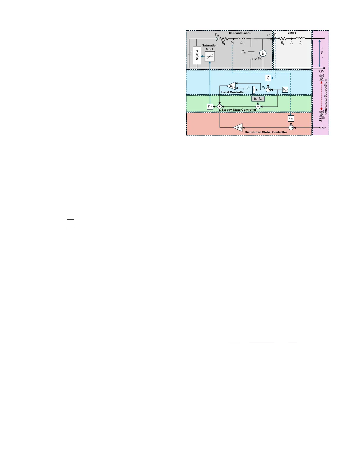
Dissipativity-Based Distrib uted Control and Communication T opology Co-Design for Nonlinear DC Microgrids Mohammad Jav ad Najaﬁrad and Shirantha W elikala Abstract — This paper presents a dissipativity-based dis- tributed droop-fr ee control and communication topology co- design framework for voltage regulation and current sharing in nonlinear DC micr ogrids (MGs), wher e ZIP loads and voltage source con verter (VSC) input saturation constitute the primary nonlinear challenges. ZIP loads introduce a destabilizing nonlinearity through their constant power load (CPL) component, while VSC input saturation imposes hard amplitude constraints on the voltage command signals applied to each distributed generator (DG), collectively making the control design signiﬁcantly more challenging. Achieving simul- taneous voltage regulation and curr ent sharing while jointly co-designing the local controll ers and communication topology under both nonlinearities is the central problem addressed in this work. T o this end, the DC MG is modeled as a networked system of DGs, transmission lines, and ZIP loads coupled through a static interconnection matrix. Each DG is equipped with a local PI-based controller and a distributed consensus- based global contr oller , fr om which a nonlinear network ed error dynamics model is derived. The CPL nonlinearity and the VSC saturation are each characterized via sector-boundedness, where the latter is handled through a dead-zone decompo- sition. Both nonlinearities are simultaneously absorbed into the dissipativity analysis using the S-procedur e and Y oung’s inequality , certifying an IF-OFP property for each DG subsys- tem. Subsequently , controller gains, passivity indices, and the communication topology are co-designed by solving locally and globally formulated Linear Matrix Inequality (LMI) problems. Necessary feasibility conditions are identiﬁed and embedded into the local LMI problems, enabling a one-shot co-design algorithm that avoids iterative procedures. The effectiveness of the proposed framework is validated through simulation of an islanded DC MG under multiple operating scenarios, demonstrating r obust performance superior to con ventional control approaches. Index T erms — Nonlinear DC Microgrid, ZIP Loads, V olt- age Regulation, Input Saturation, Distributed Control, Dissipativity-Based Control. I . I N T RO D U C T I O N The rapid proliferation of renewable energy resources and DC-native loads has fundamentally reshaped modern power systems, positioning DC microgrids (DC MGs) as a cornerstone technology for next-generation distributed energy infrastructure [1]. Unlike A C systems, DC MGs eliminate unnecessary po wer con version stages and remove the complexity of frequency regulation, which results in superior efﬁciency , reduced hardware cost, and simpliﬁed system architecture [2]. Applications such as data centers, electric vehicle charging stations, LED lighting, and con- sumer electronics have further accelerated the adoption of The authors are with the Department of Electrical and Computer Engi- neering, School of Engineering and Science, Stevens Institute of T echnology , Hoboken, NJ 07030, { mnajafir,swelikal } @stevens.edu . DC MGs as a practical and economically viable solution for modern energy networks. Nevertheless, the fast closed-loop dynamics inherent to DC MGs place signiﬁcant demands on the control system, and the presence of heterogeneous loads and distributed generation units introduces nonlinearities and uncertainties that render classical control techniques insuf- ﬁcient. Consequently , the dev elopment of rob ust, scalable, and theoretically rigorous control frameworks for DC MGs has become a subject of considerable research interest in the power systems and control communities [3], [4]. The two primary control objecti ves in DC MGs are v oltage regulation and current sharing. Centralized control strategies, while effecti ve in achieving these objectives, suffer from a single point of failure and lack scalability [3]. Decentralized approaches eliminate the need for inter-DG communica- tion, yet the absence of coordination fundamentally com- promises current sharing accuracy [4]. Distributed control, by contrast, allows each DG to exchange state information with its neighbors over a communication network, and has demonstrated a superior ability to achie ve both objectiv es simultaneously [5]. W ithin distributed control, droop-based methods remain the most widely adopted solution in the literature. Ho wev er , droop control introduces an inherent trade-off between voltage regulation and current sharing, and its performance is sensiti ve to line impedance mismatch and droop coef ﬁcient selection [6]. These fundamental limitations hav e motiv ated a shift toward droop-free distributed control strategies, which rely entirely on inter -DG communication to coordinate voltage and current objectives without the structural compromises of droop mechanisms [7], [8]. A fundamental challenge in the control of DC MGs is the presence of generic ZIP (constant impedance (Z), constant current (I), and constant power (P)) loads. Among the three load components, the constant po wer load (CPL) is of particular concern due to its negati ve incremental impedance characteristic, which introduces a destabilizing nonlinearity into the closed-loop system dynamics [9]. Unlike resistive or constant current loads, a CPL demands a ﬁxed power lev el regardless of the terminal voltage, effecti v ely creating a positiv e feedback mechanism that counteracts the damping of the system and can drive it tow ard instability under certain operating conditions [10]. This destabilizing effect becomes more pronounced as the CPL power lev el increases relative to the total system capacity , making its treatment a critical aspect of any robust control design for DC MGs [11]. The nonlinear nature of CPLs poses signiﬁcant challenges to both stability analysis and controller synthesis, and has motiv ated a substantial body of research focused on developing ad- vanced nonlinear control techniques to ensure reliable DC MG operation in the presence of such loads [12]. Beyond CPLs, the VSCs that interface each DG with the DC bus introduce an additional and practically signiﬁcant nonlinearity in the form of input saturation. In practice, ev ery VSC operates within a ﬁnite voltage command range imposed by its physical design and safety constraints, and the voltage command signal applied to each DG is therefore subject to hard amplitude limits [13]. When these limits are activ e, the actual control input deviates from its intended value, and a controller that does not explicitly account for this discrepancy can exhibit signiﬁcant performance degradation or ev en closed-loop instability [14]. The treatment of input saturation as a sector-bounded nonlinearity via a dead-zone decomposition has been established as a systematic and LMI-compatible approach in the broader nonlinear control literature [15], yet its integration into a dissipativity-based co-design framework for networked DC MGs remains an open problem that this paper addresses. A further and equally important challenge in the design of distributed controllers for DC MGs is the joint optimization of the controller parameters and the communication topol- ogy . In conv entional design approaches, the communication network structure is treated as a ﬁxed and predeﬁned entity , determined independently of the control objectives [3]. This sequential design philosophy , ho wev er , fails to exploit the inherent coupling between network connectivity and closed- loop performance, and can result in either over -provisioned communication infrastructure or degraded control perfor- mance [16]. Recent advances in reconﬁgurable communica- tion technologies have eliminated the necessity for ﬁxed net- work structures, creating new opportunities to co-design the controller and topology in a uniﬁed optimization frame work [17]. Sev eral approaches to this co-design problem hav e been proposed in the literature, including graph-theoretic meth- ods and con ve x optimization-based formulations [18], [19]. Nev ertheless, these approaches typically rely on sequential or iterativ e procedures that treat control and communication objectiv es separately , and do not provide a uniﬁed one- shot co-design strategy that simultaneously and rigorously accounts for the nonlinear dynamics introduced by CPLs and VSC input saturation. This gap motiv ates the uniﬁed dissipativity-based co-design framew ork dev eloped in this paper . T o address the aforementioned challenges in a uniﬁed and rigorous manner, this paper adopts dissipativity theory as the central analytical framew ork. Dissipativity theory offers a powerful and ﬂexible foundation for the analysis and synthesis of robust control systems for large-scale networked systems, as it characterizes the input-output energy behavior of each subsystem without requiring explicit knowledge of the global system dynamics [20]. By focusing on the fun- damental energy exchanges between interconnected subsys- tems, dissipativity-based approaches can certify stability and robustness of the overall networked system ev en when indi- vidual subsystems exhibit complex nonlinear behaviors [21]. Crucially , the dissipativity framework is compatible with LMI-based synthesis tools, which enables the formulation of computationally tractable con ve x optimization problems for controller design. The sector-bounded characterizations of both the CPL nonlinearity and the VSC input saturation are naturally accommodated within this framew ork through the S-procedure and Y oung’ s inequality , allowing both non- linearities to be handled simultaneously without sacriﬁcing the conv exity of the resulting synthesis conditions. This combination of theoretical rigor , computational tractability , and ability to handle multiple nonlinearities makes dissipa- tivity theory a particularly well-suited tool for the co-design problem considered in this paper . In this paper , a dissipati vity-based hierarchical distributed control framework is proposed to simultaneously achiev e voltage regulation and current sharing in DC MGs subject to ZIP loads and VSC input saturation. The DC MG is modeled as a networked system of DGs, transmission lines, and ZIP loads, interconnected through a static matrix that captures the physical coupling structure of the system. A hierarchi- cal controller comprising steady-state, local, and distributed global components is developed for each DG, and a thorough equilibrium analysis is conducted to identify the operating point and establish the feasibility conditions on the saturation constraints. The closed-loop error dynamics of the DC MG are then deri ved as a nonlinear networked error system, incorporating both disturbance inputs and regulated perfor- mance outputs to ensure robust achievement of the desired control objecti ves. The CPL nonlinearity and the VSC input saturation are each characterized via sector -boundedness, and both are simultaneously incorporated into the dissipati vity analysis through the S-procedure and Y oung’ s inequality , certifying an input feedforward output feedback passi vity (IF-OFP) property for each DG subsystem. Building on this, the controller gains, passi vity indices, and communication topology are co-designed by solving a set of locally and globally formulated LMI problems. T o support the feasi- bility of the global LMI problem, necessary conditions are systematically identiﬁed and embedded into the local LMI problems, yielding a tractable one-shot co-design procedure that avoids iterativ e schemes [22]. The main contributions of this paper can be summarized as follows: 1) W e formulate the DC MG control problem as a net- worked system control problem and propose a no vel hi- erarchical droop-free control frame work that combines local steady-state and voltage regulation controllers with distrib uted global consensus-based current sharing controllers. 2) W e incorporate a generic ZIP load model and dev elop a systematic technique to handle the destabilizing CPL nonlinearity via sector-boundedness and the S- procedure, without sacriﬁcing the LMI con ve xity of the overall design framework. 3) W e explicitly model VSC input saturation via a dead- zone decomposition, establish its sector-bounded char- acterization, and incorporate it into the dissipativity analysis through Y oung’ s inequality , handling both nonlinearities simultaneously within a uniﬁed frame- work. 4) W e formulate the ov erall control and topology co- design problem as a set of local and global LMI problems to be executed in one shot, with necessary conditions embedded into the local problems to support global feasibility and avoid iterativ e procedures. The remainder of this paper is structured as follo ws. The essential concepts of dissipativity theory and networked systems are presented in Sec. II to establish the theoreti- cal foundation. The DC MG model with detailed physical topology and component dynamics is introduced in Sec. III. A novel hierarchical control architecture that eliminates traditional droop mechanisms is dev eloped in Sec. IV, where the equilibrium analysis and VSC saturation feasibility con- ditions are also established. The nonlinear networked error dynamics, incorporating both CPL and VSC input saturation nonlinearities, are derived in Sec. V. The dissipativity-based methodology for controller and communication topology co-design, including the extended LMI formulations that account for both nonlinearities, is presented in Sec. VI. Numerical simulations demonstrating the effecti veness of the proposed framework under multiple operating scenarios, in- cluding saturation-acti ve conditions, are provided in Sec. VII. Finally , Sec. VIII offers concluding remarks and directions for future research. I I . P R E L I M I NA R I E S A. Notations The notation R and N signify the sets of real and natural numbers, respectiv ely . For any N ∈ N , we deﬁne N N ≜ { 1 , 2 , .., N } . An n × m block matrix A is denoted as A = [ A ij ] i ∈ N n ,j ∈ N m . Either subscripts or superscripts are used for indexing purposes, e.g., A ij ≡ A ij . [ A ij ] j ∈ N m and diag ([ A ii ] i ∈ N n ) represent a block row matrix and a block diagonal matrix, respectively . 0 and I , respectiv ely , are the zero and identity matrices (dimensions will be clear from the context). A symmetric positi v e deﬁnite (semi-deﬁnite) matrix A ∈ R n × n is denoted by A > 0 ( A ≥ 0) . The symbol ⋆ represents conjugate blocks inside block symmetric matrices. H ( A ) ≜ A + A ⊤ , 1 {·} is the indicator function and 1 N is a vector in R N containing only ones. B. Dissipativity Consider a nonlinear dynamic system: ˙ x ( t ) = f ( x ( t ) , u ( t )) , y ( t ) = h ( x ( t ) , u ( t )) , (1) where x ( t ) ∈ R n , u ( t ) ∈ R q , y ( t ) ∈ R m , and f : R n × R q → R n and h : R n × R q → R m are continuously differentiable and f ( 0 , 0 ) = 0 and h ( 0 , 0 ) = 0 . Deﬁnition 1: [20] The system (1) is dissipati ve under supply rate s : R q × R m → R if there exists a con- tinuously differentiable storage function V : R n → R such that V ( x ) > 0 , ∀ x  = 0 , V ( 0 ) = 0 , and ˙ V ( x ) = ∇ x V ( x ) f ( x, u ) ≤ s ( u, y ) , for all ( x, u ) ∈ R n × R q . 𝑤 𝑧 Σ 𝑖 𝑖 ∈ ℕ 𝑁 𝑀 𝑦 𝑢 ത Σ 𝑖 𝑖 ∈ ℕ ഥ 𝑁 ത 𝑦 ത 𝑢 Fig. 1. A generic networked system Σ . Deﬁnition 2: The system (1) is X -dissipative if it is dissipativ e under the quadratic supply rate: s ( u, y ) ≜  u y  ⊤  X 11 X 12 X 21 X 22   u y  . Remark 1: The system (1) is X -dissipati v e with speciﬁc properties depending on the structure of X [23]: 1) passive, if X =  0 1 2 I 1 2 I 0  ; 2) IF-OFP( ν , ρ ), if X =  − ν I 1 2 I 1 2 I − ρ I  , where ν and ρ are the input and output passivity indices, respectiv ely; 3) L 2 G ( γ ) , if X =  γ 2 I 0 0 − I  , where γ is the L 2 -gain. If the system (1) is linear time-in v ariant (L TI), a necessary and sufﬁcient condition for X -dissipative is provided in the following proposition as a linear matrix inequality (LMI) problem. Proposition 1: [24] The L TI system ˙ x ( t ) = Ax ( t ) + B u ( t ) , y ( t ) = C x ( t ) + D u ( t ) , is X -dissipative if and only if there exists P > 0 such that h −H ( P A ) + C ⊤ X 22 C − P B + C ⊤ X 21 + C ⊤ X 22 D ⋆ X 11 + H ( X 12 D ) + D ⊤ X 22 D i ≥ 0 . C. Networked Systems Consider the networked system Σ in Fig. 1, consisting of dynamic subsystems Σ i , i ∈ N N , ¯ Σ i , i ∈ N ¯ N and a static interconnection matrix M that characterizes interconnections among subsystems, exogenous inputs w ( t ) ∈ R r (e.g. distur- bances) and interested outputs z ( t ) ∈ R l (e.g. performance). The dynamics of each subsystem Σ i , i ∈ N N are giv en by ˙ x i ( t ) = f i ( x i ( t ) , u i ( t )) , y i ( t ) = h i ( x i ( t ) , u i ( t )) , (2) where x i ( t ) ∈ R n i , u i ( t ) ∈ R q i , y i ( t ) ∈ R m i and f i ( 0 , 0 ) = 0 and h i ( 0 , 0 ) = 0 . In addition, each subsystem Σ i is assumed to be X i -dissipativ e , where X i ≜ [ X kl i ] k,l ∈ N 2 . Regarding each subsystem ¯ Σ i , i ∈ N ¯ N , we use similar assumptions and notations, but include a bar symbol to distinguish between the two types of subsystems, e.g., ¯ Σ i is assumed to be ¯ X i -dissipativ e where ¯ X i ≜ [ ¯ X kl i ] k,l ∈ N 2 . Deﬁning u ≜ [ u ⊤ i ] ⊤ i ∈ N N , y ≜ [ y ⊤ i ] ⊤ i ∈ N N , ¯ u ≜ [ ¯ u ⊤ i ] ⊤ i ∈ N ¯ N and ¯ y ≜ [ y ⊤ i ] ⊤ i ∈ N ¯ N , the interconnection matrix M and the corresponding interconnection relationship are given by  u ¯ u z  = M  y ¯ y w  ≡  M uy M u ¯ y M uw M ¯ uy M ¯ u ¯ y M ¯ uw M zy M z ¯ y M zw   y ¯ y w  . (3) The following proposition exploits the X i -dissipativ e and ¯ X i -dissipativ e properties of the subsystems Σ i , i ∈ N N and ¯ Σ i , i ∈ N ¯ N to formulate an LMI problem for synthesizing the interconnection matrix M (3), ensuring the networked system Σ is Y -dissipative for a prespeciﬁed Y under two mild assumptions [25]. Assumption 1: For the networked system Σ , the provided Y -dissipativ e speciﬁcation is such that Y 22 < 0 . Remark 2: Based on Rm. 1, As. 1 holds if the networked system Σ must be either: (i) L2G( γ ) or (ii) IF-OFP( ν , ρ ) with some ρ > 0 , i.e., L 2 -stable or passi ve, respectively . Therefore, As. 1 is mild since it is usually preferable to make the networked system Σ either L 2 -stable or passive. Assumption 2: In the network ed system Σ , each subsys- tem Σ i is X i -dissipativ e with X 11 i > 0 , ∀ i ∈ N N , and similarly , each subsystem ¯ Σ i is ¯ X i -dissipativ e with ¯ X 11 i > 0 , ∀ i ∈ N ¯ N . Remark 3: According to Rm. 1, As. 2 holds if a subsys- tem Σ i , i ∈ N N is either: (i) L2G( γ i ) or (ii) IF-OFP( ν i , ρ i ) with ν i < 0 (i.e., L 2 -stable or non-passiv e). Since in passivity-based control, often the in volved subsystems are non-passiv e (or can be treated as such), As. 2 is also mild. Proposition 2: [25] Under As. 1-2, the network system Σ can be made Y -dissipativ e (from w ( t ) to z ( t ) ) by synthe- sizing the interconnection matrix M (3) via solving the LMI problem: Find: L uy , L u ¯ y , L uw , L ¯ uy , L ¯ u ¯ y , L ¯ uw , M z y , M z ¯ y , M z w , Sub . to: p i ≥ 0 , ∀ i ∈ N N , ¯ p l ≥ 0 , ∀ l ∈ N ¯ N , and (5) , (4) with  M uy M u ¯ y M uw M ¯ uy M ¯ u ¯ y M ¯ uw  = " X 11 p 0 0 ¯ X 11 ¯ p # − 1  L uy L u ¯ y L uw L ¯ uy L ¯ u ¯ y L ¯ uw  . where X kl p ≜ diag ( { p i X kl i : i ∈ N N } ) , ∀ k , l ∈ N 2 , X 12 ≜ diag (( X 11 i ) − 1 X 12 i : i ∈ N N ) , and X 21 ≜ ( X 12 ) ⊤ (terms ¯ X kl ¯ p , ¯ X 12 and ¯ X 21 hav e analogous deﬁnitions). Before concluding this section, we recall three linear algebraic results that will be useful in the sequel. Lemma 1: (Schur Complement) For matrices P > 0 , Q and R , the following statements are equiv alent: 1)  P Q Q ⊤ R  ≥ 0 , (6a) 2) P ≥ 0 , R − Q ⊤ P − 1 Q ≥ 0 , (6b) 3) R ≥ 0 , P − QR − 1 Q ⊤ ≥ 0 . (6c) Pr oof: W e ﬁrst establish the equi valence of (6a) and (6b). Let z =  z 1 z 2  ⊤ be any non-zero vector . Then: z ⊤  P Q Q ⊤ R  z = z ⊤ 1 P z 1 + z ⊤ 1 Qz 2 + z ⊤ 2 Q ⊤ z 1 + z ⊤ 2 Rz 2 (7) Let y = z 2 + P − 1 Qz 1 . Then (7) can be rewritten as: z ⊤ 1 P z 1 − z ⊤ 1 QP − 1 Qz 1 + y ⊤ ( R − Q ⊤ P − 1 Q ) y (8) For the ﬁrst part z ⊤ 1 P z 1 − z ⊤ 1 QP − 1 Qz 1 , we can observe that when P > 0 : z ⊤ 1 P z 1 − z ⊤ 1 QP − 1 Qz 1 = z ⊤ 1 ( P − QP − 1 Q ) z 1 = z ⊤ 1 P 1 / 2 ( I − P − 1 / 2 QP − 1 Q ⊤ P − 1 / 2 ) P 1 / 2 z 1 . (9) Since P − 1 / 2 QP − 1 Q ⊤ P − 1 / 2 is positive semideﬁnite, its eigen v alues are non-negati v e. Therefore, ( I − P − 1 / 2 QP − 1 Q ⊤ P − 1 / 2 ) has eigenv alues less than or equal to 1, making this term positiv e semideﬁnite. Consequently , z ⊤ 1 P z 1 − z ⊤ 1 QP − 1 Qz 1 ≥ 0 . Thus, the entire expression (9) is non-negati v e if and only if R − Q T P − 1 Q ≥ 0 . This establishes the equiv alence of (6a) and (6b). The equi valence of (6a) and (6c) can be established by following similar steps. Lemma 2: For any P > 0 and a square matrix Q : Q ⊤ P − 1 Q ≥ Q ⊤ + Q − P. Pr oof: For any arbitrary matrix S , since P > 0 : we hav e ( S − I ) ⊤ P ( S − I ) ≥ 0 , which simpliﬁes to S ⊤ P S − P S − S ⊤ P + P ≥ 0 . The required result follows by applying the change of vari- ables S = P − 1 Q and rearranging the terms, with equality holding if and only if Q = P . Lemma 3: For an inv ertible R ∈ R n × n and ρ ∈ R > 0 : ( R + ρ I ) − 1 = R − 1 − ρR − 1  I + ρR − 1  − 1 R − 1 . Pr oof: The result follo ws directly from applying the well-known W oodbury Matrix Identity: ( R + U V T ) − 1 = R − 1 − R − 1 U  I + V T R − 1 U  − 1 V T R − 1 with the choices U = √ ρ I and V = √ ρ I . Lemma 4: ( Matrix S-Lemma , [21]) Let Π and Γ be symmetric matrices. If there exists ζ such that ζ ⊤ Γ ζ > 0 , then: ζ ⊤ Γ ζ ≥ 0 = ⇒ ζ ⊤ Π ζ ≥ 0 , ∀ ζ , (10) if and only if there exists λ ≥ 0 such that: Π − λ Γ ≥ 0 . (11) I I I . P RO B L E M F O R M U L A T I O N This section presents the dynamic modeling of the DC MG, which consists of multiple DGs, loads, and transmission lines. Speciﬁcally , our modeling approach is motiv ated by [26], which highlights the role and impact of communication and physical topologies in DC MGs. A. DC MG Physical Inter connection T opology The physical interconnection topology of a DC MG is modeled as a directed connected graph G p = ( V , E ) where V ≜ D ∪ L is bipartite: D ≜ { Σ DG i , i ∈ N N } (DGs) and L ≜ { Σ line l , l ∈ N L } (lines). The DGs are interconnected with each other through transmission lines. The interface between each DG and the DC MG is through a point of common coupling (PCC). For simplicity , the loads are assumed to be      X 11 p 0 0 L uy L u ¯ y L uw 0 ¯ X 11 ¯ p 0 L ¯ uy L ¯ u ¯ y L ¯ uw 0 0 − Y 22 − Y 22 M zy − Y 22 M z ¯ y Y 22 M zw L ⊤ uy L ⊤ ¯ uy − M ⊤ zy Y 22 − L ⊤ uy X 12 − X 21 L uy − X 22 p − X 21 L u ¯ y − L ⊤ ¯ uy ¯ X 12 − X 21 L uw + M ⊤ zy Y 21 L ⊤ u ¯ y L ⊤ ¯ u ¯ y − M ⊤ z ¯ y Y 22 − L ⊤ u ¯ y X 12 − ¯ X 21 L ¯ uy − ( L ⊤ ¯ u ¯ y ¯ X 12 + ¯ X 21 L ¯ u ¯ y + ¯ X 22 ¯ p ) − ¯ X 21 L ¯ uw + M ⊤ z ¯ y Y 21 L ⊤ uw L ⊤ ¯ uw − M ⊤ zw Y 22 − L ⊤ uw X 12 + Y 12 M zy − L ⊤ ¯ uw ¯ X 12 + Y 12 M z ¯ y M ⊤ zw Y 21 + Y 12 M zw + Y 11      > 0 (5) connected to the DG terminals at the respective PCCs [27]. Indeed loads can be mov ed to PCCs using Kron reduction ev en if they are located elsewhere [27]. T o represent the DC MG’ s physical topology , we use its bi-adjacency matrix A ≜ h 0 B B ⊤ 0 i , where B ∈ R N × L is the incident matrix of the DG network (where nodes are just the DGs and edges are just the transmission lines). Note that B is also known as the “bi-adjacency” matrix of G p that describes the connectivity between its tw o types of nodes. In particular , B ≜ [ B il ] i ∈ N N ,l ∈ N L with B il ≜ 1 { l ∈E + i } − 1 { l ∈E − i } , where E + i and E − i represent the out- and in-neighbors of Σ DG i , respectiv ely . B. Dynamic Model of a Distributed Generator (DG) Each DG consists of a DC voltage source, a voltage source conv erter (VSC), and some RLC components. Each DG Σ DG i , i ∈ N N supplies power to a speciﬁc ZIP load at its PCC (denoted PCC i ). Additionally , it interconnects with other DG units via transmission lines { Σ line l : l ∈ E i } . Figure 2 illustrates the schematic diagram of Σ DG i , including the local ZIP load, a connected transmission line, and the steady state, local, and distributed global controllers. By applying Kirchhoff ’ s Current Law (KCL) and Kirch- hoff ’ s V oltage Law (KVL) at PCC i on the DG side, we get the following equations for Σ DG i , i ∈ N N : Σ DG i : ( C ti dV i dt = I ti − I Li ( V i ) − I i + w v i , L ti dI ti dt = − V i − R ti I ti + sat ( V ti ) + w ci , (12) where the parameters R ti , L ti , and C ti represent the inter- nal resistance, internal inductance, and ﬁlter capacitance of Σ DG i , respectiv ely . The state variables are selected as V i and I ti , where V i is the PCC i voltage and I ti is the internal current. Moreover , sat ( V ti ) is deﬁned as: sat ( V ti ) ≜      V max ti if V ti > V max ti , V ti if V min ti ≤ V ti ≤ V max ti , V min ti if V ti < V min ti , with V min ti and V min ti denoting the lower and upper saturation limits of the VSC of Σ DG i , i ∈ N N , respectiv ely , and V ti is the input command signal applied to the VSC. I Li ( V i ) is the total current drawn by the ZIP load, and I i is the total current injected to the DC MG by Σ DG i . W e ha ve also included w v i and w ci terms in (12) to represent unknown disturbances (assumed bounded and zero mean) resulting from external effects or modeling imperfections. Note that V ti , I Li ( V i ) , and I i terms in (12) are respecti vely determined by the controllers, ZIP loads, and transmission lines at Σ DG i . Their details will be provided in the sequel. Let us begin with the total line current I i , which is given by I i = X l ∈E i B il I l , (13) where I l , l ∈ E i are line currents. C. Dynamic Model of a T ransmission Line As shown in Fig. 2, the po wer line Σ line l can be repre- sented as an RL circuit with resistance R l and inductance + -  VSC - i                             + -         - + Neig h bor in g In for m a t ion     󰇛   󰇜 DG - i a n d L oa d - i Dist r ibu t e d Globa l Con t r oll e r L oca l Con t r oll e r L in e - l + -   +     + St e a dy - St a t e Con t r oll e r S a t u r a t ion B loc k With Sa t ur a t ion       Fig. 2. The electrical schematic of DG- i , load- i , i ∈ N N , local controller, distributed global controller, and line- l , l ∈ N L . L l . By applying KVL to Σ line l , we obtain: Σ line l : n L l dI l dt = − R l I l + ¯ u l + ¯ w l , (14) where I l is the line current (i.e., the state), ¯ u l = V i − V j = P i ∈E l B il V i is the voltage dif ferential (i.e., the line input), and ¯ w l ( t ) represents the unknown disturbance (assumed bounded and zero mean) that affects the line dynamics. D. Dynamic Model of a ZIP Load Recall that I Li ( V i ) in (12) (see also Fig. 2) is the total current drawn by the load at Σ DG i , i ∈ N N . As the load is assumed to be a generic “ZIP” load, I Li ( V i ) takes the form: I Li ( V i ) = I Z Li ( V i ) + I I Li ( V i ) + I P Li ( V i ) . (15) Here, the ZIP load’ s components are: (i) a constant impedance load: I Z Li ( V i ) = Y Li V i , where Y Li = 1 /R Li is the conductance of this load component; (ii) a constant current load: I I Li ( V i ) = ¯ I Li , where ¯ I Li is the current demand of this load component; and (iii) a constant power load (CPL): I P Li ( V i ) = V − 1 i P Li , where P Li represents the power demand of this load component. As opposed to I Z Li ( V i ) and I I Li ( V i ) (that take an af ﬁne linear form in the chosen state variables), the CPL I P Li ( V i ) introduces signiﬁcant stability challenges due to its inherent negati v e impedance characteristic. This can be observed by examining the small-signal impedance of the CPL: Z C P L = ∂ V i ∂ I P Li = ∂ V i ∂ ( P Li /V i ) = − V 2 i P Li < 0 . (16) This negati ve impedance characteristic creates a destabi- lizing effect in the DC MG, as it tends to amplify voltage perturbations rather than dampen them [28]. When a small voltage drop occurs, the CPL draws more current to maintain constant po wer , further reducing the voltage and potentially leading to voltage collapse if not properly controlled. The nonlinear nature of CPLs also introduces complexities for the control design. In particular , the nonlinear term I P Li ( V i ) = V − 1 i P Li appears in the voltage dynamics (not in current dynamics) channel in (12), and hence cannot be di- rectly canceled using state feedback linearization techniques. Consequently , this nonlinearity must be carefully accounted for to ensure system stability and robustness, as often CPLs constitute a signiﬁcant portion of the total ZIP load. As we will see in the subsequent sections, the proposed control framework exploits a ke y structural property of this nonlinearity , namely , its sector boundedness, to address these stability and robustness concerns posed by CPLs. I V . P RO P O S E D H I E R A R C H I C A L C O N T RO L A R C H I T E C T U R E The primary control objectiv e of the DC MG is to ensure that the PCC i voltage V i at each Σ DG i , i ∈ N N closely follows a speciﬁed reference voltage V ri while maintaining a proportional current sharing among DGs (with respect to their power ratings). In the proposed control architecture, these control objectives are achie ved through the comple- mentary action of local and distributed controllers. The local controller at each Σ DG i is a PI controller responsible for the voltage regulation task. On the other hand, the distrib uted global controller at each Σ DG i is a consensus-based controller responsible for ensuring proper current sharing among DGs. A. Local V oltage Re gulating Contr oller At each Σ DG i , i ∈ N N , for its PCC i voltage V i ( t ) to effec- tiv ely track the assigned reference voltage V ri ( t ) , it is imper- ativ e to ensure that the tracking error e i ( t ) ≜ V i ( t ) − V ri ( t ) con ver ges to zero, i.e. lim t →∞ ( V i ( t ) − V ri ) = 0 . T o this end, motiv ated by [29], we ﬁrst include each Σ DG i , i ∈ N N with an integrator state v i deﬁned as v i ( t ) ≜ R t 0 ( V i ( τ ) − V ri ) dτ ) (see also Fig. 2) that follows the dynamics dv i ( t ) dt = e i ( t ) = V i ( t ) − V ri − K aw,i ϕ i ( u i ) , (17) where K aw,i > 0 is the anti-windup gain, with ϕ i ( u i ) being the dead-zone nonlinearity deﬁned as ϕ i ( u i ) ≜      V max ti − u i if u i > V max ti , 0 if V min ti ≤ u i ≤ V max ti , V min ti − u i if u i < V min ti , (18) when saturation is inactive, ϕ i ( u i ) = 0 and (18) reduces to the standard integrator; otherwise, − K aw,i ϕ i ( u i ) prev ents unbounded accumulation of v i . Then, Σ DG i is equipped with a local state feedback con- troller u iL ( t ) ≜ k P i 0 ( V i − V ri ) + k I i 0 v i ( t ) = K i 0 x i ( t ) − k P i 0 V ri , (19) where x i ≜  V i I ti v i  ⊤ , (20) denotes the augmented state (henceforth referred to as the state) of Σ DG i and K i 0 ≜  k P i 0 0 k I i 0  ∈ R 1 × 3 where K i 0 is the local controller gain. B. Distributed Global Contr oller W e implement distributed global controllers at each DG, and task them with maintaining a proportional current shar- ing among the DGs. In particular, their objecti ve is to ensure: I ti ( t ) P ni = I tj ( t ) P nj = I s , ∀ i, j ∈ N N , (21) where P ni and P nj represent the power ratings of DGs Σ DG i and Σ DG j respectiv ely , and I s represents the common current sharing ratio that emerges from balancing the total load demand among DGs according to their power ratings. T o address the current sharing, as sho wn in Fig. 2, we employ a consensus-based distributed controller u iG ( t ) ≜ X j ∈ ¯ F − i k I ij  I ti ( t ) P ni − I tj ( t ) P nj  , (22) where each k I ij ∈ R is a consensus controller gain. Note that we denote the communication topology as a directed graph G c = ( D , F ) where D ≜ { Σ DG i , i ∈ N N } and F represents the set of communication links among DGs. The notations F + i and F − i (see (22)) are deﬁned as the communication-wise out- and in-neighbors, respecti vely . Finally , the overall control input u i ( t ) applied to the VSC of Σ DG i (i.e., as V ti ( t ) in (12)) can be expressed as u i ( t ) ≜ V ti ( t ) = u iS + u iL ( t ) + u iG ( t ) , (23) where u iL is giv en by (19), u iG is giv en by (22) and u iS represents the steady-state control input. As we will see in the sequel, steady-state control input u iS in (23) also plays a crucial role in achieving the desired equi- librium point of the DC MG. In particular , this steady-state component ensures that the system maintains its operating point that satisﬁes both voltage re gulation and current sharing objectiv es. The speciﬁc structure and properties of u iS will be characterized through our stability analysis presented in Sec. V -A. C. Closed-Loop Dynamics of the DC MG By combining (12) and (17), the ov erall dynamics of Σ DG i , i ∈ N N can be written as dV i dt = 1 C ti  I ti − I Li ( V i ) − I i + w v i ( t )  , (24a) dI ti dt = 1 L ti  − V i − R ti I ti + u i + ϕ i ( u i ) + w ci ( t )  , (24b) dv i dt = V i − V ri − K aw,i ϕ i ( u i ) , (24c) where the terms I i , I Li ( V i ) , and u i can be substituted from (13), (15), and (23), respectively . W e can restate (24) as ˙ x i ( t ) = A i x i ( t ) + B i u i ( t ) + B aw i ϕ i ( u i ( t )) + E i d i ( t ) + ξ i ( t ) + g i ( x i ( t )) , (25) where x i ( t ) is the DG state as deﬁned in (20), ϕ i ( u i ( t )) is the dead-zone nonlinearity deﬁned in (18) applied to the VSC input V ti = u i ( t ) , d i ( t ) is the exogenous input (disturbance) deﬁned as: d i ( t ) ≜ ¯ w i + w i ( t ) , (26) with ¯ w i ≜  − ¯ I Li 0 − V ri  ⊤ representing the ﬁxed (mean) known disturbance and w i ( t ) ≜  w v i ( t ) w ci ( t ) 0  ⊤ representing the zero-mean unkno wn disturbance, E i ≜ diag (  C − 1 ti L − 1 ti 1  ) is the disturbance input matrix, ξ i ( t ) is the transmission line coupling input deﬁned as ξ i ( t ) ≜  − C − 1 ti P l ∈E i B il I l ( t ) 0 0  ⊤ , g i ( x i ( t )) represents the                                                                            + +         Fig. 3. DC MG dynamics as a networked system conﬁguration. nonlinear vector ﬁeld due to the CPL deﬁned as g i ( x i ( t )) ≜ C − 1 ti h − P Li V i 0 0 i ⊤ , and A i and B i are system matrices respectively deﬁned as A i ≜   − Y Li C ti 1 C ti 0 − 1 L ti − R ti L ti 0 1 0 0   , B i ≜   0 1 L ti 0   , B aw i ≜   0 1 L ti − K aw,i   . (27) Similarly , using (14), the state space representation of the transmission line Σ Line l can be written in a compact form: ˙ ¯ x l ( t ) = ¯ A l ¯ x l ( t ) + ¯ B l ¯ u l ( t ) + ¯ E l ¯ w l ( t ) , (28) where ¯ x l ≜ I l is the transmission line state, ¯ E l ≜  1 L l  is the disturbance matrix, and ¯ A l and ¯ B l are the system matrices respectiv ely deﬁned as ¯ A l ≜ h − R l L l i and ¯ B l ≜  1 L l  . (29) D. Networked System Model Let us deﬁne u ≜ [ u i ] ⊤ i ∈ N N and ¯ u ≜ [ ¯ u l ] ⊤ l ∈ N L respectiv ely as vectorized control inputs of DGs and lines, x ≜ [ x ⊤ i ] ⊤ i ∈ N N and ¯ x ≜ [ ¯ x l ] ⊤ l ∈ N L respectiv ely as the full states of DGs and lines, w ≜ [ w ⊤ i ] ⊤ i ∈ N N and ¯ w ≜ [ ¯ w l ] ⊤ l ∈ N L respectiv ely as disturbance inputs of DGs and lines. Using these notations, we can now represent the closed- loop DC MG as two sets of subsystems (i.e., DGs and lines) interconnected with disturbance inputs through a static inter- connection matrix M as shown in Fig. 3. From comparing Fig. 3 with Fig. 1, it is clear that the DC MG takes a similar form to a standard networked system discussed in Sec. II-C. T o identify the speciﬁc structure of the interconnection matrix M in Fig. 3 (i.e., for DC MG), we need to closely observe how the dynamics of DGs and lines are intercon- nected and how they are coupled with disturbance inputs. T o this end, we ﬁrst use (25) and (23) to state the closed- loop dynamics of Σ DG i as: ˙ x i ( t ) = ( A i + B i K i 0 ) x i ( t ) + ˜ η i ( t ) , (30) where ˜ η i is deﬁned as ˜ η i ( t ) ≜ E i w i ( t ) + X l ∈E i ¯ C il ¯ x l ( t ) + X j ∈ ¯ F − i K ij x j ( t ) + θ i , (31) with ¯ C il ≜ − C − 1 ti  B il 0 0  ⊤ , θ i ≜ E i ¯ w i + B i u iS − B i k P i 0 V ri , and K ij represents the distributed consensus controller gain matrix (for current sharing objective), that takes the form: K ii ≜ 1 L ti     0 0 0 0 P j ∈F − i k I ij P ni 0 0 0 0     , K ij ≜ 1 L ti    0 0 0 0 − k I ij P nj 0 0 0 0    . (32) From (32), observe that only the (2,2)-th element in each block K ij is non-zero. Let K I ∈ R N × N denote the matrix that contains only these (2,2) block entries, i.e., K I = [ K 2 , 2 ij ] i,j ∈ N N . The controller gain matrix satisﬁes the weighted Laplacian property: K I P n 1 N = 0 , (33) where P n = diag (  P ni  i ∈ N N ) and 1 N ∈ R N is the vector of ones. This ensures that the distributed control vanishes when proportional current sharing is achieved among all DGs. By vectorizing (31) ov er all i ∈ N N , we get ˜ η ≜ E w + ¯ C ¯ x + K x + θ, (34) where ˜ η ≜ [ ˜ η ⊤ i ] ⊤ i ∈ N N represents the effecti v e input vector to the DGs (see Fig. 3), E ≜ diag ([ E i ] i ∈ N N ) represents the disturbance matrix of DGs, ¯ C ≜ [ ¯ C il ] i ∈ N N ,l ∈ N L , K ≜ [ K ij ] i,j ∈ N N , and θ ≜ [ θ i ] ⊤ i ∈ N N represents a constant (time- in v ariant) input vector applied to the DGs. Remark 4: The block matrices K and ¯ C in (34) are indicativ e of the communication and physical topologies of the DC MG, respecti v ely . In particular, the ( i, j ) th block in K , i.e., K ij , indicates a communication link from Σ DG j to Σ DG i . Similarly , ( i, l ) th block in ¯ C , i.e., ¯ C i,l indicates a physical link between Σ DG i and Σ Line l . Similarly to DGs, using (28), we state the closed-loop dynamics of Σ Line l as ˙ ¯ x l ( t ) = ¯ A l ¯ x l ( t ) + ˜ ¯ η l ( t ) , (35) where ˜ ¯ η l ( t ) is deﬁned as ˜ ¯ η l ( t ) ≜ X i ∈E l C il x i ( t ) + ¯ E l ¯ w l ( t ) , (36) with C il ≜  B il 0 0  (note also that C il = − C ti ¯ C ⊤ il ). By vectorizing (36) over all l ∈ N L , we get: ˜ ¯ η ≜ C x + ¯ E ¯ w , (37) where ˜ ¯ η ≜ [ ˜ ¯ η l ] ⊤ l ∈ N L represents the effecti v e input vector to the lines, C ≜ [ C il ] l ∈ N L ,i ∈ N N (note also that C = − ¯ C ⊤ C t where C t ≜ diag ([ C ti I 3 ] i ∈ N N ) ), ¯ E ≜ diag ([ ¯ E l ] l ∈ N L ) , and ¯ w ≜ [ ¯ w l ] l ∈ N L . Finally , using (34) and (37), we can identify the intercon- nection relationship:  ˜ η ⊤ ˜ ¯ η ⊤  ⊤ = M  x ⊤ ¯ x ⊤ w ⊤ ¯ w ⊤  ⊤ , where the interconnection matrix M takes the form: M ≜  K ¯ C E 0 C 0 0 ¯ E  . (38) When the physical topology G p is predeﬁned, so are the block matrices ¯ C and C (recall C = − ¯ C ⊤ C t ). This leav es only the block matrix K inside the block matrix M as a tunable quantity to optimize the desired properties of the closed-loop DC MG system. Note that synthesizing K simultaneously determines the distributed global controllers (22) and the communication topology G c . In the follo wing two sections, we formulate this networked system’ s error dynamics (around a desired operating point) and pro vide a systematic dissipativity-based approach to synthesize this block matrix K to enforce dissipativity of the closed-loop error dynamics (from disturbance inputs to a given perfor- mance output). V . N O N L I N E A R N E T W O R K E D E R R O R D Y N A M I C S This section establishes the mathematical foundation for the stability and robustness analysis of the DC MG with ZIP loads. First, a rigorous equilibrium point analysis is conducted to characterize steady-state behavior and deriv e necessary conditions for simultaneous voltage regulation and current sharing. Next, nonlinear error dynamics are dev eloped around the identiﬁed equilibrium point, explicitly accounting for CPL characteristics. These error dynamics are then cast into a standard networked system structure with clearly deﬁned performance outputs and disturbance inputs, providing a complete state-space representation of both DG and transmission line error subsystems. This formulation serves as the foundation for the dissipativity-based control design presented in the next section. A. Equilibrium P oint Analysis of the DC MG In this section, we analyze the equilibrium conditions of the DC MG to establish mathematical relationships between system parameters and steady-state behavior . This analysis is crucial for identifying the necessary conditions for si- multaneously achieving voltage regulation and proportional current sharing. W e pay particular attention to the impact of CPL components, which introduce nonlinear dynamics and potentially lead to instability in the DC MG system. Lemma 5: Assuming all zero mean unkno wn disturbance components to be zero, i.e., w i ( t ) = 0 , ∀ i ∈ N N and ¯ w l ( t ) = 0 , ∀ l ∈ N L , for a giv en reference voltage vector V r , under a ﬁxed control input u ( t ) = u E ≜ [ u iE ] i ∈ N N deﬁned as u E ≜ [ I + R t ( B R − 1 B ⊤ + Y L )] V r + R t ( ¯ I L + diag ( V r ) − 1 P L ) , (39) there exists an equilibrium point for the DC MG character- ized by reference voltage vector V r ≜ [ V ri ] ⊤ i ∈ N N , constant current load vector ¯ I L ≜ [ ¯ I Li ] i ∈ N N , and CPL vector P L ≜ [ P Li ] ⊤ i ∈ N N , given by: V E = V r , I tE = ( B R − 1 B ⊤ + Y L ) V r + ¯ I L + diag ( V r ) − 1 P L , ¯ I E = R − 1 B ⊤ V r , (40) provided that the equilibrium control input u E satisﬁes the VSC saturation constraints: V min ti ≤ u iE ≤ V max ti , ∀ i ∈ N N , where we deﬁne the state equilibrium vectors V E ≜ [ V iE ] i ∈ N N , I tE ≜ [ I tiE ] i ∈ N N , ¯ I E ≜ [ ¯ I lE ] l ∈ N L , and the system parameters Y L ≜ diag ([ Y Li ] i ∈ N N ) , R t ≜ diag ([ R ti ] i ∈ N N ) , and R ≜ diag ([ R l ] l ∈ N L ) . Pr oof: The equilibrium state of the closed-loop dy- namic Σ DG i (25) satisﬁes: A i x iE ( t ) + B i u iE ( t ) + E i d iE ( t ) + ξ iE ( t ) = 0 , (41) where x iE ≜  V iE I tiE v iE  ⊤ represents the equilibrium state components of DG, and w iE ≜ ¯ w i and ξ iE represent the equilibrium values of disturbance and interconnection terms, respectiv ely . Thus, we get   − Y Li C ti − 1 C ti 0 − 1 L ti − R ti L ti 0 1 0 0     V iE I tiE v iE   +   0 1 L ti 0   u iE + E i ¯ w i + ξ iE = 0 . (42) From respective rows of this matrix equation, we get: 1 C ti − Y Li V iE + I tiE − ¯ I Li − P Li V iE − X l ∈E i B il ¯ I lE ! = 0 , (43) 1 L ti ( − V iE − R ti I tiE + u iE ) = 0 , (44) V iE − V ri = 0 . (45) From the last two equations abov e, we can obtain V iE = V ri , (46) u iE = V iE + R ti I tiE . (47) T o simplify the ﬁrst equation further, we require to know an expression for ¯ I lE . Note that the equilibrium state of the Σ Line l (28) satisﬁes: ¯ A l ¯ x lE ( t ) + ¯ B l ¯ u lE + ¯ E l ¯ w lE ( t ) = 0 , (48) where ¯ x lE ≜ ¯ I lE represents the equilibrium state of line. The ¯ u lE ≜ P i ∈E l B il V iE and ¯ w lE ≜ 0 , respecti vely , represent the equilibrium values of control input and disturbance of lines. Therefore, we get: − R l L l ¯ I lE + 1 L l X i ∈E l B il V iE = 0 , (49) leading to ¯ I lE = 1 R l X i ∈E l B il V iE = 1 R l X j ∈E l B j l V j E , (50) which can be applied in (43) (together with (46)) to obtain − Y Li V ri + I tiE − X l ∈E i B il  1 R l X j ∈E l B j l V rj  − ¯ I Li − P Li V ri = 0 . (51) W e next vectorize these equilibrium conditions. Note that, then the control equilibrium equation (47) becomes: u E = V r + R t I tE . (52) V ectorizing the voltage dynamics equation (51), we get: − Y L V r + I tE − B R − 1 B ⊤ V r − ¯ I L − diag ( V r ) − 1 P L = 0 , leading to I tE = ( B R − 1 B ⊤ + Y L ) V r + ¯ I L + diag ( V r ) − 1 P L . Therefore, the vectorized control equilibrium equation can be expressed as: u E = V r + R t I tE = V r + R t (( B R − 1 B ⊤ + Y L ) V r + ¯ I L + diag ( V r ) − 1 P L ) = [ I + R t ( B R − 1 B ⊤ + Y L )] V r + R t ( ¯ I L + diag ( V r ) − 1 P L ) . For the equilibrium line currents, by vectorizing (50), we get ¯ I E = R − 1 B ⊤ V r . This completes the proof, as we hav e deriv ed all the required equilibrium conditions. Remark 5: The uniqueness is mathematically guaranteed because the diagonal matrices R , R t , and Y L hav e strictly positiv e elements, making them positiv e deﬁnite, while the incidence matrix B maintains full rank by virtue of the connected network topology . Consequently , the coefﬁcient matrix ( B R − 1 B ⊤ + Y L ) in (40) is in vertible, which ensures a unique one-to-one mapping from any giv en reference voltage vector V r to all equilibrium variables under speciﬁed loading conditions. Remark 6: At the equilibrium, we require the condition for proportional current sharing among DGs to meet (i.e., (21)), and thus, we require I tiE P ni = I s ⇐ ⇒ I tiE = P ni I s , ∀ i ∈ N N , (53) which can be expressed in v ectorized form as I tE = P n 1 N I s , where P n ≜ diag ([ P ni ] i ∈ N N ) . Using this require- ment in (52), we get u E = V r + R t P n 1 N I s , i.e., u iE = V ri + R ti P ni I s , ∀ i ∈ N N . Therefore, to achiev e this particular control equilibrium (which satisﬁes both voltage regulation and current sharing objectiv es), we need to select our steady-state control input in (23) as: u iS = V ri + R ti P ni I s , ∀ i ∈ N N . (54) This is because at the equilibrium point, local control u iL (19) and distributed global control u iG (22) components are, by deﬁnition, zero for any i ∈ N N . Furthermore, to ensure the equilibrium control input u iE = u iS does not violate the VSC saturation constraint, we require: V min ti ≤ V ri + R ti P ni I s ≤ V max ti , ∀ i ∈ N N . In conclusion, using Lm. 5 and Rm. 6, for the equilibrium of DC MG to satisfy the voltage regulation and current sharing conditions, we require: u E = [ I + R t ( B R − 1 B ⊤ + Y L )] V r + R t ( ¯ I L + diag ( V r ) − 1 P L ) = V r + R t P n 1 N I s = u S V E = V r , I tE = ( B R − 1 B ⊤ + Y L ) V r + ¯ I L + diag ( V r ) − 1 P L = P n 1 N I s , ¯ I E = R − 1 B ⊤ V r . (55) The following theorem formalizes the optimization prob- lem deriv ed from Lm. 5 and Rm. 6, for the selection of V r and I s , that ensures the existence of an equilibrium state that satisﬁes voltage regulation and current sharing conditions while also respecting reference voltage limits V min and V max and the current sharing coefﬁcient I s ∈ [0 , 1] . A formal proof is omitted as the result follows directly from the equilibrium relationships and the remarks above. Theorem 1: T o ensure the existence of an equilibrium point that satisﬁes the voltage regulation and current sharing objectiv es, the reference voltages V r and current sharing co- efﬁcient I s should be a feasible solution in the optimization problem: min V r ,I s α V ∥ V r − ¯ V r ∥ 2 + α I I s Sub . to: V min ≤ V r ≤ V max , 0 ≤ I s ≤ 1 , (56) P n 1 N I s − ( B R − 1 B ⊤ + Y L ) V r = ¯ I L + diag ( V r ) − 1 P L , V min t ≤ V r + R t P n 1 N I s ≤ V max t , where ¯ V r is a desired reference v oltage v alue, V min t ≜ [ V min ti ] i ∈ N N , V max t ≜ [ V max ti ] i ∈ N N , and α V > 0 and α I > 0 are two normalizing cost coefﬁcients. It is worth noting that the above optimization problem becomes an LMI problem (conv ex) when the CPL is omitted (i.e., when P L = 0 ). This formulation ensures proper system operation through multiple aspects. The equality constraint guarantees that the current sharing objectiv e is achieved across all DG units. The reference voltage bounds maintain system operation within safe and ef ﬁcient limits through the inequality constraints on V r . Furthermore, the constraint on I s ensures that the current sharing coefﬁcient remains properly normalized for practical implementations. As stated earlier , the nonlinear term diag ( V r ) − 1 P L introduces addi- tional complexity in determining a feasible set of reference voltages and a current sharing coefﬁcient that simultaneously satisfy voltage regulation and current sharing objectiv es. B. Nonlinear Err or Dynamics with CPL The network system representation described in Sec. IV -D can be simpliﬁed by considering the error dynamics around the identiﬁed equilibrium point in Lm. 5. As we will see in the sequel, the resulting error dynamics can be seen as a networked system (called the networked error system) comprised of DG error subsystems, line error subsystems, external disturbance inputs, and performance outputs. W e ﬁrst deﬁne error variables that capture de viations from the identiﬁed equilibrium: ˜ V i = V i − V iE = V i − V ri , (57a) ˜ I ti = I ti − I tiE = I ti − P ni I s , (57b) ˜ v i = v i − v iE , (57c) ˜ I l = I l − ¯ I lE = I l − 1 R l X i ∈E l B il V ri . (57d) Now , considering the dynamics (24a)-(24c), equilibrium point established in Lm. 5, and the proposed a hierarchical control strategy u i ( t ) (23), the error dynamics can then be deriv ed as follows. The voltage error dynamics can be derived using (24a) and (57a) as: ˙ ˜ V i = − Y Li C ti ( ˜ V i + V ri ) + 1 C ti ( ˜ I ti + P ni I s ) − 1 C ti ¯ I Li − 1 C ti X l ∈E i B il ( ˜ I l + 1 R l X j ∈E l B j l V rj ) − 1 C ti ( ˜ V i + V ri ) − 1 P Li + 1 C ti w v i ≡ 1 C ti  ϕ V + ψ V + g i ( ˜ V i )  + 1 C ti w v i , (58) where ϕ V ≜ − Y Li ˜ V i + ˜ I ti − X l ∈E i B il ˜ I l , (59a) ψ V ≜ − Y Li V ri + P ni I s − ¯ I Li − X l ∈E i B il R l X j ∈E l B j l V rj − V ri P Li , (59b) g i ( ˜ V i ) ≜ V − 1 ri P Li − ( ˜ V i + V ri ) − 1 P Li . (59c) The current error dynamics can be obtained using (24b) and (57b) as: ˙ ˜ I ti = − 1 L ti ( ˜ V i + V ri ) − R ti L ti ( ˜ I ti + P ni I s ) + 1 L ti ( u iS + k P i 0 ˜ V i + k I io ˜ v i + X j ∈ ¯ F − i k ij ( ˜ I ti P ni − ˜ I tj P nj )) + 1 L ti w ci , ≡ 1 L ti  ϕ I + ψ I  + 1 L ti w ci , (60) where ϕ I ≜ − ˜ V i − R ti ˜ I ti + k p io ˜ V i + k I io ˜ v i + X j ∈ ¯ F − i k ij ( ˜ I ti P ni − ˜ I tj P nj )) , (61a) ψ I ≜ − V ri − R ti P ni I s + u iS . (61b) The inte gral error dynamics can be achie v ed by using (24c) and (57c) as: ˙ ˜ v i = ˜ V i − K aw,i ϕ i ( u i ) , (62) where ϕ i ( u i ) denotes the dead-zone of the scalar VSC command u i ∈ R (19). Since the feasibility condition in Th. 1 ensures V min ti ≤ u iE ≤ V max ti , we hav e ϕ i ( u iE ) = 0 and thus ϕ i ( u i ) = ϕ i ( u i − u iE ) at equilibrium. It is worth noting that, as a consequence of the equilibrium analysis and the steady state control input selection (see (53) and (54)), the terms Ψ V (59b) and Ψ I (61b) are canceled. Therefore, for each DG error subsystem ˜ Σ DG i , i ∈ N N , we hav e an error state vector ˜ x i =  ˜ V i , ˜ I ti , ˜ v i  ⊤ with the dynamics: ˙ ˜ x i = ( A i + B i K i 0 ) ˜ x i + g i ( ˜ x i ) + B aw i ϕ i ( u i ) + ˜ u i , (63) where ˜ u i represents the interconnection input deﬁned as ˜ u i = X l ∈E i ¯ C il ˜ ¯ x l + X j ∈ ¯ F − i K ij ˜ x j + E i w i , (64) and g i ( ˜ x i ) is the nonlinear vector due to the CPL, deﬁned as g i ( ˜ x i ) =   1 C ti  V − 1 ri P Li − ( ˜ V i + V ri ) − 1 P Li  0 0   , (65) with A i and B i as deﬁned in (27). Follo wing similar steps, we can obtain the dynamics of the transmission line error subsystem ˜ Σ Line l , l ∈ N L as: ˙ ˜ ¯ x l = ¯ A l ˜ ¯ x l + ˜ ¯ u l , (66) where ˜ ¯ u l represents the line interconnection input inﬂuenced by DG voltages and disturbances: ˜ ¯ u l = ¯ u l + ¯ E l ¯ w l = X i ∈E l B il ˜ V i + ¯ E l ¯ w l . (67) T o ensure robust stability (dissipativity) of this networked error system, we deﬁne local performance outputs as follo ws. For each DG error subsystem ˜ Σ DG i , i ∈ N N , we deﬁne the performance output as: z i ( t ) ≜ H i ˜ x i ( t ) , (68) where H i can be selected as H i ≜ I , ∀ i ∈ N N (not necessar- ily). Similarly , for each line error subsystem ˜ Σ Line l , l ∈ N L , we deﬁne the performance output as: ¯ z l ( t ) ≜ ¯ H l ˜ ¯ x l ( t ) , (69) where ¯ H l can be selected as ¯ H l ≜ I , ∀ l ∈ N L (not necessarily). Upon vectorizing these performance outputs ov er all i ∈ N N and l ∈ N L (respectiv ely), we obtain: z ≜ H ˜ x and ¯ z ≜ ¯ H ˜ ¯ x, (70) where H ≜ diag ([ H i ] i ∈ N N ) and ¯ H ≜ diag ([ ¯ H l ] l ∈ N L ) . This choice of performance output mapping provides a direct correspondence between error subsystem states and the performance outputs. Deﬁning z ≜  z ⊤ i  ⊤ i ∈ N N and ¯ z ≜  ¯ z ⊤ l  ⊤ l ∈ N L , we consoli- date the performance outputs and disturbance inputs as z c ≜  z ⊤ ¯ z ⊤  ⊤ and w c ≜  w ⊤ ¯ w ⊤  ⊤ . (71) The consolidated disturbance vector w c affects the netw orked error dynamics, particularly the DG error subsystems and the line error subsystems, respectiv ely , through the consolidated disturbance matrices E c and ¯ E c , deﬁned as: E c ≜  E 0  and ¯ E c ≜  0 ¯ E  . (72) The zero blocks in the E c and ¯ E c indicate that line disturbances do not directly af fect DG error subsystem inputs and vice versa. Analogously , the dependence of consolidated performance outputs on the networked error system states can be described using consolidated performance matrices H c ≜  H 0  and ¯ H c ≜  0 ¯ H  . (73) W ith these deﬁnitions and the deriv ed error subsystem dynamics (63) and (66), it is easy to see that the closed- loop error dynamics of the DC MG can be modeled as a networked error system as shown in Fig. 4. In there, the interconnection relationship between the error subsystems, disturbance inputs and performance outputs is described by:  ˜ u ˜ ¯ u z c  ⊤ = M  ˜ x ˜ ¯ x w c  ⊤ , (74) where the interconnection matrix M takes the form: M ≜   M ˜ ux M ˜ u ¯ x M ˜ uw c M ˜ ¯ ux M ˜ ¯ u ¯ x M ˜ ¯ uw c M z c x M z c ¯ x M z c w c   ≡   K ¯ C E c C 0 ¯ E c H c ¯ H c 0   . (75) V I . D I S S I P A T I V I T Y - B A S E D C O - D E S I G N F R A M E W O R K F O R C O N T RO L L E R S A N D C O M M U N I C A T I O N T O P O L O G Y In this section, we ﬁrst introduce the global control and topology co-design problem for the DC MG using the deriv ed networked error dynamics representation in the previous section (see Fig. 4). As this co-design problem exploits dissipativity properties of the in v olved subsystem error dynamics, we next identify necessary conditions for                                                                                                      Fig. 4. DC MG error dynamics as a networked system with disturbance inputs and performance outputs. subsystem dissipativity properties. Subsequently , we embed these necessary conditions in the local dissipativ e controller design problems implemented at the subsystems. Finally , the ov erall control design process is summarized. A. Err or Subsystem Dissipativity Properties Consider the DG error subsystem ˜ Σ DG i , i ∈ N N (63) to be X i -dissipativ e with X i =  X 11 i X 12 i X 21 i X 22 i  ≜  − ν i I 1 2 I 1 2 I − ρ i I  , (76) where ρ i and ν i are the passivity indices of ˜ Σ DG i . In other words, consider ˜ Σ DG i , i ∈ N N to be IF-OFP( ν i , ρ i ). It is worth noting that the IF-OFP( ν i , ρ i ) property assumed here will be enforced through local controller design in Sec. VI-E (Th. 4), where the passivity indices ν i and ρ i are determined alongside the controller gains K i 0 . Similarly , consider the line error subsystem ˜ Σ Line l , l ∈ N L (66) to be ¯ X l -dissipativ e with ¯ X l =  ¯ X 11 l ¯ X 12 l ¯ X 21 l ¯ X 22 l  ≜  − ¯ ν l I 1 2 I 1 2 I − ¯ ρ l I  , (77) where ¯ ρ l and ¯ ν l are the passivity indices of ˜ Σ Line l . Regarding these passivity indices, we can provide the following lemma. Lemma 6: For each line ˜ Σ Line l , l ∈ N L (28), its passivity indices ¯ ν l , ¯ ρ l assumed in (77) are such that the LMI problem: Find: ¯ P l , ¯ ν l , ¯ ρ l Sub . to: ¯ P l > 0 ,  2 ¯ P l R l L l − ¯ ρ l − ¯ P l L l + 1 2 ⋆ − ¯ ν l  ≥ 0 , (78) is feasible. The maximum feasible values for ¯ ν l and ¯ ρ l respectiv ely are ¯ ν max l = 0 and ¯ ρ max l = R l , when ¯ P l = L l 2 . Note that the feasibility of problem (78) is guaranteed when the line resistance R l > 0 and inductance L l > 0 , which hold for real-world lines. Pr oof: For each ˜ Σ Line l , l ∈ N L described by (66), we need to ensure it is ¯ X l -dissipativ e with the passivity indices deﬁned in (77). For this, we can apply Prop. 1 with the given system matrices from (29) and the speciﬁed dissipati vity supply rate form in (77), leading to the LMI condition:  2 ¯ P l R l L l − ¯ ρ l − ¯ P l 1 L l + 1 2 ∗ − ¯ ν l  ≥ 0 . (79) Using Lm. 1, this is positiv e semideﬁnite if and only if: 1) ¯ ν l ≤ 0 , 2) 2 ¯ P l R l L l − ¯ ρ l − ( − ¯ P l 1 L l + 1 2 ) 2 − ¯ ν l ≥ 0 . (80) T o maximize the passivity indices, we set ¯ ν l = 0 . W ith this choice, we need: 1) 2 ¯ P l R l L l − ¯ ρ l ≥ 0 , 2) − ¯ P l 1 L l + 1 2 = 0 , (81) which gives ¯ P l = L l 2 . Substituting ¯ P l = L l 2 into condition 1: R l − ¯ ρ l ≥ 0 , implying ¯ ρ l ≤ R l . Therefore, the maximum feasible v alues are ¯ ν max l = 0 and ¯ ρ max l = R l , when ¯ P l = L l 2 . While we could identify the conditions required of the passivity indices of the line error dynamics (66), achieving a similar feat for DG error dynamics is not straightforward due to the inv olv ed CPL nonlinearities (see (63)). This challenge is addressed in the following subsection. B. Sector-Bounded Characterization of Nonlinearities The destabilizing negati ve impedance characteristics of CPLs pose signiﬁcant challenges to controller design, re- quiring a specialized mathematical treatment for CPL non- linearities. In the following discussion, we present a sys- tematic approach to incorporate CPL nonlinearities into our dissipativity-based control frame w ork using sector - boundedness concepts. First, for notational con v enience (although it is a slight abuse of notation), we denote the ﬁrst (and only non-zero) component of the CPL nonlinearity g i ( ˜ x i ) ∈ R 3 (65) as g i ( ˜ V i ) ∈ R (with a little abuse of notation), where g i ( ˜ V i ) ≜ P Li C ti  1 V ri − 1 ˜ V i + V ri  . (82) The following lemma establishes the sector boundedness of this g i ( ˜ V i ) . Lemma 7: (Lm. 6, [30]) The CPL nonlinearity g i ( ˜ V i ) (82) satisﬁes the quadratic constraint:  ˜ V i g i ( ˜ V i )  ⊤  − α i β i α i + β i 2 α i + β i 2 − 1   ˜ V i g i ( ˜ V i )  ≥ 0 , (83) for all ˜ V i ∈ [ ˜ V min i , ˜ V max i ] \{ 0 } , where α i ≜ P Li V 2 max , β i ≜ P Li V 2 min , ˜ V min i ≜ V min − V ri , and ˜ V max i ≜ V max − V ri . Lemma 8: For the dead-zone nonlinearity ϕ i ( u i ) deﬁned in (18), the following quadratic constraint holds for all u i ∈ R :  u i ϕ i ( u i )  ⊤  0 − 1 2 − 1 2 − 1   u i ϕ i ( u i )  ≥ 0 . (84) Pr oof: The constraint is equiv alent to ϕ i ( u i )[ ϕ i ( u i ) + u i ] ≤ 0 . Since ϕ i ( u i ) + u i = sat ( u i ) , this reduces to sat ( u i ) · ϕ i ( u i ) ≤ 0 , which holds since sat ( u i ) and ϕ i ( u i ) always hav e opposite signs or are both zero (see (18)). The IF-OFP property of each DG error subsystem ˜ Σ DG i (63) is certiﬁed by exploiting Lm. 7 and Lm. 8. Theorem 2: Under Lm. 7 and Lm. 8, the DG error subsystem ˜ Σ DG i : ˜ u i → ˜ x i , i ∈ N N (63) can be made IF-OFP( ν i , ρ i ) (as assumed in (76)) by designing the local controller gain K i 0 (19) via the LMI problem: Find: ˜ K i 0 , ˜ P i , η i , ν i , ˜ ρ i , Sub . to: ˜ P i > 0 , η i ≥ 0 , ˜ ρ i > 0 ,      − ν i I 1 2 ˜ P i − I 0 0 0 0 0 ⋆ ˆ ∆ i ˆ Φ i − B aw i + µ i 2 ˜ K ⊤ i 0 0 0 ˜ P i ⋆ ⋆ λ i 0 0 0 0 ⋆ ⋆ ⋆ µ i − µ i 2 0 0 ⋆ ⋆ ⋆ ⋆ η i 0 0 ⋆ ⋆ ⋆ ⋆ ⋆ η i ¯ δ 2 i 0 ⋆ ⋆ ⋆ ⋆ ⋆ ⋆ ˜ ρ i I      ≥ 0 , (85) where ˆ A i ≜ A i ˜ P i + B i ˜ K i 0 , ˆ ∆ i ≜ −H ( ˆ A i ) + ˜ P i e 1 e ⊤ 1 + e 1 e ⊤ 1 ˜ P i − I , ˆ Φ i ≜ − e 1 − α i + β i 2 α i β i ˜ P i e 1 , e 1 ≜ [1 0 0] ⊤ , λ i ≜ 1 α i β i is a prespeciﬁed scalar, α i and β i are the CPL sector bounds from Lm. 7, ¯ δ i > 0 is a prespeciﬁed bound on | u iG | , µ i > 0 is a prespeciﬁed scalar, K i 0 ≜ ˜ K i 0 ˜ P − 1 i , and ρ i ≜ ˜ ρ − 1 i . Pr oof: Consider the storage function V i ( ˜ x i ) = ˜ x ⊤ i P i ˜ x i , P i > 0 . The IF-OFP ( ν i , ρ i ) property requires ˙ V i − s i ≤ 0 , where s i ≜ − ν i ∥ ˜ u i ∥ 2 − ρ i ∥ ˜ x i ∥ 2 + ˜ u ⊤ i ˜ x i is the IF-OFP supply rate. The scalar VSC command error decomposes as u i − u iE = K i 0 ˜ x i + u iG , where u iG ∈ R is the distributed contribution with u iGE = 0 at equilibrium. At the local design stage, u iG is treated as a bounded unknown satisfying | u iG | ≤ ¯ δ i for a known scalar ¯ δ i > 0 . T o apply Lm. 4, the vector ζ i is augmented with a ﬁxed scalar 1 to make the bound ¯ δ 2 i − u 2 iG ≥ 0 a homogeneous quadratic form: ζ i ≜  ˜ u ⊤ i ˜ x ⊤ i g i ϕ i u iG 1  ⊤ ∈ R 10 . (86) Expanding ˙ V i along (63), the condition ˙ V i − s i ≤ 0 is equiv alently expressed as ζ ⊤ i Π i ζ i ≤ 0 , where ˆ A i ≜ A i + B i K i 0 and: Π i ≜     ν i I 3 P i − 1 2 I 3 0 0 0 0 ⋆ ρ i I 3 + H ( P i ˆ A i ) P i e 1 P i B aw i 0 0 ⋆ ⋆ 0 0 0 0 ⋆ ⋆ ⋆ 0 0 0 ⋆ ⋆ ⋆ ⋆ 0 0 ⋆ ⋆ ⋆ ⋆ ⋆ 0     , (87) where the u iG and constant- 1 rows/cols are zero since neither appears in ˙ V i − s i directly . From Lm. 7, g i satisﬁes ζ ⊤ i Γ g i ζ i ≥ 0 , where: Γ g i ≜     0 3 0 3 0 0 0 0 ⋆ − α i β i e 1 e ⊤ 1 α i + β i 2 e 1 0 0 0 ⋆ ⋆ − 1 0 0 0 ⋆ ⋆ ⋆ 0 0 0 ⋆ ⋆ ⋆ ⋆ 0 0 ⋆ ⋆ ⋆ ⋆ ⋆ 0     , (88) and from Lm. 8, ϕ i satisﬁes − ϕ i ( ϕ i + ( u i − u iE )) ≥ 0 . Substituting u i − u iE = K i 0 ˜ x i + u iG and embedding the 2 × 2 sector matrix of Lm. 8 into the ( ϕ i , u i − u iE ) block positions of ζ i , one obtains ζ ⊤ i Γ ϕ i ζ i ≥ 0 : Γ ϕ i ≜     0 3 0 3 0 0 0 0 ⋆ 0 3 0 − 1 2 K ⊤ i 0 0 0 ⋆ ⋆ 0 0 0 0 ⋆ ⋆ ⋆ − 1 − 1 2 0 ⋆ ⋆ ⋆ ⋆ 0 0 ⋆ ⋆ ⋆ ⋆ ⋆ 0     , (89) where block (1 , 4) = 0 since ˜ u i does not appear in u i − u iE , and block (2 , 2) = 0 since the (1 , 1) entry of the sector matrix in Lm. 8 is zero. The bound | u iG | ≤ ¯ δ i giv es a third quadratic constraint ζ ⊤ i Γ δ i ζ i ≥ 0 : Γ δ i ≜     0 3 0 3 0 0 0 0 ⋆ 0 3 0 0 0 0 ⋆ ⋆ 0 0 0 0 ⋆ ⋆ ⋆ 0 0 0 ⋆ ⋆ ⋆ ⋆ − 1 0 ⋆ ⋆ ⋆ ⋆ ⋆ ¯ δ 2 i     , (90) so that ζ ⊤ i Γ δ i ζ i = ¯ δ 2 i − u 2 iG ≥ 0 . Applying Lm. 4 to (88)– (90), (87) holds for all ζ i satisfying the three constraints if and only if there exist µ i > 0 and η i ≥ 0 such that Π i − λ i Γ g i − µ i Γ ϕ i − η i Γ δ i ≥ 0 , where λ i ≜ 1 α i β i is prespeciﬁed. Substituting (87)–(90) and collecting terms, and recalling that λ i is prespeciﬁed, this is equiv alent to:     − ν i I 3 1 2 I 3 − P i 0 0 0 0 ⋆ ∆ i ˆ Φ i − P i B aw i + µ i 2 K ⊤ i 0 0 0 ⋆ ⋆ λ i 0 0 0 ⋆ ⋆ ⋆ µ i − µ i 2 0 ⋆ ⋆ ⋆ ⋆ η i 0 ⋆ ⋆ ⋆ ⋆ ⋆ η i ¯ δ 2 i     ≥ 0 , (91) where ∆ i ≜ − ρ i I 3 −H ( P i ˆ A i )+ 1 α i β i α i β i e 1 e ⊤ 1 = − ρ i I 3 −H ( P i ˆ A i )+ e 1 e ⊤ 1 and ˆ Φ i ≜ − P i e 1 − α i + β i 2 α i β i e 1 ∈ R 3 × 1 . Since µ i and K i 0 appear multiplied in (91), ﬁxing µ i > 0 linearises all µ i × K i 0 products, while η i ≥ 0 remains a free decision variable. Applying the congruence transformation diag( I 3 , ˜ P i , 1 , 1 , 1 , 1) to (91) with ˜ P i ≜ P − 1 i and ˜ K i 0 ≜ K i 0 ˜ P i linearises P i K i 0 , yielding:     − ν i I 3 1 2 ˜ P i − I 3 0 0 0 0 ⋆ ¯ ∆ i ˆ Φ i − B aw i + µ i 2 ˜ K ⊤ i 0 0 0 ⋆ ⋆ λ i 0 0 0 ⋆ ⋆ ⋆ µ i − µ i 2 0 ⋆ ⋆ ⋆ ⋆ η i 0 ⋆ ⋆ ⋆ ⋆ ⋆ η i ¯ δ 2 i     ≥ 0 , (92) where ˆ A i ≜ A i ˜ P i + B i ˜ K i 0 , ˆ Φ i ≜ − e 1 − α i + β i 2 α i β i ˜ P i e 1 ∈ R 3 × 1 , and: ¯ ∆ i ≜ − ρ i ˜ P 2 i | {z } T erm A −H ( ˆ A i ) + ˜ P i e 1 e ⊤ 1 ˜ P i | {z } T erm B . (93) T erm A: Applying Lm. 1 with P = ˜ ρ i I 3 and Q =  0 3 × 3 ˜ P i 0 3 × 4  , the condition R − Q ⊤ P − 1 Q ≥ 0 is equiv alent to augmenting (92) with block (2 , 7) = ˜ P i and block (7 , 7) = ˜ ρ i I 3 , completing the elimination of T erm A. T erm B: Applying Lm. 2 with P = I 3 and Q = ˜ P i e 1 : ˜ P i e 1 e ⊤ 1 ˜ P i = Q ⊤ I − 1 3 Q ≥ Q ⊤ + Q − I 3 = ˜ P i e 1 e ⊤ 1 + e 1 e ⊤ 1 ˜ P i − I 3 . Replacing T erm B by this lower bound yields ˆ ∆ i = −H ( ˆ A i ) + ˜ P i e 1 e ⊤ 1 + e 1 e ⊤ 1 ˜ P i − I 3 as in (85), completing the proof. C. Global Contr ol and T opology Co-Design The local controllers (19) regulate the v oltage at each DG while ensuring that closed-loop DG dynamics satisfy the required dissipativity properties established in Sec. VI- A. Given these subsystem properties, we no w synthesize the interconnection matrix M (75) (see Fig. 4), particularly its block K , using Prop. 2. Note that, by synthesizing K = [ K ij ] i,j ∈ N N , we can uniquely determine the consensus-based distributed global controller gains { k I ij : i, j ∈ N N } (32) (required in (22) to ensure the current sharing goal), along with the required communication topology G c . Note also that, when designing K via Prop. 2, we particularly enforce the closed-loop DC MG error dynamics to be Y -dissipati ve with Y ≜ h γ 2 I 0 0 − I i (see Rm. 1) to prevent/bound the ampli- ﬁcation of disturbances af fecting the performance (voltage regulation and current sharing). The following theorem for- mulates this distributed global controller and communication topology co-design problem. Theorem 3: The closed-loop networked error dynamics of the DC MG (see in Fig. 4) can be made ﬁnite-gain L 2 -stable with an L 2 -gain γ (where ˜ γ ≜ γ 2 < ¯ γ and ¯ γ is prespeciﬁed) from unknown disturbances w c ( t ) to per- formance output z c ( t ) , by synthesizing the interconnection matrix block M ˜ ux = K (38) via solving the LMI problem: min Q, { p i : i ∈ N N } , { ¯ p l : l ∈ N L } , ˜ γ ,S X i,j ∈ N N c ij ∥ Q ij ∥ 1 + c 1 ˜ γ + α tr ( S ) , Sub . to: p i > 0 , ∀ i ∈ N N , ¯ p l > 0 , ∀ l ∈ N L , (95): W + S > 0 , S ≥ 0 , tr ( S ) ≤ η , 0 < ˜ γ < ¯ γ , Q I P n 1 N = 0 , (94) as K = ( X 11 p ) − 1 Q and Q I = [ Q 2 , 2 ij ] i,j ∈ N N , where X 12 ≜ diag ([ − 1 2 ν i I ] i ∈ N N ) , X 21 ≜ ( X 12 ) ⊤ , ¯ X 12 ≜ diag ([ − 1 2 ¯ ν l I ] l ∈ N L ) , ¯ X 21 ≜ ( ¯ X 12 ) ⊤ , X 11 p ≜ diag ([ − p i ν i I ] i ∈ N N ) , X 22 p ≜ diag ([ − p i ρ i I ] i ∈ N N ) , ¯ X 11 ¯ p ≜ diag ([ − ¯ p l ¯ ν l I ] l ∈ N L ) , ¯ X 22 ¯ p ≜ diag ([ − ¯ p l ¯ ρ l I ] l ∈ N L ) , and ˜ Γ ≜ ˜ γ I . The structure of Q ≜ [ Q ij ] i,j ∈ N N mirrors that of K ≜ [ K ij ] i,j ∈ N N (i.e., only the middle element is non-zero in each block Q ij , see (32)). The coefﬁcients c 1 > 0 and c ij > 0 , ∀ i, j ∈ N N are predeﬁned cost coefﬁcients corresponding to the L 2 -gain (control cost) and communication links (communication cost), respectively . The matrix S is a slack matrix included for numerical stability of the used LMI solver , where the slack coefﬁcients α ≥ 0 and η ≥ 0 respectiv ely impose soft and hard constraints on S . Pr oof: The proof follows by considering the closed- loop DC MG (sho wn in Fig. 4) as a networked system and applying the subsystem dissipativity properties assumed in (76) and (77) to the interconnection topology synthesis result given in Prop. 2. The DG error subsystems are modeled as IF-OFP( ν i , ρ i ) and line error subsystems as IF-OFP( ¯ ν l , ¯ ρ l ), secured through local controller design and analysis in Th. 2 and Lm. 6, respectively . Note that the IF- OFP( ν i , ρ i ) certiﬁcation in Th. 2 accounts for both the CPL nonlinearity g i ( ˜ x i ) and the VSC input saturation nonlinearity ϕ i ( u i ) simultaneously , via the S-procedure with prespeci- ﬁed multipliers λ i and µ i , respectively . The LMI problem (94) is formulated to ensure the netw orked error system is Y -dissipati ve, thereby ensuring ﬁnite-gain L 2 -stability with gain γ from disturbances w c to performance outputs z c . The objective function in (94) consists of three terms: communication cost ( P i,j ∈ N N c ij ∥ Q ij ∥ 1 ), control cost c 1 ˜ γ , and numerical stability term ( α tr ( S ) ). Minimizing this func- tion while satisfying LMI constraints simultaneously opti- mizes the communication topology (by synthesizing K = ( X 11 p ) − 1 Q ) and robust stability (by minimizing ˜ γ ) while ensuring γ 2 < ¯ γ . The resulting controller and topology achiev e v oltage regulation and current sharing in the presence of ZIP loads and disturbances. Remark 7: In the proposed co-design approach (94): (i) communication costs are minimized through sparse topology optimization, (ii) control performance is improv ed by mini- mizing the L 2 -gain from disturbance inputs to performance outputs, and (iii) computational efﬁciency is not compro- mised through LMI formulation. D. Necessary Conditions on Subsystem P assivity Indices Based on the terms X 11 p , X 22 p , ¯ X 11 ¯ p , ¯ X 22 ¯ p , X 12 , X 21 , ¯ X 12 , and ¯ X 21 appearing in (95) included in the global co-design problem (94), it is clear that the feasibility and the effecti ve- ness of the proposed global co-design technique (i.e., Th. 3) depends on the enforced passi vity indices { ( ν i , ρ i ) : i ∈ N N } (76) and { ( ¯ ν l , ¯ ρ l ) : l ∈ N L } (77) assumed for the DG error dynamics (63) and line error dynamics (66), respectiv ely . Howe v er , using Th. 2 for designing dissipati vating local controllers in { u iL : i ∈ N N } (19), we can obtain a specialized set of passi vity indices for the DG error dynamics (63). Similarly , using Lm. 6 for dissipati vity analyses, we can obtain a specialized set of passivity indices for the line error dynamics (66). Hence, these local controller design and analysis processes hav e a great potential to impact the feasibility and effecti v eness of the global co-design solution. Therefore, when designing such local controllers (via Th. 2) and conducting such dissipativity analysis (via Lm. 6), one must also consider the speciﬁc conditions necessary for the feasibility and implications on the ef fectiv eness of the ev entual global co-design solution. The following lemma, inspired by [31, Lm. 1], identiﬁes local necessary conditions based on the global LMI conditions (94) in the global co- design problem in Th. 3. Lemma 9: For the LMI conditions (94) in Th. 3 to hold, it is necessary that the passi vity indices { ν i , ρ i : i ∈ N N } (76) and { ¯ ν l , ¯ ρ l : l ∈ N L } (77) respectively enforced for the DG (63) and line (66) error dynamics are such that the LMI problem: Find: { ( ν i , ρ i , ˜ γ i ) : i ∈ N N } , { ( ¯ ν l , ¯ ρ l ) : l ∈ N L } Sub . to: 0 ≤ ˜ γ i ≤ ¯ γ , ∀ i ∈ N N , (96) , (97) is feasible, where p i > 0 , ∀ i ∈ N N and ¯ p l > 0 , ∀ l ∈ N L are some prespeciﬁed parameters. Pr oof: For the feasibility of the global co-design problem (94), W giv en in (95) must satisfy W > 0 . Let W = [ W rs ] r,s ∈ N 6 where each block W rs can be a block matrix of block dimensions ( N × N ) , ( N × L ) , or ( L × L ) depending on its location in W (e.g., see blocks W 11 , W 15 , and W 22 , respectiv ely). W ithout loss of generality , let W rs ≜ [ W j m rs ] j ∈ ¯ J ( r ) ,m ∈ ¯ M ( s ) where ¯ J ( r ) , ¯ M ( s ) ∈ { N , L } . Inspired by [31, Lm. 1], an equiv alent condition for W > 0 is ¯ W ≜ BEW ( W ) > 0 , where BEW ( W ) is the “block- elementwise” form of W , created by combining appropriate inner-block elements of each block W rs into a block-block matrix: ¯ W = [[ W j,m rs ] r,s ∈ N 6 ] j ∈ N ¯ J ,m ∈ N ¯ M . Considering only the diagonal blocks in ¯ W and the implication ¯ W > 0 = ⇒ [[ W j,m rs ] r,s ∈ N 6 ] j ∈ N ¯ J ( r ) ,m ∈ N ¯ M ( r ) > 0 ⇐ ⇒ (97) (also recall C il ≜ − C ti ¯ C ⊤ il and ¯ C il ≜ − C − 1 ti [ B il 0 0] ⊤ ), we ha ve (95) = ⇒ (97). In other words, (97) is a set of necessary conditions for the feasibility of (95). Beyond supporting feasibility , the LMI problem (97), through its inclusion of the constraint 0 ≤ ˜ γ i ≤ ¯ γ , also improv es the effecti veness of the global co-design (95) by bounding the local L 2 -gain at each DG subsystem. In conclusion, here we used the LMI problem (94) to deriv e a set of necessary LMI conditions consolidated as a single LMI problem (97). Ensuring the feasibility of this consolidated LMI problem (97) increases the feasibility and effecti v eness of the LMI problem (94) solution, i.e., of the global co-design. Finally , we also point out that the necessary conditions giv en in the LMI problem (97) are much stronger and complete than those given in our prior work [32]. E. Local Contr oller Synthesis W e conclude our proposed solution by providing the following theorem that integrates all the necessary LMI conditions for the global co-design of the DC MG (i.e., Th. 3), identiﬁed in Lm. 9, and use them simultaneously to design the local controllers for DG error dynamics and analyze local line error dynamics. In all, the following result removes the necessity of implementing/e valuating the LMI problems in Th. 2, Lm. 6 and Lm. 9 separately , and instead provides a uniﬁed LMI problem to lay the foundation required to ex ecute the global control and topology co-design of the DC MG using the established Th. 3. Theorem 4: Under the predeﬁned DG parameters (25), line parameters (28), and design parameters { p i : i ∈ N N } , { ¯ p l : l ∈ N L } , the necessary conditions in (94) hold if the local controller gains { K i 0 , i ∈ N N } (19) and DG and line passivity indices { ν i , ˜ ρ i : i ∈ N N } (76) and { ¯ ν l , ¯ ρ l : l ∈ N L } (77) are determined by solving the LMI problem: min N X i =1 α γ ˜ γ i , Find: { ( ˜ K i 0 , ˜ P i , η i , ν i , ˜ ρ i , ˜ γ i ) : i ∈ N N } , { ( ¯ P l , ¯ ν l , ¯ ρ l ) : l ∈ N L } , { ( ξ il , s 1 , s 2 ) : l ∈ E i , i ∈ N N } , Sub . to: ˜ P i > 0 , η i ≥ 0 , ˜ ρ i > 0 , ¯ P l > 0 , (99) ,      − ν i I 1 2 ˜ P i − I 0 0 0 0 0 ⋆ ˆ ∆ i ˆ Φ i − B aw i + µ i 2 ˜ K ⊤ i 0 0 0 ˜ P i ⋆ ⋆ λ i 0 0 0 0 ⋆ ⋆ ⋆ µ i − µ i 2 0 0 ⋆ ⋆ ⋆ ⋆ η i 0 0 ⋆ ⋆ ⋆ ⋆ ⋆ η i ¯ δ 2 i 0 ⋆ ⋆ ⋆ ⋆ ⋆ ⋆ ˜ ρ i I      ≥ 0 ,  2 ¯ P l R l L l − ¯ ρ l − ¯ P l L l + 1 2 ⋆ − ¯ ν l  ≥ 0 , ∀ l ∈ N L ,  1 ¯ ν l ˜ ρ i ¯ ν l s 1 ξ il ˜ ρ i ξ il s 2  ≥ 0 , ∀ l ∈ E i , ∀ i ∈ N N , (98) where ˆ A i ≜ A i ˜ P i + B i ˜ K i 0 , ˆ ∆ i ≜ −H ( ˆ A i ) + ˜ P i e 1 e ⊤ 1 + e 1 e ⊤ 1 ˜ P i − I , ˆ Φ i ≜ − e 1 − α i + β i 2 α i β i ˜ P i e 1 , e 1 ≜ [1 0 0] ⊤ , λ i ≜ 1 α i β i and µ i > 0 are prespeciﬁed scalars, α i and β i are the CPL sector bounds from Lm. 7, ¯ δ i > 0 is a prespeciﬁed bound on | u iG | , α γ > 0 is a weighting coefﬁcient, K i 0 ≜ ˜ K i 0 ˜ P − 1 i , ρ i ≜ ˜ ρ − 1 i , and ξ il is an auxiliary v ariable enforcing ξ il ≥ ¯ ν l ˜ ρ i . Pr oof: The proof proceeds in four steps. (i) The dynamic models of ˜ Σ DG i and ˜ Σ Line l described in (25) and (28) are considered, and the LMI-based synthesis and analysis techniques from Th. 2 and Lm. 6 are applied to enforce and identify the subsystem passivity indices assumed in (76) and (77), respectively . (ii) Th. 2 is applied to obtain the local controller gains K i 0 and passivity indices ( ν i , ρ i ) for ˜ Σ DG i , leading to the LMI in (98). This LMI simultaneously certiﬁes the IF-OFP ( ν i , ρ i ) property of ˜ Σ DG i under both the CPL nonlinearity g i ( ˜ x i ) and the VSC input saturation nonlinearity ϕ i ( u i ) , including the anti-windup correction via B aw i , through the S-procedure with prespeciﬁed multipliers λ i ≜ 1 α i β i and µ i > 0 , respec- tiv ely . Similarly , Lm. 6 is applied to identify the passivity indices ( ¯ ν l , ¯ ρ l ) for ˜ Σ Line l , leading to the LMI in (98). (iii) T o handle the transformation from ρ i to ˜ ρ i where ˜ ρ i = ρ − 1 i , a congruence transformation is applied to (96) using T = diag(1 , 1 , 1 , ρ − 1 i , 1 , 1) , upon which the term p i ρ i at position (4 , 4) of (96) becomes p i ˜ ρ i , resulting in (99). The bilinear terms ¯ ν l ˜ ρ i appearing in (99) are handled by introducing auxiliary variables ξ il and enforcing ξ il ≥ ¯ ν l ˜ ρ i W ≜      X 11 p 0 0 Q X 11 p ¯ C X 11 p E c 0 ¯ X 11 ¯ p 0 ¯ X 11 ¯ p C 0 ¯ X 11 ¯ p ¯ E c 0 0 I H c ¯ H c 0 Q ⊤ C ⊤ ¯ X 11 ¯ p H ⊤ c − Q ⊤ X 12 − X 21 Q − X 22 p − X 21 X 11 p ¯ C − C ⊤ ¯ X 11 ¯ p ¯ X 12 − X 21 X 11 p E c ¯ C ⊤ X 11 p 0 ¯ H ⊤ c − ¯ C ⊤ X 11 p X 12 − ¯ X 21 ¯ X 11 ¯ p C − ¯ X 22 ¯ p − ¯ X 21 ¯ X 11 ¯ p ¯ E c E ⊤ c X 11 p ¯ E ⊤ c ¯ X 11 ¯ p 0 − E ⊤ c X 11 p X 12 − ¯ E ⊤ c ¯ X 11 ¯ p ¯ X 12 ˜ Γ      > 0 (95)     − p i ν i 0 0 0 − p i ν i ¯ C il − p i ν i 0 − ¯ p l ¯ ν l 0 − ¯ p l ¯ ν l C il 0 − ¯ p l ¯ ν l 0 0 1 1 1 0 0 − C il ¯ ν l ¯ p l 1 p i ρ i − 1 2 p i ¯ C il − 1 2 C il ¯ p l − 1 2 p i − ¯ C il ν i p i 0 1 − 1 2 ¯ C il p i − 1 2 ¯ p l C il ¯ p l ¯ ρ l − 1 2 p l − ν i p i − ¯ p l ¯ ν l 0 − 1 2 p i − 1 2 ¯ p l ˜ γ i     > 0 , ∀ l ∈ E i , ∀ i ∈ N N (96) via the Schur complement constraint:   1 ¯ ν l ˜ ρ i ¯ ν l s 1 ξ il ˜ ρ i ξ il s 2   ≥ 0 , where s 1 and s 2 are semideﬁnite optimization variables. This replaces each bilinear term ¯ ν l ˜ ρ i by ξ il in (99), rendering the constraint LMI-compatible. (iv) The necessary conditions identiﬁed in Lm. 9 are imposed via (99) to support the feasibility and effecti veness of the global co-design in Th. 3. This uniﬁed LMI problem yields a one-shot procedure that simultaneously designs the local controllers, determines the passivity indices, and minimizes the local L2-gain bounds ˜ γ i , guaranteeing the feasibility of the global co-design problem. V I I . S I M U L A T I O N R E S U L T S V I I I . C O N C L U S I O N This paper presents a dissipati vity-based distrib uted droop- free control and communication topology co-design frame- work for DC microgrids subject to ZIP loads and VSC input saturation. By lev eraging dissipativity theory and sector- boundedness concepts, a uniﬁed framework is developed to co-design local steady-state controllers, local feedback con- trollers, global distributed controllers, and a communication topology , so as to ensure robust dissipativity of the closed- loop DC MG from generic disturbance inputs to voltage regulation and current sharing performance outputs. The CPL nonlinearity and the VSC input saturation are each characterized via sector-boundedness, where the latter is handled through a dead-zone decomposition, and both are si- multaneously absorbed into the dissipativity analysis through the S-procedure and Y oung’ s inequality . Unlike con ventional droop-based methods, the proposed approach eliminates the need for precise droop coefﬁcient tuning, enhancing voltage regulation accuracy while maintaining proportional current sharing. Moreov er , the proposed frame work is LMI-based and thus can be con veniently implemented and efﬁciently ev aluated using existing standard con ve x optimization tools. Simulation results demonstrate the effecti veness and superior performance of the proposed framework compared to con- ventional droop control methods, particularly when handling CPLs and saturation-acti v e operating conditions. Future w ork will focus on dev eloping plug-and-play capabilities and ex- tending the frame work to A C microgrids and hybrid AC/DC microgrid conﬁgurations. R E F E R E N C E S [1] X.-K. Liu, S.-Q. W ang, M. Chi, Z.-W . Liu, and Y .-W . W ang, “Resilient Secondary Control and Stability Analysis for DC Microgrids Under Mixed Cyber Attacks, ” IEEE Tr ansactions on Industrial Electr onics , vol. 71, no. 2, pp. 1938–1947, 2023. [2] Y . Dou, M. Chi, Z.-W . Liu, G. W en, and Q. Sun, “Distributed Sec- ondary Control for V oltage Regulation and Optimal Power Sharing in DC Microgrids, ” IEEE T r ansactions on Control Systems T ec hnology , vol. 30, no. 6, pp. 2561–2572, 2022. [3] J. M. Guerrero, J. C. V asquez, J. Matas, L. G. De V icu ˜ na, and M. Castilla, “Hierarchical Control of Droop-Controlled A C and DC Microgrids—a General Approach T ow ard Standardization, ” IEEE T ransactions on industrial electronics , vol. 58, no. 1, pp. 158–172, 2010. [4] A. Khorsandi, M. Ashourloo, and H. Mokhtari, “ A decentralized control method for a low-v oltage dc microgrid, ” IEEE T ransactions on Energy Conver sion , vol. 29, no. 4, pp. 793–801, 2014. [5] N. M. Dehkordi, N. Sadati, and M. Hamzeh, “Distributed Robust Finite-T ime Secondary V oltage and Frequency Control of Islanded Microgrids, ” IEEE T ransactions on P ower systems , vol. 32, no. 5, pp. 3648–3659, 2016. [6] V . Nasirian, A. Davoudi, and F . L. Lewis, “Distrib uted Adaptiv e Droop Control for DC Microgrids, ” in 2014 IEEE Applied P ower Electronics Confer ence and Exposition-APEC 2014 . IEEE, 2014, pp. 1147–1152. [7] A. M. Dissanayake and N. C. Ekneligoda, “Droop-free optimal feed- back control of distributed generators in islanded dc microgrids, ” IEEE Journal of Emer ging and Selected T opics in P ower Electr onics , vol. 9, no. 2, pp. 1624–1637, 2019. [8] Q. Zhang, Y . Zeng, Y . Hu, Y . Liu, X. Zhuang, and H. Guo, “Droop- Free Distributed Cooperativ e Control Framework for Multisource Parallel in Seaport DC Microgrid, ” IEEE T ransactions on Smart Grid , vol. 13, no. 6, pp. 4231–4244, 2022. [9] A. Kwasinski and C. N. Onwuchekwa, “Dynamic behavior and sta- bilization of dc microgrids with instantaneous constant-power loads, ” IEEE T ransactions on power electr onics , vol. 26, no. 3, pp. 822–834, 2010. [10] S. K. Ghosh, T . K. Roy , Z. Alam, S. Saha, and A. Alzahrani, “T ransient stability enhancement of dc–dc boost con verters feeding constant power loads in dc microgrid applications via composite nonlinear control techniques, ” IEEE Access , vol. 11, pp. 69 951–69 964, 2023. [11] M. Alipour , J. Zarei, R. Raza vi-Far , M. Saif, N. Mijatovic, and T . Dragi ˇ cevi ´ c, “Observer-based backstepping sliding mode control de- sign for microgrids feeding a constant power load, ” IEEE T ransactions on Industrial Electr onics , vol. 70, no. 1, pp. 465–473, 2022. [12] M. A. Hassan, C.-L. Su, J. Pou, G. Sulligoi, D. Almakhles, D. Bosich, and J. M. Guerrero, “Dc shipboard microgrids with constant power loads: A revie w of advanced nonlinear control strategies and stabi- lization techniques, ” IEEE T ransactions on Smart Grid , vol. 13, no. 5, pp. 3422–3438, 2022. [13] N. V afamand, M. M. Areﬁ, M. H. Asemani, M. S. Javadi, F . W ang, and J. P . Catal ˜ ao, “Dual-ekf-based fault-tolerant predicti ve control of nonlinear dc microgrids with actuator and sensor faults, ” IEEE T ransactions on Industry Applications , v ol. 58, no. 4, pp. 5438–5446, 2022. [14] M. M. Mardani, N. V afamand, M. H. Khooban, T . Dragi ˇ cevi ´ c, and F . Blaabjerg, “Design of quadratic d-stable fuzzy controller for dc microgrids with multiple cpls, ” IEEE Tr ansactions on Industrial Electr onics , vol. 66, no. 6, pp. 4805–4812, 2018. [15] D. D. Huff, M. Fiacchini, and J. M. G. da Silv a, “Stability and stabilization of aperiodic sampled-data systems subject to control input saturation: A set in variant approach, ” IEEE T ransactions on Automatic Contr ol , vol. 67, no. 3, pp. 1423–1429, 2021. [16] Q. Hu, S. Bu, Z. Li, B. Zhou, and D. Y ang, “Cost-effecti ve commu- nication network planning considering performance of pinning-based secondary control in microgrids, ” International Journal of Electrical P ower & Energy Systems , vol. 133, p. 107269, 2021. [17] D. Jin, Z. Li, C. Hannon, C. Chen, J. W ang, M. Shahidehpour, and C. W . Lee, “T o ward a cyber resilient and secure microgrid using software-deﬁned networking, ” IEEE T ransactions on Smart Grid , vol. 8, no. 5, pp. 2494–2504, 2017. [18] G. Lou, W . Gu, J. W ang, W . Sheng, and L. Sun, “Optimal design for distributed secondary voltage control in islanded microgrids:     − p i ν i 0 0 0 − p i ν i ¯ C il − p i ν i 0 − ¯ p l ¯ ν l 0 − ¯ p l ξ il C il 0 − ¯ p l ¯ ν l 0 0 1 ˜ ρ i 1 0 0 − C il ξ il ¯ p l ˜ ρ i p i ˜ ρ i − 1 2 p i ¯ C il ˜ ρ i − 1 2 C il ¯ p l ˜ ρ i − 1 2 p i ˜ ρ i − ¯ C il ν i p i 0 1 − 1 2 ¯ C il p i ˜ ρ i − 1 2 ¯ p l C il ˜ ρ i ¯ p l ¯ ρ l − 1 2 p l − ν i p i − ¯ p l ¯ ν l 0 − 1 2 p i ˜ ρ i − 1 2 ¯ p l ˜ γ i     > 0 , ∀ l ∈ E i , ∀ i ∈ N N (99) Communication topology and controller, ” IEEE T ransactions on P ower Systems , vol. 34, no. 2, pp. 968–981, 2018. [19] L. Sheng, G. Lou, W . Gu, S. Lu, S. Ding, and Z. Y e, “Optimal commu- nication network design of microgrids considering cyber-attacks and time-delays, ” IEEE T r ansactions on Smart Grid , vol. 13, no. 5, pp. 3774–3785, 2022. [20] M. Arcak, “Compositional Design and V eriﬁcation of Large-Scale Systems Using Dissipativity Theory: Determining Stability and Per- formance From Subsystem Properties and Interconnection Structures, ” IEEE Control Systems Magazine , vol. 42, no. 2, pp. 51–62, 2022. [21] J. Loranca-Couti ˜ no, J. C. Mayo-Maldonado, G. Escobar, T . M. Maupong, J. E. V aldez-Resendiz, and J. C. Rosas-Caro, “Data-driven passivity-based control design for modular dc microgrids, ” IEEE T ransactions on Industrial Electronics , vol. 69, no. 3, pp. 2545–2556, 2021. [22] M. G. M. Almihat, “An overview of A C and DC microgrid energy management systems, ” AIMS Ener gy , vol. 11, no. 6, pp. 1031–1069, 2023. [23] S. W elikala, H. Lin, and P . J. Antsaklis, “On-Line Estimation of Stability and Passi vity Metrics, ” in 2022 IEEE 61st Conference on Decision and Contr ol . IEEE, 2022, pp. 267–272. [24] S. W elikala, Z. Song, P . J. Antsaklis, and H. Lin, “Dissipativity- Based Decentralized Co-Design of Distrib uted Controllers and Communication T opologies for V ehicular Platoons, ” arXiv pr eprint arXiv:2312.06472 , 2023. [25] S. W elikala, H. Lin, and P . J. Antsaklis, “Non-Linear Networked Systems Analysis and Synthesis using Dissipativity Theory , ” in 2023 American Control Confer ence . IEEE, 2023, pp. 2951–2956. [26] P . Nahata, R. Soloperto, M. T ucci, A. Martinelli, and G. Ferrari- T recate, “A Passi vity-Based Approach to V oltage Stabilization in DC Microgrids With ZIP Loads, ” Automatica , vol. 113, p. 108770, 2020. [27] F . Dorﬂer and F . Bullo, “Kron Reduction of Graphs With Applications to Electrical Networks, ” IEEE T r ansactions on Circuits and Systems I: Regular P apers , vol. 60, no. 1, pp. 150–163, 2012. [28] A. Emadi, A. Khaligh, C. H. Riv etta, and G. A. Williamson, “Constant power loads and negati ve impedance instability in automotiv e systems: deﬁnition, modeling, stability , and control of power electronic conv ert- ers and motor drives, ” IEEE T ransactions on vehicular technology , vol. 55, no. 4, pp. 1112–1125, 2006. [29] M. Tucci, S. Riverso, and G. Ferrari-Trecate, “Line-Independent Plug- and-Play Controllers for V oltage Stabilization in DC Microgrids, ” IEEE T r ansactions on Contr ol Systems T echnology , vol. 26, no. 3, pp. 1115–1123, 2017. [30] M. J. Najaﬁrad and S. W elikala, “Dissipativity-based distrib uted con- trol and communication topology co-design for dc microgrids with zip loads, ” arXiv pr eprint arXiv:2503.21042 , 2025. [31] S. W elikala, H. Lin, and P . J. Antsaklis, “A Decentralized Analysis and Control Synthesis Approach for Networked Systems with Arbitrary Interconnections, ” IEEE T rans. on Automatic Control , no. 0018-9286, 2024. [32] M. J. Najaﬁrad and S. W elikala, “Dissipativity-Based Distributed Droop-Free Control and Communication T opology Co-Design for DC Microgrids, ” in 2025 American Contr ol Conference . IEEE, 2025.

Dissipativity-Based Distributed Control and Communication Topology Co-Design for Nonlinear DC Microgrids

Original Paper

Comments & Academic Discussion

Leave a Comment

Original Paper

Related Papers

Comments & Academic Discussion

Leave a Comment