Multiple-Prediction-Powered Inference

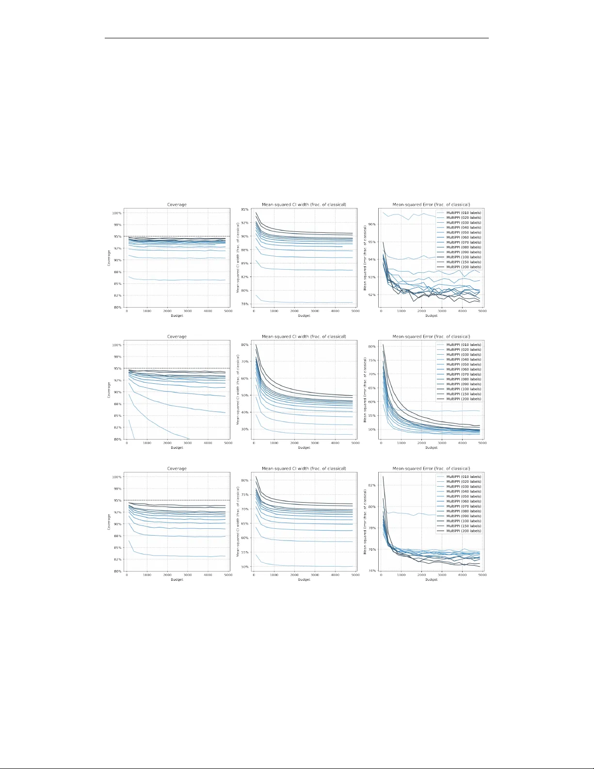
Published as a conference paper at ICLR 2026 M U L T I P L E - P R E D I C T I O N - P O W E R E D I N F E R E N C E Charlie Cowen-Br een 1 † Alekh Agarwal 2 Stephen Bates 1 William W . Cohen 3 Jacob Eisenstein 3 Amir Globerson 2 Adam Fisch 3 1 Massachusetts Institute of T echnology , 2 Google Research, 3 Google DeepMind † W ork done during internship at Google DeepMind. ccbreen@mit.edu , fisch@google.com . A B S T R AC T Statistical estimation often in volv es tradeoffs between expensi ve, high-quality measurements and a v ariety of lower -quality proxies. W e introduce Multiple- Prediction-Powered Inference (MultiPPI): a general framew ork for constructing statistically ef ﬁcient estimates by optimally allocating resources across these div erse data sources. This work provides theoretical guarantees about the minimax optimality , ﬁnite-sample performance, and asymptotic normality of the MultiPPI estimator . Through experiments across three div erse lar ge language model (LLM) ev aluation scenarios, we show that MultiPPI consistently achieves lower estimation error than existing baselines. This advantage stems from its budget-adapti ve allocation strategy , which strategically combines subsets of models by learning their complex cost and correlation structures. 1 I N T RO D U C T I O N Efﬁciently estimating expectations of random v ariables under a ﬁxed b udget is a fundamental prob- lem in many scientiﬁc settings. This paper addresses the general problem of optimally estimating such expectations when each random v ariable has an associated sampling cost, subject to a ﬁxed total budget constraint. W e are speciﬁcally motiv ated by the challenge presented by AI model ev aluation, which is a critical, but often resource-intensi ve, step in model dev elopment and maintenance. More concretely , in the AI model ev aluation setting, a variable X 1 might represent a high-quality but expensiv e metric computed for every model response to an input query , such as a score from a human annotator or a po werful proprietary model used as an "autorater". The remaining variables, X 2 , . . . , X k , might represent cheaper ev aluation options (e.g., scores from smaller autoraters or rule-based systems), which can be viewed as cov ariates or proxies for the true score. Gi ven the op- tion to obtain samples of X 1 , . . . , X k (either jointly or independently), the primary objectiv e is often to then estimate the mean of the high-quality score, E [ X 1 ] . In other cases, we may be interested in the mean difference between two scores, say , E [ X 1 − X 2 ] . The core dif ﬁculty in each case is in determining which of these variables to query , how many times to query them, and then ﬁnally how to combine them together to produce a statistically ef ﬁcient, consistent estimate of the ground truth. T o formalize this, let X := ( X 1 , . . . , X k ) be a set of random variables with ﬁnite v ariance. W e then consider the general problem of efﬁciently estimating any linear function of the mean of X subject to a total observ ation budget B . That is, for some a ∈ R k , we want to estimate θ ∗ = a ⊤ E [ X ] while spending no more than a total budget B on collecting subsets of joint random variables X I = { X i } i ∈ I at cost c I for index subsets I ⊆ { 1 , . . . , k } . More precisely , if n I is the number of times the subset X I is observed, we require that the n I satisfy a system of linear budget constraints of the form P I c I n I ≤ B , where the sum is over all such collected subsets I . Estimating linear functions of E [ X ] allo ws for ﬂe xibility in how θ ∗ is deﬁned. Given the AI e valua- tion setting abo ve, for example, measuring E [ X 1 ] corresponds to a = (1 , 0 , . . . , 0) , while measuring E [ X 1 − X 2 ] corresponds to a = (1 , − 1 , 0 , . . . , 0) . The ﬂexibility to observ e subsets of X also intro- duces a key trade-off that is unique with respect to previous related approaches to estimation. As we will show , observing variables jointly can be adv antageous by reducing overall estimation v ariance. 1 Published as a conference paper at ICLR 2026 This beneﬁt, howe ver , must be weighed against the data acquisition costs, c I . W e make no assump- tions about the structure of these costs (e.g., they may be non-additi ve over the components in I ). For instance, in our AI ev aluation setting, obtaining predictions from multiple autoraters can often be parallelized, so the cost of multiple predictions (in latency) is not signiﬁcantly more than that of the single slo west one. This is not always true; in medical diagnostics, for example, ordering many tests may become too taxing for a patient, and therefore undesireable or impossible to do jointly . T o solve this cost-optimal, multi-variate estimation problem, we introduce the Multiple-Prediction- Powered Inference (MultiPPI) estimator, which is a cost-aw are generalization of the Ef ﬁcient Prediction-Powered Inference (PPI++) estimator of Angelopoulos et al. ( 2023b ), and extends it to optimally le verage multiple types of predictions to power inference . The MultiPPI estimator constructs a lo w-variance, consistent estimate of θ ⋆ by combining observ ations from judiciously chosen subsets of X . The core of our method is an optimization procedure that jointly determines the number of samples n I to draw from each subset I and the corresponding linear weights λ I used to form the ﬁnal estimate. W e demonstrate that this allocation problem can be formulated as a second-order cone program (SOCP) for a single budget constraint, and a semideﬁnite program (SDP) for multiple budget constraints, and thus solv ed efﬁciently using standard techniques. Theoretically , we show that the MultiPPI estimator is minimax optimal when the joint cov ariance matrix, Σ = Co v ( X ) , is kno wn. For the typical case where it is unknown, ho wev er , we pro vide a frame work for integrating an initial estimation phase where an approximation of the required cov ariance matrix, b Σ , can be derived from either a small "burn-in" sample or a pre-existing labeled "transfer" dataset (a common scenario in applied settings)—and pro vide ﬁnite-sample bounds on the performance degradation that is incurred by substituting b Σ for Σ . Finally , we empirically demon- strate the ef fectiv eness of this approach across three div erse LLM ev aluation settings, including choosing between autoraters of different sizes, autoraters with different test-time reasoning con- ﬁgurations, and complex multi-autorater-debate scenarios. In all cases, our method achiev es lower mean-squared error and tighter conﬁdence interv als for a gi ven annotation budget than e xisting base- lines. W e demonstrate that MultiPPI achieves this by automatically tailoring its strategy to the av ail- able b udget B : that is, it learns to rely primarily on the cheaper autoraters when the budget is small, and naturally begins to incorporate more expensi ve, better autoraters as the b udget increases. T aken together , our work provides a principled and computationally tractable framew ork for cost-effecti ve, model-aided statistical inference, in settings with complex cost-v ersus-performance tradeoffs. In summary , our main contributions are as follo ws: • W e introduce the MultiPPI estimator and frame the problem of ﬁnding the optimal subset sam- pling strategy and estimator weights as an ef ﬁcient second-order cone program (SOCP). • W e prov e that the MultiPPI estimator is minimax optimal when the covariance matrix Σ of X 1 , . . . , X k is known, and provide ﬁnite-sample performance guarantees for the practical setting where the cov ariance matrix must ﬁrst be estimated as a part of the ov erall inference problem. • W e demonstrate MultiPPI’ s applicability across multiple LLM ev aluation settings, and show how it can effecti vely combine signals from different model sizes, reasoning conﬁgurations, and multi-agent debates to achiev e lower error and tighter conﬁdence inter vals for a giv en budget. 2 R E L AT E D W O R K Our work builds upon Prediction-Po wered Inference (PPI; Angelopoulos et al. , 2023a ), a statistical framew ork for efﬁciently estimating population-level quantities by augmenting a small set of labeled data with predictions from a machine learning (ML) model. W e speciﬁcally build on PPI++, the efﬁcient extension of PPI introduced in Angelopoulos et al. ( 2023b ), which also further improves variance by optimally re weighting these predictions. W e describe PPI in greater depth in Section 3 . PPI is part of a broader class of statistical methods that lev erage ML predictions for estimation. Its principles connect to classical control variates and difference estimators ( Ripley , 1987 ; Särndal et al. , 1992 ; Chaganty et al. , 2018 ), which reduce variance by subtracting a correlated random variable with a kno wn mean; the correlated v ariable in PPI is the ML prediction, whose mean can be (cheaply) estimated on unlabeled data. This approach also shares theoretical foundations with modern semi- parametric inference, particularly methods from the causal inference literature like Augmented In- 2 Published as a conference paper at ICLR 2026 verse Propensity W eighting (AIPW ; Robins & Rotnitzky , 1995 ), T argeted Maximum Lik elihood Es- timation (TMLE; v an der Laan & Rubin , 2006 ), and double machine learning (DML; Chernozhukov et al. , 2018 ). Recently , PPI has been applied to Generati ve AI e valuation, where human annotations (or more generally , annotations from some trusted source) are combined with cheaper "autorater" outputs for efﬁcient, unbiased estimates of model performance ( Boyeau et al. , 2024 ; Chatzi et al. , 2024 ; Fisch et al. , 2024 ; Angelopoulos et al. , 2025 ; Saad-Falcon et al. , 2024 ; Demirel et al. , 2024 ). Existing PPI frameworks, howe ver , assume either a single predictor ( Angelopoulos et al. , 2023a ; b ) or a ﬁxed set of predictors queried together ( Miao et al. , 2024 ). W e address the common scenario where multiple predictors (e.g., autoraters) with different cost-performance proﬁles are av ailable. This introduces a complex budget allocation problem: determining which predictors to query (in- dividually , jointly , or in any joint subset), ho w often to query them, and how to combine the mea- surements they provide for a minimum-variance estimate under a ﬁxed budget. Our work partially generalizes Angelopoulos et al. ( 2025 ), which optimizes a sampling polic y for a single predictor . Unlike that work, howe ver , which focuses on input-conditional policies and expected budget con- straints, we ﬁnd a ﬁxed allocation policy that al ways satisﬁes a hard b udget constraint for e very run. Our allocation problem is also related to budgeted regression with partially observ ed features ( Cesa- Bianchi et al. , 2011 ; Hazan & Koren , 2012 ) and acti ve learning or testing ( Settles , 2009 ; Kossen et al. , 2021 ; Zhang & Chaudhuri , 2015 ). W e emphasize, howe ver , that our goal is estimation of a linear function of a population mean (i.e., a ⊤ E [ X ] ), and not regression (e.g., predicting X 1 from X 2 , . . . , X k ). While related, standard approaches to re gression, including with partial observ ations, optimize for sample-wise predicti ve accuracy rather than for predictiv e accurac y of a population- lev el quantity . Our problem also connects to multi-armed bandit allocation for adaptive Monte Carlo estimation ( Neufeld et al. , 2014 ). A ke y difference is that these framew orks often use sequential, input-dependent policies to minimize regret, making it difﬁcult to deriv e valid conﬁdence intervals (CIs). Our framew ork, in contrast, computes a ﬁxed allocation policy ov er predictiv e models (not individual inputs as in activ e learning or testing) and guarantees unbiased estimates with valid CIs. Even more broadly , our work shares similar high-le vel goals with transfer learning and domain adaptation ( Pan & Y ang , 2010 ; Ben-Da vid et al. , 2010 , inter alia )—i.e., leveraging signals of varying quality and potential bias—though the statistical techniques are distinct. 3 P R E L I M I N A R I E S In the following section, we introduce the general estimation problem of interest and summarize existing approaches. Suppose that we are interested in the mean of a random variable X 1 , which is dependent upon another random variable X 2 (corresponding to estimating a ⊤ E [ X ] for a = (1 , 0) as described in § 1 ). For example, in the AI model ev aluation setting, X 2 may be an autorater’ s score for a model output to a user’ s query , and X 1 may be the ground truth quality of the response as measured by an expert human annotator . Suppose we have access to a small number ( n ) of i.i.d. samples that contain labels from both the target rater ( X 1 ) and autorater ( X 2 ), and a large number ( N ) of i.i.d. samples that contain only the autorater predictions ( ˜ X 2 ). A naïve approach to estimat- ing the mean is to simply take the sample a verage of X 1 and ignore X 2 entirely , which we denote by ˆ θ classic = 1 n P n j =1 X ( j ) 1 . When the prediction X 2 is correlated with X 1 and easy to query , ho wever , it is natural to consider the "prediction-powered" PPI estimator ( Angelopoulos et al. , 2023a ; b ): ˆ θ PPI = 1 n n X j =1  X ( j ) 1 − X ( j ) 2  + 1 N N X j =1 ˜ X ( j ) 2 (1) When we can afford to take N to be very large, it is clear that the variance of ˆ θ PPI is much smaller than that of ˆ θ classic provided that our model predictions X 2 are close to X 1 in mean-squared error . When that fails, Angelopoulos et al. ( 2023b ) propose adding a linear ﬁt of the form: ˆ θ PPI++ = 1 n n X j =1  X ( j ) 1 − λX ( j ) 2  + 1 N N X j =1 λ ˜ X ( j ) 2 . (2) The parameter λ may be chosen to minimize the variance of ˆ θ PPI ++ based on the observed labeled data. This strategy yields an estimator which asymptotically improv es on ˆ θ classic and ˆ θ PPI in the 3 Published as a conference paper at ICLR 2026 limit that n → ∞ and N ≫ n . T ow ard the setting where n and N may be comparable in size, if one is able to choose to or not to request a label X ( j ) 1 for e very observed unlabeled point X ( j ) 2 , a modiﬁcation of ˆ θ PPI++ allows one to do so in a cost-optimal w ay ( Angelopoulos et al. , 2025 ). 3 . 1 M U LT I P L E P R E D I C T I V E M O D E L S How should one adapt the preceding setting when one has access to many predictions, rather than just X 2 ? One option is to stack all predictions into a vector X 2: k := ( X 2 , . . . , X k ) and choose λ ∈ R k − 1 to be a vector in ˆ θ PPI++ ; this is the estimator proposed by Miao et al. ( 2024 ), and can be written ˆ θ PPI++ vector = 1 n n X j =1  X ( j ) 1 − λ ⊤ X 2: k  + 1 N N X j =1 λ ⊤ ˜ X ( j ) 2: k (3) But this approach is suboptimal when (as is becoming standard) the best models may be available only for the highest prices: if any of X 2 , . . . , X k is expensi ve to obtain, our ability to sample X 2: k will be limited. This yields suboptimal results, as we show in § 6 . One may instead decide to perform PPI with just one model X i , for whichever i  = 1 has the best cost/accuracy tradeof f—but it is not clear a priori which one this is, or ho w much worse it may be compared to some combination of a cost-ef fective subset of X . Alternativ ely , perhaps it is possible for cheaper models be used to recursiv ely estimate the means of more expensi ve models, thus creating a PPI++ cascade : for instance, if k = 3 and ( X 1 , X 2 , X 3 ) are in decreasing order of cost, we might consider ˆ θ PPI++ cascade = 1 n n X j =1  X ( j ) 1 − λX ( j ) 2  + 1 N N X j =1  λ ˜ X ( j ) 2 − λ ′ ˜ X ( j ) 3  + 1 M M X j =1 λ ′ ˜ ˜ X ( j ) 3 (4) Each of these strategies can be realized as possible instances of the MultiPPI estimator we propose in the next section. Rather than coarsely limiting ourselves to sampling X 2: k = ( X 2 , . . . , X k ) together , we allow the ﬂe xibility of sampling X I for generic index subsets I ⊆ { 1 , . . . , k } . 4 M U L T I P L E - P R E D I C T I O N - P O W E R E D I N F E R E N C E ( M U L T I P P I ) As Section 3.1 highlights, it is not obvious how to best allocate a budget across a di verse suite of predictiv e models, where each model has its own cost and performance tradeoffs. W e begin by deﬁning the class of permissible estimators: W e require that the number of times, n I , that X I is sampled satisﬁes a linear budget constraint, speciﬁed by a set of non-negati ve costs c I ≥ 0 and total budget B ≥ 0 , for each index subset I ⊆ { 1 , . . . , k } . 1 Deﬁnition 1. An estimator ˆ θ is budget-satisfying if it a measurable function of n I i.i.d. samples of X I , for each I ⊆ { 1 , . . . , k } , such that P I n I c I ≤ B . T o de velop a principled search for the best b udget-satisfying estimator , we be gin by asking a simple question under idealized conditions: Question 1. If the covariance matrix, Σ = Cov( X ) , is e xactly known, what is the minimax optimal, budg et-satisfying estimator of θ ∗ = a ⊤ µ with r espect to the mean-squar ed err or , E [( ˆ θ − θ ∗ ) 2 ] ? The answer to Question 1 will provide us with a set of allocations n I and a corresponding budget- satisying estimator ˆ θ MultiPPI which we will e valuate on the n I samples of X I , for each I . Once we hav e addressed this question, we address the case of unkno wn Σ by describing strategies depending on the empirical cov ariance matrix b Σ , which may be estimated from data. It turns out, perhaps surprisingly , that Question 1 reduces to the following tractable alternati ve: Question 2. If the covariance matrix, Σ = Cov( X ) , is exactly known, what is the minimum vari- ance, linear, unbiased b udget-satisfying estimator of θ ∗ = a ⊤ µ ? W e demonstrate the equiv alence of Question 1 and Question 2 in Theorem 2 . For now , the "oracle" assumption on kno wing the covariance matrix Σ allows us to isolate the resource allocation problem 1 In Section B , we extend the methodology to multiple b udget constraints. 4 Published as a conference paper at ICLR 2026 from the separate challenge of estimating ho w closely related ( X 1 , . . . , X k ) are to begin with, and to analyze what a good procedure for le veraging multiple predictiv e models under cost constraints should look like in theory . All proofs of our theoretical results are deferred to Appendix F . 4 . 1 M U LT I P P I ( Σ ) : A M I N I M A X O P T I M A L A L G O R I T H M Recalling notation from Section 1 , let X ∈ R k denote a random vector of ﬁnite second moment with distribution P . Let I ⊆ 2 { 1 ,...,k } denote a collection of index subsets which may be queried, and for any I ∈ I , let X I = { X i } i ∈ I be the corresponding subset of X . Next, let n = { n I } I ∈I , n I ∈ N be an allocation of sample sizes, where n I i.i.d. samples are drawn for each subset I , and let λ = { λ I } I ∈I , λ I ∈ R | I | deﬁne a corresponding set of weighting v ectors for each subset I . Finally , let ˆ θ ( n, λ ) denote the weighted sum of sample means from each non-empty subset, i.e., ˆ θ ( n, λ ) = X I : n I > 0 1 n I n I X j =1 λ ⊤ I X ( j ) I . (5) The MultiPPI estimator , ˆ θ MultiPPI , is then deﬁned as the optimal estimator in this class that minimizes the MSE subject to our unbiasedness ( U ) and budget ( B ) constraints: ˆ θ MultiPPI = argmin ˆ θ ( n,λ ) E   ˆ θ ( n, λ ) − θ ∗  2  s.t. U and B hold , (6) where the constraints U and B are U ⇐ ⇒ E [ ˆ θ ( n, λ )] = θ ∗ for all P of ﬁnite second moment and B ⇐ ⇒ X I n I c I ≤ B . It can be shown that U reduces to a linear constraint on λ , which makes our optimization con venient. As previously discussed, the estimators of Equation ( 3 ) and Equation ( 4 ) can be viewed as special cases of this setup. F or instance, Equation ( 3 ) corresponds to imposing the additional restriction that λ I = 0 for all I ∈ 2 { 1 ,...,k } except for I = { 1 , . . . , k } and I = { 2 , . . . , k } ; Equation ( 4 ) corresponds to the additional restriction that λ I = 0 for all I except for { 1 , 2 } , { 2 , 3 } and { 3 } . 4 . 1 . 1 O P T I M I Z ATI O N Solving Equation ( 6 ) is, in general, non-tri vial. Since ˆ θ ( n, λ ) is linear in X , it can be sho wn that the optimal ( n, λ ) depend only on the covariance matrix Σ of X , and so we will denote by ˆ θ MultiPPI(Σ) the solution to Equation ( 6 ) given any distribution such that Σ = Cov( X ) . Then, it can be further shown (this follo ws from Theorem 2 , presented next) that the MSE of ˆ θ MultiPPI(Σ) is V B = min n : B holds supp( a ) ⊆ S { I : n I > 0 } a ⊤ S ( n ) a, S ( n ) = X I ∈I n I Σ † I ! † (7) where Σ I denotes the principle submatrix of Σ on I , embedded back into R k × k , and † denotes the Moore-Penrose pseudo-in verse. 2 The minimizing n of the above expression then also determines the optimal λ I to be the restriction of n I Σ † I S ( n ) a to the coordinates I . If the integrality constraints on n I are relaxed, we show in the appendix that this reduces to a second-order cone problem in the case of a single budget constraint, and a semi-deﬁnite program in the case of multiple b udget constraints. This allows for Equation ( 7 ) to be solv ed efﬁciently using standard techniques (Section G ). 4 . 1 . 2 M I N I M A X O P T I M A L I T Y The minimal MSE V B shown in Equation ( 7 ) has a more fundamental characterization. Here we show that it is in fact the minimax optimal MSE achiev able by any budget-satisfying estimator , taken 2 More formally , if P I ∈ R k × k denotes the orthogonal projection onto span ( I ) ⊆ R k , we deﬁne Σ I = P I Σ P ⊤ I , and so Σ † I := ( P I Σ P ⊤ I ) † . 5 Published as a conference paper at ICLR 2026 ov er the set of distrib utions P of covariance Σ . Consequently , the estimator deﬁned by ˆ θ MultiPPI (Σ) is minimax optimal ov er the set of distributions P Σ = { distribution P on R k : Cov( X ) = Σ for X ∼ P } . Speciﬁcally , gi ven costs ( c I ) I and a budget B , let Θ B denote the set of budget-satisfying estimators ˆ θ per Theorem 1 . W e emphasize that we make no restriction on Θ B to include only linear or unbiased estimators. Then the follo wing result holds: Theorem 2 (Minimax optimality of MultiPPI for kno wn Σ ) . F or all Σ ≻ 0 , we have inf ˆ θ ∈ Θ B sup P ∈P Σ E h ( ˆ θ − θ ∗ ) 2 i = V ar  ˆ θ MultiPPI(Σ)  = V B , wher e the variance is with r espect to any distribution P ∈ P Σ . 4 . 2 M U LT I P P I ( b Σ ) : A P R A C T I C A L A L G O R I T H M In practice, Σ is rarely known and must be approximated by an estimated cov ariance matrix b Σ . In general, there are many methods for constructing an estimate b Σ of Σ , and many of the theoretical properties of MultiPPI are agnostic to the particular choice made. The follo wing theorem shows that, for any b Σ which con ver ges in probability to Σ as our b udget tends to inﬁnity , the MultiPPI estimator is asymptotically normal and achiev es the optimal v ariance of Theorem 2 . For this result, we need a technical condition which amounts to Equation ( 6 ) having a unique minimizer n as B → ∞ ; we state it formally in Section F .2 . Theorem 3. Suppose X ∈ R k has ﬁnite second moment, and suppose that Σ = Cov( X ) satisﬁes condition 14 . Suppose that b Σ p → Σ in the operator norm as B → ∞ . Then for ˆ θ MultiPPI( b Σ) arbitrarily dependent on any potential samples used to estimate b Σ , we have √ B  ˆ θ MultiPPI( b Σ) − θ ∗  d → N (0 , V ∗ ) as B → ∞ , wher e V ∗ = lim B →∞ B V B , and V B is deﬁned in Equation ( 7 ) . It is important to note that the estimator ˆ θ MultiPPI( b Σ) continues to enjoy unbiasedness, b udget satis- faction, and asymptotic normality reg ardless of mis-speciﬁcation in b Σ . A natural question concerns the le vel of suboptimality of ˆ θ MultiPPI( b Σ) as a function of the de gree of mis-speciﬁcation of b Σ in ﬁnite samples. Belo w , we present a meta-result which serves to quantify the sensitivity of our procedure to errors in the speciﬁcation of b Σ . Theorem 4 (Stability of MultiPPI) . Let P be a distribution of covariance Σ , and suppose that Σ has minimum eigen value γ min . Let σ 2 classical denote the least MSE of any b udget-satisfying sample mean of θ ∗ . Let b Σ denote any non-random symmetric positive-deﬁnite matrix. Then we have E   ˆ θ MultiPPI( b Σ) − θ ∗  2  ≤ V B + 4 σ 2 classical γ min ∥ b Σ − Σ ∥ F . whenever ∥ b Σ − Σ ∥ F ≤ γ min / 2 , wher e ∥ · ∥ F denotes the F r obenius norm. In general, there are many methods for constructing an estimate b Σ of Σ , and Theorem 4 is agnostic to the particular choice made. In Section E.1 , we sho w ho w to apply the meta-result abov e to deri ve a family of ﬁnite-sample bounds in a variety of distrib utional settings and for a variety of estimates b Σ . In practice, we estimate Σ from data, and ﬁnd the Ledoit-W olf estimator b Σ of the co variance matrix Σ to perform best in our experiments. This is consistent with the fact that the Ledoit-W olf estimate is designed to minimize E ∥ b Σ − Σ ∥ F , and Theorem 4 shows that the error of ˆ θ MultiPPI( b Σ) is controlled by ∥ b Σ − Σ ∥ F . In Theorem 9 , we apply Theorem 4 to provide ﬁnite-sample performance guarantees on MultiPPI when the Ledoit-W olf estimator is used to estimate cov ariance. In our experiments, we ev aluate ˆ θ n,λ on the same samples we used to estimate b Σ . A similar approach was taken by Angelopoulos et al. ( 2023b ) for PPI++ when tuning the value of λ , and we ﬁnd that it is easy to implement and yields strong empirical results in practice. 6 Published as a conference paper at ICLR 2026 Note that while the data reuse introduces bias in ﬁnite samples—due in part to the additional dependency of λ I on X I in Equation ( 5 )—it preserves consistency and asymptotic normality in the limit as our b udget B and the number of (reused) b urn-in samples tend to inﬁnity . For an analysis of the bias introduced in ﬁnite samples, see Section E.5 . 4 . 2 . 1 P RO C E D U R E W e no w specify an easy-to-implement procedure that makes use of a b urn-in of N fully labeled samples to est imate b Σ , and then also reuses the N samples when estimating ˆ θ MultiPPI ( b Σ) . Speciﬁcally , we target the practical setting where we are giv en N fully-labeled samples a priori , and ha ve no ability to obtain more. This is typical of real-world settings in which we are given, or hav e already collected, a ﬁxed dataset of "gold" labels that we are then trying to augment with PPI related techniques—and may be encapsulated by the budget constraint n { 1 ,...,k } ≤ N . While we may not be able to obtain more fully-labeled samples, we may be afforded a separate computational budget for querying model predictions that then augment the N fully-labeled samples; taken together , this setting is represented by a system of budget constraints. 3 In summary , we propose the following: 1. Estimate the co variance matrix b Σ on the N fully-labeled samples, which we will reuse in Step 3. 2. Solve for the n I , λ I which minimize Equation ( 6 ) gi ven b Σ . W e refer to this as MultiAllocate ( b Σ) . 3. Sample the n I , ∀ I ∈ I additional data points accordingly , and return ˆ θ MultiPPI ( b Σ) , ev aluated on both the n I additional data points for each I ∈ I , and the N (reused) initial samples. 5 E X P E R I M E N TA L S E T U P In each experiment, our goal is to estimate the mean θ ∗ = E [ X 1 ] of some random variable X 1 to be speciﬁed, which we will refer to as the targ et . This corresponds to the choice a = (1 , 0 , . . . , 0) in our notation. W e will also specify a model family ( X 2 , . . . , X k ) , together with a cost structur e ( c I ) I ∈I . In each experiment, we are given some number of samples for which the entire v ector X = ( X 1 , . . . , X k ) is visible; we refer to such samples as fully-labeled . Giv en these samples, we perform the procedure outlined in Section 4.2.1 : we estimate b Σ using these samples, sample from the auxiliary models ( X 2 , . . . , X k ) according to the allocation speciﬁed by MultiAllocate ( b Σ) , and return ˆ θ MultiPPI( b Σ) , e valuated on both the N fully-labeled samples and the additional auxiliary data. Baselines: In each experiment, we compare to se veral baselines. First, we compare to classical sampling. Second, we compare to PPI++ with each model included in the family (speciﬁed in Equation ( 2 )), and to vector PPI++ with e very model in the family (speciﬁed in Equation ( 3 )). Experiment 1: Estimating Arena win-rates by autorater ensembles. W e focus on the Chatbot Arena dataset ( Chiang et al. , 2024 ), where of interest is the win-rate between a pair of models, which is the probability that a giv en user prefers the response of one model to that of the other . The randomness is taken over the prompt, the user, and the model responses. Here, we aim to estimate the win-rate between Claude-2.1 and GPT -4-1106-Previe w; this is our targ et . Our model family consists of autoraters built on Gemini 2.5 Pro (without thinking) and Gemini 2.5 Flash. In our notation, we hav e ( X 1 , X 2 , X 3 ) = ( human label , Gemini 2.5 Pro label , Gemini 2.5 Flash label ) . W e draw model costs from the Gemini developer API pricing guide ( Gemini API ), see Section I . In this case, the cost of querying both models is simply the sum of the costs of querying each model independently . Experiment 2: Optimal test-time autorater scaling on ProcessBench. In this experiment, we aim to estimate the fraction of correct solutions in the ProcessBench dataset ( Zheng et al. , 2024 ), giv en a small number of labeled examples. The task is simpliﬁed from its original form to a binary classiﬁcation problem: determining whether a gi ven math proof solution contains a process error , without identifying the speciﬁc step. W e employ Gemini 2.5 Pro with a v ariable thinking budget as our autorater . Its accuracy correlates with the number of words e xpended in the thought, with performance gains saturating after approximately 500 words (see Figure 12 in the appendix). W e create a family of four autoraters by checkpointing the model’ s thought process at 125, 250, 375, 3 W e explain ho w to solve the optimization problem posed by such systems in Appendix B . 7 Published as a conference paper at ICLR 2026 and 500 w ords. A key aspect of this setup is the non-additi ve, cascading cost structure. Generating a response from a model with a larger thinking budget makes the outputs of all smaller-b udget models av ailable at a marginal cost. Consequently , the total cost for a subset of models S is modeled with two components: an input cost proportional to the sum of the word budgets in S, and an output cost proportional to the maximum word b udget in S. Explicitly , for S ⊆ { 125 , 250 , 375 , 500 } , we set c S = output_cost_per_word · max S + input_cost_per_word · X S (8) For concision, in our results we refer to the model assessments after 125, 250, 375, and 500 words by “tiny , ” “small, ” “medium, ” and “lar ge, ” respectively . Experiment 3: Hybrid factuality evaluation through multi-autorater debate. Following Du et al. ( 2023 ), we ev aluate the factual consistency of biographies for 524 computer scientists gener- ated by Gemini 2.5 Pro. For each person p ∈ P , we compare their Gemini-generated biography b p against a set of kno wn grounding facts F p = { f p 1 , . . . , f p m p } about the person. Our target metric is the proportion of factually consistent pairs ( b, f ) within the total set S = { ( b p , f p ) : p ∈ P , f p ∈ F p } . Concretely , we tar get the proportion |{ ( b, f ) ∈ S : ( b, f ) is factually consistent }| / |S | . Ground-truth consistenc y of a pair ( b, f ) is established by majority v oting ov er ﬁ ve independent judgments from Gemini 2.5 Pro with thinking, a method validated by Du et al. ( 2023 ) to hav e ov er 95% agreement with human annotators. Our experiment, illustrated in Figure 13 , assesses the performance of a more cost-effecti ve model, Gemini 2.0 Flash Lite, as an autorater . T o elicit better autoratings from queries to Gemini 2.0 Flash Lite, we bootstrap performance via multi-round debate. For a ﬁxed number of agents A ∈ { 1 , 2 , 3 } , and a ﬁxed number of maximum rounds R ∈ { 1 , 2 } , we perform the following procedure: In each round, A instances of Flash Lite are independently prompted to provide a reasoned judgment on the consistency of a pair ( b, f ) ∈ S . A "pooler" instance of Flash Lite then consolidates these responses into a single yes , no , or uncertain output. A deﬁnitive yes or no concludes the process. If the pooler outputs uncertain , and the number of maximum rounds R has not yet been reached, the A agents re view all prior responses and continue their debate in a new round. If the output remains uncertain after the ﬁnal round, either yes or no is reported with equal probability—since the dataset is balanced, this outcome is fair insofar as it is as good as random guessing. W e impose the maximum round restriction to encapsulate our budget constraint. For a gi ven ( A, R ) , the cost is A · R ; for collections, the cost follows Equation ( 8 ). 6 E M P I R I C A L R E S U L T S W e plot MultiPPI, and the baselines described in Section 5 , for a b udgets between 0 and 2 k units of cost. W e normalize model costs so that one unit of cost always represents exactly one query to our most expensiv e model. For each ﬁxed budget and each method, we estimate the target, and construct asymptotic 95% conﬁdence interv als C based on Theorem 3 . W e plot (i) cov erage, P ( θ ∗ ∈ C ) ; (ii) conﬁdence interval width, |C | ; and (iii) mean-squared error E [( ˆ θ − θ ∗ ) 2 ] . W e report both the conﬁdence interv al width and the mean-squared error as a fraction of what classical sampling achiev es (lower is better). In each case, the target is θ ∗ = E [ X 1 ] , and P and E are computed with respect to the empirical distribution over the dataset observed (we perform 500 k random trials with 250 gi ven labels). Note that these 250 labeled points are evidently enough for all estimators considered to achiev e good coverage (in Section D.2 we also include results with 1 k labeled points). W e implement the optimization scheme in cvxpy , and use CVXOPT as our choice of optimizer . Experiment 1: Chatbot Arena. Results are shown in Figure 1 (top). Observe that different base- lines dominate in different budget re gimes. In the lo w-budget regime, scalar PPI++ with Gemini 2.5 Flash is the best baseline, while in the large-b udget regime, vector PPI++ with both Gemini 2.5 Pro and Gemini 2.5 Flash is the best baseline. Howe ver , we see that MultiPPI improves on all baselines in all regimes. In the appendix, Figure 5 and Figure 2 plot the λ I and n I values learned by MultiPPI across budget regimes. Note that the learned values tend to the speciﬁcations for PPI++ with Gemini 2.5 Flash in the low-b udget regime, and to the speciﬁcations for vector PPI++ in the large-b udget regime, a ﬁnding that we rigorously pro ve happens in broader generality in Section E.2 . Lastly , note that PPI++ with Gemini 2.5 Pro is suboptimal in all regimes. In other words, PPI++ with Gemini 2.5 Pro is not included in the Pareto frontier . This is because, for this task, its correlation with the label is no more than that of PPI++ with Gemini 2.5 Flash, yet it is strictly more expensi ve. 8 Published as a conference paper at ICLR 2026 Experiment 2: ProcessBench. Results are shown in Figure 1 (middle). Again, we see that each baseline has a range of budgets for which it outperforms all other baselines. In particular , the cheaper models yield better performance when used in PPI++ in the smaller-b udget regimes, while the more-e xpensiv e models yield better performance in the higher-b udget regimes. In particular , vector PPI++, which uses all k − 1 models, steadily improv es as the budget increases, but only outperforms the other baselines at the highest budgets. This behavior is explained by Figure 12 in the appendix, which sho ws that predictive performance improves for larger thinking budgets. Thus the more expensi ve models yield higher correlation with the label and thus yield low-v ariance rec- tiﬁers; on the other hand, their high cost means that this decrease in rectiﬁer v ariance is outweighed by our inability to draw an adequate number of samples from them in the lo w-budget re gimes. Of note is the fact that the models which think for longer are not in general less biased . This phenomenon is shown in Figure 15 , which shows that thinking for longer is not enough to resolve the systematic bias present in the autorater . Howe ver , the ﬁgure also shows that simple debiasing schemes like PPI resolve this issue. Note that this trend is not reﬂected in the correlations between these models and the label, because correlation is in variant to addition of constants. Finally , MultiPPI improv es on all baselines methods in all regimes. Interestingly , Figure 3 and Figure 4 show that the parameters λ I and n I learned by MultiPPI transition from emulating PPI++ with the tiny model (which is the best baseline in the low-b udget regime) to emulating a cascaded version of PPI (see Equation ( 4 )), in which the medium model is used to debias the larger model. Experiment 3: Biography factuality evaluation. Results are shown in Figure 1 (bottom). Once again, each baseline is dominant over the others in certain regimes; MultiPPI improv es on all base- lines in all regimes. Of note, howe ver , is the fact that the coverage of all estimators considered, but MultiPPI and vector PPI++ in particular , degrades slightly in the large-b udget regime (i.e., the 95% CI under-cov ers by ≈ 1%) . W e discuss this interesting phenomenon in Section E.5 , and ﬁnd that it does not occur when the number of labeled samples gro ws in constant proportion with the budget (see, for example, our additional results with N = 1000 fully-labeled samples in Section D.2 ). In terms of the performance-vs-cost proﬁle that MultiPPI leverages: Figure 13 shows that predictiv e performance increases, across many metrics, as the number of agents and number of rounds in- creases. Note, ho wev er , that a marginal increase in number of agents yields a greater increase in ac- curacy than a mar ginal increase in number of rounds (this is largely because the pooler is more likely to report "uncertain" after the end of the ﬁrst round than after the end of the second; see Figure 14 ). 7 C O N C L U S I O N In this work, we introduce Multiple-Prediction-Powered Inference (MultiPPI), a frame work for efﬁ- ciently estimating expectations under budget constraints by optimally lev eraging multiple informa- tion sources of v arying costs. MultiPPI formulates the optimal allocation of queries across subsets of variables as a second-order cone program in the case of a single budget constraints, or a semi-deﬁnite program in the case of multiple—both can be efﬁcienc y solved using of f-the-shelf tools. W e provide theoretical guarantees, including minimax optimality when co variances are kno wn, and demonstrate empirically across diverse LLM ev aluation tasks that MultiPPI outperforms existing methods. By adaptiv ely balancing cost and information, MultiPPI achie ves lower error for a given budget, au- tomatically shifting its strategy from cheaper proxies to more expensi ve, accurate predictors as the budget increases, thus of fering a principled and practical solution for cost-effectiv e inference. 9 Published as a conference paper at ICLR 2026 Experiment 1: Chatbot Arena 0 2 , 000 4 , 000 90 % 92 % 94 % 96 % 98 % 100 % Budget Coverage 0 2 , 000 4 , 000 92 % 94 % 96 % Budget Mean-squared CI width (frac. of classical) 0 2 , 000 4 , 000 92 % 94 % 96 % Budget Mean-squared Error (frac. of classical) MultiPPI PPI++ V ector PPI++ Scalar (Pro) PPI++ Scalar (Flash) Experiment 2: ProcessBench 0 2 , 000 4 , 000 90 % 92 % 94 % 96 % 98 % 100 % Budget Coverage 0 2 , 000 4 , 000 50 % 60 % 70 % 80 % Budget Mean-squared CI width (frac. of classical) 0 2 , 000 4 , 000 50 % 60 % 70 % 80 % Budget Mean-squared Error (frac. of classical) PPI++ Scalar Large PPI++ Scalar Medium PPI++ Scalar Small PPI++ Scalar Tiny MultiPPI PPI++ V ector Experiment 3: Factuality 0 2 , 000 4 , 000 90 % 92 % 94 % 96 % 98 % 100 % Budget Coverage 0 2 , 000 4 , 000 75 % 80 % 85 % 90 % Budget Mean-squared CI width (frac. of classical) 0 2 , 000 4 , 000 75 % 80 % 85 % 90 % Budget Mean-squared Error (frac. of classical) MultiPPI PPI++ V ector PPI++ Scalar 1 agent, 1 round PPI++ Scalar 2 agents, 1 round PPI++ Scalar 3 agents, 1 round PPI++ Scalar 1 agent, 2 rounds PPI++ Scalar 2 agents, 2 rounds PPI++ Scalar 3 agents, 2 rounds Figure 1: Results by budget for the experiments on Chatbot Arena (a), ProcessBench (b), and Fac- tuality (c). F or each estimator (all baselines and MultiPPI), the left column plots the empirical cov- erage of the 95% CI, the middle column plots the width of the 95% CI, and the right column plots the empirical mean-squared error of the point estimate. The fully-labeled sample size N is 250. A C K N O W L E D G E M E N T S W e are very grateful for insightful comments and suggestions by the anonymous re viewers. W e are also grateful for helpful discussions with Jonathan Berant, Michael Beukman, Frederic Jørgensen, Petros Karypis, Chris Dyer , and Martin W ainwright. R E P R O D U C I B I L I T Y S TA T E M E N T T o ensure reproducibility , we provide a detailed speciﬁcation of the algorithm in Section C . W e also include implementation details in Section I , and address computational considerations in Section G . Finally , all experiments sho wn in § 6 were av eraged over 500k trials. R E F E R E N C E S Anastasios N Angelopoulos, Stephen Bates, Clara Fannjiang, Michael I Jordan, and Tijana Zrnic. Prediction-powered inference. Science , 382(6671):669–674, 2023a. 10 Published as a conference paper at ICLR 2026 Anastasios N Angelopoulos, John C Duchi, and T ijana Zrnic. PPI++: Ef ﬁcient prediction-powered inference. arXiv pr eprint arXiv:2311.01453 , 2023b. Anastasios N. Angelopoulos, Jacob Eisenstein, Jonathan Berant, Alekh Agarwal, and Adam Fisch. Cost-optimal activ e ai model e valuation. arXiv pr eprint arXiv 2506.07949 , 2025. URL https: //arxiv.org/abs/2506.07949 . Shai Ben-David, John Blitzer , K oby Crammer, Alex K ulesza, Fernando Pereira, and Jennifer W ort- man V aughan. A theory of learning from different domains. Mach. Learn. , 79(1–2):151–175, May 2010. doi: 10.1007/s10994- 009- 5152- 4. URL https://doi.org/10.1007/ s10994- 009- 5152- 4 . Stephen Boyd and Lie ven V andenberghe. Conve x optimization . Cambridge uni versity press, 2004. Pierre Boyeau, Anastasios N Angelopoulos, Nir Y osef, Jitendra Malik, and Michael I Jordan. Au- toEval done right: Using synthetic data for model ev aluation. arXiv pr eprint arXiv:2403.07008 , 2024. Nicoló Cesa-Bianchi, Shai Shalev-Shwartz, and Ohad Shamir . Efﬁcient learning with partially observed attributes. J ournal of Machine Learning Resear ch , 12(87):2857–2878, 2011. URL http://jmlr.org/papers/v12/cesa- bianchi11a.html . Arun Chaganty , Stephen Mussmann, and Percy Liang. The price of debiasing automatic metrics in natural language ev alaution. In Iryna Gurevych and Y usuke Miyao (eds.), Pr oceedings of the 56th Annual Meeting of the Association for Computational Linguistics (V olume 1: Long P apers) , pp. 643–653, Melbourne, Australia, July 2018. Association for Computational Linguistics. doi: 10.18653/v1/P18- 1060. URL https://aclanthology.org/P18- 1060/ . Ivi Chatzi, Eleni Straitouri, Suhas Thejaswi, and Manuel Gomez Rodriguez. Prediction- powered ranking of large language models. In A. Globerson, L. Mackey , D. Bel- grav e, A. Fan, U. Paquet, J. T omczak, and C. Zhang (eds.), Advances in Neural In- formation Pr ocessing Systems , volume 37, pp. 113096–113133. Curran Associates, Inc., 2024. URL https://proceedings.neurips.cc/paper_files/paper/2024/ file/cd47cd67caa87f5b1944e00f6781598f- Paper- Conference.pdf . V ictor Chernozhukov , Denis Chetveriko v , Mert Demirer, Esther Duﬂo, Christian Hansen, Whitney Newe y , and James Robins. Double/debiased machine learning for treatment and structural pa- rameters. The Econometrics Journal , 21(1):C1–C68, 01 2018. URL https://doi.org/10. 1111/ectj.12097 . W ei-Lin Chiang, Lianmin Zheng, Y ing Sheng, Anastasios Nikolas Angelopoulos, T ianle Li, Dacheng Li, Banghua Zhu, Hao Zhang, Michael Jordan, Joseph E Gonzalez, et al. Chatbot arena: An open platform for ev aluating llms by human preference. In F orty-ﬁrst International Confer ence on Machine Learning , 2024. Ilker Demirel, Ahmed Alaa, Anthony Philippakis, and David Sontag. Prediction-powered general- ization of causal inferences. arXiv pr eprint arXiv:2406.02873 , 2024. Y ilun Du, Shuang Li, Antonio T orralba, Joshua B T enenbaum, and Igor Mordatch. Improving fac- tuality and reasoning in language models through multiagent debate. In F orty-ﬁrst International Confer ence on Machine Learning , 2023. Adam Fisch, Joshua Maynez, R. Alex Hofer , Bhuw an Dhingra, Amir Globerson, and W illiam W . Cohen. Stratiﬁed prediction-powered inference for ef fectiv e hybrid ev aluation of language mod- els. In The Thirty-eighth Annual Confer ence on Neural Information Pr ocessing Systems , 2024. URL https://openreview.net/forum?id=8CBcdDQFDQ . Gemini API. Gemini Developer API Pricing | Gemini API. URL https://ai.google.dev/ gemini- api/docs/pricing . Elad Hazan and T omer K oren. Linear regression with limited observation. In ICML , 2012. Roger A Horn and Charles R Johnson. Matrix analysis . Cambridge uni versity press, 2012. 11 Published as a conference paper at ICLR 2026 Jannik K ossen, Sebastian Farquhar , Y arin Gal, and T om Rainforth. Acti ve testing: Sample-efﬁcient model ev aluation. In ICML , 2021. URL http://dblp.uni- trier.de/db/conf/icml/ icml2021.html#KossenFGR21 . Jiacheng Miao, Xinran Miao, Y ixuan W u, Jiwei Zhao, and Qiongshi Lu. Assumption-lean and data-adaptiv e post-prediction inference. arXiv pr eprint arXiv 2311.14220 , 2024. URL https: //arxiv.org/abs/2311.14220 . James Neufeld, Andras Gyorgy , Csaba Szepesv ari, and Dale Schuurmans. Adapti ve monte carlo via bandit allocation. In Eric P . Xing and T ony Jebara (eds.), Pr oceedings of the 31st International Confer ence on Machine Learning , volume 32 of Pr oceedings of Machine Learning Resear ch , pp. 1944–1952, Bejing, China, 22–24 Jun 2014. PMLR. URL https://proceedings.mlr. press/v32/neufeld14.html . Sinno Jialin Pan and Qiang Y ang. A surve y on transfer learning. IEEE T ransactions on Knowledge and Data Engineering , 22:1345–1359, 2010. URL https://api.semanticscholar. org/CorpusID:740063 . B. D. Ripley . Stochastic simulation . John Wile y & Sons, Inc., New Y ork, NY , USA, 1987. ISBN 0-471-81884-4. James M. Robins and Andrea Rotnitzk y . Semiparametric efﬁcienc y in multiv ariate regression mod- els with missing data. Journal of the American Statistical Association , 90(429):122–129, 1995. ISSN 01621459. URL http://www.jstor.org/stable/2291135 . Jon Saad-Falcon, Omar Khattab, Christopher Potts, and Matei Zaharia. ARES: An automated ev al- uation frame work for retriev al-augmented generation systems. In Ke vin Duh, Helena Gomez, and Ste ven Bethard (eds.), Pr oceedings of the 2024 Conference of the North American Chapter of the Association for Computational Linguistics: Human Language T echnologies (V olume 1: Long P apers) , pp. 338–354, Mexico City , Mexico, June 2024. Association for Computational Linguis- tics. doi: 10.18653/v1/2024.naacl- long.20. URL https://aclanthology.org/2024. naacl- long.20/ . Burr Settles. Active learning literature survey . Computer Sciences T echnical Report 1648, Uni- versity of W isconsin–Madison, 2009. URL http://axon.cs.byu.edu/~martinez/ classes/778/Papers/settles.activelearning.pdf . Carl-Erik Särndal, Bengt Swensson, and Jan Wretman. Model assisted survey sampling. Springer Series in Statistics , 1992. Mark J. van der Laan and Daniel Rubin. T ar geted maximum likelihood learning. The Inter - national J ournal of Biostatistics , 2(1), 2006. doi: 10.2202/1557- 4679.1008. URL https: //www.degruyter.com/document/doi/10.2202/1557- 4679.1008/html . Roman V ershynin. High-dimensional pr obability: An intr oduction with applications in data science , volume 47. Cambridge university press, 2018. Martin J W ainwright. High-dimensional statistics: A non-asymptotic viewpoint , volume 48. Cam- bridge univ ersity press, 2019. Chicheng Zhang and Kamalika Chaudhuri. Activ e learning from weak and strong labelers. In Advances in Neural Information Pr ocessing Systems , 2015. Chujie Zheng, Zhenru Zhang, Beichen Zhang, Runji Lin, Keming Lu, Bowen Y u, Dayiheng Liu, Jingren Zhou, and Junyang Lin. Processbench: Identifying process errors in mathematical rea- soning. arXiv pr eprint arXiv:2412.06559 , 2024. 12 Published as a conference paper at ICLR 2026 C O N T E N T S A Ethics statement 15 B Generalization to multiple budget inequalities 15 C Detailed speciﬁcation of the algorithm 15 C.1 The case of a single budget inequality , known Σ . . . . . . . . . . . . . . . . . . . 15 C.2 The case of multiple budget inequalities, kno wn Σ . . . . . . . . . . . . . . . . . . 16 C.3 The case of unknown Σ . . . . . . . . . . . . . . . . . . . . . . . . . . . . . . . . 17 D Additional experiments 18 D.1 Learned allocations and linear parameters . . . . . . . . . . . . . . . . . . . . . . 18 D.2 MultiPPI by varying number of labeled samples . . . . . . . . . . . . . . . . . . . 19 D.3 The impact of shrinkage covariance estimation . . . . . . . . . . . . . . . . . . . 19 D.4 Scalability and computational tractability of the estimator . . . . . . . . . . . . . . 19 D.5 Autorater accuracy scaling . . . . . . . . . . . . . . . . . . . . . . . . . . . . . . 19 E Additional theoretical results 27 E.1 Finite-sample bounds . . . . . . . . . . . . . . . . . . . . . . . . . . . . . . . . . 27 E.2 Behavior of the estimator in the limiting regimes . . . . . . . . . . . . . . . . . . 28 E.3 Rounding in the large budget re gime . . . . . . . . . . . . . . . . . . . . . . . . . 28 E.4 The continuous problem and its properties . . . . . . . . . . . . . . . . . . . . . . 29 E.5 Decay of coverage in the lar ge budget re gime . . . . . . . . . . . . . . . . . . . . 30 F Proofs 31 F .1 Proof of Theorem 2 . . . . . . . . . . . . . . . . . . . . . . . . . . . . . . . . . . 31 F .2 Proof of Theorem 3 . . . . . . . . . . . . . . . . . . . . . . . . . . . . . . . . . . 32 F .3 Proof of Theorem 4 . . . . . . . . . . . . . . . . . . . . . . . . . . . . . . . . . . 34 F .4 Proofs for Section E.1 . . . . . . . . . . . . . . . . . . . . . . . . . . . . . . . . . 34 F .4.1 Proof of Theorem 5 . . . . . . . . . . . . . . . . . . . . . . . . . . . . . . 34 F .4.2 Proof of Corollary 6 . . . . . . . . . . . . . . . . . . . . . . . . . . . . . 35 F .4.3 Proof of Corollary 7 . . . . . . . . . . . . . . . . . . . . . . . . . . . . . 35 F .4.4 Proof of Corollary 8 . . . . . . . . . . . . . . . . . . . . . . . . . . . . . 35 F .4.5 Proof of Theorem 9 . . . . . . . . . . . . . . . . . . . . . . . . . . . . . . 35 F .5 Proofs for Section E.2 . . . . . . . . . . . . . . . . . . . . . . . . . . . . . . . . . 36 F .5.1 Proof of Theorem 10 . . . . . . . . . . . . . . . . . . . . . . . . . . . . . 36 F .6 Proofs for Section E.4 . . . . . . . . . . . . . . . . . . . . . . . . . . . . . . . . . 38 F .6.1 Proof of Lemma 17 . . . . . . . . . . . . . . . . . . . . . . . . . . . . . 40 G Computational considerations 41 13 Published as a conference paper at ICLR 2026 H The dual pr oblem 42 I Experimental details 43 I.1 Generating model predictions . . . . . . . . . . . . . . . . . . . . . . . . . . . . . 43 I.1.1 Experiment 1: Chatbot Arena . . . . . . . . . . . . . . . . . . . . . . . . 43 I.1.2 Experiment 2: Processbench . . . . . . . . . . . . . . . . . . . . . . . . . 43 I.1.3 Experiment 3: Biography factuality . . . . . . . . . . . . . . . . . . . . . 44 I.2 Constructing the MultiPPI estimator . . . . . . . . . . . . . . . . . . . . . . . . . 45 14 Published as a conference paper at ICLR 2026 A E T H I C S S TA T E M E N T This paper describes fundamental research on techniques for constructing statistically ef ﬁcient esti- mates of a target metric by optimally allocating resources across multiple types of proxy measure- ments. The primary intended use case which is analyzed in this work is the e valuation of generati ve AI systems, for which reliable ev aluation is a core technical challenge. Efﬁcient and precise esti- mates of model performance can help make AI systems easier to build, deploy , and monitor . W e do not speculate about broader impacts that may follow from this technical contribution. Gemini was used for light copy-editing during the writing of this work. B G E N E R A L I Z A T I O N T O M U L T I P L E B U D G E T I N E Q U A L I T I E S W e recall some notation. Fix a set I of index subsets I ⊆ [ k ] . For each I ∈ I , let c I = ( c (1) I , . . . , c ( m ) I ) ∈ R m ≥ 0 denote the vector-v alued cost of querying the collection of models index ed by I . Similarly , for each I ∈ I , we let n I ≥ 0 be an integer denoting the number of times that the collection of models inde xed by I is queried. W e let n = ( n I ) I ∈I refer to the associated allocation. For a vector-v alued budget B ∈ R m ≥ 0 , we say that the allocation n satisﬁes the budget B , and write B ( n, B ) , if X I ∈I n I c (1) I ≤ B (1) , . . . , X I ∈I n I c ( m ) I ≤ B ( m ) , or more succinctly , X I ∈I n I c I ≤ B . Similarly , for each I ∈ I , we let λ I ∈ R | I | , and denote by λ = ( λ I ) I ∈I their collection. Let ˆ θ n,λ = X I ∈I : n I > 0 1 n I n I X j =1 λ ⊤ I X ( I ,j ) I where X ( I ,j ) denote independent copies of X for ev ery I ∈ I and 1 ≤ j ≤ n I . W e say that the unbiased condition holds for n, λ , a nd write U , if E ˆ θ n,λ = a ⊤ E X for every distribution of ﬁnite second-moment on X . Note that the variance of ˆ θ n,λ depends only upon Σ = Co v ( X ) . Thus we let ˆ θ MultiPPI (Σ) := ˆ θ n,λ where n, λ are chosen so that the resulting estimator has minimal variance under Σ such that B and U hold. C D E T A I L E D S P E C I FI C A T I O N O F T H E A L G O R I T H M In this section, we outline the procedure used in all experiments in greater detail. First, we describe the algorithm for the case of a single budget inequality , for which a more-efﬁcient procedure exists; second, we describe the general case, in which the procedure reduces to a semi-deﬁnite program (SDP). W e ﬁrst suppose that Σ is known, and later explain the procedure in the case that it must be estimated from data. C . 1 T H E C A S E O F A S I N G L E B U D G E T I N E Q UA L I T Y , K N OW N Σ W e suppose that there is a random vector X ∈ R k with known cov ariance Σ , and our goal is to estimate θ ∗ = a ⊤ E X for some ﬁxed a ∈ R k . There is some ﬁxed collection I of index subsets I ⊂ { 1 , . . . , k } such that we may sample X I := ( X i ) i ∈ I . W e may sample X I a maximum of n I times, subject to the constraint that P I ∈I c I n I ≤ B for some c I ≥ 0 and B > 0 . Step 1: Solve the SOCP sup y ∈ R k a ⊤ y s.t. ^ I ∈I  y ⊤ I Σ I y I ≤ c − 1 I  and obtain the solution y ⋆ I and the multipliers α ⋆ I ≥ 0 for each I ∈ I . 15 Published as a conference paper at ICLR 2026 Step 2: Set λ ⋆ I = 2 α ⋆ I Σ − 1 I y ⋆ I n ⋆ I = $  B c I  p c I ( λ ⋆ I ) ⊤ Σ I λ ⋆ I P J ∈I p c J ( λ ⋆ I ) ⊤ Σ J λ ⋆ J % for each I ∈ I . Step 3: For each I ∈ I , independently sample X I n ⋆ I times, and compute the sample mean λ ⋆ I · X I . Return ˆ θ MultiPPI (Σ) = X I ∈I λ ⋆ I · X I with (1 − α ) -conﬁdence interv als given by C = ˆ θ MultiPPI (Σ) ± z 1 − α/ 2 s X I ∈I 1 n ⋆ I c σ 2 λ ⋆ I · X I where c σ 2 λ ⋆ I · X I denotes the sample v ariance of λ ⋆ I · X I , and z p denotes the p th quantile of the standard normal distribution. C . 2 T H E C A S E O F M U LT I P L E B U D G E T I N E Q U A L I T I E S , K N OW N Σ W e again suppose that there is a random vector X ∈ R k with known cov ariance Σ , and our goal is to estimate θ ∗ = a ⊤ E X for some ﬁxed a ∈ R k . W e may no w sample X I a maximum of n I times, subject to the constraints that P I ∈I c ( ℓ ) I n I ≤ B ( ℓ ) for some c ( ℓ ) I ≥ 0 and B ( ℓ ) > 0 , with 1 ≤ ℓ ≤ m . Step 1: Solve the SDP sup t ∈ R t s.t.  P I ∈I n I P ⊤ I Σ − 1 I P I a a ⊤ t  ⪰ 0 , n I ≥ 0 ∀ I ∈ I X I ∈I c ( ℓ ) I n I ≤ B ( ℓ ) ∀ ℓ ≤ m for real valued n I , and obtain solutions n ⋆ I , frac . Step 2: Set n ⋆ I =  n ⋆ I , frac  λ ⋆ I = n ⋆ I Σ − 1 I P I X I ∈I n ⋆ I P ⊤ I Σ − 1 I P I ! † a for all I ∈ I . Step 3: As in the pre vious section, for each I ∈ I , independently sample X I n ⋆ I times, and compute the sample mean λ ⋆ I · X I . Return ˆ θ MultiPPI (Σ) = X I ∈I λ ⋆ I · X I with (1 − α ) -conﬁdence interv als given by C = ˆ θ MultiPPI (Σ) ± z 1 − α/ 2 s X I ∈I 1 n ⋆ I c σ 2 λ ⋆ I · X I where c σ 2 λ ⋆ I · X I denotes the sample v ariance of λ ⋆ I · X I , and z p denotes the p th quantile of the standard normal distribution. 16 Published as a conference paper at ICLR 2026 C . 3 T H E C A S E O F U N K N O W N Σ In general, the approach is to construct an estimate b Σ of Σ from data, and use this estimate for Σ in the steps outlined abo ve. In principle, it is possible to rec ycle the data used to construct b Σ in step 3 of the above procedures; this preserves asymptotic normality as a consequence of Theorem 3 . Below , we detail one approach to doing this—the approach used in our experiments, and the approach outlined in Section 4.2 . Suppose that a = (1 , 0 , . . . , 0) , and we hav e some hard limit N on the number of samples av ailable from X 1 . This typically represents a “gold” label which is inv aluable in some sense. W e also sup- pose that these labeled samples are fully labeled—that is, that the entire vector X = ( X 1 , . . . , X k ) is visible in each case—or alternati vely , that N is small enough that they are relatively inexpensi ve to obtain model predictions for . Step 1: Construct the empirical cov ariance matrix b Σ from the N fully-labeled samples. Step 2: T ake I to be all subsets of models—that is, all subsets of { 2 , . . . , k } —together with the set of all indices { 1 , . . . , k } . Formally , I = {{ 1 , . . . , k }} ∪ 2 { 2 ,...,k } . Step 3: Run Section C.2 with any e xisting budget constraints, together with the constraint that n { 1 ,...,k } ≤ N , and obtain allocations n ⋆ I , λ ∗ I . Step 4: Sample accordingly , with the guarantee that the number of fully labeled samples X { 1 ,...,k } queried won’ t exceed the number av ailable, N . These samples from step 1 may be reused for this. Step 5: Return the resulting estimator , as described in Section C.2 . 17 Published as a conference paper at ICLR 2026 D A D D I T I O N A L E X P E R I M E N T S D . 1 L E A R N E D A L L O C A T I O N S A N D L I N E A R PA R A M E T E R S Figure 2: Proportion of budget allocated to different models in Experiment 1: ChatBot Arena. Gem- ini 2.5 Flash, the cheapest model, is most sampled in the low-b udget regime, while the proportion of budget allocated to the joint (both models combined) increases monotonically with b udget. Figure 3: Proportion of b udget allocated to different models in Experiment 2: ProcessBench. T iny (125 word thinking budget) is most sampled in the low-b udget regime, while the proportion of budget allocated to the joint (all models combined) increases monotonically with b udget. Figure 4: Linear parameters λ I learned across b udget regimes in Experiment 2: ProcessBench. While only the tiny model (125 word thinking budget) has a nonzero linear parameter in the lo w- budget regime, a cascading behavior is learned in the large-budget regime: the cheaper models are prescribed the opposite sign from the more-expensi ve models in the joint term. 18 Published as a conference paper at ICLR 2026 Figure 5: Linear parameters λ I learned across budget regimes in Experiment 1: ChatBot Arena. While only Gemini 2.5 Pro has a nonzero linear parameter in the low-b udget regime, a cascading behavior is learned in the large-budget regime: the cheaper model (Gemini 2.5 Flash) is prescribed the opposite sign from the more-expensi ve model (Gemini 2.5 Pro) in the joint term. D . 2 M U LT I P P I B Y V A RY I N G N U M B E R O F L A B E L E D S A M P L E S In this section, we compare results of MultiPPI for a variable number of fully-labeled samples. MultiPPI continues to achie ve smaller MSE than all baselines in all settings considered. In Figure 8 , we plot the performance of MultiPPI with number of fully-labeled sample v arying between N = 10 and N = 200 . The e xtreme case N = 10 is sho wn in Figure 6 , while N = 1000 is sho wn in Figure 7 . Even for N = 10 , we ﬁnd that MultiPPI improves on all baselines in MSE. It is important to note that, for all methods, including the baselines, the co verage is signiﬁcantly belo w 95% due to the small sample size. Ne vertheless, e ven in this extreme setting, MultiPPI performs best in MSE. D . 3 T H E I M PAC T O F S H R I N K A G E C OV A R I A N C E E S T I M AT I O N In this section, we discuss the impact of shrinkage cov ariance estimation on MultiPPI. W e provide ﬁnite-sample bounds on the induced performance, and empirical results. In Figure 9 , we compare performance of MultiPPI with covariance estimation via (a) the empirical cov ariance matrix, and (b) the Ledoit-W olf estimated cov ariance matrix. For a ﬁnite-sample bound on our estimator with shrinkage estimation, see Theorem 9 . For more general results on sensitivity to mis-speciﬁcation, please refer to Theorem 4 . D . 4 S C A L A B I L I T Y A N D C O M P U TA T I O N A L T R AC TA B I L I T Y O F T H E E S T I M A T O R SOCPs and SDPs are kno wn to run in polynomial time in the number of contraints, which is, in our formulation, |I | . In the preceding sections we have made the choice I = 2 { 1 ,...,k } , but we show in this section that we may recover much of the same performance with a choice of I ⊆ 2 { 1 ,...,k } which grows only linearly in k . Speciﬁcally , we take I = {{ 1 , . . . , k } , { 2 , . . . , k } , { 2 } , . . . , { k }} , which corresponds to including terms for each model individually , as well as for their joint. W e label the version of MultiPPI induced by this choice “MultiPPI (Restricted). ” Figure 10 shows that the results of this method are very comparable to those of standard MultiPPI, in which we take I to be the collection of all subsets of { 1 , . . . , k } . For more information on the computational tractability of the procedure, please see Section G . While our restricted formulation empirically recovers the performance of the full exponential search space by gro wing only linearly in k , a formal theoretical guarantee for this heuristic remains an open question. Proving that the restricted estimator incurs a small variance penalty in comparison to the full O (2 k ) formulation would v alidate its use for larger autorater ensembles. D . 5 A U T O R A T E R AC C U R A C Y S C A L I N G 19 Published as a conference paper at ICLR 2026 Experiment 1: Chatbot Arena 0 50 100 150 200 80 % 85 % 90 % 95 % 100 % Budget Coverage 0 50 100 150 200 80 % 85 % 90 % Budget Mean-squared CI width (frac. of classical) 0 50 100 150 200 97 % 98 % 99 % Budget Mean-squared Error (frac. of classical) MultiPPI PPI++ V ector PPI++ Scalar (Pro) PPI++ Scalar (Flash) Experiment 2: ProcessBench 0 50 100 150 200 80 % 85 % 90 % 95 % 100 % Budget Coverage 0 50 100 150 200 40 % 60 % 80 % Budget Mean-squared CI width (frac. of classical) 0 50 100 150 200 60 % 70 % 80 % 90 % Budget Mean-squared Error (frac. of classical) PPI++ Scalar Large PPI++ Scalar Medium PPI++ Scalar Small PPI++ Scalar Tiny MultiPPI PPI++ V ector Experiment 3: Factuality 0 50 100 150 200 70 % 80 % 90 % 100 % Budget Coverage 0 50 100 150 200 50 % 60 % 70 % 80 % Budget Mean-squared CI width (frac. of classical) 0 50 100 150 200 80 % 85 % 90 % 95 % Budget Mean-squared Error (frac. of classical) MultiPPI PPI++ V ector PPI++ Scalar 1 agent, 1 round PPI++ Scalar 2 agents, 1 round PPI++ Scalar 3 agents, 1 round PPI++ Scalar 1 agent, 2 rounds PPI++ Scalar 2 agents, 2 rounds PPI++ Scalar 3 agents, 2 rounds Figure 6: Results gi ven only N = 10 labeled examples. Results are shown by budget for the experiments on Chatbot Arena (top), ProcessBench (middle), and Factuality (bottom). For each estimator (all baselines and MultiPPI), the left column plots the empirical coverage of the 95% CI, the middle column plots the width of the 95% CI, and the right column plots the empirical mean-squared error of the point estimate. 20 Published as a conference paper at ICLR 2026 Experiment 1: Chatbot Arena 0 0 . 5 1 1 . 5 2 · 10 4 90 % 92 % 94 % 96 % 98 % 100 % Budget Coverage 0 0 . 5 1 1 . 5 2 · 10 4 92 % 94 % 96 % Budget Mean-squared CI width (frac. of classical) 0 0 . 5 1 1 . 5 2 · 10 4 92 % 94 % 96 % Budget Mean-squared Error (frac. of classical) MultiPPI PPI++ V ector PPI++ Scalar (Pro) PPI++ Scalar (Flash) Experiment 2: ProcessBench 0 0 . 5 1 1 . 5 2 · 10 4 90 % 92 % 94 % 96 % 98 % 100 % Budget Coverage 0 0 . 5 1 1 . 5 2 · 10 4 50 % 60 % 70 % 80 % Budget Mean-squared CI width (frac. of classical) 0 0 . 5 1 1 . 5 2 · 10 4 50 % 60 % 70 % 80 % Budget Mean-squared Error (frac. of classical) PPI++ Scalar Large PPI++ Scalar Medium PPI++ Scalar Small PPI++ Scalar Tiny MultiPPI PPI++ V ector Experiment 3: Factuality 0 0 . 5 1 1 . 5 2 · 10 4 90 % 92 % 94 % 96 % 98 % 100 % Budget Coverage 0 0 . 5 1 1 . 5 2 · 10 4 75 % 80 % 85 % 90 % Budget Mean-squared CI width (frac. of classical) 0 0 . 5 1 1 . 5 2 · 10 4 75 % 80 % 85 % 90 % Budget Mean-squared Error (frac. of classical) MultiPPI PPI++ V ector PPI++ Scalar 1 agent, 1 round PPI++ Scalar 2 agents, 1 round PPI++ Scalar 3 agents, 1 round PPI++ Scalar 1 agent, 2 rounds PPI++ Scalar 2 agents, 2 rounds PPI++ Scalar 3 agents, 2 rounds Figure 7: Results gi ven N = 1000 labeled examples. Results are shown by budget for the experiments on Chatbot Arena (top), ProcessBench (middle), and Factuality (bottom). For each estimator (all baselines and MultiPPI), the left column plots the empirical coverage of the 95% CI, the middle column plots the width of the 95% CI, and the right column plots the empirical mean-squared error of the point estimate. 21 Published as a conference paper at ICLR 2026 Experiment 1: Chatbot Arena Experiment 2: ProcessBench Experiment 3: Factuality Figure 8: MultiPPI with v arying number of fully labeled examples. 22 Published as a conference paper at ICLR 2026 Experiment 1: ChatBot Arena 0 200 400 600 800 1 , 000 85 % 90 % 95 % 100 % Budget Coverage 0 200 400 600 800 1 , 000 88 % 89 % 90 % 91 % Budget Mean-squared CI width (frac. of classical) 0 200 400 600 800 1 , 000 93 % 94 % 95 % Budget Mean-squared Error (frac. of classical) MultiPPI (Ledoit-W olf) MultiPPI (Empirical) Experiment 2: ProcessBench 0 200 400 600 800 1 , 000 85 % 90 % 95 % 100 % Budget Coverage 0 200 400 600 800 1 , 000 50 % 60 % 70 % Budget Mean-squared CI width (frac. of classical) 0 200 400 600 800 1 , 000 50 % 60 % 70 % Budget Mean-squared Error (frac. of classical) MultiPPI (Empirical) MultiPPI (Ledoit-W olf) Experiment 3: Factuality 0 200 400 600 800 1 , 000 85 % 90 % 95 % 100 % Budget Coverage 0 200 400 600 800 1 , 000 68 % 70 % 72 % 74 % 76 % Budget Mean-squared CI width (frac. of classical) 0 200 400 600 800 1 , 000 76 % 78 % 80 % Budget Mean-squared Error (frac. of classical) MultiPPI (Ledoit-W olf) MultiPPI (Empirical) Figure 9: Comparison of results with different techniques for covariance estimation, for N = 50 . W e ﬁnd that Ledoit-W olf shrinkage covariance estimation yields best performance in all re gimes. 23 Published as a conference paper at ICLR 2026 Experiment 1: ChatBot Arena 0 200 400 600 800 1 , 000 85 % 90 % 95 % 100 % Budget Coverage 0 200 400 600 800 1 , 000 89 % 90 % 91 % Budget Mean-squared CI width (frac. of classical) 0 200 400 600 800 1 , 000 93 % 94 % 95 % Budget Mean-squared Error (frac. of classical) MultiPPI MultiPPI (Restricted) Experiment 2: ProcessBench 0 200 400 600 800 1 , 000 85 % 90 % 95 % 100 % Budget Coverage 0 200 400 600 800 1 , 000 50 % 60 % 70 % Budget Mean-squared CI width (frac. of classical) 0 200 400 600 800 1 , 000 50 % 60 % 70 % Budget Mean-squared Error (frac. of classical) MultiPPI MultiPPI (Restricted) Experiment 3: Factuality 0 200 400 600 800 1 , 000 85 % 90 % 95 % 100 % Budget Coverage 0 200 400 600 800 1 , 000 68 % 70 % 72 % 74 % 76 % Budget Mean-squared CI width (frac. of classical) 0 200 400 600 800 1 , 000 76 % 78 % 80 % Budget Mean-squared Error (frac. of classical) MultiPPI MultiPPI (Restricted) Figure 10: Comparison of MultiPPI for I = 2 { 1 ,...,k } (default settings) with MultiPPI (Restricted), as deﬁned in Section D.4 . Figure 11: Performance at determination of process error vs. word budget. This is calculated via the procedure described in Appendix I . The majority of the improv ement observed due to thinking occurs once 500 words of thought is reached, and plateaus around 1,000 words of thought. 24 Published as a conference paper at ICLR 2026 Figure 12: Performance at determination of process error vs. word budget. This is calculated via the procedure described in Appendix I . The majority of the improv ement observed due to thinking occurs once 500 words of thought is reached, and plateaus around 1,000 words of thought. Figure 13: Performance at factuality e valuation with increasing number of agents and rounds of debate. Soft accurac y aw ards half a point to reporting an uncertain answer , while hard accuracy awards nothing. Figure 14: Proportion of uncertain predictions by number of agents and rounds of debate. An in- creased number of agents leads to fe wer uncertain predictions, and almost all predictions are certain by the end of the second round of debate. 25 Published as a conference paper at ICLR 2026 Figure 15: Different schemes for ev aluation with autoraters on the ProcessBench dataset. Gray: classical sampling—no autoraters. Orange: pure autoraters in increasing order of thinking budget (from top to bottom, word b udget is 50, 500, 1000, 1500, 2000 and 3000) —note that the bias is increasingly pronounced with thinking b udget. Green: v arious schemes for debiasing autoraters (from top to bottom, MultiPPI, v ector PPI++, followed by scalar PPI++ with 3000, 2000, 1500, and 1000 word thinking b udget, respectiv ely). 26 Published as a conference paper at ICLR 2026 E A D D I T I O N A L T H E O R E T I C A L R E S U L T S In this section, we provide additional theoretical guarantees on the MultiPPI estimator . First, we establish ﬁnite-sample bounds on the estimation risk, under bounded, sub-Gaussian, and auto- regressi ve data distributions, and extend these results to the Ledoit-W olf shrinkage estimator . Next, we characterize the beha vior of the estimator at the boundaries of the budget spectrum. W e prove that in the extreme lo w-budget limit, the allocation deterministically isolates the single model with the best correlation-to-cost ratio; con versely , in the lar ge-budget regime, we show that the contin- uous relaxation of our discrete allocation problem is asymptotically optimal. Finally , we formally explain the empirically observed phenomenon of co verage decay , which occurs when the unlabeled budget gro ws while the labeled sample size remains ﬁxed. E . 1 F I N I T E - S A M P L E B O U N D S W e consider the setting of Appendix B , in which we may have several budget constraints. For the time being, we ﬁx a = (1 , 0 , . . . , 0) as in all e xperiments. Let I 0 ∈ I contain 1 . A procedure which is similar to classical sampling is the following: Consider the choice n 0 , λ 0 deﬁned such that n 0 I = 0 if I  = I 0 , and let n 0 I 0 be the maximal choice af forded by the b udget (i.e. n 0 I 0 = max 1 ≤ ℓ ≤ m j B ( ℓ ) /c ( ℓ ) I 0 k ). Then setting λ 0 I = 0 if I  = I 0 , and λ 0 I 0 to be a restricted to I 0 , we recov er the classical estimator 1 n 0 I 0 n 0 I 0 X j =1 X ( j ) 1 which has MSE σ 2 1 /n 0 I 0 , where σ 2 1 = Σ 11 . W e let σ 2 classical := σ 2 1 /n 0 I 0 denote this quantity . W e will compare ˆ θ MultiPPI to this in ﬁnite samples. Let b Σ N denote the empirical covariance matrix constructed from N i.i.d. samples from P , and let b n, b λ denote the solution to MultiAllocate ( b Σ N ) , i.e. the minimizer of b R N ( n, λ ) = X I ∈I : n I > 0 1 n I λ ⊤ I b Σ N λ I such that U and B hold. On the other hand, let n ∗ , λ ∗ denote the solution to MultiAllocate (Σ) , i.e. the minimizer of R ( n, λ ) = X I ∈I : n I > 0 1 n I λ ⊤ I Σ λ I such that U and B hold. In this section, we bound R ( b n, b λ ) − R ( n ∗ , λ ∗ ) . Theorem 5. Let γ min denote the minimal eigen value of Σ , and δ = ∥ Σ − b Σ N ∥ op . Then for all δ ≤ γ min / 2 , R ( b n, b λ ) ≤ R ( n ∗ , λ ∗ ) + 4 δ γ min · σ 2 classical Corollary 6. Suppose that X i ∈ [0 , 1] almost surely . Then with high pr obability , R ( b n, b λ ) ≤ R ( n ∗ , λ ∗ ) + c γ 1 / 2 max γ min r k log k N + 1 γ min k log k N ! σ 2 classical for a universal constant c , and so E R ( b n, b λ ) ≤ R ( n ∗ , λ ∗ ) + c ′ γ 1 / 2 max γ min r k N + 1 γ min k N ! σ 2 classical for another constant c ′ , wher e the e xpectation is taken o ver the N labeled samples used to construct b Σ N . 27 Published as a conference paper at ICLR 2026 Corollary 7. Suppose that X is a subgaussian with variance pr oxy K . Then E R ( b n, b λ ) ≤ R ( n ∗ , λ ∗ ) + c ′ K 2 r k N + k N ! σ 2 classical In the AR(1) model, and with bounded observ ations, choosing N ≫ k in the limit k , N → ∞ is enough that E R ( b n, b λ ) → R ( n ∗ , λ ∗ ) . This follo ws as a special case of the following result. Corollary 8. Suppose, in addition to the conditions of Theorem 5 , that X 1 , X 2 , . . . is a stochastic pr ocess such that V ar X t > c for all t , and Corr( X t , X s ) ≤ (1 − ρ ) ρ | t − s | for some 0 < c, ρ < 1 . Then we have E R ( b n, b λ ) = R ( n, λ ) + o (1) whenever k/ N = o (1) . Lastly , below we include a ﬁnite-sample bound for the performance of the estimator using Ledoit- W olf shrinkage. Theorem 9 (Finite-sample bounds specialized to Ledoit-W olf shrinkage) . Let b Σ L W N denote the Ledoit-W olf shrinka ge estimator of Σ based on N samples. Let γ min denote the minimum eigen- value of Σ , and suppose that X ∈ R k is sub-Gaussian with pr oxy K . Lastly , suppose that Σ is not a multiple of the identity . Then for absolute constants c 1 , c 2 , we have E   ˆ θ MultiPPI( b Σ) − θ ∗  2  ≤ V B + 4 σ 2 classical γ min 1 √ N p c 1 K 4 γ 2 max k 2 + c 2 K 8 γ max k 3 /a 2 wher e a 2 := 1 k    Σ − I · tr(Σ) k    2 F . For proofs, see Section F .4 . E . 2 B E H A V I O R O F T H E E S T I M ATO R I N T H E L I M I T I N G R E G I M E S In this section, we e xplain a certain limiting behavior of the estimator in the regime of very low budget. Let X = ( X 1 , . . . , X k ) be a random vector of bounded second moment. W e tak e a = (1 , 0 , . . . , 0) , so that our target is E [ X 1 ] . W e consider the setting (as is the case in all experiments) in which I = { 1 , . . . , k } ∪ I models , where for each I ∈ I models we hav e 1 ∈ I . As in the experiments, we consider the b udget model in which we hav e a ﬁxed number of For I ∈ I models , ρ I denote the multiple correlation coefﬁcient of X I with X 1 ; that is, let ρ I = Cov ⊤ I Σ − 1 I Cov I , where we deﬁne Cov I := ( Co v ( X i , X 1 )) i ∈ I . The following result sho ws that, in the low-budget regime, MultiAllocate (Σ) returns n I such that the only I ∈ I models for which n I  = 0 is the one which minimizes the correlation/cost ratio ρ I /c I . Theorem 10. F ix B > 0 and consider the limit as n [ k ] → ∞ . F or each I ∈ I , let α I := ρ I /c I . Suppose that I ∗ uniquely minimizes α I over I ∈ I models . Then the solution to MultiAllocate (Σ) satisﬁes n I − → B c I ·  1 I = I ∗ 0 I  = I ∗ E . 3 R O U N D I N G I N T H E L A R G E B U D G E T R E G I M E In this section, we consider the suboptimality of the rounding scheme in the large budget regime. W e consider the general setup in which we optimize V B ( n ) = a ⊤ X I n I P ⊤ I Σ − 1 I P I ! † a s.t. n I ≥ 0 , X I c I n I ≤ B , supp( a ) ⊆ [ { I : n I > 0 } W e let n ∗ frac denote the solution to this problem over all n ∈ R |I | ≥ 0 , and n ∗ int denote the solution over all n ∈ Z |I | ≥ 0 . Let n round denote the component-wise ﬂoor of n ∗ frac . Here we sho w that lim B →∞ V B ( n frac ) V B ( n ∗ int ) = 1 28 Published as a conference paper at ICLR 2026 This follows from the f act that V B ( n ∗ frac ) ≤ V B ( n ∗ int ) ≤ V B ( n round ) and the limit V B ( n ∗ frac ) /V B ( n round ) → 1 , to be proven next. Consider the difference vector δ = n ∗ frac − n round ∈ [0 , 1] |I | . No w observe that there is some ν ∗ ∈ R |I | ≥ 0 such that B V B ( n ∗ frac ) = V 1 ( ν ∗ ) for all B , and equality holds if we take n ∗ frac = B ν ∗ . In particular , since we must hav e S { I : n ∗ frac ,I > 0 } ⊇ supp( a ) , we may take the same to hold for ν ∗ . W e therefore have B V B ( n round ) = B a ⊤ B X I ν I P ⊤ I Σ − 1 I P I + X I δ I P ⊤ I Σ − 1 I P I ! † a = a ⊤ X I ν I P ⊤ I Σ − 1 I P I + 1 B X I δ I P ⊤ I Σ − 1 I P I ! † a Now since S { I : ν ∗ I > 0 } ⊇ supp( a ) , we may apply continuity of the inv erse to conclude that lim B →∞ B V B ( n round ) = a ⊤ X I ν ∗ I P ⊤ I Σ − 1 I P I ! † a = V 1 ( ν ∗ ) and the limit is prov en. E . 4 T H E C O N T I N U O U S P R O B L E M A N D I T S P R O P E RT I E S In this section, we study sev eral properties of the the following continuous version of Equation ( 7 ), stated below: min ν ≥ 0 , P I ν I c I ≤ B supp( a ) ⊆{ I : ν I > 0 } a ⊤ S ( ν ) a, S ( ν ) = X I ∈I n I Σ † I ! † (9) where ν may vary ov er R |I | . Here, as is the case throughout, the inequalities ν ≥ 0 , P I ν I c I ≤ B should be interpreted in the vector -valued sense (see Section B ). W e are interested in the (set-v alued) minimizers of Equation ( 9 ). More speciﬁcally , we are interested in the continuity of these minimizers in Σ , and how this relates to the discrete optimization problem of Equation ( 7 ). T o address these topics, we introduce the notation, follo wing Bo yd & V andenberghe ( 2004 ), that S k ++ denotes the set of symmetric positive deﬁnite k × k matrices. W e are interested in the set-valued solution to the minimization problem ν ∗ ( A ) = argmin ν : ν ≥ 0 P I ν I c I ≤ B 0 supp( a ) ⊆ S { I : ν I > 0 } a ⊤ X I ν I A † I ! † a (10) for A ∈ S k ++ . More formally , recalling the set of feasible allocations K = { ν : ν ≥ 0 , P I ν I c I ≤ B } ⊆ R |I | , we hav e ν ∗ : S k ++ ⇒ K A 7→ argmin ν ∈ K F ( ν , A ) (11) where F ( ν , A ) =    a ⊤  P I ν I A † I  † a a ∈ range  P I ν I A † I  ∞ otherwise. (12) W e now connect the continuous problem to the discrete problem. Belo w we recall the discrete problem: deﬁne n ∗ t ( A ) = argmin n ∈ Z |I | : n ≥ 0 P I n I c I ≤ tB 0 supp( a ) ⊆ S { I : n I > 0 } a ⊤ X I n I A † I ! † a (13) Then we hav e the following: 29 Published as a conference paper at ICLR 2026 Lemma 11. Suppose that ν ∗ ( A ∗ ) = { ν 0 } is a singleton and that A ( N ) → A ∗ . Then for e very ϵ > 0 , there is some N 1 so that    n t − ν 0    < ϵ whenever n ∈ n ∗ t ( A ( N ) ) and N , t ≥ N 1 . For the proofs, see Section F . E . 5 D E C AY O F C O V E R A G E I N T H E L A R G E B U D G E T R E G I M E In this section, we discuss the phenomenon of decaying cov erage as B → ∞ . Note that this is not unique to MultiPPI: it can be seen occuring to all baselines we compare to, and is especially pronounced for PPI++ vector . After discussing the phenomenon, we describe one way to a void it. Since, to the best of our knowledge, this phenomenon has not been observed in other works con- cerning PPI++, we focus our discussion on the PPI++ estimator and explain why it happens in that setting. Recall from Equation ( 2 ) the PPI++ estimator ˆ θ PPI++ = 1 n n X i =1  Y i − b λX i  + 1 N N X j =1 b λ ˜ X j where { ( X i , Y i ) } i ≤ n are i.i.d. according to some joint distrib ution P , and { ˜ X j } j ≤ N are i.i.d. P X . Angelopoulos et al. ( 2023b ) (as well as many works before, in the context of control variates) pro- pose a choice of b λ which depends on { ( X i , Y i ) } i ≤ n ; namely , they let b λ = N n + N d Co v ( X 1: n , Y 1: n ) d V ar( X 1: n ) where d Co v ( X 1: n , Y 1: n ) and d V ar( X 1: n ) are the relev ant empirical covariance and variance computed from { ( X i , Y i ) } i ≤ n . This choice introduces bias in ﬁnite samples, and MultiPPI exhibits a similar behavior , as discussed in Section 4 . In the limit theorems provided in this work, c.f. Theorem 3 , and in Angelopoulos et al. ( 2023b ), it is assumed that the number of labeled samples (here, denoted n ) tends to inﬁnity . But this is not the situation presented in our experimental results. Here we consider the bias of ˆ θ PPI++ for ﬁxed n as N → ∞ . This bias is exactly bias ( ˆ θ PPI++ ) :=    E [ ˆ θ PPI++ ] − E [ Y ]    =    E [ b λ ( X 1 − ˜ X 1 )]    = N n + N      Co v X 1 , d Co v ( X 1: n , Y 1: n ) d V ar( X 1: n ) !      by independence of b λ and ˜ X 1 . Now for ﬁxed n , and N → ∞ , the right-hand side con verges upward precisely to the covariance of X 1 with the sample regression slope of Y onto X , which is not in general zero. Therefore, the bias will increase b ut stay bounded as N → ∞ , as observed. Note that this analysis does not apply to the setting in which the ratio N /n is bounded. W e ﬁnd, accordingly , that this decay is unobserved in our experiments in which the number of labeled samples is in constant proportion with the budget. 30 Published as a conference paper at ICLR 2026 F P RO O F S Unless explicitly stated otherwise, we pro ve results for the generalized setup outlined in Section B . F . 1 P R O O F O F T H E O R E M 2 For Σ ∈ R k × k symmetric positi ve-deﬁnite, let P Σ denote the set of distributions on R k with co vari- ance Σ . For a ﬁxed collection of index subsets I with associated costs c I , let Θ B denote the set of budget satisfying estimators ˆ θ , i.e. the estimators ˆ θ which are measurable functions of n I indepen- dent copies of X I = ( X i ) i ∈ I , for each I ∈ I , such that B ( n ) holds. Note that here we allow for multiple b udget inequalities, as described in Section B , and so B ( n ) denotes the proposition that all budget constraints are satisﬁed simultaneously . W e emphasize that we make no explicit restriction to linear or unbiased estimators. Theorem 12 (Minimax optimality for general b udget constraints) . W e have inf ˆ θ ∈ Θ B sup P ∈P Σ E h ( ˆ θ − θ ∗ ) 2 i = V ar  ˆ θ Multi-allocate (Σ)  = V B wher e the variance is with r espect to any distribution P ∈ P Σ . Pr oof. W e ﬁrst reduce to the case of known and ﬁxed n . Lemma 13. Let Θ ( n ) denote the set of measurable functions ˆ θ which are functions of n I independent copies of X I , for each I ∈ I . Then if supp( a ) ⊆ S { I : n I > 0 } , inf ˆ θ ∈ Θ ( n ) sup P ∈P Σ E h ( ˆ θ − θ ∗ ) 2 i = min λ : U ( n,λ ) X I : n I > 0 1 n I λ ⊤ I Σ I λ I ; otherwise, sup P ∈P Σ E h ( ˆ θ − θ ∗ ) 2 i is unbounded for all ˆ θ ∈ Θ B . W e no w reduce the conjecture to this lemma. Observe that Θ B = [ n : B ( n ) Θ ( n ) and so the left hand-side of the conjecture is equal to inf n : B ( n ) inf ˆ θ ∈ Θ ( n ) sup P ∈P Σ E h ( ˆ θ − θ ∗ ) 2 i = inf n : B ( n ) min λ : U ( n,λ ) X I : n I > 0 1 n I λ ⊤ I Σ I λ I =: V ar( ˆ θ Multi-allocate (Σ) ) since U ( n, λ ) is feasible for λ if and only if supp( a ) ⊆ S { I : n I > 0 } . It now suf ﬁces to prove the lemma. Pr oof of Lemma 13 . The claim that sup P ∈P Σ E h ( ˆ θ − θ ∗ ) 2 i is unbounded for all ˆ θ ∈ Θ B if supp( a ) ⊆ S { I : n I > 0 } follows from the observation that if i ∈ supp( a ) \ S { I : n I > 0 } , there exist distributions P ∈ P Σ such that θ ∗ i = E [ X i ] may be made arbitrary large, while ˆ θ cannot depend on such X i . Therefore, in what follows, we assume supp( a ) ⊆ S { I : n I > 0 } . The upper bound is clear from that fact that { ˆ θ n,λ : U ( n, λ ) } ⊆ Θ ( n ) i.e., the set of unbiased linear estimators depending on n samples is a subset of the set of all esti- mators depending on n samples; and from the fact that V ar( ˆ θ n,λ ) = P I : n I > 0 1 n I λ ⊤ I Σ I λ I for e very P ∈ P Σ , hence the minimal MSE of such estimators is precisely the right-hand side. W e now prove the lower bound. Since the Bayes risk for an y prior µ lo wer bounds the minimax risk, it sufﬁces to construct a sequence of priors µ for which the risk of the Bayes estimator tends upward to our claimed lower bound. Let us choose the distribution X ∼ N ( µ, Σ) , and supply the 31 Published as a conference paper at ICLR 2026 prior µ ∼ N (0 , τ 2 Id k ) for τ > 0 arbitrary; we will later take τ → ∞ . Note that we then ha ve X I = P I X ∼ N ( P I µ, P I Σ P ⊤ I ) . By construction, any estimator ˆ θ ∈ Θ ( n ) depends on the independent set S I ∈I { X ( j ) I } 1 ≤ j ≤ n I where each X ( j ) I is distributed according to N ( µ I , Σ I ) . The posterior 4 is then µ     [ I ∈I { X ( j ) I } 1 ≤ j ≤ n I ∼ N ( m τ , S τ ) S τ = 1 τ 2 Id k + X I ∈I n I P ⊤ I Σ − 1 I P I ! − 1 m τ = S τ X I n I P ⊤ I Σ − 1 I X I ! The Bayes risk of estimating θ = a ⊤ µ is then a ⊤ S τ a . Letting τ → ∞ , we have sho wn that the minimax risk is at least 5 a ⊤ S a, S = X I ∈I n I P ⊤ I Σ − 1 I P I ! † . It remains to show that this risk is achiev able by the ˆ θ n ,λ for some choice of λ satisfying U ( n, λ ) . W e quickly verify this belo w: Putting 6 λ I =  n I Σ − 1 I P I  S a we see that indeed U ( n, λ ) holds. Moreov er , we calculate V ar( ˆ θ n,λ ) = X I n I a ⊤ S P ⊤ I Σ − 1 I Σ I Σ − 1 I P I S a = a ⊤ S X I : n I > 0 n I P ⊤ I Σ − 1 I P I ! S a = a ⊤ S a as desired. This concludes the proof. F . 2 P R O O F O F T H E O R E M 3 W e prov e a generalization of Theorem 3 in which we allow for multiple b udget inequalities. Fix a vector B 0 ∈ R m > 0 . W e consider the limit in which our budget is B = t · B 0 and let t → ∞ . Suppose that b Σ p → Σ in the operator norm, potentially dependent on the variables sampled X I . W e assume the follo wing condition: Suppose that the following problem has a unique minimizer ν : ν ⋆ = argmin ν V ( ν ) := a ⊤ X I ν I P ⊤ I Σ − 1 I P I ! † a s.t. ν ≥ 0 , X I ν I c I ≤ B 0 , supp( a ) ⊆ [ { I : ν I > 0 } (14) Theorem 14 (Asymptotic normality in the general setting) . Suppose X ∈ R k has ﬁnite second moment, and suppose that Σ = Cov( X ) satisﬁes Equation ( 14 ) . Suppose that b Σ p → Σ in the 4 Morally , we are done at this point: the posterior mean is linear in ( X I ) I , and the Multi-PPI estimator is the best such linear estimator . Howe ver , this does not yet directly imply the result. See next page for calculation of the posterior . 5 Here we use the assumption that supp ( a ) ⊆ S { I : n I > 0 } , and thus a lies in the range of P I n I P ⊤ I Σ − 1 I P I . 6 T o ﬁnd this choice organically , one may solve an inﬁmal norm con volution with Lagrange multipliers. 32 Published as a conference paper at ICLR 2026 operator norm as t → ∞ . Let ˆ θ MultiPPI( b Σ) denote the MultiPPI estimator with budg et tB 0 . Then for ˆ θ MultiPPI( b Σ) arbitrarily dependent on any potential samples used to estimate b Σ , we have √ t  ˆ θ MultiPPI( b Σ) − θ ∗  d → N (0 , V ∗ ) as B → ∞ , wher e V ∗ = lim B →∞ B V B , and V B is deﬁned in Equation ( 7 ) . While ˆ θ MultiPPI(Σ) is minimax optimal in the setting of ﬁxed and known cov ariance Σ , it is in general not ef ﬁcient, and the variance V can in general be improv ed by slowly concatenating onto X nonlinear functions of its components. Pr oof of Theorem 14 . For ﬁxed t , we let allocation ˆ n and weights ˆ λ be chosen to minimize the variance of ˆ θ = ˆ θ MultiPPI ( b Σ) under b Σ subject to the budget B = tB 0 , as in the MultiPPI procedure. Since b Σ p → Σ , Lemma 11 ensures that ˆ n/t p → ν ∗ , as deﬁned in Equation ( 14 ). W e can write √ t ( ˆ θ − θ ∗ ) = P I ∈I ˆ λ ⊤ I q t ˆ n I W I , ˆ n I , where W I , ˆ n I = 1 √ ˆ n I P ˆ n I j =1 ( X ( I ,j ) I − µ I ) . For indices I with ν ∗ I > 0 , we hav e ˆ n I p − → ∞ . Deﬁne n ∗ I = ⌊ tν ∗ I ⌋ , and let W ∗ I := 1 p n ∗ I n ∗ I X i =1 ( X ( I ,j ) I − µ I ) It is now enough to show that W I , ˆ n I − W ∗ I p → 0 , and this will follow from K olmogorov’ s inequality . T o simplify notation, let us focus on a single subset I , and deﬁne Y j = X ( I ,j ) I − µ I . Let us also deﬁne S m = P m j =1 Y j . W e must show that S ˆ n √ ˆ n − S n ∗ √ n ∗ p → 0 where we hav e dropped dependence on I for conv enience. W e decompose S ˆ n √ ˆ n − S n ∗ √ n ∗ = S ˆ n − S n ∗ √ n ∗ | {z } A + S ˆ n √ ˆ n  1 − p ˆ n/n ∗  | {z } B Fix 0 < δ < 1 . W e work on the e vent E δ ( t ) = {| ˆ n − n ∗ | ≤ δ t } , which holds with high probability . W e ﬁrst control A . On E δ ( t ) , √ n ∗ | A | is a sum of at most δ t + 1 i.i.d. copies of Y j . K olmogorov’ s inequality then yields P ( A > ϵ ) ≤ δ t + 1 ϵ 2 n ∗ ≤ 4 δ ϵ 2 because n ∗ = ⌊ tν ∗ ⌋ . T aking δ → 0 yields that A p → 0 . W e next control B . W orking again on E δ ( t ) , we hav e S ˆ n √ ˆ n ≤ 1 √ 1 − δ      S n ∗ √ n ∗ | {z } O p (1) + S ˆ n − S n ∗ √ n ∗ | {z } A      Recognizing the second term as A p → 0 , and the ﬁrst term as tight by the central limit theorem, we conclude that S ˆ n / √ ˆ n is tight. Now we conclude that B p → 0 because ˆ n/n ∗ p → 1 . Having pro ven W I , ˆ n I − W ∗ I p → 0 , we conclude that √ t ( ˆ θ − θ ∗ ) = X I : ν ∗ I > 0 1 n ∗ I n ∗ I X j =1 ( λ ∗ I ) ⊤ ( X ( I ,j ) I − µ I ) + o p (1) But this is precisely the desired result, since this is the solution to the continuous optimization problem, and we are done. 33 Published as a conference paper at ICLR 2026 F . 3 P R O O F O F T H E O R E M 4 Pr oof. The proof is immediate from Theorem 5 , pro ven in Section F .4 . F . 4 P R O O F S F O R S E C T I O N E . 1 F . 4 . 1 P R O O F O F T H E O R E M 5 Pr oof. W e have R ( b n, b λ ) − R ( n ∗ , λ ∗ ) = R ( b n, b λ ) − b R N ( b n, b λ ) + b R N ( b n, b λ ) − b R N ( n ∗ , λ ∗ ) | {z } ≤ 0 + b R N ( n ∗ , λ ∗ ) − R ( n ∗ , λ ∗ ) (15) and so it sufﬁces to bound | R ( b n, b λ ) − b R N ( b n, b λ ) | and | b R N ( n ∗ , λ ∗ ) − R ( n ∗ , λ ∗ ) | . Deﬁne ∆ N ( n, λ ) = | R ( n, λ ) − b R N ( n, λ ) | =      X I ∈I : n I > 0 1 n I λ ⊤ I (Σ − b Σ N ) λ I      ≤ ∥ Σ − b Σ N ∥ X I ∈I : n I > 0 1 n I ∥ λ I ∥ 2 2 (16) Now since n 0 , λ 0 satisﬁes U and B , we hav e R ( n ∗ , λ ∗ ) ≤ R ( n 0 , λ 0 ) , b R N ( b n, b λ ) ≤ b R N ( n 0 , λ 0 ) from which it follows that σ 2 1 /n 0 I 0 ≥ X I ∈I : n ∗ I > 0 1 n ∗ I ( λ ∗ I ) ⊤ Σ( λ ∗ I ) ≥ γ min (Σ) X I ∈I : n ∗ I > 0 1 n ∗ I ∥ λ ∗ I ∥ 2 2 (17) and similarly c σ 2 1 /n 0 I 0 ≥ X I ∈I : b n I > 0 1 b n I b λ ⊤ I b Σ N c λ I ≥ γ min ( b Σ N ) X I ∈I : b n I > 0 1 b n I ∥ b λ I ∥ 2 2 , where γ min ( A ) denotes the minimum eigen value of the matrix A . W e deduce that X I ∈I : n ∗ I > 0 1 n ∗ I ∥ λ ∗ I ∥ 2 2 ≤ Σ 11 n 0 I 0 γ min (Σ) X I ∈I : b n I > 0 1 b n I ∥ b λ I ∥ 2 2 ≤ b Σ N , 11 n 0 I 0 ( γ min (Σ) − δ ) ≤ Σ 11 + δ n 0 I 0 ( γ min (Σ) − δ ) by W eyl’ s inequality , where we let δ = ∥ Σ − b Σ N ∥ . Coupled with Equation ( 16 ), we ha ve ∆ N ( n ∗ , λ ∗ ) ≤ δ Σ 11 n 0 I 0 γ min (Σ) ∆ N ( b n, b λ ) ≤ δ Σ 11 + δ n 0 I 0 ( γ min (Σ) − δ ) T aken together with Equation ( 15 ) and the deﬁnition of ∆ N , we conclude that R ( b n, b λ ) ≤ R ( n ∗ , λ ∗ ) + 4 δ γ min (Σ) · σ 2 1 n 0 I 0 for all δ ≤ γ min (Σ) / 2 . 34 Published as a conference paper at ICLR 2026 F . 4 . 2 P R O O F O F C O RO L L A RY 6 Pr oof. This follo ws immediately from Theorem 5 and Corollary 6.20 of W ainwright ( 2019 ). F . 4 . 3 P R O O F O F C O RO L L A RY 7 Pr oof. This follo ws immediately from Theorem 5 and Theorem 4.7.1 of V ershynin ( 2018 ). F . 4 . 4 P R O O F O F C O RO L L A RY 8 Pr oof. This follows immediately from the Gershgorin circle theorem, as P t  = s Co v ( X t , X s ) ≤ p V ar( X t ) V ar( X s ) < c , and so λ min (Σ) is bounded below for all k . On the other hand, λ max (Σ) is bounded abov e on account of the same argument and the assumption that X i are bounded. F . 4 . 5 P R O O F O F T H E O R E M 9 Pr oof. The result follo ws immediate from Theorem 5 after the following lemma. Lemma 15. Suppose that Σ is not a multiple of the identity , and that X ∈ R k is sub-Gaussian with pr oxy K . Let γ max denote the maximum eigen value of Σ . Then the Ledoit-W olf shrinkage estimator b Σ L W N satisﬁes the bound E ∥ b Σ L W N − Σ ∥ op ≤ 1 √ N p c 1 K 4 γ 2 max k 2 + c 2 K 8 γ max k 3 /a 2 wher e a 2 := 1 k    Σ − I · tr(Σ) k    2 F . Pr oof. Let b Σ N denote the empirical cov ariance matrix. Recall that by deﬁnition b Σ LW N = (1 − ˆ δ ) b Σ N + ˆ δ ˆ mI where ˆ m = tr( b Σ N ) /k , and ˆ δ = ˆ b 2 / ˆ d 2 ; we ha ve b 2 = E ∥ b Σ N − Σ ∥ 2 F /k and d 2 = a 2 + b 2 , and ˆ b and ˆ d are such that ˆ b → b and ˆ d → d in quartic mean. Our strategy will be to employ the observation that ∥ b Σ LW N − Σ ∥ 2 F = ∥ (1 − ˆ δ )( b Σ N − Σ) + ˆ δ (Σ − mI ) ∥ 2 F ≤  | 1 − ˆ δ |∥ b Σ N − Σ ∥ F + | ˆ δ |∥ Σ − mI ∥ F  2 ≤ 6 ∥ b Σ N − Σ ∥ 2 F + 4 ˆ δ 2 ∥ Σ − mI ∥ 2 F using the coarse bounds that | 1 − ˆ δ | ≤ 1 , | ˆ δ | ≤ 1 and ( u + v ) 2 ≤ 2 u 2 + 2 v 2 . It therefore suf ﬁces to bound E ∥ b Σ N − Σ ∥ 2 F and E ˆ δ 2 . Since X is sub-Gaussian with proxy K , b Σ N satisﬁes E ∥ b Σ N − Σ ∥ 2 F ≲ K 4 N γ max ( k 2 + k ) by W ainwright ( 2019 ). This provides a bound on b 2 ; the estimator ˆ b is (after truncation) a average of N i.i.d. quartic functionals of X of the form ∥ X X ⊤ − b Σ N ∥ 2 F /k , each of which hav e ﬁnite second-moment bounded by cK 8 γ 4 max k 2 by the sub-Gaussian assumption. W e conclude that we may bound E ˆ b 2 ≲ K 4 N γ max k . W e proceed by cases to bound E ˆ δ 2 . On the ev ent { ˆ d 2 > a 2 / 2 } , we have ˆ δ ≤ 2 ˆ b 2 /a 2 , so it will sufﬁces to bound the probability that { ˆ d 2 ≤ a 2 / 2 } . Since ˆ d 2 is again an a verage of N i.i.d. quartics in X , each of which have second moment bounded by cK 8 γ 4 max k 2 , we hav e E ( ˆ d 2 − d 2 ) 2 ≲ K 8 N γ 4 max p 2 35 Published as a conference paper at ICLR 2026 W e conclude that by Chebyshe v’ s inequality , we hav e P ( ˆ d 2 ≤ a 2 / 2) ≤ c ′′ K 8 a 4 N γ 4 max p 2 Lastly , since 0 ≤ ˆ δ ≤ 1 (since ˆ b is truncated by ˆ d ), we conclude that in all cases ˆ δ 2 ≤ ˆ δ ≤ 2 ˆ b 2 a 2 + 1 { ˆ d 2 ≤ a 2 / 2 } and so E ˆ δ 2 ≤ 2 a 2 E ˆ b 2 + P ( ˆ d 2 ≤ a 2 / 2) ≤ 1 N  c ′′′ K 4 γ 2 max k a 2 + c ′′′′ K 8 γ 4 max k 2 a 4  T aken together , we have sho wn that E ∥ b Σ LW N − Σ ∥ 2 F ≤ 1 N  c 1 K 4 γ 2 max k 2 + c 2 K 8 γ 4 max k 3 a 2  as desired. F . 5 P R O O F S F O R S E C T I O N E . 2 F . 5 . 1 P R O O F O F T H E O R E M 1 0 Note: For the purpose of this proof only , we slightly change notation, letting m denote the number of labeled samples rather than n . This just has the purpose of clarifying the potential conﬂict with the notation n I . Pr oof. Let us introduce the notation that P I is the orthogonal projection onto coordinates I , and thus P ⊤ I λ I shares its values with λ I on coordinates I , and is 0 elsewhere. As a result, note that we hav e required X I : n I > 0 P ⊤ I λ I = µ. Now we aim to minimize 1 m  σ 2 Y − 2 µ ⊤ Co v + µ ⊤ Σ µ  + X I : n I > 0 1 n I λ ⊤ I Σ I λ I or , expanding, V ( n, λ ) := 1 m   σ 2 Y − 2 X I : n I > 0 λ ⊤ I Co v I + X I ,J : n I ,n J > 0 λ ⊤ I Σ I J λ J   + X I : n I > 0 1 n I λ ⊤ I Σ I λ I W e are interested in minimizing V ( n, λ ) ov er all λ (by which we mean ( λ I ) I ∈I ) and n satisfying the budget constraint P I c I n I ≤ C . W e will ﬁrst minimize ov er λ for ﬁxed n : deﬁne U ( n ) := min λ V ( n, λ ) . But V ( n, λ ) = λ ⊤       1 m + 1 n I 1  Σ I 1 1 n I > 0 . . . 1 m Σ I 1 I k 1 n I 1 ,n I k > 0 . . . . . . . . . 1 m Σ I k I 1 1 n I k ,n I 1 > 0 . . .  1 m + 1 n I 1  Σ I 1 1 n I > 0      λ − 2 λ ⊤    1 m Co v I 1 1 n I 1 > 0 . . . 1 m Co v I k 1 n I k > 0    + σ 2 Y m is a quadratic form in λ , where we deﬁne Σ I J = (Σ ij ) i ∈ I ,j ∈ J = P I Σ P ⊤ J . This is of the form V ( n, λ ) = λ ⊤  1 m S 1 + S 2  λ − 2 1 m λ ⊤ T + d where S 1 = ( Σ I J 1 n I ,n J > 0 ) I ,J ∈I , S 2 = block_diag  1 n I Σ I 1 n I > 0  I ∈I , T = ( Co v I 1 n I > 0 ) I ∈I 36 Published as a conference paper at ICLR 2026 and d is constant in n, λ . It is kno wn that the minimum value of such a quadratic form is U ( n ) = min λ V ( n, λ ) = − 1 m 2 T ⊤  1 m S 1 + S 2  + T . This is because T lies in the range of 1 m S 1 + S 2 . T o see this, let us introduce the notation that I + = { I ∈ I : n I > 0 } and let I 0 be its complement. Reorder I if necessary so that I + strictly precedes I 0 . Then 1 m S 1 + S 2 takes the block form 1 m  (Σ I J ) I ,J ∈I + 0 0 0  +  block_diag (Σ I /n I ) I ∈I + 0 0 0  . Now , both (Σ I J ) I ,J ∈I + and block_diag (Σ I /n I ) I ∈I + are symmetric positive-deﬁnite, hence in vertible, on the coordinates I + , and T has support in the span of the coordinates I + . Giv en the block form shown abo ve, we see that  1 m S 1 + S 2  + =   1 m (Σ I J ) I ,J ∈I + + block_diag (Σ I /n I ) I ∈I +  − 1 0 0 0  again in the coordinates in which I + precedes I 0 . Continuity of the in verse is no w enough to conclude that lim m → 0 m 2 U ( n ) = − T ⊤ block_diag  n I Σ − 1 I  I ∈I T = − X I ∈I n I Co v ⊤ I Σ − 1 I Co v I =: L ( n ) But now this is a linear function L ( n ) in n . Consider minimizing this in n , subject to the (simplex) budget constraint n I ≥ 0 , P I c I n I ≤ C . The minimum is achie ved on a v ertex of the simple x, and the minimizer is unique except in the unlikely situation that Co v ⊤ I Σ − 1 I Co v I c I = constant in I assuming that Co v I  = 0 for some I . Now we claim that m 2 U ( n ) → L ( n ) uniformly in n subject to the budget constraint. For this, it sufﬁces to sho w that  1 m (Σ I J ) I ,J ∈I + + block_diag (Σ I /n I ) I ∈I +  − 1 → block_diag (Σ I /n I ) − 1 I ∈I + in the operator norm, uniformly in n . The W oodbury matrix identity implies that the dif ference is exactly block_diag ( n I Σ − 1 I ) I ∈I + ( I + m block_diag (Σ − 1 I /n I ) I + (Σ I J ) I ,J ∈I + ) − 1 Now , we have 0 < n I ≤ C /c I for all I ∈ I + by the constraint. The operator norm is sub- multiplicativ e, and the ﬁrst factor is bounded in norm by a constant multiple of 1 / min I c I . Similarly , we hav e I + m block_diag (Σ − 1 I /n I ) I + (Σ I J ) I ,J ∈I + ≻ I + mC min I c I block_diag (Σ − 1 I ) I + (Σ I J ) I ,J ∈I + The operator norm of the right-hand side goes to ∞ uniformly in n , so the operator norm of its in verse goes to 0 uniformly as well. In conclusion, we have uniform con vergence. Therefore, we hav e n ∗ ( m ) := argmin n min λ V ( n, λ ) − − − − → m →∞ n ∗ 37 Published as a conference paper at ICLR 2026 F . 6 P R O O F S F O R S E C T I O N E . 4 In this section, we prov e Lemma 11 . The following suf ﬁces for most of the proof: Lemma 16. The map F : K × S k ++ − → R ∪ {∞} is continuous. From this, we hav e the following: Lemma 17. The corr espondence ν ∗ is upper hemi-continuous. Consequently , if ν ∗ ( A ∗ ) = { ν 0 } is a singleton and A ( N ) → A ∗ , then for every ϵ > 0 ther e is some N 0 so that ∥ ν − ν 0 ∥ < ϵ whenever ν ∈ ν ∗ ( A ( N ) ) and N ≥ N 0 . Pr oof of Lemma 16 . W e need three warm-up lemmas. Lemma 18. Suppose that, for I ∈ J , M I ∈ R k × k is a symmetric PSD matrix which is SPD on the subspace R I , and zer o off of the coor dinates. Then range( P I ∈I M I ) = R S J . Pr oof. It is clear that P I M I is SPD on S I ; since it is symmetric, it is in vertible on S I . Lemma 19. F or all ϵ small enough, range( P I ν ∗ I ( A ∗ I ) † ) ⊆ range( P I ν I A † I ) . Pr oof. Let us take ϵ small enough that ν I ≥ ν ∗ I / 2 > 0 whene ver ν ∗ I > 0 . Let us also take ϵ small enough that A ≻ 0 by W eyl’ s inequality . Then each A † I and ( A ∗ I ) † is symmetric PSD and SPD on the subspace R I , and zero off the coordinates. It now follows from Lemma 18 that range( P I ν ∗ I ( A ∗ I ) † ) = span ( e i : i ∈ S I : ν ∗ I > 0 I ) ⊆ span ( e i : i ∈ S I : ν I > 0 I ) = range( P I ν I A † I ) . It follows from the assumption and this lemma that a ∈ range( P I ν I A † I ) . W e ha ve two ﬁnal lemmas: Lemma 20. Suppose that M is symmetric PSD and that range( M ) = span ( J ) . Then we have x ⊤ M † x = x ⊤ ( J ) M − 1 ( J ) x ( J ) wher e x ( J ) denotes the r estriction of x to the coor dinates J , and M ( J ) denotes the r estriction of M to the coor dinates J × J . Pr oof. Since M y ∈ span ( J ) for all y ∈ R k , we hav e ( M y ) i = 0 whenev er i ∈ J c . Thus e very row of M indexed by an element of J c is zero. By symmetry , the same is true for every column. Thus M takes the block form M =  M ( J ) 0 0 0  in the ordered coordinates such that J precedes J c . No w the fact that M is symmetric means that it is in vertible on its range, and so M ( J ) is in vertible, and we are done. Our last lemma is this: Lemma 21. Assume that M , Ξ ∈ R ℓ × ℓ ar e symmetric PSD, and suppose that range( M ) = R J . Assume that ∥ Ξ ∥ ≤ λ min ( M ( J ) ) / 2 and M + Ξ is in vertible. Then if x ∈ range( M ) , we have    x ⊤ ( M + Ξ) − 1 x − x ⊤ ( J ) M − 1 ( J ) x ( J )    ≤ 2 ∥ M − 1 ( J ) ∥ 2 ∥ Ξ ∥∥ x ∥ 2 . On the other hand, if x ∈ range( M ) , we have   x ⊤ ( M + Ξ) − 1 x   ≥ 1 2 ∥ Ξ ∥ ∥ x ( J c ) ∥ 2 . 38 Published as a conference paper at ICLR 2026 Pr oof. In block form, again in ordered coordinates such that J precedes J c , we hav e x ⊤ ( M + Ξ) − 1 x =  x ( J ) 0  ⊤  M ( J,J ) + Ξ ( J,J ) Ξ ( J,J c ) Ξ J c ,J Ξ J c ,J c  − 1  x ( J ) 0  = x ⊤ ( J )  M ( J ) + S  − 1 x ( J ) where S = Ξ / Ξ ( J c ,J c ) denotes the Schur complement. The norm of the Schur complement is bounded ∥ S ∥ ≤ ∥ Ξ ∥ , as a result of the forthcoming lemma. By submultiplicativity , we ha ve    ( M ( J ) + S ) − 1 − M − 1 ( J )    ≤    M − 1 ( J )    ∥ S ∥   ( M ( J ) + S ) − 1   Now the minimum eigen value of M ( J ) + S is at least λ min ( M ( J ) ) − ∥ S ∥ ≥ λ min ( M ( J ) ) − ∥ Ξ ∥ ≥ λ min ( M ( J ) ) / 2 = ∥ M − 1 ( J ) ∥ − 1 / 2 by W eyl’ s inequality , and so we conclude that    ( M ( J ) + S ) − 1 − M − 1 ( J )    ≤ 2 ∥ M − 1 ( J ) ∥ 2 ∥ Ξ ∥ as desired, and we are done. On the other hand, by standard properties of the Schur complement, we hav e x ⊤ ( M + Ξ) − 1 x =  x ( J ) x ( J c )  ⊤  M ( J,J ) + Ξ ( J,J ) Ξ ( J,J c ) Ξ J c ,J Ξ J c ,J c  − 1  x ( J ) x ( J c )  ≥ x ⊤ ( J c ) ( S ′ ) − 1 x ( J c ) where S ′ = ( M + Ξ) / ( M + Ξ) ( J c ,J c ) = Ξ ( J c ,J c ) − Ξ ( J,J c ) ( M ( J,J ) + Ξ ( J,J ) ) − 1 Ξ ( J c ,J ) denotes the Schur complement. W e proceed to bound ∥ S ′ ∥ : ∥ S ′ ∥ ≤ ∥ Ξ ∥ + ∥ Ξ ∥ 2 ∥ ( M ( J,J ) + Ξ ( J,J ) ) − 1 ∥ ≤ ∥ Ξ ∥  1 + ∥ Ξ ∥ · 2 ∥ M − 1 ( J )) ∥  ≤ 2 ∥ Ξ ∥ since we assume ∥ Ξ ∥ ≤ λ min ( M ( J ) ) / 2 . W e conclude that λ min (( S ′ ) − 1 ) ≥ 1 / (2 ∥ Ξ ∥ ) , establishing the desired result. Below , we summarize the properties of the Schur complement used above: Lemma 22 (Properties of Schur complement) . Let N be a symmetric SPD matrix, and S denote one of its Schur complements. Then we have x ⊤ S x ≤  x y  ⊤ N  x y  and, if N is in vertible, x ⊤ S − 1 x ≤  x y  ⊤ N − 1  x y  for all x, y , whence ∥ S ∥ ≤ ∥ N ∥ . Pr oof. The proof is immediate from equation 7.7.5. of Horn & Johnson ( 2012 ), using the fact that the in vertibility of N implies that of S by Schur’ s formula. Now we conclude the proof. Let I + ∗ denote S I : ν ∗ I > 0 I and I + denote S I : ν I > 0 I . By Lemma 18 and Lemma 19 we have range( P I ν ∗ I ( A ∗ I ) † ) = R I + ∗ ⊆ R I + = range( P I ν I ( A I ) † ) . By assumption, we hav e a ∈ R I + ∗ . Applying Lemma 20 to F , we hav e F ( ν , A ) = a ⊤ X I ν I A † I ! † a = a ⊤ ( I + )   X I ν I A † I ! ( I + )   − 1 a ( I + ) 39 Published as a conference paper at ICLR 2026 Now we write X I ν I A † I ! = X I ν ∗ I ( A ∗ I ) † ! + Ξ whence X I ν I A † I ! ( I + ) = X I ν ∗ I ( A ∗ I ) † ! ( I + ) + Ξ ( I + ) with ∥ Ξ ( I + ) ∥ ≤ ∥ Ξ ∥ . No w , the ﬁrst term is symmetric PSD with range R I + ∗ , since I + ∗ ⊆ I + . Thus by Lemma 21 we conclude | F ( ν , A ) − F ( ν ∗ , A ∗ ) | ≤ 2       X I ν ∗ I ( A ∗ I ) † ! − 1 ( I + ∗ )       2 ∥ Ξ ∥∥ a ∥ 2 and we are done. F . 6 . 1 P R O O F O F L E M M A 1 7 Pr oof. The result follows immediately from Berge’ s theorem after an appropriate compactiﬁcation of the domain. Let ˜ F ( ν , A ) represent the composition of a homeomorphism R ≥ 0 − → R ≥ 0 ∪ {∞} with F , e.g. ˜ F ( ν , A ) = 1 − exp {− F ( ν , A ) } . W e may then alternativ ely write ν ∗ ( A ) = argmin ν ∈ K ˜ F ( ν , A ) where, importantly , ˜ F ( ν , A ) is no w real-valued. It remains to sho w that ˜ F is jointly continuous in ( ν , A ) ; Berge’ s theorem will then imply the desired result. This is equi valent to sho wing that F is continuous, and so Lemma 16 suf ﬁces. Finally , we prov e the required lemma re garding con ver gence of the discrete problem to the continu- ous one. Pr oof of Lemma 11 . Suppose to the contrary that there is some sequence N α , t α of arbitrarily large N , t so that     n t α − ν 0     ≥ ϵ for some n ∈ n ∗ t α ( A ( N α ) ) , for each α . By the preceding lemma, we know that there is some N 0 so that we may assume ∥ ν − ν 0 ∥ < ϵ/ 2 whene ver N ≥ N 0 , for all ν ∈ ν ∗ ( A ( N ) ) . For large enough α , therefore, we have ∥ ν − ν 0 ∥ < ϵ/ 2 for all ν ∈ ν ∗ ( A ( N α ) ) . By the rev erse triangle inequality , then, we must hav e     n t α − ν     ≥ ϵ/ 2 for all large α , for each n ∈ n ∗ t α ( A ( N α ) ) and ν ∈ ν ∗ ( A ( N α ) ) . Since ev ery such n/t α is contained in the compact set K , we may ﬁnd a limit point ν ′ ∈ K so that for all δ > 0 , there is some α so that ∥ n/t α − ν ′ ∥ < δ for some n ∈ n ∗ t α ( A ( N α ) ) . For this x ′ we must then also hav e ∥ ν ′ − ν ∥ ≥ ϵ/ 2 for each ν ∈ ν ∗ ( A ( N α ) ) . W e now argue that in fact ν ′ ∈ ν ∗ ( A ∗ ) , which will serve to contradict the assumption that ν ∗ ( A ∗ ) is a singleton. Recall that every n ∈ n ∗ t α ( A ( N α ) ) is optimal, and therefore minimizes F ( n, A ( N α ) ) ov er the set K t ∩ Z |I | , where K t := ( ν : ν ≥ 0 , X I ν I c I ≤ tB 0 ) 40 Published as a conference paper at ICLR 2026 Since we have F ( κν , A ) = 1 κ F ( ν , A ) for all κ > 0 , it is not hard to see that if ν is a minimizer of F ( · , A ) o ver K t , then ν /t is a minimizer of F ( · , A ) o ver K . Let us deﬁne n ∗ t, round ( A ) = round ( tν ∗ ( A )) in the set-valued sense. It follows that n ∗ t, round ( A ) ⊆ K t ∩ Z |I | for all A , and so F ( n, A ( N α ) ) ≤ F ( n round , A ( N α ) ) for all n ∈ n ∗ t α ( A ( N α ) ) and n round ∈ n ∗ t, round ( A ( N α ) ) . By deﬁnition, it follo ws that n ∗ t α , round ( A ( N α ) ) /t α → ν 0 in the set valued sense, and so by continuity of F it follo ws that t α F ( n round , A ( N α ) ) = F ( n round /t α , A ( N α ) ) → F ( ν 0 , A ∗ ) . W e conclude that t α F ( n, A ( N α ) ) = F ( n/t α , A ( N α ) ) ≤ F ( ν 0 , A ∗ ) and so taking the limit along the sequence of α previously speciﬁed we conclude that F ( ν ′ , A ∗ ) ≤ F ( ν 0 , A ∗ ) by continuity of F again. Thus ν ′ ∈ ν ∗ ( A ∗ ) , yet ν ′ is separated from ν 0 by at least ϵ/ 2 , contradicting the assumption that ν ∗ ( A ∗ ) is a singleton. This concludes the proof. G C O M P U TA T I O N A L C O N S I D E R A T I O N S Here we sho w that the Multi-Allocate procedure reduces to a SOCP in the case of a single budget constraint, and to an SDP in the general case. The proof of Proposition 23 sho ws that the minimiza- tion problem over n, λ may be reduced to one only o ver λ via the Cauchy-Schwartz inequality . This minimization over λ is the dual of an SOCP , as shown by Proposition 24 , and the KKT conditions hold. This is sup x a ⊤ x where the supremum is taken ov er all x ∈ R k such that x ⊤ I Σ I x I ≤ c − 1 I for all I ∈ I . This SOCP is simple to implement in the Python package cvxpy . In the general case, Theorem 2 shows that the optimal choice of n is argmin n : B ( n ) a ⊤ X I ∈I n I P ⊤ I Σ − 1 I P I ! † a Let us denote M ( n ) = X I ∈I n I P ⊤ I Σ − 1 I P I so that our goal is to solve min t subject to the constraints that a ⊤ M ( n ) † a ≥ t and B ( n ) , which denotes a set of linear constraints on n . But this is equi valent to the SDP min t subject to the constraint that  M ( n ) a a ⊤ t  ⪰ 0 and linear constraints on n . Once again, this is straightforward to implement in cvxp y . 41 Published as a conference paper at ICLR 2026 H T H E D U A L P R O B L E M W e brieﬂy recall the setup. Let Σ ∈ R k × k be SPD, let I denote a collection of index subsets I ⊆ { 1 , . . . , k } , and let c I be a positiv e scalar deﬁned for ev ery I ∈ I . It will be con venient to deﬁne, for e very I ∈ I , a vector λ I ∈ R | I | . W e denote the concatenation of such vectors by λ ∈ Λ = Q I ∈I R | I | . W e further recall that P I : R k − → R | I | is the orthogonal projection onto the coordinates indexed by I , and set Σ I = P I Σ P ⊤ I . W e deﬁne the norm ∥ v ∥ Σ I = p v ⊤ Σ I v on R | I | ; this induces the seminorms ∥ y ∥ Σ I = ∥ P I y ∥ Σ I on R k , and ∥ λ ∥ Σ I = ∥ λ I ∥ Σ I on Λ . Lastly , we employ A : Λ → R k , A ( λ ) = X I ∈I P ⊤ I λ I to enforce the linear (unbiasedness) constraint A ( λ ) = a , for some ﬁxed a  = 0 ∈ R k . Our ﬁrst step will be to show how to alle viate the b udget constraint. T o do so, we ﬁrst brieﬂy recall this constraint. T o describe the budget, recall that we deﬁne n = ( n I ) I ∈I ∈ Z |I | ≥ 0 , and employ a budget constraint of the form P I ∈I n I c I ≤ B for a ﬁxed B > 0 . Denoting c = ( c I ) I ∈I ∈ R |I | > 0 , our budget constraint may be written c ⊤ n ≤ B . W ith all of this said, recall that our original problem of interest is V ( a ) = min n,λ X I ∈I : n I > 0 1 n I λ ⊤ I Σ I λ I s.t. X I ∈I : n I > 0 P ⊤ I λ I = a, c ⊤ n ≤ B (18) W e begin by deriving tractable methods to solve Equation ( 18 ). Let us assume for the moment that n ∈ R |I | ≥ 0 ; we will later construct the ﬁnal b udget allocation by rounding. Our ﬁrst step is to remov e the dependence on n : we sho w that the above problem is equi valent to the follo wing: U ( a ) = min λ ∈ Λ X I ∈I √ c I ∥ λ I ∥ Σ I s.t. Aλ = a (19) W e next sho w that this is equiv alent to the dual problem U ( a ) = sup y ∈ R k a ⊤ y s.t. ^ I ∈I  ∥ y ∥ 2 Σ I ≤ c I  (20) Finally , this is a second order cone program, and can be solved with of f-the-shelf tools. After we hav e sho wn these things, we describe ho w to con vert solutions to Equation ( 20 ) into solutions to Equation ( 18 ). Proposition 23. The pr oblems described in Equation ( 18 ) and Equation ( 19 ) yield the same opti- mum V = U 2 /B . Proposition 24. The pr oblems described in Equation ( 19 ) and Equation ( 20 ) yield the same opti- mum U . Pr oof of proposition 23 . W e now be gin the proof. (2) ≤ (3) : Let Aλ = a . Deﬁne n by 7 n I :=  B c I  √ c I ∥ λ I ∥ Σ I P J ∈I √ c J ∥ λ J ∥ Σ J It is clear that c ⊤ n = B by construction, and we have B V ( a ) ≤ X I : n I > 0 B n I λ ⊤ I Σ I λ I = X I : λ I  =0 √ c I ∥ λ I ∥ Σ I X J √ c J ∥ λ J ∥ Σ J = X I ∈I √ c I ∥ λ I ∥ Σ I ! 2 7 This is deﬁned as long as λ J  = 0 for some J ; if this fails then λ = 0 and Aλ = 0 yields a contradiction. 42 Published as a conference paper at ICLR 2026 Model collection Cost Gemini 2.5 Pro $1.25 Gemini 2.5 Flash $0.30 Both $1.55 T able 1: Cost structure for experiment 1. (3) ≤ (2) : Let n, λ satisfy the constraints of Equation ( 18 ). Consider the vectors c 1 / 2 ⊙ n 1 / 2 = ( √ c I n I ) I ∈I and  1 n I > 0 n − 1 / 2 I ∥ λ I ∥ Σ I  I ∈I in R |I | . The Cauchy-Schwartz inequality yields that the product of their squared norms is X I c I n I ! X I : n I > 0 1 n I ∥ λ I ∥ 2 Σ I ! ≥ X I : n I > 0 √ c I ∥ λ I ∥ Σ I ! 2 Now let us deﬁne ˜ λ by ˜ λ I = λ I if n I > 0 , and ˜ λ I = 0 otherwise. Then we ha ve A ˜ λ = X I P ⊤ I ˜ λ I = X I : n I > 0 P ⊤ I λ I = a by assumption, and U ( a ) 2 ≤ X I √ c I ∥ ˜ λ I ∥ Σ I ! 2 = X I : n I > 0 √ c I ∥ λ I ∥ Σ I ! 2 ≤ B V ( a ) and we are done. Remark 25. Note that in general, many n I will be zer o. Pr oof of proposition 24 . Let ι { a } denote the indicator b 7→  0 a = b ∞ a  = b . Then Equation ( 19 ) is alternativ ely written V ( a ) = min λ ∈ Λ g ( λ ) + ι { a } ( Aλ ) where g ( λ ) = P I g I ( λ I ) and g I ( λ I ) = √ c I ∥ λ I ∥ Σ I . W e now apply the Fenchel duality theorem. Note that ι ∗ { a } ( y ) = a ⊤ y , and g ∗ ( A ⊤ y ) = P I g ∗ I ( P ⊤ I y ) = P I ι {∥ y I ∥ Σ I ≤ c I } = ι V I ∥ y I ∥ 2 Σ I ≤ c I . I E X P E R I M E N TA L D E T A I L S Here we detail the experimental setup used. W e do so in two parts: ﬁrst, we explain the details for generating the model predictions ( X 2 , . . . , X k ) in each experiment; second, we explain the details for constructing the proposed estimator , ˆ θ MultiPPI , and the baselines from such predictions. I . 1 G E N E R A T I N G M O D E L P R E D I C T I O N S I . 1 . 1 E X P E R I M E N T 1 : C H AT B O T A R E N A W e follo w the implementation of Angelopoulos et al. ( 2025 ) to request autoratings from Gemini 2.5 Pro and Gemini 2.5 Flash. See section E of Angelopoulos et al. ( 2025 ) for implementation details. I . 1 . 2 E X P E R I M E N T 2 : P RO C E S S B E N C H W e ev aluate our method on 500 samples from the OlympiadBench subset of the ProcessBench dataset ( Zheng et al. , 2024 ). Binary labels are determined according to whether or not a process error occurred in the giv en (problem, attempted solution) pair . 43 Published as a conference paper at ICLR 2026 Gemini 2.5 Pro: [ Thinking… ] Gemini 2.5 Pro: So, the answer is: \boxed{correct}. In the following, you will see a math problem and an attempted solution. There may or may not be an error in the attempted solution. Y our task is to review the attempted solution and decide whether or not it is correct. Report your answer as "correct" or "incorrect" in \boxed{}. Problem: Find the smallest number $n$ such that there exist polynomials $f_{1}, f_{2}, \ldots, f_{n}$ with rational coef ficients satisfying $$ x^{2}+7=f_{1}(x)^{2}+f_{2}(x)^{2}+\cdots+f_{n}(x)^{2} . $$ Attempted solution: T o find the smallest number \$ n \$, we start by considering the given equation: \$ x^2 + 7 = f_1(x)^2 + f_2(x)^2 + \\cdots + f_n(x)^2 \$. Notice that \$ x^2 + 7 \$ is always greater than or equal to 7 for any real value of \$ x \$. […] Therefore, the smallest number \$ n \$ is \$\\boxed{4}\$. Now decide whether or not the attempted solution is correct. Be sure to report your answer as "correct" or "incorrect" in \boxed{}. For example, if you believe that the attempted solution is correct, then you should respond "\boxed{correct}"; if you believe that the attempted solution is incorrect, then you should respond "\boxed{incorrect}". Y ou must respond in exactly this format and include no other text in your response. If you include any additional text in your response, you will be disqualified. — after B words of thought have been produced — Figure 16: Prompt used to generate autoratings for Experiment 2. T o generate autoratings, we use Gemini 2.5 Pro and truncate its reasoning process at v arious check- points. Speciﬁcally , using the prompt shown in Figure 16 , we instruct the model to think for up to 3,000 tokens but interrupt it and demand an answer after B w ords of thought have been produced, for B ∈ { 125 , 250 , 375 , 500 } , as described in § 5 . T o elicit a deﬁnite judgement at each checkpoint, we provide “So, the answer is:” as the assistant and attempt to e xtract an answer from the subsequent 20 tokens of output with our template. I . 1 . 3 E X P E R I M E N T 3 : B I O G R A P H Y FAC T UA L I T Y W e consider e valuating the factuality of a set of biographies generated by Gemini 2.5 Pro. W e repli- cate the setting of Du et al. ( 2023 ): Gemini 2.5 Pro is asked to generate biographies for 524 computer scientists, and we evaluate the factual consistenc y of such biographies with a set of grounding facts collected by Du et al. ( 2023 ). More speciﬁcally , for ev ery person p ∈ P , we associate a Gemini-generated biography b p and a set of collected grounding facts F p = { f p 1 , . . . , f p m p } about the person. Follo wing Du et al. ( 2023 ), we estimate the proportion of factually consistent pairs ( b p , f p i ) of generated biographies b p with each of the collected grounding facts f p i . Concretely , gi ven the set of all pairs S = { ( b p , f p ) : p ∈ P , f p ∈ F p } we tar get the proportion of factually consistent pairs # { ( b, f ) ∈ S : ( b, f ) is factually consistent } # S 44 Published as a conference paper at ICLR 2026 Figure 17: Depiction of biography-fact pairs ( b, f ) as in Experiment 3. Judgements about factual consistency of ( b, f ) are made by a language model. W e determine the factual consistency , or lack thereof, of a pair ( b, f ) by majority v oting ov er 5 independent judgments from Gemini 2.5 Pro with thinking. Du et al. ( 2023 ) found that judgments by ChatGPT achiev ed ov er 95% agreement with human labelers on a set of 100 samples. This lev el of agreement is evidently not achie ved by certain cheaper models, as we proceed to demonstrate experimentally . In Figure 13 , we explore using Gemini 2.0 Flash Lite as an autorater for ev aluating the factuality consistency of pairs ( b, f ) ∈ S . T o elicit better autoratings from queries to Gemini 2.0 Flash Lite, we bootstrap performance via multi-round debate. For a ﬁxed number of agents A ∈ { 1 , . . . , 5 } , and a ﬁxed number of maximum rounds R ∈ { 1 , 2 } , we perform the follo wing procedure: 1. A instances of Flash Lite are independently prompted to consider the factual consistency of pairs ( b, f ) ∈ S , and provide an e xplanation for their reasoning. 2. A “pooler” instance of Flash Lite is then asked to re view the pair ( b, f ) and the responses generated by each of the A other instances, and output a judgment in the form of a single word: yes, no, or uncertain. (a) If the pooler outputs “yes” or “no, ” the judgment is ﬁnal. (b) If the pooler outputs “uncertain” and the number of maximum rounds R has not yet been reached, the A instances of Flash Lite are independently shown their prior re- sponses, and the prior responses of each other , and prompted to continue reasoning giv en this additional information. This procedure continues until either the pooler no longer reports “uncertain, ” or the maximum number of rounds R has been reached. (c) If the pooler outputs “uncertain” and the maximum number of rounds R has been reached, a fair coin is ﬂipped and “yes” or “no” are reported with equal probability . Since the dataset is balanced, the outcome described in (c) is fair insofar as it is as good as random guessing. W e impose the maximum round restriction to encapsulate our budget constraint. T o reduce randomness, we generate all autoratings twice, so that the resulting dataset has an effecti ve size of 1048. T arget: Proportion of factually-consistent pairs, # { ( b, f ) ∈ S : ( b, f ) is factually consistent } / # S Model family: { The output of the above procedure gi ven ( A, R ) : A ∈ { 1 , . . . , 5 } , R ∈ { 1 , 2 }} Cost structure: For a given ( A, R ) , the cost is A · R . For collections of models, the cost is additi ve. I . 2 C O N S T RU C T I N G T H E M U LT I P P I E S T I M A T O R For the results shown in § 6 , we draw 250 fully-labeled samples from each dataset abov e. W e then follow the procedure described in § C.3 for N = 250 , using the empirical distribution o ver each dataset as our source of randomness. In § D.2 , we replicate the study ov er a range of values of N . 45

Multiple-Prediction-Powered Inference

Original Paper

Comments & Academic Discussion

Leave a Comment

Original Paper

Related Papers

Comments & Academic Discussion

Leave a Comment