On the Relationship between Bayesian Networks and Probabilistic Structural Causal Models

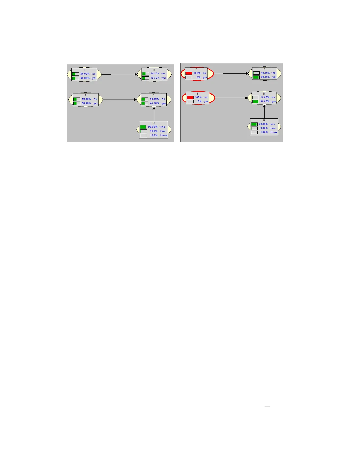
On the Relationship b et w een Ba y esian Net w orks and Probabilistic Structural Causal Mo dels P eter J.F. Lucas 1 , Eleanora Zullo 2 & F abio Stella 2 1 F acult y of EEMCS, Univ ersity of Tw ente, Ensc hede, the Netherlands ICIS, Radb oud Universit y , Nijmegen, the Netherlands 2 Dipartimen to di Informatica, Sistemistica e com unicazion Univ ersity of Milano-Bicocca, Milan, Italy Email: p eter.lucas@ut w ente.nl, { fabio.stella,e.zullo2 } @unimib.it Marc h 31, 2026 Abstract In this paper, the relationship betw een probabilistic graphical mo dels, in particular Ba y esian net w orks, and causal diagrams, also called structural causal mo dels, is studied. Structural causal models are deterministic mo dels, based on structural equations or func- tions, that can b e provided with uncertaint y by adding indep enden t, unobserved random v ariables to the mo dels, equipp ed with probabilit y distributions. One question that arises is whether a Ba yesian net work that has obtained from exp ert kno wledge or learn t from data can b e mapp ed to a probabilistic structural causal model, and whether or not this has consequences for the netw ork structure and probability distribution. W e sho w that linear algebra and linear programming offer k ey metho ds for the transformation, and ex- amine prop erties for the existence and uniqueness of solutions based on dimensions of the probabilistic structural mo del. Finally , we examine in what wa y the semantics of the mo dels is affected by this transformation. Keyw ords: Causality , probabilistic structural causal mo dels, Ba yesian netw orks, linear algebra, experimental softw are. 1 In tro duction With the increasing in terest in c ausality b y the probabilistic reasoning communit y , sev eral researc hers, and in particularly Judea P earl [8], made a switc h from a graphical represen tation of uncertain interactions based on probability theory , tow ards a deterministic represen tation of causal in teractions with some added external uncertain influence. F or considerable time, Ba yesian net w orks (BNs) and related graphical mo dels, suc h as maximal ancestral graphs [9], w ere the main vehicle for researc h in probabilistic graphical mo dels [7]. Since t wo decades their role w as slowly tak en ov er b y structural causal netw orks (SCMs) [8]. This is a surprising shift, as originally all the effort was aimed at developing a causal represen tation of uncertaint y , for example by c ausal Bay esian net w orks [3], where the adjective ‘causal’ emphasises the aim of mo delling uncertain causality . The implications of this step, although nev er emphasised in a prominent wa y , are profound, as with a deterministic graphical representation many of the indep endence assumptions developed for probabilistic graphical mo dels no longer hold [6, 7]. 1 There are also other reasons to raise eyebro ws, b ecause if a local probability distribution is in terpreted as an uncertain causal mec hanisms, p ossibly pro vided with abstraction, why is it that causal mechanisms can b e b est captured by a deterministic relationship with some added uncertain ty? Recen tly , structural causal models are also attracting muc h atten tion from the deep learn- ing comm unity , as many mechanisms in nature and so cial science can b e b est understo o d in terms of causal diagrams (e.g [5]), and, in addition, suc h mec hanisms, once mo delled as causal diagrams, can b e used to reliably generate syn thetic data, as demonstrated by Hollmann et al. [4]. Th us, structural causal mo dels can act as output of a mac hine learning pro cess, but they offer also p otential as input to the learning process. How ever, also in these situations, uncertain ty will p op up. These developmen ts clearly sho w that understanding the nature of causal diagrams is not only of in terest to a small group of researchers. Th us, an attempt to understand the relationship b et ween graphical mo dels used for un- certain ty representation and those for the representation of causal kno wledge appears to b e a go o d starting p oint for research. Part of the reasons for moving to causal netw orks deriv es from the fact that probabilistic relationships can b e reversed, using Ba yes’ rule, whic h is a phenomenon that do es not fit w ell with the principle of causalit y . Ho wev er, there are also certain practical reason wh y this switc h to deterministic equations is made. It is this whic h w e w ant to explore in this pap er, with as as sub question whether this switc h is alwa ys required and p ossible. One p oint which we wan t to raise is that probabilit y distributions can also b e deterministic, thus also violating some of the basic indep endence axioms of p ositiv e distri- butions, implying that in man y cases it is possible to use probabilistic graphical mo dels, or Ba yesian net w orks in our case, to implement causalit y . The most imp ortan t issue w e wish to shed light on is the relationship b et ween structural causal net work mo dels, and in particular their probabilistic extension, pr ob abilistic structur al c ausal mo dels (PSCMs), and Bay esian net works. Are they equiv alent, and is it alwa ys p ossible to transform one into the other and vice v ersa? The pap er is organised as follows. W e start with a brief motiv ating example to illustrate the problem that is being studied in the presen t paper. The example is follo wed by a summary of the mathematical concepts needed to b e able to answ er the researc h questions with some precision. The rest of Section 3 consists of a discussion of sev eral simple examples; it is hard to gain a feeling on the sub ject of causality if one resorts to presenting only abstractions. Next, we delve into issues concerning probability distributions of the exogenous v ariables, essen tially the probabilistic extension of deterministic causal models, in Section 4. The real no vel contributions of the pap er to the theory of probabilistic structured causal mo dels starts in Section 5, where w e sho w that w ell-known methods from linear algebra, and in particular linear programming, are k ey to unrav elling the relationships b et ween BNs and PSCMs. A p ython program that implements the theory dev elop ed in the pap er, supp orting exp erimen- tation with the transformation of BNs to PSCMs, is presen ted in Section 6. The pap er is concluded b y a brief discussion in Section 7. 2 Motiv ating example Before going into details of the mathematical machinery that is needed, we start b y providing a very simple instance of the kind of problems studied in this pap er, concerning tr e atment T and its effect B , here standing for blindness . 2 (a) (b) Figure 1: Tw o different Ba yesian net work represen tations of the same distribution; the top one a regular Bay esian net work, whereas the one at the b ottom is a Ba yesian netw ork repre- sen tation of a probabilistic structured causal mo del; (a): priors; (b) p osteriors. In the Ba yesian netw ork (BN) shown in Figure 1, the (uncertain) relationship betw een T and B is represented as the joint probability distribution P ( T , B ) = P ( B | T ) P ( T ), with conditional distributions: P ( B = n | T = n ) = 0 . 01 (1) P ( B = n | T = y ) = 0 . 99 (2) The following meaning is assumed: T = y (resp. T = n ) stands for treatmen t (no treatment) and B = y (resp. B = n ) stands for b eing blind (not b eing blind). Although T is intended as an interv ention, it will be represen ted as a random v ariable T that is uniformly distributed. The top of Figure 1 ((a) and (b)) depicts the asso ciated prior and instan tiated Ba yesian net work with p osteriors. The aim is to represen t this distribution by a probabilistic structured causal mo del (PSCM), with a causal relationship b et ween T and B , no w called ‘endogenous’ v ariables. Uncertain ty comes from outside, by a so-called ‘exogenous’ v ariable R . All v ariables are bi- nary . The relationship b etw een treatment T and the presence or absence of blindness B can b e represen ted by the function f B ( T ) = 1 − T = B The intuitiv e meaning is that treatment ( T = 1) prev ents a p erson from b ecoming blind ( B = 0). As we wish to represent this PSCM as a BN, adding uncertaint y to this deterministic relationship and function can b e done by adding an extra exogenous v ariable R to B , as is sho wn in Figure 1 ((a) and (b)) at the b ottom, and adding R to the conditional probabilit y distributions as follows: P ( B = n | T = y , R = n ) = 0 P ( B = n | T = y , R = y ) = 1 P ( B = n | T = n, R = n ) = 1 P ( B = n | T = n, R = y ) = 0 3 If we assume that the uncertaint y in R is represented b y the following distribution P ( R = y ) = 0 . 99 and P ( R = n ) = 0 . 01. This will allow to use only one unconditional binary distribution P ( R ) to represent the uncertaint y of two conditional distributions in this sp ecial case, as it is p ossible to compute P ( B | T ) as follo ws using the marginalisation rule: P ( B | T ) = X r P ( B , R = r | T ) = X r P ( B | T , R = r ) P ( R = r ) (3) As Figure 1 indicates, w e will get exactly the same conditional distributions P ( B | T ) for b oth cases, BN and BN version of the PSCM, top and b ottom. The reason why the binary distribution P ( R ) suffices for representing two conditional distributions P ( B | T = n ) and P ( B | T = y ) is due to the sp ecial case that P ( B = x | T = n ) = 1 − P ( B = x | T = y ) in all cases for x ∈ { n, y } : not more than t wo probabilities can b e exploited and in this case, not more than tw o are needed. Clearly , this will not hold for the general case, but it is unclear how many probabilities are needed in general. Also unclear is ho w the structural causal functions should b e defined based on a giv en Bay esian netw ork. Ho wev er, in order to precisely analyse the problem, some mathematical foundations hav e to b e pro vided, which will b e done in the following section. 3 Mathematical preliminaries W e start b y providing a short mathematical summary of the formal concepts that will b e utilised in the remainder of this pap er. 3.1 Ba yesian netw orks Let G = ( V , A ) b e an acyclic dir e cte d gr aph (DA G), with no des V = { 1 , 2 , . . . , n } , n ≥ 0, and ar cs A ⊆ V × V . The set of p ar ents of no de v ∈ V , denoted pa( v ), is defined as pa( v ) = { u | ( u, v ) ∈ A } . Definition 1 (Bay esian net work (BN)) . A Bayesian network B = ( G, X , P ) is defined as an acyclic directed graph G = ( V , A ), where the nodes hav e a 1–1 corresp ondence with the r andom variables X whic h are indexed by elements in V , i.e. X V = { X v | v ∈ V } . The asso ciated (discrete) joint pr ob ability distribution P of B is factorised as follows: P ( X V ) = Y v ∈ V P ( X v | X pa( v ) ) (4) V alues of a set of v ariables X are often denoted by X = x , or sometimes simply b y x . An arc ( v, w ) ∈ A is also denoted b y v → w . The asso ciated domain of X S , S ⊆ V , is denoted b y D ( X S ). In examples often no distinction is made b etw een no de v and v ariable X v , in particular when the no des get a descriptive name. Thus, a Bay esian net work is fully sp ecified b y its set of asso ciated conditional probability distributions P ( X v | X pa( v ) ), one distribution for each set of v alues x pa( v ) of the v ariables X pa( v ) , that take in to account the indep endence information encoded in the graph G . 3.2 Structural causal mo dels Structural causal mo dels are also defined as an acyclic directed graph as ab o v e for Ba yesian net works. 4 Definition 2 (Structural causal mo del (SCM)) . A structur al c ausal mo del M = ( G, X , F V ) is defined as an acyclic directed graph G = ( V , A ) with a 1–1 corresp ondence b et ween nodes V and v ariables X V , where the set of functions F V describ es c ausal r elations and is defined as follo ws: F V = { f v : D ( X pa( v ) ) → D ( X v ) | v ∈ V } (5) The functions f v are often represented as equations, not necessarily linear. So far, there is no uncertain ty inv olv ed in SCMs, as the functions f v are deterministic, and could also b e represented as a Ba yesian net work B where the functions f v are represen ted as a family of deterministic conditional probability distributions P ( X v | X pa( v ) ), i.e. with P ( x v | x pa( v ) ) ∈ { 0 , 1 } . Ho wev er, it is p ossible, as already demonstrated in Section 2, to extend a causal net work b y adding additional, uncertain so-called exo genous v ariables U W (and exogenous no des W = { n + 1 , . . . , m } ) to an SCM, where X V are now called endo genous v ariables, yielding a pr ob abilistic structur al c ausal mo del (PSCM) M = ( G, X , U, P ′ ) [11], with G = ( V ∪ W , A ), A ⊆ (( V ∪ W ) × V , with only one arc ( w , v ) ∈ A , for each w ∈ W and v ∈ V , and asso ciated join t probability distribution P ′ ( X V , U W ) = Y v ∈ V P ′ ( X v | X pa( v ) ) Y w ∈ W P ′ ( U w ) . (6) Note that the v ariables U w , w ∈ W , are assumed to b e independent, i.e. P ′ ( U W ) = Y w ∈ W P ′ ( U w ) and that paren ts pa( v ) include endogenous and exogenous no des. In addition, the conditional probabilit y distributions P ′ ( X v | X pa( v ) ) are deterministic and follow the sp ecification of the asso ciated functions f v of the SCM. Th us, the only uncertaint y represented in a PSCM is in its asso ciated exogenous v ariables U w . W e follow Zaffalon et al. [11] in emplo ying a sp ecial notation for parents of endogenous v ariables with the exogenous v ariable remov ed: X pa( v ) = X pa( v ) \ U W , for each v ∈ V . Note that, given the joint probability distribution P ′ ( X V , U W ), one can compute the probabilit y distribution P ′ ( X V ) simply by maginalisation: P ′ ( X V ) = X u W ∈ D ( U W ) P ′ ( X V , U W = u W ) and the resulting P ′ ( X V ) will in general b e nondeterministic. As w e also hav e that P ′ ( X V ) = Y v ∈ V P ′ ( X v | X pa( v ) ) where P ′ ( X v | X pa( v ) ) will not be deterministic in most cases, the question is whether it is p ossible to reco ver the conditional probabilit y distributions P ( X v | X pa( v ) ) based on the giv en P ′ ( U W ) and (deterministic) P ′ ( X v | X pa( v ) ), suc h that P ( X v ) = P ′ ( X v ). The solution provided b y Zaffalon et al. [11] makes use of the relationship b et ween a giv en endogenous v ariable X v and asso ciated exogenous v ariable U w , with ( w , v ) ∈ A ; the function f v maps u w and x pa( v ) to x v , as follows: f v : D ( U w ) × D ( X pa( v ) ) → D ( X v ) 5 i.e. f v ( u w , x pa( v ) ) = f v ( x pa( v ) ) = x v ∈ D ( X v ). As each tuple of v alues ( u w , x pa( v ) ) is mapp ed to a v alue x v of X v , each v alues of D ( X v ) co vered, the function f v is assumed to be surjective, and not necessarily injective. It ma y be that more than one tuple ( u w , x pa( v ) ) is mapped to the same x v , but each element of D ( X v ) has at least one asso ciated tuple from D ( U w ) × D ( X pa( v ) ). The surjectivity of f v implies that there exist a right in v erse function f − 1 v , when restricted to a fixed pa( v ), an in verse partial function is obtained: f − 1 v | pa( v ) : D ( X v ) → ℘ ( D ( U w )) i.e. f − 1 v | pa( v ) ( x v ) may yield a set of v alues from D ( U w ), whic h is a consequence of the surjectivity of f v . If f v is also injectiv e, then the range of f − 1 v | pa( v ) will consist of singleton sets, which also ma y b e represen ted b y their elemen ts. The requirement of surjectivit y of f v | pa( v ) comes from the requirement that ev ery element of D ( U w ) needs to map to at least one elemen t of D ( X v ). This will allow computing the elements of P ′ ( x v | x pa( v ) ) as follows: P ′ ( x v | x pa( v ) ) = X u w ∈ f − 1 v | pa( v ) ( x v ) P ′ ( U w = u w ) (7) A consequence of this definition is that P ′ ( x v | x pa( v ) ) can b e approximated b y a uniform distribution P ′ ( U w ), similarly to a Riemann sum (take as many v alue of U w , and sum the asso ciated probabilities, as needed to obtain P ′ ( x v | x pa( v ) )), for appropriate definitions of f v . Ho wev er, this approach w ould mak e P ′ ( U w ), and th us also P ′ ( x v | x pa( v ) ), meaningless. This implies that the meaning of P ′ ( U w ) would b ecome unimportant, which clearly is unacceptable, as what would b e the v alue of a meaningless causal net w ork? Emplo ying the righ t in verse of the function f v is not the only wa y to compute P ′ ( X v | x pa( v ) ), as giv en P ′ ( U w ) , w ∈ W , we can also determine P ′ ( X v | x pa( v ) ) for an y v alue of x pa( v ) ∈ D ( X pa( v ) ) using marginalisation as follows: P ′ ( X v | x pa ( v ) ) = X u w ∈ D ( U w ) P ′ ( X v | x pa( v ) , U w = u w ) P ′ ( U w = u ) (8) whic h offers a differen t approach, with essentially the same relationship betw een P ′ ( U w ) and P ′ ( X v | x pa( v ) ). Using either of the tw o approaches, the issue is whether or not the BN B can b e transformed to a PSCM M , and bac k, yielding the same BN, and vice versa, or P ( X v | X pa( v ) ) = P ′ ( X v | X pa( v ) ) for eac h v ∈ V , and th us whether P ( X V ) = P ′ ( X V ). Example 1. The conditional probabilities of the top BN of Figure 2 are defined as follows: P ( B = n | T = n ) = 0 . 1 P ( B = n | T = y ) = 0 . 99 Th us, in contrast to the motiv ating example of Section 2, these t wo probabilities no longer add up to 1, implying that the t wo probabilit y distributions can no longer b e represen ted by 6 (a) (b) Figure 2: Two different Ba yesian netw ork representations with tw o conditional distributions and more v alues for R , b efore and after en tering an in terv en tion T ; (a): priors; (b): posteriors. a single unconditional binary distribution, P ( R ) in this case. With a probability distribution of R consisting of three different v alues: P ( R = one) = 0 . 9 P ( R = tw o) = 0 . 09 P ( R = three) = 0 . 01 where inten tionally 0 . 9 + 0 . 09 = 0 . 99 and 0 . 09 + 0 . 01 = 0 . 1, and the asso ciated family of deterministic probabilit y distributions: P ( B = n | T = y , R = one) = 1 P ( B = n | T = y , R = tw o) = 1 P ( B = n | T = y , R = three) = 0 P ( B = n | T = n, R = one) = 0 P ( B = n | T = n, R = tw o) = 1 P ( B = n | T = n, R = three) = 1 using equation (3) it is p ossible to select the first t wo probabilities of P ( R ) to obtain P ( B = n | T = y ) and the last tw o probabilities to obtain P ( B = n | T = n ), as shown on the righ t-hand side of Figure 2. As a consequence, the tw o BNs in Figure 2 are equiv alen t, and after marginalisation out R , identical. Corresp onding to the deterministic conditional distributions ab o v e, is the following defi- nition of f B : f B ( T , R ) = ( T = 0) · ( R < 2) + T · ( R > 2) = B e.g. f B (1 , 2) = 0 = B (not blind, i.e. B = n ). The computations by using the marginalisation rule (equation (3)) are very similar to the use of the inv erse partial function f − 1 v | pa( v ) with t w o v alues (0.9 and 0.09) from D ( R ) associated to B = n | T = y and tw o other v alues (0.09 and 0.01) associated to B = n | T = n . Note that the v alue 0.09 is used t wice in the computations, one time to obtain P ( B = n | T = y ) and another time to obtain P ( B = n | T = n ). The 7 in verse of the partial function f B | T =1 , denoted f B | T = y , i.e. f − 1 B | T = y , w ould give the result f − 1 B | T = y (0) = { 1 , 2 } = { one , t wo } . The alternative computation based on Equation (7) w ould yield X r ∈ f − 1 B | T = y (0) P ( R = r ) = 0 . 9 + 0 . 09 = 0 . 99 = P ( B = n | T = y ) Th us, by decomp osing the conditional probabilities P ( X v | X pa( v ) ) in a prop er w ay giving rise to P ( U w ), and the righ t definition of the deterministic conditional probabilities P ( x v | x pa( v ) ), it is p ossible to recov er a Ba yesian net work in this wa y . The reader has probably already noticed that the definition of P ( R ) in Example 1 is not the only p ossibilit y to recov er the Ba yesian netw ork, whic h will b e demonstrated next. Example 2. Reconsider Example 1 with the giv en family of conditional probabilit y distri- butions P ( B | T ). As we wish to reco v er the probabilities 0.99 and 0.1 from P ( R ), a simple other definition is obtained by realising that 0.99 is obtained by the sum 0 . 89 + 0 . 1 This implies that the following P ( R = one) = 0 . 89 P ( R = tw o) = 0 . 1 P ( R = three) = 0 . 01 ma y also b e a suitable definition to recov er the Bay esian net work from a PSCM. How ever, when accepting this definition, the deterministic probabilit y distributions also needs to b e mo dified, as follows: P ( B = n | T = y , R = one) = 1 P ( B = n | T = y , R = tw o) = 1 P ( B = n | T = y , R = three) = 0 P ( B = n | T = n, R = one) = 0 P ( B = n | T = n, R = tw o) = 1 P ( B = n | T = n, R = three) = 0 This leads for example to: P ( B = n | T = y ) = X r P ( B = n | T = y , R = r ) P ( R = r ) = 1 · 0 . 89 + 1 · 0 . 1 + 0 · 0 . 01 = 0 . 99 After redefining the functions f B | T , the same result would b e obtained using Equation (7). 4 Relationship b et w een exogenous and endogenous v ariables 4.1 Ho w many v alues do w e need? Based on the discussion ab o ve, an obvious question is how Equations (7) and (8) would work if all v ariables in a PSCM, including the exogenous v ariables U w , w ∈ W , were assumed to b e binary , or whether a Bernoulli P ( U w ) would be able to capture the uncertain ty in the original BN (whic h may or may not hav e b een learn t from data). This is illustrated by means of the follo wing example. 8 Example 3. Returning to the motiv ating example in Section 2 and Figure 1, application of Equation (8) is easy in this case, as the set ℘ ( D ( U w )) = ℘ ( D ( R )) only contains tw o singleton sets { y } , { n } with the asso ciated probabilities copied once from P ( B = n | T = y ) and once from P ( B = n | T = n ). Equation (7) will give the same result. F or b oth conditional probability distributions w e ha ve the sp ecial case that P ( B = x | T = n ) = 1 − P ( B = x | T = y ) for x ∈ { n, y } . This sp ecial condition is needed, as P ( R ) only giv es tw o probabilities, namely P ( R = y ) and P ( R = n ) with P ( R = y ) = 1 − P ( R = n ). As P ( R ) is used to render the conditional probabilities P ( B | T , R ) uncertain, not more than t wo probabilities can b e exploited, whereas four are needed in general when the tw o conditional probabilities do not add to 1. The example giv en ab ov e sho ws that the approac h provided b y Zaffalon et al. [11] requires kno wledge ab out the distributions of b oth endogenous and exogenous v ariables before one can start using Equations (7) and (8). Although Example 1 indicates that the method will not w ork for arbitrary conditional distributions and a binary distribution, the approac h supp orts defining non-binary distributions of the exogenous v ariable. One needs first to fix a domain D ( U w ) with sufficient n umber of v alues. By constituting subsets of v alues of D ( U w ), prob- abilities can be combined in suc h wa y , by summing ov er the probabilities asso ciated with a subset v alues, that the conditional probabilities P ( x v | x pa( v ) ) can b e recov ered. This pro cess is discussed in the following section. 4.2 F orm ulation of the general case Definition 3 (Partition of domain) . Let X be a v ariable, with domain D ( X ) and discrete probabilit y distribution P ( X ), then Π( X ) denotes a p artition of domain D ( X ) consisting of subsets S ⊆ D ( X ), suc h that S S ∈ Π( X ) S = D ( X ) — a partition is exhaustiv e —, and each S, S ′ ∈ Π( X ), S  = S ′ , are disjoint. This concept of partition of a domain is needed for extracting probabilistic information from the exogenous v ariables, and will b e used to obtain matching probabilistic information for the endogenous v ariables. Definition 4 (Probability assignment) . Let U be an exogenous v ariable, P ( U ) its asso ciated discrete probabilit y distribution, and Π( U ) = { S 1 , . . . , S m } a partition of D ( U ). Let P ( x v | x pa( v ) ) b e the conditional probabilit y with U ∈ X pa( v ) and P ( x v | X pa( v ) ) = { P ( x v | x i pa( v ) ) | i = 1 , . . . , m } . A pr ob ability assignment is then defined as follo ws: P ( x v | x i pa ( v ) ) = X u ∈ S i P ( U = u ) . In Section 2 w e hav e discussed an example, where the partition of D ( R ) consisted of tw o singleton sets. Ho w ev er, any partition can b e used, not just singleton sets. In any case, the follo wing (obvious) prop osition holds: Prop osition 1. L et P ( x v | X p a ( v ) ) b e the r esult of a pr ob ability assignment, then it holds that: m X i =1 P ( x v | x i p a ( v ) ) = 1 9 Pr o of. As P u ∈ D ( U ) P ( U = u ) = 1, it follows that P S ∈ Π( U ) P u ∈ S P ( U = u ) = 1. The definition of a probabilit y assignment also supp orts using different permutations of probabilities, whic h essentially yield different probability distributions P ( U ), but b y putting the same combinations of probabilities into a partition, the same family of conditional prob- abilit y distributions can b e obtained. Ho wev er, as w as demonstrated by Examples 1 and 2, it is also p ossible to form clusters of probabilities from P ( U ) to define conditional probabilities, violating the requiremen t of a partition that its members are disjoin t and exhaustive. Example 4. The probability distributions P ( R ) defined in Examples 1 and 2 yield sets of clusters {{ 0 . 9 , 0 . 09 } , { 0 . 09 , 0 . 01 }} and {{ 0 . 89 , 0 . 1 } , { 0 . 1 }} , resp., which do not constitute a partition (since the first and second example ha v e o verlapping sets, where in addition for the second example the sets are not exhaustive) and in both cases Prop osition 1 do es not apply b ecause the partition requirement fails to hold. So far it is assumed that there is no knowledge represen ted in a giv en BN to build the causal relationships (5): F V = { f v : D ( X pa( v ) ) → D ( X v ) | v ∈ V } of a PSCM based on a given BN. In reality , how ev er, some relationships betw een paren t v ariables and a c hild v ariable are so strong (reflected by a high probability) that one ma y exp ect that they carry ov er to the causal functional relationship. Unfortunately , the exogenous v ariables thro w a spanner in the w orks. As its asso ciated probability distribution models the uncertain ty in the causal relationship, as we ha ve seen ab o ve, usually sev eral probabilities from this distribution are needed to (re)build the conditional probability distributions of a BN. By reordering a distribution of an exogenous v ariable (for example from high to lo w probabilit y), one can confidently sa y that the strong relationships must come from the high end of the distribution. How ever, not m uc h more can b e concluded from this observ ation. 4.3 Offers adding arcs an alternativ e metho d? As has b een demonstrated in the previous section, the probabilit y distribution of the exoge- nous v ariables P ( U W ) can b e used to add uncertaint y to the functional relationship b etw een causes and the effects expressed by the functions f v , but without having a clear meaning. It w as also shown that different probability distributions P ( U W ) can b e used to transform a BN to a PSCM and vise versa. Thus, as a preliminary conclusion it can b e stated that a relationship betw een BNs and PSCMs exists, although not necessarily unique. This conclusion raises the question whether there are alternativ e w ays to transform a BN in to a PSCM. Example 5. Reconsider the BN from Example 1. One p otential alternative solution is to add an arc from vertex T to R . This is done in Figure 3. T o b e able to represen t the same distribution using a deterministic causal net work, i.e. a PSCM, w e draw an arc from T to R and define P ( R | T ) as follo ws: P ( R = n | T = n ) = 0 . 1 (9) P ( R = n | T = y ) = 0 . 01 (10) 10 (a) (b) Figure 3: Two differen t Ba yesian netw ork represen tations of the same distribution with one extra arc from T to R with (a): priors; (b) posteriors. Using P ( B | T ) = X r P ( B , R = r | T ) = X r P ( B | T , R = r ) P ( R = r | T ) (11) w e are able to compute the distribution after conditioning on v alues for T , resulting in the same a p osterior distribution, as sho wn in Figure 3. The conditional probability distributions P ( B | T , R ) are the same as for Example 1: P ( B = n | T = y , R = n ) = 0 P ( B = n | T = y , R = y ) = 1 P ( B = n | T = n, R = n ) = 1 P ( B = n | T = n, R = y ) = 0 This shows that b y adding random v ariables to a Ba yesian netw ork after mo difying a set of uncertain conditional distributions to deterministic conditional distributions, it is p ossible to represen t the same conditional distribution, P ( B | T ) in our example, by adding an exogenous v ariable and adding an arc from the conditioning v ariable to the new, exogenous v ariable. Hence, an alternative metho d exists, but it is still very similar to the original metho d in tro duced earlier, and actually adds extra complexity to the metho d without offering a clear adv an tage. Because of this, the method will not b e pursued an y further. 5 T ransforming a BN to a PSCM The preceding section was primary mean t to provide a basic understanding of the p oten tial relationships b etw een BNs and PSCMs. In the present section we dev elop a deep er analysis of the relationship, and in particular we form ulate an answ er to the following questions: (1) is there a pro cedure for turning a Ba yesian netw ork into a PSCM, and (2) would that yield a causal netw ork that in some sense is equiv alent to the original BN? The w ay these questions are approac hed is b y turning to linear algebra, and in particular linear programming. It will b ecome clear in the following why this is a suitable approach. Assuming that we ha ve a family of conditional deterministic probabilit y distributions P ′ ( X v | x pa( v ) , U w = u w ), and a family of probabilit y distributions P ′ ( x v | x pa( v ) ), we will 11 solv e for P ′ ( U w = u w ). This pro cess is elaborated in the subsequent subsections, where first some common linear algebra concepts are reiterated. 5.1 Linear algebra notation and concepts W ork on algebraic formulation of probabilit y theory started with George Bo ole [1], whic h was later pick ed up again by Castillo et al. [2]. In the present con text, linear algebra offers a go o d starting point for analysis. Only a minimal amount of linear-algebra notation and concepts will b e rep eated here, based on the b o ok b y Strang [10], to a v oid misunderstanding in the notation used in the follo wing and to refresh the memory of some readers. A ve ctor sp ac e V consists of v ectors that are closed under addition and scalar m ultiplica- tion; the zero vector is alwa ys part of a v ector space. If a vector space V consists of all linear com binations of v ectors v 1 , v 2 , . . . , v n , i.e., v ∈ V if v = P n i =1 c i v i , with c i  = 0, i = 1 , . . . , n , n ≥ 0, then it is said that these vectors sp an the vector space, denoted L ( v 1 , . . . , v n ). A b asis for a vector space V is a set of vectors { v 1 , . . . , v n } that is line arly indep endent , i.e. P n i =1 c i v i  = 0 unless c 1 = c 2 = · · · = c n = 0, and that span the space. W e use upp er-case letters, such as A , for m × n matric es , with m × n its dimension , lo wer-cases letters for c olumn ve ctors , suc h as x , whereas r ow ve ctors are denoted b y the tr ansp ose of the column-v ector: x T . In addition, use will b e made of the c olumn sp ac e of a matrix A , denoted R ( A ), R stands for r ange , where A is interpreted as a linear transformation T A : R n → R m . A transformation T A ( x ) = b , with T A a linear transformation based on A , th us corresp onds to a set of linear equations Ax = b , with x ∈ R n and b ∈ R m . The maximal n umber of elemen ts of the subset of columns of a matrix A that span R ( A ) is called the r ank of A . It happ ens that the rank of the column space of A is equal to the rank of the ro w space of A , i.e., dim R ( A ) = dim R ( A T ) = r ( A ), despite the fact that the column space R ( A ) and ro w space R ( A T ) are usually differen t. The existence of a solution x of the equation Ax = b means that b is in the column space R ( A ) spanned by the column vectors of A . 5.2 Linear algebra form ulation Equation (8) is a linear equation, with P ′ ( X v | x pa( v ) , U w = u w ) ∈ { 0 , 1 } , whereas P ′ ( U w = u w ), for brevity represented as u w , can b e taken as a v ector: u =      P ′ ( U w = u 1 ) P ′ ( U w = u 2 ) . . . P ′ ( U w = u n )      =      u 1 u 2 . . . u n      The Boolean P ′ ( X v | X pa( v ) = x i , U w = u w ) can b e represented as an elemen t of a matrix A , with a ij = P ′ ( X v = x v | X pa( v ) = x i , U w = u j ) 12 Com bined, we get the follo wing inhomogeneous linear equation: Au =        a 1 , 1 a 1 , 2 · · · a 1 ,n a 2 , 1 a 2 , 2 · · · a 2 ,n . . . . . . . . . . . . a m − 1 , 1 a m − 1 , 2 · · · a m − 1 ,n 1 1 · · · 1             u 1 u 2 . . . u n      = b =        b 1 b 2 . . . b m − 1 b m        =         P ′ ( x v | x pa( v ) = x 1 ) P ′ ( x v | x pa( v ) = x 2 ) . . . P ′ ( x v | x pa( v ) = x m − 1 ) 1         The last row of A , together with b m , which consists of 1s only , follo ws from the fact that u is a probabilit y vector: P n i =1 u i = 1. F rom now on, it is assumed that vector b con tains a last, m th elemen t equal to 1. In solving the linear equation Au = b , with m × n matrix A , and both A and b known, there is at le ast one solution u if and only if the num b er of ro ws m is equal to the rank of the matrix A , r ( A ), i.e. m = r ( A ) [10]. Subsequently , it is assumed that P ( X v | x pa( v ) ) = P ′ ( X v | x pa( v ) ) for eac h x pa( v ) and v ∈ V , as this will giv e the required relationship b etw een PSCMs and BNs. No w, in contrast to what is common in solving linear equations, in the present case b oth A and u are unknown , and only b is known. That clearly indicates that it may not b e easy to come up with a solution. What helps, how ev e r, is that we know that the matrix A is Bo olean (or binary), a ij ∈ { 0 , 1 } , and that we need at least r ( A ) linear indep enden t column vectors a from A that span the column space of A . As A is unknown, we could generate those linear indep enden t column vectors based on a fixed dimension and p otentially based on the original conditional probabilities P ( x v | x pa( v ) ), and solve for u . This generation pro cess is clearly the most straigh tforward wa y to tac kle this problem. 5.3 T ow ards linear programming The form ulation ab ov e is incomplete, as a solution u ma y include negativ e elements and elemen ts bigger than 1, ev en though the sum of the comp onents of u is guaranteed to sum to 1. W e can solv e this either by linear programming (LP for short), where most of the constrain ts are equality constraints, or by solving the set of linear equations b y standard linear algebra, and if a solution is found, chec king whether it satisfies the constrain ts of a probabilit y distribution. The only adv an tage of linear programming in this case is that its feasible solutions are guaran teed to satisfy the inequality constraints as well. As the simplest solution is that of solving a set of linear equations, we discuss that particular approac h first. In order to handle the inequalities with resp ect to u mentioned ab ov e, it is necessary to include extra constraints to the linear equation Au = b . W e need to add the constraints that 0 ≤ u i ≤ 1, for eac h i = 1 , . . . , n . This is done b y adding a kind of slack variables w i to the probabilit y vector u expressing the situation that u i ≤ 1, for i = 1 , . . . , n , i.e. w i = 1 − u i ⇔ u i + w i = 1 with u i , w i ≥ 0, for i = 1 , . . . , n . The extended linear equation A ′ x = b ′ that is obtained, no w has one extra constraint that x = [ u w ] T ≥ 0: A ′ u ′ =  A O I I   u w  =  b e  = b ′ 13 with I the n × n iden tity matrix, e = [1 1 · · · 1] T the column vector with 1s, and O the m × n n ull matrix (with zeros). Recall that the last row of A and also of O enforce that u is a probabilit y vector. Next we demonstrate how to use this approac h to transform a simple Ba yesian net work, b efore mo ving on to other issues such as the n umber of elements of probability vector needed to be able to p erform the transformation. Example 6. Reconsider Example 1 and Figure 2. F ormulated as a linear equation with constrain ts, the probabilities presen ted in the example can b e represen ted as follows: A ′  u w  =  A O I I   u w  =         1 1 0 0 0 0 0 1 1 0 0 0 1 1 1 0 0 0 1 0 0 1 0 0 0 1 0 0 1 0 0 0 1 0 0 1          u w  = b ′ =         0 . 99 0 . 1 1 1 1 1         with solution v ector x = [ u w ] T ≥ 0. A unique solution is [ u w ] T = [0 . 9 0 . 09 0 . 01 0 . 1 0 . 91 0 . 99] T , where u are v ariables and w the constraint (slack) v ariables. In this case, w e ha ve that the rank of A ′ , r ( A ′ ) = 6. As A ′ is a 6 × 6 square matrix, the matrix is in vertible if it is non- singular (the righ t inv erse is equal to the left in v erse), and that a solution [ u w ] T exists for an y v ector b ′ . Observ e that the vectors u and w satisfy the sp ecified constraint that u i + w i = 1, i ≤ i ≤ 3. In this case, the corresp onding probabilit y distribution of R consisting of three differen t v alues is: P ( R = one) = 0 . 9 P ( R = tw o) = 0 . 09 P ( R = three) = 0 . 01 This unique solution is also a feasible solution obtained by linear programming. Next, consider the matrix A ′′ : A ′′ =         0 1 0 0 0 0 0 1 1 0 0 0 1 1 1 0 0 0 1 0 0 1 0 0 0 1 0 0 1 0 0 0 1 0 0 1         The only difference with A ′ is in comp onen t a 11 . In this case, solving the corresp onding set of linear equations yields: [ u w ] T = [0 . 9 0 . 99 − 0 . 89 0 . 1 0 . 01 1 . 89] T , where the probabilit y constrain ts are b eing violated. Linear programming will simply notice that a feasible solution do es not exist. The example ab ov e illustrates that the matrix A (the submatrix of A ′ ) does nothing else than selecting elements from the vector u suc h that the sum of those elements equals an elemen t b ′ i (with i = 1 , 2 in the example). The linear programming approac h offers something extra in comparison to the linear alge- bra approac h: its solution x optimises (minimises) a linear function c T x , called the obje ctive 14 function . This function can b e used to form ulate extra constrain ts on the solution vector x . Ho wev er, it is not immediately clear in what w ay to use the ob jectiv e function as part of retrieving the probability distribution of the original Ba yesian netw ork. 5.4 Existence and uniqueness of solutions of the sy stem of linear inequalities T aking the linear programming formulation as a start, i.e. A ′  u w  =  A O I I   u w  = b ′ with [ u w ] T ≥ 0, w e simplify the mathematical formulation for ease of exposition, by rewriting the abov e equation to A ′ x = b ′ with x = [ u w ] T ≥ 0, and min x c T x , the ob jectiv e function that is b eing minimised. Th us, from no w on, A ′ is tak en as an m × n matrix, x as an n -dimensional column vector, and b ′ as an m -dimensional column v ector. Whether A ′ is square ( m = n ), or rectangular with either m > n or m < n , is fully determined b y how many components of x (or actually sub v ector u ) are summed together to obtain comp onents of b ′ . The general rule is that the larger n is, the easier it b ecomes to reconstruct the original causal Ba yesian netw ork as there will b e more freedom in selecting probabilities. In other words, ho w man y probabilities P ( U w = u w ) are selected by the deterministic conditional probabilities P ′ ( X v = x v | x pa( v ) , U w = u w ), to obtain P ′ ( X v = x v | x pa( v ) ), i.e., b ′ , is gov erned by the matrix A ′ . The rank and the m × n dimension of the matrix A ′ allo w distinguishing v arious cases, where again we follow the b o ok by Strang [10]: • ( m = n ) The problem is to find a Bo olean submatrix A of A ′ , that, when em b edded in A ′ , is in vertible, yielding the elements of [ u w ] T from the multiplication A ′ − 1 b ′ . If A ′ is invertible , and thus a bijective linear transformation, then w e alw ays hav e a unique solution; x = A ′ − 1 b ′ , and the ob jectiv e function c T x used in linear programming simply yields a v alue that is also unique. The only use of linear programming here, in contrast to the standard linear algebra of equations, is to e nsure that u is a probabilit y v ector, and to disregard solutions that fail to meet that requiremen t. The rank of the matrix A ′ is equal to r ( A ′ ) = r = m = n , and w e hav e only basic v ariables and no free v ariables. Ho wev er, if r ( A ′ ) < n , then there are free v ariables. This situation is similar to what is discussed for the cases with m  = n below. • ( m > n ) The system A ′ x = b ′ has at most one solution if and only if the n columns of A ′ are linearly indep endent, i.e., r ( A ′ ) = r = n . In this case, A ′ is an injectiv e linear transformation, and there exists an n × m left-inverse matrix B , such that B A ′ = I n , with B = ( A ′ T A ′ ) − 1 A ′ T . How ever, if r ( A ′ ) = r < n , then there are r basic v ariables and n − r free v ariables. The free v ariables will allo w to generate an infinite n um b er of solutions. It is p ossible to select one p articular solution by assuming that all the free v ariables are zero. The ob jective function of linear programming is then based on the basic v ariables. How ever, we ma y also exc hange basic and free v ariables, as is common in linear programming, to mo ve to a different particular solution. If r ( A ′ ) = n , an LP solution will b e the same as the one obtained by the linear algebra approac h. 15 • ( m < n ) The system A ′ x = b ′ has at le ast one solution if the columns of A ′ span R m , i.e., r ( A ′ ) = r = m . There exists an n × m righ t-in verse C such that A ′ C = I m , with C = A ′ T ( A ′ A ′ T ) − 1 . If r ( A ′ ) < m , there are m − r constrain ts on b ′ for A ′ x = b ′ to b e solv able and there are r basic v ariables and n − r free v ariables. Ho wev er, as A ′ is a surjective linear transformation, the solution x obtained in this wa y is just one of the p ossible solutions (see Examples 2 for an actual case), and ma y differ from the LP solution. W e giv e a num b er of examples to illustrate the theory presen ted ab ov e. Example 7. W e adopt the same order of cases distinguished ab ov e. • ( m = n ). F or the m × n matrix A ′ it holds that r ( A ′ ) = m = n , i.e., the matrix is non-singular and an inv erse A ′ − 1 exists. Here m = n = 6 = r ( A ′ ), and b ′ = [0 . 99 0 . 1 1 1 1 1] T A ′ =         1 1 0 0 0 0 1 0 0 0 0 0 1 1 1 0 0 0 1 0 0 1 0 0 0 1 0 0 1 0 0 0 1 0 0 1         resulting in the LP solution: x = [0 . 1 0 . 89 0 . 01 0 . 9 0 . 11 0 . 99] T A ′ − 1 =         0 1 0 − 0 0 − 0 1 − 1 0 − 0 0 − 0 − 1 0 1 − 0 0 − 0 0 − 1 0 1 0 − 0 − 1 1 0 0 1 − 0 1 0 − 1 0 0 1         Clearly , A ′ − 1 b ′ = x = [0 . 1 0 . 89 0 . 01 0 . 9 0 . 11 0 . 99] T , which is exactly the same as the LP solution men tioned ab ov e. • ( m > n ). The m × n matrix A ′ has an n × m left inv erse B as m > n . In the example b elo w, m = 7, n = 4 = r ( A ′ ), and b ′ = [0 . 1 0 . 9 0 . 1 0 . 9 1 1 1] A ′ =           1 0 0 0 0 1 0 0 1 0 0 0 0 1 0 0 1 1 0 0 1 0 1 0 0 1 0 1           16 with LP solution equal to x = [0 . 1 0 . 9 0 . 9 0 . 1] T . The left inv erse B is equal to: B =     0 . 375 − 0 . 125 0 . 375 − 0 . 125 0 . 25 0 0 − 0 . 125 0 . 375 − 0 . 125 0 . 375 0 . 25 0 0 − 0 . 375 0 . 125 − 0 . 375 0 . 125 − 0 . 25 1 0 0 . 125 − 0 . 375 0 . 125 − 0 . 375 − 0 . 25 0 1     with B b ′ = x = [0 . 1 0 . 9 0 . 9 0 . 1] T . • ( m < n ). There is only an n × m righ t inv erse C and r ( A ′ ) = m . Here, m = 7 = r ( A ′ ) and n = 8, with b ′ = [0 . 99 0 . 1 1 1 1 1 1] T and A ′ =           0 1 1 1 0 0 0 0 0 0 0 1 0 0 0 0 1 1 1 1 0 0 0 0 1 0 0 0 1 0 0 0 0 1 0 0 0 1 0 0 0 0 1 0 0 0 1 0 0 0 0 1 0 0 0 1           with LP solution equal to x = [0 . 01 0 . 89 0 0 . 1 0 . 99 0 . 11 1 0 . 9] T . The right in verse C is equal to: C =             − 1 0 1 0 0 0 0 0 . 5 − 0 . 5 0 0 0 . 25 − 0 . 25 0 0 . 5 − 0 . 5 0 0 − 0 . 25 0 . 25 0 0 1 0 0 0 0 0 1 0 − 1 1 0 0 0 − 0 . 5 0 . 5 0 0 0 . 75 0 . 25 0 − 0 . 5 0 . 5 0 0 0 . 25 0 . 75 0 0 − 1 0 0 0 0 1             Here it holds that C b ′ = x ′ = [0 . 01 0 . 445 0 . 445 0 . 1 0 . 99 0 . 555 0 . 555 0 . 9] T . Note that the LP and the linear algebra solution differ. F or the LP solution x with c T = [10 1 1 1 1 1 1 1], we hav e that c T x = 3 . 09, whereas the linear algebra solution x ′ yields c T x ′ = 4 . 09, whic h explains wh y it was not selected by LP . 5.5 P ermutations of solutions In this section, we fo cus on the submatrices A of A ′ and vector u . Let A and A l b e tw o Bo olean matrices, where A l is obtained from A b y pre-multiplying A b y a p ermutation matrix P , basically the identit y matrix I with ro ws reordered, with A l = P A ; in other words, A l is the same as A with ro ws reordered. F or the solutions of the set of equations A l u = b w e hav e that A l u = P Au = b ⇔ Au = P − 1 b = P T b = b ′ 17 (as p ermutation matrices are orthogonal matrices, they hav e the sp ecial prop erty that P − 1 = P T ) which implies that that the solution u do es not c hange. Ho w ev er, the solution of Au ′ = b is likely to b e differen t from A l u = b as for the row space it holds that R ( A T ) = R ( A T l ), but b should b e in the column space R ( A ), and the column spaces R ( A ) and R ( A l ) are likely to differ. Th us, rather than considering reordering the ro ws, we should consider columns of A . W e ha ve that the column space R ( A ) remains the same despite column reordering, meaning that b ∈ R ( A ) if the equation Ax = b has a solution x , then also b ∈ R ( A r ), with A r = AP , i.e. A after p ost-multiplication b y the p ermutation matrix P . Hence, a starting p oint for reducing (p oten tially) irrelev ant p ermutations of solution vector u is by reducing the num b er of reorderings of columns of a previously generated Bo olean matrix A . The following example will demonstrate that a p ermutation of a matrix A will not alwa ys yield a p ermutation of a solution. Example 8. W e demonstrate the consequences of pre- and p ost-m ultiplication by a p ermu- tation matrix P . Let b = [0 . 99 0 . 1] T in the equation Au = b , with A =  1 1 0 0 1 0  a (probabilit y vector) solution is u = [0 . 89 0 . 1 0 . 01] T . No w, let A l =  0 1 0 1 1 0  = P A =  0 1 1 0   1 1 0 0 1 0  b e a reordering of A ; a solution is u ′ = [ − 0 . 89 0 . 99 0 . 9] T , whic h is neither a permutation of u nor a probability vector. Subsequently , consider A r = AP ′ = A   0 1 0 1 0 0 0 0 1   =  1 1 0 1 0 0  where w e reordered the columns of matrix A . The set of equations A r u ′′ =  1 1 0 1 0 0  u ′′ = b yield u ′′ = [0 . 1 0 . 89 0 . 01] T , which is a p ermutation of u , and a probability v ector. Another p erm utation is obtained by A ′ r = AP ′′ = A   0 0 1 0 1 0 1 0 0   =  0 1 1 0 1 0  where again we reordered the columns of matrix A . The set of equations A ′ r u ′′′ =  0 1 1 0 1 0  u ′′′ = b yield u ′′′ = [0 . 01 0 . 1 0 . 89] T , whic h is another p erm utation of u , and a probabilit y vector. 18 The example illustrates the following simple equiv alence. Prop osition 2. L et u b e a solution of the set of line ar e quations Au = b , then if AP u ′ = A r u ′ = b , with solution u ′ and p ermutation matrix P , t hen ve ctor u is a p ermutation of ve ctor u ′ and vic e versa. Pr o of. AP u ′ = A r u ′ = b ⇔ A ( P u ′ ) = b ⇔ Au = b , with u = P u ′ . This simple prop osition means that rather than first generating Bo olean matrices A , one can also generate, more efficien tly , p ermutations of solutions. Unfortunately , the prop osition do es not preven t redundancy in the generation process of matrices A . Ho wev er, whereas it is hard to come up with a w a y to prev en t generating redundan t matrices A , it is possible, at least partially , to bypass generating redundan t solutions. As discussed in Section 5.1, the existence of a solution u of Au = b is equiv alen t to the statement that b ∈ R ( A ), and the order of columns in A do es not matter. A simple approac h to preven t rep eatedly generating p erm utations of solution v ectors can b e obtained by chec king whether a particular column space R ( A ) has b een generated b efore. One can do this by first transforming a Boolean matrix A to a canonical form with preserv ation of the column space. Unfortunately , the actual transformation will cost (although polynomial) computation time. Alternatively , one can sort the columns of a matrix A for which a solution of the equation Au = b exists, and for an y newly generated matrix A ′ c heck whether the sorted v ersion of this matrix w as previously generated. If it do es, then clearly the solution u ′ of A ′ u ′ = b , which is guaran teed to exist, is a permutation of u . Prop osition 3. L et Au = b b e a system of line ar e quations with at le ast one solution ve ctor u , and let sort ( A ) = A ′ b e a matrix with the c olumns of A in lexic o gr aphic or der. Then, A ′ u ′ = b has a solution u ′ , with u ′ = P u , i.e. u ′ is a p ermutation of u and vic e versa, wher e P is a p ermutation matrix. Pr o of. Simply note that A ′ P u = Au = b . Clearly , Prop osition (3) is almost identical to Prop osition (2) except that Proposition (3) can be used to filter out matrices, once generated, from further pro cessing. 6 A heuristic searc h algorithm As suggested in the previous section: there is not alw ays a unique solution to the equation A ′ x = b ′ , with an unkno wn Bo olean submatrix A of A ′ , an unknown vector x = [ u w ] T , with u a probabilit y vector and slack v ariables w , and the known vector b ′ . The only thing we kno w b eforehand, namely that A is a Bo olean (binary) matrix, yields as a p ossible approac h to systematically generate the matrix A , and subsequen tly solv e for [ u w ] T using linear pro- gramming. This is what the p ython co de b elo w do es, where w e ha ve reco ded [ u w ] T simply as u (and u.x is the feasible linear programming solution). In addition, in the co de b elow, w e use the linear algebra approac h to the existence and uniqueness of solutions as an alternativ e to the LP approac h. This will allow exploring the alternativ e cases, based on the dimensions of the matrix A , in tro duced in Section 5.4. As a simple heuristic we use a cac he to store column sorted matrices A for whic h a solution was found using LP as a partially successful metho d to preven t generating the same p erm utated solutions multiple times. As men tioned ab ov e, a b etter method w ould chec k for 19 equiv alence of the column space of the matrix, but that w ould b e even more time consuming. Finally , it is, in principle, also p ossible that for tw o differen t matrices A, A ′ it holds that Au = A ′ u = b , i.e. the same solution u is obtained. W e give an example b elo w. Example 9. Consider the following tw o examples: A =         1 0 0 0 0 1 1 1 1 0 0 1 0 0 0 0 1 1 0 0 0 0 1 0 0 1 1 1 1 1         u = [0 . 1 0 . 4 0 . 3 0 . 19 0 . 01] T A ′ =         1 0 0 0 0 1 1 1 1 0 0 1 0 0 0 0 1 1 0 0 1 0 0 1 1 1 1 1 1 1         u ′ = [0 . 1 0 . 4 0 . 3 0 . 19 0 . 01] T The t wo matrices A, A ′ differ, and yet the solution obtained is iden tical The python co de presented b elow, that was dev elop ed according to the theory elab orated in the section ab ov e, supp orts exp erimen tation of the pro cess of transforming a BN to a PSCM. import numpy as np from scipy import linalg, optimize import copy def Ext(setofsets, add): """ add new elements to each set of powerset """ temp = copy.deepcopy(setofsets) l = len(setofsets) for i in range(l): setofsets[i].append(add) # setofsets is mutated temp.extend(setofsets) return temp def Powerset(set): """ compute powerset of set """ 20 if len(set) != 0: car = set.pop(-1) return Ext(Powerset(set), car) else: return [[]] def ComputeSolutions(m, n, b, limit): A = np.zeros((m+1, n)) indices = list(range(0, n)) ps = Powerset(indices) pslist = list(range(0, m)) for i in range(0, m): pslist[i] = copy.deepcopy(ps) pslist[i].pop(0) # remove empty list O = np.zeros((m+1, n)) # not used, just for consistency with theory I = np.eye(n) e = np.ones(n) A[m, 0:n] = e o = np.zeros(n) # not used, just for consistency with theory Ap = np.zeros((m + n + 1, 2 * n)) Ap[0:m+1, 0:n] = A Ap[m+1:(n + m + 1), 0:n] = I Ap[m+1:(n + m + 1), n:(2 * n)] = I Solve(Ap, A, m, n, pslist, [], limit) def Occurs(A, arraylist): """ Array A is member of a list of arrays """ if arraylist == []: return(False) elif np.all(A == arraylist.pop()): return(True) else: return(Occurs(A, arraylist)) def Solve(Ap, A, m, n, sos, cache, limit): """ vary in indices recursively going through set of sets (sos); limit is largest size of list that is used, to reduce the search under the assumption (heuristic) that smaller index sets are more likely to provide a solution. """ for set in sos[0]: if len(set) <= limit: A[m - len(sos), set] = 1 sortedarray = np.sort(A, 1) 21 if len(sos) > 1: Solve(Ap, A, m, n, sos[1:len(sos)], cache, limit) Ap[0:m + 1, 0:n] = A obj = np.ones(2 * n) if not(Occurs(sortedarray, cache.copy())): u = optimize.linprog(obj, A_eq = Ap, b_eq = b, bounds = (0, None)) if u.success: print("Successful matrix & solution:") print(Ap, "\n", u.x) if (Ap.shape[0] == Ap.shape[1]): det = linalg.det(Ap) if det == 0: print("\nSingular square matrix \n") else: Ainv = linalg.inv(Ap) u2 = np.dot(Ainv, b) print("\nInverse * b = ", u2, "\n") elif (Ap.shape[0] > Ap.shape[1]): leftinverse = np.dot(linalg.inv(np.dot(np.transpose(Ap),Ap)), np.transpose(Ap)) u2 = np.dot(leftinverse, b) print("\nLeftinverse * b = ", u2, "\n") else: rightinverse = np.dot(np.transpose(Ap), linalg.inv(np.dot(Ap,np.transpose(Ap)))) u2 = np.dot(rightinverse, b) print("\nRight inverse * b = ", u2, "\n") cache.append(sortedarray) A[m - len(sos), set] = 0 Next, an example run of the p ython co de with some solutions generated for Example 1 is sho wn: m = 2; n = 3; limit = 2 # Example 1 b = np.array([[0.99], [0.1], [1], [1], [1], [1]]) >>> ComputeSolutions(m, n, b, lim) Successful matrix & solution: [[1. 1. 0. 0. 0. 0.] [1. 0. 0. 0. 0. 0.] [1. 1. 1. 0. 0. 0.] [1. 0. 0. 1. 0. 0.] [0. 1. 0. 0. 1. 0.] [0. 0. 1. 0. 0. 1.]] 22 [0.1 0.89 0.01 0.9 0.11 0.99] Inverse * b = [[0.1] [0.89] [0.01] [0.9 ] [0.11] [0.99]] Successful matrix & solution: [[1. 1. 0. 0. 0. 0.] [1. 0. 1. 0. 0. 0.] [1. 1. 1. 0. 0. 0.] [1. 0. 0. 1. 0. 0.] [0. 1. 0. 0. 1. 0.] [0. 0. 1. 0. 0. 1.]] [0.09 0.9 0.01 0.91 0.1 0.99] Inverse * b = [[0.09] [0.9 ] [0.01] [0.91] [0.1 ] [0.99]] 7 Discussion In this pap er, we introduced a systematic w ay for transforming a BN to a PSCM. As there is already a significant amoun t of theory , including its implemen tations within soft w are envi- ronmen ts, to learn b oth graph structure and parameterisations of a BN from data, the idea of transforming a BN to a PSCM is app ealing. Practically sp eaking, one may start by develop- ing a BN from a mixture of data and exp ert knowledge, which, after having b een successfully ev aluated, may be turned into a PSCM. A requirement for a succe ssful transformation is that a PSCM’s exogenous v ariables are introduced with a domain consisting of sufficien t n umber of v alues to preserv e the probabilistic information. In addition, the causal functions or de- terministic conditional probability distributions that admit generating an equiv alence PSCM are usually not unique. Actually , the process of generating solutions has combinatorial prop- erties, and effectiv e heuristics to reduce the n um b er of alternative solutions generated ha ve not been found so far. One disadv an tage of a PSCM is its unclear seman tics as different definitions of probabilit y distributions of the exogenous v ariables ma y giv e equiv alen t results. This also raises doubts ab out the usefulness of PSCMs as a suitable alternativ e to BNs, certainly in the con text of mac hine learning. 23 References [1] George Bo ole. A n Investigation of the L aws of Thought: on Which ar e F ounde d the Mathematic al The ories of L o gic and Pr ob abilities . W alton and Mab erly , London, 1854. [2] Enrique Castillo, Jos ´ e Manual Guti ´ errez, and Ali S. Hadi. Exp ert Systems and Pr ob a- bilistic Network Mo dels . Springer-V erlag New Y ork, 1997. [3] Norman F enton and Martin Neil. Risk assessment and de cision analysis with Bayesian networks . CR C Press, 2012. [4] Noah Hollmann, Samuel M ¨ uller, Lennart Puruck er, Arjun Krishnakumar, Max K¨ orfer, Shi Bin Ho o, Robin Tib or Schirrmeister, and F rank Hutter. Accurate predictions on small data with a tabular foundation mo del. Natur e , 637(8045):319–326, 2025. [5] Kai Lagemann, Christian Lagemann, Bernd T aschler, and Sac h Mukherjee. Deep learn- ing of causal structures in high dimensions under data limitations. Natur e Machine Intel ligenc e , 5:1306–1316, 2023. [6] Steffen L Lauritzen. Gr aphic al Mo dels . Oxford Science Publications, 1996. [7] Judea P earl. Pr ob abilistic r e asoning in intel ligent systems: networks of plausible infer- enc e . Morgan k aufmann, 1988. [8] Judea Pearl. Causality: mo dels, r e asoning, and infer enc e . Cam bridge Universit y Press, Cam bridge (UK), 2000. [9] Thomass Richardson S. and Peter Spirtes. Ancestral graph Marko v models. Annals of Statistics , 30(4):962–1030. [10] Gilbert Strang. Line ar A lgebr a and its Applic ations . Academic Press, New Y ork, 1980. [11] Marco Zaffalon, Alessandro An tonucci, and Rafael Caba ˜ nas. Structural causal models are (solv able b y) credal netw orks. In Manfred Jaeger and Thomas Dyhre Nielsen, edi- tors, International Confer enc e on Pr ob abilistic Gr aphic al Mo dels, 23-25 Septemb er 2020, Denmark , v olume 138, pages 581–592, 2020. 24