Time Window-Based Netload Range Cost Curves for Coordinated Transmission and Distribution Planning Under Uncertainty

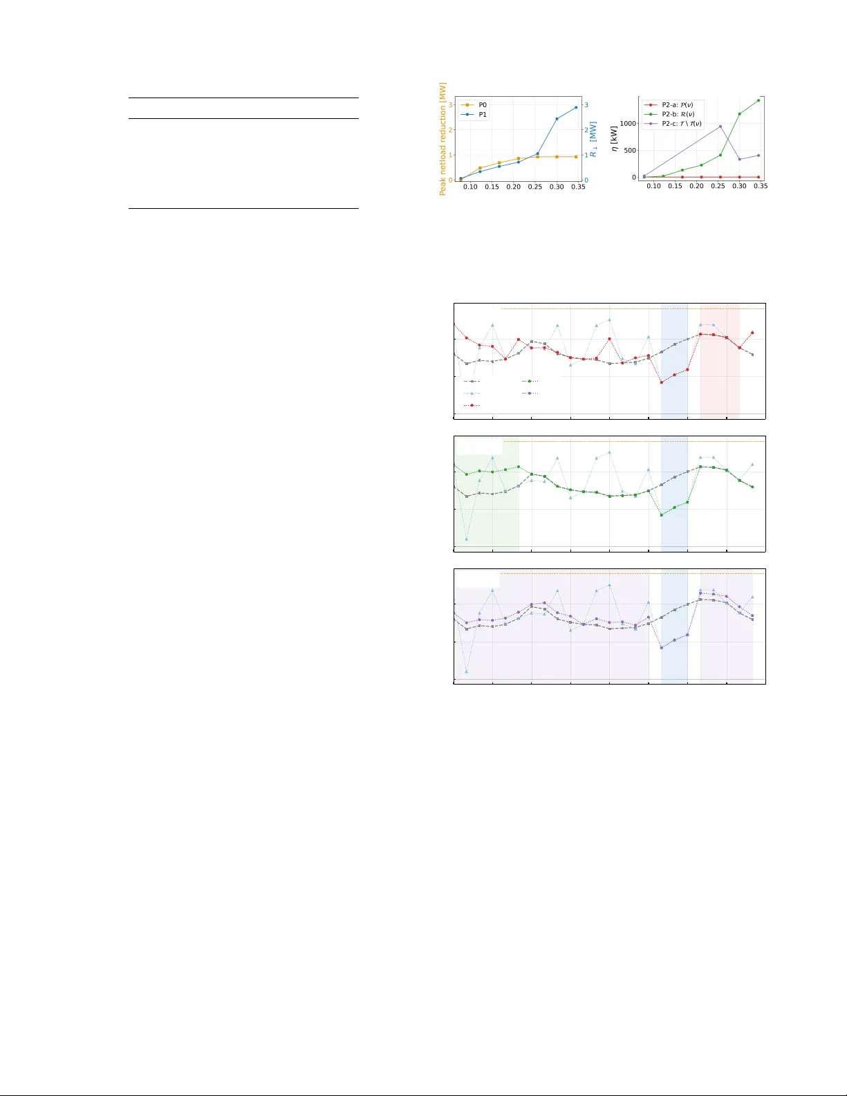
T ime W indo w-Based Netload Range Cost Curves for Coordinated T ransmission and Distrib ution Planning Under Uncertainty Y ujia Li, Alexandre Moreira, Miguel Heleno Lawrence Berkeley National Laboratory , Berkele y , CA, USA yujiali@lbl.gov , AMoreira@lbl.gov , MiguelHeleno@lbl.go v Abstract —Mechanisms to coordinate transmission and distri- bution planning should be regulatory compliant and keep the spheres of DSO and TSO decisions separate, without requiring disclosure of proprietary data or unrealistic computationally expensive T&D co-simulations. The concept of Netload Range Cost Curves (NRCC) has been recently proposed as simple non-in vasive form of coordinating T&D in vestments under distribution netload uncertainty . This paper extends the NRCC concept to accommodate the temporal dimension of the T&D planning process. W e pr opose to compute a hierarch y of certified temporal interface products that repr esent the different levels of flexibility that distribution networks can provide trans- mission grids with at the planning stage. The first product (P1) maps distribution in vestment into scenario-rob ust, per- window ser vice en velopes within which any TSO service call (to modify load within specified bounds) is guaranteed distribution- network-feasible. The second product (P2) adds lexicographic rebound minimization, preser ving P1-optimal service capacity while certifying post-service recov ery under three governance variants with qualitatively distinct rebound-b udget responses. In our numerical results, based on a real distribution feeder , we compare the performance of our proposed time-window- based flexibility products to an atemporal product (P0) that offers a static bound on the aggregate distribution grid netload across all time periods. Our results demonstrate the superiority of our proposed products in properly valuing the benefits of incremental inv estments in storage to allow f or temporal flexibility . Index T erms —Distribution network planning, energy storage, flexibility services, transmission & distribution coordination, uncertainty . N O M E N C L A T U R E Indices and Sets k ∈ K Budget tier inde x and set. t ∈ T T ime-step index; T is the full planning horizon. s ∈ S distributed generation-growth scenario index and scenario set. ν ∈ W Service-window index and window set. T ( ν ) T ime steps belonging to service window ν . R ( ν ) Rebound window for P2-b. P ( ν ) Protected windo w for P2-a. N sub T&D boundary substation nodes. Q Product-variant index set; Q = { a , b , c } . Ω ν Service-call set for windo w ν ; see (3). e Ω ν Stress-screening subset e Ω ν ⊂ Ω ν used in MILP approximation. X pl Planning feasibility set. X op s ( · ) Operational feasibility set under scenario s . X op s,ν ( · ) Service-augmented operational set; see (4). P arameters Γ 0 Least-cost feasible in vestment budget. Γ k T otal inv estment budget at tier k ; Γ k = Γ 0 + ∆Γ k . ∆Γ k NRCC incentiv e increment offered at tier k . W W eighting factor between direct and rev erse peak objectives. Λ D , Λ R Expected peak direct / rev erse netloads. λ D k P0-optimal direct peak cap at tier k . ¯ p 0 t,s Baseline substation netload under scenario s at time t . ρ ν Importance weight assigned to service win- dow ν . β ↓ ν , β ↑ ν Direction scoring factors for downw ard / upward service. θ ↓ ν , θ ↑ ν Sustained duration multipliers [h]; E ↓ ν = θ ↓ ν R ↓ ν , E ↑ ν = θ ↑ ν R ↑ ν . R ⋆ ↓ ν,k , R ⋆ ↑ ν,k P1-optimal power ratings for window ν at tier k . E ⋆ ↓ ν,k , E ⋆ ↑ ν,k P1-optimal energy budgets; E ⋆ ↓ ν,k = θ ↓ ν R ⋆ ↓ ν,k . ∆ t T ime step duration. Decision V ariables u ∈ { 0 , 1 } n u Binary inv estment decision v ector . v ∈ R n v + Continuous sizing decision vector . w s Operational variable vector under scenario s . p sub t,s Substation netload at time t under scenario s . F DN ( · ) Annualized total DN cost function. λ D , λ R Peak direct / re verse substation netload bounds. R ↓ ν , R ↑ ν Downw ard / upward power rating for win- dow ν . E ↓ ν , E ↑ ν Downw ard / upward energy budget for win- dow ν . ξ ↓ t , ξ ↑ t Downw ard / upward service-call trajectory at time t . η W orst-case peak rebound metric. I . I N T R O D U C T I ON Modern power systems planning is ev olving from the clas- sic approach of treating the transmission network in isolation. Behind-the-meter distributed generation are rapidly reshaping the netload profiles seen at transmission and distrib ution (T&D) boundary substations, altering both their magnitude and temporal shape [1]. Since this boundary netload is gov erned by distrib ution-side demand, local constraints, and in vestment decisions of distribution generations, transmission upgrades designed under fixed boundary assumptions will likely lead to either overly conservati ve or insufficient across plausible distrib uted generation and load growth pathways [2]. This coupling creates a practical need for coordinated planning across T&D. In principle, distribution planners can in vest in local upgrades and controllable resources to reshape boundary netload trajectories, potentially deferring transmission reinforcements [2]. In practice, coordination is difficult because TSOs and DSOs operate under different objectiv es, in vestment cycles, model granularities, and data- access constraints [3]. As a result, from a DSO perspecti ve, it remains challenging to provide the transmission planner with netload interface that is simultaneously decision-relev ant for transmission in vestment and credible with respect to distribution feasibility . In addition, to make T&D planning co- ordination realistic and regulatory compliant, it is important to keep the spheres of DSO and TSO decisions separate, without requiring disclosure of proprietary data or computationally expensi ve T&D co-simulations. T o address this challenge, our prior work introduced the concept of netload range cost curves (NRCCs) as a com- pact, non-intrusi ve planning interface for coordinated T&D planning under distributed generation growth uncertainty [3]. The NRCC framework can be seen as a product offered by the DSO to the TSO, in which the DSO provides a menu that pairs peak substation net-load guarantees with the corresponding distribution upgrade costs. This enables the transmission planner to trade off transmission reinforcements against distribution-side in vestments while keeping distribu- tion netw ork models and internal constraints local to the DSO. Howe ver , the current NRCC framework is solely focused on providing peak load guarantees at the substation, which presents three main limitations for T&D planning: first, a bound on the distribution absolute peak cannot capture the temporal structure of transmission stress (i.e., whether that peak is reduced at a time that is critical for the transmis- sion infrastructure); second, when flexibility is provided by energy-limited resources, such as battery storage, there is an energy payback period that is not explicitly allocated to periods that are more conv enient for transmission planning; third, the existing framework offers no mechanism for the DSO to translate distrib ution inv estment into time-specific flexibility commitments that are simultaneously certifiable by the TSO and consistent with internal network constraints. This paper extends the NRCC framework from a peak-only menu to a hierarchy of certified temporal interface products that explicitly characterize both service deliv ery and outside- window rebound behaviour . The contributions are threefold: (i) W e formulate a service-window product (P1) to map a distribution in vestment budget into per -window power and energy ratings within which an y transmission service call is guaranteed distribution-network-feasible under all distributed generation-growth scenarios, moving the T&D interface from T ABLE I: Interface product hierarchy . Prod. Interface guarantee Scope Model P0 Peak/valle y bounds per budget tier T 2 P1 Per-windo w po wer/energy adjust- ments; any TSO call is DN-feasible under all scenarios T ( ν ) 3 P2 P1 ratings locked; rebound mini- mized; variants a/b/c differ in go v- ernance scope variant- dependent 4 a single peak guarantee to a scenario-robust flexibility en- velope that the TSO can query window by window; (ii) W e introduce a lexicographic rebound-minimization stage (P2) that preserves P1-optimal service capacity exactly while minimizing worst-case outside-windo w peak rebound under alternativ e rules. The remainder of this paper is organized as follows. Section II defines the temporal interface product hierarchy and the associated optimization models. Section III describes the solution workflo w . Section IV presents numerical results and discusses implications for fle xibility procurement across T&D at the planning stage. Section V concludes the paper and outlines future directions. I I . T E M P O R A L I N T E R FAC E P R O D UC T S The NRCC framework introduced in [3] in volv es an atem- poral product P0 that offers (from the DSO to the TSO) differ - ent pairs of distribution in vestment b udgets and corresponding peak net load at the point of connection between distribution and transmission grids. This paper extends this framework to a hierarchy of temporal interface products, summarized in T able I. P1 augments P0 with a per-window service en velope defined by a maximum deliv erable power adjustment and an energy budget, within which any TSO service call is guaranteed distribution-network-feasible under all distributed generation-growth scenarios. P2 locks P1-optimal service lev el and further manages post-service rebound. A. Baseline Models in the Original NRCC F ramework 1) Model 1: Scenario-Based Least-Cost Distrib ution Net- work Planning (LCDNP): Model 1 selects the minimum- cost distrib ution netw ork (DN) in vestment plan that remains operationally feasible under all distributed generation gro wth scenarios. Γ 0 = min u , v , w s F DN ( u , v , { w s } s ∈S ) (1a) s.t. ( u , v ) ∈ X pl , (1b) w s ∈ X op s ( u , v ) , ∀ s ∈ S , (1c) u ∈ { 0 , 1 } n u , v ∈ R n v + . (1d) Here u contains binary inv estment decisions, e.g., line recon- ductoring, voltage re gulator and transformer placement, and v contains continuous sizing variables, e.g., storage capacity . V ector w s collects all operational variables under scenario s ∈ S . The objective F DN comprises annualized capital in vestment costs plus a penalty for load shedding, and its optimal value, Γ 0 , is referred to as the least-cost feasible budg et . Let ¯ p 0 t,s denote the substation netload at time t under scenario s in the Model 1 optimal operating schedule { w 0 s } ; this scenario-specific baseline profile is used as the reference for service-window adjustments in Models 3 and 4. 2) Model 2: T ransmission-A ware Distribution Network Planning (T ADNP) (P0): Gi ven an NRCC incenti ve ∆Γ k from the TSO, Model 2 minimizes the worst-case peak netload range at boundary substations across all distributed generation growth scenarios, subject to a total inv estment budget of Γ 0 + ∆Γ k : min u , v , w s ,λ D ,λ R W [ λ D − Λ D ] + + (1 − W )[ λ R − Λ R ] + (2a) s.t. (1b) , (1c) , (1d) , (2b) − λ R ≤ p sub n,t,s ≤ λ D , ∀ n ∈ N sub , t ∈ T , s ∈ S , (2c) λ D , λ R ≥ 0 , (2d) F DN ( u , v , { w s } ) ≤ Γ 0 + ∆Γ k . (2e) Here [ · ] + = max {· , 0 } , W ∈ [0 , 1] is a weighting factor , and Λ D , Λ R are the expected peak direct/rev erse netloads from the deterministic LCDNP under the e xpected scenario. Constraint (2c) enforces that the worst-case peak direct and rev erse substation netloads across all scenarios do not exceed λ D and λ R , which driv e transmission-side reinforcement needs. Solving (2) for each k ∈ K yields one P0 NRCC menu entry: the pair (∆Γ k , [ λ R k , λ D k ]) . Remark 1. The P0 menu should be considered by the trans- mission planner thr ough an NRCC-informed transmission expansion model, one of |K | DSO service options can be se- lected at each boundary substation. That model will optimize the least-cost combination of transmission investments and NRCC pur chases acr oss all boundary nodes. The optimization of the transmission planner decision making is out of the scope of this paper and we focus exclusively on the DSO- side pr oduct construction. B. T emporal NRCC Extension: Service-W indow Pr oducts and Rebound Management 1) Service-W indow Call Set: A service call represents the boundary netload adjustment trajectory that the transmission planner selects within the published service en velope during window ν ∈ W . Let T ( ν ) denote the set of time periods in window ν . The admissible service call set is: Ω ν ( R , E ) := n ( ξ ↓ t , ξ ↑ t ) t ∈T ( ν )    0 ≤ ξ ↓ t ≤ R ↓ ν , P t ξ ↓ t ∆ t ≤ E ↓ ν , 0 ≤ ξ ↑ t ≤ R ↑ ν , P t ξ ↑ t ∆ t ≤ E ↑ ν o . (3) Here ξ ↓ t and ξ ↑ t denote the downw ard and upw ard boundary power adjustments at time t , corresponding to load reduction or local resources’ extra injection/consumption during the service window . The energy budget is parameterized by a sustained duration multiplier: E ↓ ν = θ ↓ ν R ↓ ν and E ↑ ν = θ ↑ ν R ↑ ν , where θ ↓ ν , θ ↑ ν ≥ 0 represent the maximum number of hours the resource can sustain full-po wer deli very , reducing Ω ν to a family indexed by the maximum deliv erable adjustments ( R ↓ ν , R ↑ ν ) alone. 2) Model 3: T emporal NRCC Pr oduct Design (P1): Model 3 co-designs distribution inv estments and service en- velope parameters at b udget tier k : max u , v , w s , R , E X ν ∈W ρ ν  β ↓ ν R ↓ ν + β ↑ ν R ↑ ν  (4a) s.t. ( u , v ) ∈ X pl , (4b) F DN ( u , v , { w s } ) ≤ Γ 0 + ∆Γ k , (4c) u ∈ { 0 , 1 } n u , v ∈ R n v + . (4d) ∀ ν ∈ W , s ∈ S , ( ξ ↓ , ξ ↑ ) ∈ Ω ν ( R , E ) : ∃ w s ∈ X op s,ν  u , v ; ξ ↓ , ξ ↑  , (4e) where: X op s,ν ( · ) :=    w s : w s ∈ X op s ( u , v ) , p sub t,s = ¯ p 0 t,s − ξ ↓ t + ξ ↑ t , ∀ t ∈ T ( ν ) , − λ R k ≤ p sub t,s ≤ λ D k , ∀ t ∈ T \ T ( ν )    . The objecti ve (4a) maximizes the weighted sum of de- liv erable adjustments across all windows. Constraints (4b)– (4c) enforce planning feasibility and the in vestment budget. Constraint (4e) is the deliverability requirement: for ev ery admissible service call and every scenario, there must exist a DN-feasible operating schedule implementing the requested boundary adjustment. Outside the service windo w , X op s,ν en- forces − λ R k ≤ p sub t,s ≤ λ D k , where λ D k and λ R k are the P0- optimal bounds at tier k , ensuring that the P1 product does not worsen outside-window transmission conditions relativ e to the P0 baseline. In its exact form, constraint (4e) requires verification ov er all calls in Ω ν . 3) Model 4: Rebound-A ware Refinement (P2): For energy- limited flexibility resources, service within T ( ν ) induces en- ergy reco very outside the windo w that can create uncontrolled netload excursions if left ungov erned. Model 4 performs a lexicographic second stage gi ven the P1-optimal deliv erable adjustments and energy budgets ( R ⋆ ↓ ν,k , R ⋆ ↑ ν,k , E ⋆ ↓ ν,k , E ⋆ ↑ ν,k ) for in vestment budget tier k from Model 3: it preserves each per-windo w rating at its P1-optimal level and minimizes the worst-case peak rebound η : min u , v , w s , R , E , η η (5a) s.t. F DN ( u , v , { w s } ) ≤ Γ 0 + ∆Γ k , (5b) u ∈ { 0 , 1 } n u , v ∈ R n v + . (5c) R ↓ ν ≥ R ⋆ ↓ ν,k , R ↑ ν ≥ R ⋆ ↑ ν,k , E ↓ ν ≥ E ⋆ ↓ ν,k , E ↑ ν ≥ E ⋆ ↑ ν,k , ∀ ν ∈ W , (5d) ∀ ν ∈ W , s ∈ S , ( ξ ↓ , ξ ↑ ) ∈ Ω ν ( R , E ) : ∃ w s ∈ Y q s,ν  u , v ; ξ ↓ , ξ ↑ ; η  . (5e) Here q ∈ { a , b , c } index es the product variant ( q = c is a special case of a ; see below) and Y q s,ν is the rebound- augmented recourse set. Constraint (5d) is the P1-capacity floor : it pins the minimum deliverable adjustments and en- ergy budgets at their P1-optimal values so that Model 4 cannot sacrifice service capacity in pursuit of lo wer rebound. Critically , Model 4 re-optimizes all in vestments from scratch under the same budget Γ k , inheriting only the service lev el from Model 3; this allows a different resource portfolio to be selected if it achiev es lower rebound at the same service level. Constraint (5e) requires, for ev ery admissible service call and ev ery scenario, the existence of a DN-feasible schedule that implements the boundary adjustment and obeys the outside- window governance rule of v ariant q . P2-a (protected windo w P ( ν ) , q = a ) defines: Y a s,ν ( · ) := n w s ∈ X op s,ν ( · ) :   p sub t,s − ¯ p 0 t,s   ≤ η , ∀ t ∈ P ( ν ) , − λ R k ≤ p sub t,s ≤ λ D k , ∀ t ∈ T \ ( T ( ν ) ∪ P ( ν )) o . (5e) P2-b (rebound windo w R ( ν ) , q = b ) defines: Y b s,ν ( · ) := n w s ∈ X op s,ν ( · ) :   p sub t,s − ¯ p 0 t,s   ≤ η , ∀ t ∈ R ( ν ) , p sub t,s = ¯ p 0 t,s , ∀ t ∈ T \ ( T ( ν ) ∪ R ( ν )) o . (5f) Constraints (5a)–(5e) using Y a s,ν and Y b s,ν constitute Model 4- a and Model 4-b , respecti vely . The two v ariants reflect complementary positions along a flexibility-predictability trade-off. P2-a designates P ( ν ) as a pr otected window where post-service ener gy recovery is bounded by η , while hours outside T ( ν ) ∪ P ( ν ) retain the P1 peak-cap guarantee. This suits applications where the TSO must av oid new peak violations following service but can tolerate P1-level behavior else where. On the other hand, P2-b designates R ( ν ) as the sole window where ener gy recov ery may deviate from baseline, locking all remaining hours to the baseline netload exactly and providing the TSO with full boundary predictability outside T ( ν ) ∪ R ( ν ) , at the cost of a potentially larger η within that slot. Note that P2-a subsumes a global rebound en velope as a special case when P ( ν ) = T \ T ( ν ) ; this variant, denoted P2-c , is ev aluated in the case study (Section IV). Remark 2. Unlike P0, which publishes a single peak bound per substation, P1 and P2 certify a window-specific flexibility en velope within which the TSO can fr eely shape its service r equests accor ding to transmission-le vel needs. This supports mor e tar geted pr ocurement, e.g., calling service only during coincident str ess hours, and can be inte grated into TSO-side models that co-optimize transmission in vestments and DSO contracts, which will be fully pr esented in our futur e work. I I I . S O L U T I O N M E T H O D A N D W O R K FL OW In the previous section, constraints (4e) and (5e) require verifying deliverability over all calls in Ω ν , all scenarios s ∈ S , and all windows ν ∈ W . The full formulation of the operational and planning feasibility sets X op s and X pl , including linearized DistFlow constraints, distributed generation models, and in vestment cost functions, follows [3]. In this paper , we adopt a str ess-scr eening approximation that replaces the deli verability check over all admissible calls in Ω ν with a finite set e Ω ν ⊂ Ω ν of representative patterns, enabling direct MILP solution; the exact verification procedure is deferred to future work. A. Str ess-Call Screening Set For each windo w ν with |T ( ν ) | = H steps, let τ ↓ ν := ⌊ θ ↓ ν / ∆ t ⌋ . Four canonical downward patterns m ∈ M = Algorithm 1: T emporal NRCC product construction Input : Feasibility sets X pl , {X op s } s ∈S ; budget tiers { ∆Γ k } k ∈K ; window parameters ( θ ↓ / ↑ ν , ρ ν , β ↓ / ↑ ν ) ν ∈W ; rebound windo ws P ( ν ) , R ( ν ) . Output: Per tier k : P0 bounds ( λ D k , λ R k ) ; P1 en velope ( R ⋆ ↓ ν,k , R ⋆ ↑ ν,k , E ⋆ ↓ ν,k , E ⋆ ↑ ν,k ) ν ∈W ; P2 rebound bounds η k,q , q ∈ { a , b , c } . Solve (1); record Γ 0 and ¯ p 0 t,s , ∀ t, s for k ∈ K do P0: atemporal NRCC Solve (2) at Γ 0 + ∆Γ k ; record λ D k , λ R k P1: service-window en velope Build e Ω ν via four stress patterns, ∀ ν ∈ W Solve (4) ov er e Ω ν × S ; record ( R ⋆ ↓ ν,k , R ⋆ ↑ ν,k , E ⋆ ↓ ν,k , E ⋆ ↑ ν,k ) , ∀ ν P2: rebound-awar e refinement for q ∈ { a , b , c } do Solve (5)- q with floors (5d); record η k,q end end { base , sust , start , end } are defined as ξ ↓ ,m t :=              0 m = base , θ ↓ ν R ↓ ν H ∆ t m = sust , R ↓ ν · 1 [ t ≤ t τ ↓ ν ] m = start , R ↓ ν · 1 [ t ≥ t H − τ ↓ ν +1 ] m = end , (6) where 1 [ · ] is the indicator function. Upward patterns are defined symmetrically by replacing ↓ with ↑ . T ogether , these patterns stress the service en velope from complementary power –energy angles: base provides a no-call reference; sust spreads the full energy budget uniformly at reduced power , stressing the energy-to-po wer ratio of the distribution network’ s fle xibility resources; start and end concentrate full-power calls at the beginning and end of the window , respectiv ely , testing whether the network can sustain delivery after early depletion or enter service with sufficient resource headroom. The screening set is thus: e Ω ν ( R , E ) :=  ( ξ ↓ ,m , ξ ↑ ,m ′ ) | m, m ′ ∈ M  ∩ Ω ν ( R , E ) (7) and deliverability is enforced for each element of e Ω ν across all scenarios s ∈ S and windo ws ν ∈ W , yielding | e Ω ν | · |S | feasibility blocks per windo w per budget tier . B. Pr oduct Construction Pr ocedure Algorithm 1 constructs the full product hierarchy by sweeping the b udget le vels { ∆Γ k } and solving, at each tier , Models 1–4 in sequence. 1) Baseline and P0 (Models 1–2): Model 1 is solved once to obtain the least-cost budget Γ 0 and the baseline netload profiles ¯ p 0 t,s . For each tier k , Model 2 is then solved at Γ 0 + ∆Γ k to obtain the P0 bounds ( λ D k , λ R k ) , which serve as the outside-window guarantees in all subsequent stages. 2) P1 Construction (Model 3): F or each tier ∆Γ k , the deliv erability constraint (4e) is replaced by finite feasibility blocks over e Ω ν × S , appended directly to the inv estment T ABLE II: Case study parameters. Parameter V alue Candidate storage duration 2 h Service window T ( ν ) Hours 16–18 Duration multiplier θ ↓ 2 h P2-a protected windo w P ( ν ) Hours 19–22 P2-b rebound windo w R ( ν ) Hours 0–5 P2-c rebound windo w T \ T ( ν ) optimization as a single MILP . The solution yields the per- window service en velope ( R ⋆ ↓ ν,k , E ⋆ ↓ ν,k , R ⋆ ↑ ν,k , E ⋆ ↑ ν,k ) ν ∈W , which serves as the P1-capacity floor (5d) for P2. 3) P2 Construction (Model 4): Giv en the P1-optimal en- velope, Model 4 is solved once per v ariant q ∈ { a , b , c } . The P1-capacity floor (5d) pins each window’ s deliv erable adjustments and energy budgets at their P1-optimal values, reducing the second-stage problem to minimizing η under the chosen outside-windo w governance rule (5e) or (5f). I V . C A S E S T U DY A N D R E S U LT S A. T est System and Setup The framework is applied to a representativ e feeder ( p8udt1252-p8uhs6_1247x , located in San Francisco, CA) from the SMAR T -DS synthetic distrib ution dataset [4]. The feeder has 65 buses and 60 lines, and has 5/5/1 candidate lines/storage units/voltage re gulators for reinforcement or installation, respecti vely . Parameters and costs associated with candidate line reinforcements, storage systems, and VRs on the distribution network side are extracted from [5], [6]. Long-term netload uncertainty is generated based on the same procedure in [3] and reduced to 3 scenarios cov ering 3 representativ e days. Combined with the four canonical stress- call patterns from Algorithm 1, this yields 12 feasibility blocks per window per b udget le vel. For bre vity , the case study considers a single downw ard service window ( R ↑ = 0 ); upward service windows are left for future work. The service window T ( ν ) covers hours 16–19, when the ev ening demand ramp after distributed generation subsides produces the highest and most temporally concentrated net- load across all scenarios, making it the most likely target for TSO-initiated flexibility calls and the most demanding test of P1 deli verability . The protected window P ( ν ) (hours 20– 23) immediately follows service, and the designated rebound window R ( ν ) (hours 0–5) targets the overnight low-stress slot, together covering the full post-service reco very cycle that P2 governs. T able II summarizes the remaining parameters. B. P0 and P1 Results Fig. 1(a) reports the P0 peak cap λ D k and P1 downw ard rating R ↓ versus incremental budget ∆Γ . The cost-optimal baseline yields Γ 0 ≈ $77 , 859 /yr . P0 peak reduction satu- rates beyond ∆Γ ≈ 178 k/yr , with the cap declining from 6,537 kW to 5,615 kW ( ∼ 14%) as scenario-driv en netload uncertainty is progressivel y eliminated. In contrast, R ↓ grows throughout, reaching ∼ 2,900 kW at the highest tier, dri ven by storage in vestment. The di vergence of the two curves beyond saturation re veals that b udget increments yielding ne gligible peak reduction can still unlock substantial temporal flexibility , Additional budget [M$/yr] (a) P0 peak cap and P1 R ↓ . Additional budget [M$/yr] (b) P2 rebound η vs. budget. Fig. 1: P0 peak netload reduction, P1 service capability , and P2 rebound metric across budget tiers. 0 2 4 Netload [MW]  ( ν )  ( ν ) (a) P2-a Baseline P1 P2-a P2-b P2-c 0 2 4 Netload [MW]  ( ν )  ( ν ) 5.6 MW (b) P2-b 0 3 6 9 12 15 18 21 24 Hour of day 0 2 4 Netload [MW]  ( ν )  \  ( ν ) 5.6 MW (c) P2-c Fig. 2: Substation netload profiles under sustained do wn-call for P2 variants at reference tier . Shaded regions mark service window T ( ν ) and v ariant-specific recovery windo ws. which is a value that the atemporal P0 interface alone cannot capture. T wo structural features of the P1 curve merit attention. First, R ↓ grows approximately linearly up to ∆Γ ≈ 134 k/yr ( R ↓ ≈ 710 kW), consistent with storage-dominated in- vestment at a roughly constant marginal cost. Second, a pronounced jump occurs near ∆Γ ≈ 222 k/yr, where R ↓ rises steeply from ∼ 1 , 050 kW to ∼ 2 , 440 kW . This step change reflects a discrete inv estment regime transition, where additional storage capacity becomes accessible only after upstream line reinforcements are activ ated, and underscores that flexibility supply is not a smooth function of budget on networks with discrete in vestment options. C. P2 Results: Rebound Response Fig. 1(b) shows η versus ∆Γ for all three P2 variants. In addition to P2-a and P2-b, we e valuate P2-c, a global rebound variant that bounds deviation from baseline over all non-service hours T \ T ( ν ) without designating a specific recov ery window . The three variants e xhibit qualitativ ely different budget responses, showing that governance design rather than budget allocation is the primary determinant of rebound scaling beha vior . P2-a maintains η = 0 across all budget le vels. Under the P2-a gov ernance rule, storage is not required to complete recharge within P ( ν ) ; hours outside T ( ν ) ∪ P ( ν ) remain subject only to the P0 peak cap, providing ample time for storage to recharge without deviating from baseline during the protected windo w . Consequently , P ( ν ) experiences zero netload deviation regardless of how much energy was dis- charged during service, and η = 0 holds e ven at the highest tier where R ↓ ≈ 2 , 900 kW . P2-b shows monotonically increasing η . As storage in vest- ment enables greater R ↓ , more energy must be recov ered within the ov ernight slot R ( ν ) (hours 0–5), progressively saturating its limited headroom. At the highest budget tier, η exceeds 1,400 kW , revealing a fundamental tension in the P2- b design: stronger service capability directly worsens rebound concentration. P2-c exhibits non-monotone behavior , with η peaking near ∼ 940 kW at intermediate b udgets before declining. The initial rise parallels P2-b as gro wing service ener gy increases total recovery volume. At higher budgets, howe ver , expanded storage and network capacity enable more effecti ve temporal spreading, reducing the worst-case per-hour de viation. D. Load Pr ofile Analysis Fig. 2 overlays representative substation netload profiles for the sustained down-call scenario. P1 is included as a reference: while it deliv ers the same service-window do wn- ramp as all P2 variants, its outside-window profile fluctuates freely as storage recharges without any rebound gov ernance, producing large uncontrolled deviations from baseline. The P2 variants each suppress this behavior dif ferently . Under P2-a , the profile within P ( ν ) tracks baseline closely , consistent with η = 0 , while hours outside T ( ν ) ∪ P ( ν ) retain P1-lev el freedom below the peak cap. The TSO observes intended service follo wed by seamless return to baseline in the protected window . Under P2-b , all hours outside T ( ν ) ∪ R ( ν ) adhere strictly to baseline, eliminating the uncontrolled fluctuations visible in P1 everywhere except the ov ernight slot (hours 0–5), where ener gy recov ery is visibly concentrated. This sharp concentration directly explains the monotonically growing η : the entire post-service energy debt is compressed into a windo w whose headroom does not scale with in vestment. Under P2-c , the profile tracks baseline throughout all non-service hours with small uniform devi- ations, substantially smoothing the P1 fluctuations without designating a specific recov ery slot. The three variants thus span a flexibility–predictability spectrum. The choice among them depends on whether the TSO prioritizes zero post-service deviation (P2-a), full-day baseline adherence outside a designated slot (P2-b), or global worst-case deviation minimization (P2-c). E. Discussion The results re veal three implications for temporal fle xibility product design. First, the P0 and P1 curves div erge at higher budget tiers, nonetheless, confirming that incremental in vest- ments in storage can be better valued by time-window-based products by considering temporal flexibility . Second, rebound behavior is gov erned by contract design rather than budget: despite sharing the same P1-optimal service capacity , the three P2 variants exhibit qualitati vely distinct η -budget rela- tionships, confirming that a rebound bound is meaningful only when paired with its governance structure. Third, the choice among P2 variants inv olves a fundamental trade-off: P2-a offers the strongest rebound guarantee with moderate outside- window freedom, P2-b provides full baseline predictability at the cost of gro wing rebound concentration, and P2-c minimizes peak hourly de viation globally without protected or rebound window-specific commitments. The appropriate variant depends on the TSO’ s operational priorities. V . C O N C L U S I O N This paper proposed a hierarchy of certified temporal flexibility products (P0, P1, P2) within the NRCC framew ork for TSO–DSO coordinated planning. P1 maps distribution in vestment into scenario-robust service-window en velopes; P2 adds lexicographic rebound minimization with three gov- ernance variants that exhibit qualitativ ely distinct budget– rebound responses, confirming that rebound guarantees are meaningful only when specified jointly with gov ernance rules. Future work will replace the stress-screening approxima- tion with the full deliverability verification procedure for stronger robustness guarantees, integrate the P1 and P2 products into the TSO-side portfolio selection model to quantify the transmission planning value of rebound-certified flexibility , and validate the proposed framework across multi- substation feeders with div erse load shapes to characterize the conditions under which each governance v ariant is most advantageous. R E F E R E N C E S [1] G. Mu ˜ noz-Delgado, J. Contreras, J. M. Arroyo, A. Sanchez de la Nieta, and M. Gibescu, “Integrated transmission and distrib ution system expansion planning under uncertainty , ” IEEE T ransactions on Smart Grid , vol. 12, no. 5, pp. 4113–4125, 2021. [2] F . Capitanescu, “Barriers and insights to compute multi-period cost curves of acti ve power aggregated flexibility from distribution systems for tso-dso coordination, ” IEEE Tr ansactions on P ower Systems , vol. 40, no. 6, pp. 5410–5421, 2025. [3] Y . Li, S. C ´ ordov a, A. Moreira, and M. Heleno, “Netload range cost curves for coordinated transmission-distribution planning under der growth uncertainty , ” IEEE T ransactions on Energy Markets, P olicy and Re gulation , pp. 1–15, 2025. [4] National Renewable Energy Laboratory (NREL), “SMAR T -DS synthetic electrical network data OpenDSS models for SFO, GSO, and A US, ” 2020. [Online]. A vailable: https://data.openei.org/submissions/2981 [5] W . H. Kersting, “Distribution system modeling and analysis, ” in Electric power generation, transmission, and distribution . CRC press, 2018, pp. 26–1. [6] National Renewable Energy Laboratory (NREL), “2019 distribution system upgrade unit cost database current version, ” 2019. [Online]. A vailable: https://data.nrel.gov/submissions/101