Koopman Operator Identification of Model Parameter Trajectories for Temporal Domain Generalization (KOMET)
Parametric models deployed in non-stationary environments degrade as the underlying data distribution evolves over time (a phenomenon known as temporal domain drift). In the current work, we present KOMET (Koopman Operator identification of Model par…
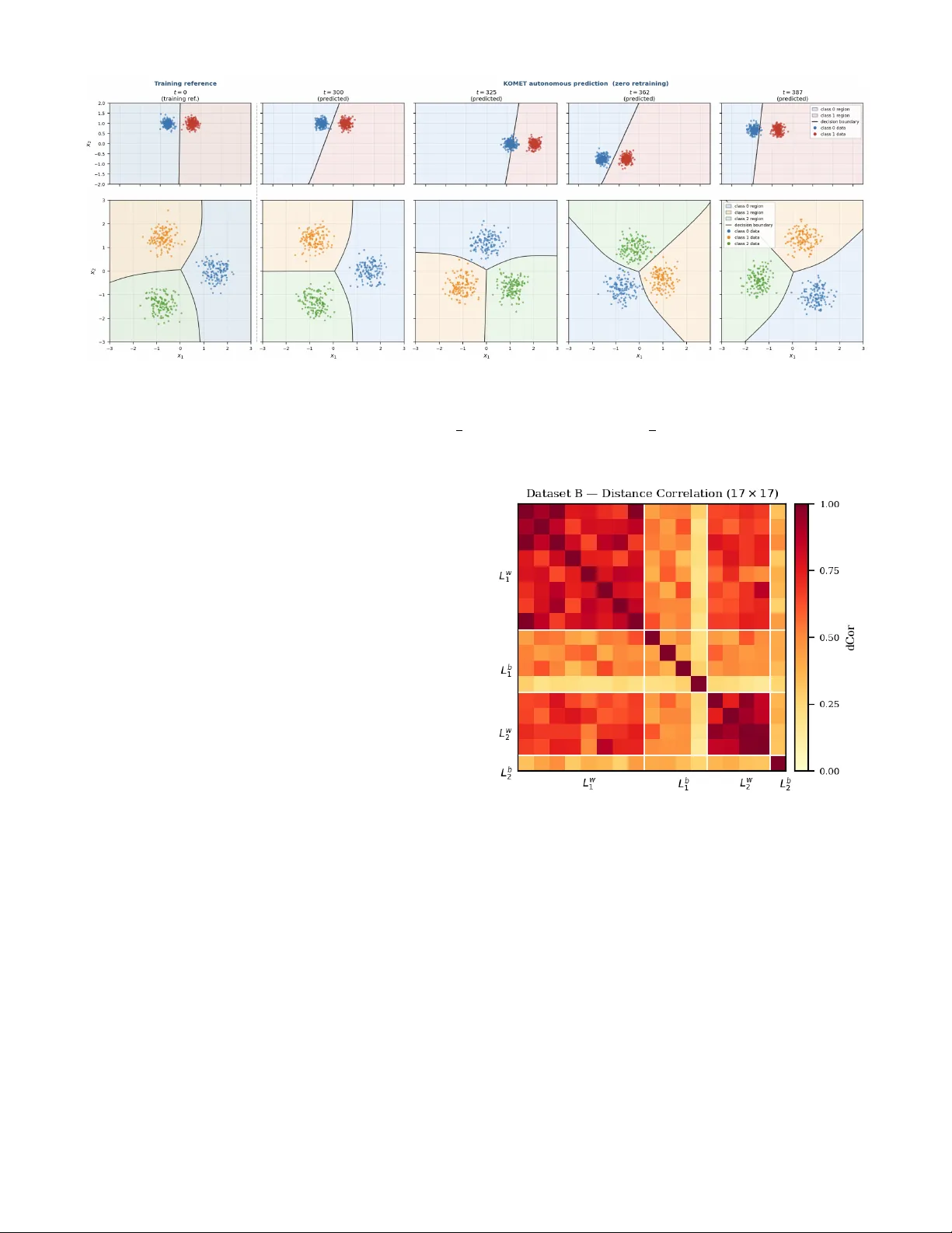
Authors: R, y C. Hoover, Jacob James
K oopman Operator Identification of Model Parameter T rajectories f or T emporal Domain Generalization (K OMET) Randy C. Hoov er , Jacob James, Paul May , and K yle Caudle Abstract — Parametric models deployed in non-stationary en- vironments degrade as the underlying data distribution evolv es over time (a phenomenon known as temporal domain drift). In the current work, we present KOMET (Koopman Operator identification of Model parameter Evolution under T emporal drift), a model-agnostic, data-driven framework that treats the sequence of trained parameter vectors as the trajectory of a nonlinear dynamical system and identifies its governing linear operator via Extended Dynamic Mode Decomposition (EDMD). A warm-start sequential training protocol enf orces parameter - trajectory smoothness, and a Fourier -augmented observ able dictionary exploits the periodic structure inherent in many real- world distribution drifts. Once identified, K OMET’ s K oopman operator predicts future parameter trajectories autonomously , without access to future labeled data, enabling zero-r etraining adaptation at deployment. Evaluated on six datasets spanning rotating, oscillating, and expanding distribution geometries, K OMET achieves mean autonomous-rollout accuracies between 0.981 and 1.000 over 100 held-out time steps. Spectral and cou- pling analyses further reveal interpretable dynamical structur e consistent with the geometry of the drifting decision boundary . I . I N T RO D U C T I O N Parametric models deployed in real-world environments routinely encounter data whose statistical properties drift ov er time, a phenomena collecti vely described as distribu- tion drift or concept drift [1], [2]. The machine-learning community has addressed this primarily through Domain Generalization (DG), where they train on source domains and generalize to an unseen targets [3], [4], using techniques such as domain-adversarial learning [5], in variant risk mini- mization [6], transfer learning [7], and distributionally robust optimization [8]. These methods share a critical limitation because domains are treated as unordered, so temporal structure carries no predictiv e information about the future. T emporal Domain Gener alization (TDG) removes this restriction by lev eraging dynamical systems theory to model the ordered domain sequence as a time series [9]. W ithin TDG, the central question is how to represent and exploit the dynamics of change. DRAIN [10] represents each model snapshot as a dynamic graph and trains a Bayesian recurrent generator to extrapolate full weight sets to the next unseen domain. K oodos [11] extends this to continuous time, con- structing a neural-ODE K oopman embedding over the joint R. C. Hoover and P . May are with the Department of Electrical Engi- neering and Computer Science (EECS), South Dakota Mines, Rapid City , SD 57702, USA { randy.hoover, paul.may } @sdsmt.edu J. James is a Ph.D. student in the Data Science and Engineering Program within EECS, South Dakota Mines, Rapid City , SD 57702, USA jacob.james@mines.sdsmt.edu K. Caudle is with the Department of Mathematics, South Dakota Mines, Rapid City , SD 57702, USA kyle.caudle@sdsmt.edu space of distributions and parameters. Complementary ap- proaches track ev olving normalization statistics [12], enforce continuous inv ariance [13], or apply incremental online- learning strategies [14], [15]. A concurrent complementary approach, SLA TE [16], addresses the same TDG setting via a low-rank batch-smoothing factorization of the full parameter trajectory , using cubic B-spline temporal bases and an AR(1) Gauss-Markov prior to enforce smoothness without recur- rence or sequential rollout. The current work and SLA TE thus target the same problem from orthogonal angles, in verse dynamical-systems identification versus structured trajectory smoothing. A parallel thread has matured in dynamical systems via K oopman operator theory [17], [18]. The K oopman operator is an infinite-dimensional linear operator gov erning the evo- lution of observable functions of a nonlinear system, enabling exact global linearization of complex dynamics. Practical finite-dimensional approximations are computed by Extended Dynamic Mode Decomposition (EDMD) [19], which fits a linear operator in a user -specified observable dictionary where its eigen values directly encode dominant frequencies and decay rates [20]. Deep learning has been combined with EDMD to learn dictionaries automatically [21], [22], and the connection to neural ODEs has been clarified [23]. Despite rapid advances in both TDG and K oopman meth- ods, a fundamental perspectiv e is absent: treating the se- quence of trained parameter vectors themselves as a nonlin- ear dynamical system and performing rigorous system identi- fication on observed trajectories. DRAIN and K oodos answer a forward prediction question which is, given a domain history , predict weights for the next domain, howe ver , neither recov ers the mechanistic law governing how parameters ev olve, nor e xposes the spectral modes and coupling structure that enable analytical characterization of the drift. A. Contributions of the Curr ent W ork W e propose KOMET (Koopman identification of Model parameter Evolution under Temporal drift), a model-agnostic pipeline for post-hoc dynamical-systems identification of parametric model parameter trajectories under periodic distri- bution drift. KOMET treats the model itself as an underlying dynamical system and is complementary to DRAIN and K oodos in that, they solve a forward prediction problem inside a joint training loop, K OMET solves an in verse iden- tification problem on observed model parameter trajectories, requiring no architectural modification and no distributional model of the drift. Specifically , the current paper provides the follo wing contributions: 1) EDMD Koopman identification and autonomous r oll- out: A physics-informed dictionary (Fourier harmonics at the known drift period plus polynomial terms in the PCA- whitened state) is used to fit a low-dimensional Koopman operator via EDMD, then rolled out autonomously over the held-out horizon without access to future labeled training data. 2) Exact forwar d-pr ediction performance: On all datasets satisfying the periodicity assumption, autonomous prediction matches the fully-retrained upper bound (mean accuracy 0 . 981 – 1 . 000 , zero timesteps belo w 90% over 100 held-out steps) across binary and three-class tasks spanning di verse drift geometries. 3) Interpr etable spectral and coupling analysis: The K oopman eigenspectrum encodes drift periodicity and attrac- tor damping. Distance correlation and transfer entropy analy- ses expose layer-wise coupling demonstrating that first-layer weights dominate under simple drift (TE ratio 1 . 95 × layer L1 → layer L2) and become bidirectional as classification difficulty increases, consistent with harder representational demands at Layer 1. 4) W arm-start training with Adam moment continuity: Parameters are trained sequentially across T timesteps, warm-starting both weights and the full Adam state across transitions. A temporal smoothness penalty λ s ∥ θ t − ˆ θ t − 1 ∥ 2 , where ˆ θ is a fixed estimate of the the parameter θ , is added to the loss to prevent trajectory discontinuities. For softmax networks, ℓ 2 weight decay counteracts scale-in variance that would otherwise dri ve unbounded weight growth and violate the Koopman periodicity assumption and stability enforce- ment through spectral reprojection. T ogether these reduce mean epochs-to-con ver gence by 9 -fold and produce smooth, K oopman-amenable weight trajectories. The remainder of this paper is org anized as follows: Sec- tion II provides some background material and mathematical preliminaries required to understand the K OMET pipeline. Section III outlines the entire KOMET approach and the two phase pipeline. Section IV outlines the datasets used for experimental analysis within the K OMET framework and presents experimental results compared to baseline retraining or frozen-start methods. Finally , Section V outlines some conclusions and provides some promising future directions to explore. I I . B AC K G R O U N D & M A T H E M A T I C A L P R E L I M I NA R I E S A. K oopman Operator Theory Consider a discrete-time autonomous dynamical system θ t +1 = F ( θ t ) , θ t ∈ M ⊆ R n θ , (1) where F : M → M is in general nonlinear . The Koopman operator K [17] is an infinite-dimensional linear operator that acts on scalar observable functions g : M → R according to K g = g ◦ F . (2) Linearity is the key property because ev en when F is nonlinear , every observable ev olves linearly under K . The tradeoff is dimensionality , i.e., the operator acts on a function space rather than on M directly . If a finite-dimensional K oopman-in variant subspace exists, spanned by observables { ψ 1 , . . . , ψ N } , then the dynamics of the lifted state vector ψ ( θ ) = [ ψ 1 ( θ ) , . . . , ψ N ( θ )] ⊤ are governed exactly by a finite matrix A ∈ R N × N such that ψ ( θ t +1 ) = A ψ ( θ t ) . (3) The eigenv alues { λ i } of A , the Koopman eigen values , en- code temporal frequencies and gro wth rates of the underlying dynamics. F or a stable autonomous system the spectral radius ρ ( A ) ≤ 1 ensures that autonomous rollouts (i.e., forward propagation) of (3) are forward in variant. Mezi ´ c [18] estab- lished the spectral foundations, Brunton et al. [20] provide a comprehensiv e modern revie w , and the Koopman spectral approach to control is present in [24]. B. Extended Dynamic Mode Decomposition Extended Dynamic Mode Decomposition (EDMD) [19] fits a finite-dimensional approximation of A from data. Giv en a trajectory { θ t } T t =0 , form the snapshot matrices Ψ − = ψ ( θ 0 ) · · · ψ ( θ T − 1 ) , Ψ + = ψ ( θ 1 ) · · · ψ ( θ T ) , (4) and solve the least-squares problem A = arg min A ′ Ψ + − A ′ Ψ − 2 F = Ψ + Ψ † − , (5) where ( · ) † denotes the Moore–Penrose pseudoinv erse. Under mild ergodicity conditions, EDMD con verges to the true K oopman matrix as T → ∞ for a fixed dictionary [19], [20]. Practical issues in long-horizon predictions, including spectral pollution and drift off the state manifold, motiv ate the reprojection strategies studied in [25], [26] to enforce the spectral radius condition ρ ( A ) ≤ 1 . W e note that deep learning extensions have also been established to learn ψ from data [21], ho wev er , when the dominant drift frequencies are kno wn a priori (as in the setting explored here) an explicit physics-informed dictionary is more interpretable while reducing complexity . C. P arameter Coupling and Dimensionality Reduction EDMD scales as O ( N 2 T ) in the observable dimension N . For a network with n θ parameters, a nai ve choice of ψ = [ z , sin( k ωt ) , cos( k ω t )] gi ves N = n θ + 2 K + 1 observ- ables. Ho we ver , the weight trajectory { θ t } is not entirely unstructured due to shared optimization dynamics and the model’ s coupling structure which impose strong statistical dependencies among parameters. W e quantify these using two complementary measures. Distance corr elation [27] (dCor) measures both linear and nonlinear dependence between any two random vectors in [0 , 1] with 0 implying no dependence and 1 implying they are completely dependent. For a pair ( X , Y ) , R ( X, Y ) = s d Co v 2 ( X, Y ) p d V ar( X ) d V ar( Y ) , (6) where the distance cov ariance is computed via doubly- centered Euclidean distance matrices. Unlike Pearson corre- lation, R ( X , Y ) = 0 if and only if X and Y are statistically independent. T r ansfer entropy [28] (TE) quantifies directed information flow from X to Y : TE( X → Y ) = H ( Y t | Y t − 1 ) − H ( Y t | Y t − 1 , X t − 1 ) , (7) where H ( · | · ) is conditional Shannon entropy . TE is asymmetric in that TE( X → Y ) = TE( Y → X ) in general, making it sensitive to the dir ection of information transfer across model layers. Across our experimental datasets (Section IV), dCor analysis re veals that 26–57% of parameter pairs co-vary strongly ( R > 0 . 5 ), and TE analysis shows predominantly bidirectional inter-layer coupling. High coupling means the effecti ve degrees of freedom in the trajectory are far fewer than n θ . This motiv ates projecting onto the leading principal components (PCA whitening) before constructing the EDMD dictionary . W e demonstrate that retaining components that explain ≥ 99 . 5% of trajectory v ariance compresses the n θ -dimensional weight space to a p ≪ n θ dimensional subspace while preserving the structure the K oopman fit needs to be accurate. W e note that PCA is used purely as a dimensionality reduction step for EDMD and refer to the projected coordinates as z ∈ R p . I I I . T H E K O M E T P I P E L I N E K OMET is a tw o-phase pipeline, illustrated in Fig. 1. The pipeline is model-agnostic in that Phase 1 requires only that the base learner f θ be a differentiable parametric model trained by a momentum-based gradient optimizer; and Phase 2 operates solely on the resulting weight trajectory and is indifferent to the model’ s functional form. Candidate base learners include logistic regressors, kernel SVMs with differentiable kernels, and deep neural networks of arbitrary architecture. Here we instantiate f θ as a small feedforward multi-layer perceptron (MLP) for concreteness and to pro- vide reproducible benchmarks on controlled synthetic tasks (Section IV). A. Base Learner Instantiation For the experiments reported here we instantiate f θ as a relativ ely simple two-layer feedforward network ˆ y = σ ( W 2 σ ( W 1 x + b 1 ) + b 2 ) , (8) with σ ( z ) = (1 + e − z ) − 1 . For binary classification ( d = 2 inputs, h = 4 hidden units, c = 1 output) this gives n θ = 17 parameters; and for c -class problems ( c = 3 ) a linear-softmax output head giv es n θ = 27 parameters. These small architectures are chosen deliberately because they are large enough to solve the task at hand yet small enough for their weight-space dynamics to be fully interpretable, making them ideal for a first dynamical-systems analysis of the kind K OMET provides. At each timestep t = 0 , 1 , . . . , T train a fresh mini-batch D t is drawn from the drifting distribution. The network is trained by minimizing L t ( θ ) = L task ( θ ; D t ) | {z } BCE or CE + λ s ∥ θ − ˆ θ t − 1 ∥ 2 + λ wd 2 ∥ θ ∥ 2 , (9) where θ t − 1 remains stationary from the prior training cycle, λ s is a smoothing hyperparameter , λ wd controls weight and the hyperparameters v ary by classification task as outlined below Setting L task λ s λ wd Binary (A–C) BCE 10 − 4 0 3-class (D–F) CE 10 − 4 10 − 3 The current hyperparameter selection is a necessary con- dition for Koopman compatibility . Binary networks use a sigmoid output, which means that once σ ( h ) ≈ 1 the gradient σ ( h )(1 − σ ( h )) ≈ 0 , providing an implicit weight-magnitude bound, so λ wd = 0 suffic es. Multi-class networks use soft- max, which has an exact scale inv ariance, i.e., multiplying all output logits by c > 1 strictly decreases CE loss for the correct class, giving Adam an unbounded incentive to grow Layer -2 weights. W e found that, without regularization, ov er 99% of Layer-2 parameters dev elop near-linear trends ( ≈ ± 0 . 04 units/step), violating the Koopman periodicity assumption and collapsing autonomous accuracy to ≈ 0 . 3 (effecti vely random chance for three classes). Setting λ wd = 10 − 3 provides a restoring force that confines each weight to a finite equilibrium, reducing the linear-trend fraction from 99.5% to 3.4% and recovering Koopman autonomous accu- racy to 1.000. Early stopping monitors L task only (patience = 50 , tolerance = 10 − 6 ) so neither regularizer interferes with con ver gence detection. B. W arm-Start with Adam Moment Continuity A critical implementation detail is the handling of the Adam optimizer state [29]. Standard sequential train- ing resets the first and second moment estimates ( m , v ) at each timestep, forcing Adam to rebuild its cur- vature estimates from scratch. Instead, we carry the full optimizer triple ( θ t , m t , v t ) across timesteps via optimizer.load state dict . The effect is threefold: (i) Faster conv ergence: Adam re-enters with warm momen- tum, needing ≈ 9 times fewer epochs on average; (ii) The trajectory is smoother because the moment vectors act as a low-pass filter on the gradient signal, suppressing the transients that appear when momentum is cold-started; and (iii) The full optimizer triple [ θ ⊤ t , m ⊤ t , v ⊤ t ] ⊤ encodes recent gradient curvature history be yond the weights alone. F or binary networks this yields a 51-dimensional stored state (vs. 17 for weights only), and 81-dimensional for 3-class networks. The present Koopman model is fitted on θ t only , treating m t and v t as implementation artifacts of warm- starting. Extending the K oopman observ able to the full triple could potentially reveal curvature dynamics in visible in weight trajectories alone, which is a natural direction for future work (Section V). Phase 1 — W arm-Start Sequential T raining t = 0 , 1 , . . . , T train D t − 1 drifting data f θ train Adam w arm-start θ t − 1 conv erged D t drifting data f θ train Adam w arm-start θ t conv erged D t +1 drifting data f θ train Adam w arm-start θ t +1 conv erged · · · init: [ θ , m , v ] init: [ θ , m , v ] W = [ θ 0 | θ 1 | · · · | θ T train ] ∈ R n θ × T train Phase 2 — Ko opman Identification & Autonomous Rollout EDMD Ko opman Fit dict. ψ = 1 , z , sin( k ωt ) , cos( kω t ) fit = A by least squares; t = 0 . . . T train Sp ectral Analysis eigenv alues λ i , spectral radius ρ ( A ) < 1 encodes drift frequency & attractor damping Autonomous Rollout ˆ θ t + k = A k ψ ( ˆ θ t ), k = 1 , . . . , 100 zero retraining; IC = ˆ θ T train Predicted mo del ˆ f ˆ θ T train + k deploy ed without retraining observ ed: W Fig. 1. KOMET two-phase pipeline. Phase 1 : warm-start sequential training accumulates a smooth weight trajectory W by carrying Adam moment state ( θ , m , v ) across timesteps. Phase 2 : EDMD identifies a linear Koopman operator A on the observed trajectory; spectral analysis extracts drift structure; autonomous rollout predicts future weights with zero retraining. C. K oopman Model Construction After collecting the trajectory W = [ θ 0 | · · · | θ T train ] ∈ R n θ × ( T train +1) , the Koopman model is b uilt in four steps. Step 1 — Per -parameter standardization. Each row of W is z -scored independently (zero mean, unit variance) using statistics computed over the training window . This prevents parameters with large dynamic range from dominating the PCA step. Step 2 — PCA whitening . The standardized trajectory is projected onto its leading principal components, retaining those needed to explain ≥ 99 . 5% of the cumulati ve vari- ance. For the architectures studied this selects p ∈ { 9 , 10 } components from n θ ∈ { 17 , 27 } parameters respecti vely , confirming the strong coupling observed via dCor and TE. Let z t ∈ R p denote the whitened coordinates. Step 3 — Dictionary construction. The observable vector is ψ ( z t , t ) = [1 , z t , sin( k ω t ) , cos( k ωt )] ∈ R T train × ( p +2 k +1) , (10) with k = 1 , 2 , 3 , 4 harmonics and ω = 2 π /T where T = 100 is the kno wn distrib ution-drift period. The constant term anchors the linear fit and the harmonic terms directly encode the periodic forcing. This choice reflects the physical insight that distrib ution drift dri ves weight dynamics at the drift frequency and its harmonics, a hypothesis confirmed by the near-unit spectral radius observed in all experiments. For datasets exhibiting a deterministic trend superimposed on periodic oscillations (e.g., dataset F), the raw weight tra- jectory violates the stationarity assumption of Fourier-basis EDMD. W e handle this with a Detr end + F ourier strategy using a per-component OLS linear trend ¯ w i ( t ) = a i + b i t fit to the training trajectory and subtracted, yielding residuals δ w ( t ) = w ( t ) − ¯ w ( t ) that satisfy near-periodicity . EDMD is then applied to δ w ( t ) with the standard Fourier dictionary , and the extrapolated linear trend is added back to the K oopman rollout at prediction time. Step 4 — EDMD fit with spectral radius enfor cement. The K oopman matrix A ∈ R n × n , n = p + 2 k + 1 , is obtained from (5). T o guarantee that autonomous rollouts remain bounded, we project A onto the set { A ′ : ρ ( A ′ ) < 1 } by rescaling any eigen values with | λ i | ≥ 1 to | λ i | ← 1 − ϵ before reconstructing A in its eigenbasis. In practice the unconstrained fit already satisfies ρ ( A ) < 1 (observed range: 0 . 875 – 0 . 995 across all datasets), so this step acts as a safety precaution rather than an activ e constraint. D. Autonomous Rollout and W eight Reconstruction W ith A fixed, the model propagates forward from the last observed state ˆ z T train = z T train according to ψ ( ˆ z T train + k ) = A k ψ ( ˆ z T train ) , k = 1 , 2 , . . . (11) The predicted PC coordinates ˆ z t are extracted from the first p components of the lifted vector , then in verse-transformed through the whitening and standardization steps to recov er ˆ θ t ∈ R n θ . These weights are loaded directly into the model to produce predictions on D t with no re-training required. The rollout requires only a single matrix-vector product per step, making deployment negligible in cost. I V . E X P E R I M E N T S A. Experimental Setup W e ev aluate KOMET on six synthetic time-varying classi- fication tasks spanning binary and three-class settings, peri- odic and non-periodic drift, and v arying degrees of intra-class complexity . Each dataset consists of T tot = 400 timesteps (four cycles of T = 100 ). The K oopman model is trained on t = 0 – 299 and e valuated autonomously on the held- out cycle t = 300 – 399 . T able I summarizes all datasets and results, while Fig. 2 illustrates two (datasets C and E) of the six representativ e tasks along with the decision boundaries as predicted by K OMET . The three binary datasets (A–C, n θ = 17 ) use binary cross-entropy (BCE) loss with λ wd = 0 , and the three three-class datasets (D–F , n θ = 27 ) use cross- entropy (CE) loss with λ wd = 10 − 3 (Section III-A). Dataset F uses the detrend+Fourier EDMD strategy in place of the standard Fourier basis (Section III-C). All experiments use Adam ( η = 0 . 1 ), full moment carry-over , λ s = 10 − 4 , early stopping (patience 50, tol 10 − 6 ), and N train = 1 , 600 samples per timestep. B. T raining Results The warm-start protocol succeeds on all six datasets re- sulting in no dataset dropping below 90% accuracy at any of the 400 training timesteps (T able I). The binary datasets sort by drift complexity where C is easiest (constant separation, Lissajous input drift only), A intermediate (periodic sign- flip every T / 2 steps requires the network to traverse a fundamentally different decision boundary), and B hardest (oscillating class separation approaches a Bayes error of ∼ 5% at sep = 0 . 4 , driving the minimum accuracy to 0.9350). All three-class datasets achie ve mean accuracy ≥ 0 . 9963 , and Datasets D and F reach 1.0000 at e very training step. The 9 -fold epoch reduction from moment carry-over is consistent across all six tasks, confirming that the warm-start benefit is architecture- and loss-function-agnostic. C. K oopman F orwar d Prediction 1) Binary datasets (A–C): The autonomous K oopman rollout (zero retraining, 100 -step open-loop) achie ves zero timesteps below 90% accuracy on all three datasets (T able I). Dataset B is the easiest K oopman problem despite being the hardest classification task implying that its single-frequency orbital dynamics lie on a Koopman-in v ariant subspace per- fectly captured by the 4-harmonic Fourier dictionary , pro- ducing an autonomous mean accuracy of 0 . 9915 that ex- actly matches the retrained upper bound. Dataset C follows ( 0 . 9948 , gap 0 . 0048 from retrained), with the Lissajous input drift producing richer PCA structure ( p = 10 components vs. p = 9 for A/B) but still well-described by the Fourier model. Dataset A is the most challenging Koopman problem ( 0 . 9808 autonomous mean) because the sign-flip transitions at θ = 180 ◦ create a piece-wise nonlinear en velope that the linear EDMD model approximates but does not perfectly represent. Regardless of the dif ficulty of the task, the rollout achiev es zero prediction steps that fall below 90% . In all three cases, the frozen-weight (i.e., ignore the temporal drift completely) baseline collapses to 0 . 50 – 0 . 61 mean accuracy with 62 – 82 out of 100 steps below 90% , confirming that K oopman-predicted weight updates are essential. 2) Thr ee-class datasets (D, E, F): All three autonomous rollouts match or exceed the retrained upper bound (T able I). Dataset D achie ves 1.0000 mean accuracy ( > retrained 0.9972), demonstrating that the periodic weight attractor can be predicted with zero retraining error when the data dy- namics are well-structured. Dataset E ( 0 . 9965 autonomous, matching retrained 0 . 9964 ) is strictly harder than D, e.g., dataset E presents genuine class overlap from MoG sub- clusters, 132/400 hard-phase timesteps, yet K oopman pre- diction is equally precise, suggesting the periodic attractor structure survi ves intra-class multi-modality . The spectral radius drops from 0 . 9596 (D) to 0 . 8747 (E), reflecting more tightly damped weight dynamics, suggesting harder data forces more aggressiv e con ver gence at each timestep, producing smaller cycle-to-cycle residuals that the K oopman model fits more accurately . Dataset F introduces a qualitati vely dif ferent challenge because the distribution expands monotonically ( r ( t ) = 1 . 2 + 0 . 004 t , nev er repeating) rather than oscillating. The standard Fourier basis fails here ( ρ ( A ) = 1 . 944 , diver gent rollout due to the expansion trend), howe ver , the detrend+Fourier strategy recovers stable prediction ( ρ ( A ) = 1 . 000 ), and autonomous accuracy matches the retrained ceiling (1.0000 mean, 1.0000 min, 0/100 below 90% ) despite extrapolating to circumradius r ∈ [2 . 40 , 2 . 80] ne ver seen during training. Crucially , the λ wd = 10 − 3 weight-decay term is introduced to counteract softmax scale drift (Section III-A) while si- multaneously suppressing the amplitude growth that would otherwise violate the EDMD periodicity assumption. The detrended residuals account for ≤ 0 . 2% of total weight variation, confirming that the weight trajectory is quasi- periodic e ven when the data distrib ution is not. 3) The dCor & R 2 paradox: Across all datasets, per- parameter weight-space R 2 was computed and shows an apparent paradox in that some individual parameters have strongly negati ve R 2 (e.g. − 26 , 718 for Layer-1, Bias-2 (l1b2) in Dataset C), yet classification accurac y remains near - perfect. The explanation is that coupled parameters, whose dCor e xceeds 0.9, mov e in a shared principal-component sub- space. Small frequency mismatches over a 300-step rollout can put indi vidual parameter predictions out of phase, but because the coupled group projects approximately correctly onto the decision hyperplane, accuracy is preserved. This is not a failure mode of K OMET , but rather it is evidence that the K oopman model operates on decision-boundary-relev ant subspaces rather than individual parameters. D. Spectral and Coupling Analysis 1) Spectral radius: The fitted spectral radius ρ ( A ) quanti- fies attractor damping and serves as a dataset-le vel descriptor , where lower ρ indicates a tighter orbit in weight space with faster cycle-to-c ycle con v ergence. Across the fi ve periodic datasets, ρ ranges from 0 . 9927 (C, mildest damping) to 0 . 8747 (E, strongest damping). The ordering is interpretable because C has constant task difficulty and the smoothest trajectories, whereas E has genuine class overlap forcing aggressiv e weight updates at hard phases. Notably , Dataset F’ s detrended residuals yield ρ = 1 . 000 (boundary-stable), consistent with the almost-perfectly circular 2D orbit visible in the PC0–PC1 plane (98.3% of detrended variance on two components - not shown here due to space limitations). 2) Distance corr elation: Fig. 3 shows the distance cor - relation matrix for Dataset B. The L w 1 –L w 1 block exhibits near-uniform high coupling ( ≥ 0 . 75 ) imposed by the orbital symmetry that forces hidden-unit pairs to co-v ary rigidly . Dataset B has the highest global coupling of the binary group (mean dCor 0 . 553 , 57% of pairs > 0 . 5 ), follo wed by C ( 0 . 495 , 40%) and A ( 0 . 428 , 26%). Dataset A ’ s lower coupling reflects the sign-flip transitions, which periodically “reset” Fig. 2. Representativ e dataset snapshots at t = 0 ( Left col: training reference ) and t ∈ { 300 , 325 , 362 , 387 } ( Right cols: autonomous predictions with zero retraining ). The learned decision boundaries for each of the two datasets are also sho wn across all five representative snapshots. T op row: Dataset C (Sensor Drift / Lissajous). T wo binary classes (fixed separation d = 1 . 2 ) ride a Lissajous orbit δ ( t ) = 1 . 8 sin(2 πt/T ) , cos(2 π t/T ) where task dif ficulty is constant while the input distribution drifts continuously . Dashed ellipses trace the centroid paths over one full period. Bottom row: Dataset E (3-Class Orbiting MoG). Three Gaussian-mixtures sit at vertices of a time-varying rotating equilateral triangle whose circumradius oscillates R ( t ) = 1 . 5 + 0 . 3 cos(2 π t/T ) where the inter -class gap ranges from √ 3 R min ≈ 2 . 08 (hard, t = 362 ) to √ 3 R max ≈ 3 . 11 (easy , t = 300 ). Note: At t = 325 , the Lissajous offset in Dataset C places both classes in the far-right quadrant; the small number of blue points visible in the red region reflect inherent distributional overlap at this phase, consistent with near-Bayes-optimal classification. the long-range correlations. Among the three-class datasets, Dataset F reaches the highest mean dCor ( 0 . 634 , 54% of pairs > 0 . 5 ) where the shared orbital period forces all 27 parameters to co-vary tightly . The strong coupling uni versally motiv ates PCA compression: 9–10 components suf fice to retain ≥ 99 . 5% of weight variance across all binary networks, and only 5–7 components for the three-class networks. 3) T ransfer entropy: Fig. 4 shows the normalized transfer entropy matrix for Dataset D. The dominant feature is the asymmetric L 1 → L 2 block (TE ratio 1 . 95 times), indicating that Layer 1, which computes the spatial embedding, drives Layer 2 logits rather than receiving comparable feedback. As classification difficulty increases (Dataset F), the ratio drops to 1 . 22 times, reflecting a genuine increase in L 2 → L 1 feed- back as Layer 2 logit competition from sub-cluster ambiguity forces Layer 1 to refine its representation. The binary datasets are consistently near -bidirectional (ratios 0 . 77 – 1 . 04 times), a pattern consistent with the network performing symmetric representation and output updates across two classes. The cross-layer bidirectionality across all six datasets justifies the unified single-Koopman-operator design where a layer-wise factored model would fail to capture the feedback loops that appear in the TE matrices. V . C O N C L U S I O N A N D F U T U R E D I R E C T I O N S W e introduced KOMET , a model-agnostic, systems- theoretic framework for zero-retraining adaptation of para- metric models under periodic temporal distribution drift. The central insight is that warm-start sequential training, augmented with a smoothness regularizer and, for softmax- based models, a weight-decay term required for K oopman periodicity compatibility , produces parameter trajectories that are well-approximated by a lo w-dimensional linear dynami- cal system identifiable via EDMD. Autonomous K oopman rollout over 100 held-out time steps matches or exceeds a fully-retrained upper bound on four of six datasets, and Fig. 3. Distance correlation matrix for Dataset B ( 17 × 17 , training window t = 0 – 299 ). White lines separate parameter groups: L w 1 (8 weights), L b 1 (4 biases), L w 2 (4 weights), L b 2 (1 bias). The L w 1 and L w 2 blocks exhibit near-uniform high coupling (orbital symmetry); l 1 b 3 (column/row 11) is the most isolated parameter (mean dCor 0 . 215 ). remaining within 1.9 percentage points on all six datasets, while distance correlation and transfer entropy analyses pro- vide interpretable spectral signatures of the drifting decision boundary . KOMET is complementary to forward-prediction methods such as DRAIN [10] and K oodos [11], where those approaches model the drift mechanism directly , K OMET performs post-hoc inv erse identification of the parameter dynamics, requiring no architectural modification and no distributional model of the drift. Sev eral directions merit future in v estigation. Although experiments instantiate f θ as a classifier , the two-phase pipeline of KOMET is agnostic to the choice of loss function and applies equally to regression settings; validating this on time-varying regression benchmarks is a natural next step. T ABLE I KO M E T P I P EL I N E R E S U L T S A CR OS S A LL S I X DAT A S E TS ( t = 300 – 399 , 1 0 0 - ST E P A UT O N OM O U S R OL L O UT , Z ER O R E T RA I N I NG ) . B I NA RY DA TA SE T S ( A –C ) U SE B C E L O S S ; T H R E E - C L AS S DAT A S ET S ( D– F ) U S E CE L O SS W I TH λ wd = 10 − 3 . Retrained I S T H E U P P ER B O UN D ( FR E S H R E T R AI N I NG A T E V ERY P R ED I C TI O N ST E P ) . F r ozen U S E S T H E t = 299 W E I GH T S UN C H A NG E D T H RO U G H OU T . D C O R C O U PL I N G A N D TE R A T I O C O MP U T E D O N TH E K O O P M AN T RA I N I NG W IN D OW . † D AT A S ET F U S E S T H E D E T RE N D + F O U R IE R E DM D ST R A T E GY W H ER E ρ = 1 . 000 I S B O U ND A RY - S TAB L E . ‡ C O UP L I N G A NA L Y S I S N OT R EP O RT E D ( N R ) F O R F ( N ON - P E RI O D I C T R A IN I N G W I N DO W I N V A LI DAT ES S T ATI O NA R I TY A S SU M P T IO N O F D C O R / T E E S T I MATO R S ). Binary (BCE, λ wd = 0 ) 3-class (CE, λ wd = 10 − 3 ) Metric A B C D E F † Dataset description Drift type sign-flip osc. sep. Lissajous orb. MoG sub-cl. MoG expanding Classes / n θ 2/17 2/17 2/17 3/27 3/27 3/27 T raining (all 400 timesteps) Mean train acc 0.9983 0.9915 0.9998 1.0000 0.9963 1.0000 Min train acc 0.9900 0.9350 0.9950 1.0000 0.9697 1.0000 K oopman model K oopman basis Fourier Fourier Fourier Fourier Fourier Detrend+Fourier PCs / n θ 9/17 9/17 10/17 7/27 7/27 5/27 Spectral radius ρ ( A ) 0.9953 0.9948 0.9927 0.9596 0.8747 1.000 Autonomous r ollout ( t = 300 – 399 , 100 steps, zer o r etraining) Koopman auto mean acc 0.9808 0.9915 0.9948 1.0000 0.9965 1.0000 Koopman auto min acc 0.9150 0.9350 0.9625 0.9875 0.9798 1.0000 Steps belo w 90% (auto) 0/100 0/100 0/100 0/100 0/100 0/100 Retrained (upper bound) 0.9982 0.9915 0.9996 0.9972 0.9964 1.0000 Frozen mean acc 0.5005 0.5218 0.6138 0.3326 0.3379 0.3314 Frozen steps < 90% 77/100 62/100 82/100 84/100 77/100 71/100 Coupling analysis (training window) dCor mean (off-diagonal) 0.428 0.553 0.495 0.634 0.572 N R ‡ dCor pairs > 0 . 5 26% 57% 40% 54% 54% N R ‡ TE ratio L 1 / L 2 0 . 91 1 . 04 0 . 77 1 . 95 1 . 22 N R ‡ *Results are reported with a fixed random seed and the minimum accuracy over 100 held-out time steps. These results provide a conserv ative worst-case bound that is more informativ e than cross-validation variance for this temporal ev aluation setting. The test sets ( ≥ 400 samples per timestep) yield 95% confidence intervals of width < 0 . 02 on all reported accuracy values. Fig. 4. Normalized transfer entropy TE ( i → j ) for Dataset D ( 27 × 27 , training window t = 0 – 299 ). Rows are source parameters, columns are targets. The L 1 → L 2 sub-block (rows 0–11, cols 12–26) is systematically darker than the L 2 → L 1 sub-block, quantifying the 1 . 95 times hierarchical information flow from the spatial-embedding layer to the logit layer . This asymmetry diminishes in Dataset E ( 1 . 22 times) as sub-cluster ambiguity increases L 2 –L 1 feedback. Augmenting the K oopman state with optimizer moment vec- tors [ θ t , m t , v t ] may improv e prediction fidelity by incorpo- rating curvature information currently discarded, though this requires principled noise filtering and an e xtended observable dictionary . Online or sliding-window EDMD would allo w the operator to adapt continuously , broadening applicability to slowly drifting, non-stationary settings such as the W ild- T ime [9] and ELEC2 [30] benchmarks. The lo w-rank latent structure identified by SLA TE [16] also offers a natural initialization for the PCA whitening step in Phase 2, a con- nection worth exploring in future work. Formal con ver gence guarantees, sample complexity bounds for EDMD under a Fourier dictionary , uncertainty bounds, and generalization bounds for autonomous rollout accuracy , remain open and represent a natural theoretical complement to the present empirical study [25]. Finally , e xtending KOMET to richer model classes at increased scale will likely require layer -wise identification, lo w-rank perturbation structure, and/or kernel methods, directions for which the dCor block geometry identified here provides an encouraging foundation. V I . AC K N OW L E D G M E N T S The current research was supported in part by the Depart- ment of the Navy , Naval Engineering Education Consortium under Grant No. (N00174-19-1-0014), the National Science Foundation under Grant No. (2007367), and the SDBOR Gov ernor’ s Of fice of Economic De velopment. Any opinions, findings, and conclusions or recommendations expressed in this material are those of the authors and do not necessarily reflect the views of the Nav al Engineering Education Con- sortium, the National Science Foundation, or the SDBOR. The authors used Claude (Anthropic - Sonnet 4.6) to assist in drafting portions of this manuscript (generally to make sections more concise and code production for figure gen- eration). All content was revie wed, verified, and revised by the authors, who take full responsibility for the accuracy of the information presented. R E F E R E N C E S [1] J. Lu, A. Liu, F . Dong, F . Gu, J. Gama, and G. Zhang, “Learning under concept drift: A revie w , ” IEEE T ransactions on Knowledge and Data Engineering , vol. 31, no. 12, pp. 2346–2363, 2019. [2] J. Gama, I. ˇ Zliobait ˙ e, A. Bifet, M. Pechenizkiy , and A. Bouchachia, “ A survey on concept drift adaptation, ” ACM Computing Surve ys , vol. 46, no. 4, pp. 44:1–44:37, 2014. [3] J. W ang, C. Lan, C. Liu, Y . Ouyang, T . Qin, W . Lu, Y . Chen, W . Zeng, and S. Y . Philip, “Generalizing to unseen domains: A survey on domain generalization, ” IEEE T ransactions on Knowledge and Data Engineering , vol. 35, no. 8, pp. 8052–8072, 2022. [4] I. Gulrajani and D. Lopez-Paz, “In search of lost domain gener- alization, ” in International Confer ence on Learning Repr esentations (ICLR) , 2021. [5] Y . Ganin, E. Ustino va, H. Ajakan, P . Germain, H. Larochelle, F . Lavi- olette, M. Marchand, and V . Lempitsky , “Domain-adversarial training of neural networks, ” Journal of Machine Learning Research , vol. 17, no. 59, pp. 1–35, 2016. [6] M. Arjovsky , L. Bottou, I. Gulrajani, and D. Lopez-Paz, “In variant risk minimization, ” arXiv preprint , 2019. [7] F . Zhuang, Z. Qi, K. Duan, D. Xi, Y . Zhu, H. Zhu, H. Xiong, and Q. He, “ A comprehensi ve survey on transfer learning, ” Proceedings of the IEEE , vol. 109, no. 1, pp. 43–76, 2021. [8] S. Sagawa, P . W . K oh, T . B. Hashimoto, and P . Liang, “Distributionally robust neural networks for group shifts: On the importance of regu- larization for worst-case generalization, ” in International Conference on Learning Representations (ICLR) , 2020. [9] H. Y ao, C. Choi, B. Cao, Y . Lee, P . W . W . Koh, and C. Finn, “W ild-Time: A benchmark of in-the-wild distribution shift over time, ” in Advances in Neural Information Pr ocessing Systems (NeurIPS) , vol. 35, 2022, pp. 10 309–10 324. [10] G. Bai, C. Ling, and L. Zhao, “T emporal domain generalization with drift-aware dynamic neural networks, ” in International Conference on Learning Representations (ICLR) , 2023, [11] Z. Cai, Y . Y ao, G. Bai, R. Jiang, X. Song, and L. Zhao, “Continuous temporal domain generalization, ” in Advances in Neural Information Pr ocessing Systems (NeurIPS) , 2024, [12] M. Xie, S. Li, L. Y uan, C. Liu, and Z. Dai, “Ev olving standardization for continual domain generalization over temporal drift, ” in Advances in Neural Information Pr ocessing Systems (NeurIPS) , vol. 36, 2024. [13] Y . Lin, F . Zhou, L. T an, L. Ma, J. Liu, Y . He, Y . Y uan, Y . Liu, J. Y . Zhang, Y . Y ang et al. , “Continuous in variance learning, ” in International Conference on Learning Repr esentations (ICLR) , 2024. [14] V . Losing, B. Hammer, and H. W ersing, “Incremental on-line learning: A revie w and comparison of state-of-the-art algorithms, ” Neurocom- puting , vol. 275, pp. 1261–1274, 2018. [15] F . Zenk e, B. Poole, and S. Ganguli, “Continual learning through synap- tic intelligence, ” in International Confer ence on Machine Learning (ICML) , ser . Proceedings of Machine Learning Research, vol. 70, 2017, pp. 3987–3995. [16] J. C. James, P . May , R. C. Hoover , and K. Caudle, “SLA TE: Smooth latent adaptive trajectory estimator, ” 2026, arXi v preprint arXiv:2026.XXXXX (submitted concurrently). [17] B. O. Koopman, “Hamiltonian systems and transformation in Hilbert space, ” Pr oceedings of the National Academy of Sciences , vol. 17, no. 5, pp. 315–318, 1931. [18] I. Mezi ´ c, “Spectral properties of dynamical systems, model reduction and decompositions, ” Nonlinear Dynamics , vol. 41, pp. 309–325, 2005. [19] M. O. Williams, I. G. Kevrekidis, and C. W . Rowley , “ A data-driv en approximation of the Koopman operator: Extending dynamic mode decomposition, ” Journal of Nonlinear Science , vol. 25, no. 6, pp. 1307–1346, 2015. [20] S. L. Brunton, M. Budi ˇ si ´ c, E. Kaiser, and J. N. K utz, “Modern K oopman theory for dynamical systems, ” SIAM Re view , vol. 64, no. 2, pp. 229–340, 2022. [21] B. Lusch, J. N. K utz, and S. L. Brunton, “Deep learning for univ ersal linear embeddings of nonlinear dynamics, ” Natur e Communications , vol. 9, p. 4950, 2018. [22] J. Morton, F . D. Witherden, A. Jameson, and M. J. Kochenderfer , “Deep dynamical modeling and control of unsteady fluid flows, ” in Advances in Neural Information Processing Systems (NeurIPS) , 2018. [23] S. E. Otto and C. W . Rowle y , “K oopman operators for estimation and control of dynamical systems, ” Annual Review of Control, Robotics, and Autonomous Systems , vol. 4, pp. 59–87, 2021. [24] D. Goswami and D. A. Pale y , “Global bilinearization and controllabil- ity of control-affine nonlinear systems: a K oopman spectral approach, ” in 56th IEEE Conference on Decision and Contr ol (CDC) , 2017, pp. 6107–6112. [25] P . van Goor , R. Mahony , M. Schaller , and K. W orthmann, “Reprojec- tion methods for Koopman-based modelling and prediction, ” in 62nd IEEE Conference on Decision and Contr ol (CDC) , 2023, pp. 315–321, iSSN: 2576-2370. [26] L.-C. Iacob, G. I. Beintema, M. Schoukens, and R. T ´ oth, “Deep identification of nonlinear systems in K oopman form, ” in 60th IEEE Confer ence on Decision and Control (CDC) , 2021, pp. 2288–2293. [27] G. J. Sz ´ ekely , M. L. Rizzo, and N. K. Bakiro v , “Measuring and testing dependence by correlation of distances, ” The Annals of Statistics , vol. 35, no. 6, pp. 2769–2794, 2007. [28] T . Schreiber , “Measuring information transfer , ” Physical Review Let- ters , vol. 85, no. 2, pp. 461–464, 2000. [29] D. P . Kingma and J. Ba, “ Adam: A method for stochastic opti- mization, ” in International Conference on Learning Representations (ICLR) , 2015. [Online]. A v ailable: https://arxiv .org/abs/1412.6980 [30] M. Harries, “SPLICE-2 comparati ve evaluation: Electricity pricing, ” Univ ersity of New South W ales, School of Computer Science and Engineering, T ech. Rep., 1999.
Original Paper
Loading high-quality paper...
Comments & Academic Discussion
Loading comments...
Leave a Comment