Mixed Time Series Quasi-Likelihood Models for Uncovering Covid-19 Viral Load and Mortality Dynamics

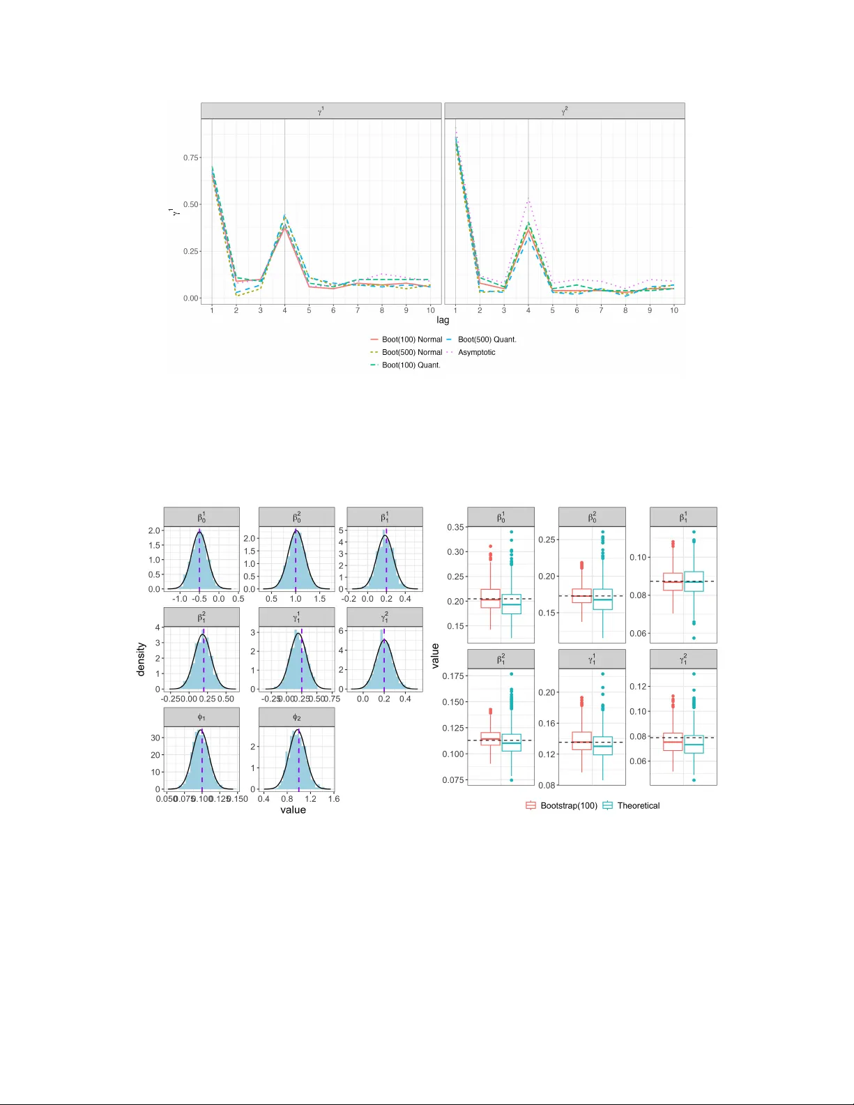
Mixed Time Series Quasi-Lik eliho o d Mo dels for Unco v ering Co vid-19 Viral Load and Mortalit y Dynamics Kejin W u ∗ Dep artment of Mathematics and Statistics, L oyola University Chic ago, USA Raanju R. Sundarara jan † Dep artment of Statistics and Data Scienc e, Southern Metho dist University, USA Mic hel F.C. Haddad ‡ Dep artment of Business A nalytics and Applie d Ec onomics, Que en Mary University of L ondon, UK Luiza S.C. Piancastelli § Scho ol of Mathematics and Statistics, University Col le ge Dublin, R epublic of Ir eland W agner Barreto-Souza ¶ Scho ol of Mathematics and Statistics, University Col le ge Dublin, R epublic of Ir eland Marc h 30, 2026 Abstract Accurate real-time monitoring of disease transmission is crucial for epidemic con trol, which has con ven tionally relied on rep orted cases or hospital admissions. Suc h metrics are frequently sus- ceptible to delays in rep orting, v arious forms of bias, and under-ascertainment. Cycle threshold v alues obtained from rev erse transcription quan titativ e polymerase c hain reaction offer a promis- ing alternative, serving as a pro xy for viral load. In this paper, we aim to join tly model the viral load and the n umber of deaths (mortalit y), whic h in volv es a contin uous b ounded and a count time series, and therefore, a prop er mixed-t yp e mo del is needed. This is the moti- v ation to in tro duce a new mixed-v alued time series quasi-lik eliho o d ( MixTSQL ) model capable of analyzing multiv ariate time series of differen t types, lik e contin uous, discrete, bounded, and con tinuous p ositiv e. The MixTSQL mo del only requires a mean-v ariance specification with no dis- tributional assumptions needed, and allo ws for testing Granger causality . Statistical guaran tees are pro vided to ensure consistency and asymptotic normalit y of the proposed quasi-maxim um lik eliho o d estimators. W e analyze w eekly viral load and Co vid-19 death coun ts in S˜ ao P aulo, Brazil, using our MixTSQL mo del, which not only establishes the temp oral order in whic h viral load Granger-causes mortality but also offers a comprehensiv e joint statistical analysis. Keywor ds: Mixed-v alued time series, Granger causalit y , Quasi maxim um lik eliho o d estimator, Co vid-19. ∗ e-mail : kwu8@luc.edu † e-mail : rsundarara jan@mail.sm u.edu ‡ e-mail : m.haddad@qmul.ac.uk § e-mail : luiza.piancastelli@ucd.ie ¶ e-mail : wagner.barreto-souza@ucd.ie (corresponding author) 1 1 In tro duction Ev ents of epidemics and pandemics represent widespread o ccurrences of infectious diseases that increase death rates across regions. The frequency of such even ts has grown ov er the past hundred y ears, driven b y factors suc h as in tensified global mobilit y , urban expansion, and increased exploita- tion of natural ecosystems. In response, considerable p olicy efforts ha v e emphasized the imp ortance of detecting and containing disease outbreaks with pandemic p oten tial, alongside inv estments to im- pro ve public health preparedness and system resilience ( Madha v et al. , 2017 ). The global Co vid-19 pandemic was precipitated by the Severe Acute Respiratory Syndrome Coronavirus 2 (SARS-CoV- 2). The virus propagates betw een human hosts via respiratory aerosol particles. Considering the n umber of related death coun ts, Brazil is the second most affected coun try in the w orld. During the p eak of the Covid-19 crisis in Brazil, daily mortalit y figures exceeded 4 , 000 fatalities attributable to the disease. Ev en after the most critical momen ts of the global pandemic, many streams of virus ha ve emerged in differen t parts of the world. Recen t examples include the v arian t Nim bus (NB.1.8.1), and a new subv ariant of the Omicron known as Stratus (XFG), among others ( Geddes , 2025 ). The ability to generate reliable epidemiological predictions and causal relationships is highly desirable. The timely implementation of evidence-based policy interv en tions (e.g., so cial distancing proto cols) commonly mitigates mortality rates. There exists a substantial theoretical justifica- tion to p osit that heterogeneity in individual transmission capability may profoundly impact the progression and dynamics of a pandemic episo de ( Lloyd-Smith et al. , 2005 ). Con ven tionally , epi- demiological surveillance relies up on rep orted cases, hospital admissions, or related v ariables (e.g., p ositivit y rate, hospital av erage stay). Ho wev er, such metrics are frequently susceptible to rele- v an t cav eats and limitations. W e assess the utility of viral load estimates derived from reverse transcription quantitativ e p olymerase c hain reaction (R T-qPCR) cycle threshold (Ct) v alues as a promising alternativ e for monitoring epidemic dynamics ( Lim et al. , 2024 ). It also merits ackno wl- edgmen t that viral load constitutes a univ ersally applicable measure of pathogenic progression. Therefore, the presen t w ork is not exclusively pertinent to SARS-CoV-2 infections, b eing equally useful considering future episo des of epidemics or pandemics caused b y a diverse range of viruses. In this pap er, we aim to study and understand the joint dynamics of the Covid-19 viral load, whic h is defined in terms of Ct, and its asso ciated mortality (num b er of deaths). W e consider w eekly data from S˜ ao P aulo, Brazil, with the sampling p erio d spanning from the 20th Marc h 2020 to the 22nd May 2022. This data inv olv es a contin uous b ounded (viral load) and a coun t (mortalit y) time series, and therefore, a prop er mixed-type mo del is needed. This is the motiv ation to in tro duce a new mixed-v alued time series quasi-likelihoo d mo del (in short MixTSQL ) capable of analyzing m ultiv ariate time series of different t yp es, like contin uous, discrete, b ounded, and con tinuous p ositiv e-v alued, and whic h only requires a mean-v ariance sp ecification instead of a full distributional assumption. The study of interactions among time series has b een of interest in areas such as finance, economics, and neuroscience since the seminal pap er b y Granger ( 1969 ), where the concept of Granger causalit y was introduced. The ma jority of the approac hes for testing Granger causalit y relies on the linear vector autoregressive (V AR) mo del, which relies on the multiv ariate normal distribution. On the other hand, time series data may b e of a differen t nature suc h as counts, p ositiv e contin uous, or b ounded v alued. The causality problem inv olving just count time series has b een addressed b y Chen and Lee ( 2017 ), Lee and Lee ( 2019 ), and Piancastelli et al. ( 2023 ), while T ank et al. ( 2021 ) prop osed a test for dealing with categorical time series. F or a review that 2 accoun ts for the most imp ortan t developmen ts and recent adv ances in Granger causalit y , w e refer to the w ork b y Sho jaie and F o x ( 2022 ). One of the few pap ers handling mixed-v alued time series is due to Piancastelli et al. ( 2024 ), where a class of mixed-v alued time series generalized linear mo dels (GLMs) was prop osed. One of the requiremen ts of these models is that the conditional distributions (giv en past observ ations) m ust b elong to the exp onen tial family , and therefore cannot b e used to analyze our data since one of the comp onen ts (viral load) is b ounded. In fact, our formulation can b e seen as a generalization of the models prop osed b y Piancastelli et al. ( 2024 ) in the same sense quasi-lik eliho o d mo dels extend GLMs. W e highligh t that an important and rather distinctive adv an tage of the mo dels introduced in the present w ork is that only a mean-v ariance sp ecification needs to b e sp ecified. No sp ecific distri- butional assumptions are needed, whic h implies more flexibility when compared to fully parametric mo dels. Under the assumption that the mean function’s structural sp ecification is correct, we pro- vide theoretically consisten t estimation for the mo del coefficients. Another highly relev ant feature is that w e are able to test Granger causality b et ween t wo time series that can b e binary , coun ts, con tinuous, p ositiv e, and b ounded-v alued. W e summarize the main con tributions of this paper in what follo ws. • The presen t w ork focuses on the use of in trinsic information contained within the cycle thresh- old v alues (Ct) derived from the R T-qPCR assays, through viral load, which is defined as one min us the standardized Ct, and the study of its relationship with mortality counts. With this c hallenge in mind, a new quasi-lik eliho od mo del, termed as MixTSQL , is introduced and designed for analyzing the mixed-v alued time series Co vid-19 data. Instead of assuming a fully parametric m ultiv ariate time series mo del, MixTSQL mo dels only imp ose assumptions on the first tw o cumulan ts of the time series. Then, a quasi-likelihoo d approach is developed for estimation and inference purp oses. As long as the structural assumption on the mean function is correct, consistency in mean estimation is obtained. Statistical guarantees to en- sure consistency and asymptotic normality of the prop osed quasi-likelihoo d estimators are pro vided. • V ery few w orks consider testing Granger causalit y in mean and v ariance simultaneously . In the presen t w ork, w e provide the necessary and sufficient conditions to chec k the Granger causalit y in mean and v ariance sim ultaneously . This test is critically imp ortant while understanding the lead-lag effect of viral load on subsequen t mortalities. The individual definitions of Granger causalit y with resp ect to the mean or with resp ect to the v ariance can b e found in ( Granger , 1969 ) and Granger et al. ( 1986 ), resp ectiv ely; see also Sto c k and W atson ( 1989 ); Lee ( 1992 ); M ˚ ansson and Sh ukur ( 2009 ); C ¸ evik et al. ( 2018 ) for a list of wide-ranging applications. • Extensiv e sim ulation experiments are conducted to study the performance of the new quasi- lik eliho o d estimation tec hnique. The simulation settings are carefully designed to closely mimic the Co vid-19 data v ariables under consideration. It is w ell kno wn that standard error computations based on theory-driven analytical expressions need not b e accurate in finite sample situations; see Barreto-Souza et al. ( 2025 ) for a recen t work comparing theoretical and b o otstrap approac hes in the context of count time series mo dels. Our sim ulation studies, ho wev er, rev eal that b oth theoretical and b o otstrap approaches work well in finite sample settings. W e also discuss connections b etw een the asymptotic results on the estimators and the empirical results from this simulation study . 3 • W e in v estigate the impact of viral load on the mo deling and forecasting of mortalit y , while also testing for Granger causalit y . This nov el approach offers v aluable insights for future outbreaks of viral epidemics or pandemics. W e p erform an out-of-sample forecasting exercise, whic h shows that the MixTSQL mo del yields a lo wer ro ot mean forecasting error compared to a standard Gaussian linear mo del. Moreov er, our mo del provides strong evidence of Granger causalit y from viral load to mortalit y coun ts. The pap er unfolds as follows. In Section 2 , we describ e the Covid-19 data from Brazil in detail. In Section 3 , we in tro duce our class of MixTSQL models for analyzing mixed-v alued time series data. This section also includes mo del inference based on the quasi-likelihoo d approac h, statistical guaran tees to ensure consistency and asymptotic normality of the prop osed estimators, and a Granger causalit y test. Simulation exp erimen ts and p erformance assessment results are reported in Section 4 . A full statistical data analysis of the Covid-19 viral load and mortalit y is provided in Section 5 . Section 6 con tains our concluding remarks, including possible future research. This pap er contains Supplemen tary Material with all technical pro ofs of theorems and propositions. 2 Co vid-19 data description Although daily rep orted p ositiv e cases constitute the primary surveillance measure for Covid-19 incidence, these data are ackno wledged to exhibit relev an t cav eats and limitations - e.g., rep ort- ing delays, selection bias, under-ascertainmen t of actual infection rates ( Flaxman et al. , 2020 ). Moreo ver, its quan tification of infectivity is restricted to a dichotomous assessmen t of an individ- ual’s con tagiousness level. This binary characterization constitutes a significant metho dological constrain t in conducting meaningful and timely prognostic analyses. Ct v alues consist of a contin uous v ariable that is a pro xy of viral load, indicating the amount of viral genetic material that is presen t in a patien t sample. Despite its p oten tial adoption for monitor- ing and mitigation purp oses in cases of epidemics and pandemics, Ct v alues are mostly not publicly accessible. A low Ct v alue reflects a high concentration of viral genetic material, which is typically asso ciated with a higher risk of infectivity . Conv ersely , a high Ct v alue reflects a lo w concentra- tion of viral genetic material, which is t ypically associated with a low er risk of infectivity ( Public Health England , 2020 ). Not withstanding in ter-individual v ariability , sp ecimen heterogeneit y , and platform-dep enden t differences in assa y p erformance, Ct v alues offer a probabilistic indicator of the time elapsed since infection acquisition. Accumulating evidence suggests a temp oral asso ciation b et w een epidemic tra jectory and the mean Ct v alues observed in SARS-CoV-2–positive sp ecimens ( Kutta et al. , 2025 ; Ha y et al. , 2021 ). An expanding epidemic or pandemic, characterized by a predominance of recent infections, exhibits higher viral loads and lo wer mean Ct v alues at the p opulation lev el. Conv ersely , a declining epidemic or pandemic, in which a greater prop ortion of infections are in later stages, demonstrates lo wer viral loads and corresp ondingly elev ated mean Ct v alues. Moreo ver, previous studies hav e rep orted a p ositiv e association betw een viral load and patients at higher risk of se v ere outcomes, including death - e.g., Magleby et al. ( 2021 ), F a ´ ıco-Filho et al. ( 2020 ). Dra wing on this insight, we in tro duce the metho dological framew ork detailed in the subsequent section. It is worth mentioning that w orks inv olving viral load data are still scarce due to the c hallenges in collecting suc h datasets. Th us, more studies are needed to confirm this p ositiv e asso ciation - preferably , exploring larger sample sizes suc h as the one used in the presen t study . 4 The dataset explored in this work comprises raw PCR test results, including Ct v alues for SARS-CoV-2, obtained from a leading clinical diagnostic lab oratory in Brazil (DB Diagn´ osticos). This dataset is complemented with a public related v ariable, namely the daily coun t of deaths attributed to the Co vid-19. The dataset con tains 342,699 individual PCR testing records. The sampling p eriod spans from the 20th March 2020 to the 22nd May 2022. While sp ecimens w ere collected across around 2,100 testing sites nationwide, all analyses were conducted at a cen tralized lab oratory facility lo cated in S˜ ao P aulo. The Ct time series is b ounded and w e standardized it to the unit in terv al (0 , 1). Then, the viral load time series is defined as viral load = 1 − standardized( C t ). The viral load and mortalit y biv ariate mixed-v alued time series, observed at the daily frequency in S˜ ao Paulo, Brazil, is presen ted in Figure 1 . The data at the daily frequency show a n umber of zero or close to zero deaths and high v olatility , which brings difficulties to mo deling. Not only do es this b eha vior cause numerical instabilit y , but also do es not reflect reality . Zero daily deaths are most often due to a delay in reporting, occurring especially on week ends. Figure 1: Daily observ ations of viral load and death counts in S˜ ao P aulo, Brazil, from 2020-03-26 to 2022-05-22. Therefore, we aggregate and analyze the t w o time series at a weekly frequency . Compared to the daily frequency data, the weekly data is preferable considering that commonly there are more PCR tests p erformed at the b eginning of each week as a consequence of the fact that p eople get together more often during w eekends. As a result of weekly aggregation, the n umber of zero deaths decreases significantly and, consequen tly , the asso ciated volatilit y , as illustrated in Figure 2 . In the presen t w ork, the analyses are p erformed at the weekly frequency of the data. Each transformed tra jectory comprises of n = 112 observ ations. It must also b e noted that almost all existing studies exploring pandemic dynamics using Ct v alues work with a substantially smaller sample size compared to the present work; see Ha y et al. ( 2021 ), Y agci et al. ( 2020 ) for examples. The primary ob jective of this pap er is to jointly mo del viral load and mortalit y in order to b etter understand their dynamic relationship and inv estigate prop erties such as Granger causalit y . Giv en the mixed-t yp e nature of the time series data and the lac k of proper models existing in the literature to handle this problem, a nov el metho dological approach is required, which is in tro duced in the follo wing section. 5 Figure 2: W eekly observ ations of viral load and death counts in S˜ ao Paulo, Brazil, from 2020-03-26 to 2022-05-22. 3 Mixed Time Series Quasi-Lik eliho o d Mo dels In this section, we present a nov el metho dology for analyzing Co vid-19 viral load dynamics and its asso ciation with related mortality . Our approac h is grounded in a quasi-lik eliho od framew ork and extends the mixed time series generalized linear mo dels introduced by Piancastelli et al. ( 2024 ), whic h are based on exp onen tial family form ulations. This extension is essen tial for our applica- tion, as it accommo dates key features of the Co vid-19 time series data considered in this study , particularly the join t modeling of b ounded and coun t-v alued biv ariate time series. 3.1 Mo del sp ecification W e b egin by introducing an important ingredient of our mo dels. W e consider the class of quasi- lik eliho o d (QL) mo dels prop osed b y W edderburn ( 1974 ), which is defined by specifying the first t wo cum ulants of a random v ariable (sa y Y ), the mean µ and the v ariance V ar( Y ) = ϕV ( µ ), plus a log-quasi-likelihoo d function assuming the form Q ( y ; µ ) = 1 ϕ Z µ y y − ω V ( ω ) dω , (1) where ϕ > 0 is a disp ersion parameter. The following notation is considered in this case, which implicitly dep ends on the v ariance function: Y ∼ QL( µ, ϕ ). A notable adv antage of the QL mo deling approach is that there are more possibilities to sp ecify the v ariance function than in the exp onen tial family . This allo ws, for example, to handle contin uous b ounded-v alued data. The QL mo dels con tain the exp onen tial family (GLM when considering cov ariates) as a sp ecial case, dep ending on the v ariance function sp ecification. Let { Y 1 t } t ∈ N and { Y 2 t } t ∈ N b e tw o time series and denote the sigma-algebras F (1) t − 1 = σ ( Y 1 t − 1 , Y 1 t − 2 , . . . ), F (2) t − 1 = σ ( Y 2 t − 1 , Y 2 t − 2 , . . . ) and F (1 , 2) t − 1 = σ ( F (1) t − 1 , F (2) t − 1 ). W e now define our class of biv ariate mixed time series mo dels as follo ws. Definition 3.1. [ MixTSQL mo del] The mixe d-value d time series quasi-likeliho o d mo del ( MixTSQL ) is define d by the time series ve ctor { ( Y 1 t , Y 2 t ) } t ∈ N , with Y 1 t and Y 2 t c onditional ly indep endent given 6 F (1 , 2) t − 1 for al l t , and satisfying Y 1 t |F (1 , 2) t − 1 ∼ QL (1) ( µ 1 t , ϕ 1 ) and Y 2 t |F (1 , 2) t − 1 ∼ QL (2) ( µ 2 t , ϕ 2 ) , with ν 2 t ≡ g 2 ( µ 2 t ) ≡ β (2) 0 + p X i =1 β (2) i e Y 2 t − i + k X l =1 γ (2) l e Y 1 t − l , (2) ν 1 t ≡ g 1 ( µ 1 t ) ≡ β (1) 0 + r X i =1 β (1) i e Y 1 t − i + s X l =1 γ (1) l e Y 2 t − l , (3) wher e g 1 ( · ) and g 2 ( · ) ar e link functions assume d to b e c ontinuous, invertible, and twic e differ entiable, with e Y 1 t = T 1 ( Y 1 t ) and e Y 2 t = T 2 ( Y 2 t ) b eing ade quate tr ansformations of the original time series, β (1) 0 , . . . , β (1) r , β (2) 0 , . . . , β (2) p , γ (1) 1 , . . . , γ (1) s , and γ (2) 1 , . . . , γ (2) k ar e r e al-value d p ar ameters, and ϕ 1 and ϕ 2 ar e disp ersion p ar ameters. Remark 3.2. The tr ansforme d time series e Y 1 t and e Y 2 t in ( 2 ) and ( 3 ), r esp e ctively, via T 1 ( · ) and T 2 ( · ) ar e ne c essary sinc e we ar e mo deling the tr ansforme d me an-r elate d p ar ameters. In gener al, we wil l c onsider T 1 ( y ) = g 1 ( y ) and T 2 ( y ) = g 2 ( y ) unless some slight mo dific ation is ne c essary such as in the c ount time series c ase. Mor e sp e cific al ly, if Y 2 t is a time series of c ounts and g 2 ( y ) = log y , we take T 2 ( y ) = log( y + 1) b e c ause the lo g-function is not b e wel l-define d at y = 0 . This tr ansformation te chnique is inspir e d by the lo g-line ar INGARCH mo dels by F okianos and Tjøstheim ( 2011 ). The choic es for the tr ansforme d time series b eing the link functions or slight mo dific ations of them wil l ke ep ν 1 t and ν 2 t in the same sc ales of e Y 1 t and e Y 2 t , r esp e ctively. The sup erscripts (1) and (2) in QL (1) and QL (2) imply that differ ent QL mo dels c an b e use d for Y 1 t and Y 2 t . One of our aims is to test if { Y 1 t } t ∈ N causes to { Y 2 t } t ∈ N in mean ( Granger , 1969 ), that is Pr  E ( Y 2 t |F (2) t − 1 )  = E ( Y 2 t |F (1 , 2) t − 1 )  > 0 . (4) Throughout this pap er, w e consider the Granger causality test for whether { Y 1 ,t } t ∈ N Granger-causes { Y 2 ,t } t ∈ N . The test for the rev erse direction pro ceeds analogously . The choice for the v ariance function will dictate how the v ariance will dep end on the mean. As a further consequence, the series { Y 1 t } t ∈ N can ha ve a causal effect on the series { Y 2 t } t ∈ N in b oth the mean and v ariance sim ultaneously . According Granger et al. ( 1986 ), { Y 1 t } t ∈ N causes to { Y 2 t } t ∈ N in v ariance if Pr  V ar( Y 2 t |F (2) t − 1 )  = V ar( Y 2 t |F (1 , 2) t − 1 )  > 0 . (5) More sp ecifically , the inequality in ( 5 ) is Pr E "  Y 2 t − E ( Y 2 t |F (1 , 2) t − 1 )  2      F (2) t − 1 #  = E "  Y 2 t − E ( Y 2 t |F (1 , 2) t − 1 )  2      F (1 , 2) t − 1 #! > 0 . (6) Readers can refer to Guo et al. ( 2014 ) for simultaneous causalit y testing in the factor double autoregressions problem. F ollo wing their approac h, w e consider the follo wing. Pr E "  Y 2 t − E ( Y 2 t |F (2) t − 1 )  2      F (2) t − 1 #  = E "  Y 2 t − E ( Y 2 t |F (1 , 2) t − 1 )  2      F (1 , 2) t − 1 #! > 0 . (7) W e no w pro vide a proposition that sho ws that v erifying inequalit y ( 7 ) is sufficien t to test for Granger causality in mean and v ariance sim ultaneously . 7 Prop osition 3.3. Ine quality ( 7 ) holds if at le ast one of the ine qualities in ( 4 ) and ( 5 ) holds. In practice, it is common to assume a data-generating mo del to capture the underlying dynamics of observ ed time series, such as ARMA mo dels for univ ariate data or V AR mo dels for multiv ariate settings. Subsequently , the Granger causality test can b e p erformed b y inferring on the v alues of certain mo del co efficien ts. How ever, these classical mo dels often imp ose to o many restrictions such as normalit y and con tinuous-v alued time series, b esides b eing susceptible to mo del misspecification. The prop osed class of MixTSQL mo dels is robust to mo del missp ecification due to its quasi-lik eliho o d approac h and offers a flexible framew ork for testing Granger causalit y among time series of differen t t yp es, including con tinuous, p ositiv e, coun t, bounded, and binary v ariables. Under the proposed MixTSQL mo del defined in Definition 3.1 , testing for Granger c ausalit y of the time series Y 1 ,t on Y 2 ,t in b oth mean and v ariance is equiv alent to testing whether the Granger causalit y parameters γ (2) l are nonzero for l = 1 , . . . , k , as established in Prop osition 3.5 . W e no w in tro duce a tec hnical assumption required to prov e suc h a result. A Granger causality test will b e discussed in Subsection 3.3 . • A1. The σ -algebras σ ( σ ( Y 2 t ) , F (2) t − 1 ) and F (1) t − 1 are indep enden t when γ (2) l = 0 ∀ l ∈ { 1 , 2 , . . . , k } . Remark 3.4. Assumption A1 implies that the r andom variable Y 2 t and the se quenc e { Y 1 t − 1 , Y 1 t − 2 , . . . } ar e c onditional ly indep endent given F (2) t − 1 when γ (2) l = 0 ∀ l ∈ { 1 , 2 , . . . , k } . Prop osition 3.5. Under Assumption A1, the ine quality in ( 7 ) holds if and only if γ (2) l  = 0 for some l ∈ { 1 , 2 , . . . , k } . Assume that { ( y 1 t , y 2 t ) } n t =1 is a realization of a mixed-v alued time series from the MixTSQL mo del describ ed in Definition 3.1 . Define the parameter vector θ = ( θ (1) , θ (2) ) ⊤ . Note that ϕ 1 and ϕ 2 are the n uisance parameters. The quasi log-likelihoo d function, sa y e Q ( θ ), is giv en by e Q ( θ ) = n X t = m +1 { Q 1 ( y 1 t ; µ 1 t ) + Q 2 ( y 2 t ; µ 2 t ) } , (8) where m = max( p, q , r , s ), Q j ( · ; · ) assumes the form from ( 1 ) with series specific function V ( · ) := V j ( · ), for j = 1 , 2. The quasi-maxim um likelihoo d estimator (QMLE) of θ (conditional on { ( y 1 i , y 2 i ) } m i =1 ) is given b y b θ := arg min θ − e Q ( θ ). The quasi score function associated with e Q ( θ ) is U ( θ ) ≡ ∂ e Q ( θ ) ∂ θ = n X t = m +1 U t ( θ ), where U t ( θ ) =  1 ϕ 1 y 1 t − µ 1 t V ( µ 1 t ) 1 g ′ 1 ( µ 1 t ) ∂ ν 1 t ∂ θ (1) , 1 ϕ 2 y 2 t − µ 2 t V ( µ 2 t ) 1 g ′ 2 ( µ 2 t ) ∂ ν 2 t ∂ θ (2)  ⊤ , (9) ∂ ν 1 t ∂ θ (1) = (1 , e Y 1 t − 1 , . . . , e Y 1 t − r , e Y 2 t − 1 , . . . , e Y 2 t − s ) ⊤ , ∂ ν 2 t ∂ θ (2) = (1 , e Y 2 t − 1 , . . . , e Y 2 t − p , e Y 1 t − 1 , . . . , e Y 1 t − k ) ⊤ , (10) 8 with θ (1) = ( β (1) 0 , β (1) 1 , . . . , β (1) r , γ (1) 1 , . . . , γ (1) s ) ⊤ and θ (2) = ( β (2) 0 , β (2) 1 , . . . , β (2) p , γ (2) 1 , . . . , γ (2) k ) ⊤ . If the disp ersion parameters are unknown, they can b e estimated via metho d of moments. Sp ecifically , these estimators assume the forms b ϕ 1 = n X t = m +1 ( Y 1 t − b µ 1 t ) 2 n X t = m +1 V 1 ( b µ 1 t ) and b ϕ 2 = n X t = m +1 ( Y 2 t − b µ 2 t ) 2 n X t = m +1 V 2 ( b µ 2 t ) , (11) where b µ 1 t and b µ 2 t are the quasi-likelihoo d estimators of µ 1 t and µ 2 t , resp ectiv ely . In the following subsection, we pro vide statistical guarantees to ensure consistency and asymptotic normality of the quasi-lik eliho o d estimators. 3.2 Statistical guarantees and asymptotics W e first consider the consistency of the quasi-maximum lik eliho o d estimator (QMLE) b θ . T o sim- plify the notation, w e denote Q 1 ( Y 1 t ; µ 1 t ) and Q 2 ( Y 2 t ; µ 2 t ) from ( 8 ) by Q 1 t ( θ (1) ) and Q 2 t ( θ (2) ), resp ectiv ely , where the parameter v ector θ = ( θ (1) , θ (2) ) ⊤ , with θ (1) and θ (2) as defined ab o v e. This enables writing e Q ( θ ) = P n t = m +1 { Q 1 t ( θ (1) ) + Q 2 t ( θ (2) ) } . Note that, from the MixTSQL mo del’s Def- inition 3.1 , ν 1 t and ν 2 t dep end exclusively on θ (1) and θ (2) , respectively . This allows us to write these tw o quantities as ν 1 t ( θ (1) ) and ν 2 t ( θ (2) ). Next, a few tec hnical assumptions are provided and these are needed to establish consistency of the proposed estimators. • A2. The series { Y t = ( Y 1 t , Y 2 t ) } is stationary and ergodic. • B1. The true v alue θ 0 := ( θ (1) 0 , θ (2) 0 ) ⊤ is an interior p oin t in Θ := Θ 1 × Θ 2 whic h is a compact set in R r + s +1 × R p + k +1 . • B2. ν 1 t ( θ (1) 0 ) = ν 1 t ( θ (1) ) and ν 2 t ( θ (2) 0 ) = ν 2 t ( θ (2) ) if and only if θ (1) 0 = θ (1) and θ (2) 0 = θ (2) , resp ectiv ely . • C1. E  sup θ ∈ Θ   Q 1 t ( θ (1) ) + Q 2 t ( θ (2) )    < ∞ . • C2. E  − Q 1 t ( θ (1) ) − Q 2 t ( θ (2) )  has a unique minimum at θ 0 . Remark 3.6. It is imp ortant to note that The or em 3.7 c ould stil l hold even without the stationarity c ondition fr om Assumption A2. F or example, we c an assume 1 n − m P n t = m +1 [inf θ ∈ B η 0 ( θ ∗ ) − Q t ( θ ) − E  inf θ ∈ B η 0 ( θ ∗ ) − Q t ( θ )  ] → 0 for ∀ θ ∗ , which is similar to Kolmo gor ov’s str ong law of lar ge numb ers, wher e B η ( θ ∗ ) = { θ ∈ Θ : ∥ θ − θ ∗ ∥ < η } b e an op en neighb orho o d of θ ∗ and − Q t ( θ ) := − Q 1 t  θ (1)  − Q 2 t  θ (2)  . F urther, we would also ne e d 1 n − m P n t = m +1 E ( − Q t ( θ )) to have a unique minimum at θ 0 and that 1 n − m P n t = m +1 E ( − sup θ ∈ Θ Q t ( θ )) is finite. T o simplify te chnic al exp osi- tion, we assume A2 thr oughout this p ap er. Assumption B2 ensur es mo del identifiability. Combining subse quent assumption B3, Pr op osition 3.8 wil l show assumptions B1 to B3 imply C1 to C2 for sp e- cific quasi-likeliho o d mo dels. Assumptions C1 to C2 ar e ne e de d to establish c onsistency as il lustr ate d in The or em 3.7 . Theorem 3.7. Under Assumptions A2, B1, C1-C2, b θ p → θ 0 , as n → ∞ . 9 The pro of of Theorem 3.7 follows closely to the pro of of Theorem 2.1 of Zh u and Ling ( 2011 ) with the metho ds inspired by Huber et al. ( 1967 ). Note that the ab ov e consistency result can b e established for any pair of quasi-likelihoo d functions Q 1 t ( θ (1) ) and Q 2 t ( θ (2) ) as long as they s atisfy assumptions C1-C2. The key assumption for obtaining consistency is that the mean functions µ 1 t and µ 2 t are mo deled correctly . Motiv ated by the real data application considered in this pap er in Section 5 , we build Q 1 t ( θ (1) ) and Q 2 t ( θ (2) ) based on the v ariance function sp ecifications V 1 ( µ 1 ) = µ 1 (1 − µ 1 ) and V 2 ( µ 2 ) = µ 2 , resp ectiv ely , which mimic the mean-v ariance relationship of the (for example) b eta (parameterized in terms of mean and disp ersion parameters) and double Poisson ( Efron , 1986 ) distributions, which are used in practice for modeling counts and con tinuous b ounded-v alued data. Next, w e provide v erification of assumptions C1-C2 based on sp ecific choices of Q 1 t ( θ (1) ) and Q 2 t ( θ (2) ). In other w ords, with the discrete series Y 2 t b eing mo deled via double P oisson distribution and Y 1 t via Beta distribution, w e ha ve in the v ariance functions V 1 ( µ ) = µ (1 − µ ) and V 2 ( µ ) = µ . After omitting a few constant terms, w e write Q 1 ( y 1 t ; µ 1 t ) ∝ y 1 t log( µ 1 t ) + (1 − y 1 t ) log (1 − µ 1 t ) , Q 2 ( y 2 t ; µ 2 t ) ∝ y 2 t log( µ 2 t ) − µ 2 t . (12) Note that in order to ease notation usage, the dependency of µ 1 t and µ 2 t on θ (1) and θ (2) is suppressed. W e also consider the link functions g 1 ( x ) = log( x 1 − x ) and g 2 ( x ) = log( x ). Next, w e state an additional assumption required to establish the consistency of the estimators under the mo del sp ecification given ab o ve. • B3. Assume that E ( Y 2 2 t ) < ∞ , max i =1 ,...,p E ( | Y 2 t Y 2 t − i | ) < ∞ , max i =1 ,...,p E   Y 2 2 t − i p Y j =1 ( Y 2 2 t − j + 1)   < ∞ , max i =1 ,...,s E   Y 2 2 t − i s Y j =1 ( Y 2 2 t − j + 1)   < ∞ , max i =1 ,...,p E   Y 2 2 t Y 2 2 t − i p Y j =1 ( Y 2 2 t − j + 1)   < ∞ . Next, we state a prop osition that shows that the consistency result in Theorem 3.7 holds for our case under Assumptions B1-B3. Prop osition 3.8. Supp ose that Assumptions B1-B3 hold. Then, for the functions Q 1 t ( θ (1) ) and Q 2 t ( θ (2) ) describ e d in ( 12 ), Assumptions C1-C2 ar e satisfie d. T o e stablish the large sample distribution of the QMLE b θ , we need a final additional tec hnical assumption as follo ws. • B4. The matrices E  ∂ ν 1 t ∂ θ (1) ∂ ν ⊤ 1 t ∂ θ (1)  and E  ∂ ν 2 t ∂ θ (2) ∂ ν ⊤ 2 t ∂ θ (2)  are b oth positive definite. Theorem 3.9. Under assumptions B1-B4, we have √ n ( b θ − θ 0 ) d → N ( 0 , Σ ) , as n → ∞ , (13) 10 wher e Σ = Ω − 1 2 Ω 1 Ω − 1 2 , Ω 1 ≡ lim n →∞ E n − 1 ∂ e Q ( θ ) ∂ θ ∂ e Q ( θ ) ∂ θ ⊤     θ = θ 0 ! ; Ω 2 ≡ lim n →∞ E n − 1 ∂ 2 e Q ( θ ) ∂ θ ∂ θ ′     θ = θ 0 ! , with the limits denoting limits in pr ob ability. Remark 3.10. The pr o of of The or em 3.9 is inspir e d by the pr o of te chnique utilize d in The or em 4.1.3 of Amemiya ( 1985 ). In pr actic e, Σ c an b e c onsistently estimate d by b Σ = S − 1 2 ( b θ ) S 1 ( b θ ) S − 1 2 ( b θ ) , wher e S 1 ( θ ) = n − 1 n X t = m +1 U t ( θ ) U t ( θ ) ⊤ and S 2 ( θ ) = n − 1 n X t = m +1 H t ( θ ) , with U t ( θ ) given by ( 9 ), and H t ( θ ) ≡ E  − ∂ U t ( θ ) /∂ θ   F (1 , 2) t − 1  =     1 ϕ 1 V ( µ 1 t )( g ′ 1 ( µ 1 t )) 2 ∂ ν 1 t ∂ θ (1) ∂ ν ⊤ 1 t ∂ θ (1) 0 0 1 ϕ 2 V ( µ 2 t )( g ′ 2 ( µ 2 t )) 2 ∂ ν 2 t ∂ θ (2) ∂ ν ⊤ 2 t ∂ θ (2)     , with ϕ 1 and ϕ 2 r eplac e d by c onsistent estimators if unknown. Ther efor e, the standar d err ors of b θ c an b e assesse d via the matrix n − 1 b Σ . T o show that S 2 ( b θ ) p → Ω 2 , (14) the ide a is to first ar gue that S 2 ( θ ) = n − 1 n X t = m +1 H t ( θ ) p → Ω 2 uniformly in a neighb orho o d of θ 0 . Then, ( 14 ) holds for any se quenc e of estimators wher ein b θ p → θ 0 . In other wor ds, it is p ossible for us to c onsider H t ( θ ) in a “c onditional exp e cte d version” of the hessian matrix (inste ad of just the hessian matrix) sinc e we c an estimate Ω 2 wel l by applying the tower pr op erty. As a r esult, the c omputation of the estimator for Ω 2 is simplifie d sinc e the c omputation of al l terms of the hessian matrix is cumb ersome. 3.3 Granger causality test The in terest here is in testing if the time series { Y 1 t } t ∈ N Granger causes { Y 2 t } t ∈ N . This, in terms of comp eting hypotheses, can b e formulated as H 0 : γ (2) l = 0 for all l ∈ { 1 , . . . , k } , v ersus H 1 : γ (2) l  = 0 for some l ∈ { 1 , . . . , k } . The null h yp othesis H 0 implies no Granger causalit y while the alternativ e h yp othesis indicates Granger causality . W e will use a lik eliho od ratio test based on quasi-lik eliho o d to perform suc h a h yp otheses testing. T o do this, we define the vector of the biv ariate time series and its asso ciated conditional biv ariate mean v ector b y y and µ , resp ectiv ely , and the deviance function D ( y ; µ ) as t wo times the difference of the rescaled quasi-likelihoo d functions under the saturated ( y = µ ) and unsatured mo dels: D ( y ; µ ) = 2 ( n X t = m +1 [ ϕ 1 Q 1 ( y 1 t ; y 1 t ) + ϕ 2 Q 2 ( y 2 t ; y 2 t )] − n X t = m +1 [ ϕ 1 Q 1 ( y 1 t ; µ 1 t ) + ϕ 2 Q 2 ( y 2 t ; µ 2 t )] ) = − 2 n X t = m +1 [ ϕ 1 Q 1 ( y 1 t ; µ 1 t ) + ϕ 2 Q 2 ( y 2 t ; µ 2 t )] . 11 Denote by b µ and b µ 0 the quasi-likelihoo d estimates of the biv ariate conditional mean vector under the unrestricted and restricted (n ull hypothesis) mo dels. Then, the difference of the deviance under the restricted and unrestricted models is D ( y ; b µ 0 ) − D ( y ; b µ ) = ϕ 2 n X t = m +1  Q 2 ( y 2 t ; b µ 2 t ) − Q 2 ( y 2 t ; b µ 0 2 t )  . (15) Under the conditions of Theorem 3.9 , the rescaled (b y ϕ 2 ) quantit y in ( 15 ), denoted b y quasi lik eliho o d ratio (QLR) statistic, satisfies the follo wing con vergence in distribution: QLR = n X t = m +1  Q 2 ( y 2 t ; b µ 2 t ) − Q 2 ( y 2 t ; b µ 0 2 t )  = 1 ϕ 2 n X t = m +1 " Z b µ 2 t y 2 t y 2 t − ω V 2 ( ω ) dω − Z b µ 0 2 t y 2 t y 2 t − ω V 2 ( ω ) dω # d − → χ 2 k , (16) as n → ∞ , where χ 2 k denotes a chi-squared distribution with k degrees of freedom, with ϕ 2 replaced b y a consistent estimator if unkno wn. Note that we are not at the b oundary of the parameter space under H 0 and therefore the asymptotic distribution of the QLR is indeed c hi-squared. The con vergence of the QLR statistic in ( 16 ) will be used in Section 5 to assess the Granger causalit y order in which the Covid-19 viral load influences mortalit y . In this case, the statistic assumes the closed-form QLR = 2 ϕ − 1 2 n X t = m +1  y 2 t log  b µ 0 2 t b µ 2 t 1 − b µ 2 t 1 − b µ 0 2 t  + log  1 − b µ 0 2 t 1 − b µ 2 t  , under the v ariance function choice V 2 ( µ 2 ) = µ 2 (1 − µ 2 ). 4 Sim ulated Exp erimen ts This section assesses the estimation of the MixTSQL mo del parameters and their standard errors via Mon te Carlo sim ulation. F or the latter, w e compare tw o approaches: one based on the asymptotic distribution of the QL estimators (Subsection 3.2 ), and an alternative pseudo-parametric b o ot- strap metho d, which inv olves: (i) fitting the mo del to the observed data; (ii) generating replicated tra jectories using (i) and any distributional assumption that matches the t wo first moments QL sp ecification; (iii) re-estimating parameters via quasi-lik eliho od for each replication; and (iv) com- puting standard errors as the standard deviation of the resulting estimates ov er B replications. This pseudo-parametric b o otstrap approach has b een employ ed by Maia et al. ( 2021 ), where a class of univ ariate semiparametric time series mo dels w as prop osed based on quasi-lik eliho od and laten t factor mo dels. A comparison betw een the theoretical and b o otstrap approaches has b een done previously in the context of count time series mo dels in Barreto-Souza et al. ( 2025 ). In the latter, the authors observ ed that standard errors are underestimated by the asymptotic metho d, and that the b o otstrap is preferable under small samples. It is therefore essential to assess this b ehavior for the MixTSQL mo dels, particularly giv en that our application inv olv es a sample size of n = 112 observ ations. This study is carried out under four settings that v ary in parameter v alues and distributional assumptions to generate time series tra jectories. In Configurations 1 and 2 (C1, C2), the data is sim ulated from a biv ariate b eta-Poisson model (with conditional mean sp ecifications ( 2 ) and ( 3 )) under the parameter v alues specified below and sample size n = 100. 12 • Configuration 1: (b eta-P oisson) β (1) = (1 , 0 . 2) ⊤ , β (2) = (1 , 0 . 2) ⊤ , γ (1) = − 0 . 2, γ (2) = − 0 . 2 , ϕ 1 = 0 . 2, ϕ 2 = 1. • Configuration 2: (b eta-P oisson) β (1) = (1 . 5 , 0 . 2) ⊤ , β (2) = (1 , 0 . 2) ⊤ , γ (1) = ( − 0 . 5 , 0 , 0 , 0 . 3) ⊤ , γ (2) = ( − 0 . 2 , 0 , 0 , 0 . 1) ⊤ , ϕ 1 = 0 . 1, ϕ 2 = 1. Analysis of the cross-correlation function (CCF) of the sim ulated data sho ws that these v alues of γ (1) and γ (2) render cross-correlation cor( Y 1 ,t , Y 2 ,t − 1 ) and cor( Y 1 ,t − 1 , Y 2 ,t ) of ab out − 0 . 30 and − 0 . 17, resp ectiv ely . Fitting b ootstrap SEs for C1 and C2 is carried out under correct mo del sp ecification, i.e., b oth sim ulated data and the bo otstrap replications are generated from the beta-Poisson mo del. This is c hanged in Configuration C3, where the data generation pro cess and b ootstrap distribution are no longer the same. In C3, the tra jectories are sim ulated from a Bessel-P oisson mo del (Bessel distribution is an alternativ e to the b eta mo del, and when parameterized in terms of the mean, matches the v ariance sp ecification ϕ 2 µ 2 (1 − µ 2 ); for instance, see Barreto-Souza et al. ( 2021 )), and the pseudo-parametric b ootstrap replications are gathered from a b eta-Double P oisson specification. This analysis is im- p ortan t for ev aluating the robustness and reliabilit y of the pseudo-parametric bo otstrap standard errors under mo del missp ecification. Notably , the b eta-Double Poisson sp ecification used in the b ootstrap replications offers the most flexible v ariance specification, as it includes nuisance pa- rameters in both directions ( ϕ 1 and ϕ 2 ). This added flexibilit y allows the model to accommo date differen t levels of disp ersion, and we therefore exp ect it to p erform w ell even when the assumed mo del do es not matc h the true data-generating pro cess. P arameter v alues emplo yed in C3 are pro vided below. • Configuration 3: (b essel-P oisson) β (1) = ( − 0 . 5 , 0 . 2) ⊤ , β (2) = (1 , 0 . 2) ⊤ , γ (1) = 0 . 25, γ (2) = 0 . 2, ϕ 1 = 0 . 1, ϕ 2 = 1. Results from Configuration 1 are summarized in Figure 3 . On the left, w e display histograms of the quasi-maxim um lik eliho od estimators (QMLEs) for each parameter. The v ertical dashed lines indicate the true parameter v alues, and o verlaid Gaussian curves illustrate the suitability of the normalit y assumption. The estimators are well-cen tered around the true v alues, and the normal appro ximation is appropriate ev en at such a small sample size. On the right, boxplots comparing standard errors estimated via b ootstrap with 100 replications (denoted by Bo otstrap(100)) and those derived from theoretical form ulas are presented. A horizon tal dashed line represen ts the Mon te Carlo standard deviation of the QMLEs. Both b ootstrap and theoretical standard errors are centered around this reference line, with a negligible difference b et w een the tw o metho ds. With Configuration 2, we explore the metho ds from a different p erspective. The standard error estimates are now used to construct confidence interv als for γ 1 and γ 2 . This enables ev aluating their performance in model selection, sp ecifically , in determining whic h cross-effects are statistically significan t. F or the bo otstrap metho d, w e examine tw o approaches to constructing confidence in terv als: (i) using empirical b ootstrap quan tiles (2.5% and 97.5%) and (ii) com bining the b ootstrap SEs with normal quantiles. T o assess the impact of replication size, w e run the bo otstrap pro cedure with B = 100 and B = 500. With the theoretical metho d, confidence in terv als are constructed with Normal quantiles as in (ii). When fitting the mo del, we set a large n umber of lags, k = s = 10, and construct confidence interv als (CIs). The idea is that this exercise mimics the fit of a full model to observ ed data, follow ed b y the selection of relev ant effects according to CIs. 13 Figure 3: Estimation of mo del parameters and their standard errors under Configuration 1 . On the left, QMLE histograms with true v alues (v ertical dashed lines) and fitted Gaussian curves. T o the right, b o xplots of b o otstrap and theoretical standard errors. Horizontal dashed line indicates the Monte Carlo QMLEs standard deviation. The prop ortion of simulations in whic h the confidence in terv al for each effect excludes zero is rep orted in Figure 4 . Ideally , significant cross-effects at true non-zero lags should b e detected frequen tly . In this setup, the true effects o ccur at lags 1 and 4, where the cross-correlations are appro ximately -0.35 and 0.16, resp ectiv ely . Results sho w that, as exp ected, detection rates are influenced by the signal strength. The stronger effect at lag 1 is correctly iden tified as statistically significan t in approximately 80% of sim ulations, while the weak er effect at lag 4 is detected around 50% of the time. Across all settings, the results obtained using b ootstrap-based confidence in terv als are very similar to those from the theoretical metho d. Giv en this similarit y , the theoretical approac h ma y be preferable in practice due to its significan tly lo wer computational cost. The analysis presented in Figure 3 is rep eated for Configuration 3, where the data-generating pro cess follo ws a Bessel-Poisson sp ecification. In this case, the b o otstrap pro cedure is based on b eta- Double Poisson replicates. Figure 5 sho ws that the mismatc h b et w een the b ootstrap distributional assumption and data-generating mechanism do es not affect the results. Standard errors are still w ell estimated and remain similar to the theoretical ones. In conclusion, the estimation of standard errors via asymptotic theory p erforms w ell, ev en with a relatively small sample size of n = 100. This has b een confirmed under differen t data-generating pro cesses and parameter settings. Comparisons with the b o otstrap, using B = 100 and B = 500 replications, w as carried out via pure SE estimation (C1) as w ell as confidence in terv als (C2) and sho wed no apparen t difference. Giv en its lo w computational cost, the theoretical metho d will be preferable in most cases. A minor exception is if the standard errors of ϕ 1 or ϕ 2 are required, as these are not a v ailable from the theoretical metho d. How ever, their standard errors can b e easily assessed from our pseudo- parametric b o otstrap. F or k ey tasks suc h as lag selection, the asymptotic SEs ha ve b een shown to 14 Figure 4: Detection of significant cross-effects under Configuration 2. Prop ortion of 1K simulations in which the confidence in terv al for γ 1 or γ 2 excluded zero, across different metho ds and lags. Results are shown for b o otstrap in terv als based on quantiles and normal approximations (with B = 100 and B = 500) and the theoretical metho d. T rue effe cts o ccur at lags 1 and 4, with a stronger signal at lag 1. Figure 5: Estimation of mo del parameters and their standard errors under Configuration 3 . On the left, QMLE histograms with true v alues (v ertical dashed lines) and fitted Gaussian curves. T o the right, b o xplots of b o otstrap and theoretical standard errors. Horizontal dashed line indicates the Monte Carlo QMLEs standard deviation. 15 b e b oth reliable and computationally efficient, with no loss in accuracy compared to the b o otstrap approac h. 5 Statistical Analysis of Co vid-19 Viral Load and Mortalit y Dy- namics W e now pro vide a full statistical analysis of the Covid-19 dataset, by using the viral load to predict the num b er of future pandemic-related deaths, while also analyzing their causalit y relationship. T o mo del the Co vid-19 viral load ( Y 1 t ) and its mortality - i.e., death counts ( Y 2 t ), and explore their Granger causality , we consider the MixTSQL model Y 1 t |F (1 , 2) t − 1 ∼ QL (1) ( µ 1 t , ϕ 1 ) , g 1 ( µ 1 t ) = β (1) 0 + r X i =1 β (1) i e Y 1 t − i , Y 2 t |F (1 , 2) t − 1 ∼ QL (2) ( µ 2 t , ϕ 2 ) , g 2 ( µ 2 t ) = β (2) 0 + p X i =1 β (2) i e Y 2 t − i + k X l =1 γ (2) l e Y 1 t − l , (17) with v ariance functions V 1 ( µ 1 ) = µ 1 (1 − µ 1 ) and V 2 ( µ 2 ) = µ 2 , g 1 ( y ) = T 1 ( y ) = log  y 1 − y  , g 2 ( y ) = log y and T 2 ( y ) = log( y + 1), and ϕ 1 ∈ (0 , 1) and ϕ 2 > 0 b eing unknown disp ersion parameters, to b e estimated using Equations ( 11 ). The ab o ve sp ecification mo dels causalit y in the direction from viral load to death coun ts, not the other w ay around. The sample size consists of n = 112 weekly observ ations. Preliminarily , the marginal auto correlation function (A CF) and partial A CF (P ACF) of the tw o series are insp ected, as well as their cross-correlation function (CCF). W e use these plots to guide the initial setup of the autoregressive orders ( p, r ) and the causality order ( k ). The P A CF and CCF are rep orted in Figure 6 . W e consider the maxim um lag as 24, which cov ers the relationship b et w een tw o series spanning half a y ear. Along with the A CF, the P A CF suggests an autoregressiv e mo del of order 6 for Y 1 t and order 3 for Y 2 t , as indicated by prominent p eaks at these lags in the P ACF and a gradual decay in the ACF, c haracteristic of AR processes. Mo del ( 17 ) is fitted with autoregressive orders r = 6 for Y 1 t and p = 5 for Y 2 t , including all lags in b etw een. The maxim um cross-correlation order is set to k = 10. Our goal is to use this as an initial full mo del and let confidence interv als of the e stimated parameters guide the mo del sp ec- ification. T o this end, the theoretical standard errors derived in Subsection 3.2 are computed. By using asymptotic 95% confidence interv als, the following effects are deemed statistically significant: for Y 1 t , autoregressive lags 1,2,5 and 6; for Y 2 ,t , autoregressive lag 2 and cross-lagged influence from Y 1 t at lag 6. All co efficien ts remain statistically significant in this reduced model, for which parameter estimates and 95% confidence interv als are rep orted in T able 1 . The finding of the lagged effect (after six weeks) of the viral load on death counts confirms an exp ected result at the aggregate level. The rationale is that it should take a few w eeks from the p oin t that a patient is contaminated by the virus to the corresp onding hospitalization and, dep ending on the corresp onding severit y lev el, the death of the patien t. This is also supp orted b y previous studies, in whic h at the individual level, viral load peaks during the presymptomatic p eriod and subsequen tly declines, resulting in progressiv ely higher Ct v alues as the in terv al b et w een infection acquisition and sp ecimen collection lengthens ( Lin et al. , 2022 ; Jones et al. , 2021 ). 16 Figure 6: Sample P A CF and CCF plots for the weekly time series Y 1 t (viral load) and Y 2 t (death coun ts). P arameter Estimate 95% CI β (1) 0 0.058 ( − 0.074, 0.189) β (1) 1 0.261 (0.084, 0.438) β (1) 2 0.262 (0.112, 0.413) β (1) 5 0.226 (0.096, 0.355) β (1) 6 − 0.186 ( − 0.313, − 0.058) β (2) 0 1.161 (0.444, 1.878) β (2) 2 0.801 (0.686, 0.915) γ (2) 6 0.122 (0.045, 0.198) T able 1: Parameter estimates with 95% confidence in terv als. A visual insp ection of the fit of the mo del to the data (in-sample prediction) is pro vided in Figure 7 . The estimated conditional means of Y 1 t and Y 2 t , i.e. b µ 1 t and b µ 2 t , are plotted alongside the observ ed tra jectories. Notably , the fitted v alues (dashed lines) show a go o d match to the observ ed tra jectories (solid lines). Imp ortan tly , Figure 7 also reflects that both fitted v alues appropriately capture the three most relev ant epidemiological wa ves of the Covid-19 pandemic in Brazil. More sp ecifically , the first wa ve o ccurred from Ma y to September 2020. This was primarily driv en b y early ancestral SARS-CoV-2 lineages - B.1 and its deriv ativ es, leading to widespread mortalit y at a time when v accination w as una v ailable and health systems exp erienced considerable strain. The second w av e occurred b et w een late 2020 and mid-2021, b eing marked by the emergence and rapid dissemination of the Gamma v ariant P .1 ( Zeiser et al. , 2022 ; Gio v anetti et al. , 2022 ). This lineage displa yed increased transmis- sibilit y and immune escap e p oten tial, culminating in the deadliest phase of the pandemic in Brazil. The third w av e w as defined b y the global spread of Omicron and its subv ariants, while progressiv ely expanding v accination co verage and naturally acquired immunit y among the population. This w av e o ccurred from December 2021 to Marc h 2022, dominated b y early Omicron sub v ariants, suc h as the BA.1. This pro duced unpreceden ted surges in case incidence, although with a comparativ ely at- 17 Figure 7: Observed series Y 1 t and Y 2 t (solid lines) and their corresp onding fitted v alues b µ 1 t and b µ 2 t (dashed lines). ten uated mortality , underscoring the protective effects of prior immunization ( Arantes et al. , 2023 ; Berra et al. , 2024 ). Subsequen tly , we as sess the fitted mo del’s goo dness of fit and forecasting p erformance. Ade- quacy of the stipulated dynamics and v ariance function are examined through residuals chec k and probabilit y in tegral transform (PIT) plots. Since no sp ecific distributional assumptions are imp osed in our methodology , we assume auxiliary distributions that matc h the first t wo momen ts in order to construct a PIT plot. This allows us to asses s whether the assumed mean–v ariance relationship is adequate. Prediction p erformance is ev aluated through a one-step-ahead out-of-sample forecasting exercise. First, residual auto correlation is insp ected using the ACF and P A CF plots rep orted in Figure 8 . No significan t auto correlation is iden tified, indicating that the mo dels adequately capture the dynamics of the t wo series. Given adequate fitted dynamics, inspection of the PIT plot pro vides an outlo ok of the distributional assumptions of coun t mo dels. This is a well-cemen ted diagnostic to ol for integer-v alued data used to ev aluate if the observ ed dispersion b eha viour is b eing well captured. W e consider a PIT analysis of the death coun t tra jectory , which is computed as follo ws. By definition, a PIT diagnostic ev aluates PIT t = b F t ( y t ), where y t is the observ ed data at time t and b F ( · ) is the fitted cum ulative distribution function (CDF). In fully parametric models, assum- ing conditional P oisson or negative binomial distributions, for example, b F ( · ) corresp onds to the CDF of y t at the estimated parameters. The PIT plot is a histogram where the [0,1] in terv al is divided into bins, and the prop ortion of PIT t falling into each bin is computed. The histogram should b e approximately uniform when well-calibrated. Deviations from uniformity indicate p o- ten tial missp ecification, for example, U-shap ed histograms indicate that the fitted distribution is underdisp ersed b ecause the observ ations fall more often in its tails. Figure 9 displays the PIT plots under the double P oisson and Poisson sp ecifications. The key distinction b et w een these t wo mo d- els, in terms of their mean–v ariance relationship, lies in the inclusion of an additional disp ersion parameter in the double Poisson distribution. F rom the figure, it is evident that the double P oisson mo del pro vides an adequate fit, whereas the standard P oisson mo del does not. Consequently , the v ariance function V ( µ 2 ) = µ 2 with disp ersion parameter ϕ 2  = 1 is appropriate for mo deling the mortalit y data. F or the Granger causality , we test the hypotheses H 0 : γ 6 = 0 (no Granger causalit y) against H 1 : γ 6  = 0 ( Y 1 t Granger causes Y 2 t ). As p er Subsection 3.3 , the test is carried out using the QLR 18 Figure 8: Sample autocorrelation (ACF) and partial auto correlation (P ACF) plots of the residuals from the fitted mo dels for Y 1 ,t and Y 2 t . statistic. W e obtain the test statistic of 20.21, which gives strong evidence (p-v alue < 10 − 5 ) to reject H 0 . In other words, the test supp orts that the viral load Y 1 t Granger causes the mortality Y 2 t . Bey ond the in v estigation of goo dness of fit, w e are also in terested in the prediction performance. Sp ecifically , the mo del is first estimated using observ ations from a training sample comprising the initial 50 weeks of data. Let T denote the num b er of observ ations in the training set, initially T = 50. Mo del ( 17 ) is fitted, and we compute the p oint forecast b µ 2 ,T +1 for the num b er of deaths at T + 1. As a proxy for 95% prediction interv als, we emplo y the 2.5% and 97.5% quantiles based on a double-P oisson mo del (whic h matc hes our mean-v ariance sp ecification). This pro cedure is carried out recursively - at eac h iteration, the training sample is extended b y one observ ation, the mo del is re-estimated, and the corresp onding prediction is recorded. F or benchmarking purp oses, w e p erform the same exercise using a Gaussian time series model with square-ro ot–transformed resp onse. The latter keeps the same autoregressive and causal lag structure. This recursiv e ev aluation yields 62 one-step-ahead forecasts from each mo del, which we compared against the observ ed v alues. Results are illustrated in Figure 10 and Figure 11 . In the first, the observed data are sho wn against p oin t predictions and their confidence interv als. Observ ations are represented with a blac k solid line, while p oin t predictions are giv en as dots with their 95% bands sho wn as shaded areas. Notably , the Normal mo del pro duces narrow er confidence bands but these often do not comprise the true counts. In Figure 11 , the prediction error from eac h mo del is quantified using the ro ot 19 Figure 9: Probabilit y integral transform (PIT) histograms for Y 2 . The left panel sho ws the PIT based on the Double P oisson mo del, while the right panel sho ws the PIT based on the Poisson mo del. The dashed blue line at one indicates the exp ected uniform v alue for a w ell-calibrated predictiv e distribution. Figure 10: One-step-ahead (OSA) forecasts from the double-Poisson mo del (left) and the Gaussian mo del (right). The blac k line represents the observed series, blue dots correspond to OSA predic- tions, and the shaded area denotes the 95% prediction interv al. mean forecasting e rror (RMFE). The RMFE is defined as the square ro ot of the mean squared forecasting error, that is, RMFE H = 1 H H X h =1 ( y T + h − b y T + h ) 2 ! 1 / 2 , H = 1 , . . . , n − T , 20 where y T + h denotes the realized outcome at time h , b y T + h the corresp onding p oint forecast, and H the total num b er of predictions. Thus, the RMFE pro vides a cumulativ e measure of the a verage prediction accuracy across the ev aluation windo w. Figure 11: Root Mean F orecasting Error (RMFE) of out-of-sample forecasting exercise based on the MixTSQL and Gaussian models. The MixTSQL sp ecification renders a low er RMFE relative to the Gaussian linear mo del. This highligh ts that not only does the proposed mo del maintain the original scale of the data, but also pro duces more accurate short-horizon mortalit y forecasts. In this application, v ariance-stabilizing transformations such as the square ro ot are essen tial for employing in the Gaussian mo del. W e also note that results from the log transformation are similar. 6 Concluding remarks This pap er was motiv ated b y the joint mo deling of the Co vid-19 viral load and its asso ciated mortalit y . T o handle the nature of this mixed biv ariate time series, w e in tro duced a no v el quasi- lik eliho o d mo deling framew ork, termed MixTSQL , which enables the analysis of mixed-v alued time series comprising binary , count, p ositive, contin uous, and b ounded-v alued v ariables. Designed sp ecifically to address the complexities of real-w orld epidemiological data, our MixTSQL mo dels only require the sp ecification of the conditional mean and v ariance, av oiding restrictive distributional assumptions and enabling flexibility . W e also developed a Granger causality test, which is tailored to mixed-v alued data, filling a significan t metho dological gap in the literature. F rom a theoretical persp ectiv e, we established the asymptotic prop erties of the quasi-maxim um lik eliho o d estimators, ensuring theoretical robust- ness and inferential reliabilit y . Extensive sim ulation studies further confirmed the effectiv eness of MixTSQL mo dels in terms of estimation accuracy , with b oth theoretical and b ootstrap-based in- ference metho ds p erforming well in finite samples. The consistency b et ween asymptotic results and empirical findings strengthens confidence in the metho d’s applicability to a broad range of problems. 21 MixTSQL mo dels w ere emplo yed to study the dynamic relationship b etw een Co vid-19 viral load (measured via Ct v alues) and mortality in Brazil. Our analysis reveals a statistically significant Granger-causal effect of viral load on future deaths, highlighting the p oten tial of Ct v alues/viral load as leading indicators in pandemic surv eillance. This application not only v alidates the practical utilit y of MixTSQL mo dels but also underscores its relev ance for real-time public health decision- making, esp ecially in the con text of epidemic con trol. Promising directions for future research include incorp orating additional public health co v ari- ates, such as v accination cov erage and mobility restrictions, into the mo deling framework, and reconstructing viral load proxies using widely av ailable indicators lik e the n umber of cases and deaths. Metho dologically , enhancing uncertain t y quan tification around the estimated conditional mean and developing m ulti-step ahead forecasting techniques within the MixTSQL framew ork would further broaden its scop e and impact across applied domains. Data Av ailabilit y Statemen t Data are a v ailable from the authors upon request. Conflict of in terest The authors do not ha ve comp eting in terest to b e declared. References Amemiya, T. (1985). A dvanc e d Ec onometrics . Harv ard Univ ersity Press, Cambridge, MA. Arantes, I., G. Bello, V. Nascimento, V. Souza, A. Da Silv a, D. Silv a, F. Nascimento, M. Mej ´ ıa, M. J. Brand˜ ao, L. Gon¸ calves, et al. (2023). Comparative epidemic expansion of SARS-CoV-2 v ariants Delta and Omicron in the Brazilian state of Amazonas. Natur e Communic ations 14 , 2048. Barreto-Souza, W., V. Mayrink, and A. Simas (2021). Bessel regression and bbreg pack age to analyse bounded data. Austr alian and New Ze aland Journal of Statistics 63 , 685–706. Barreto-Souza, W., L. S. Piancastelli, K. F okianos, and H. Ombao (2025). Time-v arying disp ersion in teger-v alued GAR CH models. Journal of Time Series A nalysis (in pr ess), doi.or g/10.1111/jtsa.12838 . Berra, T. Z., Y. M. Alves, M. A. P . P op olin, F. B. P . da Costa, R. B. V. T av ares, A. F. T´ artaro, H. S. D. Moura, L. P . F erezin, M. C. T. de Camp os, N. M. Ribeiro, et al. (2024). The COVID-19 pandemic in Brazil: space-time approach of cases, deaths, and v accination coverage (February 2020–April 2024). BMC Infe ctious Dise ases 24 , 704. C ¸ evik, E. ˙ I., E. Atuk eren, and T. Korkmaz (2018). Oil prices and global stock markets: A time-varying causality-in-mean and causality-in-v ariance analysis. Ener gies 11 , 2848. Chen, C. and S. Lee (2017). Bay esian causality test for integer-v alued time series models with applications to climate and crime data. Journal of the R oyal Statistic al So ciety – Series C 66 , 797–814. Efron, B. (1986). Double exp onen tial families and their use in generalized linear regression. Journal of the Americ an Statistical Asso ciation 81 , 709–721. F a ´ ıco-Filho, K. S., V. C. Passarelli, and N. Bellei (2020). Is higher viral load in SARS-CoV-2 asso ciated with death? The Americ an Journal of T ropic al Me dicine and Hygiene 103 , 2019–2021. Flaxman, S., S. Mishra, A. Gandy , H. J. T. Unwin, T. A. Mellan, H. Coupland, C. Whittaker, H. Zh u, T. Berah, J. W. Eaton, et al. (2020). Estimating the effects of non-pharmaceutical in terven tions on CO VID-19 in Europe. Natur e 584 , 257–261. F okianos, K. and D. Tjøstheim (2011). Log-linear Poisson autoregression. Journal of Multivariate Analysis 102 , 563–578. 22 Geddes, L. (2025). Eight things you need to kno w ab out the new “Nim bus” and “Stratus” COVID-19 v arian ts. https://www.gavi.org/vaccineswork/eight- things- you- need- know- about- new- nimbus- and- stratus- covid- variants . Giov anetti, M., V. F onseca, E. Wilkinson, H. T egally , E. J. San, C. L. Althaus, J. Xavier, S. Nanev Slav ov, V. L. Viala, A. Ranieri Jerˆ onimo Lima, et al. (2022). Replacemen t of the Gamma b y the Delta v ariant in Brazil: Impact of lineage displacement on the ongoing pandemic. Virus Evolution 8 , veac024. Granger, C. (1969). In vestigating causal relations b y econometric models and cross spectral methods. Econometric a 37 , 424–438. Granger, C., R. Robins, and R. Engle (1986). Wholesale and retail prices: biv ariate time-series mo deling with forecastable error v ariances. In: Belsley, D.A., Kuh, E.(Eds.), Model R eliability. MIT Pr ess, Cambridge, MA , 1–17. Guo, S., S. Ling, and K. Zh u (2014). F actor double autoregressive models with application to sim ultaneous causality testing. Journal of Statistic al Planning and Infer enc e 148 , 82–94. Hay , J. A., L. Kennedy-Shaffer, S. Kanjilal, N. J. Lennon, S. B. Gabriel, M. Lipsitc h, and M. J. Mina (2021). Estimating epidemiologic dynamics from cross-sectional viral load distributions. Scienc e 373 , eabh0635. Huber, P . J. et al. (1967). The b eha vior of maximum likelihoo d estimates under nonstandard conditions. In Pr o c e e dings of the fifth Berkeley symposium on mathematic al statistics and pr ob ability , V olume 1, pp. 221–233. Berk eley , CA: Universit y of California Press. Jones, T. C., G. Biele, B. M ¨ uhlemann, T. V eith, J. Sc hneider, J. Beheim-Schw arzbach, T. Bleick er, J. T esch, M. L. Sc hmidt, L. E. Sander, et al. (2021). Estimating infectiousness throughout SARS-CoV-2 infection course. Science 373 , eabi5273. Kutta, T., A. Jac h, M. F. C. Haddad, P . Kokoszk a, and H. W ang (2025). Detection and lo calization of changes in a panel of densities. Journal of Multivariate Analysis 205 , 105374. Lee, B.-S. (1992). Causal relations among sto c k returns, interest rates, real activity , and inflation. The Journal of Financ e 47 , 1591–1603. Lee, Y. and S. Lee (2019). On causality test for time series of counts based on Poisson INGARCH models with application to crime and temp erature data. Communic ations in Statistics – Simulation and Computation 48 , 1901–1911. Lim, T. Y., S. Kanjilal, S. Doron, J. Penney , M. Haddix, T. H. Ko o, P . Danza, R. Fisher, Y. H. Grad, and J. A. Hay (2024). Now casting epidemic trends using hospital-and communit y-based virologic test data. me dRxiv , 1–37. Lin, Y., B. Y ang, S. Cob ey , E. H. Lau, D. C. Adam, J. Y. W ong, H. S. Bond, J. K. Cheung, F. Ho, H. Gao, et al. (2022). Incorporating temp oral distribution of p opulation-lev el viral load enables real-time estimation of COVID-19 transmission. Natur e Communic ations 13 , 1155. Lloyd-Smith, J. O., S. J. Sc hreib er, P . E. Kopp, and W. M. Getz (2005). Superspreading and the effect of individual v ariation on disease emergence. Natur e 438 , 355–359. Madhav, N., B. Opp enheim, M. Galliv an, P . Mulembak ani, E. Rubin, and N. W olfe (2017). Pandemics: risks, impacts, and mitigation. Dise ase Contr ol Priorities: Impr oving He alth and R educing Poverty. 3r d e dition . Magleby , R., L. F. W estblade, A. T rzebucki, M. S. Simon, M. Ra jan, J. P ark, P . Go yal, M. M. Safford, and M. J. Satlin (2021). Impact of severe acute respiratory syndrome coronavirus 2 viral load on risk of in tubation and mortality among hospitalized patients with corona virus disease 2019. Clinic al Infe ctious Dise ases 73 , e4197–e4205. Maia, G., W. Barreto-Souza, F. Bastos, and H. Ombao (2021). Double exp onen tial families and their use in generalized linear regression. International Journal of F or ec asting 37 , 1463–1479. M ˚ ansson, K. and G. Shukur (2009). Granger causalit y test in the presence of spillover effects. Communic ations in Statistics – Simulation and Computation 38 , 2039–2059. Piancastelli, L., W. Barreto-Souza, N. F ortin, K. Coop er, and H. Om bao (2024). Granger causalit y for mixed time series generalized linear mo dels: A case study on multimodal brain connectivity . arXiv:2409.17751. Pap er submitted for public ation . Piancastelli, L., W. Barreto-Souza, and H. Ombao (2023). Flexible biv ariate INGAR CH pro cess with a broad range of contem- poraneous correlation. Journal of Time Series Analysis 44 , 206–222. Public Health England, P . (2020). Understanding cycle threshold (Ct) in SARS-CoV-2 R T-PCR. A guide for health pro- tection teams. https: // assets. publishing. service. gov. uk/ government/ uploads/ system/ uploads/ attachment_ data/ file/ 926410/ Understanding_ Cycle_ Threshold_ _Ct_ _in_ SARS- CoV- 2_ RT- PCR_ .pdf . 23 Sho jaie, A. and E. F ox (2022). Granger causalit y: A review and recent adv ances. Annual R eview of Statistics and its Applic ation 9 , 289–319. Stock, J. H. and M. W. W atson (1989). Interpreting the evidence on money-income causality . Journal of Econometrics 40 , 161–181. T ank, A., X. Li, E. F ox, and A. Sho jaie (2021). The convex mixture distribution: Granger causality for categorical time series. SIAM Journal on Mathematics of Data Scienc e 3 , 83–112. W edderburn, R. (1974). Quasi-lik eliho od functions, generalized linear models, and the Gauss-Newton method. Biometrika 61 , 439–447. Y agci, A. K., R. C. Sarinoglu, H. Bilgin, ¨ O. Y anılmaz, E. Sayın, G. Deniz, M. M. Guncu, Z. Doyuk, C. Barıs, B. N. Kuzan, et al. (2020). Relationship of the cycle threshold v alues of SARS-CoV-2 p olymerase chain reaction and total sev erity score of computerized tomography in patien ts with CO VID 19. International Journal of Infe ctious Diseases 101 , 160–166. Zeiser, F. A., B. Donida, C. A. da Costa, G. de Oliv eira Ramos, J. N. Scherer, N. T. Barcellos, A. P . Alegretti, M. L. R. Ikeda, A. P . W. C. M¨ uller, H. C. Bohn, et al. (2022). First and second COVID-19 wa ves in Brazil: A cross-sectional study of patients’ characteristics related to hospitalization and in-hospital mortality . The L anc et Re gional He alth – Americ as 6 , 100107. Zhu, K. and S. Ling (2011). Global self-w eighted and lo cal quasi-maxim um exp onen tial lik eliho od estimators for ARMA– GARCH/IGAR CH models. The Annals of Statistics 39 , 2131–2163. 24