Antenna Elements' Trajectory Optimization for Throughput Maximization in Continuous-Trajectory Fluid Antenna-Aided Wireless Communications

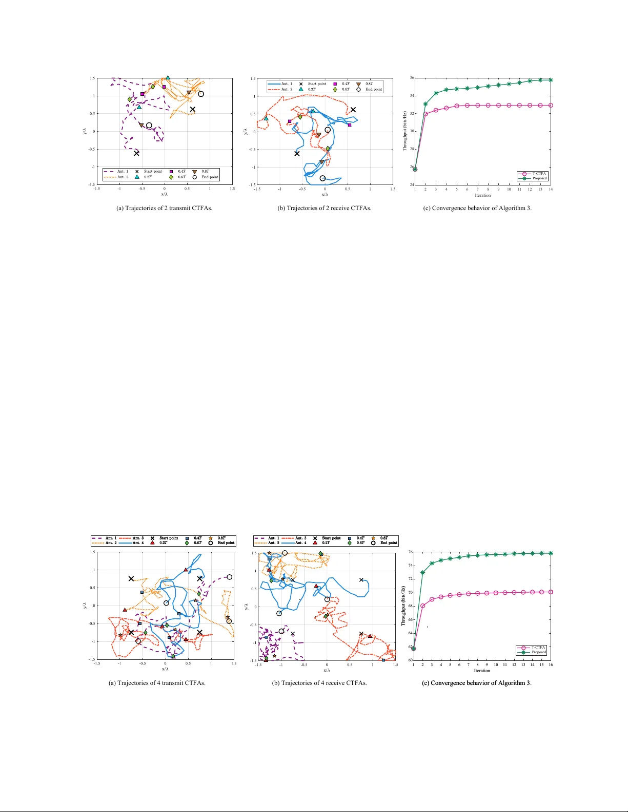
1 Antenna Elements’ T rajectory Optimization for Throughput Maximization in Continuous-T rajectory Fluid Antenna-Aided W ireless Communications Shuaixin Y ang, Y ijia Li, Y ue Xiao, Y ong Liang Guan, Kai-Kit W ong, Hyundong Shin, and Chau Y uen Abstract Fluid antenna (F A) systems offer no vel spatial de grees of freedom (DoFs) with the potential for significant performance gains. Compared to existing w orks focusing solely on optimizing F A positions at discrete time instants, we introduce the concept of continuous-trajectory fluid antenna (CTF A), which explicitly considers the antenna element’ s mov ement trajectory across continuous time intervals and incorporates the inherent kinematic constraints present in practical F A implementations. Accordingly , we formulate the total throughput maximization problem in CTF A-aided wireless communication systems, addressing the joint optimization of continuous antenna trajectories in conjunction with the transmit cov ariance matrices under kinematic constraints. T o effecti vely solve this non-con vex problem with highly coupled optimization variables, we de velop an iterativ e algorithm based on block coordinate S. Y ang, Y . Li and Y . Xiao are with the National K ey Laboratory of Wireless Communications, Univ ersity of Electronic Science and T echnology of China, Chengdu 611731, China (e-mail: shuaixin.yang@foxmail.com, nikoeric@foxmail.com, xiaoyue@uestc.edu.cn). Y . Guan and C. Y uen is with the School of Electrical and Electronic Engineering, Nanyang T echnological University , Singapore (e-mail: EYLGuan@ntu.edu.sg, chau.yuen@ntu.edu.sg.). K.-K. W ong is with the Department of Electronic and Electrical Engineering, University College London, WC1E 7JE London, U.K., and also with the Department of Electronic Engineering, Kyung Hee University , Y ongin-si, Gyeonggi-do 17104, Republic of Korea (e-mail: kai-kit.wong@ucl.ac.uk). H. Shin is with the Department of Electronics and Information Con ver gence Engineering, K yung Hee Univ ersity , 1732 Deogyeong-daero, Giheung-gu, Y ongin-si, Gyeonggi-do 17104, Republic of Korea (e-mail: hshin@khu.ac.kr). 2 descent (BCD) and majorization-minimization (MM) principles with the aid of the weighted minimum mean square error (WMMSE) method. Finally , numerical results are presented to validate the efficac y of the proposed algorithms and to quantify the substantial total throughput advantages afforded by the conceiv ed CTF A-aided system compared to con ventional fixed-position antenna (FP A) benchmarks and alternativ e approaches employing simplified trajectories. Index T erms Fluid antenna, continuous-trajectory fluid antenna (CTF A), trajectory optimization, multiple-input multiple-output (MIMO), kinematic constraints, block coordinate descent (BCD), majorization-minimization (MM). I . I N T RO D U C T I O N Sixth-generation (6G) wireless networks represent an en visioned paradigm shift, transcending con ventional communication frame works to deli ver ultra-reliable, lo w-latency , and intelligent connecti vity across heterogeneous and dynamic en vironments, including terrestrial, aerial, and spaceborne domains [1]. Achie ving this ambitious vision critically hinges upon fundamental physical layer innov ations, necessitating unprecedented levels of reconfigurability , adaptability , and deeply inte grated artificial intelligence (AI) capabilities [2], [3]. Among the key enabling technologies is the fluid antenna (F A), a nov el architecture offering the capability to dynamically reconfigure the antennas’ spatial position physically within a defined re gion. Such unique char- acteristic unlocks ne w de grees of freedom (DoFs), critically enhancing the potential for spatial di versity exploitation and communication performance optimization [4]–[8]. This fundamental capability of F A has spurred significant research interest. Building upon the pioneering insights presented in [6], recent research has further un veiled the versatility and sig- nificant advantages of F A systems over con ventional fixed-position antenna (FP A) architectures, primarily by exploiting dynamic antenna position adjustment. In particular , within the realm of physical layer security (PLS), the inherent spatial DoFs of F A have facilitated adv anced security strate gies. For instance, joint optimization of F A positions and transmit beamforming ef fecti vely maximizes secrecy rates, ev en under strict cov ertness constraints [9]. Furthermore, nov el coding-enhanced cooperativ e jamming techniques ensure interference is cancelable solely by the legitimate receiv er , enhancing secrecy via optimized port selection and power control [10]. Syner gistic combinations of F A with reconfigurable intelligent surfaces (RIS) hav e also demonstrated significant security augmentation, often ev aluated via secrecy outage probability 3 (SOP) analysis [11]–[13]. Complementing these designs, rigorous analyses under correlated fading deriv e compact expressions for av erage secrecy capacity (ASC), SOP , and secrecy energy ef ficiency (SEE), rev ealing F A ’ s advantages ov er traditional antenna div ersity schemes [14]. These benefits are further evidenced in complex multi-user non-orthogonal multiple access (NOMA)-based wireless po wered communication networks (WPCNs), quantifying ASC and SOP improv ements despite external and internal eavesdroppers [15]. Beyond security-oriented applications, F A has demonstrated its ability to enhance performance across various communication paradigms. For example, within cognitiv e radio (CR) networks, F A-equipped secondary users can adaptiv ely adjust their antenna positions to achiev e superior spectrum sensing accuracy , ef fectiv ely addressing stringent false-alarm constraints [16]. Similarly , in backscatter communication scenarios, F A deployed at the reader facilitates improv ed link reliability and reduces outage probability and delay outage rates by exploiting spatial DoFs [17]. Furthermore, integrating F A into wideband orthogonal frequency-di vision multiplexing (OFDM) systems, ex emplified by 5G New Radio (NR), has sho wn notable potential for throughput enhancement via adaptiv e modulation and strategic port selection tailored to frequency-selecti ve channel characteristics [18]. W ithin the emerging domain of integrated sensing and communi- cation (ISA C), F A technology provides novel av enues for managing the fundamental sensing- communication trade-of f via dynamic antenna configuration. Specifically , jointly optimizing F A positions and transmit precoding has been shown to maximize radar sensing signal-clutter-noise ratio (SCNR) under communication signal-to-interference-plus-noise ratio (SINR) constraints [19]. Furthermore, F A enables substantial transmit power minimization while satisfying both communication and sensing requirements, demonstrating flexibility in shifting the ISAC opera- tional point [20]. Extending this adaptability , jointly optimizing beamforming and F A positions at both the base station and user sides effecti vely maximizes downlink communication rates subject to stringent sensing gain requirements [21]. Despite the substantial body of research highlighting the theoretical adv antages and div erse applications of F A systems, there remains a notable gap between the predominantly adopted theoretical models and the practical realities of certain crucial hardware implementations, par- ticularly those based on mechanical actuation, such as motor-dri ven systems [22], [23]. The existing optimization framew orks and performance analyses typically assume an idealized sce- nario characterized by instantaneous and cost-fr ee switching among a set of predefined antenna port positions. Although this assumption provides significant analytical con venience, it ne ver - 4 theless neglects critical physical dynamics intrinsic to mechanically actuated antenna systems. A potential consequence is that performance predictions deri ved from such simplified models may deviate from those observed in practice, and optimization algorithms conceiv ed under these assumptions might require adaptation for deployment on motor -driv en F A platforms. More specifically , motor-based F A architectures, which inv olve the physical translation of antenna elements (AEs), introduce unique characteristics, notably the capability for continuous spatial mo vement. This property enables finer spatial sampling granularity and higher spatial res- olution, thereby f acilitating sophisticated trajectory-based optimization strate gies wherein antenna positions dynamically trace optimized trajectories corresponding to ev olving channel conditions. Ne vertheless, the inherent physical mov ements of such systems impose substantial dynamic factors fundamentally incompatible with the idealized instantaneous switching paradigm. These critical dynamics encompass significant motion delay (the finite duration required for antenna translation) and additional mechanical constraints (limitations on maximum v elocity , acceler- ation, and a vailable range of motion). Against this backdrop, sev eral insightful studies ha ve begun to incorporate mobility aspects. For instance, Ref. [24] primarily optimized trajectories to minimize physical reconfiguration time between positions subject to kinematic constraints, potentially neglecting trajectory op- timization during acti ve data transmission for communication enhancement. Additionally , Ref. [25] in vestigated mobile antennas on unmanned aerial vehicles (U A Vs), which generally pertains to macro-scale platform mobility rather than the micro-scale element repositioning germane to F As. Furthermore, the work in [26] explored six-dimensional mov able antennas (6DMAs), where the static three-dimensional (3D) positions and rotations of antenna surf aces are optimized to align with the long-term spatial user distribution, which is distinct from optimizing an antenna’ s continuous trajectory during acti ve transmission to lev erage instantaneous channel dynamics. Therefore, despite these initial efforts, a comprehensi ve framew ork fully capturing the physics of continuously moving antennas and facilitating joint communication-mobility optimization warrants further in vestigation. In this contribution, we specifically address F A systems capable of continuous physical move- ment by introducing the concept of continuous-trajectory fluid antenna (CTF A), explicitly incor- porating realistic kinematic constraints intrinsic to practical implementations. W ithin this CTF A frame work, we formulate the total throughput maximization problem, aiming at jointly optimizing the AEs’ continuous trajectory and the associated transmit co v ariance matrix (TCM) throughout 5 the communication session. Howe ver , as the AEs mov e along their continuous trajectories, the system may inevitably encounter deleterious deep fading conditions, while con versely identifying adv antageous positions characterized by the constructiv e superposition of multipath components. Therefore, the throughput-maximization trajectory design needs to effecti vely strik e an optimal balance between circumventing deep channel nulls and e xploiting f avourable propagation posi- tions. In a nutshell, the primary contributions of this paper are summarized as follo ws: • W e formulate a no vel joint antenna trajectory and TCM optimization problem under the CTF A frame work, explicitly incorporating practical channel characteristics and kinematic constraints during continuous motion. • W e dev elop an efficient alternating optimization algorithm, integrating block coordinate de- scent (BCD) and majorization-minimization (MM) principles, to find high-quality solutions for the formulated non-con ve x AE trajectory optimization problem. • W e demonstrate through numerical simulations that the proposed CTF A frame work, account- ing for realistic physical dynamics, yields significant performance improv ements compared to con ventional FP A systems and alternativ e approaches employing simplified trajectories. The remainder of this paper is structured as follo ws. Section II introduces the system model for CTF A systems and formulates the optimization problem for throughput maximization. Section III details the proposed BCD-MM-based algorithm. Section IV provides the simulation results to validate the proposed framework. Finally , Section V concludes the paper . . T r an s m it R eg io n C T F A Digital Sig n al Pro ce s s o r ... R F C h ain R F C h ain R F C h ain R F C h ain R F C h ain R F C h ain . R ec eiv e R e g io n C T F A Digital Sig n al Pro ce s s o r ... R F Ch a in R F Ch a in R F Ch a in R F Ch a in R F Ch a in R F Ch a in .. . .. . ... 1 2 t L ... 1 2 t L ... 1 2 r L Tr ansmit t e r Re c e ive r t x t y r x r y Σ Fig. 1. System model of the point-to-point CTF A-enabled MIMO system. Notation : Unless otherwise specified, bold lowercase and uppercase letters are used for column vectors and matrices, respectiv ely . C denotes the set of complex numbers. ( · ) T and ( · ) H denote 6 the transposition and Hermitian conjugate transposition, respectiv ely . tr( · ) , det( · ) , and rank( · ) denote the matrix trace, determinant, and rank operations, respecti vely . ∥ · ∥ 2 represents the Euclidean-2 norm for vectors. Re {·} takes the real part of a complex number . ∇ and ∇ 2 denote the gradient and Hessian operators, respecti vely . λ max ( · ) denotes the maximum eigen v alue of a matrix. diag( x ) returns a diagonal matrix with the elements of vector x on its main diagonal. I represents the identity matrix and X \ Y denotes the set of elements belonging to X but not to Y . A ⪰ 0 ( A ≻ 0 ) denotes that the matrix A is positi ve semidefinite (definite). I I . S Y S T E M M O D E L A N D P R O B L E M F O R M U L A T I O N A. System Model Fig. 1 portrays the system model conceiv ed for a point-to-point multiple-input multiple-output (MIMO) system incorporating CTF A. Specifically , the transmitter and recei ver are equipped with N t and N r AEs, respectiv ely . These elements are linked to the associated radio-frequenc y (RF) chains via flexible connectors, which facilitate the dynamic adjustment of antenna positions upon dedicated panels actuated by micro motors. For CTF A systems, the continuous antenna mov ement inherently induces time-varying antenna positions, which consequently giv es rise to time-varying channel characteristics. It is pertinent to emphasize that our analysis is predicated upon a quasi-static channel model, which is readily satisfied, for instance, if the operational duration is confined within the channel coherence interval or in scenarios where both the environmental scatterers and the transceiv er platforms remain stationary relativ e to the propagation en vironment. Therefore, we formulate a throughput expression that explicitly incorporates the continuous temporal antenna displacement, thereby setting the stage for the optimization strategies detailed subsequently . Firstly , we respecti vely denote Q ( τ ) ∈ C N t × N t and H ( τ ) ∈ C N r × N t as the time- v arying TCM and the channel matrix of CTF A systems to be elaborated in the next subsection. Then, the instantaneous achie vable rate can be expressed as R ( τ ) = log det  I + 1 σ 2 H ( τ ) Q ( τ ) H ( τ ) H  , (1) where Q ( τ ) satisfies the power constraint tr ( Q ( τ )) ≤ P and σ 2 denotes the variance of the additi ve white Gaussian noise (A WGN) at the receiv er . 7 Thus, the total throughput C that can be transmitted from the transmitter to the receiver ov er the duration T is expressed as C = Z T 0 log det  I + 1 σ 2 H ( τ ) Q ( τ ) H ( τ ) H  dτ . (2) B. Channel Model The channel characterizing the CTF A system is modeled based on the far -field multipath field-response framework detailed in [27], [28]. Explicitly , let L t and L r denote the number of dominant propagation paths associated with the transmitter and receiver , respectiv ely . The propa- gation delay incurred along the p -th transmit path ( p = 1 , 2 , . . . , L t ) is intrinsically dependent on the instantaneous positions of the transmit AEs, which is represented as q t ( τ ) = [ x t ( τ ) , y t ( τ )] T . Moreov er , the AEs are constrained to mov e within the square region C t = [0 , A ] × [0 , A ] , with the origin specified as o t = [0 , 0] T . Consequently , for the p -th transmit path, the position-dependent propagation offset ρ p t ( q t ( τ )) relativ e to the origin o t is formulated as ρ p t ( q t ( τ )) = x t ( τ ) sin θ p t cos ϕ p t + y t ( τ ) cos θ p t , (3) where θ p t and ϕ p t denote the corresponding elev ation and azimuth angles of departure (AoDs), respecti vely . Then, the phase shift incurred by the p -th transmit path is formulated as 2 π ρ p t ( q t ( τ )) /λ , where λ denotes the signal wa velength. Le veraging this phase shift formulation, the transmit field response v ector g ( q t ( τ )) associated with each transmit AE is constructed as g ( q t ( τ )) ≜ h e j 2 π λ ρ 1 t ( q t ( τ )) , e j 2 π λ ρ 2 t ( q t ( τ )) , . . . , e j 2 π λ ρ L t t ( q t ( τ )) i T . (4) Furthermore, letting ˜ q t ( τ ) ≜  q k t ( τ )  N t k =1 denote the collection of positions for all AEs at the BS, the composite field response matrix G ( ˜ q t ( τ )) incorporating all N t transmit AEs is defined as G ( ˜ q t ( τ )) ≜  g  q 1 t ( τ )  , g  q 2 t ( τ )  , . . . , g  q N t t ( τ )  . (5) Correspondingly , at the recei ver side, the elev ation and azimuth angles of arriv al (AoAs) associated with the q -th ( q = 1 , 2 , . . . , L r ) recei ve path are denoted by θ q r ∈ [0 , π ] and ϕ q r ∈ [0 , π ] , respecti vely . The resultant field response vector f ( q r ( τ )) for each receiv e AE positioned at q r ( τ ) = [ x r ( τ ) , y r ( τ )] T ∈ C r = [0 , A ] × [0 , A ] , is gi ven by f ( q r ( τ )) ≜ h e j 2 π λ ρ 1 r ( q r ( τ )) , e j 2 π λ ρ 2 r ( q r ( τ )) , . . . , e j 2 π λ ρ L r r ( q r ( τ )) i T , (6) 8 where ρ q r ( q r ( τ )) = x r ( τ ) sin θ q r cos ϕ q r + y r ( τ ) cos θ q r . Subsequently , the corresponding recei ve field response matrix is expressed as F ( ˜ q r ( τ )) ≜  f  q 1 r ( τ )  , f  q 2 r ( τ )  , . . . , f  q N r r ( τ )  , (7) where ˜ q r ( τ ) ≜  q l r ( τ )  N r l =1 . Furthermore, the path response matrix linking the reference points of the transmit and recei ve re gions, o t and o r , is denoted by Σ ∈ C L r × L t . Its elements, which capture the field response between the pertinent transmit and recei ve paths, are modeled as time- in variant independent and identically distributed (i.i.d.) complex random v ariables due to the assumption of a quasi-static channel. Additionally , we postulate a rich scattering en vironment, implying that min ( L t , L r ) ≥ max ( N t , N r ) . Based on the preceding definitions, the end-to- end MIMO channel matrix H ( τ ) characterizing the link between the transmitter and recei ver equipped with CTF As can finally be formulated as H ( τ ) = F ( ˜ q r ( τ )) H ΣG ( ˜ q t ( τ )) . (8) Evidently , the channel’ s temporal variations principally stem from the dynamic movement of the AEs. C. Kinematic Constraints In this subsection, we explicitly consider the kinematic constraints imposed on the CTF As. Specifically , the instantaneous velocities of the k -th transmit AE and l -th recei ve AE are obtained as the first deri vati ves of their respecti ve positions: v k t ( τ ) = d q k t ( τ ) dτ , ∀ k , ∀ τ , (9) v l r ( τ ) = d q l r ( τ ) dτ , ∀ l , ∀ τ . (10) Similarly , their corresponding instantaneous accelerations are deri ved as the second deriv ativ es of positions: a k t ( τ ) = d 2 q k t ( τ ) dτ 2 , ∀ k , ∀ τ , (11) a l r ( τ ) = d 2 q l r ( τ ) dτ 2 , ∀ l , ∀ τ . (12) 9 Owing to the inherent physical limitations of the actuating motors typically emplo yed in prac- tical CTF A implementations, constraints are imposed on the maximum achie vable velocity and acceleration. These limitations are modeled as   v k t ( τ )   2 ≤ V max , ∀ k , ∀ τ , (13)   v l r ( τ )   2 ≤ V max , ∀ l , ∀ τ , (14)   a k t ( τ )   2 ≤ a max , ∀ k , ∀ τ , (15)   a l r ( τ )   2 ≤ a max , ∀ l , ∀ τ , (16) where V max and a max denote the maximum v elocity and acceleration magnitudes, respectiv ely . D. Pr oblem F ormulation The objectiv e of this paper is to maximize the total throughput C in (2), which is achiev ed by jointly optimizing the AEs’ trajectories { ˜ q t ( τ ) , ˜ q r ( τ ) | 0 ≤ τ ≤ T } , v elocities { ˜ v t ( τ ) , ˜ v r ( τ ) | 0 ≤ τ ≤ T } , accelerations { ˜ a t ( τ ) , ˜ a r ( τ ) | 0 ≤ τ ≤ T } , and the TCMs { Q ( τ ) | 0 ≤ τ ≤ T } . Accordingly , the optimization problem is formulated as (P1) max Ω 1 C (17a) s.t. q k t ( τ ) ∈ C t , ∀ k , ∀ τ , (17b) q l r ( τ ) ∈ C r , ∀ l , ∀ τ , (17c)    q k t ( τ ) − q k ′ t ( τ )    2 ≥ D, k  = k ′ , ∀ τ , (17d)    q l r ( τ ) − q l ′ r ( τ )    2 ≥ D, l  = l ′ , ∀ τ , (17e) tr ( Q ( τ )) ≤ P , ∀ τ , (17f) Q ( τ ) ⪰ 0 , ∀ τ , (17g) (9) − (16) . where the set of optimization v ariables is Ω 1 = { Q ( τ ) , ˜ q t ( τ ) , ˜ q r ( τ ) , ˜ v t ( τ ) , ˜ v r ( τ ) , ˜ a t ( τ ) , ˜ a r ( τ ) | 0 ≤ τ ≤ T } , and D in (17d) and (17e) signifies the minimum distance between AEs within each time slot to mitigate potential coupling ef fects. Directly solving the optimization problem (P1) is intrinsically challenging, stemming from four primary impediments. First, it necessitates the optimization of continuous variables, namely 10 the AEs’ trajectories ˜ q ( τ ) , along with their associated first- and second-order deri vati ves (i.e., velocity ˜ v ( τ ) and acceleration ˜ a ( τ ) ), in conjunction with the transmit cov ariance matrix Q ( τ ) . This inherently constitutes an optimization problem within an infinite-dimensional functional space, rendering direct analytical or numerical solutions intractable. Second, the objectiv e func- tion in (P1) is formulated as an integral, which lacks a closed-form expression, precluding straightforward e valuation. Third, the problem’ s complexity is further compounded by the nature of the constraints. Specifically , the minimum distance constraints articulated in (17d) and (17e) are inherently non-con vex. Furthermore, the strong coupling among all optimization v ariables significantly exacerbates the difficulty of attaining a tractable solution for (P1) . T o enhance the tractability of the optimization problem (P1) , we utilize a discrete-time linear state-space approximation framew ork. This approach facilitates the deri v ation of the follo wing expressions, which are predicated upon first- and second-order T aylor series expansions under the stipulation of a suf ficiently small time step δ τ : ˜ v t ( τ + δ τ ) ≈ ˜ v t ( τ ) + ˜ a t ( τ ) δ τ , ∀ τ , (18) ˜ v r ( τ + δ τ ) ≈ ˜ v r ( τ ) + ˜ a r ( τ ) δ τ , ∀ τ , (19) ˜ q t ( τ + δ τ ) ≈ ˜ q t ( τ ) + ˜ v t ( τ ) δ τ + 1 2 ˜ a t ( τ ) δ 2 τ , ∀ τ , (20) ˜ q r ( τ + δ τ ) ≈ ˜ q r ( τ ) + ˜ v r ( τ ) δ τ + 1 2 ˜ a r ( τ ) δ 2 τ , ∀ τ . (21) Consequently , upon discretizing the time duration T into N + 1 slots, each of duration δ τ (i.e., sampling at time instants τ = nδ τ , n = 0 , 1 , · · · , N ), the continuous trajectory ˜ q t/r ( τ ) can be accurately characterized by the sequence of discrete-time AEs’ positions ˜ q t/r,n ≜ ˜ q t/r ( nδ τ ) . Similarly , the instantaneous v elocity and acceleration are represented by their discrete samples ˜ v t/r,n ≜ ˜ v t/r ( nδ τ ) and ˜ a t/r,n ≜ ˜ a t/r ( nδ τ ) , respectiv ely . Furthermore, the transmit cov ariance matrix is discretized as Q n ≜ Q ( nδ τ ) . This discretization, following the principles of [29], yields the subsequent discrete state-space model as ˜ v t,n +1 = ˜ v t,n + ˜ a t,n δ τ , ∀ n, (22) ˜ v r,n +1 = ˜ v r,n + ˜ a r,n δ τ , ∀ n, (23) ˜ q t,n +1 = ˜ q t,n + ˜ v t,n δ τ + 1 2 ˜ a t,n δ 2 τ , ∀ n, (24) ˜ q r,n +1 = ˜ q r,n + ˜ v r,n δ τ + 1 2 ˜ a r,n δ 2 τ , ∀ n. (25) 11 More explicitly , the validity of this discrete-time approximation relies on sev eral physical constraints. For the channel to remain approximately constant within each slot, the maximum dis- placement is required to be substantially smaller than a quarter -wav elength, which implies V max δ τ ≪ λ/ 4 . Furthermore, the first-order T aylor approximation of motion holds, provided that the velocity change a max δ τ is negligible compared to the maximum v elocity , leading to a max δ τ ≪ V max . Fi- nally , the underlying quasi-static channel assumption mandates that the total duration of T = N δ τ must be substantially smaller than the channel’ s coherence time T c , i.e., N δ τ ≪ T c . Hence, these constraints collectiv ely dictate that the slot duration δ τ must be chosen to satisfy δ τ ≪ min  T c N , λ 4 V max , V max a max  . Based upon the preceding mathematical manipulations, Problem (P1) can be reformulated as (P1 ′ ) max Ω 2 ˆ C (26a) s.t. q k t,n ∈ C t , ∀ k , ∀ n, (26b) q l r,n ∈ C r , ∀ l , ∀ n, (26c)    q k t,n − q k ′ t,n    2 ≥ D, k  = k ′ , ∀ n, (26d)    q l r,n − q l ′ r,n    2 ≥ D, l  = l ′ , ∀ n, (26e)   v k t,n   2 ≤ V max , ∀ k , ∀ n, (26f)   v l r,n   2 ≤ V max , ∀ l , ∀ n, (26g)   a k t,n   2 ≤ a max , ∀ k , ∀ n, (26h)   a l r,n   2 ≤ a max , ∀ l , ∀ n, (26i) tr ( Q n ) ≤ P , ∀ n, (26j) Q n ⪰ 0 , ∀ n, (26k) (22) − (25) . where Ω 2 = { Q n , ˜ q t,n , ˜ q r,n , ˜ v t,n , ˜ v r,n , ˜ a t,n , ˜ a r,n } N n =0 , (27) ˆ C = δ τ N X n =0 log det  I + 1 σ 2 H n Q n H H n  , (28) H n = F ( ˜ q r,n ) H ΣG ( ˜ q t,n ) . (29) 12 I I I . P R O P O S E D B C D - M M - B A S E D A L G O R I T H M In this section, we first reformulate (P1 ′ ) into a more tractable form. Then, the BCD-MM- based algorithm is proposed to alternately optimize the TCM matrices Q n , the AEs’ trajectories ˜ q t/r,n , velocities ˜ v t/r,n and accelerations ˜ a t/r,n . A. Pr oblem Reformulation and Optimization Addressing the intractability inherent in optimizing the objectiv e function of (P1 ′ ) , we in- vok e the well-established weighted minimum mean square error (WMMSE) algorithm [30]. This technique, commonly utilized for rate and sum-rate maximization problems, is specifically adapted herein to reformulate (P1 ′ ) . Fundamentally , the WMMSE approach transforms the original rate/sum-rate maximization objectiv e into an equiv alent and alternative formulation via the introduction of pertinent auxiliary variables. This reformulation is particularly advantageous as it renders the problem amenable to efficient optimization using BCD methods [31]. Such an idea is based on the result in the following lemma. Lemma 1. Define an m by m matrix function E ( U , V ) ≜  I − U H HV   I − U H HV  H + U H ZU , (30) wher e Z is any positive definite matrix. It holds true that log det  I + HVV H H H Z − 1  = max W ≻ 0 , U log det( W ) − tr( W E ( U , V )) + m. (31) The rigorous proof is provided in [30]. Subsequently , le veraging Lemma 1, an equiv alent formulation for the objecti ve function in (P1 ′ ) is deriv ed via the introduction of pertinent auxiliary v ariables { W n , U n } N n =0 . More specifically , let the matrix E n be defined as E n ≜  I − 1 σ U H n H n Q 1 2 n   I − 1 σ U H n H n Q 1 2 n  H + U H n U n , (32) where Q 1 2 n represents the matrix square root of Q n . Then, based on the WMMSE frame work, the throughput ˆ C admits the follo wing equi valent expression: ˆ C = δ τ N X n =0 log det  I + 1 σ 2 H n Q n H H n  = max { W n ≻ 0 , U n } N n =0 δ τ N X n =0 [log det ( W n ) − tr ( W n E n ) + N r ] . (33) 13 Neglecting the constant term and the overall scaling factor in the objecti ve function, neither of which affects the optimal solution, allo ws the problem to be reformulated as (P1 ′′ ) max Ω 3 h 1 ( Ω 3 ) (34a) s.t. W n ≻ 0 , (34b) (26b) − (26k) , (22) − (25) , where Ω 3 = { Q n , ˜ q t,n , ˜ q r,n , ˜ v t,n , ˜ v r,n , ˜ a t,n , ˜ a r,n , W n , U n } N n =0 , (35) h 1 ( Ω 3 ) = N X n =0 [log det ( W n ) − tr ( W n E n )] . (36) B. Optimize Q n This subsection addresses the optimization of the transmit cov ariance matrix Q n . Critically , gi ven fixed values for the other optimization variables, problem (P1 ′′ ) reduces to a con vex optimization problem with respect to Q n . By virtue of this con vexity , the optimal solution relies on the principles of eigenmode transmission. Specifically , let the truncated singular value decomposition (SVD) of H n be expressed as H n = M n Ξ n N H n , where M n ∈ C N r × S n and N n ∈ C N t × S n , and Ξ n ∈ C S n × S n is a diagonal matrix containing the S n ≜ rank ( H n ) non- zero singular v alues. Then, in voking the well-known water-filling solution, the optimal transmit cov ariance matrix Q ⋆ n can be obtained as Q ⋆ n = N n diag  p ⋆ 1 , p ⋆ 2 , . . . , p ⋆ S n  N H n , (37) where p ⋆ s = max (0 , 1 /µ − σ 2 / Ξ n [ s, s ] 2 ) , and µ is the water -lev el chosen to satisfy P S n s =1 p ⋆ s = P . C. Optimize U n and W n Observe that the expression in Eq. (34a) exhibits concavity with respect to both W n and U n when the remaining variables are held constant. Consequently , this property permits the application of the first-order optimality condition, yielding the optimal solutions for W n and U n as follows. 14 Theorem 2. The optimal solutions of W n and U n ar e given by U ⋆ n = arg max U n h 1 ( Ω 3 ) = 1 σ  I + 1 σ 2 H n Q n H H n  − 1 H n Q 1 2 n , (38) and W ⋆ n = arg max W n ≻ 0 h 1 ( Ω 3 ) = "  I − 1 σ U ⋆H n H n Q 1 2 n   I − 1 σ U ⋆H n H n Q 1 2 n  H + U ⋆H n U ⋆ n # − 1 . (39) Pr oof. See Appendix A. D. Optimize  q k t,n , v k t,n , a k t,n  N n =0 The focus of this subsection pertains to optimizing the sequence variables representing the k -th transmit AE’ s position q k t,n , velocity v k t,n , and acceleration a k t,n across all time indices n = 0 , 1 , . . . , N . T o this end, the pertinent subproblem deri ved from (P1 ′′ ) is reformulated as (P2 - k) min Ω 4 h 2  q k t  (40a) s.t. (26b) , (26d) , (26f) , (26h) , (22) , (24) . where Ω 4 =  q k t,n , v k t,n , a k t,n  N n =0 , (41) h 2  q k t  = N X n =0 tr ( W n E n ) . (42) Problem (P2 - k) is notably intractable, primarily attributed to two factors: firstly , the pronounced non-con ve xity of the objecti ve function with respect to the optimization variables  q k t,n , v k t,n , a k t,n  N n =0 , and secondly , the coupled relationships among the v ariables within the constraints, which, particularly due to the minimum distance constraint (26d), results in a non-con ve x feasible region. T o address the challenges delineated abov e, we first focus on reformulating the objecti ve function of (P2 - k) into a mathematically more tractable form. Owing to the uniform structure exhibited by the summation terms within h 2  q k t  , it suf fices, without loss of generality , to analyze 15 a single representati ve term corresponding to the time index n within it. Specifically , in voking the channel matrix definitions provided in (8), we establish the following theorem. Theorem 3. tr ( W n E n ) = g  q k t,n  H B k t,n g  q k t,n  + 2Re n g  q k t,n  H d k t,n o + const , (43) wher e Q H 2 n = h b 1 X,n b 2 X,n · · · b N t X,n i , (44) B k t,n ≜  b k X,n  H b k X,n C t,n , (45) C t,n ≜ 1 σ 2 Σ H F ( ˜ q r,n ) U n W n U H n F ( ˜ q r,n ) H Σ , (46) d k t,n ≜ C t,n " N t X i =1 ,i  = k g  q i t,n   b i X,n  H # b k X,n − α k t,n , (47) A t,n ≜ 1 σ Σ H F ( ˜ q r,n ) U n W n Q H 2 n (48) = h α 1 t,n α 2 t,n · · · α N t t,n i . Pr oof. See Appendix B. Thus, (P2 - k) can be reformulated as (P2 ′ - k) min Ω 4 h 3  q k t  (49a) s.t. (26b) , (26d) , (26f) , (26h) , (22) , (24) . where h 3  q k t  = N X n =0 h g ( q k t,n ) H B k t,n g ( q k t,n )+ 2Re { g ( q k t,n ) H d k t,n } i | {z } ≜ H 3 ( q k t,n ) . (50) The non-con vexity of problem (P2 ′ - k) , arising from both its objectiv e function and constraints, necessitates an iterativ e solution approach. Henceforth, the MM algorithm [32] is in voked to circumvent this intractability . Specifically , owing to the structural consistency of the summation terms within the objectiv e function, our analysis focuses, without loss of generality , on the representati ve constituent term H 3  q k t,n  . Let q k, ( i ) t,n denote the solution obtained for the antenna 16 position at the i -th iteration, with the corresponding objectiv e function v alue being H 3  q k, ( i ) t,n  . The MM algorithm proceeds by iterativ ely minimizing a surrogate function. Accordingly , at the ( i + 1) -th iteration, it is required to construct a surrogate function γ  q k t,n  that satisfies the three subsequent conditions: • γ  q k, ( i ) t,n  = H 3  q k, ( i ) t,n  , • ∇ γ  q k, ( i ) t,n  = ∇H 3  q k, ( i ) t,n  , • γ  q k t,n  ≥ H 3  q k t,n  . T o construct the surrogate function, an upper bound for the first summation term in H 3  q k, ( i ) t,n  is giv en as follo ws. Lemma 4. g ( q k t,n ) H B k t,n g ( q k t,n ) ≤ g ( q k t,n ) H Φ k t,n g ( q k t,n ) − 2 Re n g ( q k t,n ) H  Φ k t,n − B k t,n  g ( q k, ( i ) t,n ) o + g ( q k, ( i ) t,n ) H  Φ k t,n − B k t,n  g ( q k, ( i ) t,n ) = L t λ max  B k t,n  + g ( q k, ( i ) t,n ) H  Φ k t,n − B k t,n  g ( q k, ( i ) t,n ) | {z } const − 2 Re n g ( q k t,n ) H  Φ k t,n − B k t,n  g ( q k, ( i ) t,n ) o | {z } ≜ µ t ( q k t,n ) , (51) wher e Φ k t,n = λ max  B k t,n  I . Pr oof. Please refer to [33]. According to Lemma 4 and ignoring the constant terms, the surrogate function of H 3  q k, ( i ) t,n  can be constructed as τ t  q k t,n  ≜ µ t  q k t,n  + 2 Re n g ( q k t,n ) H d k t,n o = 2 Re n g ( q k t,n ) H η k, ( i ) t,n o , (52) where η k, ( i ) t,n = d k t,n −  Φ k t,n − B k t,n  g ( q k, ( i ) t,n ) . (53) Although Eq. (52) exhibits linearity with respect to the field response vector g ( q k t,n ) , it nonethe- less remains non-con vex and non-conca ve with respect to the AE’ s position q k t,n . This characteris- tic precludes straightforward con vex optimization techniques. Therefore, we resort to employing 17 the second-order T aylor expansion for constructing the surrogate function of τ t  q k t,n  , which is gi ven by τ t  q k t,n  ≤ τ t  q k, ( i ) t,n  + ∇ τ t  q k, ( i ) t,n  T  q k t,n − q k, ( i ) t,n  + δ k t,n 2  q k t,n − q k, ( i ) t,n  T  q k t,n − q k, ( i ) t,n  = δ k t,n 2  q k t,n  T q k t,n + ( ∇ τ t  q k, ( i ) t,n  − δ k t,n q k, ( i ) t,n ) T q k t,n | {z } ≜ γ t ( q k t,n ) + τ t  q k, ( i ) t,n  + δ k t,n 2  q k, ( i ) t,n  T q k, ( i ) t,n − ∇ τ t  q k, ( i ) t,n  T q k, ( i ) t,n | {z } const , (54) where δ k t,n is a positive real number satisfying δ k t,n I ⪰ ∇ 2 τ t  q k t,n  . Follo wing similar deriv ations in [34], the gradient vector ∇ τ t  q k t,n  and the Hessian matrix ∇ 2 τ t  q k t,n  with respect to (w .r .t.) q k t,n are giv en in Appendix D, and the construction of δ k t,n is presented in Appendix E. Therefore, with the aid of all the surrogate functions γ t  q k t,n  , n = 0 , 1 , · · · , N , (P2 ′ - k) can be approximated as (P2 ′′ - k) min Ω 4 N X n =0 γ t  q k t,n  (55a) s.t. (26b) , (26d) , (26f) , (26h) , (22) , (24) . which is still non-con vex owing to the constraint (26d). Here, we resort to obtaining a sub- optimal local maximum by applying con ve x relaxation to constraint (26d). More precisely , by conducting the first-order T aylor e xpansion of the con vex function with respect to q k t,n , we can deri ve a lower bound of   q k t,n − q k ′ t,n   2 as    q k t,n − q k ′ t,n    2 ≥  ∇    q k, ( i ) t,n − q k ′ t,n    2  T  q k t,n − q k, ( i ) t,n  +    q k, ( i ) t,n − q k ′ t,n    2 =  q k, ( i ) t,n − q k ′ t,n  T    q k, ( i ) t,n − q k ′ t,n    2  q k t,n − q k ′ t,n  , (56) 18 thereby allowing con ve x relaxation of the constraint (26d) to  q k, ( i ) t,n − q k ′ t,n  T    q k, ( i ) t,n − q k ′ t,n    2  q k t,n − q k ′ t,n  ≥ D, (57) and furthermore, the subproblem (P2 ′′ - k) can be transformed into (P2 ′′′ - k) min Ω 4 N X n =0 γ t  q k t,n  (58a) s.t.  q k, ( i ) t,n − q k ′ t,n  T    q k, ( i ) t,n − q k ′ t,n    2  q k t,n − q k ′ t,n  ≥ D, k  = k ′ , (58b) (26b) , (26f) , (26h) , (22) , (24) , which is a con ve x quadratically constrained quadratic programming (QCQP) problem and can be ef ficiently solved using cvx. The details of the MM algorithm for solving problem (P2-k) are summarized in Algorithm 1. Algorithm 1 MM Algorithm for Solving (P2 - k) Input: Σ , N t , N r , L r , L t , { θ p t } L t p =1 , { ϕ p t } L t p =1 , { θ q r } L r q =1 , { ϕ q r } L r q =1 , C t , C r , D , ϵ . Output:  q k t,n , v k t,n , a k t,n  N n =0 . 1: Initialization: i = 0 . 2: Obtain Φ k t,n according to Lemma 4; 3: while Relativ e decrease of h 2  q k t,n  is above ϵ do 4: Obtain η k, ( i ) t,n according to (53); 5: Obtain ∇ τ t  q k t,n  and ∇ 2 τ t  q k t,n  according to Appendix D; 6: Obtain δ k t,n according to (101); 7: Obtain n q k, ( i +1) t,n , v k, ( i +1) t,n , a k, ( i +1) t,n o N n =0 by solving (P2 ′′′ - k) ; 8: i = i + 1 ; 9: end while Next, we analyze the con ver gence of the proposed Algorithm 1. Denote the two constant terms in (54) and (51) by Γ t, 1  q k, ( i ) t,n  and Γ t, 2  q k, ( i ) t,n  . Then, for the i -th iteration, the objectiv e 19 function in (P2 ′ - k) can be written as N X n =0 H 3  q k, ( i ) t,n  ( a ) = N X n =0 γ t  q k, ( i ) t,n  + N X n =0 Γ t, 1  q k, ( i ) t,n  + N X n =0 Γ t, 2  q k, ( i ) t,n  ( b ) ≥ N X n =0 γ t  q k, ( i +1) t,n  + N X n =0 Γ t, 1  q k, ( i ) t,n  + N X n =0 Γ t, 2  q k, ( i ) t,n  ( c ) ≥ N X n =0 τ t  q k, ( i +1) t,n  + N X n =0 Γ t, 2  q k, ( i ) t,n  ( d ) ≥ N X n =0 H 3  q k, ( i +1) t,n  , (59) where the equality marked by (a) holds because the expansion in (54) and (51) are tight at q k, ( i ) t,n . The inequality marked by (b) holds because we minimize the v alue of γ t  q k t,n  in the i -th iteration, and the equality can be achie ved by choosing ˜ q ( i +1) t,n = ˜ q ( i ) t,n . The inequalities denoted by (c) and (d) are satisfied o wing to the fact that γ t  q k t,n  + Γ t, 1  q k, ( i ) t,n  and τ t  q k t,n  + Γ t, 2  q k, ( i ) t,n  constitute the constructed surrogate functions for τ t  q k t,n  and H 3  q k t,n  , respecti vely . A direct consequence of this surrogate function construction is that the sequence of objectiv e function v alues n h 3  q k, ( i ) t o + ∞ i =0 is guaranteed to be non-increasing, and therefore, it con verges to a stationary point, specifically a minimum value in this conte xt. The computational complexity of the conceiv ed algorithm is detailed as follo ws. Initially , in Step 2, the determination of the maximum eigen value of the matrix B k t,n , typically achiev ed via eigen value decomposition, incurs a complexity on the order of O ( L 3 t ) . Subsequently , in Step 4, the calculation of η k, ( i ) t,n requires O ( L 2 t ) operations. Furthermore, the complexities associated with obtaining the gradient ∇ τ t  q k, ( i ) t,n  , the Hessian ∇ 2 τ t  q k, ( i ) t,n  , and the scalar δ n t,k in Steps 5 and 6 are O ( L t ) , O ( L t ) , and O (1) , respecti vely . Finally , in Step 7, solving the con vex QCQP subproblem (P5-m) using an interior-point method [35] to attain an accurac y of β exhibits a complexity of O ( N 3 . 5 log(1 /β )) . Let I t denote the maximum number of iterations required for con ver gence of the loop comprising Steps 4-7. Therefore, the overall computational complexity of Algorithm 1 is dominated by O ( L 3 t + I t ( L 2 t + N 3 . 5 log(1 /β ))) . 20 E. Optimize  q l r,n , v l r,n , a l r,n  N n =0 The optimization objecti ve within this subsection is focused on the l -th receiv e AE, specif- ically determining its position q l r,n , velocity v l r,n , and acceleration a l r,n for all time indices n . Consequently , the rele vant subproblem is reformulated as (P3 - l) min Ω 5 h 4  q l r  (60a) s.t. (26c) , (26e) , (26g) , (26i) , (23) , (25) . where Ω 5 =  q l r,n , v l r,n , a l r,n  N n =0 , (61) h 4  q l r  = N X n =0 tr ( W n E n ) . (62) T o facilitate the subsequent analysis and render the formulation more tractable, the following theorem, which is analogous to Theorem 3, is established as follo ws. Theorem 5. tr ( W n E n ) = f  q l r,n  H B l r,n f  q l r,n  + 2Re n f  q l r,n  H d l r,n o + const , (63) wher e L X,n ≜ U n W n U H n , (64) L H 2 X,n = h l 1 X,n l 2 X,n · · · l N r X,n i , (65) B l r,n ≜  l l X,n  H l l X,n C r,n , (66) C r,n ≜ 1 σ 2 ΣG ( ˜ q t,n ) Q n G ( ˜ q t,n ) H Σ H , (67) d l r,n ≜ C r,n " N r X i =1 ,i  = l f  q i r,n   l i X,n  H # l l X,n − α l r,n , (68) A r,n ≜ 1 σ ΣG ( ˜ q t,n ) Q 1 2 n W H n U H n (69) = h α 1 r,n α 2 r,n · · · α N r r,n i . Pr oof. See Appendix C. 21 Follo wing a similar procedure, by defining τ r  q l r,n  ≜ 2 Re n f ( q l r,n ) H η l, ( i ) r,n o , where η l, ( i ) r,n ≜ d l r,n −  Φ l r,n − B l r,n  f ( q l, ( i ) r,n ) (70) with Φ l r,n = λ max  B l r,n  I , (71) the surrogate function can be constructed as P N n =0 γ r  q l r,n  , where γ r  q l r,n  ≜ δ l r,n 2  q l r,n  T q l r,n + ( ∇ τ r  q l, ( i ) r,n  − δ l r,n q l r,n ) T q l r,n with δ l r,n I ⪰ ∇ 2 τ r  q l r,n  . In addition, the con vex relaxation of the constraint (26e) can be obtained as  q l, ( i ) r,n − q l ′ r,n  T    q l, ( i ) r,n − q l ′ r,n    2  q l r,n − q l ′ r,n  ≥ D. (72) Finally , the subproblem (P3-l) can be transformed into (P3 ′ - l) min Ω 5 N X n =0 γ r  q l r,n  (73a) s.t.  q l, ( i ) r,n − q l ′ r,n  T    q l, ( i ) r,n − q l ′ r,n    2  q l r,n − q l ′ r,n  ≥ D, l  = l ′ , (73b) (26c) , (26g) , (26i) , (23) , (25) . which is a con ve x QCQP problem as well. The details of the MM algorithm for solving problem (P3 - l) are summarized in Algorithm 2. Similar to the analysis in Section III-D, the monotonic con vergence is guaranteed for solving problem (P3 - l) with Algorithm 2. The corresponding computational complexity is O  L 3 r + I r ( L 2 r + N 3 . 5 log(1 /β ))  , with I r denoting the maximum number of iterations to perform steps 4-6. F . Overall Algorithm Building upon the preceding analysis, the concei ved BCD-MM framew ork for addressing problem (P1 ′ ) is now completed. The overall algorithmic procedure is delineated in Algorithm 3. Specifically , Steps 3 through 7 encompass the sequential optimization of the N TCMs and the two pertinent WMMSE auxiliary v ariables, according to (37), (38), and (39), respectiv ely . Subsequently , during Steps 8 to 10, the positions of the N t transmit AEs are sequentially optimized by solving problem (P2 ′′′ - k) le veraging the MM approach. Analogously , in Steps 11 to 22 Algorithm 2 MM Algorithm for Solving Problem (P3 - l) Input: Σ , N t , N r , L r , L t , { θ p t } L t p =1 , { ϕ p t } L t p =1 , { θ q r } L r q =1 , { ϕ q r } L r q =1 , C t , C r , D , ϵ . Output:  q l r,n , v l r,n , a l r,n  N n =0 . 1: Initialization: i = 0 . 2: Obtain Φ l r,n according to (71); 3: while Relativ e decrease of h 4  q l r,n  is above ϵ do 4: Obtain η l, ( i ) r,n according to (70); 5: Obtain ∇ τ r  q l, ( i ) r,n  , ∇ 2 τ r  q l, ( i ) r,n  and δ l r,n as in [34]; 6: Obtain n q l, ( i +1) r,n , v l, ( i +1) r,n , a l, ( i +1) r,n o N n =0 by solving (P3 ′ - l) ; 7: i = i + 1 ; 8: end while 13, the positions of the N r recei ve AEs are iterati vely optimized via the solution of subproblem (P3 ′ - l) , again employing the MM algorithm. The algorithm iterates among these constituent subproblem solutions until con ver gence is attained, which is signified by the incremental increase in the v alue of h 1 ( Ω 3 ) falling belo w a predefined tolerance threshold ϵ . It should be noted that the sequential nature of Algorithm 3 is a characteristic of the BCD-based computational method. In the actual physical implementation, all antenna elements execute their computed optimal trajectories in parallel. The con ver gence characteristics of Algorithm 3 are analyzed as follows. By virtue of the BCD approach combined with the MM principle applied to its subproblems, the sequence of objectiv e function values generated for problem (P1 ′ ) is ensured to be monotonically non-decreasing across consecuti ve iterations. Furthermore, this sequence of objecti ve values is intrinsically upper - bounded due to the finite nature of the underlying throughput. Consequently , Algorithm 3 is guaranteed to con ver ge to at least a locally optimal solution for the reformulated problem (P1 ′ ) . In the following, the computational complexity of Algorithm 3 is analyzed. Initially , the computation of the optimal transmit covariance matrices Q n via water -filling in Step 4 typically requiring an SVD incurs a complexity of O ( N r N t min ( N r , N t )) . Subsequently , the determi- nation of the auxiliary matrices U n and W n in Steps 5-6 exhibits complexities of O ( N 3 r ) and O ( N 3 t ) , respecti vely . It is pertinent to note that these updates in Steps 4-6 are ex ecuted N times within each iteration of the main BCD loop. Furthermore, optimizing the transmit 23 Algorithm 3 Alternating Optimization for Solving Problem (P1 ′ ) Input: Σ , N t , N r , L r , L t , { θ p t } L t p =1 , { ϕ p t } L t p =1 , { θ q r } L r q =1 , { ϕ q r } L r q =1 , C t , C r , D , ϵ . Output: { Q n , ˜ q t,n , ˜ q r,n , ˜ v t,n , ˜ v r,n , ˜ a t,n , ˜ a r,n , W n , U n } N n =0 . 1: Initialization. 2: while Relativ e increase of h 1 ( Ω 3 ) is abo ve ϵ do 3: f or n = 0 → N do 4: Gi ven Ω 3 \ { Q n } , update Q n via (37); 5: Gi ven Ω 3 \ { U n } , update U n via (38); 6: Gi ven Ω 3 \ { W n } , update W n via (39); 7: end for 8: f or k = 1 → N t do 9: Gi ven Ω 3 \  q k t,n , v k t,n , a k t,n  N n =0 , solve (P2 - k) to update  q k t,n , v k t,n , a k t,n  N n =0 ; 10: end for 11: f or l = 1 → N r do 12: Gi ven Ω 3 \  q l r,n , v l r,n , a l r,n  N n =0 , solve (P3 - l) to update  q l r,n , v l r,n , a l r,n  N n =0 ; 13: end for 14: end while F A trajectory v ariables  q k t,n , v k t,n , a k t,n  N +1 n =0 in Steps 8-10 via Algorithm 1 and the recei ve F A trajectory variables  q k r,n , v k r,n , a k r,n  N +1 n =0 in Steps 11-13 via Algorithm 2 are associated with com- plexities of O ( N t L 3 t + N t I t ( L 2 t + N 3 . 5 log(1 /β ))) and O ( N r L 3 r + N r I r ( L 2 r + N 3 . 5 log(1 /β ))) , respecti vely , where I t and I r denote the maximum inner MM iteration counts. Therefore, letting I out be the maximum number of outer BCD iterations, the ov erall computational complex- ity of Algorithm 3 is dominated by O (( N N r N t min ( N r , N t ) + N N 3 t + N N 3 r + N t L 3 t + N r L 3 r + N t I t  L 2 t + N 3 . 5 log 1 β  + N r I r  L 2 r + N 3 . 5 log 1 β  I out  . I V . S I M U L A T I O N R E S U LT S This section presents simulation results conceiv ed both to v alidate the efficac y of the proposed algorithm and to demonstrate the throughput adv antages af forded by CTF A systems over con ven- tional FP A arrangements. In our simulation setup, we stipulate a signal-to-noise ratio (SNR) of 10 dB and employ a carrier frequency of 7.5 GHz, reflecting propagation conditions encountered at higher frequencies. T o ensure practical relev ance, the kinematics of the CTF As are constrained 24 such that the maximum velocity is limited to 0 . 016 m / s and the maximum acceleration is capped at 0 . 6 m / s 2 [22], [23]. Furthermore, the operational area for antenna movement is confined to a square re gion having a side length of A = 3 λ . Regarding the multipath channel model, we assume L t = L r = 5 paths between the transceiv ers. The path response matrix is modeled as Σ = diag ( α 1 , · · · , α L t ) . Denoting the Rician factor K as the ratio of the a verage po wer for line-of-sight (LoS) paths to that for non-line-of-sight (NLoS) paths, the path gains for the NLoS case ( K = 0 ) follow α l ∼ C N (0 , 1 /L t ) , while for LoS scenarios ( K > 0 ), they follo w α 1 ∼ C N  0 , K K +1  and α l ∼ C N  0 , 1 ( K +1)( L t − 1)  for l ≥ 2 . Additionally , the physical AoDs and AoAs are modeled as i.i.d. random v ariables, each uniformly distrib uted over the interval [0 , π ] . Finally , a minimum inter-AE distance of D = λ/ 2 is imposed to mitigate potential mutual coupling effects. The performance of Algorithm 3 is compared with fi ve benchmark schemes: 1) T ransmit CTF A (T -CTF A): The receiv er is equipped with an FP A-based uniform planar array (UP A), while the transmitter employs CTF As. In other words, Algorithm 3 is in voked only for the alternating optimization of the remaining variables in Ω 3 \ { ˜ q r,n , ˜ v r,n , ˜ a r,n } N n =0 . 2) Linear trajectory I: While maintaining identical original and final antenna positions as the proposed scheme, this baseline trajectory deviates from our total-throughput optimized solution, employing instead a uniform linear motion trajectory . 3) Linear trajectory II: In this scheme, the final antenna position is deri ved through instanta- neous rate optimization, as detailed in [27]. Furthermore, the antenna trajectory follo ws a uniform linear motion trajectory . 4) Random trajectory: In this baseline configuration, both the trajectory and the final antenna position are randomly generated; howe ver , the generated trajectory is constrained to adhere to the stipulations outlined in (9)-(16) and (17b)-(17g). 5) FP A: This con ventional benchmark employs FP A-based UP As at both the transmitter and recei ver . Consequently , within the optimization frame work, only the transmit covariance matrices { Q n } N n =0 are subject to optimization. Figs. 2(a), (b), and (c) illustrate the optimized trajectories of the transmit and recei ve AEs, along with the con ver gence curve, within the 2 × 2 CTF A system. As depicted in (a) and (b), the antennas exhibit a tendency towards intricate movements to enhance the total throughput. T o visualize the optimization process, distinct markers are employed to indicate the antenna positions at different time instants. It can be observed that the antennas continuously adjust 25 1 2 3 4 5 6 7 8 9 10 11 12 13 14 I ter atio n 24 26 28 30 32 34 36 T - CT F A P ropos e d (a ) T raje cto r ies o f 2 trans m it CTF As. (b) Tr ajectorie s o f 2 r eceive CT FAs. (c ) Co n v er g e n c e beh av io r of A lg o rithm 3. Thro u g h p u t ( b it s/ Hz) Fig. 2. Simulation results for the 2 × 2 CTF A system. their positions from the start point ( × ) to the end point ( ◦ ) to dynamically adapt to the channel en vironment. This beha vior is attrib uted, in part, to the constraints imposed by the minimum antenna separation and kinematic limitations, which restrict the DoFs in antenna motion. Fur- thermore, these complex trajectories are also indicativ e of the optimization process’ s endeav or to circumvent local optima, thereby unlocking greater performance potential. Fig. 2(c) illustrates the con vergence performance of Algorithm 3, re vealing that both the transmit CTF A scheme and the proposed scheme exhibit rapid con ver gence to their respecti ve optimal v alues within 14 iterations. This rapid con vergence underscores the efficienc y of our proposed algorithm. Quantitati vely , in comparison to their respectiv e initial v alues, the optimized solutions achiev ed by the two schemes demonstrate substantial performance enhancements of 38 . 6% and 15 . 9% , respecti vely . (a ) T ra je cto r ies of 4 tra n sm it CT F As. (b) Tr ajec to rie s o f 4 r ece iv e CT FAs. 1 2 3 4 5 6 7 8 9 10 11 12 13 14 15 16 I ter atio n 60 62 64 66 68 70 72 74 76 T - CT F A P ropos e d (c ) Co n v er g e n c e b ehav ior of A lg o rit h m 3 . Thro u g h p u t ( b it s/ Hz) 1 2 3 4 5 6 7 8 9 10 11 12 13 14 15 16 I ter atio n 60 62 64 66 68 70 72 74 76 T - CT F A P ropos e d (c ) Co n v er g e n c e b ehav ior of A lg o rit h m 3 . Thro u g h p u t ( b it s/ Hz) Fig. 3. Simulation results for the 4 × 4 CTF A system. 26 Figs. 3(a), (b), and (c) present simulation results for the 4 × 4 CTF A system. In contrast to the results in Fig. 2, Fig. 3(a) and (b) rev eal more intricate antenna movement patterns. This increased complexity arises from the constrained mov ement area and the heightened probability of antenna collisions, necessitating more sophisticated trajectory planning to achie ve a superior compromise between physical limitations and performance. It is crucial to emphasize, howe ver , that this challenge can be readily addressed by expanding the mo vement area. At higher carrier frequencies, this trade-of f becomes negligible, as achie ving ideal performance typically requires an area side length commensurate with the wa velength scale. Fig. 3(c) illustrates the con vergence performance of Algorithm 3 within this 4 × 4 system, exhibiting a rapid con ver gence characteristic akin to that observed in Fig. 2(c). This consistent con ver gence behavior suggests that our algorithm is not unduly sensiti ve to the increase in the number of antennas, highlighting its potential for low-comple xity operation e ven in larger -scale antenna configurations. Within the 4 × 4 system, both the transmit CTF A and the proposed schemes demonstrate performance improv ements of approximately 11 . 6% and 22 . 6% , respectiv ely , relati ve to their initial values. This marginal reduction in performance gains is attributed to the further constrained DoFs in antenna movement. T ABLE I C O M PA R I S O N O F T O T A L T H R O U G H P U T A N D P E R C E N TAG E G A I N O V E R F P A F O R D I FF E R E N T S C H E M E S . Configuration Metric Proposed T ransmit CTF A Linear trajectory I Linear trajectory II Random trajectory FP A 2 × 2 Throughput (bits/Hz) 35 . 76 32 . 92 28 . 79 27 . 48 25 . 9 27 . 06 Gain over FP A 32 . 15% 21 . 66% 6 . 39% 1 . 55% − 4 . 29% − 4 × 4 Throughput (bits/Hz) 75 . 82 70 . 09 67 . 10 66 . 17 55 . 18 58 . 40 Gain over FP A 29 . 83% 19 . 98% 14 . 89% 13 . 30% − 5 . 51% − T able I presents a comparativ e analysis of the total throughput attained by the various schemes. Se veral salient trends warrant highlighting: Firstly , the results confirm the universal performance enhancement of CTF A technology . All e valuated CTF A-based schemes consistently outperform the con ventional FP A benchmark, unequi vocally validating the intrinsic adv antage of le verag- ing antenna mobility to mitigate fading via additional spatial DoFs. Secondly , the paramount importance of joint trajectory and transmit cov ariance optimization is evident. Our proposed scheme achiev es the highest throughput in both 2 × 2 and 4 × 4 configurations, representing substantial gains of 32.15% and 29.83% ov er the FP A baseline. These gains substantiate the 27 T ABLE II S E N S I T I V I T Y A N A L Y S I S O F C O N V E R G E N C E A N D T H R O U G H P U T U N D E R D I FF E R E N T C H A N N E L C O N D I T I O N S . Fixed L = 5 NLoS, K = 0 LoS, K = 1 LoS, K = 5 LoS, K = 10 2 × 2 Iterations 14 13 16 11 Throughput (bits/Hz) 35 . 76 30 . 23 25 . 93 24 . 27 4 × 4 Iterations 16 46 36 10 Throughput (bits/Hz) 75 . 82 67 . 18 55 . 32 48 . 92 Fixed NLoS L = 5 L = 10 L = 15 L = 20 2 × 2 Iterations 14 5 5 7 Throughput (bits/Hz) 35 . 76 34 . 84 29 . 77 37 . 49 4 × 4 Iterations 16 24 16 29 Throughput (bits/Hz) 75 . 82 56 . 53 68 . 02 62 . 31 ef ficacy of our joint optimization strate gy . Notably , the proposed scheme significantly surpasses benchmarks relying on simplified uniform linear motion, indicating that meticulous optimiza- tion of the entire trajectory is crucial for maximizing CTF A performance. Thirdly , the MIMO configuration influences the gain magnitude, yet CTF A advantages remain significant. Although the relativ e gain is marginally lower in the 4 × 4 scenario (29.83%) versus 2 × 2 case (32.15%), attributable to tighter constraints from more antennas limiting positioning freedom, the absolute performance improv ement remains considerable, corroborating CTF A ’ s value in complex multi- antenna systems. Furthermore, linear trajectory I consistently outperforms linear trajectory II, which suggests that le veraging ev en partial trajectory information, i.e., the optimized endpoints, yields better results than optimizing solely for the final position, reinforcing the importance of the trajectory , although both linear -trajectory schemes are suboptimal compared to our full trajectory optimization. In summary , the results v alidate our optimization strategy and fundamentally demonstrate the necessity and substantial benefits of meticulous trajectory optimization in CTF A systems. Finally , to quantify the robustness of the proposed algorithm against channel variations, T able II characterizes the con vergence iterations and the attainable total throughput associated with v arying Rician K -factors and numbers of propagation paths ( L ). T wo ke y observ ations may 28 be drawn from T able II. First, upon increasing the Rician K -factor from 0 (NLoS) to 10 , the total throughput is naturally eroded due to the paucity of spatial DoFs in LoS-dominated en vironments. Nonetheless, the algorithm exhibits a rob ust con ver gence behavior; more explicitly , in the 4 × 4 scenario, the number of iterations required is significantly reduced at K = 10 , which is attributed to the more benign optimization landscape. Second, v arying the number of multipath clusters L under NLoS conditions demonstrates that the proposed algorithm is capable of sustaining a high throughput as well as a stable con vergence efficienc y , reg ardless of the scattering richness. These results validate the efficac y of the proposed scheme across di verse propagation en vironments. V . C O N C L U S I O N In this paper , we addressed the limitations inherent in idealized switching models commonly adopted for F A systems. Specifically , by introducing the concept of CTF A, we explicitly incorpo- rated the continuous physical mov ement and realistic kinematic constraints pertinent to practical motor-dri ven implementations. W ithin this CTF A framew ork, the problem of maximizing total throughput was formulated, which necessitates the joint optimization of the continuous AEs’ trajectories and the associated transmit cov ariance matrices, subject to kinematic constraints. T o circumvent the intractability of the resulting non-con vex joint optimization problem, an efficient iterati ve algorithm predicated upon BCD and MM principles was concei ved. Our simulation re- sults substantiated the efficac y of the proposed CTF A framew ork and the conceiv ed optimization algorithm, demonstrating significant total throughput enhancements relativ e to con ventional FP A systems and alternativ e benchmarks employing simplified trajectory assumptions. In our future work, we will extend the proposed optimization framework to the challenging near-field regime. A P P E N D I X A P R O O F O F T H E O R E M 2 When optimizing U n , the problem can be formulated as U ⋆ n = arg min U n tr ( W n E n ) , (74) and with (32), the objecti ve function can be further expanded as tr( W n E n ) =tr( W n ) − 1 σ tr( W n ( U H n H n Q 1 2 n + Q H 2 n H H n U n )) + 1 σ 2 tr( W n U H n H n Q n H H n U n ) + tr( W n U H n U n ) . (75) 29 Ignore the constant terms and define a ne w objecti ve function as Φ ( U n ) ≜ − 1 σ tr( W n ( U H n H n Q 1 2 n + Q H 2 n H H n U n )) + 1 σ 2 tr( W n U H n H n Q n H H n U n ) + tr( W n U H n U n ) , (76) whose conjugate gradient with respect to U n can be gi ven as ∇ Φ ( U n ) = − 1 σ H n Q 1 2 n W n + 1 σ 2 H n Q n H H n U n W n + U n W n . (77) Solving ∇ Φ ( U n ) = 0 leads to U ⋆ n = 1 σ  I + 1 σ 2 H n Q n H H n  − 1 H n Q 1 2 n . (78) When optimizing W n , the problem can be formulated as W ⋆ n = arg max W n ≻ 0 log det ( W n ) − tr ( W n E n ) , (79) whose Lagrangian is L ( W n , Λ ) = log det( W n ) − tr( W n E n ) + tr( ΛW n ) . (80) The gradient of Lagrangian is ∇ L ( W n , Λ ) = W − T n − E T n + Λ T , (81) and thus, the KKT conditions are W − 1 n − E n + Λ = 0 , (82) ΛW n = 0 , (83) W n ≻ 0 , Λ ⪰ 0 . (84) Eq. (82) implies that W n = ( E n − Λ ) − 1 . (85) Since W n ≻ 0 , it is tri vial to deri ve from (83) that Λ = 0 , and we finally arriv e at W ⋆ n = E − 1 n = "  I − 1 σ U ⋆H n H n Q 1 2 n   I − 1 σ U ⋆H n H n Q 1 2 n  H + U ⋆H n U ⋆ n # − 1 , (86) which completes the proof. 30 A P P E N D I X B P R O O F O F T H E O R E M 3 Le veraging (32), we have tr ( W n E n ) = f t, 1 + f t, 2 + tr  W n + W n U H n U n  | {z } const , (87) where f t, 1 = − 2Re  tr  1 σ W n Q H 2 n G H n Σ H F n U n  = − 2Re                tr         1 σ Σ H F n U n W n Q H 2 n | {z } ∆ = A t,n =  α 1 t,n α 2 t,n · · · α N t t,n  G H n                        = − 2Re n g  q k t,n  H α k t,n o − 2Re      N t X i =1 , i  = k g  q i t,n  H α i t,n      | {z } const , (88) and f t, 2 = tr  1 σ 2 W n U H n F H n ΣG n Q n G H n Σ H F n U n  = tr     G n Q n G H n 1 σ 2 Σ H F n U n W n U H n F H n Σ | {z } C t,n     = tr   N t X i =1 g  q i t,n   b i X , n  H ! N t X i =1 g  q i t,n   b i X , n  H ! H C t,n   = g  q k t,n  H h  b k X,n  H b k X,n i C t,n | {z } B k t,n g  q k t,n  + 2Re      g  q k t,n  H C t,n    N t X i =1 , i  = k g  q i t,n   b i X , n  H    b k X,n      +       N t X i =1 , i  = k g  q i t,n   b i X , n  H       N t X i =1 , i  = k g  q i t,n   b i X , n  H    H C t,n    | {z } const . (89) Substituting (88) and (89) into (87) completes the proof. 31 A P P E N D I X C P R O O F O F T H E O R E M 4 Similar to Appendix B, we have tr ( W n E n ) = f r, 1 + f r, 2 + tr  W n + W n U H n U n  | {z } const , (90) where f r, 1 = − 2Re                tr         1 σ ΣG n Q 1 2 n W H n U H n | {z } ∆ = A r n =  α 1 r,n α 2 r,n · · · α N t r,n  F H n                        = − 2Re n f  q l r,n  H α l r,n o − 2Re        N t X i =1 , i  = l f  q i r,n  H α i r,n        | {z } const , (91) and f r, 2 = f  q l r,n  H  l l X,n  H l l X,n C r,n | {z } B l r,n f  q l r,n  + 2Re        f  q l r,n  H C r,n     N t X i =1 , i  = l f  q i r,n   l i X,n  H     l l X,n        +       N t X i =1 , i  = l f  q i r,n   l i X,n  H       N t X i =1 , i  = l f  q l r,n   l i X,n  H    H C r,n    | {z } const . (92) Substituting (91) and (92) into (90) completes the proof. 32 A P P E N D I X D C A L C U L A T I O N O F ∇ τ t  q k t,n  A N D ∇ 2 τ t  q k t,n  Denoting the i -th element of η k, ( i ) t,n as η i , τ t  q k t,n  can be written as τ t  q k t,n  = 2Re n g ( q k t,n ) H η k, ( i ) t,n o = Re ( 2 L t X i =1 η i e − j 2 π λ ( x k t,n sin θ i t cos ϕ i t + y k t,n cos θ i t ) ) = 2 L t X i =1 | η i | cos  κ i  q k t,n  (93) where κ i  q k t,n  ≜ 2 π λ  x k t,n sin θ i t cos ϕ i t + y k t,n cos θ i t  − ∠ η i . Then, the gradient vector and Hes- sian matrix of τ t  q k t,n  w .r .t. q k t,n can be gi ven as ∇ τ t  q k t,n  =  ∂ τ t ( q k t,n ) ∂ x k t,n , ∂ τ t ( q k t,n ) ∂ y k t,n  T and ∇ 2 τ t  q k t,n  =   ∂ 2 τ t ( q k t,n ) ∂ x k t,n ∂ x k t,n ∂ 2 τ t ( q k t,n ) ∂ x k t,n ∂ y k t,n ∂ 2 τ t ( q k t,n ) ∂ y k t,n ∂ x k t,n ∂ 2 τ t ( q k t,n ) ∂ y k t,n ∂ y k t,n   , whose elements are gi ven by ∂ τ t  q k t,n  ∂ x k t,n = − 4 π λ L t X i =1 | η i | sin θ i t cos ϕ i t sin  κ i  q k t,n  , (94) ∂ τ t  q k t,n  ∂ x k t,n = − 4 π λ L t X i =1 | η i | cos θ i t sin  κ i  q k t,n  , (95) and ∂ 2 τ t  q k t,n  ∂ x k t,n ∂ x k t,n = − 8 π 2 λ 2 L t X i =1 | η i | sin 2 θ i t cos 2 ϕ i t cos  κ i  q k t,n  , (96) ∂ 2 τ t  q k t,n  ∂ x k t,n ∂ y k t,n = − 8 π 2 λ 2 L t X i =1 | η i | sin θ i t cos θ i t cos ϕ i t cos  κ i  q k t,n  , (97) ∂ 2 τ t  q k t,n  ∂ y k t,n ∂ x k t,n = − 8 π 2 λ 2 L t X i =1 | η i | sin θ i t cos θ i t cos ϕ i t cos  κ i  q k t,n  , (98) ∂ 2 τ t  q k t,n  ∂ y k t,n ∂ y k t,n = − 8 π 2 λ 2 L t X i =1 | η i | cos 2 θ i t cos  κ i  q k t,n  . (99) 33 A P P E N D I X E C O N S T R U C T I O N O F δ k t,n Since   ∇ 2 τ t  q k t,n    2 2 ≤   ∇ 2 τ t  q k t,n    2 F = ∂ 2 τ t  q k t,n  ∂ x k t,n ∂ x k t,n ! 2 + ∂ 2 τ t  q k t,n  ∂ x k t,n ∂ y k t,n ! 2 + ∂ 2 τ t  q k t,n  ∂ y k t,n ∂ x k t,n ! 2 + ∂ 2 τ t  q k t,n  ∂ y k t,n ∂ y k t,n ! 2 ≤ 4 8 π 2 λ 2 L t X i =1 | η i | ! 2 , (100) and   ∇ 2 τ t  q k t,n    2 I ⪰ ∇ 2 τ t  q k t,n  , we can construct δ k t,n as δ k t,n = 16 π 2 λ 2 L t X i =1 | η i | , (101) which satisfies that δ k t,n I ⪰   ∇ 2 τ t  q k t,n    2 I ⪰ ∇ 2 τ t  q k t,n  . (102) R E F E R E N C E S [1] Y . Xiao, Z. Y e, M. W u, H. Li, M. Xiao, M.-S. Alouini, A. Al-Hourani, and S. Cioni, “Space-air-ground integrated wireless networks for 6G: Basics, key technologies, and future trends, ” IEEE J. Sel. Areas Commun. , vol. 42, no. 12, pp. 3327–3354, Dec. 2024. [2] P . Y ang, Y . Xiao, M. Xiao, and S. Li, “6G wireless communications: V ision and potential techniques, ” IEEE Netw . , vol. 33, no. 4, pp. 70–75, Jul./Aug. 2019. [3] Z. Y ang, Y . Li, Y . L. Guan, and Y . Fang, “Source-constrained hierarchical modulation systems with protograph LDPC codes: A promising transceiver design for future 6G-enabled IoT, ” IEEE J. Sel. Areas Commun. , v ol. 43, no. 4, pp. 1103–1117, Apr . 2025. [4] T . W u, K. Zhi, J. Y ao, X. Lai, J. Zheng, H. Niu, M. Elkashlan, K.-K. W ong, C.-B. Chae, Z. Ding et al. , “Fluid antenna systems enabling 6G: Principles, applications, and research directions, ” arXiv pr eprint arXiv:2412.03839 , 2024. [5] W . K. New , K.-K. W ong, H. Xu, C. W ang, F . R. Ghadi, J. Zhang, J. Rao, R. Murch, P . Ram ´ ırez-Espinosa, D. Morales- Jimenez, C.-B. Chae, and K.-F . T ong, “ A tutorial on fluid antenna system for 6G networks: Encompassing communication theory , optimization methods and hardware designs, ” IEEE Commun. Surveys T uts. , pp. 1–1, 2024, early access. [6] K.-K. W ong, A. Shojaeifard, K.-F . T ong, and Y . Zhang, “Fluid antenna systems, ” IEEE T rans. W ir eless Commun. , v ol. 20, no. 3, pp. 1950–1962, Mar . 2021. [7] M. Khammassi, A. Kammoun, and M.-S. Alouini, “ A new analytical approximation of the fluid antenna system channel, ” IEEE T rans. W ireless Commun. , v ol. 22, no. 12, pp. 8843–8858, Dec. 2023. [8] C. Skouroumounis and I. Krikidis, “Fluid antenna with linear MMSE channel estimation for large-scale cellular networks, ” IEEE T rans. Commun. , v ol. 71, no. 2, pp. 1112–1125, Feb . 2023. 34 [9] J. Y ao, L. Xin, T . Wu, M. Jin, K.-K. W ong, C. Y uen, and H. Shin, “F AS for secure and covert communications, ” IEEE Internet Things J . , pp. 1–1, 2025, early access. [10] H. Xu, K.-K. W ong, W . K. New , G. Li, F . R. Ghadi, Y . Zhu, S. Jin, C.-B. Chae, and Y . Zhang, “Coding-enhanced cooperati ve jamming for secret communication in fluid antenna systems, ” IEEE Commun. Lett. , vol. 28, no. 9, pp. 1991–1995, Sep. 2024. [11] F . R. Ghadi, K.-K. W ong, M. Kaveh, F . J. Lopez-Martinez, W . K. New , and H. Xu, “Secrecy performance analysis of RIS-aided fluid antenna systems, ” 2024. [Online]. A vailable: https://arxiv .org/abs/2408.14969 [12] J. Y ao, J. Zheng, T . W u, M. Jin, C. Y uen, K.-K. W ong, and F . Adachi, “F AS-RIS communication: Model, analysis, and optimization, ” IEEE T rans. V eh. T echnol. , pp. 1–6, 2025, early access. [13] J. Y ao, X. Lai, K. Zhi, T . W u, M. Jin, C. Pan, M. Elkashlan, C. Y uen, and K.-K. W ong, “ A framew ork of F AS-RIS systems: Performance analysis and throughput optimization, ” 2024. [Online]. A vailable: https://arxiv .org/abs/2407.08141 [14] F . R. Ghadi, K.-K. W ong, F . J. Lopez-Martinez, W . K. Ne w , H. Xu, and C.-B. Chae, “Physical layer security over fluid antenna systems: Secrecy performance analysis, ” 2024. [Online]. A vailable: https://arxiv .org/abs/2402.05722 [15] F . R. Ghadi, M. Kaveh, K.-K. W ong, D. Martin, R. Jantti, and Z. Y an, “Physical layer security in F AS-aided wireless powered NOMA systems, ” 2025. [Online]. A vailable: https://arxiv .org/abs/2501.09106 [16] J. Y ao, M. Jin, T . W u, M. Elkashlan, C. Y uen, K.-K. W ong, G. K. Karagiannidis, and H. Shin, “F AS-driv en spectrum sensing for cogniti ve radio networks, ” 2024. [Online]. A vailable: https://arxiv .org/abs/2411.08383 [17] F . R. Ghadi, M. Kaveh, and K.-K. W ong, “Performance analysis of fluid antenna-aided backscatter communications systems, ” 2024. [Online]. A vailable: https://arxiv .org/abs/2401.11820 [18] H. Hong, K.-K. W ong, H. Li, H. Xu, H. Xiao, H. Shin, K.-F . T ong, and Y . Zhang, “Fluid antenna system empowering 5G NR, ” 2025. [Online]. A vailable: https://arxiv .org/abs/2503.05384 [19] Y . Y e, L. Y ou, H. Xu, A. Elzanaty , K.-K. W ong, and X. Gao, “SCNR maximization for MIMO ISAC assisted by fluid antenna system, ” IEEE T rans. V eh. T echnol. , pp. 1–6, 2025, early access. [20] J. Zou, H. Xu, C. W ang, L. Xu, S. Sun, K. Meng, C. Masouros, and K.-K. W ong, “Shifting the ISA C trade-off with fluid antenna systems, ” 2024. [Online]. A vailable: https://arxiv .org/abs/2405.05715 [21] L. Zhou, J. Y ao, M. Jin, T . W u, and K.-K. W ong, “Fluid antenna-assisted ISAC systems, ” IEEE W ir eless Commun. Lett. , vol. 13, no. 12, pp. 3533–3537, Dec. 2024. [22] A. Zhuravle v , V . Razevig, S. Ivashov , A. Bugaev , and M. Chizh, “Experimental simulation of multi-static radar with a pair of separated movable antennas, ” in Pr oc. IEEE International Conf. Micr owaves Commun. Antennas Electr on. Syst. (COMCAS) , T el A viv , Israel, Nov . 2015, pp. 1–5. [23] L. Zhu and K.-K. W ong, “Historical revie w of fluid antenna and mov able antenna, ” 2024. [Online]. A vailable: https://arxiv .org/abs/2401.02362 [24] Q. Li, W . Mei, B. Ning, and R. Zhang, “Minimizing movement delay for mo vable antennas via trajectory optimization, ” 2024. [Online]. A vailable: https://arxiv .org/abs/2408.12813 [25] W . Liu, X. Zhang, H. Xing, J. Ren, Y . Shen, and S. Cui, “U A V-enabled wireless networks with mov able-antenna array: Flexible beamforming and trajectory design, ” IEEE W ireless Commun. Lett. , vol. 14, no. 3, p. 566–570, Mar . 2025. [Online]. A vailable: http://dx.doi.org/10.1109/L WC.2024.3451246 [26] X. Shao, Q. Jiang, and R. Zhang, “6D movable antenna based on user distribution: Modeling and optimization, ” IEEE T rans. W ir eless Commun. , vol. 24, no. 1, pp. 355–370, Jan. 2025. [27] W . Ma, L. Zhu, and R. Zhang, “MIMO capacity characterization for mov able antenna systems, ” IEEE T rans. W ireless Commun. , vol. 23, no. 4, pp. 3392–3407, Apr . 2024. 35 [28] J. Zhu, G. Chen, P . Gao, P . Xiao, Z. Lin, and A. U. Quddus, “Index modulation for fluid antenna-assisted MIMO communications: System design and performance analysis, ” IEEE T rans. W ir eless Commun. , vol. 23, no. 8, pp. 9701– 9713, Aug. 2024. [29] Y . Zeng and R. Zhang, “Energy-efficient U A V communication with trajectory optimization, ” IEEE T rans. W ir eless Commun. , vol. 16, no. 6, pp. 3747–3760, Jun. 2017. [30] S. S. Christensen, R. Agarwal, E. De Carv alho, and J. M. Ciof fi, “W eighted sum-rate maximization using weighted MMSE for MIMO-BC beamforming design, ” IEEE T rans. W ireless Commun. , vol. 7, no. 12, pp. 4792–4799, Dec. 2008. [31] D. P . Bertsekas, “Nonlinear programming, ” Journal of the Operational Resear ch Society , vol. 48, no. 3, pp. 334–334, 1997. [32] Y . Sun, P . Babu, and D. P . Palomar , “Majorization-minimization algorithms in signal processing, communications, and machine learning, ” IEEE T rans. Signal Pr ocess. , vol. 65, no. 3, pp. 794–816, Feb. 2017. [33] J. Song, P . Bab u, and D. P . Palomar , “Optimization methods for designing sequences with low autocorrelation sidelobes, ” IEEE T rans. Signal Pr ocess. , v ol. 63, no. 15, p. 3998–4009, Aug. 2015. [34] J. T ang, C. Pan, Y . Zhang, H. Ren, and K. W ang, “Secure MIMO communication relying on movable antennas, ” IEEE T rans. Commun. , pp. 1–1, 2024. [35] A. Ben-T al and A. Nemirovski, Lectures on modern conve x optimization: analysis, algorithms, and engineering applications . SIAM, 2001.