Longitudinal Boundary Sharpness Coefficient Slopes Predict Time to Alzheimer's Disease Conversion in Mild Cognitive Impairment: A Survival Analysis Using the ADNI Cohort

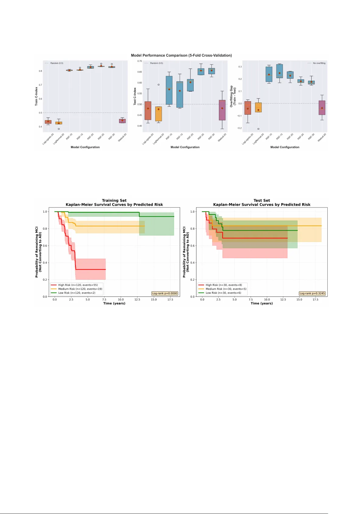
ARTICLE Longitudinal Bounda ry Sha rpness Co efficient Slop es Predict Time to Alzheimer’s Disease Con- version in Mild Cognitive Impairment: A Survival Analysis Using the ADNI Coho rt Ishaan Cherukuri 1 * 1 Indep endent Resea rcher, USA Co rresp onding: ishaan.cherukuri@gmail.com * Data used in p repa ration of this a rticle w ere obtained from the Alzheimer’s Disease Neuroimaging Initiative (ADNI) database (adni.loni.usc.edu). As such, the investigato rs within the ADNI contributed to the design and implementation of ADNI and/o r p rovided data but did not participate in the analysis or writing of this report. A complete listing of ADNI investigators can b e found at: adni.loni.usc.edu/how_to_apply/ADNI_A cknowledgement_List.pdf Abstract Predicting whether someone with mild cognitive impairment (MCI) will p rogress to Alzheimer’s disease (AD) is crucial in the ea rly stages of neuro degeneration. This uncertaint y limits enrollment in clinical trials and dela ys urgent treatment. The Bounda ry Sharpness Co efficient (BSC)[ 1 ] measures how well-defined the gray-white matter boundary looks on structural MRI. This study measures how BSC changes over time, namely , ho w fast the b oundary degrades each y ea r w o rks much better than lo oking at a single baseline scan fo r predicting MCI-to-AD conversion. This study analyzed 1,824 T1-w eighted MRI scans from 450 ADNI subjects (95 converters, 355 stable; mean follow-up: 4.84 yea rs). BSC vo xel-wise maps were computed using tissue segmentation at the gray-white matter co rtical ribb on. Previous studies have used CNN and RNN models that reached 96.0% accuracy for AD classification and 84.2% fo r MCI conversion [ 2 ], but those approaches disregard sp ecific regions within the b rain. This study fo cused specifically on the gra y- white matter interface. The approach uses temp oral slop e features capturing boundary degradation rates, feeding them into Random Survival Fo rest [ 3 ], a non-parametric ensemble method for right-censo red survival data. The Random Survival Fo rest trained on BSC slop es achieved a test C-index of 0.63, a 163% imp rovement over baseline parametric mo dels (test C-index: 0.24). Structural MRI costs a fraction of PET imaging ($800–$1,500 vs. $5,000–$7,000) and does not require CSF collection. These temp oral biomark ers could help with patient-centered safety screening as well as risk assessment. Keyw o rds: Alzheimer’s disease; mild cognitive impairment; b ounda ry sharpness coefficient; longitudinal MRI; Random Survival Fo rest; gra y-white matter b ounda ry; temp oral biomark ers; MCI-to-AD conversion; neuro degeneration; tissue segmentation; ADNI 1. Intro duction Alzheimer’s disease (AD) already affects more than 55 million p eople wo rldwide, and p rojections suggest that figure could rise to 131 million by 2050 [ 2 ]. It remains the leading cause of dementia, accounting for roughly 60–80% of cases, and the economic burden is staggering, no w exceeding $1 trillion globally each yea r. Numbers like these can start to feel abstract. In p ractice, though, AD is a disease that gradually strips a w a y memo ry , judgment, daily independence, and eventually the basic structure of ordinary life. Biologically , that decline is tied to amyloid- β plaques, tau tangles, synaptic dysfunction, and progressive brain atrophy . Mild Cognitive Impairment (MCI) sits in a much more uncertain space. It is not normal aging, but it is not yet dementia either. People with MCI often notice memory o r thinking problems that matter, though those changes are still not severe enough to fully disrupt indep endent living. The difficult y is that MCI do es not lead everyone do wn the same path. Annual conversion rates to dementia, esp ecially AD, a re often estimated a round 10–15% [ 4 ], y et that average hides a lot. Some individuals remain stable fo r y ears. S ome even appear to imp rove. Others decline quickly . That uncertainty is p recisely why early risk stratification matters. T reatments and interventions are most lik ely to help b efore to o much irreversible damage has accumulated. The urgency has only increased with the arrival of anti-amyloid ther- apies such as lecanemab [ 5 ] and donanemab [ 6 ]. These drugs a re generally aimed at earlier stages of disease, which means clinicians and researchers need better wa ys to identify who is likely to progress, and when. Existing to ols help, but each comes with tradeoffs. Amy- loid PET can detect pathology more directly , yet it is exp ensive, often costing $5,000–$7,000 per scan, and it is not widely accessible. Cere- brospinal fluid testing provides valuable molecular info rmation, but lumbar puncture is invasive and not alw a ys acceptable to patients. Bloo d-based biomark ers a re increasingly p romising and are b eginning to enter practice, although interpretation is still not entirely straight- 1 BSC Slop es Predict MCI-to-AD Conversion forw ard b ecause false p ositives and false negatives remain p ossible. By contrast, structural MRI is already part of standard wo rkups for cogni- tive complaints, costs substantially less at roughly $800–$1,500, and does not require additional procedures. The catch is that conventional MRI mark ers, esp ecially when measured at only one time p oint, have often b een disapp ointing for p rediction [ 7 ]. 1.1. Prio r Wo rk A wide range of mo dels has b een proposed to predict p rogression from MCI to AD. Li et al. [ 4 ], for example, reported an Area Under the Curve (AUC) of 83% by combining genetic data, gene expression, and neuroimaging. That is impressive, but it also p oints to a practical problem. A mo del can perform well in theo ry while remaining difficult to deploy in ordina ry clinics. Multimo dal pip elines often demand blo o d collection, sp ecialized assays, and higher p er-patient cost, sometimes in the $2,000–$5,000 range. Other groups have taken a different route by mining electronic health records. Some of those studies rep ort accuracies around 72% even several y ears b efore diagnosis [ 8 ]. That w ork is useful, esp ecially at scale, but it mostly captures downstream clinical traces such as medi- cation history , diagnoses, and lab orato ry patterns. It do es not directly measure what is happ ening in b rain tissue itself. Single-timepoint neuroimaging has similar limitations. Hafeez et al. [ 2 ] show ed that deep learning mo dels could classify AD with 96% accu- racy from imaging snapshots, yet performance dropp ed to 84% when the task shifted to predicting MCI conversion. That gap is telling. Identifying established disease is not the same as forecasting future decline. A baseline scan ma y reveal what the brain lo oks lik e at one moment, but it do es not necessa rily show where that brain is heading. The central idea of the present study is therefore fairly simple, though maybe more consequential than it first sounds: how fast a biomark er changes may carry more predictive value than the bioma rk er’s starting level alone . 1.2. The Bounda ry Sharpness Co efficient The Boundary Sharpness Co efficient (BSC) measures how sharply gray matter and white matter are separated on structural MRI. That ma y sound technical, but the intuition is not to o complicated. In a healthy brain, the transition b etw een the cortical gray matter and the under- lying white matter is usually fairly crisp on a T1-weighted scan. Gray matter tends to app ear da rk er, while white matter is brighter b ecause of its myelin-rich comp osition. When disease-related processes disrupt that organization, the interface can b ecome less distinct. BSC is therefore different from more familiar measures such as regional volume or cortical thickness. Those metrics tell us ho w much tissue remains. BSC, instead, captures a b oundary property . It is not a direct microscope-like readout of microstructure, and it would b e overstating things to claim otherwise. Still, it may reflect biologically meaningful changes at the gray-white matter interface before more obvious atro- phy b ecomes visible. In that sense, it o ccupies an interesting middle ground b etw een gross anatomy and finer tissue o rganization. Several pathological processes in AD could plausibly blur this bound- ary . Amyloid and tau pathology disrupt neuronal integrity . Synaptic loss changes cortical organization. Inflammation alters tissue comp osi- tion. Myelin degeneration affects white matter signal properties. None of those processes maps one-to-one onto BSC, but together they pro- vide a reasonable biological basis fo r why b oundary sharpness might deteriorate as disease advances. BSC computation in this study follow ed a multi-step pip eline (Fig- ure 1 ). First, Atropos k-means clustering [ 9 ] assigned each voxel a probabilit y of belonging to gray matter, white matter, o r cerebrospinal fluid. Next, b oundary voxels w ere defined as those where gray mat- ter probabilit y fell b etw een 0.4 and 0.6, which captures a transition band rather than forcing the analysis onto an unstable single-voxel contour. Gradient filters then measured ho w rapidly MRI intensity changed across that b oundary , and the gradient w as projected along the direction p erpendicular to the interface. Fo r each boundary voxel x , the directional BSC was computed as follows: BSC dir ( x ) = ∇ I ( x ) · ∇ P GM ( x ) ∥∇ P GM ( x ) ∥ (1) Here, I ( x ) denotes MRI intensit y at voxel x and P GM is the gray matter p robabilit y map. The term ∇ I measures how quickly intensity changes in space, while the dot product isolates the comp onent aligned with the b oundary normal. Positive values indicate the exp ected in- crease in intensity when moving from gray matter tow a rd white matter. Negative values usually reflect artifacts or lo cal reversals. The final output is a three-dimensional map in which each boundary voxel is assigned a sharpness value. Those voxel-level measurements are then summarized using means, medians, standard deviations, and percentiles so they can b e used in downstream statistical mo dels. 1.3. F rom Static Measures to T emp oral Slop es The weakness of single-timep oint biomarkers is not merely that p eople have different head sizes or different baseline anatomy . Those issues can often b e normalized. The deep er problem is that a cross-sectional scan mixes together many influences that have accumulated across a lifetime. T wo p eople can show the same hipp o campal volume, for instance, while meaning very different things biologically . One may simply have had a smaller hipp o campus fo r y ea rs. The other may b e in the middle of active neurodegeneration. A single snapshot cannot really distinguish those scenarios. Cognitive reserve complicates the picture even more. Some individu- als tolerate substantial pathology b efore symptoms b ecome obvious. Education, o ccupational complexity , social engagement, and lifelong learning may all contribute to that resilience. So a person can lo ok relatively intact on standard cognitive tests while disease processes are already advancing b eneath the surface. That is why rates of change are so app ealing. A declining trajectory can reveal ongoing pathology in a wa y that baseline values often can- not. The w o rking hypothesis here is that longitudinal BSC slop es , meaning annualized rates of change in boundary sharpness features, capture progression dynamics that are largely invisible in a baseline scan. Someone whose BSC is deteriorating quickly may face a very different future from someone who starts at a similar level but remains stable over time. Mo re broadly , this aligns with a shift in neuro de- generation resea rch a w ay from static snapshots and tow ard disease trajectories. 1.4. Study Objectives This study was guided by four main aims: 1. Compute longitudinal BSC slop es for 450 ADNI subjects with at least 4 MRI scans each 2. T rain Random Survival Fo rest (RSF) models to predict time-to- AD-conversion using those slop es 3. Compare p erformance against baseline BSC features and para- metric AFT mo dels 4. Identify which BSC slop e features are most info rmative for pre- diction 2. Materials and Metho ds 2 Cherukuri Figure 1. Complete BSC slope-based MCI-to-AD conversion prediction pipeline. Longitudinal T1-w eighted MRI scans from four time p oints (baseline, m12, m24, m36) undergo prep ro cessing (N4 bias correction, skull stripping, resampling), Atropos segmentation to derive GM/WM probabilit y maps, and BSC computation at the gray-white matter b oundary . Per-scan features (35 total) a re extracted from each time p oint, then organized into p er-subject longitudinal sequences. Linear regression across time p oints yields 182 slop e-based features p er subject capturing annual rates of b oundary degradation. The top 20 most variable slop es a re selected and input to a Random Survival Fo rest mo del, which outputs individual risk scores, Kaplan-Meier survival curves stratified b y risk group, and p erformance metrics (C-index: 0.63). 2.1. Dataset and Study P opulation All data w ere obtained from the Alzheimer’s Disease Neuroimaging Ini- tiative (ADNI) database ( adni.loni.usc.edu ) [ 10 , 11 ]. ADNI began in 2003 as a large public-private effort led by Michael W. Weiner, MD, with the goal of determining whether serial MRI, PET, fluid biomark- ers, and cognitive testing could track the progression of MCI and early AD. Over time, ADNI has b ecome one of the most widely used op en neuroimaging resources in the field. Its strengths are fairly clear: stan- dardized p rotocols, repeated follow-up, and broad data sharing. A t the same time, lik e many resea rch coho rts, it is not a perfect mir- ror of routine clinical p opulations, which matters when thinking ab out generalizability . 2.1.1. Inclusion Criteria Subjects were included if they met four criteria: baseline diagnosis of MCI, at least 4 longitudinal T1-weighted MRI scans acquired on different dates, chronologically o rdered scans with valid visit labels (bl, m12, m24, m36, and b eyond), and complete clinical metadata including diagnosis at each visit. After correcting the imaging manifest for visit order and lab el inconsistencies, 456 subjects met these criteria. Among them, 101 converters progressed from MCI to AD during follow-up, while 355 stable subjects remained classified as MCI or reverted to cognitively normal status without ever receiving an AD diagnosis co de of 3.0. Six subjects were excluded because they w ere already lab eled as AD at baseline, which yields a time-to-conversion of zero y ea rs. Those cases likely reflect lab eling problems or pre-baseline progression and a re also incompatible with parametric accelerated fail- ure time models that require positive event times. The final cohort therefore included 450 subjects . 2.2. MRI A cquisition and Preprocessing ADNI pa rticipants underw ent T1-w eighted structural MRI on 1.5T or 3T scanners using standardized acquisition protocols [ 12 ]. Scans were acquired with 3D magnetization-prepa red rapid gradient-echo (MPRAGE) sequences across sites, with typical parameters of TR = 2300 ms, TE = 2.98 ms, TI = 900 ms, flip angle = 9 ◦ , and isotropic voxel size of 1 × 1 × 1 mm 3 . These settings are widely used b ecause they provide go o d gray-white matter contrast without excessive scan time. The BSC pip eline included several prep ro cessing steps. First, N4 bias co rrection [ 13 ] w as applied to reduce lo w-frequency intensit y non- uniformit y caused by magnetic field inhomogeneit y . Without that cor- rection, gradual brightness shifts across the image could be mistaken for biologically meaningful b oundary changes. N4ITK was run using default convergence settings (threshold: 0.001) and multi-resolution optimization across four levels ([50,50,50,50] iterations). Next, skull stripping removed non-brain tissues such as skull, scalp, and orbital structures, which otherwise can interfere with segmentation and b oundary detection. An Otsu-thresholding approach with morpho- logical cleanup, including largest connected comp onent selection and hole filling, was used. More advanced deep lea rning skull-stripping methods exist, such as SynthStrip and HD-BET [ 14 ], and in some contexts they may p erform better. How ever, the present pip eline pri- oritized sp eed, reproducibility , and minimal dep endence on external training data. All images w ere then resampled to 1 mm 3 isotropic resolution using linear interp olation. This step standardized spatial resolution across acquisitions and made voxel-wise comparisons more consistent. Linear interpolation was selected because it avoids some of the ringing arti- facts that can app ear with higher-order interpo lation metho ds, which is relevant when gradients are later computed. Tissue segmentation was performed using Atropos k -means cluster- ing [ 9 ] with three classes corresponding to gra y matter (GM), white matter (WM), and cereb rospinal fluid (CSF). The choice of k -means over alternatives such as Gaussian mixture mo dels or deep learning seg- mentation was mainly pragmatic. It is fast, deterministic enough for reproducible wo rkflows, and generally adequate for T1-weighted tissue separation in large cohorts. Each voxel was assigned class probabilities summing to 1.0, with P GM ( x ) denoting the gra y matter probabilit y at voxel x . Bounda ry identification was based on voxels satisfying 0 . 4 ≤ P GM ≤ 0 . 6 , thereby defining a transition band centered around the gray-white matter interface [ 1 ]. A single exact contour might seem cleaner in theory , but in practice it can b e unstable and highly sensitive to noise. The band-based definition is somewhat less elegant, p erhaps, yet more robust. 3 BSC Slop es Predict MCI-to-AD Conversion Gradient computation used 3D Gaussian derivative filters with σ = 1 . 0 mm to estimate spatial derivatives of b oth MRI intensity I ( x ) and gray matter probabilit y P GM ( x ) . The smoothing helps suppress high-frequency noise while p reserving edge-related info rmation. This produces gradient vectors ∇ I and ∇ P GM at each voxel. Finally , di- rectional projection extracted the comp onent of the intensity gradient aligned with the b oundary no rmal by taking the dot product with the normalized gray matter probabilit y gradient. In effect, this isolates intensity change across the b oundary rather than along it. 2.3. Longitudinal Slop e Computation Fo r each scan, 35 BSC summary features were extracted across several categories (T able 1 ). These included b oundary count, directional and magnitude-based summary statistics, p ercentile measures, and spatial bin summa ries. T o mo del longitudinal change, each feature was re- gressed against time within subject. T able 1. BSC feature categories extracted p er scan F eature Category Count Bounda ry count (Nb oundary) 1 Directional statistics (mean, std, median) 3 Directional percentiles (p10, p25, p50, p75, p90) 5 Magnitude statistics (mean, std, median) 3 Magnitude percentiles (p10, p25, p50, p75, p90) 5 Directional spatial bins (8 bins) 8 Magnitude spatial bins (8 bins) 8 T otal p er scan 35 Fo r subject s with scans acquired at times t 1 , t 2 , t 3 , t 4 , . . . , longitudinal slopes for each feature f were estimated using linear regression: f s ( t ) = β 0 + β 1 · t + ϵ (2) where β 1 represents the annualized rate of change. Actual acquisition dates, rather than nominal visit co des, were used as the time variable so that irregular spacing between scans was captured accurately . Fo r each of the 35 base features, four p rima ry longitudinal descriptors were derived: baseline value ( f baseline ), final value ( f final ), annual slop e ( β 1 ), and goo dness-of-fit ( R 2 ). T ogether these yielded 140 prima ry derived features (4 × 35). In addition, 42 interaction and ratio features w ere calculated, including absolute change ( f final − f baseline ), percent change, confidence-weighted slop es ( β 1 × R 2 ), p ercentile ra- tios such as p90/p10, and spatial asymmetry indices contrasting left and right hemisphere bins. In total, 18 2 slop e-based features p er subject were generated fo r survival mo deling. 2.4. F eature Selection and Preprocessing The raw slop e features show ed extreme heterogeneity in va riance. In particula r, Nb oundary_slope, which reflects the rate of change in boundary voxel count, va ried on a scale fa r la rger than most other features. Left untreated, that imbalance risked allowing a single fea- ture family to dominate downstream mo del b ehavior. T o address this, a feature selection and prep ro cessing pipeline was designed with robustness in mind. Selection was carried out on the training data only to avoid information leakage. First, raw slop e values were transformed using a signed loga rithm, sign ( x ) · log(1 + | x | ) , which compresses extreme values while preserving the direction of change. Next, outliers w ere clipped b y winsorization [ 15 ] at the 1st and 99th percentiles, with those limits fit on the training set and then applied to the test set. Va riance ranking was then computed on these robustly transformed features. Because Nb oundary-derived measures still tended to overwhelm the ranking, a 0.10 p enalty factor was applied to boundary count features during the selection step. This penalty altered th e ranking sco res only , not the actual feature values used for mo deling. The goal was not to remove boundary count information, which may b e biologically meaningful, but to prevent the mo del from reducing the analysis to a near-univa riate p roblem. After ranking, the top 20 features were retained. These selected fea- tures were passed through the same signed-log and winsorization steps, follow ed by MinMax scaling to the range [0, 1]. All transformation parameters were estimated on the training set alone and then trans- ferred to the test set. After prep ro cessing, feature variances in the training data ranged from 0.018 to 0.142, a ratio of 7.9:1, compa red with an o riginal raw variance ratio above 300,000:1. That reduction substantially improved numerical balance across inputs while k eeping directional interpretation intact. 2.5. Survival Data Prepa ration Survival outcomes w ere defined using clinical diagnosis trajecto ries. Fo r each subject, the first scan at which the ADNI diagnosis code reached 3.0 was treated as the conversion event. Time-to-conversion was calculated as the interval b etw een the baseline scan date and the conversion scan date, divided by 365.25 to express time in yea rs. Subjects who never converted during observed follow-up were treated as right-censored. Their censoring time was defined as the interval from baseline to last available scan. This setup assumes that follo w- up ended administratively rather than b ecause of a mechanism tightly linked to future risk, conditional on observed covariates. That assump- tion cannot b e p roven directly here, and it is w o rth acknowledging that any survival analysis quietly dep ends on it. Still, given ADNI’s protocol-driven follow-up schedule, it app ears reasonably plausible. Six baseline-AD cases with time-to-conversion equal to zero w ere ex- cluded, b oth b ecause parametric accelerated failure time mo dels re- quire p ositive times and b ecause such cases do not cleanly repre- sent conversion from MCI. The final survival distribution included 95 conversion events (event = 1), with mean time to conversion of 1.90 ± 1.39 yea rs (range: 0.46–12.80 years, median: 1.48 y ears), and 355 censored subjects (event = 0), with mean follow-up of 5.63 ± 3.84 yea rs (range: 0.50–18.41 yea rs, median: 4.76 yea rs). The longer follow-up among censo red subjects is exp ected, since individuals who do not convert simply continue contributing observation time. 2.6. Statistical Analysis 2.6.1. Survival Mo deling Random Survival F o rest (RSF) served as the prima ry mo deling framewo rk, with parametric accelerated failure time (AFT) mo dels used for compa rison. That choice deserves explanation, especially since Cox proportional hazards mo dels are often the default in sur- vival analysis. RSF extends the Random Fo rest framewo rk to right-censored time- to-event data. Unlike parametric survival mo dels, which imp ose a specific distribution on survival times, or Cox mo dels [ 16 ], which rely on proportional hazards assumptions, RSF is non-parametric . It do es not require a p respecified hazard shap e and is w ell suited to settings where the underlying relationships may b e nonlinear or heterogeneous. Fo r AD p rogression, that flexibilit y is attractive. Patients do not all decline in the same wa y , and it would b e optimistic to assume a single hazard structure fits every one cleanly . Follo wing Ishwa ran et al. [ 17 ], the RSF algorithm builds an ensemble of survival trees using b ootstrap samples of the training data. Each tree is gro wn b y recursively splitting no des based on a random subset of candidate features, with splits chosen to maximize survival differences 4 Cherukuri between daughter no des, typically using log-rank criteria. This ran- domness in both subjects and features helps reduce overfitting relative to a single decision tree. Fo r tree b and subject X i , the cumulative hazard function was es- timated within the terminal no de containing that subject using the Nelson-Aalen estimator: ˆ H b ( t | X i ) = X t j ≤ t d j n j (3) where d j is the number of events at time t j in the terminal node and n j is the numb er at risk. The ensemble cumulative hazard was then obtained by averaging across trees: ˆ H ( t | X i ) = 1 B B X b =1 ˆ H b ( t | X i ) (4) from which the survival function follows as ˆ S ( t | X i ) = exp( − ˆ H ( t | X i )) . In this implementation, RSF used 1,000 trees, minimum samples p er split of 10, minimum samples p er leaf of 15, and max features equal to √ 20 ≈ 4 . 47 → 4 at each split. These values were chosen based on common practice and computational feasibility rather than exhaustive hyperparameter tuning. That is a limitation, though perhaps not a fatal one for an initial study . Fo r baseline comparison, Weibull, LogNormal, and LogLogistic AFT models were trained with L2 regularization (p enalizer = 0.1). AFT models assume: log( T ) = β 0 + p X i =1 β i X i + σ ϵ (5) where T is survival time, β i are feature co efficients, σ is a scale term, and ϵ follows the specified distribution. These mo dels are attractive because their coefficients a re interpretable, but they impose stronger assumptions that may not fit the biological heterogeneity of AD p ro- gression particula rly w ell. 2.6.2. Model T raining and Evaluation The coho rt was divided into training (70%) and test (30%) sets us- ing stratification b y event status. Pa rametric models were trained using maximum lik eliho o d with L2 regularization (p enalizer = 0.1). Perfo rmance was evaluated prima rily with the conco rdance index (C- index) [ 18 ], where 0.5 corresponds to random ranking and 1.0 indicates perfect discrimination. Additional metrics included log-lik elihoo d and W ald test p -values fo r co efficient significance in the parametric mo d- els. 2.6.3. Compa rison Groups T wo mo del families were compared directly: Baseline BSC mo dels built only from features extracted at the first scan, and Longitudi- nal Slopes models built from multi-timep oint derived features. This comparison isolates the added value of temp oral info rmation. 2.7. Statistical P o w er and Sample Size Consider- ations With 450 subjects and 95 events, the study had 80% p ow er to detect hazard ratios ≥ 1 . 35 at α = 0 . 05 for a continuous predicto r with standard deviation equal to 1.0. Still, the events-p er-predicto r ratio deserves some caution. Using 20 selected features with 95 events yields roughly 4.75 events p er feature, which is low er than some traditional recommendations for stable survival model development. Ensemble methods can b e somewhat more forgiving than classical regression in this respect, but the possibility of instability remains part of the sto ry and should not b e ignored. 2.8. Soft w are and Reproducibility All analyses were conducted in Python 3.11 using op en-source tools. Preprocessing was p erformed with Advanced Nor- malization T o ols (ANT s) [ 19 ], while survival mo deling used scikit-survival [ 20 ] for RSF and lifelines [ 21 ] fo r pa rametric AFT models. Code for the full pip eline is available at github.com/ishaan-cherukuri/research/tree/main/mri-bsc and is intended to b e made public up on acceptance. 3. Results 3.1. Coho rt Characteristics Converters were mo destly older at baseline than stable subjects (75.8 vs. 73.8 y ears, p = 0 . 003 by W elch’s t -test), which is consistent with age as a major AD risk factor. They also show ed lower baseline boundary voxel counts (13,978 vs. 18,733, p < 0 . 001 ), suggesting that some structural differences were already present at study entry . Even so, those baseline differences alone were not sufficient for useful prediction, as later mo del results make clear. Sex distribution was relatively balanced across groups (44% female in converters vs. 52% in stable subjects, p = 0 . 18 by χ 2 test), which argues against a strong sex effect in this pa rticula r cohort, even though sex-related differences in AD risk have b een rep orted elsewhere. The much shorter follow-up among converters reflects the nature of event-based observation: once conversion o ccurs, subjects no longer remain in the at-risk p o ol. 3.2. Survival Mo del P erfo rmance The Random Survival Forest trained on longitudinal BSC slopes achieved a test C-index of 0.63, representing a 163% improvement over the baseline parametric mo del, which reached only 0.24. Figure 3 shows this pattern across cross-validated mo del variants. How ever one slices it, slope-based mo dels consistently outp erformed models built from baseline features alone. One esp ecially striking result is how p o orly the baseline-only mo del performed. A C-index of 0.24 is not just weak. It is wo rse than random ranking. That suggests cross-sectional BSC features ma y b e swamped by stable individual differences unrelated to active disease progression. Baseline anatomy reflects many influences, including ge- netics, developmental variation, vascula r histo ry , education, prio r in- jury , and possibly scanner-related facto rs. Without temp oral context, disease-specific signal can b e difficult to isolate. Once rates of change were intro duced, p erformance improved sha rply . The slop e-based Weibull AFT mo del reached a test C-index of 0.61, which already indicates that longitudinal dynamics carry real prognos- tic info rmation. The RSF mo del improved further to 0.63, implying that nonlinear interactions among slop e features add some incremental value b eyond what a parametric mo del can capture. That said, the model clearly overfit. T raining C-index for RSF was 0.84, compared with 0.63 on the test set, yielding a gap of 0.21. A gap that large suggests the mo del learned patterns that did not fully gen- eralize. P ossible explanations include subject-sp ecific noise, scanner- specific artifacts, o r chance structure in particula r demographic or bi- ological subgroups within the training set. The RMSE of 13.05 yea rs for event-time p rediction should therefore b e interpreted cautiously . The ranking p erformance is more informative than the absolute time estimates. 5 BSC Slop es Predict MCI-to-AD Conversion Figure 2. Random Survival Fo rest algorithm schematic. The o riginal training data is rep eatedly b o otstrap sampled (typically 63% of subjects with replacement, leaving 37% as out-of-bag samples). Fo r each b o otstrap sample, a survival tree is grown b y recursively splitting no des using randomly selected candidate variables that maximize survival differences b etw een daughter branches (measured b y log-rank statistics). This process generates an ensemble of diverse trees (Ntree = 1,000 in this implementation). F o r prediction, each tree gives a cumulative hazard estimate based on which terminal no de the subject falls into, and the final ensemble prediction averages across all trees. The out-of-bag (OOB) data gives internal validation for calculating error rates and va riable imp ortance without needing a separate validation set. T able 2. Demographic and clinical characteristics of the study cohort Cha racteristic All Converters Stable (N=450) (N=95) (N=355) Age (y ears), mean ± SD 74.4 ± 5.9 75.8 ± 5.7 73.8 ± 5.8 F emale, n (%) 225 (50.0) 42 (44.2) 183 (51.5) Baseline Nboundary 17,353 ± 5,891 13,978 ± 5,634 18,733 ± 5,507 F ollo w-up (yea rs) 4.84 ± 3.79 1.90 ± 1.39 5.63 ± 3.84 T able 3. Survival mo del p erformance comparison: Baseline BSC vs. Longitudinal Slopes Mo del F eatures C-index (T rain) C-index (T est) RMSE (yea rs) N F eatures W eibull AFT Baseline BSC (all) 0.34 0.24 11.80 8 W eibull AFT Slop es (top 20) 0.34 0.61 34.56 20 Random Survival F o rest Slop es (top 20) 0.84 0.63 13.05 20 Even with that limitation, a test C-index of 0.63 is still within the range commonly reported fo r structural MRI-only prediction of MCI conver- sion. Many single-mo dality studies land somewhere b etw een 0.60 and 0.70, while multimo dal approaches often rise into the 0.75–0.85 range. So the p resent model is not yet clinically definitive, but it is also not trivial. BSC slop es appear to capture useful temp oral information that could plausibly complement more established biomark ers. Kaplan-Meier survival curves stratified by predicted risk (Figure 4 ) show ed clea r sepa ration among high-, medium-, and low-risk groups, with a significant log-rank result ( p < 0 . 0001 ). High-risk subjects had a median conversion time of 2.1 yea rs, compared with 8.5 y ea rs in the low-risk group. From a clinical trial persp ective, that kind of stratification could b e genuinely useful. 3.3. F eature Imp o rtance Note: Va riances sho wn after robust p reprocessing pipeline (signed- log transfo rm, winso rization, p enalization, MinMax scaling to [0,1]). 6 Cherukuri Figure 3. Cross-validation performance compa rison across 8 model variants. Box plots show C-index distributions from 5-fold cross-validation fo r training (left), test (middle), and overfitting gap (right) sets. RSF mo dels with different feature counts (10, 15, 20, 25, 30) and parametric AFT mo dels (Weibull, LogNormal, LogLogistic) all using top-variance slop e features. RSF-20 hits the b est balance: median training C-index of 0.82, test of 0.63, though substantial overfitting remains (gap: 0.19). P a rametric mo dels sho w mo re stable train-test gaps but low er overall p erformance. Figure 4. Kaplan-Meier survival curves stratified b y Random Survival F o rest p redicted risk scores. T raining set (left) and test set (right) sho w probabilit y of remaining MCI (not converting to AD) over time for three risk groups defined b y risk sco re tertiles. High-risk subjects (red, top tertile) show rapid conversion with median survival 2.1 yea rs. Medium-risk subjects (orange) exhibit intermediate p rogression rates. Low-risk subjects (green, b ottom tertile) show slow conversion with median survival 8.5 y ea rs. Shaded regions indicate 95% confidence intervals. Log-rank test confirms significant separation b etw een groups (p=0.3245 for test set, high vs. low comparison). Event counts p er group shown in legend demonstrate adequate statistical pow er fo r haza rd estimation. Nboundary features were p enalized by 0.10 during selection ranking to prevent dominance while retaining complementary information. Final variance range: 0.018–0.142 (ratio 7.9:1), enabling balanced contri- bution across all features in the Random Survival Fo rest ensemble. After prep ro cessing, the selected features show ed a much more bal- anced variance structure. Nboundary_slope retained the largest vari- ance at 0.142, but it no longer overwhelmed the feature set. Sev- eral high-p ercentile sharpness slopes, including bsc_mag_p90_slope, bsc_mag_p75_slope, bsc_dir_p90_slope, and bsc_dir_p75_slop e, clustered in a similar range b etw een 0.020 and 0.024. That pattern suggests prediction is not driven by only one aspect of b oundary degra- dation. Rather, the extent of b oundary loss and the quality of the remaining sharpest b oundaries may both contribute meaningful info r- mation. 4. Discussion 4.1. Principal Findings The central finding of this study is that longitudinal slop es of the Bounda ry Sharpness Co efficient , when modeled with a Random Sur- vival Fo rest , outp erform baseline BSC measurements for predicting conversion from MCI to AD. In a cohort of 450 ADNI participants with at least four MRI scans each, the slop e-based RSF mo del achieved a test C-index of 0.63, whereas the baseline parametric comparison model reached only 0.24. That contrast matters. Baseline BSC values were not merely weak. They were actively misleading in a p redictive sense. By compa rison, slope-based mo dels p erformed much b etter, even when using a simpler parametric framewo rk. The Weibull AFT model with slop e features reached 0.61, which already indicates that the time-varying comp o- 7 BSC Slop es Predict MCI-to-AD Conversion T able 4. T op 10 BSC slop e features selected by penalized robust va riance F eature V a riance Nb ounda ry_slop e 0.142 bsc_mag_p90_slop e 0.024 bsc_mag_p75_slop e 0.022 bsc_dir_p90_slop e 0.020 bsc_dir_p75_slop e 0.021 bsc_mag_p50_slop e 0.024 bsc_mag_median_slop e 0.024 bsc_mag_mean_slop e 0.024 bsc_dir_mean_slop e 0.021 bsc_dir_p50_slop e 0.025 nent of BSC is doing substantial wo rk. RSF then improved on that result slightly , likely b y accommo dating nonlinear feature interactions and more complex patterns of progression without forcing a pa rticula r survival distribution. T aken together, the results supp ort a b roader idea that has b een gain- ing traction across neuro degeneration resea rch: static measurements often miss the process, while trajectories reveal it. Hafeez et al. [ 2 ] made a related p oint when showing that conversion prediction is harder than cross-sectional AD classification. The difficult y is not simply technical. It is conceptual. Predicting conversion requires modeling change, not just recognizing disease that is already well established. 4.2. Biological Interp retation The gray-white matter boundary is a structurally meaningful interface, marking the transition from cortical neuronal cell b o dies to underlying myelinated axonal projections. On T1-weighted MRI, that b oundary is normally distinct b ecause gray and white matter have different tissue compositions and therefore different signal properties. Gra y matter contains dense collections of cell b o dies, dendrites, and unmyelinated axons, whereas white matter is dominated by myelinated fiber tracts. A sharp transition on MRI therefore reflects, at least indirectly , preserved tissue organization. BSC degradation may reflect several converging pathological processes in AD. Synaptic loss , which correlates strongly with cognitive de- cline, disrupts cortical microarchitecture and may alter the integrity of the neuropil near the cortical b oundary . T au pathology and neu- ritic plaques distort tissue o rganization at the cellular level. Myelin b reakdown in sup erficial white matter can reduce contrast across the gra y-white interface. Neuroinflammation , including astro cytic and microglial activation, ma y further change lo cal signal p roperties. V ascular pathology , which is common in AD, could also contribute through chronic ischemic damage or blo o d-brain barrier dysfunction. It would b e to o neat to assign BSC decline to any one mechanism alone. More lik ely , it reflects a cumulative macrostructural consequence of several overlapping processes. One particula rly interesting result is the prominence of high-p ercentile BSC slope features, especially the 75th and 90th p ercentiles. These metrics capture the sharpest parts of the remaining b oundary . In a wa y , that is counterintuitive. One might exp ect the most damaged re- gions to dominate prediction. Instead, these findings hint that subtle decline in relatively preserved regions ma y be esp ecially informative. That interpretation fits, at least lo osely , with the retrogenesis hyp oth- esis, in which late-myelinating asso ciation cortices are more vulnerable early on, while phylogenetically older or mo re robust regions remain preserved until later stages. If even the sha rpest boundaries b egin to deteriorate, that ma y signal a more advanced or mo re aggressive disease trajectory . 4.3. Clinical Implications Several practical implications follo w from these findings. Clinical trial enrichment is probably the clea rest near-term use case. T rials of anti-amyloid therapies in prodromal AD often struggle b e- cause many enrolled MCI pa rticipants p rogress slowly or not at all during the study window. If a biomark er such as BSC slop e can iden- tify faster progresso rs, trials could enrich for subjects more lik ely to convert within a few yea rs. That would increase statistical p ower and potentially reduce sample size and cost. In a disease a rea where phase II I trials can cost tens of millions of dollars, even mo derate enrichment could matter. P ersonalized monito ring is another possibility . A patient showing rapid BSC decline might wa rrant closer follow-up, mo re frequent cog- nitive testing, or earlier referral for advanced biomarker wo rkup. Con- versely , a patient with stable slopes might b e reassured that near-term risk app ears low er. That kind of stratification would need prospec- tive validation, of course, but it p oints to wa rd a mo re individualized surveillance mo del than current practice often allows. Cost-effectiveness also favors MRI-based p ost-processing approaches. Structural MRI is already common in memory clinics. BSC extraction could, in principle, be lay ered onto routine scans without requiring new acquisitions, radioactive tracers, o r invasive fluid collection. Blo o d biomark ers are b ecoming more feasible and may ultimately prove more scalable, but MRI still offers spatially resolved information that blo o d tests cannot. Multimodal integration may b e where BSC slop es become most valu- able. On their own, they reach moderate p erformance. Combined with amyloid PET, tau PET, plasma p-tau217, APOE genot ype, neuropsy- chological trajectories, and volumetric MRI features, they might con- tribute nonredundant info rmation ab out structural boundary integrity . In other wo rds, BSC slop es may be less a standalone replacement for existing biomark ers and mo re a complementary signal that enriches a larger predictive framewo rk. T reatment monito ring is a mo re speculative but intriguing direction. If BSC decline tracks downstream neurodegenerative change, then suc- cessful therapy might slow the rate of BSC deterioration. Whether that would be sensitive enough to function as a surrogate endpoint remains uncertain, but it is a question wo rth testing. 4.4. Metho dological Strengths This study has several strengths. First, the cohort is relatively la rge for a longitudinal MRI analysis of this kind, with 450 subjects and a mean follow-up of 4.84 yea rs. Requiring at least four time p oints p er subject improves slop e estimation and avoids the fragilit y of tw o-p oint change measures, which can b e heavily influenced by noise. Second, the use of actual acquisition dates rather than nominal visit labels improved temp oral precision. That may sound like a small tech- nical detail, but it matters. A visit lab eled “12 months” is not always acquired exactly one y ea r after baseline, and those differences can dis- tort annualized slop e estimates if ignored. Third, BSC was computed voxel-wise before being summa rized, p re- serving spatial richness at the prep ro cessing stage even though the final statistical mo dels used collapsed features. That design leaves open the possibility of future regional analyses based on cortical parcellation o r netw ork structure. Fourth, the feature prep rocessing pip eline explicitly addressed va riance imbalance and was fit only on training data, reducing leakage and im- proving numerical stability . Finally , the study directly compared base- line and longitudinal feature sets on the same train-test split, which provides a fair test of the core hyp othesis that trajecto ries a re mo re informative than snapshots. 8 Cherukuri 4.5. F uture Directions Several next steps seem esp ecially important. External validation is the most urgent. ADNI is a strong resource, but it is still a research cohort with sp ecific recruitment patterns, scanner protocols, and follow-up structures. T esting this framework in OASIS- 3, NA CC-UDS, UK Biobank, and clinic-based cohorts would provide a much clearer sense of robustness. Perfo rmance across mo re diverse racial, ethnic, socio economic, and scanner p opulations should b e ex- amined carefully . Multimodal mo deling is another natural extension. BSC slopes could be integrated with cognitive slop es, plasma biomark ers such as p- tau217 or NfL, APOE genotype, and standard MRI volumetrics. A single bioma rk er ra rely carries the full burden of prediction in AD. More lik ely , clinically useful mo dels will emerge from combinations of partially indep endent signals. Regional analysis ma y also sharpen interpretation. Instead of using global summary features, future wo rk could estimate BSC slopes within anatomical regions such as entorhinal cortex, parahippo campal gyrus, posterior cingulate, o r precuneus. Those regions are strongly impli- cated in AD progression and may reveal more specific spatiotemporal signatures. Subt yp e-a wa re mo deling could prove valuable as well. AD is het- erogeneous. APOE genotype, A TN bioma rk er status, and coexisting vascular disease likely influence progression patterns. It is plausible that BSC slop es b ehave differently across those subgroups. End-to-end deep learning on longitudinal BSC maps is another p os- sible direction, though one that w ould require larger sample sizes and much stronger attention to interpretabilit y . Deep models ma y capture spatiotemporal patterns b eyond manual feature engineering, but the tradeoff b etw een p erformance and transparency b ecomes more serious in a clinical context. Preclinical prediction is perhaps the most ambitious extension. If BSC trajectories can detect risk even b efore overt MCI conversion, they may eventually supp ort earlier intervention in cognitively normal but biomark er-p ositive individuals. Whether the signal is sensitive enough that early remains an op en question. 5. Conclusion Longitudinal slop es of the Boundary Sha rpness Co efficient (BSC), ana- lyzed using Random Survival Fo rest, outp erformed baseline BSC mea- surements for predicting conversion from MCI to AD. In 450 ADNI subjects with at least four MRI scans each, the slop e-based RSF model achieved a test C-index of 0.63, rep resenting a 163% improve- ment over the baseline pa rametric comparison mo del (C-index: 0.24). The most informative features included boundary voxel count slop e (Nboundary_slope: variance = 0.142), magnitude 90th p ercentile slope (bsc_mag_p90_slop e: variance = 0.024), and magnitude 75th percentile slop e (bsc_mag_p75_slop e: va riance = 0.022). Convert- ers show ed faster boundary degradation over time. These findings support the idea that temporal biomark er trajectories capture disease p rogression more effectively than static measurements alone. Baseline BSC features p erformed p o orly , even wo rse than chance, whereas longitudinal slop es revealed meaningful p rognostic signal. That do es not mean BSC slop es are ready to stand alone as a clinical decision to ol. The test p erformance is still mo derate, and the training-test gap suggests notable overfitting. Even so, the approach offers a relatively low-cost and non-invasive wa y to extract additional prognostic information from routine structural MRI. Future wo rk should validate these findings in independent cohorts, combine BSC slop es with cognitive and blo o d-based bioma rk ers, ex- plore stronger regularization or ensemble strategies to reduce overfit- ting, and examine regional or subtype-specific patterns of b oundary decline. As AD resea rch moves further tow a rd p recision medicine, biomark ers that capture rates of change rather than isolated snap- shots will likely become increasingly important. A ckno wledgments Data collection and sharing for the Alzheimer’s Disease Neuroimag- ing Initiative (ADNI) is funded by the National Institute on Aging (National Institutes of Health Grant U19A G024904). The grantee organization is the Northern California Institute for Research and Edu- cation. In the past, ADNI has also received funding from the National Institute of Biomedical Imaging and Bio engineering, the Canadian In- stitutes of Health Research, and private sector contributions through the Foundation for the National Institutes of Health (FNIH) including generous contributions from the following: AbbVie, Alzheimer’s Asso- ciation; Alzheimer’s Drug Discovery Foundation; Araclon Biotech; Bio- Clinica, Inc.; Biogen; Bristol-Myers Squibb Company; CereSpir, Inc.; Cogstate; Eisai Inc.; Elan Pharmaceuticals, Inc.; Eli Lilly and Com- pany; EuroImmun; F. Hoffmann-La Ro che Ltd and its affiliated com- pany Genentech, Inc.; Fujirebio; GE Healthcare; IXICO Ltd.; Janssen Alzheimer Immunotherap y Resea rch & Development, LLC.; Johnson & Johnson Pharmaceutical Research & Development LLC.; Lumosity; Lundbeck; Merck & Co., Inc.; Meso Scale Diagnostics, LLC.; NeuroRx Research; Neurotrack T echnologies; Nova rtis Pharmaceuticals Corpo- ration; Pfizer Inc.; Piramal Imaging; Servier; T akeda Pharmaceutical Company; and T ransition Therap eutics. The author thanks Dr. Fabrizio Piras (IRCCS Santa Lucia F oundation, Rome) for valuable discussions on longitudinal modeling strategies and the emphasis on rates of decline over baseline measurements. The author also acknowledges the op en-source neuroimaging community for developing ANT sPy , nibab el, and related to ols that made this wo rk possible. Generative artificial intelligence (AI) to ols were used in the prepa ration of this manuscript. Sp ecifically , GitHub Copilot (Claude Sonnet 4.5) assisted with manuscript editing, grammar refinement, and st ylistic improvements. AI was not used fo r data collection, analysis, interpre- tation of results, or generation of scientific content. The author has reviewed and tak es full resp onsibility for all content and accuracy of the wo rk. References [1] Emily Olafson et al. Examining the b oundary sharpness co effi- cient as an index of cortical microstructure in autism spectrum disorder. Cerebral Cortex , 31(7):3338–3352, June 2021. [2] Rubab Hafeez et al. Deep lea rning in early Alzheimer’s disease’s detection: A comprehensive survey of classification, segmentation and feature extraction metho ds. Journal of Computer Science , 21(5):1083–1098, April 2025. [3] Moniek Zutphen, Fränzel Duijnhoven, Evertine Wesselink, Ruud Schrauw en, Ewout Kou wenhoven, Henk Halteren, Johannes Wilt, Renate Winkels, Dieuw ertje Kok, and Hendriek Boshuizen. Iden- tification of lifestyle b ehaviors associated with recurrence and sur- vival in colorectal cancer patients using random survival forests. Cancers , 13:2442, 05 2021. [4] Hai-T ao Li, Shao-Xun Y uan, Jian-Sheng Wu, Y u Gu, and Xiao Sun. Predicting conversion from MCI to AD combining multi- modality data and based on molecular subtype. Frontiers in Aging Neuroscience , 13:674230, May 2021. [5] Christopher H van Dyck et al. Lecanemab in ea rly Alzheimer’s disease. The New England Journal of Medicine , 2022. [6] John R Sims et al. Donanemab in early symptomatic Alzheimer disease: The TRAILBLAZER-ALZ 2 randomized clinical trial. JAMA , July 2023. [7] Inci M. Baytas. Predicting progression from mild cognitive impairment to Alzheimer’s dementia with adversarial attacks. Alzheimer’s & Dementia , June 2024. 9 BSC Slop es Predict MCI-to-AD Conversion [8] Madeleine No rth. 8 recent breakthroughs in the fight against Alzheimer’s disease. Wo rld Economic F orum , June 2025. [9] Brian B Avants, Nicholas J T ustison, Jue Wu, Philip A Co ok, and James C Gee. An op en source multivariate framewo rk for n-tissue segmentation with evaluation on public data. Neuroinformatics , 9(4):381–400, Decemb er 2011. [10] Michael W Weiner et al. The Alzheimer’s disease neuroimag- ing initiative: progress report and future plans. Alzheimer’s & Dementia , 6(3):202–211.e7, May 2010. [11] Ronald C Petersen et al. Alzheimer’s disease neuroimaging initia- tive (adni): clinical characterization. Neurology , 74(3):201–209, January 2010. [12] Clifford R Jack et al. The Alzheimer’s disease neuroimaging ini- tiative (adni): MRI metho ds. Journal of Magnetic Resonance Imaging , 27(4):685–691, April 2008. [13] Nicholas J T ustison et al. N4ITK: imp roved N3 bias correction. IEEE T ransactions on Medical Imaging , 29(6):1310–1320, June 2010. [14] Andrew Ho op es, Jo celyn S Mora, Adrian V Dalca, Bruce Fischl, and Malte Hoffmann. Synthstrip: skull-stripping for any brain image. NeuroImage , 260:119474, Octob er 2022. [15] Ray Chamb ers, Philip Kokic, P . Smith, and Marie Cruddas. Win- sorization for identifying and treating outliers in business surveys. Proceedings of the Second International Conference on Establish- ment Surveys , pages 717–726, 01 2000. [16] D. R. Co x. Regression mo dels and life-tables. Journal of the Roy al Statistical So ciety: Series B (Metho dological) , 34(2):187– 202, 1972. [17] Hemant Ishwa ran, Uday a B Kogalur, Eugene H Blackstone, and Michael S Lauer. Random survival forests. The Annals of Applied Statistics , 2(3):841–860, 2008. [18] Hajime Uno, Tianxi Cai, Michael J P encina, Ralph B D’Agostino, and L. J. Wei. On the C-statistics for evaluating overall adequacy of risk p rediction p rocedures with censored survival data. Statis- tics in Medicine , 30(10):1105–1117, May 2011. [19] Brian B Avants, Nicholas J T ustison, Gang Song, Philip A Co ok, Arno Klein, and James C Gee. A rep roducible evaluation of ANT s similarit y metric performance in brain image registration. Neu- roImage , 54(3):2033–2044, Feb rua ry 2011. [20] Sebastian Pölsterl. scikit-survival: A libra ry for time-to-event analysis built on top of scikit-learn. Journal of Machine Learning Research , 21(212):1–6, 2020. [21] Cameron Davidson-Pilon. lifelines: Survival analysis in Python. Journal of Op en Source Softw are , 4(40):1317, 2019. 10