Calorimeter Shower Superresolution with Conditional Normalizing Flows: Implementation and Statistical Evaluation

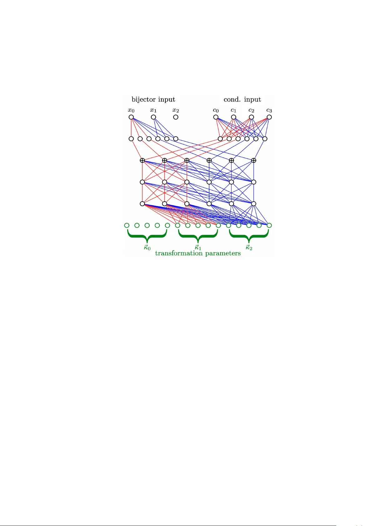
Universit à degli Studi di Geno v a Scuola di Scienze Ma tema tiche, Fisiche e Na turali La urea Magistrale in Fisica Calo rimeter Sho w er Sup erresolution with Conditional no rmalizing Flo ws: Implementation and Statistical Evaluation Candidato Andrea Cosso Relatori Dott. Riccardo T orre Dott. Marco Letizia Correlatore Dott. Andrea Co ccaro Anno a ccademico 2024/2025 Contents Abstract . . . . . . . . . . . . . . . . . . . . . . . . . . . . . . . . . . . vi In tro duction 1 1 Mac hine Learning Essen tials 6 1.1 Mac hine Learning in Ph ysics . . . . . . . . . . . . . . . . . . . . . 6 1.1.1 The three paradigms of mac hine learning . . . . . . . . . . 6 1.1.2 Data discussion . . . . . . . . . . . . . . . . . . . . . . . . 8 1.1.3 Statistical learning . . . . . . . . . . . . . . . . . . . . . . 9 1.1.3.1 The Loss function . . . . . . . . . . . . . . . . . 9 1.1.3.2 An introduction to the statistical mo del . . . . . 11 1.2 In tro duction to neural net works . . . . . . . . . . . . . . . . . . . 22 1.2.1 P erceptron . . . . . . . . . . . . . . . . . . . . . . . . . . . 22 1.2.2 Multi-la yer p erceptron . . . . . . . . . . . . . . . . . . . . 24 2 F rom Generation to V alidation: Principles and Ev aluation Met- rics 26 2.1 Generativ e mo dels in ph ysics . . . . . . . . . . . . . . . . . . . . . 26 2.2 Normalizing Flows: F ormalism and Overview . . . . . . . . . . . . 33 2.2.1 The core idea . . . . . . . . . . . . . . . . . . . . . . . . . 33 2.2.2 The formalism of normalizing Flo ws . . . . . . . . . . . . . 33 2.2.3 Coupling and A utoregressive ﬂo ws . . . . . . . . . . . . . . 36 2.3 Mask ed A utoregressive Flo w (MAF) . . . . . . . . . . . . . . . . . 39 2.3.1 MADE: Masked A uto enco der for Distribution Estimation . 41 2.3.2 Rational Quadratic Spline (RQS) . . . . . . . . . . . . . . 45 2.4 Ev aluating Generativ e Mo dels . . . . . . . . . . . . . . . . . . . . 47 2.4.1 T w o-sample h yp othesis testing . . . . . . . . . . . . . . . . 49 2.4.2 T est statistics . . . . . . . . . . . . . . . . . . . . . . . . . 51 ii 2.4.2.1 Sliced W asserstein distance . . . . . . . . . . . . 51 2.4.2.2 K olmogorov-Smirno v (KS) inspired test statistics 52 2.4.2.3 Maxim um Mean Discrepancy (MMD) . . . . . . 54 2.4.2.4 F réc het Gaussian Distance (F GD) . . . . . . . . . 55 2.4.2.5 Lik eliho o d-ratio . . . . . . . . . . . . . . . . . . . 55 3 Calorimeter Ph ysics and Detector Principles 57 3.1 Electromagnetic calorimetry . . . . . . . . . . . . . . . . . . . . . 60 3.1.1 In teraction with matter . . . . . . . . . . . . . . . . . . . . 60 3.1.2 Electron-Photon cascades . . . . . . . . . . . . . . . . . . 60 3.1.3 Homogeneous calorimeters . . . . . . . . . . . . . . . . . . 63 3.1.4 Sampling calorimeters . . . . . . . . . . . . . . . . . . . . 63 3.2 Hadron calorimetry . . . . . . . . . . . . . . . . . . . . . . . . . . 63 3.2.1 Hadronic show ers . . . . . . . . . . . . . . . . . . . . . . . 64 3.3 Limitations . . . . . . . . . . . . . . . . . . . . . . . . . . . . . . 64 3.4 Calorimeter sup erresolution . . . . . . . . . . . . . . . . . . . . . 66 4 Implemen tation and Exp erimen tal Setup 68 4.1 Dataset Description . . . . . . . . . . . . . . . . . . . . . . . . . . 68 4.1.1 The dataset . . . . . . . . . . . . . . . . . . . . . . . . . . 68 4.2 Building the datasets . . . . . . . . . . . . . . . . . . . . . . . . . 70 4.2.1 The vo xelization . . . . . . . . . . . . . . . . . . . . . . . 70 4.2.2 Conditional inputs . . . . . . . . . . . . . . . . . . . . . . 72 4.2.3 Prepro cessing steps . . . . . . . . . . . . . . . . . . . . . . 73 4.3 Arc hitecture . . . . . . . . . . . . . . . . . . . . . . . . . . . . . . 74 4.4 T raining Strategy . . . . . . . . . . . . . . . . . . . . . . . . . . . 78 4.4.1 Hardw are and Softw are Environmen t . . . . . . . . . . . . 78 4.4.2 Loss F unction . . . . . . . . . . . . . . . . . . . . . . . . . 80 4.4.3 Optimizer and Learning Rate Sc hedule . . . . . . . . . . . 80 4.5 Ev aluation . . . . . . . . . . . . . . . . . . . . . . . . . . . . . . . 81 4.6 Results . . . . . . . . . . . . . . . . . . . . . . . . . . . . . . . . . 88 4.6.1 T raining results . . . . . . . . . . . . . . . . . . . . . . . . 88 4.6.2 Qualitativ e comparison of generated and reference show ers 90 4.6.3 Statistical ev aluation . . . . . . . . . . . . . . . . . . . . . 91 4.6.3.1 Results at full dimensionality . . . . . . . . . . . 92 4.6.3.2 Ph ysically inspired observ ables . . . . . . . . . . 97 iii 5 Lessons Learned and What Comes Next 100 5.1 Summary of Findings . . . . . . . . . . . . . . . . . . . . . . . . . 100 5.2 Ph ysics Implications . . . . . . . . . . . . . . . . . . . . . . . . . 102 5.3 Limitations . . . . . . . . . . . . . . . . . . . . . . . . . . . . . . 103 5.4 Outlo ok and F uture W ork . . . . . . . . . . . . . . . . . . . . . . 104 A ckno wledgemen ts . . . . . . . . . . . . . . . . . . . . . . . . . . . . . 107 A More on Loss F unctions 109 B Second order optimizer: The Newton-Raphson metho d 112 C Use of AI-assisted to ols 114 iv Abstract In High Energy Ph ysics, detailed calorimeter sim ulations and reconstructions are essen tial for accurate energy measuremen ts and particle identiﬁcation, but their high gran ularity mak es them computationally exp ensive. Dev eloping data-driven tec hniques capable of recov ering ﬁne-grained information from coarser readouts, a task kno wn as calorimeter sup erresolution, oﬀers a promising w a y to reduce b oth computational and hardware costs while preserving detector p erformance. This thesis in vestigates whether a generativ e mo del originally designed for fast sim ulation can b e eﬀectiv ely applied to calorimeter sup erresolution. Sp eciﬁcally , the model prop osed in Ref. [1] is re-implemen ted independently and trained on the CaloChallenge 2022 dataset based on the Gean t4 Par04 calorimeter geometry . Finally , the mo del’s performance is assessed through a rigorous statistical ev aluation framew ork, following the metho dology introduced in Ref. [2], to quan- titativ ely test its abilit y to repro duce the reference distributions. vi Intro duction In High Energy Physics (HEP), the Large Hadron Collider (LHC) plays a cen tral role in testing the predictions of the Standard Mo del and exploring p ossible signs of new physics. Bridging theoretical predictions and exp erimental observ ations requires highly detailed simulations grounded in ﬁrst-principles physics. In this con text, HEP relies extensiv ely on sim ulations, follo wing a complex pip eline that encompasses even t generation, detector sim ulation, and reconstruction. Detector in teractions are typically mo deled with high-precision Mon te Carlo tec hniques, most notably implemen ted in Geant4 [3]. Because the accuracy of man y LHC measuremen ts dep ends on suc h sim ulations, the increased data volume an tici- pated in future runs will signiﬁcantly raise the demand for syn thetic even ts and, consequen tly , for computational resources. This gro wing need is exp ected to b e- come a ma jor computational bottleneck in the near future [4–6]. Indeed, the High Luminosity LHC (HL-LHC), whic h will commence op eration in 2030, will increase the luminosit y by a factor of 10, from an in tegrated luminosity of appro ximately ≃ 300 fb − 1 (in Run 3) to L ≃ 3000 fb − 1 [7], dramatically increasing the need for computational resources (see Figure 1). A ma jor part of the computational p ow er go es in to the detector response simulation, particularly that of the calorimeter. In fact, calorimeters are esp ecially computationally demanding due to the high n umber of secondary particles that must b e trac ked and simulated. Therefore, in recent years, with the dev elopmen t of adv anced machine learning techniques, there has b een a gro wing in terest in developing faster calorimeter sim ulations. A t presen t, most fast calorimeter simulations are based on parametrized calorimeter resp onses, th us b ypassing the computationally heavy Geant4 simulations. The problem with these algorithms is that they lac k the ﬁdelity needed to meet the precision requirements of HEP measurements [8–10]. F or this reason, there is a strong global eﬀort to develop new generativ e models capable of addressing the curren t and future c hallenges of detector sim ulation [11]. 1 Intro duction 2 Eﬃcien t sup er-resolution metho ds can oﬀer an alternativ e path: instead of p erforming full ﬁne-granularit y simulations, one can simulate at a coarser dis- cretization and then “upsample” to ﬁne resolution using learned mo dels. This reduces simulation cost, memory usage, and data v olume while reco vering (or appro ximating) the physics ﬁdelit y of ﬁne segmen tation. Preserving ﬁne-grained detector information is essen tial for the accurate re- construction and iden tiﬁcation of particles from detector signatures, which form the basis of all ph ysics analyses. T o illustrate the imp ortance of calorimeter gran ularity , we can consider an example in tro duced in Ref. [12], inv olving single high-energy photons at the LHC, of great interest for precision measurements in Quantum Chromodynamics (QCD) and Electro weak theory [13]. At hadron colliders, the main background source for photons is the electromagnetic decay of high-energy mesons, most frequently π 0 → γ γ , since neutral pions are com- monly pro duced in hadronic in teractions. The signature of such decays at high- energy is often measured as a “fak e single photon” due to the large Loren tz b o ost, whic h results in a small separation b et ween the tw o photons. Resolving the tw o distinct signals from the decay of a single meson requires high spatial resolu- tion, ac hieved b y increasing the calorimeter segmen tation. This is not alwa ys p ossible, since increasing granularit y en tails signiﬁcan t tec hnical and ﬁnancial c hallenges. Indeed, high-gran ularity (HG) directly translates into more readout c hannels, more electronics, higher data rates, increased co oling and p o wer re- quiremen ts, more material, and greater calibration eﬀort, thus making the costs of HG calorimeters prohibitive [14]. Beyond this example, man y physics anal- yses rely on subtle features of calorimeter show ers, such as energy fractions in la yers, cluster substructure, the identiﬁcation of o v erlapping sho w ers, and similar observ ables [12]. Therefore, sup er-resolution can oﬀer a solution b y virtual ly in- creasing the calorimeter resolution without physically adding c hannels, leading to b etter p erformance in ph ysics tasks such as impro ved particle iden tiﬁcation (ID), more accurate reconstruction of ob jects (photons, π 0 , jets), enhanced energy and p osition resolution, and reduced systematic uncertainties. Another important application of sup er-resolution arises in the con text of aging calorimeters. In real exp eriments, detectors inevitably age, front-end elec- tronics degrade, calibrations drift, and gran ularit y may eﬀectiv ely degrade. With time and radiation, cells may fail (dead channels) or b e disabled due to high lev els of noise or false hits that contaminate the measuremen ts [15–17]. In this context, Intro duction 3 a sup er-resolution mo del trained to reconstruct ﬁne-grained sho w er structures from coarse or incomplete data could, in principle, b e used to ﬁll in or recov er the missing energy pattern in dead or disabled regions. Suc h an approac h would oﬀer signiﬁcant beneﬁts, including the reco v ery of otherwise lost information, mitigation of p erformance degradation in aging detectors, and the con tinued use of partially degraded calorimeter sections without ma jor recalibration or replace- men t. Finally , lo oking ahead to the High-Luminosit y LHC (HL-LHC), pile-up may b ecome a critical issue [18]. In a proton–proton collider like the LHC, protons are group ed in bunc hes containing roughly 10 11 protons each. These bunc hes cross each other ev ery 25 ns at the interaction p oin ts (A TLAS, CMS, etc.). Each time t wo bunches cross, more than one proton–proton in teraction can o ccur. All these interactions o ccur within the same detector readout windo w, causing their signals to o verlap. This phenomenon, known as pile-up, refers to the o v erlap of signals from multiple interactions o ccurring in the same or neighboring bunc h crossings. During R un 2 at the LHC, the av erage pile-up w as appro ximately 32 [19, 20], while for Run 3 the v alue was appro ximately 60 [21]. A t the HL- LHC, the av erage num b er of interactions p er bunc h crossing is exp ected to reach 140 to 200 [18], greatly increasing reconstruction complexit y . Sup er-resolution, b y virtual ly increasing the calorimeter resolution, can b ecome a p ow erful to ol to impro ve reconstruction p erformance. In this thesis, w e indep endently replicate the generative mo del in tro duced in Ref. [1] in resp onse to the F ast Calorimeter Simulation Chal lenge (CaloChal- lenge) initiated in 2022 [11], a comm unity challenge for fast calorimetry simula- tion. P articipants were task ed with training their preferred generativ e mo dels on the pro vided calorimeter show er datasets, with the goal of accelerating and ex- panding the dev elopmen t of fast calorimeter sim ulations, while providing common b enc hmarks and a shared ev aluation pip eline for fair comparison. The idea explored in Ref. [1] was to use auxiliary mo dels to generate a coarse represen tation of a calorimeter sho w er and implement a super-resolution algo- rithm to upsample the sho w ers to their ﬁne-grained represen tation. In this con- text, our goal is to replicate only the ﬁnal upsampling mo del, implemen ted as a Normalizing Flow [22, 23] using R ational Quadr atic Spline transformations [24]. The mo del has b een trained on the dataset pro vided by the CaloChal lenge , sp ecif- ically on Dataset 2 , whic h w as generated with the Par04 example of Geant4 . Intro duction 4 The model is then ev aluated follo wing the metho dology in tro duced in Ref. [2]. In the scientiﬁc domain, where high levels of precision and accuracy are required, v alidation presents critical c hallenges. Many existing v alidation metho ds lac k a rigorous statistical foundation, making it diﬃcult to provide robust and reli- able ev aluations. The high precision required in HEP , where accurate mo deling of features, correlations, and higher-order momen ts is essen tial, demands robust p erformance assessment of generative mo dels. T wo-sample h yp othesis testing pro vides a natural statistical framework for p erformance ev aluation. Reference [2] prop oses a robust metho dology for ev aluating tw o-sample tests, fo cusing on non-parametric tests based on univ ariate in tegral probabilit y measures (IPMs). The approach extends 1D-based tests, suc h as the Kolmogoro v–Smirno v [25, 26] or W asserstein distance [27, 28], to higher dimensions by a v eraging or slicing (i.e. pro jecting data onto random directions on the unit sphere). The recen tly pro- p osed unbiased F réchet Gaussian Distance (F GD) [29, 30] and Maximum Mean Discrepancy (MMD) [31, 32] are also included. Reference [2] addressed the c hal- lenges p osed b y state-of-the-art ev aluation models, suc h as their low scalability to higher dimensions and the diﬃculty of assessing the p erformance of classiﬁer- based ev aluations. The structure of this thesis follows a progressiv e path from the general con- cepts of Machine Learning to their concrete application in calorimeter sho wer mo deling and statistical ev aluation. In Chapter 1, the fundamen tal ideas of Mac hine Learning are introduced, with a particular fo cus on their relev ance in Ph ysics. The main paradigms of learning are presen ted together with an ov erview of neural net w orks, establishing the basis for the more adv anced arc hitectures dis- cussed in the follo wing c hapters. Building on these notions, Chapter 2 explores the principles of generative mo deling in HEP , describing the main families of generativ e mo dels and fo cusing on Normalizing Flows as the cen tral framew ork adopted in this work. The mathematical form ulation of ﬂow-based mo dels is dis- cussed in detail, with emphasis on the Maske d A utor e gr essive Flow (MAF) and the R ational Quadr atic Spline (R QS) transformations used throughout the thesis. The same c hapter also in tro duces the statistical ev aluation framework emplo yed to assess mo del p erformance. The focus then shifts, in Chapter 3, to the ph ysical and exp erimental con text of calorimetry at the Large Hadron Collider (LHC). The w orking principles of electromagnetic calorimeters are describ ed together with their role in HEP ex- Intro duction 5 Figure 1: Projected CPU requirements. Left: Atlas [33] Right: CMS [34] p erimen ts, leading to the deﬁnition of the c alorimeter shower sup er-r esolution problem that motiv ates this researc h. Subsequently , Chapter 4 presents the prac- tical realization of the prop osed approac h, detailing the dataset used (Dataset 2 from the CaloChallenge 2022), the prepro cessing and conditional input form u- lation, and the arc hitecture of the implemen ted conditional MAF mo del. The training pro cedure, h yp erparameter conﬁguration, and n umerical considerations are also discussed to pro vide a complete picture of the experimental setup. Fi- nally , Chapter 5 summarizes the main ﬁndings and lessons learned, highlighting the implications of the results for future developmen ts in fast calorimeter sim- ulation and possible directions for extending this work tow ard more adv anced generativ e mo deling frameworks in HEP . Chapter 1 Machine Lea rning Essentials 1.1 Machine Lea rning in Physics Mac hine learning, a branc h of artiﬁcial in telligence, fo cuses on dev eloping algo- rithms that enable systems to learn patterns directly from data. The central idea is to design mo dels capable of generalizing knowledge gained from previous examples to unseen situations. While the sp eciﬁc ob jectives dep end on the appli- cation domain, the task, and the data represen tation, the main goal is to p erform meaningful operations without b eing explicitly programmed for eac h case. In recen t y ears, with the increase in computational p ow er, adv ances in algorithms, and an explosion of av ailable data, machine learning has b ecome an imp ortant part of the scien tiﬁc landscap e and beyond. In High Energy Ph ysics, for exam- ple, it is emplo yed in a wide range of tasks, including particle identiﬁcation, ev en t classiﬁcation, and fast detector sim ulation. This section is based on Ref. [35]. 1.1.1 The three pa radigms of machine lea rning Learning can b e classiﬁed in three main categories, or paradigms. In this section w e presen t an in tro duction to these categories pro viding some of their applications in physics. Sup ervised lea rning Sup ervised learning relies on data that is lab ele d , which means that each p oin t in the dataset x is asso ciated with a known target y . The mo del then tries to learn a function y = f ( x ) . Classical examples of sup ervised learning tasks in physics 6 Chapter 1. Machine Lea rning Essentials 7 include: • Regression : Predicting contin uous v alues, suc h as estimating the energy dep osition in a calorimeter based on the particle’s v elo city and type. • Classiﬁcation : Assigning data p oin ts to discrete categories, suc h as classi- fying particles into t yp es (e.g., electron vs. photon) based on their detector resp onse. • Time series forecasting : Predicting the future b eha vior of ph ysical sys- tems, suc h as forecasting the p ositions of a particle in a magnetic ﬁeld using historical data. • Generation and sampling : Generating new ph ysical ev en t data that resem bles real-world data, suc h as sim ulating particle in teractions in a de- tector based on learned distributions. Unsup ervised lea rning Unsup ervised learning uses only the data x without an y target, so an unsup er- vised algorithm attempts to learn properties from the distribution of x . Common tasks for unsup ervised learning in physics include: • Densit y estimation : Estimating the underlying probabilit y distribution of particle energies or momen ta, for example, learning the distribution of cosmic ray in tensities in diﬀerent regions of space. • Anomaly detection : Identifying unusual even ts in detector data, suc h as detecting anomalous particle in teractions that do not conform to exp ected ph ysics mo dels. • Generation and sampling : Generating new samples of ph ysical ev ents, suc h as pro ducing syn thetic ev ents for Mon te Carlo sim ulations or generat- ing data sim ulating the b ehavior of new particles. • Imputation of missing v alues : Filling in missing data caused by sensor failures or incomplete measurements, suc h as predicting the missing hit data within a detector grid based on neigh b oring readings. • Denoising : Removing noise from experimental data, suc h as cleaning up noisy signals in a particle’s tra jectory reconstructed from detector hits. Chapter 1. Machine Lea rning Essentials 8 • Clustering : Grouping similar even ts or particles based on their c haracter- istics, such as clustering ev ents in a detector based on energy dep osits and spatial arrangement (e.g., hadron vs. electron sho wers). Reinfo rcement lea rning Reinforcemen t learning mimics the trial-and-error pro cess humans use to learn tasks, b y training soft w are agen ts to mak e decisions that optimize an ob jective. Ev ery action that w orks to w ard the goal is reinforced, while actions opp osing the goal are ignored. While the ﬁrst tw o paradigms are well explored in physics, reinforcement learning is less common and still under exploration. 1.1.2 Data discussion One of the cornerstones of the success of machine learning algorithms is the a v ailabilit y and quality of data. In this section, w e brieﬂy discuss these asp ects within the scien tiﬁc domain. A fundamental distinction can b e made b et ween observational and exp erimental sciences. Observ ational sciences In these ﬁelds, the amount of av ailable data is often limited b y external constraints. F or example, in medicine, statistical limitations and priv acy regulations restrict data accessibilit y , while in astronom y or clima- tology , the quantit y and qualit y of data dep end on the duration, frequency , and precision of observ ations, as well as on the nature of the systems b eing studied. Exp erimen tal sciences In contrast, exp erimen tal sciences are primarily lim- ited b y our abilit y to pro duce and collect data. Examples include the luminosit y ac hiev able at a particle collider or the p erformance of the detector technology used for data acquisition. Since the exp erimen tal apparatus is designed and con- trolled b y the exp erimenter, it can, to some exten t, b e optimized to maximize the amount and quality of collected data. Chapter 1. Machine Lea rning Essentials 9 1.1.3 Statistical learning The term statistic al le arning does not ha ve a single, univ ersally accepted deﬁ- nition. In this thesis, it refers to the branch of machine learning grounded in statistical theory and inference. Historically , mac hine learning has b een primar- ily concerned with prediction, whereas statistics has emphasized inference and uncertain ty quan tiﬁcation. Statistical learning thus represen ts the intersection of these t wo p ersp ectives, combining principles from statistics, computer science, and data science. In this section, we in tro duce the main concepts, metho ds, and c hallenges of statistical learning, together with the fundamental comp onen ts of learning algorithms. 1.1.3.1 The Loss function One of the basic assumptions of statistical learning is that every learning pro cess can b e form ulated as an optimization problem, usually in terms of the mini- mization of one or more obje ctive functions , called L oss or Cost functions. The ob jectiv e functions usually dep end on the data { ( x i , y i ) } , mo del f ( · ; θ ) and pa- rameters θ . The follo wing discussion fo cuses on the sup ervised learning case for simplicit y , although the same principles can b e extended to unsup ervised settings. The loss function (or simply loss ) should give a measure of the distance be- t ween the true output and the observ ed one in case of sup ervised learning, a measure of ho w w ell the mo del is describing the underlying data distribution in unsup ervised learning, or it can b e something more complex suc h as a cum ulative score function in case of reinforcemen t learning. The loss function should satisfy t wo k ey requiremen ts: • Should b e as simple as p ossible to ev aluate and minimize, since computa- tional eﬃciency is imp ortant. • Should b e as close as possible to the ﬁgur e of merit that one aims to optimize for the giv en problem. The choice of the loss function is a crucial asp ect in the result of the learning task, since diﬀeren t n umerical optimization algorithms and diﬀeren t functions can lead to diﬀerent results. The ﬁgure of merit is the function used for the ev aluation of the model. In practice, it is not alw ays p ossible to use the exact ﬁgure of merit as the loss Chapter 1. Machine Lea rning Essentials 10 function, since it ma y b e diﬃcult to ev aluate or to optimize directly . The loss function should therefore appro ximate or b e closely related to a ﬁgure of merit that is meaningful for the problem under study , ensuring—at least in princi- ple—that minimizing the loss corresponds to minimizing the true ﬁgure of merit, at least at a theoretical level, the minim um of the loss function must coincide with the minimum of the ﬁgure of merit. A brief ov erview of tw o widely used loss functions for sup ervised and unsupervised tasks is presented b elo w, while additional examples are provided in App endix A. It is imp ortan t to note that the mo del output depends on the parameters θ , while ˆ θ denotes the optimal parameters that minimize the loss function through the optimization pro cess. Mean Squared Error (MSE) is the av erage of the squared diﬀerences b e- t ween the predicted and the true output. It is one of the simplest yet eﬀectiv e losses used for the sup ervised tasks. Usually employ ed in regression tasks due to its relation with Maxim um Lik eliho o d Estimation (MLE) , it is sensitiv e to the tails and penalizes outliers. Its functional form can b e written in a sim- ple w ay , for an output vector y (i.e. the target v ector) in n dimensions and N samples: L MSE = 1 N N X i =1 ∥ y i − f ( x i ; θ ) ∥ 2 2 where ∥·∥ 2 is the Euclidean 2-norm, deﬁned by ∥ x ∥ 2 : = v u u t n X i =1 x 2 i Negativ e Log-Likelihoo d (NLL) In probabilistic mo deling, the output of a mo del is treated as a random v ariable whose distribution is parametrized b y the mo del parameters. In other words, instead of predicting a single deterministic v alue, the mo del sp eciﬁes a Probabilit y Density F unction (PDF) p ( X ; θ ) in the unsup ervised case, or a conditional PDF p ( Y | X ; θ ) in the sup ervised case. The learning objective is then deﬁned as the ne gative lo g-likeliho o d of the observ ed data giv en the model parameters, that is, the negativ e logarithm of the probabilit y assigned b y the model to the observed samples. F or a supervised task, the loss can b e written as: L (sup) NLL = − N X i =1 log p ( y i | x i ; θ ) , Chapter 1. Machine Lea rning Essentials 11 while for the unsup ervised case it b ecomes: L (unsup) NLL = − N X i =1 log p ( x i ; θ ) . (1.1) Under the assumption of Gaussian outputs, it can b e shown that the NLL loss reduces to the Mean Squared Error (MSE) loss plus a constant term. This explains why the MSE loss is widely used in practice: when the data distribution is appro ximately Gaussian, one can b ypass the explicit probabilistic form ulation and obtain the maxim um-likelihoo d estimate of the parameters simply b y minimizing the MSE. 1.1.3.2 An introduction to the statistical mo del A statistical mo del, deﬁned b y a set of mathematical op erations acting on the input data, can b e seen as a sophisticated if-then rule that, b y using a set of parameters, can b e trained to solv e the task it w as built for. The parameters are simply called mo del p ar ameters or mo del weights (those that multiply features) and bias (the additive term). T o clarify the diﬀerence b etw een w eights and biases, tak e as an example a simple p olynomial mo del, deﬁned b y y = d X i =1 ω i x i + b, where y is the output of the mo del, { ω i } the set of w eights and b the bias. W e refer to a hyp othesis as a sp eciﬁc instance of the mo del obtained by ﬁxing the parameter v alues θ = ( ω 1 , . . . , ω d , b ) . The collection of all suc h h yp otheses, obtained b y v arying these parameters, deﬁnes the hyp othesis sp ac e of the mo del. The parameters that are not optimized during training, but instead ﬁxed b efore the training pro cess b egins, are called hyp erp ar ameters . They in tro duce the need of mo del sele ction and the validation set that will b e discussed later in the text. An example of hyperparameter can b e found in the simple p olynomial mo del as the maximum degree of the p olynomial d : it is ﬁxed in the training pro cedure but will need to b e c hosen in the mo del selection instance, since a priori one migh t not know what its optimal v alue is. Other examples of h yp erparameters will b e discussed later in the text. It is imp ortan t to note that hyperparameters are not b ound to the h yp othesis space but can b e parameters of the optimization algorithm, such as the num b er of tr aining steps and the le arning r ate whic h will b e further discussed in a dedicated section. Chapter 1. Machine Lea rning Essentials 12 T raining, V alidation and T esting The training procedure of a mac hine learning mo del b egins with the deﬁnition of distinct datasets, each serving a sp eciﬁc purp ose in the learning pro cess. Although this is a simpliﬁed description, the structure can c hange when techniques such as cr oss-validation 1 are employ ed. T ypically , the a v ailable data are divided into three indep endent and non-ov erlapping sets: • T raining set: used to ﬁt the mo del parameters by minimizing the loss function. • V alidation set: used to monitor the mo del’s p erformance during training and guide mo del selection. • T est set: used to ev aluate the ﬁnal p erformance of the mo del after training is complete. T o understand the need for this partitioning, it is useful to brieﬂy outline the training pro cess. During training, the mo del receiv es one or more input samples (organized in b atches or mini-b atches , as discussed later in the optimization sec- tion) from the training set. The mo del’s predictions are compared to the true targets through the loss function, and the resulting error is used to up date the w eights via the b ackpr op agation algorithm 2 . This iterativ e process con tinues un til con vergence. After eac h up date, the mo del’s p erformance is assessed on the v alidation set b y computing the v alidation loss. Unlik e the training loss, this quantit y is not used to up date the parameters; instead, it provides a measure of ho w well the mo del generalizes to unseen data and serves as a criterion for mo del sele ction , i.e., for choosing the mo del that b est balances ﬁt and generalization. The concept of mo del selection will b e further discussed in a dedicated section. Finally , the test set is employ ed only once the training and mo del selection are completed. It pro vides an un biased estimate of the mo del’s p erformance on new, unseen data, typically ev aluated through metrics that depend on the sp eciﬁc task. 1 Cross v alidation go es beyond the scop e of this thesis; a detailed in tro duction can be found in Ref. [35] 2 Geoﬀrey Hin ton won the Nob el Prize in 2024 for the introduction of bac kpropagation [36] Chapter 1. Machine Lea rning Essentials 13 Capacit y Capacit y is deﬁned as the ability of the mo del, or a particular hypothesis, to ac- curately describ e a dataset. W e can distinguish b etw een r epr esentational c ap acity and eﬀe ctive c ap acity : Represen tational capacity is deﬁned as the capacity of the mo del to accu- rately describ e a large v ariety of true data mo dels. It does not depend on the data and is related to the n umber of parameters, num b er of features, complexity of the mo del’s functional form, and so on. In the example of the polynomial mo del, a high-degree polynomial can accurately describe m ultiple true data mo dels with diﬀeren t degrees. F or this reason, we say that a high degree p olynomial has a higher representational capacit y than a lo w degree one. Eﬀectiv e capacity n the other hand, tak es into account the data, regulariza- tion tec hniques, optimization metho ds, and other secondary factors. It is a more empirical deﬁnition of capacit y and can b e deﬁned as the practical abilit y of the mo del to capture the imp ortant features in the training data, given additional eﬀects, such as the ﬁnite training dataset size, noise, regularization tec hniques and optimization algorithms. Optimal capacit y although its deﬁnition heavily dep ends on the speciﬁc prob- lem and on the ﬁgure of merit, the optimal capacity can b e determined by opti- mizing the trade-oﬀ b etw een learning in detail the training ( overﬁtting ) data and the capabilities of generalizing to new, unseen data. Generalization, overﬁtting and underﬁtting In machine learning, gener alization can b e deﬁned as the abilit y of a mo del to describ e previously unseen data. Giv en a function that measures the error, such as the losses describ ed earlier, its v alue computed on the training set is called tr aining err or , while the v alues computed on the v alidation and test set are called validation err or and test err or resp ectively . The gener alization err or is the error the mo del mak es on unseen data, which quan tiﬁes how w ell it generalizes b eyond the training samples. Since the true generalization error cannot b e measured directly , it is commonly appro ximated b y the test err or . The v alidation error cannot b e a robust measure of the generalization error, in fact, the v alidation set Chapter 1. Machine Lea rning Essentials 14 is used for mo del selection and thus is seen by the mo del during optimization. Ev en with a p erfect ﬁt of the mo del to the data, the generalization error alwa ys has a non-zero lo wer b ound. This irr e ducible generalization error is commonly referred to as Bayes err or and is related to the fact that the noise in the training data preven ts the mo del from learning the true underlying mo del. T o train an ML algorithm, there are tw o crucial ob jectiv es: • The model should b e able to describ e w ell the training data it used to estimate its parameters. This translates into the smallest p ossible training error. • The mo del should b e able to generalize well to new, unseen data. So the generalization error m ust also b e as small as possible and, p ossibly , mini- mizing the gener alization gap , deﬁned as the diﬀerence b et ween the training and generalization errors. When the ﬁrst objective cannot b e satisﬁed, we sa y that the mo del is underﬁtting , while the c hallenge asso ciated with the second ob jectiv e is called overﬁtting , whic h means that the model has learned "to o w ell" the training dataset and has a big generalization gap. Underﬁtting: Occurs when a mo del do es not hav e enough capacity to ev en describ e the training data, or the optimization task hasn’t con verged. Note that, ev en though the theoretical optimal v alue for the loss is kno wn a priori, a prop er “scale” for the actual problem as w ell as the asso ciated Bay es error is not kno wn. F or this reason, generally , it is not a trivial task to understand whether we are underﬁtting or not. Underﬁtting is t ypically recognized a p osteriori : when the mo del capacity or training conﬁguration is adjusted, the training error decreases, indicating that the previous mo del w as to o simple to capture the underlying structure of the data. Underﬁtting is related to the eﬀectiv e capacit y , not to the represen tational capacity; indeed, ev en if a theoretical hypothesis is general enough to b e, in principle, capable of mo deling the data, the actual optimization task ma y b ecome too diﬃcult, and the model could not conv erge to the right parameters, leading to underﬁtting. Ov erﬁtting: Capacit y can increase b y changing the n umber of parameters or b y c hanging the hyperparameters. When the num b er of parameters of the mo del Chapter 1. Machine Learning Essentials 15 Figure 1.1: Overﬁtting example. By ﬁtting noisy data with suﬃciently high degree p olynomials, the curve is able to pa rametrize noise. approac hes the n umber of data p oints in the training set, the mo del can start describing the data p erfectly , almost indep enden tly of the sp eciﬁc mo del. At this stage, the train error could b ecome arbitrarily small due to the fact that the mo del can learn ev en the noise in the data. The result is a v ery goo d ﬁt for the training data, with a v ery p o or generalization, whic h translates to a large generalization gap. This is what w e call ov erﬁtting . In contrast to underﬁtting, the o verﬁtting can be identiﬁed during training. T o do this, w e look at the learning curve , i.e., a plot of the training and v alidation losses v ersus the training steps. A t ypical indicator of ov erﬁtting is that the training error contin ues to decrease while the v alidation error remains constant or increases. In this instance, the mo del can b e to o sensitive to the noise or the capacity to o large. A simple example of o verﬁtting can b e found in Figure 1.1, where it is clear that a suﬃcien tly high degree p olynomial can ﬁt noise in the data. The essence of training a mac hine learning model is to ﬁnd the p erfect balance b et ween o v erﬁtting and underﬁtting, either by training strategies or by choosing the righ t mo del (this is what w e deﬁned as eﬀective capacit y). This concept is commonly referred as the Bias-V arianc e tr ade-oﬀ . Regula rization W e should brieﬂy discuss some of the most commonly used tec hniques to ﬁnd the balance b etw een o verﬁtting and underﬁtting. A cquiring the balance by merely engineering the mo del is usually to o diﬃcult, if not imp ossible, in most cases. One Chapter 1. Machine Learning Essentials 16 w ay to ﬁnd such balance is to start with a really simple model with“av erage” re- sults and then slo wly increase the capacity un til the generalization gap starts to increase, while the training error is still decreasing. At this p oint, the mo del is starting to o verﬁt. W e can push a bit further in the o verﬁt direction b y adding a r e gularizer . Regularization is any technique that aims at lo w ering the gen- eralization gap without aﬀecting (at all or in a marginal part) the train error. In practice, this is almost never p ossible, so the train error is aﬀected, and it increases. F or this reason, the mo del capacit y is usually increased along with reg- ularization to decrease the generalization gap, while main taining the train error constan t. Regularization can b e seen as prior kno wledge for the mo del or as a penalty to the loss and can be applied in diﬀerent wa ys. A general w ay to apply regular- ization is to add a p enalt y term to the ob jective function for training. Note that this is not alw a ys true; indeed, some form of regulations cannot b e written this w ay , for example e arly stopping and dr op out that will b e discussed later in the text. In mathematical form w e can write a p enalty term as: ˜ L ( θ ) = L ( θ ) + λ Ω( θ ) with λ ∈ [ 0 , + ∞ ) , where t ypically , Ω is chosen to aﬀect the parameters but not the biases, and λ may dep end on the stage of the algorithm to address diﬀerent problems dep ending on the stage of the calculation. In order to clarify the concept of regularization, some illustrativ e examples are presen ted. This discussion is in tended as an in tro duc- tion to the most widely used regularization methods, rather than an exhaustiv e o verview. L1 and L2 regularizers L2 and L1 regularizers are the most known p enalty terms in deep learning. The solution to linear mo dels using L2 regularizer is called Ridge r e gr ession , while the solution using L1 is called L asso r e gr ession . L2 p enalizes large weigh ts b y the L2 norm of the weigh t tensor (for this reason, L2 is also kno wn as weight de c ay ). L2 is expressed in formulae as L L2 = λ ∥ ω ∥ 2 = λ d X i =0 ω 2 i with λ ∈ [0 , + ∞ ) . L1 regularization, on the other hand, promotes sparsit y (i.e. encourages many w eights to b e exactly zero) b y p enalizing the L1 norm: L L1 = λ ∥ ω ∥ 1 = λ d X i =0 | ω i | with λ ∈ [0 , + ∞ ) Chapter 1. Machine Learning Essentials 17 W e no w consider regularization methods that are not form ulated as explicit p enalt y terms in the loss function. Data Augmen tation Data augmentation refers to a set of techniques that aim at increasing the div ersity and amount of data a v ailable for the training pro cess without collecting new data. It is based on the creation of mo diﬁed samples of data, so that the mo del can impro ve robustness and expressivity , without en tering the o verﬁtting regime. Being particularly useful when the dataset dimension is small or collecting data is exp ensiv e, data augmentation is hea vily dep enden t on the problem at hand. A t ypical example can b e giv en b y geometric transformation for images, such as rotation, ﬂip, zoom, and color space transformation suc h as con trast enhancement, brigh tness scale adjustmen t, or noise injection. Another p ossible wa y is to generate new synthetic data using Generative AI mo dels or non-parametric algorithms to increase the div ersit y and amount of training data. It may b e stressed that data augmentation ma y not b e considerate adequate for some p ossible mac hine learning applications. Early stopping Early stopping is one of the most simple, yet eﬀectiv e regu- larization techniques; it do es not require any additional computational cost com- pared to the previously discussed techniques. The k ey idea is to stop the training pro cess when the model’s performances on the v alidation set start to statistically deteriorate. This is done by monitoring the v alidation loss during training and stopping the pro cess when it starts to increase, or it remains constan t. It can b e sho wn how early stopping can b e eﬀectiv ely considered as a regularization tec hnique b y making explicit its connection with L2 regularization but is beyond the scop e of this thesis. Drop out The last regularization metho d describ ed is diﬀeren t from the others, since, during training, it temp orarily mo diﬁes the structure (architecture) of the mo del b y randomly deactiv ating some parts of it. T ypical v alues of drop out rate (the p ercentage of the parameter to disconnect) range b etw een 0 . 2 and 0 . 5 and, b eing it a hyperparameter, the actual b est v alue is found empirically with mo del selection. Drop out preven ts ov erﬁtting b y a v oiding certain“areas” of the mo del to sp ecialize excessiv ely on certain features of the data, forcing the mo del to develop a more resilien t represen tation of the acquired knowledge. Chapter 1. Machine Learning Essentials 18 Drop out can also b e seen as a wa y of training an ensem ble of mo dels alto- gether, with ev ery training step fo cusing on a diﬀeren t incarnation of the ensem- ble. It is imp ortant to note that Drop out is only implemen ted during the training pro cess, during inference, the en tire mo del is activ e, and the output must b e scaled by the drop out rate to comp ensate for the larger eﬀectiv e mo del size. Numerical optimization Numerical optimization is quintessen tial in mac hine learning, since all the train- ing pro cess is based on the optimization of the ob jective function. In the training pro cess, the optimization consists in a recursiv e op eration where, after each iter- ation, the parameters are adjusted to minimize the loss function. F or this reason, optimization is at the heart of mac hine learning, and bridges the gap b etw een theoretical mo dels and practical, eﬀectiv e learning algorithms. A numerical ap- proac h is usually the only w a y to optimize complex loss functions; in fact, it allo ws ﬁnding the optimal parameters in high-dimensional spaces where analyt- ical solutions are in tractable. T ak e for example the GPT-4, with an estimated n umber of parameters that ranges b etw een 1 . 7 and 1 . 8 tril lion parameters. An analytical solution to a minimization of a function of this man y v ariables is prac- tically imp ossible, hence the numerical optimization is the only w a y to proceed. Optimization problems can b e divided into t wo categories: Con v ex optimization problems are those where the ob jectiv e function forms a conv ex set, meaning that any segmen t b etw een t w o p oin ts in the graph of the functions do es not cut the graph. An imp ortant prop ert y of con v ex functions is that any lo cal minim um is also a global minim um, simplifying the optimization pro cess. Non-Con v ex optimization problems on the other hand do not exhibit this prop erty , leading to lo cal minima or saddle p oints. This is the most frequent problem one has to address when training machine learning mo del, especially with neural net works that are highly non-conv ex. in this case, the c hoice of optimization algorithm b ecomes crucial as the problem shifts from ﬁnding the global minim um to ﬁnding a minimum which is "go o d enough" for exp ected p er- formances. Chapter 1. Machine Learning Essentials 19 W e no w in tro duce the most widely used optimization algorithms, focusing on A dam but with a brief o v erview on the intermediate algorithms such as momentum- based metho ds, sto c hastic or adaptive gradien t tec hniques. A dam optimizer Building up on the principles of gr adient desc ent (GD), A dam is one of the most widely used optimization algorithms in deep learning. T o understand its role, it is useful to ﬁrst in tro duce the basic concept of gradien t descen t. GD is the protot yp e of a ﬁrst-order algorithm (it only uses the ﬁrst-order deriv ative at eac h step) and due to its simplicity and eﬀectiv eness, is particularly w ell suited for large-scale optimization tasks. Being able to navigate through conv ex and non-con vex landscapes, GD iterativ ely up dates the parameters b y moving in the direction opp osed to the steep est ascen t without information on the curv ature. The step size is controlled by a hyperparameter called L e arning R ate and the n+1-th step is given b y: ˆ ω n +1 = ˆ ω n − α ∇ f ( ˆ ω n ) where α , the learning rate, is crucial in determining the con vergence and stability of the algorithm. A prop er v alue of α is crucial: if it is to o small, the algorithm tak es to o man y iterations to conv erge, while if it is to o large, the algorithm migh t o vershoot the minim um, leading to div ergence. The c hoice of α is a trade- oﬀ b et ween training sp eed and stabilit y , and it is often tuned using the v alidation data. Other hyperparameters are the initial guess ˆ ω 0 and the total n umber of iterations. A natural extension of gradient descen t is Sto chastic Gr adient Desc ent (SGD) , that mo diﬁes the wa y gradient is computed from the data and the w ay mo del parameters are up dated. Instead of computing the gradient and up dating the w eights for all training samples as in standard GD, SGD computes the gradi- en t for each training sample individually or a small subset of samples, called mini-b atch . The reason to introduce this generalization is t wofold: ﬁrst, it can signiﬁcan tly increase the computational eﬃciency , esp ecially for large datasets, since the gradient is computed on a smaller subset of data. Second, it in tro duces a certain lev el of noise in the gradient, which can help the algorithm escap e lo cal minima and saddle p oin ts, potentially leading to better generalization. The full Chapter 1. Machine Learning Essentials 20 batc h v ersion of GD is often called Batch Gr adient Desc ent . F rom a practical p oint of view, the model w eights are usually updated once p er ep o ch , where an ep o ch refers to a complete pass through the entire training dataset. So in the up date the resulting gradient is av eraged ov er all the single samples or o ver all the mini-batc hes. Notice that this generalization of the gra- dien t descent algorithm (i.e., extending the up date to a batch of samples) can b e done also for the more adv anced algorithms introduced later in the text, so usually they are used b oth. The sto chastic and mini-batch modiﬁcation of GD hav e some cons, suc h as the fact that the conv ergence can b e less stable due to the noise introduced and the fact that the choice of the mini-batc h size and learning rate can signiﬁcan tly aﬀect the p erformance of the algorithm. F rom the GD update rule, w e can in terpret the second term as a v elo city v ector, in that case prop ortional to the gradient of the loss function. In the presence of high curv ature or noisy gradien ts, this can lead to oscillation and slo w conv ergence. Momentum-b ase d metho ds aim at addressing this issue b y in tro ducing a velocity term that accumulates the gradien t o v er time, allowing the algorithm to build up sp eed in directions of consisten t descen t and damp en oscillations in directions of high curv ature. The added term acts as a lo w-pass ﬁlter on the gradients, smo othing out rapid changes and allo wing the algorithm to main tain a consisten t direction of descent. The additional term is parametrized b y a h yp erparameter usually called β , where a higher v alue of β gives more w eight to past gradients, leading to smo other up dates, while a lo wer v alue makes the algorithm more resp onsiv e to recent gradien ts. T o increase resp onsiv eness to the loss curv ature has been introduced Nester ov A c c eler ate d Gr adient (NA G) , that instead of calculating the gradient at the cur- ren t p osition, computes it at a future p osition of the parameters as an ticipated b y the current momen tum. In the presence of sharp b ends in the loss landscap e, this subtle shift allows for a b etter choice of the parameter up date, leading to faster conv ergence and reduced oscillations. The next step tow ards the Adam algorithm is the in tro duction of algorithms kno wn as adaptive le arning r ate algorithms that instead of mo difying the gradi- en t function, adapts the learning rate. The ﬁrst example of these algorithms is A dagr ad , that adapts the learning rate for eac h parameter individually by scaling it in versely prop ortional to the square ro ot of the sum of all past gradien ts. P a- Chapter 1. Machine Learning Essentials 21 rameters that hav e b een up dated frequen tly receiv e smaller learning rates, while those that ha ve b een up dated infrequently receive larger learning rates. This is particularly useful in the case of sparse dataset since it allows for an automatic feature scaling. It is also useful in the case of a large num b er of features, since the learning rate can be scaled according to the v arying importance of diﬀeren t features. T o o vercome the limitations of A dagrad, which is not discussed here as it lies b ey ond the scop e of this thesis, RMSpr op (R o ot Me an Squar e Pr op agation) has b een in tro duced. RMSprop mo diﬁes the accumulation mec hanism b y replacing it with a moving a verage. Com bined with mini-batch up date, Adam is probably the most widely used optimizer algorithm in deep learning, since it merges the b eneﬁts of RMSprop with the ones of momen tum-based GD. It accumulates b oth the ﬁrst and the second order gradien t moments to up date the parameters using b oth the adaptiv e learning rate and a gradien t function with momentum as in momentum-based GD. By using the comp onent notation, the up date rules for Adam are given b y: ( ˆ ω i ) n +1 = ( ˆ ω i ) n − α q ( ˜ v ii ) n + ϵ ( ˜ m i ) n , ( ˜ m i ) n = ( ˜ m i ) n 1 − β n 1 , ( ˜ v ii ) n = ( ˜ m ii ) n 1 − β n 2 (1.2) with ( m i ) n = β 1 ( m i ) n − 1 + (1 − β 1 ) ∂ i L ( ˆ ω n ) , ( v ii ) n = β 2 ( v ii ) n − 1 + (1 − β 2 )( ∂ i L ( ˆ ω n )) 2 (1.3) and ( m i ) 0 = 0 , ( v ii ) 0 = 0 (1.4) where ( ˜ m i ) n and ( ˜ v ii ) n are bias-corrected estimates of the ﬁrst and second mo- men ts ( ( m i ) n and ( v ii ) n ) resp ectiv ely , β 1 and β 2 are the exp onen tial decay rate for these momen t estimates which are usually set close to one, like 0.9 and 0.999 resp ectiv ely and ϵ is the usual constan t added for n umerical stabilit y , usually set around 10 − 8 . The bias correction ensures accurate initial estimates when ( m i ) n and ( v ii ) n migh t b e biased tow ards zero, esp ecially when β 1 and β 2 are set close to one. The eﬀectiveness of Adam comes from the fact that it is capable not only of adjusting the trajectory direction with the memory of past gradien ts, but also to adjust the step size according to the geometry of the data. An example of second order optimizer is rep orted in app endix. Chapter 1. Machine Learning Essentials 22 1.2 Intro duction to neural net w o rks Neural Net works are a class of machine learning mo dels originally inspired by ho w the biological systems pro cess information. The ﬁrst concept of neural net- w ork arose in mid-20 th cen tury but only in recent decades the ﬁeld saw concrete adv ancemen ts in p erformance and architectures. As will b e further shown later in the text, neural net works are made up of in terconnected no des or neurons that, via the learning pro cess, are capable of p erforming complex tasks. Only in the last few y ears ha v e we witnessed breakthrough in computer vision, natural language pro cessing and sp eec h recognition that hav e revolutionized the w ay w e interact with tec hnology and the in tegration into so ciet y contin ues, with the rise of ethical considerations. The scop e of this section is to in tro duce the basic concepts of neural net work b efore moving on to more adv anced mo dels. 1.2.1 P erceptron A Perceptron [37] is the t ypical building blo c k of a neural net w ork (NN) ar- c hitecture. In tro duced in 1958 b y F. Rosenblatt to model a human neuron, the p erceptron is single artiﬁcial neuron, capable of manipulating m ultiple inputs (i.e. real n umbers) to pro duce an output. The manipulation consists in a weigh ted sum of the inputs plus a bias term, where the weigh ts are to b e considered pa- rameters, and the result is passed through an activation function that produces the output. In the original form ulation, the activ ation function is the Hea viside step function and, interestingly enough, the p erceptron was originally in tended to not b e a program, but an actual, physical machine and w as subsequently im- plemen ted in a custom-built hardw are designed for image recognition, and known as the Mark I p erceptron [38]. The p erceptron can b e form ulated in mathematical form by writing: y = h n X i =1 ω i x i + b ! where h ( x ) is the activation function and b the bias term. A schematic, accom- panied by the forward pass illustration is rep orted in Figure 1.2. Chapter 1. Machine Learning Essentials 23 F orw ard pass • T ak e inputs x 1 , . . . , x n • Compute z = P i ω i x i + b , where b is the bias term. • Output y = h ( z ) x 1 x 2 . . . x n P h y ω 1 ω 2 ω n + b Figure 1.2: Description of the forw a rd pass (left) and the p erceptron schematic (right). A ctivation functions A ctiv ation functions are responsible for one of the k ey strengths of Neural Net- w orks: non-line arity . In fact, without any activ ation function the output w ould b e a linear combination of the input, limiting the expressiv eness of the net work. Eac h activ ation function has its own use, and it should b e c hosen based on the problem at hand. • Sigmoid or logistic activ ation function: deﬁned as f ( x ) = 1 1 + e − x , b y construction we ha v e f ( x ) ∈ (0 , 1) ∀ x , whic h is imp ortant for tasks in whic h the output m ust b e in terpreted as a probabilit y , suc h as classiﬁcation tasks in which, usually , the output no des represent the probabilit y of the input to b e in the asso ciated class. • Hyp erb olic tangen t activ ation function: similar to the sigmoid activ a- tion function but with output in ( − 1 , 1) . It has the adv an tage of mitigating the problem of v anishing gradients (i.e., the gradien ts used to up date the parameters b ecome exponentially small due to small deriv ativ es of the ac- tiv ation functions multiplied man y times for the weigh ts up date) and it is deﬁned by: f ( x ) = e x − e − x e x + e − x • Rectiﬁed Linear Unit (ReLU) activ ation function [39]: it is deﬁned b y: f ( x ) = max (0 , x ) Chapter 1. Machine Learning Essentials 24 so it outputs the input if p ositive or zero otherwise. Given its simplicit y and its computational eﬃciency it is a very p opular choice. Multi-output perceptron As the name suggests, it is a trivial generalization of the p erceptron capable of generating multiple outputs, allowing to address problems with m ultiple target v ariables or output labels. This is also useful for tasks in which the output v ariables are correlated, as the perceptron can learn the relationship b etw een them. A mathematical form ulation of a multi-output p erceptron can b e written lik e this: y i = h ( X j ω ij X j ) where i = 1 , . . . , m with m the num b er of output nodes and h ( · ) is the activ ation function. Notice ho w in this form ulation there is no explicit presence of the bias term. That is b ecause the bias term is incorp orated in the vector X and will b e m ultiplied b y a w eight (non-trainable) ﬁxed to one: ω b = 1 . T o b e more explicit the input vector will b e represented as X = ( x 1 , . . . , x n , b 1 , . . . , b m ) and the weigh t matrix will hav e ω i,n +1 = 1 ﬁxed ∀ i suc h that in the pro duct the bias term will alw ays b e multiplied b y one. A schematic represen tation is shown in Figure 1.3 where we made explicit the bias summation. x 1 x 2 x 3 P h y 1 P h y 2 + b 1 + b 2 Figure 1.3: Multi-output p erceptron: three inputs feed t wo output units; each output p erfo rms a weighted sum, adds a bias, then applies activation h ( · ) . 1.2.2 Multi-la y er p erceptron The natural extension of a m ulti-output perceptron is to add multiple la y ers of no des, or neurons in b etw een the input and the output. A collection of no des op erating at the same depth is called a layer and the la yers in betw een the input and the output are called hidden layers . The hidden lay ers are mean t to extract features from the input layer and send them to the output layer . So naturally Chapter 1. Machine Learning Essentials 25 increasing the num b er of hidden la yers or the num b er of no des in each of them will increase the complexit y . This arc hitecture is called MLP (Multi-Lay er Per- ceptron) but diﬀeren t names could b e found in literature, such as DNN (Deep Neural Net w ork) or feed-forw ard neural net works. One can then experiment with diﬀeren t connection patterns b et ween the no des of consecutiv e lay ers; how ev er, the simplest and most common conﬁguration is the ful ly c onne cte d neural net- w ork, in which ev ery no de in a la y er is connected to ev ery no de in the next la yer. As we will see in the section dedicated to the normalizing Flows , this is not the only choice for an MLP architecture. The hidden la y ers transform the m ulti-output p erceptron in to a universal function appro ximator, since it approximate any function f tak es an input v ari- able x into the output v ariable y . The MLP approximates the function f b y deﬁning a mapping y = g ( x ; θ ) and ﬁnding the optimal parameters θ that result in the b est approximation of the function f by g . A sc hematic represen tation of a fully connected MLP is shown in Figure 1.4, where the opacity of the connections (sometimes called e dges ) represen ts their magnitude, the colors represen t the sign of the w eight asso ciated with the edge. Figure 1.4: The scheme of an MLP , the input la yer has 20 no des, 2 hidden la yers of 15 no des each and 10 no des in the output la yer. Edge colo r sho ws sign (blue = p ositive, o range = negative) and opacity scales with the weight magnitude. Image inspired by Ref. [40] In the next chapter, more adv anced arc hitectures will b e in tro duced, man y of whic h are based on the foundations of the MLP . Chapter 2 F rom Generation to V alidation: Principles and Evaluation Metrics 2.1 Generative mo dels in physics Generativ e mo dels hav e b ecome an imp ortan t to ol in many areas of ph ysics b e- cause they can learn complex, high-dimensional probabilit y distributions directly from data. In exp erimental and theoretical ph ysics, many problems in volv e sam- pling from or approximating such distributions, which are often too exp ensive to compute with traditional metho ds. F or example, Mon te Carlo simulations are widely used to generate ev ents, propagate particles through detectors, or simu- late radiation show ers. While these sim ulations are accurate, they are extremely time-consuming and computationally exp ensive. Generative mo dels can act as fast simulators , repro ducing realistic samples with a fraction of the computational cost [41]. Bey ond fast sim ulation, generativ e mo dels can also b e used for a v ariet y of other ph ysics tasks. In data analysis, they can help to p erform likeliho o d-fr e e in- fer enc e by learning the mapping b et ween theory parameters and observ able data, allo wing one to estimate or constrain ph ysical parameters ev en when the exact lik eliho o d function is not av ailable. In anomaly detection, they can iden tify un- usual or rare ev en ts that deviate from the learned data distribution, potentially p oin ting to new ph ysics signals that diﬀer from the Standard Mo del. In theoret- ical mo deling, they can learn complicated probabilit y densities that describ e, for example, parton distribution functions or energy ﬂo w in jets. In detector ph ysics, and esp ecially in calorimetry , the use of generativ e models 26 Chapter 2. F rom Generation to V alidation: Principles and Evaluation Metrics 27 is motiv ated b y the large amount of data and the ﬁne spatial resolution of modern detectors. Accurate sim ulation of electromagnetic or hadronic show ers requires mo deling complex correlations b et ween thousands of detector cells. T raditional sim ulation tools suc h as Geant4 provide high accuracy but are computationally hea vy . Generativ e mo dels, in contrast, can repro duce similar distributions m uch faster once trained, enabling large-scale simulation and fast even t generation for studies at the High-Luminosity LHC and future exp eriments. F or all these reasons, the developmen t of reliable and in terpretable generative mo dels has b ecome a growing area of researc h in high-energy ph ysics. They pro vide an opp ortunity to reduce sim ulation costs, accelerate data analysis, and impro ve the understanding of complex systems by learning directly from data, while main taining the physical consistency required in scien tiﬁc applications [41]. The classical foundations are gener ative adversarial networks (GANs) [42], variational auto enc o ders (V AEs) [43, 44], and normalizing ﬂows (NF s) [22]. In recen t y ears, diﬀusion and sc or e-b ase d mo dels [45, 46] together with c onditional ﬂow-matching mo dels (CFMs), based on neural ODE dynamics [47, 48], ha ve be- come leading approac hes for high-ﬁdelit y and fast calorimeter show er generation. This trend is do cumented by the CaloChallenge review [11], in which the b est p erformances w ere obtained with con tin uous ﬂow matching and diﬀusion based mo dels. An overview of the main a rchitectures In this subsection, w e giv e a short in tro duction to the most common generative mo del architectures used in mo dern machine learning. The goal is to present their main ideas and training principles, without going into full technical detail. Less emphasis will b e placed on normalizing ﬂows , as a complete theoretical and practical discussion is provided in the next dedicated section, due to their central role in this thesis. V a riational A uto enco ders (V AEs). V ariational A uto enco ders [43, 44] are probabilistic mo dels that describe data generation as a tw o-step pro cess: ﬁrst, a latent v ariable z is sampled from a simple prior distribution p ( z ) , usually a standard normal; s econd, the observed data x is generated from this laten t v ariable through a decoder distribution p θ ( x | z ) , where Chapter 2. F rom Generation to V alidation: Principles and Evaluation Metrics 28 θ are the mo del parameters. The c hallenge is that the true posterior distribution p θ ( z | x ) is generally in tractable. V AEs introduce an encoder q ϕ ( z | x ) , parametrized b y ϕ , that approximates the posterior. The mo del is trained by maximizing the so-called Evidenc e L ower Bound (ELBO): L V AE = E q ϕ ( z | x ) [log p θ ( x | z )] − KL[ q ϕ ( z | x ) ∥ p ( z )] . The ﬁrst term encourages the deco der to reconstruct the input data correctly from the latent representation, while the second term (Kullbac k-Leibler diver- gence [49]) regularizes the laten t space, pushing the appro ximate p osterior q ϕ ( z | x ) close to the prior p ( z ) . This prev en ts the enco der from ov erﬁtting and ensures that meaningful samples can be generated by dra wing z directly from p ( z ) . In prac- tice, the mo del is trained end-to-end b y using the r ep ar ameterization trick [43], whic h allo ws gradients to pass through the stochastic laten t v ariable during op- timization. Figure 2.1: Overview of a va riational auto enco der (V AE) [44]. The enco der q ϕ ( z | x ) maps data x to latent va riables z , while the deco der p θ ( x | z ) reconstructs the data from samples dra wn from the latent space. V AEs are widely used when b oth data generation and uncertain ty quan tiﬁ- cation are needed. How ev er, the Gaussian assumptions and the v ariational ap- Chapter 2. F rom Generation to V alidation: Principles and Evaluation Metrics 29 pro ximation may lead to blurry samples or ov ersimpliﬁed distributions. Despite these limitations, they remain a cornerstone in generativ e mo deling due to their stabilit y and probabilistic form ulation. Generative A dversa rial Net w orks (GANs). Generativ e A dversarial Net works [42] represent a diﬀerent philosophy . Instead of explicitly mo deling a probability distribution, they deﬁne an implicit generativ e pro cess through a neural netw ork G θ ( z ) , which maps latent v ariables z ∼ p ( z ) to synthetic samples x ′ = G θ ( z ) . The qualit y of the generated samples is judged b y a second net work, called the discriminator D ψ ( x ) , whic h tries to distinguish b et ween real data and generated samples. The tw o netw orks are trained in an adv ersarial game with the ob jective: min G max D L GAN = E x ∼ p data ( x ) [log D ψ ( x )] + E z ∼ p ( z ) [log(1 − D ψ ( G θ ( z )))] . The discriminator learns to assign high scores to real samples and lo w scores to fak e ones, while the generator learns to produce samples that the discriminator cannot distinguish from real data. A t equilibrium, the generator repro duces the data distribution p data ( x ) as closely as possible. A diagram explaining the w orking principles of GANs is rep orted in Figure 2.2. GANs are p ow erful b ecause they can pro duce v ery sharp and realistic sam- ples, but their training can b e unstable. The minimax optimization often suﬀers from non-con vergence and mo de collapse, where the generator only repro duces a subset of the data. Many extensions hav e b een prop osed, suc h as the W asser- stein GAN (WGAN), whic h replaces the standard cross-entrop y ob jective with the W asserstein distance b etw een real and generated distributions to stabilize training. In physics applications, GANs hav e b een used for fast detector simulation, jet generation, and calorimeter show er mo deling. Their ability to learn complex, high-dimensional correlations makes them suitable for these tasks, but the lac k of a tractable lik eliho o d and the sensitivit y to h yp erparameters mak e quan titative v alidation more c hallenging compared to likelihoo d-based mo dels suc h as V AEs and normalizing ﬂo ws. Chapter 2. F rom Generation to V alidation: Principles and Evaluation Metrics 30 Generato r Discriminato r Real Data Generated Data Noise F ake Real Figure 2.2: Schematic of a Generative Adversa rial Net w ork (GAN): the generato r maps noise to data samples, which a re evaluated b y the discriminator alongside real data to p redict fak e or real . The diagram is strongly inspired b y Ref. [50]. No rmalizing Flo ws (NF s). Normalizing ﬂows learn invertible tr ansformations that map a simple base distri- bution to the data distribution. Because the mappings are bijective, they admit an explicit probabilit y densit y via the change-of-v ariables formula, enabling exact log-lik eliho o ds and exact sampling. These prop erties make ﬂo ws attractiv e for ph ysics, where tractable densities aid statistical v alidation and anomaly detection, and fast sampling accelerates sim ulation. A detailed treatmen t of arc hitectures and training is provided in Section 2.2. Diﬀusion Models Diﬀusion mo dels represent a more recent and p ow erful approach to generativ e mo deling. Their main idea is to mo del the data distribution as the result of a gradual denoising process. T raining is based on learning ho w to reverse a diﬀusion that progressiv ely adds Gaussian noise to the data. Let x 0 denote a data sample and x t the same sample after t diﬀusion steps. The forw ard pro cess adds noise according to q ( x t | x t − 1 ) = N  x t ; q 1 − β t x t − 1 , β t I  , Chapter 2. F rom Generation to V alidation: Principles and Evaluation Metrics 31 where β t con trols the noise lev el. After man y steps, the data become nearly Gaussian. The mo del then learns the reverse pro cess p θ ( x t − 1 | x t ) , whic h gradually remo ves noise to reconstruct a clean sample. In the contin uous-time limit, this pro cess can b e describ ed b y a sto c hastic diﬀerential equation (SDE) whose drift is parametrized by a neural net work trained to predict the added noise [45, 46, 51]. In Figure 2.3 a diagram illustrates the diﬀusion pro cess. Figure 2.3: Diagram of the diﬀusion process. Image from Ref. [46] Diﬀusion mo dels hav e recen tly sho wn outstanding p erformance in generat- ing realistic and div erse samples across man y domains, including high-energy ph ysics. Their training is stable, they pro vide go o d mo de co verage, and they can capture highly non-linear correlations in calorimeter sho wers. How ev er, the sam- pling pro cess is relatively slow b ecause it requires solving man y denoising steps. This limitation has motiv ated the developmen t of faster alternativ es such as Con- ditional ﬂow-matching mo dels , whic h combine the stabilit y of diﬀusion training with the eﬃciency of deterministic ﬂows. Conditional Flo w Matching (CFM) Mo dels Conditional Flow Matc hing (CFM) mo dels are a recent class of generativ e mo dels that unify ideas from normalizing ﬂo ws and diﬀusion mo dels. Instead of learn- ing a sequence of discrete transformations (as in standard NF s) or a sto chastic denoising pro cess (as in diﬀusion mo dels), CFMs learn a contin uous-time deter- ministic transformation that transp orts samples from a simple base distribution to the data distribution. This transformation is deﬁned by an ordinary diﬀeren tial equation (ODE) in time: dx t dt = v θ ( x t , t ) , where v θ ( x t , t ) is a neural netw ork that predicts the instan taneous velocity of each p oin t along the ﬂow. The mo del is trained so that this velocity ﬁeld correctly transforms the base distribution in to the data distribution. A simple example is sho wn in Figure 2.4. Chapter 2. F rom Generation to V alidation: Principles and Evaluation Metrics 32 The k ey idea of ﬂow matching [52] is to train the netw ork to matc h the true optimal transp ort ﬁeld b etw een tw o distributions, av oiding the need to estimate log-determinan ts or to solv e a sto chastic pro cess during training. The c onditional v ersion (CFM) extends this framework b y conditioning the ﬂo w on auxiliary information, suc h as the particle t yp e or inciden t energy in calorimeter sim ulations [53]. This conditioning allo ws the model to generate show ers consisten t with sp eciﬁc physical parameters, which is crucial for detector mo deling. Figure 2.4: Illustration of densit y ﬂow in a conditional ﬂo w-matching framew ork, adapted from [48]. The ﬁgure shows the continuous evolution of the probabilit y den- sit y p ( z ( t )) governed b y an ODE solver p erfo rming optimal transp o rt b et ween a simple Gaussian base distribution p ( z ( t 0 )) and the complex ta rget distribution p ( z ( t 1 )) . The central panel depicts the vecto r ﬁeld that drives the transfo rmation, while the top and b ottom panels sho w the marginal densities at the start and end of the ﬂo w. CFM mo dels com bine the main adv antages of diﬀusion mo dels (stable training and go o d mode co v erage) with those of normalizing ﬂo ws (fast sampling and deterministic inference). F or this reason, they curren tly represen t one of the most promising approaches for high-ﬁdelit y and eﬃcien t generation in HEP , as sho wn b y the latest CaloChallenge results [11]. Chapter 2. F rom Generation to V alidation: Principles and Evaluation Metrics 33 2.2 No rmalizing Flo ws: F o rmalism and Overview Normalizing Flows are a class of neural density estimators. They emerged as a p o werful branch of generativ e mo dels as they can approximate complex dis- tributions from whic h to sample. They also provide, b y construction, densit y estimation. 2.2.1 The core idea As in tro duced in the previous section, the basic principle is to learn a tar get distribution b y applying a c hain of in vertible transformations to a (kno wn) b ase distribution. The purp ose of an NF is to estimate the unkno wn underlying distri- bution of some data. Since the parameters of b oth the base distribution and the transformation are fully known, one can sample from the target distribution b y generating some samples from the base distribution and then applying the trans- formation. This is known as the gener ative dir e ction of the ﬂo w. F urthermore, since the transformations are in vertible, one can obtain the probabilit y of a true sample b y in verting the transformations. This is called the normalizing dir e ction . 2.2.2 The formalism of normalizing Flo ws T o b etter understand the formalism b ehind Normalizing Flo ws, w e can deﬁne a normalizing ﬂo w as a parametric diﬀe omorphism f θ (also called a bije ctor ) b et ween a laten t space with kno wn distribution π ϕ ( z ) and a data space of inter- est with unknown distribution p ( x ) . The foundation of a NF is the c hange-of- v ariables formula for a PDF: let us deﬁne Z , X ∈ R D and π ϕ , p : R D → R suc h that Z ∼ π ϕ ( z ) and X ∼ p ( x ) . W e assume the distribution π to b e c haracterized b y some parameters ϕ (typically π is chosen to b e a multiv ariate Gaussian, so ϕ typically contains the means and the correlation matrix). Let f θ b e the para- metric diﬀeomorphism (bijectiv e map) suc h that f θ : Z → X with in verse g θ and θ = { θ i } with i = 0 , . . . , N , where N is the num b er of parameters. Then the t wo PDF s are related by: p ( x ) = π ϕ ( f − 1 θ ( x )) | det J f θ ( x ) | − 1 = π ϕ ( g θ ( x )) | det J g θ ( x ) | (2.1) where J f θ ( z ) = ∂ f θ ∂ z and J g θ ( x ) = ∂ g θ ∂ x are the Jacobians of f θ ( z ) and g θ ( x ) resp ec- tiv ely . T o k eep the ﬂo w computationally eﬃcien t, the determinan t of the Jacobian Chapter 2. F rom Generation to V alidation: Principles and Evaluation Metrics 34 m ust b e simple and easy to compute. Therefore, transformations with triangular Jacobian matrices are preferable so that the determinan t can be written as the pro duct of the elemen ts on the main diagonal. This keeps the computation of the Jacobian determinan t eﬃcien t. W e can leverage the relation in Eq. 2.1 to extract samples from the unkno wn, complex distribution p by drawing samples from the simple distribution π ϕ and applying the function g θ , pro vided that the function f θ is expressiv e enough. Constructing arbitrarily complicated non-linear inv ertible bijectors can b e diﬃcult, but one approach is to note that the comp osition of in vertible functions is itself in vertible, and the determinan t of the Jacobian of the comp osition is the pro duct of the determinan ts of the Jacobians of the individual functions. Then, for the generativ e direction, we can choose f = f 1 ◦ · · · ◦ f N and the determinan t of the Jacobian matrix: det J f = Y i det J f i ( x ) . Also note that the in verse function can b e easily written as g = g N ◦ · · · ◦ g 1 . One can then p erform a maximum likelihoo d estimation of the parameters Φ = { ϕ, θ } : the log-likelihoo d of the observ ed data D = { x I } N I =1 is given b y log p ( D | Φ) = N X I =1 log p ( x I | Φ) = N X I =1  log π ϕ ( g θ ( x I )) + log | det J g θ ( x I ) |  , (2.2) and the b est estimate is given b y: ˆ Φ = arg max Φ log p ( D | Φ) (2.3) The diﬀeomorphism f θ should also satisfy some other prop erties: • It should b e computationally eﬃcient, b oth in the normalizing direction and in the generative one. • The Jacobians should b e easy to compute. • It should b e suﬃciently expressiv e to mo del the target distribution. Chapter 2. F rom Generation to V alidation: Principles and Evaluation Metrics 35 T ypically , a NF is implemented using NNs to determine the parameters of the bijectors. An illustrative example of the bidirectional mapping p erformed by Normal- izing Flows is sho wn in Figure 2.5. In the gener ative dir e ction , a simple latent v ariable drawn from a base distribution, a standard Gaussian in the sp eciﬁc ex- ample, is transformed through a sequence of inv ertible mappings in to a complex target distribution represen ting the data space. Con versely , the normalizing dir e c- tion corresp onds to the inv erse transformation, where observed data are mapp ed bac k to the latent space, enabling exact likelihoo d ev aluation via the change-of- v ariables form ula. The deformation of the background grid highlights how these transformations smoothly warp the space while preserving inv ertibilit y , pro viding an intuitiv e geometric in terpretation of the ﬂo w mec hanism. Figure 2.5: Illustration of the bidirectional mapping in Normalizing Flows In the generative direction (top), a simple latent variable sampled from a base distribution (t ypically a standa rd Gaussian) is transfo rmed through a sequence of invertible map- pings into a complex ta rget distribution in data space. Conversely , in the no rmalizing direction (b ottom), data samples a re mapped back to the latent space, allowing fo r exact lik eliho o d evaluation via the change-of-variables formula. The defo rmation of the background grid visually represents the smooth and invertible transfo rmations that characterize ﬂo w-based mo dels. Chapter 2. F rom Generation to V alidation: Principles and Evaluation Metrics 36 2.2.3 Coupling and A uto regressive ﬂo ws normalizing ﬂows can b e divided in to t w o main arc hitectural structures: Coupling- layer ﬂows and A utor e gr essive ﬂows . In the former, the input vector is separated in to tw o or more pieces and then transforms some of them with a function of the others; in the latter, the input dimensions are ordered and each of them is transformed according to the previous ones. This distinction will b ecome more clear after the discussion of diﬀeren t examples. It is imp ortan t to note that, in normalizing ﬂows, the parameters of the transformation are typically deter- mined by neural net works, whic h are generally not in v ertible. In the tw o distinct structures this problem is addressed in diﬀeren t w ays and will b e thoroughly dis- cussed below. Although coupling and autoregressiv e ﬂo ws ma y appear diﬀeren t in structure, they are closely related. In fact, autoregressive ﬂows can be seen as a limiting case of coupling ﬂows in whic h the partition of the input is p erformed at every single dimension. In coupling la yers, a subset of v ariables remains ﬁxed while the other subset is transformed conditionally . In autoregressive ﬂows, this conditioning is extended to all previous v ariables, providing maximal ﬂexibilit y at the cost of slow er computation. Conv ersely , coupling ﬂo ws trade a small loss in expressiveness for signiﬁcantly faster parallel computation. This connection w as ﬁrst discussed in [23, 54]. Coupling-la y er examples RealNVP The name comes from the fact that it uses Real-v alued Non-V olume Preserving transformations [55]. A general principle that will b e thoroughly dis- cussed in the more technical chapters is that the determinan t of a triangular matrix is given b y the pro duct of the elemen ts on its main diagonal. This will b e v ery imp ortant from a n umerical p oint of view since we will ha v e to calculate the determinant of the Jacobian matrix of the transformations. The RealNVP implemen ts an inv ertible transformation (c hosen in the original pap er to b e an aﬃne transformation) based on a simple but pow erful idea. The input vector is split in to t wo parts: x = ( x 1 , . . . , x d , x d +1 , . . . , x D ) ≡ ( x A , x B ) , with A = { 1 , . . . , d } , B = { d + 1 , . . . , D } . Chapter 2. F rom Generation to V alidation: Principles and Evaluation Metrics 37 The ﬁrst split is used to compute the transformation parameters, while the second split is transformed according to these parameters. The forw ard (genera- tiv e) transformation can b e written as: y A = x A , y B = x B ⊙ exp  s ( x A )  + t ( x A ) , where s : R d → R D − d , t : R d → R D − d . In comp onents, for each i ∈ B : y i = x i e s i − d ( x 1: d ) + t i − d ( x 1: d ) . The inv erse transformation is equally simple and can b e written as: x A = y A , x B =  y B − t ( y A )  ⊙ exp  − s ( y A )  . Ev en though the functions s and t are implemented by neural netw orks that are not themselv es in v ertible, the o v erall transformation remains in vertible. This is guaranteed b ecause the parameters of the transformation depend only on the un transformed subset x A . The Jacobian of the transformation is triangular, and its log-determinant can b e computed eﬃciently as: log | det J | = X i s i ( x A ) . This prop erty mak es RealNVP n umerically stable and computationally eﬃcient, forming the foundation for many later ﬂow-based mo dels suc h as GLO W, brieﬂy discussed b elow, and NICE [56]. GLO W The GLO W arc hitecture [57] builds upon the RealNVP mo del and extends it with improv ed expressiveness and training stabilit y . It is comp osed of a sequence of ﬂo w steps, eac h consisting of three transformations applied in order: an activation normalization (actnorm), an invertible 1 × 1 c onvolution , and an aﬃne c oupling layer . The o verall transformation remains in vertible, and the log- determinan t of the Jacobian can b e computed eﬃcien tly , allo wing exact lik eliho o d estimation. Chapter 2. F rom Generation to V alidation: Principles and Evaluation Metrics 38 A ctnorm. In place of traditional batch normalization, GLOW introduces an actnorm lay er that p erforms a c hannel-wise aﬃne transformation of the acti- v ations: y = s ⊙ x + b , where s and b are learnable scale and bias parameters. They are initialized using a single minibatc h so that each output channel has zero mean and unit v ariance, ensuring numerically stable initialization. Afterward, these parameters b ecome trainable and data-indep enden t. Because the transformation is aﬃne, the inv erse and the log-determinan t of the Jacobian are easy to compute: log | det J | = X i log | s i | . In v ertible 1 × 1 con volution. The inv ertible 1 × 1 conv olution replaces the ﬁxed channel p ermutations used in RealNVP , allowing the mo del to learn more ﬂexible dependencies across channels. It can b e seen as a learnable generalization of a p erm utation, where the weigh t matrix W ∈ R c × c is initialized as a random rotation matrix to ensure in v ertibility . The log-determinan t of this transformation for a tensor of shap e ( h, w , c ) is given b y: log      det d conv2D( h ; W ) d h !      = h · w · log | det( W ) | . (2.4) This op eration eﬃciently mixes information across feature channels while pre- serving inv ertibilit y . Coupling lay er. The ﬁnal comp onent in eac h GLO W blo ck is the aﬃne c oupling layer , whic h follo ws the same principle as in RealNVP . The input is split in to t wo parts: one remains unc hanged, while the other is transformed using scale and translation parameters predicted b y a neural netw ork conditioned on the unc hanged part. This ensures that the transformation remains inv ertible and that the Jacobian determinan t is easy to compute. The coupling la yers, combined with learned c hannel mixing through 1 × 1 con v olutions, allow GLO W to capture complex dep endencies b et ween input dimensions. Ov erall, GLOW provides a stable and eﬃcient framework for ﬂow-based gen- erativ e mo deling, improving o v er RealNVP in terms of expressiveness and con- v ergence. It remains one of the key references for inv ertible neural netw orks and densit y-based generativ e mo deling. Chapter 2. F rom Generation to V alidation: Principles and Evaluation Metrics 39 A uto regressive net wo rks This section provides an in tro duction to A utor e gr essive networks [23, 58]. F urther details are left to the next section. W e can introduce autoregressiv e mo dels as a generalization of coupling ﬂo ws in whic h the transformation is implemented b y a DNN. Eac h output i is mo deled by the DNN according to the previously transformed dimensions. Let h ( · ; θ ) : R → R b e a bijector parametrized by θ . Then we can deﬁne the autoregressive model function g : R D → R D suc h that y = g ( x ) , where eac h en try of y is conditioned on the previous output: y i = h ( x i ; Θ( y 1: i − 1 )) (2.5) where y 1: i − 1 is a short notation for ( y 1 , ..., y i − 1 ) and i = 2 , ..., D , with D the n umber of dimensions. The Θ function is called a c onditioner . The inv erse transformation is then given b y: x i = h − 1 ( y i ; Θ i ( y 1: i − 1 )) (2.6) W e could hav e c hosen a conditioner that depends only on the un transformed dimensions of the input: y i = h ( x i , Θ( x 1: i − 1 )) (2.7) The Jacobian matrix of an autoregressive transformation is triangular, giving a big adv an tage in the calculation of the determinan t, whic h now b ecomes the pro duct of the elements in the principal diagonal: det( J g ) = D Y i =1 ∂ y i ∂ x i (2.8) 2.3 Mask ed A uto regressive Flo w (MAF) In this section, w e in tro duce a sp eciﬁc approach to autoregressiv e netw orks, built on the realization (pointed out by Kingma et al. (2016) [23]) that autoregressive mo dels, when used to generate data, correspond to a deterministic transformation of an external source of randomness (t ypically obtained b y random num b er gen- eration). This transformation, due to the autoregressiv e property , has a tractable Jacobian b y design and, for certain autoregressive transformations, is also inv ert- ible, precisely corresp onding to a normalizing ﬂow in tro duced earlier in the text (Section 2.2). Chapter 2. F rom Generation to V alidation: Principles and Evaluation Metrics 40 The sp eciﬁc implementation in tro duced in this section is the Maske d A utor e- gr essive Flow (MAF) [54] using the Maske d A uto enc o der for Distribution Estima- tion (MADE) [59] as the building blo ck. It corresp onds to a generalization of the R e alNVP , and it is closely related to the Inverse A utor e gr essive Flow (IAF) [58, 60]. The key idea of a MAF is to impro ve mo del ﬁt by stac king m ultiple instances of the mo del into a deep er ﬂow. Given autoregressiv e mo dels M 1 , M 2 , . . . , M n , an estimate of the ob jective PDF is found b y transforming the output of the ﬁrst blo c k M 1 with the subsequen t block M 2 ; the output of M 2 is then transformed by M 3 and so on un til the last blo c k. The autoregressive blo cks are t ypically chosen to b e MADE blo cks that will be further discussed later in the section. In other w ords, w e call MAF an implemen tation of stacking MADE blo cks in to a ﬂow. In the original implementation, eac h MADE blo ck w as resp onsible for out- putting the parameters of an aﬃne transformation  α and  µ . In the gener ative dir e ction , the transformations are written as: x i = u i · e α i + µ i where µ i = f µ i ( x 1: i − 1 ) , α i = f α i ( x 1: i − 1 ) and u i ∼ N (0 , 1) 1 . This is not the only p ossible c hoice and, in the next paragraphs, one of the most p ow erful alternativ es, the R ational Quadr atic Spline (RQS) , will b e further discussed since it will b e one of the fundamental asp ects of the implemen tation. The follo wing is an extract of Ref. [54]. An imp ortant p oin t to note is that MADE remo ves the need to compute activ ations sequentially within a la yer: thanks to its masking scheme (detailed in the next section), all units can b e ev aluated in parallel while still resp ecting the autoregressiv e dep endencies. How ev er, a MAF remains autoregressive at the lev el of the transformation: each output comp onent z i dep ends only on the preﬁx x m ( k ) =      1 if d > m ( k ) 0 otherwise with d ∈ { 1 , . . . , D } and k ∈ { 1 , . . . , K } . The diﬀerence in the tw o expressions comes from the fact that we need to encode the constrain t that the d th output unit is only connected to x

Calorimeter Shower Superresolution with Conditional Normalizing Flows: Implementation and Statistical Evaluation

Original Paper

Comments & Academic Discussion

Leave a Comment

Original Paper

Related Papers

Comments & Academic Discussion

Leave a Comment