Sharp Concentration Inequalities: Phase Transition and Mixing of Orlicz Tails with Variance

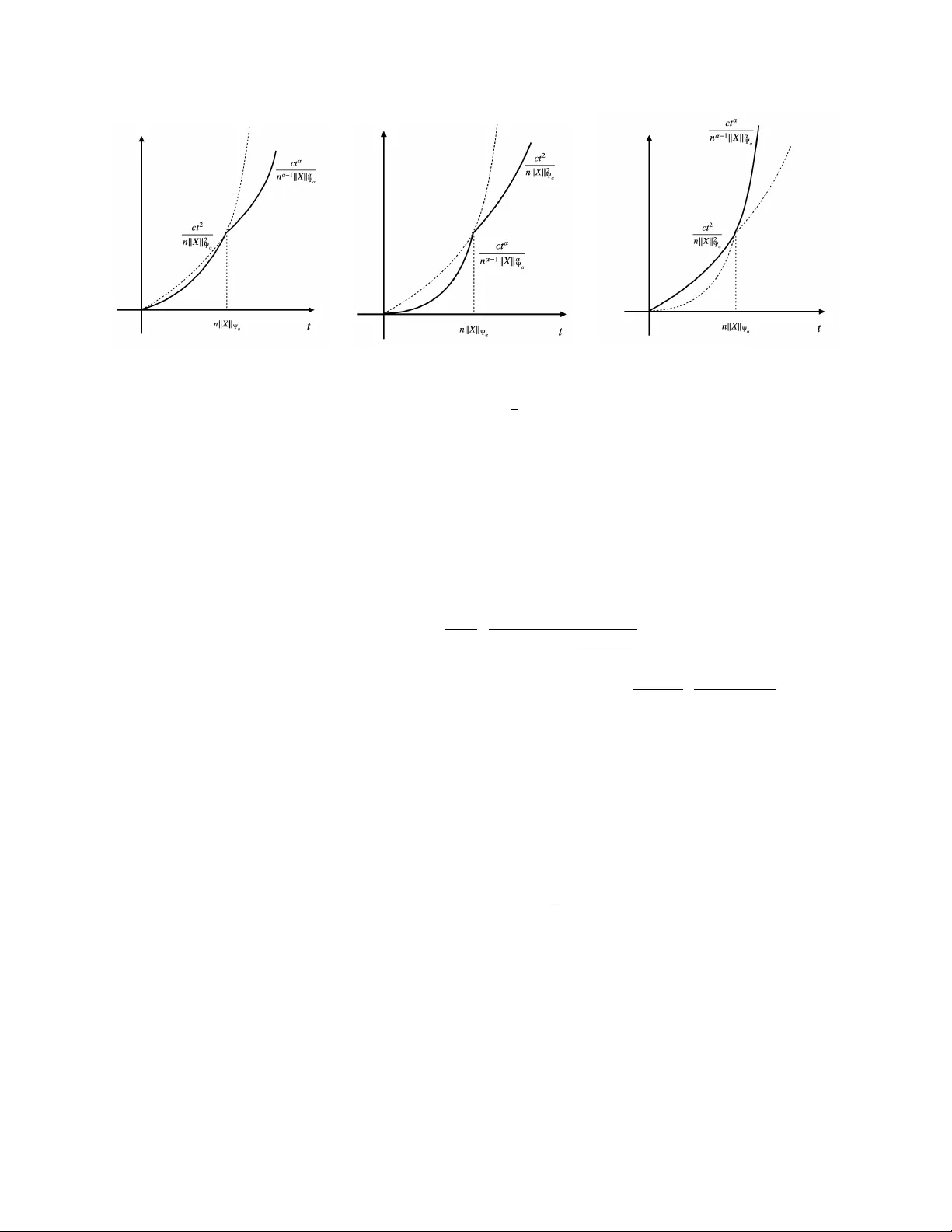
Sharp Concen tration Inequalities: Phase T ransition and Mixing of Orlicz T ails with V ariance ∗ Yinan Shen and Jinc hi Lv Univ ersity of Southern California Marc h 30, 2026 Abstract In this w ork, we in vestigate how to develop sharp concen tration inequalities for sub-W eibull random v ariables, including sub-Gaussian and sub-exp onen tial distributions. Although the ran- dom v ariables may not b e sub-Guassian, the tail probability around the origin behav es as if they were sub-Gaussian, and the tail probability deca ys align with the Orlicz Ψ α -tail else- where. Sp ecifically , for indep endent and identically distributed (i.i.d.) { X i } n i =1 with finite Orlicz norm ∥ X ∥ Ψ α , our theory unv eils that there is an interesting phase transition at α = 2 in that P ( | P n i =1 X i | ≥ t ) with t > 0 is upp er b ounded b y 2 exp  − C max n t 2 n ∥ X ∥ 2 Ψ α , t α n α − 1 ∥ X ∥ α Ψ α o for α ≥ 2, and by 2 exp  − C min n t 2 n ∥ X ∥ 2 Ψ α , t α n α − 1 ∥ X ∥ α Ψ α o for 1 ≤ α ≤ 2 with some positive constan t C . In many scenarios, it is often necessary to distinguish the standard deviation from the Orlicz norm when the latter can exceed the former greatly . T o accommo date this, we build a new theoretical analysis framework, and our sharp, flexible concentration inequalities inv olve the v ariance and a mixing of Orlicz Ψ α -tails through the min and max functions. Our theory yields new, impro ved concentration inequalities ev en for the cases of sub-Gaussian and sub- exp onen tial distributions with α = 2 and 1, resp ectiv ely . W e further demonstrate our theory on martingales, random vectors, random matrices, and cov ariance matrix estimation. These sharp concen tration inequalities can emp o wer more precise non-asymptotic analyses across different statistical and machine learning applications. Keywor d: sharp concentration inequalities, sub-W eilbull distributions, sub-Gaussian and sub- exp onen tial distributions, Orlicz tails, V ariance and moments, Martingales and random matrices, Co v ariance matrix estimation ∗ Yinan Shen is Assistan t Professor, R TPC (in fact postdo c) in Departmen t of Mathematics, Universit y of Southern California, Los Angeles, CA 90089 (E-mail: yinanshe@usc.e du ; ORCID: 0000-0001-9146-9549). Jinchi Lv is Kenneth King Stonier Chair in Business Administration and Professor, Data Sciences and Op erations Department, Marshall Sc ho ol of Business, Universit y of Southern California, Los Angeles, CA 90089 (E-mail: jinchilv@marshal l.usc.e du ; OR CID: 0000-0002-5881-9591). 1 1 In tro duction Concen tration inequalities are cen tral to mo dern statistics and mac hine learning, esp ecially in problems where tail probabilities determine finite-sample p erformance, suc h as matrix analysis ( Minsk er , 2017 ; Koltc hinskii and Xia , 2016 ; Adamczak et al. , 2011 ), decision-making and inference ( Hao et al. , 2019 ; Khamaru et al. , 2025 ; Lin et al. , 2025 ), and robust statistics ( Minsker , 2018 ; Dep ersin and Lecu´ e , 2022 ; Ma et al. , 2024 ). The goal of this pap er is to study concentration inequalities for real-v alued sub-W eibull random v ariables, i.e., random v ariables X whose tails deca y at an exp onential–W eibull rate P ( | X | ≥ t ) ≤ 2 exp  − t α K  , where K , α > 0 are constan ts, and t > 0. The case of α = 2 corresponds to sub-Gaussian distributions, while the case of α = 1 corresp onds to sub-exp onen tial distributions. Throughout the pap er, we work with random v ariables ha ving finite Orlicz Ψ α -norm, defined as follows. Definition 1 (Orlicz ∥ · ∥ Ψ α -norm) . F or a given r andom variable X and α ≥ 1 , we define the Orlicz ∥ · ∥ Ψ α -norm as ∥ X ∥ Ψ α := inf u> 0 { E { exp( | X | /u ) α } ≤ 2 } . A large literature has con tributed to dev eloping concentration theory for sub-W eibull random v ariables; see, e.g., Bennett ( 1962 ), T alagrand ( 1989 ), T alagrand ( 1994 ), Latala ( 1997 ), Boucheron et al. ( 2003 ), Koltc hinskii ( 2011 ), Adamczak et al. ( 2011 ), v an de Geer and Lederer ( 2013 ), Ledoux and T alagrand ( 2013 ), Rio ( 2013 ), Minsker ( 2017 ), V ershynin ( 2018 ), Hao et al. ( 2019 ), Zhang and W ei ( 2022 ), Kuchibhotla and Chakrab ortty ( 2022 ), Jeong et al. ( 2022 ), and references therein. Y et for the fundamen tal tail probabilit y P      n X i =1 X i      ≥ t ! for random v ariables X i ’s and t > 0, the existing results in the literature still leav e an imp ortan t gap. On the one hand, for α > 2, existing concen tration inequalities either require information str onger than ∥ X ∥ Ψ α < ∞ or fail to deliver a sharp Ψ α large-deviation tail. On the other hand, when the Orlicz norm ∥ X ∥ Ψ α and the standard deviation σ X are not of the same order, the literature does not simultaneously capture the v ariance-dominated small-deviation regime and the correct Ψ α -tail for large deviations. Sp ecifically , for α > 2, Ledoux and T alagrand ( 2013 ) and T alagrand ( 1989 ) pro ved the elegan t inequalit y      n X i =1 X i      Ψ α ≤ K α      n X i =1 X i      1 +    ∥ X i ∥ Ψ s    β , ∞ ! , (1) 2 where α < s < ∞ . How ev er, ∥ X i ∥ Ψ s do es not need to b e finite: it is p ossible to ha v e ∥ X i ∥ Ψ s = ∞ while still ha ving ∥ X ∥ Ψ α < ∞ . In that case, ( 1 ) b ecomes trivial for b ounding the Ψ α -norm of P n i =1 X i . F or α ∈ [1 , 2], the same line of w ork established that      n X i =1 X i      Ψ α ≤ K α        n X i =1 X i      1 + n X i =1 ∥ X i ∥ β Ψ α ! 1 β   , (2) whic h has a particularly clean form, but still do es not separate the role of v ariance from that of the Orlicz norm and as we will demonstrate later, Orlicz norm is not alwa ys a sharp characterization of tail probability . F rom a differen t persp ectiv e, the foundational w ork of Koltchinskii ( 2011 ) sho wed that for α ≥ 1, P      n X i =1 X i      ≥ t ! ≤ 2 exp   − C min    t 2 nσ 2 X , t ∥ X ∥ Ψ α log 1 α  2 ∥ X ∥ Ψ α σ X       , (3) whic h is sharp for sufficien tly small deviations since it preserves the v ariance term. Ho wev er, it yields only a sub-exp onen tial tail for P n i =1 X i regardless of α ≥ 1. A t the same time, the crude triangle inequalit y      n X i =1 X i      Ψ α ≤ n ∥ X ∥ Ψ α < ∞ sho ws that P n i =1 X i still has finite Ψ α -norm under the assumption of ∥ X ∥ Ψ α < ∞ . Although this b ound is far from sharp, it strongly suggests that a sharp er concentration theory should exist. This motiv ates the follo wing questions: F or the tail pr ob ability P ( | P n i =1 X i | ≥ t ) , c an one obtain a sharp Ψ α -tail under only ∥ X i ∥ Ψ α < ∞ while simultane ously r etaining varianc e-c ontr ol le d c onc entr ation for sufficiently smal l t ? Mor e br o ad ly, what is the c orr esp onding c onc entr ation the ory when X 1 , · · · , X n ar e dep endent? In this paper, w e aim to answer these questions and iden tify a sharp phase transition at α = 2 in univ ariate sub-W eibull concentration. The central no velt y of our work is that sums of Ψ α random v ariables displa y lo cal sub-Gaussian b eha vior around the origin even when the summands themselv es are not sub-Gaussian, while their large-deviation b eha vior retains the correct Ψ α -tail. This yields a sharp, density-free concen tration theory in the regime of α ≥ 2, and Section 3 further dev elops a v ariance-sensitive theory that remains statistically optimal when ∥ X ∥ Ψ α and σ X are not comparable. The corollary b elow illustrates the main phenomenon in the indep enden t and iden tically distributed (i.i.d.) setting. 3 Corollary 1 (Concentration for i.i.d. univ ariate) . Assume that X 1 , · · · , X n ar e i.i.d. me an-zer o r e al-value d r andom variables, and satisfy ∥ X ∥ Ψ α < ∞ for some α ≥ 1 . Then we have that P      n X i =1 X i      ≥ t ! ≤ 2 exp − C max ( t 2 n ∥ X ∥ 2 Ψ α , t α n α − 1 ∥ X ∥ α Ψ α )! for α ≥ 2 , P      n X i =1 X i      ≥ t ! ≤ 2 exp − C min ( t 2 n ∥ X ∥ 2 Ψ α , t α n α − 1 ∥ X ∥ α Ψ α )! for 1 ≤ α ≤ 2 , (4) wher e C > 0 is some c onstant that do es not dep end on α , t, n, X . Corollary 1 ab o ve is a direct consequence of Theorem 1 (see Section 2 ) and already shows wh y the new theory differs qualitativ ely from the existing literature. When α ≥ 2, the decisiv e feature of ( 4 ) is the appearance of max , rather than the familiar min in Boucheron et al. ( 2003 ); Kuchibhotla and Chakrab ortt y ( 2022 ); Zhang and W ei ( 2022 ); this is precisely the phase transition at α = 2 and it yields a strictly sharp er tail in the large-deviation regime. When 1 ≤ α ≤ 2, the b ound reco vers the correct order when ∥ X ∥ Ψ α ≍ σ X . In b oth regimes, the sum is lo cally sub-Gaussian: for all α ≥ 1 and t ≤ n ∥ X ∥ Ψ α , P      n X i =1 X i      ≥ t ! ≤ 2 exp − C t 2 n ∥ X ∥ 2 Ψ α ! , while for t ≥ n ∥ X ∥ Ψ α , P      n X i =1 X i      ≥ t ! ≤ 2 exp − C t α n α − 1 ∥ X ∥ α Ψ α ! , whic h is consisten t with the fact that P n i =1 X i has finite Ψ α -norm and sharpens substantially the crude triangle inequalit y . A t the moment lev el, w e prov e that E (      1 √ n n X i =1 X i      p ) ≤ C p 1 p p 2 ∥ X ∥ p Ψ α + C p α 1 p p α n p 2 − p α ∥ X ∥ p Ψ α · exp( − cn ) when α ≥ 1 , E (      1 √ n n X i =1 X i      p ) ≤ C p min n p p 2 , p p α n p 2 − p α o · ∥ X ∥ p Ψ α when α ≥ 2 , whic h is unimprov able up to universal constan ts. These moment b ounds impro ve the results in Kuc hibhotla and Chakrab ortt y ( 2022 ); Latala ( 1997 ) in tw o distinct regimes: 1) when α > 2 and 2) when α ∈ [1 , 2] with 1 ≪ n ≲ p . W e defer the detailed discussion of concentration, moments, and Ψ α -norms for heterogeneous univ ariate summands to Section 2 . Man y imp ortan t distributions satisfy that σ X ≪ ∥ X ∥ Ψ α , so separating the v ariance from the Orlicz norm is essential rather than superficial. A basic example is the Bernoulli random v ariable with success probability close to zero. T o handle this regime, we in tro duce Definition 2 (see Section 4 3 ), a general moment framew ork that extends the sub-Gaussian characterizations in v an de Geer and Lederer ( 2013 ) and Alquier and Biau ( 2013 ). This framework in teracts naturally with the class of random v ariables ha ving finite Ψ α -norm. In particular, giv en i.i.d. X 1 , · · · , X n with ∥ X ∥ Ψ α < ∞ , w e sho w that there are infinitely many choices of ( σ, L ) satisfying Definition 2 ; for suitable choices, w e can obtain that for all α ≥ 1, P      n X i =1 X i      ≥ t ! ≤ 2 exp  − C 1 t 2 nσ 2 X  for t ≤ cn σ 2 X ∥ X ∥ Ψ α  log  2 ∥ X ∥ Ψ α σ X  − 1 α , P      n X i =1 X i      ≥ t ! ≤ 2 exp − C 1 t α n α − 1 ∥ X ∥ α Ψ α ! for t ≥ n ∥ X ∥ Ψ α , and for t b et ween these tw o scales, the tail b ecomes an in terp olation of Ψ 1 - and Ψ 2 -tails that connects the t wo endp oin ts. In particular, when α = 1, the second endp oin t b ecomes t ≥ nσ X . W e defer the details to Theorem 3 and C orollary 4 (see Section 3 ). These results preserv e the sharp v ariance scaling of Koltc hinskii ( 2011 ) for small deviations while reco vering the missing sharp Ψ α - tail for large deviations. In this sense, our results sharp en the w orks of T alagrand ( 1994 ), Ledoux and T alagrand ( 2013 ), Kuchibhotla and Chakrab ortt y ( 2022 ), and complete the picture initiated b y Koltc hinskii ( 2011 ). Our framew ork also extends b eyond indep enden t scalar sums. F or martingales, we study the distribution of the limit lim n →∞ P n k =1 a k X k , where { X k } is a martingale. Our goal is differen t from that of Rio ( 2013 ), which con trolled the limiting distribution under an assumed moment generating function b ound. In con trast, w e derive the relev ant moment generating function b eha vior and con vergence from moment conditions or from a finite conditional Ψ α -norm. F or random v ectors, w e iden tify a differen t t wo-phase transition, now at α = 4, separating the regimes of 2 ≤ α ≤ 4 and α ≥ 4. The resulting concen tration b eha vior exhibits a non trivial in terplay among the deca ying Ψ 2 - , Ψ 4 -, Ψ α 2 -, and Ψ α -tails, together with a delicate in teraction b et ween the v ariance and Ψ α -norm. These results sharp en and extend Theorem 3.1.1 in the classical work of V ershynin ( 2018 ) and the recen t w ork of Jeong et al. ( 2022 ). The state-of-the-art Jeong et al. ( 2022 ) pro ved a sharp bound for X ∈ R d with i.i.d. comp onen ts and v ar( X i ) = 1, K := ∥ X i ∥ Ψ 2 ≥ 1,    ∥ X ∥ − √ d    Ψ 2 ≤ C K √ log K , whic h implies that P     ∥ X ∥ − √ d    ≥ t  ≤ 2 exp  − C t 2 K 2 log K  . 5 W e pro ve the sharp er tail probabilit y P     ∥ X ∥ − √ dσ X    ≥ s  ≤                    2 exp   − cs 2 ∥ X ∥ 2 Ψ 2 log  2 ∥ X ∥ Ψ 2 σ X    for 0 < s ≤ τ 1 , 2 exp  − cs 4 dσ X ∥ X ∥ 3 Ψ α  for τ 1 ≤ s ≤ τ 2 , 2 exp  − cs 2 ∥ X ∥ 2 Ψ 2  for s ≥ τ 2 , where τ 1 := √ d s σ X ∥ X ∥ Ψ 2 log  2 ∥ X ∥ Ψ 2 σ X  and τ 2 := √ d p σ X ∥ X ∥ Ψ 2 . The same framew ork also applies to eigen v alue analysis for random matrices and cov ariance matrix estimation; see Section 4 . 1.1 Related w orks The discussion ab o v e already identifies the ma jor gap in the literature. W e now p osition our results more systematically relative to the existing works. An early foundational w ork is T alagrand ( 1994 ), which studied concentrations of symmetric random v ariables with densit y c α exp( −| x | α ) and obtained the moment generating function bound E exp( λX ) ≤ exp( C α λ 2 E exp( | X | /C )) for all λ ≤ 1 , E exp( λX ) ≤ exp( λ β /β + log ( E exp( | X | α /C α ))) for all λ > 0 . (5) Here, β is the conjugate of α , i.e., 1 α + 1 β = 1. F or the symmetric density mo del considered in T alagrand ( 1994 ), the b ound is sharp, but for general random v ariables—esp ecially asymmetric ones and for sufficien tly small λ —( 5 ) is not sharp or sufficien t. The generalizations of Ledoux and T alagrand ( 2013 ) and T alagrand ( 1989 ) led to ( 1 ) and ( 2 ). As discussed ab o v e, how ev er, ( 1 ) may b e v acuous when α > 2, while ( 2 ) does not separate the v ariance from the Orlicz norm. A second line of work includes Bouc heron et al. ( 2003 ), Adamczak et al. ( 2011 ), Kuchibhotla and Chakrab ortty ( 2022 ), and Zhang and W ei ( 2022 ). These pap ers pro ved that for all α ∈ [1 , ∞ ), P      n X i =1 X i      ≥ C √ n ∥ X ∥ Ψ α √ t + C n 1 β ∥ X ∥ Ψ α t 1 α ! ≤ 2 exp ( − t ) , (6) whic h yields a sub-Gaussian comp onen t along with a Ψ α comp onen t. How ever, for α ≥ 2 this is still a standard min-type b ound and therefore, misses the sharp er max-t yp e b eha vior established in Theorem 1 . Moreo ver, Latala ( 1997 ), Kuc hibhotla and Chakrab ortt y ( 2022 ), and Zhang and W ei ( 2022 ) established or employ ed the moment inequalit y E (      1 √ n n X i =1 X i      p ) ≤ C p 2 1 p p 2 ∥ X ∥ p Ψ α + C p α 1 p p α n p β − p α ∥ X ∥ p Ψ α for α ≥ 1 , 6 log( 1 2 P ( | P n k =1 X k | ≥ t )) α ≥ 2 Ledoux and T alagrand ( 2013 ) −  t K α ∥ P k X i ∥ 1 + ∥ ( ∥ X k ∥ Ψ s ) ∥ β , ∞  α Bouc heron et al. ( 2003 ) − C α min  t 2 n ∥ X ∥ 2 Ψ α , t α n α − 1 ∥ X ∥ α Ψ α  + C ′ α Koltc hinskii ( 2011 ) − C min    t 2 nσ 2 X , t ∥ X ∥ Ψ α log  2 ∥ X ∥ Ψ α σ X     Kuc hibhotla and Chakrab ortt y ( 2022 ) − C min  t 2 n ∥ X ∥ 2 Ψ α , t α n α − 1 ∥ X ∥ α Ψ α  This work (Theorem 1 ) − C max  t 2 n ∥ X ∥ 2 Ψ α , t α n α − 1 ∥ X ∥ α Ψ α  This work (distinguishing ∥ X ∥ Ψ α and σ X ) Section 3 T able 1: Concen tration inequalities when α ≥ 2. Here, K α , C α , C ′ α represen t p ositiv e constants that may dep end on α , follo wing the notation in the original works, while p ositiv e constant C do es not dep end on α, X , n . whic h is gov erned by the maxim um of C p 2 1 p p 2 ∥ X ∥ Ψ α and C p α 1 p p α n p β − p α ∥ X ∥ Ψ α . This line of w ork do es not distinguish σ X from ∥ X ∥ Ψ α . Consequently , ( 6 ) is sharp for α ∈ [1 , 2] when σ X ≍ ∥ X ∥ Ψ α , but is not sharp for α > 2 and is not v ariance-sensitiv e when σ X ≪ ∥ X ∥ Ψ α . A third line of work, represented b y Koltchinskii ( 2011 ) and Adamczak ( 2008 ), emphasizes the v ariance-controlled concentration around the origin. In addition to Koltchinskii ( 2011 ), Adamczak ( 2008 ) dev elop ed a related concen tration inequality at α = 1 that is also adaptive to v ariance near the origin, but incurs an additional log( n ) factor for sufficien tly large deviations. The approaches in Koltc hinskii ( 2011 ) and Adamczak ( 2008 ) are complementary , and either can b e sharp er dep ending on the specific regime. Our contribution is to unify sharp local v ariance b eha vior with the correct global Ψ α -tail in a single framework. T o appreciate these sharp er b ounds, T ables 1 and 2 summarize representativ e concentration inequalities for univ ariate random v ariables. The comparison mak es the contribution of this pap er transparen t. When α > 2, the a v ailable b ounds are either p oten tially v acuous or retain a min-t yp e tail; in contrast, Theorem 1 yields the sharp max-type b eha vior in T able 1 . When α ∈ [1 , 2], Theorem 1 matc hes the b est known order when σ X ≍ ∥ X ∥ Ψ α , while the inequalities in Section 3 sharp en the literature whenever σ X needs to b e separated from ∥ X ∥ Ψ α . Although our technical argumen ts are self-contained and do not rely directly on existing results, the cited w orks provide a ric h source of elegant ideas that motiv ate our analysis. F or concentration inequalities of b ounded random v ariables, w e refer in terested readers to Ahlswede and Winter ( 2002 ), Rech t ( 2011 ), Gross et al. ( 2010 ), and Gross ( 2011 ). 7 log( 1 2 P ( | P n k =1 X k | ≥ t )) 1 ≤ α ≤ 2 Ledoux and T alagrand ( 2013 ) −  t K α ∥ P k X i ∥ 1 + n 1 − 1 α ∥ X ∥ Ψ α  α Bouc heron et al. ( 2003 ) − C α min  t 2 n ∥ X ∥ 2 Ψ α , t α n α − 1 ∥ X ∥ α Ψ α  + C ′ α Koltc hinskii ( 2011 ) − C min    t 2 nσ 2 X , t ∥ X ∥ Ψ α log  2 ∥ X ∥ Ψ α σ X     Kuc hibhotla and Chakrab ortt y ( 2022 ) − C min  t 2 n ∥ X ∥ 2 Ψ α , t α n α − 1 ∥ X ∥ α Ψ α  This work (Theorem 1 ) − C min  t 2 n ∥ X ∥ 2 Ψ α , t α n α − 1 ∥ X ∥ α Ψ α  This work (distinguishing ∥ X ∥ Ψ α and σ X ) Section 3 T able 2: Concentration inequalities when 1 ≤ α ≤ 2. Here, K α , C α , C ′ α represen t p ositiv e constants that may dep end on α , follo wing the notation in the original works, while p ositiv e constant C do es not dep end on α, X , n . When σ X ≍ ∥ X ∥ Ψ α , our result aligns with Kuchibhotla and Chakrabortty ( 2022 ); when σ X ≪ ∥ X ∥ Ψ α , Section 3 is sharp er than the existing literature. 1.2 Our con tributions W e summarize the ma jor contributions in the same order as the pap er. First, Lemmas 1 and 3 establish new momen t generating function b ounds that improv e and generalize T alagrand ( 1994 ). These lemmas are the analytical core of the pap er and explain the phase transition at α = 2 through the regularity of the moment generating function. Building on them, Section 2 prov es refined concentration, moment, and Orlicz norm b ounds for sums of indep enden t random v ariables with ∥ X ∥ Ψ α < ∞ . F or sufficiently small deviation t , the tail probability P ( | P X i | ≥ t ) is sub- Gaussian, whereas for large enough t , it has the correct Ψ α -tail. In the regime of ∥ X ∥ Ψ α ≍ σ X , these b ounds are optimal. T o the b est of our kno wledge, this is the first work to prov e a sharp, densit y-free concentration inequalit y with a genuine Ψ α -tail for α ≥ 2 under the only assumption of ∥ X ∥ Ψ α < ∞ , thereby impro ving the state of the art in Kuc hibhotla and Chakrab ortty ( 2022 ). Figure 1 visualizes such impro vemen t. Second, Section 3 dev elops the v ariance-sensitive framework based on Definition 2 . When α = 2, suc h framework reduces to conditions considered previously in v an de Geer and Lederer ( 2013 ) and Alquier and Biau ( 2013 ); for general α , it yields a new interpolation b et ween the v ariance and Ψ α -tails. Our main results, Theorem 3 and Corollary 4 , sim ultaneously pro duce sub-Gaussian tails dep ending only on v ariance for sufficien tly small t , and rate-optimal Ψ α -tails for large t , ev en though the random v ariables themselves may not b e sub-Gaussian. This com bination c annot be 8 (a) α ∈ [1 , 2] (b) α ≥ 2 (c) α ≥ 2 Figure 1: The y -axis represen ts the b ound on − log ( 1 2 P ( | P n i =1 X i | ≥ t )). Figures 1a and 1b are from Kuchibhotla and Chakrab ortt y ( 2022 ). Figure 1c corresp onds to Theorem 1 or Theorem 3 when σ X do es not need to b e distinguished from ∥ X ∥ Ψ α . The b ound in Figure 1c impr oves that in Figure 1b . reco vered by simply combining previous inequalities. In particular, for sub-exp onen tial random v ariables, w e prov e that P      n X i =1 X i      ≥ t ! ≤ 2 exp   − max    min    t 2 nσ 2 X , t ∥ X ∥ Ψ 1 log  2 ∥ X ∥ Ψ 2 σ X     , min  t ∥ X ∥ Ψ 1 , t 2 nσ X ∥ X ∥ Ψ 1  , whic h c annot be obtained from the existing literature and impro ves, e.g., the Bernstein-type bounds suc h as those discussed in V ershynin ( 2018 ). More generally , for all α ≥ 1, Corollary 4 yields sub- Gaussian tails of form exp − ct 2 / n X i =1 v ar( X i ) ! for sufficiently small t , while for large t , the tail probability b ecomes exp − ct α / ( n X i =1 ∥ X i ∥ β Ψ α ) α β ! , whic h is rate-optimal. These results sharp en T alagrand ( 1989 , 1994 ); Ledoux and T alagrand ( 2013 ); Bouc heron et al. ( 2003 ); Kuchibhotla and Chakrab ortt y ( 2022 ) and complete Koltc hinskii ( 2011 ). Figure 2 compares the corresp onding tails. Third, Section 4 extends the framework to martingales for dep endent data, random vectors, random matrices, and co v ariance matrix estimation. These extensions sho w that our new theoretical 9 (a) α ≥ 1 (b) α ∈ [1 , 2] (c) α ≥ 2 Figure 2: The y -axis represen ts the b ound on − log ( 1 2 P ( | P n i =1 X i | ≥ t )). Figure 2a plots the b ound giv en by Koltc hinskii ( 2011 ), whose tail probability is sharp when t ≤ nσ 2 X ∥ X ∥ Ψ α log 1 α  ∥ X ∥ Ψ α σ X  . Figures 2b and 2c corresp ond to Theorem 3 and Corollary 3 . The b ounds in Figures 2b and 2c impr ove those in Figures 1a , 1b , and 2a . framew ork is not limited to an isolated scalar setting: it is flexible enough to impro ve existing v ector and matrix norm b ounds, including those of V ershynin ( 2018 ) and Jeong et al. ( 2022 ), even in some i.i.d. sub-Gaussian settings when σ X ≪ ∥ X ∥ Ψ α . The resulting sharp er tails are relev an t to statistical and mac hine learning applications such as low-rank matrix recov ery ( Koltchinskii , 2011 ), adaptiv ely collected data ( Lin et al. , 2025 ; Khamaru et al. , 2025 ), and tensor learning ( Zhang and Xia , 2018 ; Zhou and Chen , 2025 ; Ab dalla and V ershynin , 2026 ). Section 5 discusses further implications and p ossible extensions of the theory . All pro ofs of the main results and additional tec hnical details are included in the Supplemen tary Material. Notation . Throughout the pap er, for any random v ariable X and num b er k ≥ 0, we define ∥ X ∥ k :=  E | X | k  1 k , and v ar( X ) denotes the v ariance of X . F or a v ector X ∈ R d , denote b y ∥ X ∥ its Euclidean norm, and for a matrix X , denote by ∥ X ∥ its ope rator norm. Univ ersal constan ts are written as C , C 1 , C 2 , c, c 1 , · · · . In addition, [ a ] denotes the largest integer not exceeding a , and for a nonnegative in teger k , w e define 0! = 1 and k ! = k × ( k − 1) × · · · × 1. 2 Concen tration inequalities when Orlicz norm is prop ortional to standard deviation T o illustrate our main ideas, we start with concentration inequalities for indep enden t univ ariate sub-W eibull random v ariables, when it is not ne c essary to emphasize the difference b et ween the 10 Orlicz norm ∥ X ∥ Ψ α and the standard deviation σ X := p v ar( X ). The lemma b elow upp er b ounds the moment generating function for general sub-W eibull random v ariables with α > 1. Lemma 1 (Momen t generating function) . L et X b e a me an-zer o r andom variable with ∥ X ∥ Ψ α < ∞ for some α > 1 , and β the c onjugate of α with 1 α + 1 β = 1 . Then ther e exist some p ositive c onstants C, C 1 , C 2 , C 3 , C 4 , C 5 that do not dep end on α , λ , and X such that for any λ ≥ 0 , (1) for α ≥ 2 , it holds that E { exp( λX ) } ≤ exp  C 1 min n λ 2 ∥ X ∥ 2 Ψ α , λ β ∥ X ∥ β Ψ α o ; (2) for α ∈ (1 , 2] , it holds that E { exp( λX ) } ≤ exp( C 2 β λ 2 ∥ X ∥ 2 Ψ α ) when λ ≤ 1 / ( C ∥ X ∥ Ψ α ) , E { exp( λX ) } ≤ exp( C β 3 β λ β ∥ X ∥ β Ψ α ) when λ ≥ 1 / ( C ∥ X ∥ Ψ α ); and further it holds for any τ ∈ (0 , 1) that E { exp( λX ) } ≤ exp  C 4 1 1 − τ λ 2 ∥ X ∥ 2 Ψ α  when λ ≤ τ / ( C ∥ X ∥ Ψ α ) , E { exp( λX ) } ≤ exp C β 5 τ − [ β ] − 1 1 − τ λ β ∥ X ∥ β Ψ α ! when λ ≥ τ / ( C ∥ X ∥ Ψ α ) . Lemma 1 ab ov e sho ws that for α > 1, regardless of α ≥ 2 or α ∈ (1 , 2], when λ is sufficiently small, the moment generating function can b e upp er b ounded with exp( O ( λ 2 ∥ X ∥ 2 Ψ α )); when λ is sufficiently large, the b ound for the moment generating function b ecomes exp( O ( λ β ∥ X ∥ β Ψ α )). Lemma 1 impr oves and c ompletes the moment generating function b ound in T alagrand ( 1994 ) or ( 5 ). The following lemma pro vides the lo wer b ound on the momen t generating function for λ with sufficien tly small v alues. Lemma 2 (Low er b ound on momen t generating function) . L et X b e a me an-zer o r andom vari- able with ∥ X ∥ Ψ α < ∞ for some α ≥ 1 , and σ 2 X := v ar( X ) . Then we have that for al l λ ≤ 1 ∥ X ∥ Ψ α  log  2 ∥ X ∥ Ψ α σ X  − 1 α , E { exp( λX ) } ≥ exp  λ 2 σ 2 X / 8  . Consequen tly , combining Lemma 1 and Lemma 2 v erifies that for sufficien tly small λ , it holds that log( E ( λX )) ≍ λ 2 , 11 whic h is quadratic in λ . In fact, w e will demonstrate in Example 1 and Theorem 3 in Section 3 later that log( E ( λX )) ≍ λ 2 σ 2 X holds in this range. It implies that regardless of v alues of α , for small enough λ , the m omen t generating function of X b eha ves as if the random v ariable were sub- Gaussian with the Orlicz norm prop ortional to the standard deviation. An application of Lemma 1 yields the follo wing concentration inequalities. Theorem 1 (Concen tration inequalities) . L et X 1 , · · · , X n b e indep endent me an-zer o r andom vari- ables with ∥ X i ∥ Ψ α < ∞ , a 1 , · · · , a n any n sc alars, and β satisfy 1 α + 1 β = 1 . Then ther e exist some c onstants C 1 , C 2 > 0 that do not dep end on α , t , and X such that for α ≥ 2 , P      n X i =1 a i X i      ≥ t ! ≤ 2 exp − C 1 max ( t 2 P n i =1 a 2 i ∥ X i ∥ 2 Ψ α , t α ( P n i =1 | a i | β ∥ X i ∥ β Ψ α ) α β )! , and for 1 ≤ α ≤ 2 , P      n X i =1 a i X i      ≥ t ! ≤ 2 exp − C 2 min ( t 2 P n i =1 a 2 i ∥ X i ∥ 2 Ψ α , t α ( P n i =1 | a i | β ∥ X i ∥ β Ψ α ) α β )! , for al l t ≥ 0 . Theorem 1 ab ov e establishes the concen tration inequalities for sub-W eibull random v ariables. It unv eils an interesting phase transition at α = 2. Regardless of α ∈ [2 , ∞ ) or α ∈ [1 , 2], for sufficien tly small t , the tail probability of P n i =1 a i X i b eha v es as if { X i } n i =1 w ere sub-Gaussian. When t is large enough, the tail probability presented in Theorem 1 enjo ys a Ψ α deca ying tail. Indeed, the triangle inequality with resp ect to the Ψ α -norm leads to      n X i =1 a i X i      Ψ α ≤ n X i =1 | a i | ∥ X i ∥ Ψ α , whic h entails that P n i =1 a i X i has a finite Ψ α -norm. This is consistent with Theorem 1 , while Theorem 1 sharp ens the triangle inequality . In addition, when α = 1, we hav e β = ∞ and ( P n i =1 | a i | β ∥ X i ∥ β Ψ 1 ) 1 β = max i =1 , ··· ,n | a i |∥ X i ∥ Ψ 1 . The following theorem provides the moment inequalities for P n i =1 a i X i . Theorem 2 (Momen t inequalities) . L et X 1 , · · · , X n b e indep endent me an-zer o r andom variables with ∥ X i ∥ Ψ α < ∞ for some α ≥ 1 , a 1 , · · · , a n any n sc alars, and p ≥ 1 . Then we have that for al l α ≥ 1 , E (      n X i =1 a i X i      p ) ≤ C p 1 p p 2 n X i =1 a 2 i ∥ X i ∥ 2 Ψ α ! p 2 + C p 1 p p α n X i =1 a β i ∥ X i ∥ β Ψ α ! p β exp    − C   ( P n i =1 | a i | β ∥ X ∥ β Ψ α ) 1 β ( P n i =1 a 2 i ∥ X i ∥ 2 Ψ α ) 1 2   2 α α − 2    , 12 and additional ly for al l α ≥ 2 , E (      n X i =1 a i X i      p ) ≤ C p 2 min    p p 2 n X i =1 a 2 i ∥ X i ∥ 2 Ψ α ! p 2 , p p α n X i =1 | a i | β ∥ X i ∥ β Ψ α ! p β    , wher e c onstants C, C 1 , C 2 > 0 do not dep end on α , p , and { X i } n i =1 . Theorem 2 ab ov e pro vides upp er b ounds for the p th momen t of P n i =1 a i X i . Sp ecifically , in the con text of i.i.d. X i ’s with equal weigh ts, Theorem 2 implies that for all α ≥ 1 and all p ≥ 1, E (      1 √ n n X i =1 X i      p ) ≤ C p 1 p p 2 ∥ X ∥ p Ψ α + C p 1 p p α n p 2 − p α ∥ X ∥ p Ψ α · exp( − cn ) . Hence, for each fixed p , when σ X ≍ ∥ X ∥ Ψ α , the right-hand side of the expression ab o ve is domi- nated b y C p 1 p p 2 ∥ X ∥ p Ψ α ≍ C p 1 p p 2 σ p X as n → ∞ , which is consistent with the central limit theorem. Mean while, for p v arying with n and the scenario of α ≤ 2, when p ≤ n the upp er bound is domi- nated by p p 2 , whereas when p ≥ n the upp er b ound is dominated by p p α . Moreo ver, for the scenario of α ≥ 2, Theorem 2 entails the following upp er b ound E (      1 √ n n X i =1 X i      p ) ≤ C p min n p p 2 , p p α n p 2 − p α o · ∥ X ∥ p Ψ α , where X i ’s are i.i.d. The ab o ve inequality shows that for α ≥ 2, when p ≤ n it is b ounded by C p 2 1 p p 2 , while when n ≤ p it is bounded b y C p α 1 p p α n p 2 − p α . A com bination of Theorem 1 and Theorem 2 further yields the following b ound for the Orlicz norm. Corollary 2 (Bound on Orlicz norm) . L et X 1 , · · · , X n b e indep endent me an-zer o r andom variables with ∥ X i ∥ Ψ α < ∞ , and a = ( a 1 , · · · , a n ) any n -dimensional ve ctor. Then we have that for α ≥ 2 ,      n X i =1 a i X i      Ψ α ≤ C 1 n X i =1 | a i | β ∥ X i ∥ β Ψ α ! 1 β ,      n X i =1 a i X i      Ψ 2 ≤ C 1 n X i =1 a 2 i ∥ X i ∥ 2 Ψ α ! 1 2 , and for α ∈ [1 , 2] ,      n X i =1 a i X i      Ψ α ≤ C 2 n X i =1 a 2 i ∥ X i ∥ 2 Ψ α ! 1 2 , wher e C 1 , C 2 > 0 ar e c onstants that do not dep end on α , a , and X . Corollary 2 ab o ve gives the upp er b ound for the Ψ α - and Ψ 2 -norms of P n i =1 a i X i , where the b ound is expressed explicitly b y coefficients a i and ∥ X i ∥ Ψ α . Similarly , a phase transition at α = 2 13 is observed. Generally , Corollary 2 is not impro v able, and when it is nece ssary to distinguish ∥ X ∥ Ψ α and σ X , a sharp er and mor e delic ate b ound is given in Corollary 3 in Section 3 later. T aken together, Theorem 1 , Theorem 2 , and Corollary 2 impr ove and c omplete the univ ariate concen tration inequalities in the w orks including Ledoux and T alagrand ( 2013 ), Boucheron et al. ( 2003 ), and Kuc hibhotla and Chakrab ortt y ( 2022 ), among others. Remark 1 (Characterization of concen tration) . A natur al question is what the appr opriate char- acterization of P n i =1 a i X i is. Inde e d, we pr ovide the tail pr ob ability in The or em 1 , the b ound of moments in The or em 2 , and its Ψ α -norm in Cor ol lary 2 . The tail pr ob ability in The or em 1 pr esents a delic ate interplay b etwe en Ψ 2 - and Ψ α -tails. We emphasize that it is not p ossible to obtain the delic ate tail pr ob ability in The or em 1 simply b ase d on the b ounds of the Ψ α -norm or moments. 3 Concen tration inequalities when Orlicz norm can exceed stan- dard deviation greatly In this section, we further inv estigate the concentration inequalities of sub-W eibull random v ari- ables when the Orlicz norm may not b e prop ortional to the standard deviation, in which the tail probabilit y b ounds established in Section 2 earlier may no longer be tight. Indeed, it holds that σ X := p v ar( X ) ≤ √ 2 ∥ X ∥ Ψ α for an y random v ariable X . Ho w ever, these t wo quan tities (i.e., the Orlicz norm and standard deviation) ma y not ha ve the same scale in general, e.g., for Bernoulli distributions; that is, the Orlicz norm can exceed the standard deviation greatly . This requires us to distinguish the standard deviation σ X from the Orlicz norm ∥ X ∥ Ψ α . Sp ecifically , w e now fo cus on random v ariables that are characterized b y moments, where the momen ts are determined join tly b y t w o positive quantities σ and L as sp ecified in the definition below. Definition 2. Ther e exist two p ositive c onstants σ and L such that for al l inte gers k ≥ 2 and some α ≥ 1 , it holds that E | X | k ≤ k k α σ 2 L k − 2 . Definition 2 ab o ve gives a delicate characterization of the distribution and has b een prev alent in the literature; see, e.g., v an de Geer and Lederer ( 2013 ) and Alquier and Biau ( 2013 ) for the condition under α = 2. Indeed, Definition 2 is related to the Orlicz Ψ α -norm; see the remark below. Remark 2. If a r andom variable X satisfies Definition 2 with some ( σ, L ) , its Orlicz Ψ α -norm c an b e b ounde d as ∥ X ∥ Ψ α ≤ C max { σ , L } . On the other hand, if a r andom variable X admits ∥ X ∥ Ψ α < ∞ , it satisfies Definition 2 with the choic e of ( σ, L ) = ( ∥ X ∥ Ψ α , C ∥ X ∥ Ψ α ) . 14 W e emphasize that σ ≪ L can indeed o ccur in man y scenarios. As a concrete example, consider a Bernoulli random v ariable X ∼ Ber( p ). Its cen tered momen ts scale with its v ariance, although its Orlicz norm remains b ounded b y an absolute constan t, i.e., E | X − E X | k = p (1 − p ) n p k − 1 + (1 − p ) k − 1 o . It shows that Ber( p ) satisfies Definition 2 with σ = p p (1 − p ) and L = 1. More generally , for a random v ariable X with a finite Ψ α -norm, we provide t wo examples of admissible pairs ( σ, L ) defined through σ X := ( E X 2 ) 1 2 and ∥ X ∥ Ψ α . Example 1. Assume that X is a me an-zer o r andom variable with ∥ X ∥ Ψ α < ∞ . Denote by σ X := ( E X 2 ) 1 2 . Then X satisfies Definition 2 with σ := σ X , L := ∥ X ∥ Ψ α log 1 α  2 ∥ X ∥ Ψ α σ X  . This char acterization is sharp with the sele ction of σ in light of L emma 2 and the fact that σ 2 X = E X 2 ≤ 2 2 /α σ 2 . The pr o of is nontrivial and pr esente d in Se ction B of the Supplementary Material. Essential ly, the pr o of exploits the trunc ation te chnique use d in Ahlswe de and Winter ( 2002 ), R e cht ( 2011 ), Gr oss et al. ( 2010 ), Gr oss ( 2011 ), and Koltchinskii ( 2011 ). Example 2. Assume that X is a me an-zer o r andom variable with ∥ X ∥ Ψ α < ∞ . Denote by σ X := ( E X 2 ) 1 2 . Then X satisfies Definition 2 with σ := p σ X ∥ X ∥ Ψ α , L := C ∥ X ∥ Ψ α . This char acterization is sharp with the value of L . Inde e d, the definition of the sub-Weilbul l r andom variable guar ante es that ∥ X ∥ k ≤ C k 1 α ∥ X ∥ Ψ α , which entails that L ≥ C ∥ X ∥ Ψ α for some c onstant C > 0 . The pr o of is also include d in Se ction B . The lemma b elo w pro vides the b ound on the momen t generating function for random v ariables satisfying Definition 2 , where a delic ate interplay b et w een σ and L is observ ed. Due to the bounds giv en in Examples 1 and 2 ab o v e, where generally each random v ariable X with ∥ X ∥ Ψ α < ∞ satisfies Definition 2 for nontrivial σ ≤ L , in what follo ws w e assume that σ ≤ L . Lemma 3 (Momen t generating function) . Assume that r andom variable X has me an zer o and satisfies Definition 2 with some α ≥ 1 and ( σ, L ) . Then we have the fol lowing b ounds for the moment gener ating function of X , wher e c, C 1 , C 2 , C 3 > 0 ar e c onstants that do not dep end on α, X , σ, L . 15 1. When α ≥ 2 , it holds that E exp( λX ) ≤ exp  C 1 λ 2 σ 2  for al l λ ≤ c L , E exp( λX ) ≤ exp  C 2 min n λ β L β , λ 2 L 2 o for al l λ ≥ 0 . 2. When 1 < α ≤ 2 , it holds that E exp( λX ) ≤ exp  C 1 λ 2 σ 2  for al l λ ≤ c L , E exp( λX ) ≤ exp C β 3 τ − [ β ] − 1 1 − τ λ β L β ! for al l λ ≥ cτ L , wher e τ > 0 is any c onstant in (0 , 1) . 3. When α = 1 , it holds that E exp( λX ) ≤ exp  C 1 λ 2 σ 2  for al l λ ≤ c L . Lemma 3 ab o ve bounds the momen t generating function of X under differen t ranges of α . When λ is sufficiently small, the upp er b ound dep ends only on λ 2 σ 2 , which is interestingly indep endent of L . Sp ecifically , com bining Example 1 , Lemma 2 , and Lemma 3 together shows that for λ ≤ 1 ∥ X ∥ Ψ α  log  2 ∥ X ∥ Ψ α σ X  − 1 α , log ( E ( λX )) ≍ λ 2 σ 2 X . When λ is large enough, the upp er b ound b eha ves differ ently , which coincides with the fact that X has a finite Ψ α -norm. The following concen tration inequalit y follows from Lemma 3 . Theorem 3. Assume that X 1 , · · · , X n ar e indep endent with me an zer o, and X i satisfies Definition 2 with ( σ i , L i ) . Then we have that for α ≥ 2 , P      n X i =1 a i X i      ≥ t ! ≤ 2 exp    − C max      t α  P n i =1 | a i | β L β i  α β , t 2 P n i =1 a 2 i L 2 i , min  t 2 P n i =1 a 2 i σ 2 i , t max i =1 , ··· ,n | a i | L i  , and for α ∈ [1 , 2] , P      n X i =1 a i X i      ≥ t ! ≤ 2 exp  − C max  min  t 2 P n i =1 a 2 i σ 2 i , t max i =1 , ··· ,n | a i | L i  , min      t 2 P n i =1 a 2 i σ 2 i , t α  P n i =1 | a i | β L β i  α β              . 16 Theorem 3 ab o ve establishes the concentration inequality under Definition 2 . Interestingly , the tail probability presents a mixing of Orlicz Ψ 2 -, Ψ 1 -, and Ψ α -tails. F or sufficien tly small t , the tail probabilit y is the exp onen tial of − C t 2 P n i =1 a 2 i σ 2 i , which depends only on { σ i } . F or t with intermediate v alues, it admits a sub-exp onen tial tail. F or large enough t , the tail presents a Ψ α deca y . The corollary b elo w pro ves the Ψ α -norm and momen t b ounds under the framework of Definition 2 . Corollary 3 (Bounds on Ψ α -norm and moments) . Assume that X 1 , · · · , X n ar e indep endent with me an zer o, and X i satisfies L emma 1 with ( σ i , L i ) . Then we have that for α ∈ [1 , 2] ,      n X i =1 a i X i      Ψ α ≤ C n X i =1 a 2 i σ 2 i ! 1 2 + C n X i =1 | a i | β L β i ! 1 β , and for α ≥ 2 ,      n X i =1 a i X i      Ψ α ≤ C 1 n X i =1 | a i | β L β i ! 1 β ,      n X i =1 a i X i      Ψ 2 ≤ C 1 n X i =1 a 2 i L 2 i ! 1 2 . Mor e over, for α ≥ 1 , it holds for the p th moment with p ≥ 1 that E      n X i =1 a i X i      p ≤ C p p p 2 n X i =1 a 2 i σ 2 i ! p 2 + C p p p α n X i =1 | a i | β L β i ! p β exp   − C ( P n i =1 | a i | β L β i ) 1 β ( P n i =1 a 2 i σ 2 i ) 1 2 ! 2 α α − 2   . Indeed, when α ∈ [1 , 2], w e hav e β ≥ 2 and  P n i =1 | a i | β L β i  1 β ≤  P n i =1 | a i | 2 L 2 i  1 2 , whic h sho w that Corollary 3 ab ov e impr oves o ver Theorem 2 and Corollary 2 in Section 2 earlier when the Orlicz norm exceeds the standard deviation greatly . W e remark that ( σ i , L i ) can b e expressed as functions of σ X and ∥ X ∥ Ψ α , and the forms are generally not unique, as illustrated in the follo wing three examples. Example 3 (Connections b et ween Theorems 1 and 3 ) . The or em 3 is c onsistent with The or em 1 . Inde e d, substituting the choic e of ( σ i , L i ) = ( ∥ X ∥ Ψ α , ∥ X ∥ Ψ α ) (pr esente d in R emark 2 ) into The o- r em 3 yields The or em 1 , wher e we employ n X i =1 a 2 i ∥ X i ∥ 2 Ψ α ! 1 2 ≥ n X i =1 | a i | γ ∥ X i ∥ γ Ψ α ! 1 γ ≥ max i =1 , ··· ,n | a i |∥ X i ∥ Ψ α for al l γ ≥ 2 . Thus, The or em 3 gener alizes The or em 1 . 17 Example 4. L et us c ontinue with Example 1 . Substituting the choic e of ( σ i , L i ) given by σ i := σ X i , L i := ∥ X i ∥ Ψ α log 1 α  2 ∥ X i ∥ Ψ α σ X i  into The or em 3 le ads to the fol lowing c onc entr ation ine qualities. F or e ase of pr esentation, let us assume that X i ’s ar e i.i.d. Then we have that for α ≥ 2 , P      n X i =1 X i      ≥ t ! ≤ 2 exp   − C max    t α n α − 1 ∥ X ∥ α Ψ α log  2 ∥ X ∥ Ψ α σ X  , min    t 2 nσ 2 X , t ∥ X ∥ Ψ α log 1 α  2 ∥ X ∥ Ψ α σ X          , (7) and for 1 ≤ α ≤ 2 , P      n X i =1 X i      ≥ t ! ≤ 2 exp  − C min  t 2 nσ 2 X , max    t α n α − 1 ∥ X ∥ α Ψ α log  2 ∥ X ∥ Ψ α σ X  , t ∥ X ∥ Ψ α log 1 α  2 ∥ X ∥ Ψ α σ X          . (8) By ( 7 ) and ( 8 ) , the tail pr ob ability is exp( − C t 2 / P n i =1 a 2 i σ 2 X i ) for t ≤ nσ 2 X ∥ X ∥ Ψ α log 1 α  2 ∥ X ∥ Ψ α σ X  . The tail pr ob ability b ound for this r ange is not impr ovable, which arises fr om the sharp value of σ i and has also b e en pr ove d in the foundational work of Koltchinskii ( 2011 ). On the other hand, an additional log( ∥ X ∥ Ψ α /σ X ) app e ars for sufficiently lar ge t c omp ar e d to The or em 1 . Example 5. L et us c ontinue with Example 2 . Assume that X i ’s ar e i.i.d. for simplicity. Then by the choic e of ( σ i , L i ) in Example 2 , we have that for α ≥ 2 , P      n X i =1 X i      ≥ t ! ≤ 2 exp − C max ( t α n α − 1 ∥ X ∥ α Ψ α , min  t 2 nσ X ∥ X ∥ Ψ α , t ∥ X ∥ Ψ α  )! , (9) and for 1 ≤ α ≤ 2 , P      n X i =1 X i      ≥ t ! ≤ 2 exp − C min ( t 2 nσ X ∥ X ∥ Ψ α , max ( t α n α − 1 ∥ X ∥ α Ψ α , t ∥ X ∥ Ψ α ))! . (10) The tail pr ob ability in ( 9 ) and ( 10 ) ab ove is sharp when t is lar ge enough, which c oincides with The or em 1 . Inde e d, Example 2 gives the sharp value for L = C ∥ X ∥ Ψ α , which yields the sharp tail pr ob ability when t ≥ n ∥ X ∥ Ψ α ; for this r ange, it impr oves over Example 4 . However, for sufficiently smal l t , the tail pr ob ability is exp  − C t 2 P n i =1 a 2 i σ X i ∥ X i ∥ Ψ α  , which is we aker than the c orr esp onding one in Example 4 . 18 In order to obtain the sharp est tail probability represen ted as a function of v ariance and Ψ α - norm, one strategy is to consider the minimum tail probabilit y ov er all admissible pairs of ( σ, L ). T o this end, we ha ve the following corollary . Corollary 4. Assume that X 1 , · · · , X n ar e indep endent with me an zer o, and X i satisfies ∥ X i ∥ Ψ α < ∞ . Denote by D i := { ( σ i , L i ) : E | X i | k ≤ k k α σ 2 i L 2 i for al l k ≥ 2 } . Then we have that for α ≥ 2 , P      n X i =1 a i X i      ≥ t ! ≤ 2 inf ( σ i ,L i ) ∈D i exp    − C max      t α  P n i =1 | a i | β L β i  α β , t 2 P n i =1 a 2 i L 2 i , min  t 2 P n i =1 a 2 i σ 2 i , t max i =1 , ··· ,n | a i | L i  , and for α ∈ [1 , 2] , P      n X i =1 a i X i      ≥ t ! ≤ 2 inf ( σ i ,L i ) ∈D i exp       − C min            t 2 n X i =1 a 2 i σ 2 i , max              t max i =1 , ··· ,n | a i | L i , t α n X i =1 | a i | β L β i ! α β                                  . An application of Corollary 4 ab o ve yields the following concen trations of sub-Gaussian and sub-exp onen tial random v ariables that are new to the literature. Example 6 (sub-exponential random v ariables) . F or i.i.d. sub-exp onential X 1 , · · · , X n , c ombining Cor ol lary 4 and ( 7 ) – ( 10 ) gives that P      n X i =1 X i      ≥ t ! ≤ 2 exp  − t 2 nσ 2 X  for al l t ≤ nσ 2 X ∥ X ∥ Ψ 1 log  2 ∥ X ∥ Ψ 1 σ X  , P      n X i =1 X i      ≥ t ! ≤ 2 exp  − t ∥ X ∥ Ψ 1  for al l t ≥ nσ X . F or t b etwe en the ab ove two end p oints, the tail pr ob ability involves a function with a mixing of 19 exp( − t/ ( ∥ X ∥ Ψ 1 log( ∥ X ∥ Ψ 1 /σ X ))) and exp( − ct 2 / ( nσ X ∥ X ∥ Ψ 2 )) . Mor e sp e cific al ly, we have that P      n X i =1 X i      ≥ t ! ≤ 2 exp   − C max    min    t 2 nσ 2 X , t ∥ X ∥ Ψ 1 log  2 ∥ X ∥ Ψ 2 σ X     , min  t ∥ X ∥ Ψ 1 , t 2 nσ X ∥ X ∥ Ψ 1  . Notably, the ab ove c onc entr ation ine quality c annot b e obtaine d by c ombining the works of Koltchin- skii ( 2011 ) and V ershynin ( 2018 ). Example 7 (sub-Gaussian random v ariables) . F or i.i.d. sub-Gaussian X 1 , · · · , X n , an applic ation of Cor ol lary 4 and ( 7 ) – ( 10 ) yields that P      n X i =1 X i      ≥ t ! ≤ 2 exp  − t 2 nσ 2 X  for al l t ≤ nσ 2 X ∥ X ∥ Ψ 2 log 1 2  2 ∥ X ∥ Ψ 2 σ X  , P      n X i =1 X i      ≥ t ! ≤ 2 exp − t 2 n ∥ X ∥ 2 Ψ 2 ! for al l t ≥ n ∥ X ∥ Ψ 2 . F or t b etwe en the ab ove two end p oints, the tail pr ob ability involves a function with a mixing of exp( − t/ ∥ X ∥ Ψ 2 ) , exp( − t/ ( ∥ X ∥ Ψ 2 log(2 ∥ X ∥ Ψ 2 /σ X ))) , and exp( − ct 2 / ( nσ X ∥ X ∥ Ψ 2 )) . Sp e cific al ly, we have that P      n X i =1 X i      ≥ t ! ≤ 2 exp   − C max    t 2 n ∥ X ∥ 2 Ψ 2 , min    t 2 nσ 2 X , t ∥ X ∥ Ψ 2 log  2 ∥ X ∥ Ψ 2 σ X     , min  t 2 nσ X ∥ X ∥ Ψ 2 , t ∥ X ∥ Ψ 2  . A gain, the ab ove c onc entr ation ine quality c annot b e derive d by c ombining the pr evious works. 4 Applications In this section, w e present four applications of our new concen tration theory . Section 4.1 explores the con vergence of martingales, where we no longer assume that X i ’s are indep enden t, and Section 4.2 considers the norm of a random v ector. Section 4.3 studies the op erator norm of a random matrix, and Section 4.4 fo cuses on co v ariance matrix estimation. 4.1 Martingales Here, we study the concentration b eha vior for dep endent data. Let {F n } n ∈ N b e an increasing filtration and { X n } n ∈ N a sequence of real-v alued random v ariables adapted to {F n } n ∈ N . Sp ecifically , w e will fo cus on dep enden t random v ariables that satisfy the conditional moment condition b elo w. 20 Assumption 1. Ther e exist two se quenc es of c onstants { σ n } and { L n } such that for al l inte gers k ≥ 2 and some α ≥ 1 , it holds that E n | X n | k |F n − 1 o ≤ k k α σ 2 n L k − 2 n a.s. Assumption 1 ab o ve generalizes the indep enden t-scenario condition presented in Definition 2 earlier. In particular, when α = 2, Assumption 1 reduces to the characterization used in Alquier and Biau ( 2013 ). Additionally , Assumption 1 is related to the conditional Orlicz norm ( Shen et al. , 2026 ); see the following remark. Remark 3 (Conditional Ψ α -norm) . We inherit the notation and definition of the c onditional Orlicz norm ∥ · |F n ∥ Ψ α fr om App endix A of Shen et al. ( 2026 ). If ∥ X n |F n − 1 ∥ Ψ α ≤ K n for some c onstant K n , X n satisfies Assumption 1 with σ n = K n , L n = C K n . On the other hand, if X n satisfies Assumption 1 with ( σ n , L n ) , it holds that ∥ X n |F n ∥ Ψ α ≤ C max { σ n , L n } . However, in some sc enarios, it is ne c essary to expr ess σ n as a function of the c onditional varianc e and Ψ α -norm, and distinguish the varianc e fr om the squar e d norm. Assume that X n satisfies E { X n |F n − 1 } = 0 and denote by σ 2 X n := E { X 2 n |F n − 1 } . Then in p ar al lel to Examples 1 and 2 , we have two p airs of admissible quantities for ( σ n , L n ) given by σ 2 n := σ 2 X n , L n := K n log 1 α  2 K n σ X n  and σ 2 n := σ X n K n , L n := C K n . The ab ove two choic es of ( σ n , L n ) r emain valid for al l martingale differ enc es that admit finite c onditional Ψ α -norms. Based on the ab o ve remark, without loss of generality , let us assume that σ n ≤ L n . In particular, w e are in terested in the limit of the follo wing martingale M n := n X k =1 a k  X k − E  X k |F k  . Sp ecifically , we will study the conv ergence of M n under the conditions ∞ X k =1 a 2 k σ 2 k < ∞ , ∞ X k =1 | a k | β L β k < ∞ , (11) 21 whic h are necessary in general. Indeed, by Rosenthal’s inequality and the martingale conv ergence theorem, M n con verges almost surely and in L β to M ∞ giv en b y M ∞ := ∞ X k =1 a k  X k − E  X k |F k  . On the other hand, Rio ( 2013 ) studied the con vergence from a differ ent p erspective. Sp ecifically , Rio ( 2013 ) made direct assumptions on the moment generating function; in con trast, we assume only the finite conditional Ψ α -norm or conditional moments. W e emphasize that for an y γ > β , it holds that ∞ X k =1 | a k | γ L γ k ! 1 γ ≤ ∞ X k =1 | a k | β L β k ! 1 β < ∞ . Hence, under ( 11 ), we hav e max k =1 , ··· | a k | L k < ∞ . Ho wev er, for θ ∈ (0 , α ), when ( 11 ) is satisfied, P ∞ k =1 | a k | θ L θ k can go to ∞ . W e are no w ready to present the conv ergence of M n . Theorem 4. Assume that { X k } is a martingale differ enc e adapte d to {F n } n ∈ N and satisfies As- sumption 1 . L et { a k } b e any se quenc e of c o efficients satisfying ( 11 ) . Then we have that for α ≥ 2 , P ( | M ∞ | ≥ t ) ≤ 2 exp    − C max      t α  P ∞ k =1 | a k | β L β k  α β , t 2 P ∞ k =1 a 2 k L 2 k , min  t 2 P ∞ k =1 a 2 k σ 2 k , t max k =1 , ··· | a k | L k  , and for α ∈ [1 , 2] , P ( | M ∞ | ≥ t ) ≤ 2 exp    − C min      t 2 P ∞ k =1 a 2 k σ 2 k , max      t max k =1 , ··· | a k | L k , t α  P ∞ k =1 | a k | β L β k  α β              . It is notew orthy that when α ≤ 2, ( 11 ) do es guarantee that P ∞ k =1 a 2 k L 2 k < ∞ . Theorem 4 ab ov e implies the follo wing b ound for the Ψ α -norm of M ∞ . Corollary 5 (Ψ α -norm) . Assume that the same c onditions as in The or em 4 ar e satisfie d. Then we have that for α ≥ 2 , ∥ M ∞ ∥ Ψ α ≤ C 1 ∞ X i =1 | a i | β L β i ! 1 β , ∥ M ∞ ∥ Ψ 2 ≤ C 1 ∞ X i =1 a 2 i L 2 i ! 1 2 , 22 and for α ∈ [1 , 2] , ∥ M ∞ ∥ Ψ α ≤ C 2 ∞ X i =1 a 2 i σ 2 i ! 1 2 + C 2 ∞ X i =1 | a i | β L β i ! 1 β , wher e C 1 , C 2 > 0 ar e c onstants that do not dep end on α and { σ n , L n } . 4.2 Random v ectors In this section, we pro vide an application to the norm of random v ectors of independent comp onen ts. The b ound of random vector norm can b e traced bac k to the classical b o ok of V ersh ynin ( 2018 ), where Theorem 3.1.1 therein giv es the norm for random vectors with sub-Gaussian comp onents. Jeong et al. ( 2022 ) later improv ed it with a sharp er tail probabilit y . Here, w e aim to impro ve and generalize the corresp onding results in V ersh ynin ( 2018 ) and Jeong et al. ( 2022 ). Theorem 5 b elow giv es the concentration inequality for the Euclidean norm of a random v ector, whic h is sharp when σ X ≍ K . Then Theorem 6 later distinguishes σ X from the Ψ α -norm, which further generalizes Theorem 5 . Theorem 5 (Heterogeneous comp onents) . Assume that X = ( X 1 , · · · , X d ) ∈ R d is a me an-zer o r andom ve ctor with indep endent c omp onents, namely E X = 0 , and ∥ X i ∥ Ψ α ≤ K i < ∞ for some α ≥ 2 . Denote by σ X i := ∥ X i ∥ 2 . Then we have that for α ≥ 4 , P     ∥ X ∥ − p E ∥ X ∥ 2    ≥ s  ≤ 2 exp − C max ( s 4 P d i =1 K 4 i , P d i =1 σ 2 X i P d i =1 K 4 i s 2 , s α  P d i =1 K 2 α α − 2 i  α − 2 2 , s α 2  P d i =1 σ 2 X i  α 4  P d i =1 K 2 α α − 2 i  α − 2 2               , and for α ∈ [2 , 4] , P     ∥ X ∥ − p E ∥ X ∥ 2    ≥ s  ≤ 2 exp − C min ( max ( s 4 P d i =1 K 4 i , P d i =1 σ 2 X i P d i =1 K 4 i s 2 ) , max          s α  P d i =1 K 2 α α − 2 i  α − 2 2 , s α 2  P d i =1 σ 2 X i  α 4  P d i =1 K 2 α α − 2 i  α − 2 2                        . F or sufficiently large s , the tail probabilit y established in Theorem 5 ab o ve is dominated by the Ψ α one under b oth scenarios. When applying Theorem 5 to the identical distributions, the concen tration inequalit y can be simplified as follo ws. 23 Corollary 6 (Isotropic) . Assume that X = ( X 1 , · · · , X d ) ∈ R d is a me an-zer o r andom ve ctor with indep endent and identic al ly distribute d (i.i.d.) c omp onents, namely E X = 0 , and ∥ X i ∥ Ψ α ≤ K < ∞ for some α ≥ 2 . Denote by σ X := ∥ X i ∥ 2 with σ X ≤ K . Then we have that for α ≥ 4 , P      1 √ d ∥ X ∥ − σ X     ≥ s  ≤ 2 exp  − C d max  s 4 K 4 , σ 2 X s 2 K 4 , s α K α  , and for α ∈ [2 , 4] , P      1 √ d ∥ X ∥ − σ X     ≥ s  ≤ 2 exp  − C d min  max  s 4 K 4 , σ 2 X s 2 K 4  , s α K α  . Corollary 6 ab o ve b ounds the norm of random vector X with i.i.d. comp onents. In general, regardless of α ≥ 4 or 2 ≤ α ≤ 4, for s ≤ σ X , the tail probability is 2 exp  − C dσ 2 X s 2 /K 4  ; for s ∈ [ σ X , K ], the tail probability is 2 exp  − C ds 4 /K 4  ; and for s ≥ K , the tail probabilit y is 2 exp ( − C ds α /K α ). When σ X ≍ K , the b ound is sharp and the intermediate phase can b e eliminated. The theorem below pro vides a delicate bound of random v ector norm under the c haracterization of moments. Theorem 6. Assume that X = ( X 1 , · · · , X d ) ∈ R d is a me an-zer o r andom ve ctor with indep endent c omp onents, namely E X = 0 , and X 2 i − E X 2 i satisfies Definition 2 for some α ≥ 1 and ( σ, L ) . Denote by σ 2 X ≥ v ar( X i ) . Then we have that for α ≥ 2 , P     ∥ X ∥ − p E ∥ X ∥ 2    ≥ s  ≤ 2 exp  − C max  s 2 α d α − 1 L α , s 4 dL 2 , s 2 σ 2 X L 2 , min ( max  s 4 dσ 2 , σ 2 X σ 2 s 2  , max ( s 2 L , s √ dσ X L )))! , and for 1 ≤ α ≤ 2 , P     ∥ X ∥ − √ dσ X    ≥ s  ≤ 2 exp  − C min  max  s 4 dσ 2 , s 2 σ 2 X σ 2  , min ( max ( s 2 α d α − 1 L α , d 1 − α 2 σ α X L α s α ) , max ( s 2 L , s √ dσ X L )))! . The pro of of Theorem 6 is in fact established for heter o gene ous comp onen ts. F or the clarit y of presen tation, in the main text here, w e present only the case when the comp onen ts are iden tically distributed. The example b elo w pro vides the admissible v alues of ( σ, L ) for X 2 i − E X 2 i when ∥ X i ∥ Ψ α < ∞ . 24 Example 8 (Examples of ( σ, L )) . Denote by ∥ X i ∥ 2 2 , 2 := v ar( X 2 i − E X 2 i ) = E X 4 i − ( E X 2 i ) 2 ≤ ∥ X i ∥ 4 4 . Then if X i is me an zer o with σ X i = p v ar( X i ) and ∥ X i ∥ Ψ α < ∞ , quantity X 2 i − E X 2 i satisfies Definition 2 with α 2 , i.e., ∥ X 2 i − E X 2 i ∥ Ψ α 2 ≤ 2 ∥ X i ∥ Ψ α < ∞ . In view of Example 1 , it holds that E | X 2 i − E X 2 i | 2 = ∥ X i ∥ 2 2 , 2 ≤ ∥ X i ∥ 4 4 ≤ C σ 2 X i ∥ X i ∥ 2 Ψ α log  ∥ X i ∥ Ψ α σ X i  , E | X 2 i − E X 2 i | k ≤ C k E | X i | 2 k ≤ C k k 2 k α σ 2 X i ∥ X i ∥ 2 k − 2 Ψ α log k − 1  ∥ X i ∥ Ψ α σ X i  , which indic ate that X 2 − E X 2 satisfies Definition 2 with α 2 for σ := C σ X i ∥ X i ∥ Ψ α log 1 2  ∥ X i ∥ Ψ α σ X i  , L := C ∥ X i ∥ 2 Ψ α log  2 ∥ X i ∥ Ψ α σ X i  . (12) On the other hand, it is noteworthy that the values of ( σ, L ) ar e not unique. A n applic ation of Example 2 le ads to E | X 2 i − E X 2 i | 2 = ∥ X ∥ 2 2 , 2 ≤ ∥ X i ∥ 4 4 ≤ C σ X i ∥ X i ∥ 3 Ψ α , E | X 2 i − E X 2 i | k ≤ C k E | X i | 2 k ≤ C k k 2 k α σ X i ∥ X i ∥ 2 k − 1 Ψ α , which entail that X 2 i − E X 2 i satisfies Definition 2 with α 2 for σ := C q σ X i ∥ X i ∥ Ψ α ∥ X ∥ Ψ α , L := C ∥ X i ∥ 2 Ψ α . (13) Remark 4 (Comparisons to existing works under α = 2) . Her e, we c onsider the sc enario when r andom ve ctor X has i.i.d. me an-zer o c omp onents, with σ 2 X = 1 and ∥ X ∥ Ψ 2 ≤ K . The or em 3.1.1 in V ershynin ( 2018 ) gives the upp er b ound for ∥ X ∥ P      ∥ X ∥ − q dσ 2 X     ≥ s  ≤ 2 exp  − C s 2 K 4  , which was c onje ctur e d not sharp in V ershynin ( 2018 ). Je ong et al. ( 2022 ) impr ove d it to P      ∥ X ∥ − q dσ 2 X     ≥ s  ≤ 2 exp  − C s 2 K 2 log( K )  . 25 On the other hand, when substituting ( 12 ) into The or em 6 ab ove, we c an obtain that P     ∥ X ∥ − √ dσ X    ≥ s  ≤ 2 exp   − C min    max    s 4 dσ 2 X ∥ X ∥ 2 Ψ 2 log  2 ∥ X ∥ Ψ 2 σ X  , s 2 ∥ X ∥ 2 Ψ 2 log  2 ∥ X ∥ Ψ 2 σ X     , max    s 2 ∥ X ∥ 2 Ψ 2 log  2 ∥ X ∥ Ψ 2 σ X  , s √ dσ X ∥ X ∥ 2 Ψ 2 log  2 ∥ X ∥ Ψ 2 σ X          = 2 exp   − C s 2 ∥ X ∥ 2 Ψ 2 log  2 ∥ X ∥ Ψ 2 σ X    . When applying ( 13 ) to The or em 6 , we c an de duc e that P     ∥ X ∥ − √ dσ X    ≥ s  ≤ 2 exp − C min ( max ( s 4 dσ X ∥ X ∥ 3 Ψ 2 , s 2 σ X ∥ X ∥ 3 Ψ 2 ) , max ( s 2 ∥ X ∥ 2 Ψ 2 , s √ dσ X ∥ X ∥ 2 Ψ 2 ))! . Conse quently, the two ine qualities ab ove to gether entail that P     ∥ X ∥ − √ dσ X    ≥ s  ≤                      2 exp   − cs 2 ∥ X ∥ 2 Ψ 2 log  2 ∥ X ∥ Ψ 2 σ X    if s ≤ √ d s σ X ∥ X ∥ Ψ 2 log  ∥ X ∥ Ψ 2 σ X  , 2 exp  − cs 4 dσ X ∥ X ∥ 3 Ψ α  if √ d s σ X ∥ X ∥ Ψ 2 log  ∥ X ∥ Ψ 2 σ X  ≤ s ≤ √ d p σ X ∥ X ∥ Ψ 2 , 2 exp  − cs 2 ∥ X ∥ 2 Ψ 2  otherwise , which impr oves The or em 3.1.1 of V ershynin ( 2018 ) and the r esult in Je ong et al. ( 2022 ). A ddition- al ly, our tail pr ob ability b ound c an b e written as P     ∥ X ∥ − √ dσ X    ≥ s  ≤ 2 exp   − C max    s 2 ∥ X ∥ 2 Ψ 2 log  2 ∥ X ∥ Ψ 2 σ X  , min ( s 4 dσ X ∥ X ∥ 3 Ψ α , s 2 ∥ X ∥ 2 Ψ 2 )      . 4.3 Random matrices In this section, we inv estigate the largest and smallest nonzero singular values of a random matrix. The study of the op erator norm for random matrices can b e traced bac k to the elegan t work of 26 Bai and Yin ( 1993 ), where asymptotic con vergence was established for the eigenv alues of sample co v ariance matrices in the scenario of i.i.d. Gaussian entries. See, e.g., the w orks of Latala ( 2005 ), Da vidson and Szarek ( 2001 ), V ershynin ( 2010 ), F an et al. ( 2025 ), and references therein. Sp ecifi- cally , V ershynin ( 2010 ) focused on the nonasymptotic b eha viors of singular v alues with independent ro ws or columns where the rows or columns are isotropic sub-Gaussian. Here, w e will extend the results in V ershynin ( 2010 ) to general sub-W eibull distributions, and improv e the results when standard deviation σ X needs to be distinguished from the Orlicz norm. Let X b e a d 1 × d 2 random matrix, with ro ws X = ( X 1 , · · · , X d 1 ) ⊤ . Here, X 1 , · · · , X d 1 ∈ R d 2 are independently distributed. W e emphasize that the comp onen ts of X i ma y b e dependent. The op erator norm of X is defined as ∥ X ∥ := sup u ∈ S d − 1 ∥ X u ∥ . The lemma below upp er b ounds the difference b et w een 1 d 1 X ⊤ X and its exp ectation Σ. Lemma 4. Assume that r andom matrix X = ( X 1 , · · · , X d 1 ) ⊤ ∈ R d 1 × d 2 c ontains i.i.d. me an-zer o r ows, and ther e exist some α ≥ 1 , σ, L > 0 such that for any u ∈ S d 2 − 1 and al l k ≥ 2 , E      X ⊤ i u  2 − E  X ⊤ i u  2     k ≤ k k α σ 2 L k − 2 . (14) Denote by Σ := E X i X ⊤ i the p opulation c ovarianc e matrix. Then when α ≥ 2 , it holds for al l t > 0 that with pr ob ability over 1 − exp( − t ) ,     1 d 1 X ⊤ X − Σ     ≤ C min ( L  t + d 2 d 1  1 α , σ  t + d 2 d 1  1 2 + L · t + d 2 d 1 ) . When α ∈ [1 , 2] , it holds for al l t > 0 that with pr ob ability over 1 − exp( − t ) ,     1 d 1 X ⊤ X − Σ     ≤ C σ  t + d 2 d 1  1 2 + C L min (  t + d 2 d 1  1 α , t + d 2 d 1 ) . Lemma 4 ab o v e un veils an interesting phase transition at α = 2. Let s max ( X ) b e the maxim um singular v alue of X , and s min ( X ) its smallest nonzero singular v alue. Denote b y M max := p λ max (Σ) and M min := p λ min (Σ). Theorem 7. Assume that the same c onditions as in L emma 4 ar e satisfie d. Then for any α ≥ 2 and t > 0 , we have that with pr ob ability over 1 − exp( − t ) , d 1 M 2 min − C min  L ( d 2 + t ) 1 α d 1 β 1 , σ ( d 2 + t ) 1 2 d 1 2 1 + L ( d 2 + t )  ≤ s 2 min ≤ s 2 max ≤ d 1 M 2 max + C min  L ( d 2 + t ) 1 α d 1 β 1 , σ ( d 2 + t ) 1 2 d 1 2 1 + L ( d 2 + t )  . 27 F or any 1 ≤ α ≤ 2 and t > 0 , we have that with pr ob ability over 1 − exp( − t ) , d 1 M 2 min − σ ( d 2 + t ) 1 2 d 1 2 1 − C L min  ( d 2 + t ) 1 α d 1 β 1 , d 2 + t  ≤ s 2 min ≤ s 2 max ≤ d 1 M 2 max + C σ ( d 2 + t ) 1 2 d 1 2 1 + C L min  ( d 2 + t ) 1 α d 1 β 1 , d 2 + t  . Theorem 7 ab ov e pro vides high probabilit y bounds for the singular v alues of X , with explicit de- p endence on M max , M min , σ, L , and α, d 1 , d 2 . Theorem 7 is consistent with the classical asymptotic results for the case of i.i.d. Gaussian en tries ( Bai and Yin , 1993 ). Example 9 (Random matrix with i.i.d. sub-Gaussian entries) . Her e, we pr ovide the example values of ( σ , L ) when the d 1 × d 2 r andom matrix X c onsists of i.i.d. me an-zer o sub-Gaussian entries. Assume that e ach entry of X has varianc e σ 2 X and Orlicz norm ∥ X ij ∥ Ψ 2 . Then we have M max = σ X and for any u ∈ S d − 1 , v ar( X ⊤ i u ) = σ 2 X < ∞ , ∥ X ⊤ i u ∥ Ψ 2 ≤ C ∥ X ij ∥ Ψ 2 =: K < ∞ . In p articular, Example 8 implies that the c onditions of L emma 4 hold with α = 1 and thr e e valid p airs of ( σ, L ) : ( K 2 , K 2 ) , ( σ 1 / 2 X K 3 / 2 , C K 2 ) , and ( σ X K log 1 / 2  2 K σ X  , C K 2 log  2 K σ X  ) . Henc e, an applic ation of The or em 7 and the ab ove values of ( σ, L ) yields that for any t > 0 , we have that with pr ob ability over 1 − exp( − t ) , s 2 max ≤ d 1 σ 2 X + C p d 2 + t min n K 3 / 2 σ 1 / 2 X p d 1 + K 2 p d 2 + t, σ X K p d 1 log 1 2  2 K σ X  + K 2 p d 2 + t log  2 K σ X  . Mor e over, when t ≥ σ X K d 1 − d 2 , it c an b e simplifie d as P ( s max ≤ √ d 1 σ X + C K √ d 2 + t ) ≥ 1 − exp( − t ) . 4.4 Co v ariance matrix estimation As another application, we examine in this section the problem of mean and cov ariance matrix estimation based on a sample of n observ ed random vectors. See, e.g., the w orks of Dep ersin and Lecu ´ e ( 2022 ), Minsker ( 2018 ), Koltchinskii and Lounici ( 2017 ), and references therein. W e empha- size that our fo cus here is differ ent . In particular, Koltchinskii and Lounici ( 2017 ) in vestigated the delicate dep endence of estimation error on the effective rank, under the assumption that the stan- dard deviation of X ⊤ i u has the same scale as the Orlicz norm. In contrast, w e aim to distinguish these tw o quantities and examine their effects on co v ariance matrix estimation. 28 Assume that X 1 , · · · , X n ∈ R d are i.i.d. d -dimensional random v ectors with unknown mean µ and cov ariance matrix Σ, i.e., E X i = µ, E ( X i − µ )( X i − µ ) ⊤ = Σ . W e estimate µ and Σ with the sample mean and sample v ariance matrix b µ := 1 n n X i =1 X i , b Σ := 1 n n X i =1 ( X i − b µ )( X i − b µ ) ⊤ , resp ectiv ely . The lemma b elo w b ounds the estimation error of sample mean under the characteri- zation of momen ts. Lemma 5 (Mean estimation) . Assume that X 1 , · · · , X n ar e i.i.d. d -dimensional r andom ve ctors, and for any u ∈ S d − 1 , ( X − µ ) ⊤ u satisfies Definition 2 with some α ≥ 1 and ( σ, L ) . Then we have that for α ≥ 2 and al l t > 0 , P ∥ b µ − µ ∥ ≥ C min ( L  t + d n  1 α , σ  t + d n  1 2 + L t + d n )! ≤ exp( − t ) , and for 1 ≤ α ≤ 2 and al l t > 0 , P ∥ b µ − µ ∥ ≥ C σ  t + d n  1 2 + C min ( L  t + d n  1 α , L t + d n )! ≤ exp( − t ) . Lemma 5 ab o ve again rev eals an in teresting phase transition at α = 2. How ever, in b oth regimes, for sufficiently small t , the concentration presents itself as sub-Gaussian with deviation σ  t + d n  1 2 , whereas when t is large enough, the deviation b ecomes L  t + d n  1 α . Theorem 8 (Cov ariance matrix estimation) . Assume that X 1 , · · · , X n ar e i.i.d. d -dimensional r andom ve ctors, and for any u ∈ S d − 1 , ( X − µ ) ⊤ u satisfy Definition 2 with some α ≥ 1 and ( σ, L ) . Then we have that for α ≥ 4 and al l t > 0 , P    b Σ − Σ    ≥ C min ( L 2  t + d n  2 α , σ L  t + d n  1 2 + L 2 t + d n )! ≤ 2 exp( − t ) , and for 2 ≤ α ≤ 4 and al l t > 0 , P    b Σ − Σ    ≥ C σ L  t + d n  1 2 + C min ( L 2  t + d n  2 α , L 2 t + d n )! ≤ 2 exp( − t ) . 29 Theorem 8 ab o ve upp er b ounds the estimation error of sample cov ariance matrix. Here, the estimation error also has a sub-Gaussian tail for sufficien tly small t , whereas it admits a α 2 deca y tail when t is large enough. Indeed, the sample cov ariance matrix is quadratic in X so that the p o w er on dimensionality d is 2 α . F or a random vector X i , let ∥ X i ∥ Ψ α := sup u ∈ S d − 1 ∥ X ⊤ i u ∥ Ψ α . If ∥ X i ∥ Ψ α < ∞ , X i satisfies the conditions of Theorem 8 with α and infinite pairs of ( σ, L ). Denote b y σ 2 X i ≥ sup u ∈ S d − 1 v ar( X ⊤ i u ). W e pro vide three sp ecific examples of ( σ, L ) below σ 1 := ∥ X i ∥ Ψ α , L 1 := ∥ X i ∥ Ψ α ; σ 2 := σ X i , L 2 := C ∥ X i ∥ Ψ α log 1 α  2 ∥ X i ∥ Ψ α σ X i  ; σ 3 := q σ X i ∥ X i ∥ Ψ α , L 3 := ∥ X i ∥ Ψ α , whic h follo w naturally from Examples 1 and 2 . Example 10 (Cov ariance matrix estimation for sub-Gaussian entries) . We il lustr ate The or em 8 when X i c onsists of i.i.d. c omp onents. Assume that e ach c omp onent of the r andom ve ctor has varianc e σ 2 X and Orlicz norm ∥ X ij ∥ Ψ 2 . Then for any u ∈ S d − 1 , it holds that v ar( X ⊤ i u ) = σ 2 X , ∥ X ⊤ i u ∥ Ψ 2 ≤ C ∥ X ij ∥ Ψ 2 =: K, which along with Examples 1 and 2 entail that X satisfies the c onditions of The or em 8 with α and the fol lowing thr e e p airs of ( σ, L ) ( K, K ) , ( p σ X K , K ) , ( σ X , K log 1 / 2  2 K σ X  ) . Conse quently, an applic ation of The or em 8 and the ab ove thr e e p airs of ( σ, L ) gives that for al l t > 0 , with pr ob ability over 1 − 2 exp( − t )    b Σ − Σ    ≤ C min ( σ X K log 1 / 2  2 K σ X   t + d n  1 2 + K 2 log  2 K σ X  t + d n , √ σ X K 3 2  t + d n  1 2 + K 2 t + d n ) . The c ovarianc e matrix estimation err or ab ove unveils a delic ate interplay b etwe en the standar d devi- ation σ X and the Orlicz norm. F or sufficiently smal l t , it is dominate d by σ X K log 1 / 2  2 K σ X   t + d n  1 2 , wher e as when t is lar ge enough, it is dominate d by K 2 t + d n . 30 5 Discussions W e ha ve inv estigated in this paper the problem of how to dev elop sharp concentration inequalities of sub-W eibull random v ariables with general rate parameter α ≥ 1, including the commonly used sub- Gaussian and sub-exp onen tial distributions with α = 2 and 1, resp ectiv ely . Such new theoretical results will enable us to conduct more precise non-asymptotic analyses across differen t statistical and machine learning applications. Our unified concentration b ounds inv olving the Orlicz norm ha ve rev ealed an in teresting phase transition at α = 2, with the minim um of t w o quan tities switc hing to the maximum once α is ab o ve 2. F urther, when the Orlicz norm can exceed the standard deviation greatly , we hav e established sharp, flexible concen tration bounds that inv olve the v ariance and a mixing of Orlicz Ψ α -tails through the min and max functions. These sharp concen tration inequalities are new ev en for the cases of sub-Gaussian and sub-exponential distributions with α = 2 and 1. W e ha ve sho w cased the utilities of our new theory with applications to martingales, random v ectors, random matrices, and cov ariance matrix estimation. It would b e interesting to extend our theory to more general settings of Banach space-v alued random v ariables, repro ducing kernel Hilb ert spaces (RKHSs), and time series or online adaptive data. These problems are beyond the scop e of the curren t pap er and will b e interesting topics for future research. References P edro Ab dalla and Roman V ershynin. On the dimension-free concentration of simple tensors via matrix deviation. Journal of The or etic al Pr ob ability , 39(1):3, 2026. Radosla w Adamczak. A tail inequalit y for suprema of unbounded empirical pro cesses with appli- cations to Mark o v c hains. Ele ctr onic Journal of Pr ob ability , 13:1000–1034, 2008. Radosla w Adamczak, Alexander E. Litv ak, Alain Pa jor, and Nicole T omczak-Jaegermann. Re- stricted isometry prop erty of matrices with indep enden t columns and neighborly p olytopes by random sampling. Constructive Appr oximation , 34(1):61–88, 2011. Rudolf Ahlswede and Andreas Winter. Strong conv erse for iden tification via quantum c hannels. IEEE T r ansactions on Information The ory , 48(3):569–579, 2002. Pierre Alquier and G ´ erard Biau. Sparse single-index model. Journal of Machine L e arning R ese ar ch , 14:243–280, 2013. Z. D. Bai and Y. Q. Yin. Limit of the smallest eigen v alue of a large dimensional sample co v ariance matrix. Annals of Pr ob ability , 21(3):1275–1294, 1993. 31 George Bennett. Probability inequalities for the sum of indep enden t random v ariables. Journal of the A meric an Statistic al Asso ciation , 57(297):33–45, 1962. St ´ ephane Boucheron, G´ ab or Lugosi, and Olivier Bousquet. Conc entr ation Ine qualities . Oxford Univ ersity Press, 2003. Kenneth R. Da vidson and Stanisla w J. Szarek. Lo cal operator theory , random matrices and Banac h spaces. In Handb o ok of the Ge ometry of Banach Sp ac es , volume 1, pages 317–366. Elsevier, 2001. Jules Depersin and Guillaume Lecu´ e. Robust sub-Gaussian estimation of a mean vector in nearly linear time. The Annals of Statistics , 50(1):511–536, 2022. J. F an, Y. F an, J. Lv, F. Y ang, and D. Y u. Asymptotic theory of eigen vectors for laten t embeddings with generalized Laplacian matrices. arXiv pr eprint arXiv:2503.00640 , 2025. Da vid Gross. Recov ering lo w-rank matrices from few co efficien ts in an y basis. IEEE T r ansactions on Information The ory , 57(3):1548–1566, 2011. Da vid Gross, Yi-Kai Liu, Steven T. Flammia, Stephen Bec ker, and Jens Eisert. Quantum state tomograph y via compressed sensing. Physic al R eview L etters , 105(15):150401, 2010. Botao Hao, Y asin Abbasi Y adkori, Zheng W en, and Guang Cheng. Bo otstrapping upp er confidence b ound. A dvanc es in Neur al Information Pr o c essing Systems , 32, 2019. Halyun Jeong, Xiaow ei Li, Y aniv Plan, and Ozgur Yilmaz. Sub-Gaussian matrices on sets: optimal tail dep endence and applications. Communic ations on Pur e and Applie d Mathematics , 75(8): 1713–1754, 2022. Koulik Khamaru, Y ash Deshpande, T or Lattimore, Lester Mack ey , and Martin J. W ain wright. Near-optimal inference in adaptiv e linear regression. The Annals of Statistics , 53(6):2329–2355, 2025. Vladimir Koltchinskii. V on Neumann entrop y p enalization and low-rank matrix estimation. The A nnals of Statistics , pages 2936–2973, 2011. Vladimir Koltchinskii and Karim Lounici. Concentration inequalities and moment b ounds for sample cov ariance op erators. Bernoul li , pages 110–133, 2017. Vladimir Koltchinskii and Dong Xia. Perturbation of linear forms of singular v ectors under Gaussian noise. In High Dimensional Pr ob ability VII: The Car g ` ese V olume , pages 397–423. Springer, 2016. 32 Arun Kumar Kuchibhotla and Abhishek Chakrab ortt y . Mo ving b ey ond sub-Gaussianit y in high- dimensional statistics: applications in co v ariance estimation and linear regression. Information and Infer enc e , 11(4):1389–1456, 2022. Rafal Latala. Estimation of momen ts of sums of indep enden t real random v ariables. The A nnals of Pr ob ability , 25(3):1502–1513, 1997. Rafal Latala. Some estimates of norms of random matrices. Pr o c e e dings of the Americ an Mathe- matic al So ciety , 133(5):1273–1282, 2005. Mic hel Ledoux and Michel T alagrand. Pr ob ability in Banach Sp ac es: Isop erimetry and Pr o c esses . Springer Science & Business Media, 2013. Licong Lin, Koulik Khamaru, and Martin J. W ain wright. Semiparametric inference based on adaptiv ely collected data. The Annals of Statistics , 53(3):989–1014, 2025. Tian yi Ma, Kabir A. V erc hand, and Ric hard J. Sam w orth. High-probabilit y minimax lo w er b ounds. arXiv pr eprint arXiv:2406.13447 , 2024. Stanisla v Minsk er. On some extensions of Bernstein’s inequalit y for self-adjoin t op erators. Statistics & Pr ob ability L etters , 127:111–119, 2017. Stanisla v Minsker. Sub-Gaussian estimators of the mean of a random matrix with hea vy-tailed en tries. The Annals of Statistics , 46(6A):2871–2903, 2018. Benjamin Rec h t. A simpler approac h to matrix completion. Journal of Machine L e arning R ese ar ch , 12(12), 2011. Emman uel Rio. Extensions of the Ho effding-Azuma inequalities. Ele ctr onic Communic ations in Pr ob ability , 18(54):6p, 2013. Yinan Shen, Yichen Zhang, and W en-Xin Zhou. SGD with dep endent data: optimal estimation, regret, and inference. arXiv pr eprint arXiv:2601.01371 , 2026. Mic hel T alagrand. Isop erimetry and in tegrability of the sum of indep enden t Banach-space v alued random v ariables. The Annals of Pr ob ability , pages 1546–1570, 1989. Mic hel T alagrand. The suprem um of some canonical pro cesses. Americ an Journal of Mathematics , 116(2):283–325, 1994. T erence T ao. T opics in R andom Matrix The ory , volume 132. American Mathematical So ciety , 2012. 33 Sara v an de Geer and Johannes Lederer. The Bernstein-Orlicz norm and deviation inequalities. Pr ob ability The ory and R elate d Fields , 157(1):225–250, 2013. Roman V ershynin. Introduction to the non-asymptotic analysis of random matrices. arXiv pr eprint arXiv:1011.3027 , 2010. Roman V ersh ynin. High-Dimensional Pr ob ability: An Intr o duction with Applic ations in Data Sci- enc e , v olume 47. Cambridge Univ ersity Press, 2018. Hermann W eyl. Das asymptotische verteilungsgesetz der eigenw erte linearer partieller differen- tialgleic hungen (mit einer anw endung auf die theorie der hohlraumstrahlung). Mathematische A nnalen , 71(4):441–479, 1912. Krzysztof Za jk owski. On norms in some class of exponential t yp e Orlicz spaces of random v ariables. Positivity , 24(5):1231–1240, 2020. Anru Zhang and Dong Xia. T ensor SVD: statistical and computational limits. IEEE T r ansactions on Information The ory , 64(11):7311–7338, 2018. Huiming Zhang and Hao yu W ei. Sharp er sub-Weibull concen trations. Mathematics , 10(13):2252, 2022. Y uchen Zhou and Y uxin Chen. Deflated HeteroPCA: ov ercoming the curse of ill-conditioning in heterosk edastic PCA. The Annals of Statistics , 53(1):91–116, 2025. 34 Supplemen tary Material to “Sharp Concen tration Inequalities: Phase T ransition and Mixing of Orlicz T ails with V ariance” Yinan Shen and Jinchi Lv This Supplemen tary Material con tains all the pro ofs of the main results and additional tec hnical details. A Pro ofs for Section 2 This section presen ts the pro ofs of Lemmas 1 – 2 , Theorems 1 – 2 , and Corollary 2 in Section 2 . A.1 Pro of of Lemma 1 T o prov e this lemma, we will emplo y the T a ylor expansion of function exp( · ) that inv olves a sum of series with λ k / h k β i !. In tuitively , for small enough λ , the higher-order terms are m uch smalle r than the second-order term λ 2 , whereas for large enough λ , the higher-order terms dominate the summation. T o figure out the sum of the series, w e will consider the p o w er of λ and the factorial that app ears in the denominator  k , h k β i !  , which can b e roughly approximated by  β · h k β i , h k β i !  , but rigorous and delicate analyses are needed to derive the desired b ounds. W e also emphasize that the b ound of the moment generating function v aries across scenarios of α ≥ 2 , 1 < β ≤ 2 and 1 < α < 2 , β > 2. As such, we will analyze the moment generating function ov er these tw o scenarios separately . In view of Lemma 11 in Section D , we ha ve that ∥ X ∥ k ≤ C ∥ X ∥ Ψ α k 1 α for some constan t C > 0. Then it holds that E { exp( λX ) } = E ( 1 + ∞ X k =1 1 k ! λ k X k ) ≤ 1 + ∞ X k =2 k k α k ! λ k ( C ∥ X ∥ Ψ α ) k . (A.1) Recall that giv en α > 1, its conjugate β > 1 satisfies 1 α + 1 β = 1. An application of Stirling’s form ula giv es that for all k = 1 , 2 , · · · , k k α k ! ≤ C c k k k β + 1 2 , 1 where c, C > 0 are some universal constants. W e can deduce that k k α k ! λ k ( C ∥ X ∥ Ψ α ) k ≤ C 1 k k β + 1 2 λ k ( C ∥ X ∥ Ψ α ) k ≤ C 1  k β  k β + 1 2 1 β k β + 1 2 λ k ( C ∥ X ∥ Ψ α ) k ≤ C 1 h k β i h k β i + 1 2 λ k ( C ∥ X ∥ Ψ α ) k ≤ C 1 h k β i ! λ k ( C ∥ X ∥ Ψ α ) k , where [ x ] represents the largest integer that is no bigger than x . Consequently , ( A.1 ) ab o ve can b e further b ounded as E { exp( λX ) } ≤ 1 + ∞ X k =2 1 h k β i ! λ k C k ∥ X ∥ k Ψ α . (A.2) W e will consider the t w o scenarios of α ≥ 2 , 1 < β ≤ 2 and 1 < α < 2 , β > 2 seperately . Case 1: α ≥ 2 , 1 < β ≤ 2. In this case, the sequence nh 2 β i , h 3 β i , · · · o con tains all p ositiv e in tegers and each in teger app ears in the sequence at most 2 times, whic h is due to h k β i < h k +2 β i . F or even in tegers, it holds that h 2 k β i ≥ k , and for o dd in tegers, it holds that h 2 k +1 β i ≥ k . As a result, ( A.2 ) abov e can b e further b ounded as E { exp( λX ) } ≤ 1 + 1 1! C 2 λ 2 ∥ X ∥ 2 Ψ α + 1 1! C 3 λ 3 ∥ X ∥ 3 Ψ α + 1 2! C 4 λ 4 ∥ X ∥ 4 Ψ α + · · · . (A.3) W e will b ound ( A.3 ) ab o ve from tw o p ersp ectiv es. First, note that E { exp( λX ) } ≤ 1 + ∞ X k =1 1 k ! ( C λ ∥ X ∥ Ψ α ) 2 k (1 + C λ ∥ X ∥ Ψ α ) . (A.4) W e then extract the common term 1 + C λ ∥ X ∥ Ψ α and can deduce that E { exp( λX ) } ≤ 1 + (1 + C λ ∥ X ∥ Ψ α )  exp( C 2 λ 2 ∥ X ∥ 2 Ψ α ) − 1  ≤ (1 + C λ ∥ X ∥ Ψ α ) exp( C 2 λ 2 ∥ X ∥ 2 Ψ α ) , where the last step ab ov e is due to 1 + C λ ∥ X ∥ Ψ α ≥ 1. Hence, it follo ws from 1 + x ≤ exp( x ) that E { exp( λX ) } ≤ exp( C 2 λ 2 ∥ X ∥ 2 Ψ α + C λ ∥ X ∥ Ψ α ) . On the other hand, in ligh t of 1 + C λ ∥ X ∥ Ψ α ≥ 1, ( A.4 ) ab o ve can b e further bounded as E { exp( λX ) } ≤ 1 + ∞ X k =1 1 k ! ( C λ ∥ X ∥ Ψ α ) 2 k (1 + C λ ∥ X ∥ Ψ α ) k ≤ exp( C 2 λ 2 ∥ X ∥ 2 Ψ α + C 3 λ 3 ∥ X ∥ 3 Ψ α ) . 2 Com bining the ab o ve t wo results yields that E { exp( λX ) } ≤ exp  min  C 2 λ 2 ∥ X ∥ 2 Ψ α + C 3 λ 3 ∥ X ∥ 3 Ψ α , C 2 λ 2 ∥ X ∥ 2 Ψ α + C λ ∥ X ∥ Ψ α  , whic h is in fact equiv alent to E { exp( λX ) } ≤ exp( C λ 2 ∥ X ∥ 2 Ψ α ) . T o see wh y , when C 2 λ 2 ∥ X ∥ 2 Ψ α + C 3 λ 3 ∥ X ∥ 3 Ψ α ≤ C 2 λ 2 ∥ X ∥ 2 Ψ α + C λ ∥ X ∥ Ψ α , it holds that C λ ∥ X ∥ Ψ α ≤ 1 , under which w e ha ve that C 2 λ 2 ∥ X ∥ 2 Ψ α + C 3 λ 3 ∥ X ∥ 3 Ψ α ≤ 2 C 2 λ 2 ∥ X ∥ 2 Ψ α . Similar arguments apply when C 2 λ 2 ∥ X ∥ 2 Ψ α + C 3 λ 3 ∥ X ∥ 3 Ψ α ≥ C 2 λ 2 ∥ X ∥ 2 Ψ α + C λ ∥ X ∥ Ψ α . W e then pro ceed to provide another b ound of the momen t generating function. Observe that ( A.2 ) can be rewritten as E { exp( λX ) } ≤ 1 + ∞ X k =2 1 h k β i ! ( λC ∥ X ∥ Ψ α ) β · h k β i +  k − β · h k β i , (A.5) where k − β · h k β i ∈ [0 , β ). When λC ∥ X ∥ Ψ α ≤ 1, w e ha ve that ( λC ∥ X ∥ Ψ α ) β · h k β i +  k − β · h k β i ≤ ( λC ∥ X ∥ Ψ α ) β · h k β i , whic h sho ws that ( A.5 ) can be bounded as E { exp( λX ) } ≤ 1 + ∞ X k =2 1 h k β i ! ( λC ∥ X ∥ Ψ α ) β · h k β i ≤ 1 + ∞ X k =1 2 k ! ( λC ∥ X ∥ Ψ α ) β · k ≤ exp( C λ β ∥ X ∥ β Ψ α ) . When λC ∥ X ∥ Ψ α ≥ 1, w e ha ve that ( λC ∥ X ∥ Ψ α ) β · h k β i +  k − β · h k β i ≤ ( λC ∥ X ∥ Ψ α ) β · h k β i + β , whic h sho ws that ( A.5 ) can be bounded as E { exp( λX ) } ≤ 1 + ∞ X k =2 1 h k β i ! ( λC ∥ X ∥ Ψ α ) β · h k β i + β ≤ 1 + ∞ X k =1 2 k ! ( λC ∥ X ∥ Ψ α ) β · ( k +1) ≤ 1 + C λ β ∥ X ∥ β Ψ α  exp( C λ β ∥ X ∥ β Ψ α ) − 1  ≤ C λ β ∥ X ∥ β Ψ α exp( C λ β ∥ X ∥ β Ψ α ) ≤ exp( C λ β ∥ X ∥ β Ψ α ) · exp( C λ β ∥ X ∥ β Ψ α ) = exp( C 1 λ β ∥ X ∥ β Ψ α ) , 3 where C 1 is another p ositiv e constan t. Thus, com bining the ab o ve results, w e can obtain that when α ≥ 2, it holds that E { exp( λX ) } ≤ exp( C λ β ∥ X ∥ β Ψ α ) , E { exp( λX ) } ≤ exp( C λ 2 ∥ X ∥ 2 Ψ α ) for all λ ≥ 0. Case 2: 1 < α < 2 , β > 2. In this case, ( A.2 ) can b e further written as E { exp( λX ) } ≤ 1 + 1 0! λ 2 C 2 ∥ X ∥ 2 Ψ α + · · · + 1 0! λ [ β ] C [ β ] ∥ X ∥ [ β ] Ψ α + 1 1! λ [ β ]+1 C [ β ]+1 ∥ X ∥ [ β ]+1 Ψ α + · · · + 1 1! λ 2[ β ]+1 C 2[ β ]+1 ∥ X ∥ 2[ β ]+1 Ψ α + 1 2! λ 2[ β ]+2 C 2[ β ]+2 ∥ X ∥ 2[ β ]+2 Ψ α + · · · + 1 2! λ 3[ β ]+2 C 3[ β ]+2 ∥ X ∥ 3[ β ]+2 Ψ α + · · · , (A.6) where 0! = 1! = 1 by con ven tion. Let us consider different ranges of λC ∥ X ∥ Ψ α . When λC ∥ X ∥ Ψ α < τ with τ > 0 some giv en num b er, we can incorporate terms of ( A.6 ) b y the common denominator and deduce that E { exp( λX ) } ≤ 1 + 1 0! λ 2 C 2 ∥ X ∥ 2 Ψ α ·  1 + · · · + τ [ β ] − 2  + 1 1! λ [ β ]+1 C [ β ]+1 ∥ X ∥ [ β ]+1 Ψ α ·  1 + · · · + τ [ β ]  + 1 2! λ 2[ β ]+2 C 2[ β ]+2 ∥ X ∥ 2[ β ]+2 Ψ α ·  1 + · · · + τ [ β ]  + · · · . Sp ecifically , if λC ∥ X ∥ Ψ α ≤ τ < 1, ( A.6 ) ab o ve can b e b ounded as E { exp( λX ) } ≤ 1 + 1 1 − τ λ 2 C 2 ∥ X ∥ 2 Ψ α + 1 1 − τ 1 2! λ 2[ β ]+2 C 2[ β ]+2 ∥ X ∥ 2[ β ]+2 Ψ α + · · · ≤ exp( C λ 2 ∥ X ∥ 2 Ψ α / (1 − τ )) . If more generally λC ∥ X ∥ Ψ α ≤ 1, ( A.6 ) can be bounded as E { exp( λX ) } ≤ 1 + (2[ β ] − 1) λ 2 C 2 ∥ X ∥ 2 Ψ α + ([ β ] + 1) 1 2! λ 2[ β ]+2 C 2[ β ]+2 ∥ X ∥ 2[ β ]+2 Ψ α + · · · ≤ exp( C β λ 2 ∥ X ∥ 2 Ψ α ) accordingly . When λC ∥ X ∥ Ψ α ≥ τ with τ ∈ (0 , 1) some giv en num b er, ( A.6 ) can b e upp er b ounded as E { exp( λX ) } ≤ 1 + 1 τ [ β ]+1 1 1 − τ 1 0! λ β C β ∥ X ∥ β Ψ α + 1 τ [ β ]+1 1 1 − τ 1 1! λ 2 β C 2 β ∥ X ∥ 2 β Ψ α + · · · ≤ 1 + 1 τ [ β ]+1 1 1 − τ λ β C β ∥ X ∥ β Ψ α · exp( C β λ β ∥ X ∥ β Ψ α ) ≤ 1 +  exp  1 τ [ β ]+1 1 1 − τ λ β C β ∥ X ∥ β Ψ α  − 1  · exp( C β λ β ∥ X ∥ β Ψ α ) . 4 Then by resorting to exp( C β λ β ∥ X ∥ β Ψ α ) ≥ 1 and 1 + x ≤ exp( x ), it holds that E { exp( λX ) } ≤ exp  C 1 τ [ β ]+1 1 1 − τ λ β ∥ X ∥ β Ψ α  . If further λC ∥ X ∥ Ψ α ≥ 1, it follows from ( A.6 ) that E { exp( λX ) } ≤ 1 + ([ β ] − 1) 1 0! λ β C β ∥ X ∥ β Ψ α + ([ β ] + 1) 1 1! λ 2 β C 2 β ∥ X ∥ 2 β Ψ α + · · · . W e then extract the common term λ β C β ∥ X ∥ β Ψ α and can sho w that E { exp( λX ) } ≤ 1 + ([ β ] + 1) λ β C β ∥ X ∥ β Ψ α · exp  λ β C β ∥ X ∥ β Ψ α  ≤  1 + ([ β ] + 1) λ β C β ∥ X ∥ β Ψ α  · exp  λ β C β ∥ X ∥ β Ψ α  ≤ exp  ([ β ] + 1) λ β C β ∥ X ∥ β Ψ α  · exp  λ β C β ∥ X ∥ β Ψ α  ≤ exp  ([ β ] + 1) λ β C β 1 ∥ X ∥ β Ψ α  , where the last tw o steps ab o ve ha ve used the facts that 1 + x ≤ exp( x ) and exp ( x ) ≥ 1 for x ≥ 0. Therefore, in view of [ β ] + 1 ≤ 2 β , w e can obtain that when α ∈ (1 , 2), it holds that E { exp( λX ) } ≤ exp( C 1 β λ 2 ∥ X ∥ 2 Ψ α ) if λ ≤ 1 C ∥ X ∥ Ψ α , E { exp( λX ) } ≤ exp( C β 2 β λ β ∥ X ∥ β Ψ α ) if λ ≥ 1 C ∥ X ∥ Ψ α , where C , C 1 , C 2 > 0 are some constan ts. Moreov er, we ha ve that for an y τ ∈ (0 , 1), E { exp( λX ) } ≤ exp  C 3 1 1 − τ λ 2 ∥ X ∥ 2 Ψ α  if λ ≤ τ / ( C ∥ X ∥ Ψ α ) , E { exp( λX ) } ≤ exp C β 4 τ − [ β ] − 1 1 − τ λ β ∥ X ∥ β Ψ α ! if λ ≥ τ / ( C ∥ X ∥ Ψ α ) , where C , C 3 , C 4 > 0 are some constan ts. This completes the pro of of Lemma 1 . A.2 Pro of of Lemma 2 It is well-kno wn that sub-W eibull random v ariables satisfy that E | X | k ≤ C k k k α ∥ X ∥ k Ψ α . How- ev er, a more delicate b ound can b e deriv ed. Our technical lemma establishes that E | X | 3 ≤ C σ 2 X ∥ X ∥ Ψ α log 1 α ( 2 ∥ X ∥ Ψ α σ X ) (see Lemma 9 in Section D ), and see Examples 1 and 2 for the b ound with general k ≥ 2, which is k ey to the proof of the curren t lemma. Let us first expand the exp onen tial function E { exp( λX ) } = E ( 1 + ∞ X k =1 1 k ! λ k X k ) = 1 + 1 2 λ 2 E  X 2  + ∞ X k =3 1 k ! λ k E n X k o ≥ 1 + 1 2 λ 2 E  X 2  − ∞ X k =3 1 k ! λ k E | X | k . 5 W e then examine the high-order term in the expression abov e and can write it as ∞ X k =3 1 k ! λ k E | X | k = E λ 3 | X | 3 exp( λ | X | ) − 1 − λ | X | − 1 2 λ 2 X 2 λ 3 | X | 3 · I {| X | ≤ τ } + E λ 3 | X | 3 exp( λ | X | ) − 1 − λ | X | − 1 2 λ 2 X 2 λ 3 | X | 3 · I {| X | > τ } . F or λ ≤ 1 /τ , it holds that E λ 3 | X | 3 exp( λ | X | ) − 1 − λ | X | − 1 2 λ 2 X 2 λ 3 | X | 3 · I {| X | ≤ τ } ≤ E λ 3 | X | 3 e − 1 1 ≤ c E λ 3 | X | 3 . Hence, it follo ws from Lemma 9 that E λ 3 | X | 3 exp( λ | X | ) − 1 − λ | X | − 1 2 λ 2 X 2 λ 3 | X | 3 · I {| X | ≤ τ } ≤ C λ 3 σ 2 X ∥ X ∥ Ψ α  log  2 ∥ X ∥ Ψ α σ X  1 α . On the other hand, the term with | X | ≥ τ can be b ounded as E λ 3 | X | 3 exp( λ | X | ) − 1 − λ | X | − 1 2 λ 2 X 2 λ 3 | X | 3 · I {| X | ≥ τ } ≤ λ 3 E | X | 3 exp( | X | C ∥ X ∥ Ψ α ) − 1 − ( | X | C ∥ X ∥ Ψ α ) − 1 2 ( | X | C ∥ X ∥ Ψ α ) 2 ( | X | C ∥ X ∥ Ψ α ) 3 I {| X | ≥ τ } ≤ C λ 3 ∥ X ∥ 3 Ψ α E exp  | X | C ∥ X ∥ Ψ α  · I {| X | ≥ τ } , where the first step ab o ve has utilized the fact that the fraction is monotone increasing with resp ect to λ , and the routine is partially b orro wed from Koltchinskii ( 2011 ). Then with the choice of τ = C ∥ X ∥ Ψ α  log  2 ∥ X ∥ Ψ α σ X  1 α as in Koltc hinskii ( 2011 ), w e can deduce that E exp  | X | C ∥ X ∥ Ψ α  · I {| X | ≥ τ } ≤ s E exp  2 | X | C ∥ X ∥ Ψ α  · p P {| X | ≥ τ } ≤ C exp  − c  τ ∥ X ∥ Ψ α  α  ≤  σ X ∥ X ∥ Ψ α  2 . Com bining the ab o ve results leads to ∞ X k =3 1 k ! λ k E | X | k ≤ C λ 3 σ 2 X ∥ X ∥ Ψ α  log  2 ∥ X ∥ Ψ α σ X  1 α . 6 Consequen tly , w e can obtain the follo wing low er bound for the moment generating function E { exp( λX ) } ≥ 1 + 1 2 λ 2 σ 2 X − C λ 3 σ 2 X ∥ X ∥ Ψ α  log  2 ∥ X ∥ Ψ α σ X  1 α . F or λ ≤ 1 ∥ X ∥ Ψ α  log  2 ∥ X ∥ Ψ α σ X  − 1 α , we can show that E { exp( λX ) } ≥ 1 + 1 4 λ 2 σ 2 X ≥ exp  λ 2 σ 2 X / 8  , where the last step ab o ve is due to 1 + x ≥ exp( x/ 2) for x ∈ [0 , 1]. This concludes the pro of of Lemma 2 . A.3 Pro of of Theorem 1 The proof of Theorem 1 is ro oted on Lemma 1 . By the Mark o v inequality , for an y λ > 0 w e ha ve that P n X i =1 a i X i ≥ t ! ≤ 1 exp( λt ) E ( exp λ n X i =1 a i X i !) = 1 exp( λt ) n Y i =1 E { λa i X i } . F or α ≥ 2, an application of Lemma 1 gives that E { λa i X i } ≤ exp  C 1 min n λ 2 a 2 i ∥ X i ∥ 2 Ψ α , λ β | a i | β ∥ X i ∥ β Ψ α o , whic h yields that P n X i =1 a i X i ≥ t ! ≤ exp C 1 min ( λ 2 n X i =1 a 2 i ∥ X i ∥ 2 Ψ α , λ β n X i =1 | a i | β ∥ X i ∥ β Ψ α ) − λt ! . Inserting λ = max    t 2 C 1 P n i =1 a 2 i ∥ X i ∥ 2 Ψ α ,  t C 1 β P n i =1 | a i | β ∥ X ∥ β Ψ α  1 β − 1    in to the ab o ve expression, it holds that P n X i =1 a i X i ≥ t ! ≤ exp    − C 2 max      t 2 P n i =1 a 2 i ∥ X i ∥ 2 Ψ α , t α  P n i =1 | a i | β ∥ X i ∥ β Ψ α  1 β − 1         . F or α ∈ (1 , 2), b y inv oking Lemma 1 we ha ve that E { λa i X i } ≤ exp  C 3 λ 2 a 2 i ∥ X i ∥ 2 Ψ α + C β 3 λ β 2 β | a i | β ∥ X i ∥ β Ψ α  . Then it follo ws that P n X i =1 a i X i ≥ t ! ≤ exp C 3 λ 2 n X i =1 a 2 i ∥ X i ∥ 2 Ψ α + C β 3 2 β λ β n X i =1 | a i | β ∥ X i ∥ β Ψ α − λt ! . 7 Inserting λ = min ( t 4 C 3 P n i =1 a 2 i ∥ X ∥ 2 Ψ α ,  t 4 C β 3 2 β P n i =1 | a i | β ∥ X ∥ β Ψ α  1 β − 1 ) in to the ab o ve expression yields that P n X i =1 a i X i ≥ t ! ≤ exp   − C 5 min    t 2 P n i =1 a i ∥ X i ∥ 2 Ψ α , t α ( P n i =1 | a i | β ∥ X i ∥ β Ψ α ) 1 β − 1      , (A.7) where we ha ve used β ≥ 2 and C β β − 1 3 ≤ C 2 3 . Finally , for α = 1, an application of Lemma 1 and setting λ = min ( t C P n i =1 a 2 i ∥ X ∥ 2 Ψ 1 , 1 max n i =1 | a i |∥ X i ∥ Ψ 1 ) giv e that P n X i =1 a i X i ≥ t ! ≤ exp − C 5 min ( t 2 P n i =1 a i ∥ X i ∥ 2 Ψ 1 , t max n i =1 | a i |∥ X i ∥ Ψ 1 )! , whic h has also b een prov ed b y Theorem 2.9.1 of V ershynin ( 2018 ). Due to lim β →∞ ( n X i =1 | a i | β ∥ X ∥ β Ψ α ) 1 β − 1 = max i =1 , ··· ,n | a i |∥ X i ∥ Ψ α , the concentration inequality for α = 1 is contained by ( A.7 ). This completes the pro of of Theorem 1 . A.4 Pro of of Theorem 2 Due to the phase transition ov er the regimes of α ≥ 2 and α ∈ [1 , 2], the following pro of first establishes the b ound for the case of α ≥ 1 and then pro vides a b ound that holds only for the case of α ≥ 2. Let us first consider the case of α ≥ 1. F or an y p > 0, by the definition of integral it holds that E (      n X i =1 a i X i      p ) = Z ∞ 0 pt p − 1 · P      n X i =1 a i X i      ≥ t ! dt. (A.8) An application of Theorem 1 leads to E (      n X i =1 a i X i      p ) ≤ Z τ 0 pt p − 1 · exp − C t 2 P n i =1 a 2 i ∥ X i ∥ 2 Ψ α ! dt (A.9) + Z ∞ τ pt p − 1 · exp − C t α ( P n i =1 | a i | β ∥ X i ∥ β Ψ α ) α β ! dt, 8 where quantit y τ > 0 satisfies the follo wing equation τ 2 P n i =1 a 2 i ∥ X i ∥ 2 Ψ α = τ α ( P n i =1 | a i | β ∥ X i ∥ β Ψ α ) α β . (A.10) It suffices to b ound eac h term on the righ t-hand side of ( A.9 ) ab o ve. Sp ecifically , the first term admits that Z τ 0 pt p − 1 · exp − C t 2 P n i =1 a 2 i ∥ X i ∥ 2 Ψ α ! dt ≤ Z ∞ 0 pt p − 1 · exp − C t 2 P n i =1 a 2 i ∥ X i ∥ 2 Ψ α ! dt ≤ C p/ 2 1 p p/ 2 n X i =1 a 2 i ∥ X i ∥ 2 Ψ α ! p/ 2 , where the last step ab ov e follo ws from standard integrals and Gamma function prop erties. F or the second term on the righ t-hand side of ( A.9 ), it holds that Z ∞ τ pt p − 1 · exp − C t α ( P n i =1 | a i | β ∥ X i ∥ β Ψ α ) α β ! dt = p α n X i =1 | a i | β ∥ X i ∥ β Ψ α ! p β Z ∞ τ α ( P n i =1 | a i | β ∥ X i ∥ β Ψ α ) α β s p α − 1 exp( − C s ) ds. Then when p ≤ α , we hav e p α − 1 ≤ 0 and th us it follo ws from Lemma 8 in Section D that Z ∞ τ 2 pt p − 1 · exp − C t α ( P n i =1 a β i ∥ X i ∥ β Ψ α ) α β ! dt ≤ p α n X i =1 | a i | β ∥ X i ∥ β Ψ α ! p β ×   ( P n i =1 | a i | β ∥ X ∥ β Ψ α ) 1 β ( P n i =1 a 2 i ∥ X i ∥ 2 Ψ α ) 1 2   2( p − α ) α − 2 exp    − C   ( P n i =1 | a i | β ∥ X ∥ β Ψ α ) 1 β ( P n i =1 a 2 i ∥ X i ∥ 2 Ψ α ) 1 2   2 α α − 2    ≤ p n X i =1 | a i | β ∥ X i ∥ β Ψ α ! p β exp    − C   ( P n i =1 | a i | β ∥ X ∥ β Ψ α ) 1 β ( P n i =1 a 2 i ∥ X i ∥ 2 Ψ α ) 1 2   2 α α − 2    , where the last step ab ov e has exploited the fact that ∥ r ∥ q 1 ≤ ∥ r ∥ q 2 if q 1 ≥ q 2 for any v ector r . On the other hand, when p ≥ α , w e hav e p α − 1 ≥ 0 and th us it follo ws from Lemma 8 that Z ∞ τ pt p − 1 · exp   − C t α ( P n i =1 a β i ∥ X i ∥ β Ψ α ) 1 β − 1   dt ≤ C p 1 p p α n X i =1 a β i ∥ X i ∥ β Ψ α ! p β exp    − C   ( P n i =1 | a i | β ∥ X ∥ β Ψ α ) 1 β ( P n i =1 a 2 i ∥ X i ∥ 2 Ψ α ) 1 2   2 α α − 2    . 9 Hence, for all p ≥ 1, we hav e the follo wing b ound for the second term on the right-hand side of ( A.9 ) Z ∞ τ pt p − 1 · exp − C t α ( P n i =1 | a i | β ∥ X i ∥ β Ψ α ) α β ! dt ≤ C p 1 p p α n X i =1 a β i ∥ X i ∥ β Ψ α ! p β exp    − C   ( P n i =1 | a i | β ∥ X ∥ β Ψ α ) 1 β ( P n i =1 a 2 i ∥ X i ∥ 2 Ψ α ) 1 2   2 α α − 2    . Com bining the ab o ve results yields that E (      n X i =1 a i X i      p ) ≤ C p 1 p p 2 n X i =1 a 2 i ∥ X i ∥ 2 Ψ α ! p 2 + C p 1 p p α n X i =1 a β i ∥ X i ∥ β Ψ α ! p β exp    − C   ( P n i =1 | a i | β ∥ X ∥ β Ψ α ) 1 β ( P n i =1 a 2 i ∥ X i ∥ 2 Ψ α ) 1 2   2 α α − 2    . F urther, for the case of α ≥ 2, b y resorting to Theorem 1 we ha ve that P      n X i =1 a i X i      ≥ t ! ≤ 2 min    exp − C t 2 P n i =1 a i ∥ X i ∥ 2 Ψ α ! , exp   − C t α  P n i =1 | a i | β ∥ X i ∥ β Ψ α       . Therefore, by inserting the abov e expression into ( A.8 ) and standard integrals, w e can obtain that E (      n X i =1 a i X i      p ) ≤ C p 1 min    p p 2 n X i =1 a 2 i ∥ X i ∥ 2 Ψ α ! p 2 , p p α n X i =1 | a i | β ∥ X i ∥ β Ψ α ! p β    , whic h concludes the pro of of Theorem 2 . A.5 Pro of of Corollary 2 In what follo ws, we will derive the b ound of the Orlicz norm based on Theorems 1 and 2 . Again, w e will analyze the cases of α ≥ 2 and 1 ≤ α ≤ 2 separately . Case 1: α ≥ 2. In this case, according to Theorem 2 , it holds that for all p ≥ 1,      n X i =1 a i X i      p ≤ C 1 p 1 α · n X i =1 | a i | β ∥ X i ∥ β Ψ α ! 1 β . 10 Denote b y K := C 2  P n i =1 | a i | β ∥ X i ∥ β Ψ α  1 β with C 2 > 0 some sufficien tly large constan t. It follo ws that E  exp      P n i =1 a i X i K     α  = 1 + ∞ X p =1 1 p ! 1 K p      n X i =1 a i X i      pα pα ≤ 1 + ∞ X p =1 1 p ! 1 K αp C pα 1 p p α p · n X i =1 | a i | β ∥ X i ∥ β Ψ α ! pα β . Then by Stirling’s formula and inserting the v alue of K , w e can deduce that E  exp      P n i =1 a i X i K     α  ≤ 1 + ∞ X p =1 1 √ p C p 3 C αp 2 C pα 1 α p . Hence, with C 2 ≥ C 1 + C 3 and C 2 ≥ max α ≥ 2 α 1 α , it holds that E  exp      P n i =1 a i X i K     α  ≤ 2 . This establishes that      n X i =1 a i X i      Ψ α ≤ C 2 n X i =1 | a i | β ∥ X i ∥ β Ψ α ! 1 β . Moreo ver, an application of Theorem 2 giv es that for all p ≥ 1,      n X i =1 a i X i      p ≤ C 1 p 1 2 · n X i =1 a 2 i ∥ X i ∥ 2 Ψ α ! 1 2 , whic h entails that ∥ P n i =1 a i X i ∥ Ψ 2 ≤  P n i =1 a 2 i ∥ X i ∥ 2 Ψ α  1 2 using the standard arguments as in V er- sh ynin ( 2018 ). Case 2: 1 ≤ α ≤ 2. In this scenario, we ha ve that β > 2, √ p ≤ p 1 α , and n X i =1 | a i | β ∥ X i ∥ β Ψ α ! 1 β ≤ n X i =1 a 2 i ∥ X i ∥ 2 Ψ α ! 1 2 . By inv oking Theorem 2 , it holds that      n X i =1 a i X i      p ≤ C 1 2 1 p 1 2 · n X i =1 a 2 i ∥ X i ∥ 2 Ψ α ! 1 2 + C 1 α 1 p 1 α · n X i =1 | a i | β ∥ X i ∥ β Ψ α ! 1 β · exp( − cn/p ) . 11 Th us, b y setting K := C 2  P n i =1 a 2 i ∥ X i ∥ 2 Ψ α  1 2 with C 2 > 0 some sufficiently large constan t, we can obtain that E  exp      P n i =1 a i X i K     α  = 1 + ∞ X p =1 1 p ! 1 K αp      n X i =1 a i X i      pα pα ≤ 1 + ∞ X p =1 C pα 1 p ! 1 K αp ×    p p α p · n X i =1 | a i | β ∥ X i ∥ β Ψ α ! pα β · exp( − n ) + α αp 2 p αp 2 · n X i =1 a 2 i ∥ X i ∥ 2 Ψ α ! αp 2    ≤ 2 . This completes the pro of of Corollary 2 . B Pro ofs for Section 3 This section con tains the pro ofs of Examples 1 – 2 , Lemma 3 , and Theorem 3 in Section 3 . B.1 Pro of of Example 1 The lemma below pro ves Example 1 . W e emphasize that the truncation tec hnique used in the proof exploits the intuition from Ahlsw ede and Winter ( 2002 ), Rec ht ( 2011 ), Gross et al. ( 2010 ), Gross ( 2011 ), and Koltc hinskii ( 2011 ). Lemma 6. Assume that X is a me an zer o r andom variable and satisfies that ∥ X ∥ Ψ α < ∞ for some α ≥ 1 . Denote by σ 2 X := v ar( X ) . Then it holds that for some universal c onstant C > 0 and al l k ≥ 1 , E | X | k ≤ C k k k α · σ 2 X ∥ X ∥ k − 2 Ψ α log k − 2 α  ∥ X ∥ Ψ α σ X  . Pr o of . Note that for an y τ > 0, w e hav e that E | X | k = E | X | k · I {| X | > τ } + E | X | k · I {| X | ≤ τ } . W e will b ound each of the terms on the right-hand side of the expression ab ov e. The first term admits that E | X | k · I {| X | > τ } ≤  E | X | 2 k  1 2 ( P ( | X | ≥ τ )) 1 2 ≤ C k k k α ∥ X ∥ k Ψ α · exp − c α τ α ∥ X ∥ α Ψ α ! , 12 where the last step ab o v e has utilized Lemma 11 and the prop erties of sub-W eilbull random v ariables ( V ershynin , 2018 ), and C > 0 is some universal constant. F or the second term, it holds that E | X | k · I {| X | ≤ τ } ≤ τ k − 2 E X 2 = τ k − 2 σ 2 X . Hence, combining the ab ov e results leads to E | X | k ≤ C k k k α ∥ X ∥ k Ψ α · exp − c α τ α ∥ X ∥ α Ψ α ! + τ k − 2 σ 2 X . Therefore, with the choice of τ = C ∥ X ∥ Ψ α log 1 α  2 ∥ X ∥ Ψ α σ  , we can obtain that E | X | k ≤ C k k k α ∥ X ∥ k − 2 Ψ α σ 2 X log k − 2 α  2 ∥ X ∥ Ψ α σ  . This concludes the pro of of Lemma 6 . B.2 Pro of of Example 2 The lemma b elo w pro ves Example 2 . T o the best of our knowledge, we are not awar e of a similar analysis or result elsewhere. Even though E | X | k ≤ C k k k α ∥ X ∥ k Ψ α w as prov ed to b e equiv alent to the definition of the Orlicz norm ( V ersh ynin , 2018 ), the following lemma suggests a sharp er b ound E | X | k ≤ C k k k α · σ X ∥ X ∥ k − 1 Ψ α . F or each fixed α and k , our b ound is far smal ler than C k k k α ∥ X ∥ k Ψ α when σ X ≪ ∥ X ∥ Ψ α . Lemma 7. Assume that X is a me an zer o r andom variable and satisfies that ∥ X ∥ Ψ α < ∞ for some α ≥ 1 . Denote by σ 2 X := v ar( X ) . Then it holds that for some universal c onstant C > 0 and al l k ≥ 1 , E | X | k ≤ C k k k α · σ X ∥ X ∥ k − 1 Ψ α . Pr o of . By H¨ older’s inequalit y , w e ha v e that E | X | k ≤  E X 2  1 2 ·  E | X | 2 k − 2  1 2 ≤ σ X · ∥ X ∥ k − 1 2 k − 2 . Note that in light of Lemma 11 , it holds that for all k ≥ 1, ∥ X ∥ k ≤ C k 1 α ∥ X ∥ Ψ α . Consequen tly , inserting this bound in to the expression ab o ve yields that E | X | k ≤ σ X · C k − 1 2 k − 1 α ( k − 1) k − 1 α ∥ X ∥ k − 1 Ψ α ≤ C k 1 · σ X k k α ∥ X ∥ k − 1 Ψ α , where C 1 > 0 is some univ ersal constant. This completes the pro of of Lemma 7 . 13 B.3 Pro of of Lemma 3 Essen tially , Lemma 3 extends Lemma 1 . W e will consider the T aylor expansion of the momen t generating function. Here, the term is λ k σ 2 L k − 2 , whose k th ro ot is λL as k go es to infinit y and this intuitiv ely explains wh y there is a phase transition at λ = 1 L instead of 1 /σ for a fixed α . The follo wing pro of establishes the b ound first for the case of α ≥ 2 and then for the case of 1 ≤ α ≤ 2. With the aid of the T aylor expansion and Definition 2 , it holds that E exp( λX ) ≤ 1 + ∞ X k =2 k k α k ! λ k σ 2 L k − 2 . In view of Stirling’s inequality , the abov e expression can b e further bounded as E exp( λX ) ≤ 1 + ∞ X k =2 1 h k β i ! C k λ k σ 2 L k − 2 ; see the pro of of Lemma 1 in Section A for more details. W e will b ound the ab o v e expression for the cases of α ≥ 2 and α ∈ [1 , 2] separately . Case 1: α ≥ 2. Note that E exp( λX ) ≤ 1 + σ 2 L 2 ∞ X k =2 1 h k β i ! C k λ k L k = 1 + σ 2 L 2     ∞ X k =2 1 h k β i ! C k λ k L k + 1   − 1   . Then by the pro of of Lemma 1 in Section A , w e ha v e that when α ≥ 2, ∞ X k =2 1 h k β i ! C k λ k L k + 1 ≤ exp  C min n λ 2 L 2 , λ β L β o . Hence, it follo ws that E exp( λX ) ≤ 1 + σ 2 L 2  exp  C min n λ 2 L 2 , λ β L β o − 1  . When λ ≤ 1 L , it holds that λL ≤ 1 and thus λ 2 L 2 ≤ λ β L β . Consequen tly , when λ ≤ 1 L , w e ha ve that exp( λ 2 L 2 ) − 1 ≤ C 1 λ 2 L 2 , whic h en tails that E exp( λX ) ≤ 1 + C 2 λ 2 σ 2 ≤ exp( C 2 λ 2 σ 2 ) . On the other hand, it holds that for all λ > 0, E exp( λX ) ≤ 1 + σ 2 L 2  exp  C λ β L β  − 1  . 14 Then given σ ≤ L , it follows from exp  C λ β L β  − 1 ≥ 0 that E exp( λX ) ≤ 1 + 1 ·  exp  C λ β L β  − 1  = exp  C λ β L β  . Th us, when α ≥ 2, w e can obtain that E exp( λX ) ≤ exp  C λ 2 σ 2  for λ ≤ 1 L , E exp( λX ) ≤ exp  C λ β L β  for all λ ≥ 0 . Case 2: 1 ≤ α ≤ 2. By the proof of Lemma 1 , when α ∈ [1 , 2), it holds that ∞ X k =2 1 h k β i ! C k λ k L k + 1 ≤ exp  C 1 1 − τ λ 2 L 2  for λ ≤ C τ L , where τ is an y constan t in (0 , 1). Setting τ = 1 2 , we ha ve that when λ ≤ C 2 L , E exp( λX ) ≤ 1 + σ 2 L 2  exp( C λ 2 L 2 ) − 1  ≤ 1 + C λ 2 σ 2 ≤ exp( C λ 2 σ 2 ) . F urther, for λ ≥ C τ L and α ∈ (1 , 2], it follows from Lemma 1 that ∞ X k =2 1 h k β i ! C k λ k L k + 1 ≤ exp C β 1 τ − [ β ] − 1 1 − τ λ β L β ! . Hence, for λ ≥ C τ L , we can obtain that E exp( λX ) ≤ 1 + σ 2 L 2 exp C β 1 τ − [ β ] − 1 1 − τ λ β L β ! − 1 ! . Therefore, given σ ≤ L , w e hav e that σ 2 L 2 ≤ 1 and thus E exp( λX ) ≤ exp C β 1 τ − [ β ] − 1 1 − τ λ β L β ! . This concludes the pro of of Lemma 3 . B.4 Pro of of Theorem 3 The following pro of is built up on Lemma 3 . By the Mark ov inequalit y , it holds that for all λ > 0, P n X i =1 a i X i ≥ t ! ≤ exp( − λt ) n Y i =1 E exp ( a i λX i ) . 15 Then for λ ≤ 1 max i =1 , ··· ,n | a i | L i , an application of Lemma 1 gives that P      n X i =1 a i X i      ≥ t ! ≤ 2 exp( − λt ) exp λ 2 n X i =1 a 2 i σ 2 i ! . Inserting λ = min n t P n i =1 a 2 i σ 2 i , 1 max i =1 , ··· ,n | a i | L i o in to the ab ov e expression, we can deduce that for all t ≥ 0 and α ≥ 1, P      n X i =1 a i X i      ≥ t ! ≤ 2 exp  − C min  t 2 P n i =1 a 2 i σ 2 i , t max i =1 , ··· ,n | a i | L i  . (A.11) Let us first inv estigate the case of α ≥ 2. In this case, w e hav e that E exp( λX ) ≤ exp( C λ β L β ), whic h implies that P      n X i =1 a i X i      ≥ t ! ≤ 2 exp( − λt ) exp C λ β n X i =1 | a i | β L β i ! . Inserting λ =  t β P n i =1 | a i | β L β i  1 β − 1 in to the ab o ve expression leads to P      n X i =1 a i X i      ≥ t ! ≤ 2 exp    − C t α  P n i =1 | a i | β L β i  α β    . Moreo ver, due to E exp( λX ) ≤ exp( C λ 2 L 2 ), it holds that P      n X i =1 a i X i      ≥ t ! ≤ 2 exp  − C t 2 P n i =1 a 2 i L 2 i  . Hence, we ha ve that for α ≥ 2, P      n X i =1 a i X i      ≥ t ! ≤ 2 exp    − C max      t α  P n i =1 | a i | β L β i  α β , t 2 P n i =1 a 2 i L 2 i , min  t 2 P n i =1 a 2 i σ 2 i , t max i =1 , ··· ,n | a i | L i  . It remains to b ound the tail probabilit y for the case of α ∈ [1 , 2]. Recall that Lemma 3 establishes that for all λ ≥ 0, E exp( λX ) ≤ exp( C 2 β λ β L β + C λ 2 σ 2 ) . Then it follo ws that P      n X i =1 a i X i      ≥ t ! ≤ 2 exp C λ 2 n X i =1 a 2 i σ 2 i + C 2 β λ β n X i =1 | a i | β L β i − λt ! . 16 By taking λ to minimize the ab o ve tail probability , we can obtain that P      n X i =1 a i X i      ≥ t ! ≤ 2 exp    − C min      t 2 P n i =1 a 2 i σ 2 i , t α  P n i =1 | a i | β L β i  α β         . Th us, com bining the abov e expression with ( A.11 ) yields that P      n X i =1 a i X i      ≥ t ! ≤ 2 exp    − C min      t 2 P n i =1 a 2 i σ 2 i , max      t max i =1 , ··· ,n | a i | L i , t α  P n i =1 | a i | β L β i  α β              . This completes the pro of of Theorem 3 . C Pro ofs for Section 4 This section presen ts the pro ofs of Theorems 4 – 8 in Section 4 . C.1 Pro of of Theorem 4 Theorem 4 remains v alid for a finite sequence { a k , X k } n k =1 with a k = 0 for k ≥ n + 1. The following pro of first bounds the moment generating function, whic h is differ ent from Lemma 3 for the scenario of indep enden t v ariables. T o pro ve this theorem, we need only to establish the results for M n , and since lim n →∞ M n = M ∞ almost surely , the concentration inequalit y also holds for M ∞ . Indeed, by the Mark ov inequalit y , it holds that P n X k =1 a k X k ≥ t ! ≤ exp( − λt ) E exp  λ n X k =1 a k X k  . Observ e that E exp  λ n X k =1 a k X k  = E ( exp  λ n − 1 X k =1 a k X k  · E  exp  λa n X n      F n − 1  ) . Additionally , w e ha ve that E  exp  λa n X n      F n − 1  ≤ E  1 + ∞ X p =2 1 p ! λ p | a n | p | X n | p     F n − 1  ≤ 1 + ∞ X p =2 p p α p ! λ p | a n | p σ 2 n L p − 2 n , 17 where the last step ab o ve follows from Assumption 1 . Then by the pro of of Lemma 3 in Section B , it holds that for λ ≤ c a n L n , E exp( λa n X n ) ≤ exp( C λ 2 a 2 n σ 2 n ) . Hence, by induction, we can deduce that for all λ ≤ c max k =1 , ··· .n | a k | L k , E exp  λ n X k =1 a k X k  ≤ exp C λ 2 n X k =1 a 2 n σ 2 n ! . F urther, setting λ := min n t P n k =1 a 2 k σ 2 k , 1 max k =1 , ··· ,n | a k | L k o yields that P n X k =1 a k X k ≥ t ! ≤ exp  − C min  t 2 P n k =1 a 2 k σ 2 k , t max k =1 , ··· ,n | a k | L k  . The remaining argumen ts are similar to those in the pro of of Theorem 3 in Section B and thus omitted. When α ≥ 2, it holds that for an y fixed n ≥ 1, P ( | M n | ≥ t ) ≤ 2 exp    − C max      t α  P ∞ k =1 | a i | β L β i  α β , t 2 P ∞ k =1 a 2 i L 2 i , min  t 2 P ∞ k =1 a 2 k σ 2 k , t max k =1 , ··· | a k | L k  . Under ( 11 ), M n con verges to M ∞ almost surely whic h satisfies that P ( | M ∞ | ≥ t ) ≤ 2 exp    − C max      t α  P ∞ k =1 | a i | β L β i  α β , t 2 P ∞ k =1 a 2 i L 2 i , min  t 2 P ∞ k =1 a 2 k σ 2 k , t max k =1 , ··· | a k | L k  . When α ∈ [1 , 2], w e hav e that for any fixed n , P ( | M n | ≥ t ) ≤ 2 exp    − C min      t 2 P ∞ k =1 a 2 k σ 2 k , max      t max k =1 , ··· | a k | L k , t α  P ∞ k =1 | a k | β L β k  α β              . Under ( 11 ), M n con verges to M ∞ almost surely and it also holds that P ( | M ∞ | ≥ t ) ≤ 2 exp    − C min      t 2 P ∞ k =1 a 2 k σ 2 k , max      t max k =1 , ··· | a k | L k , t α  P ∞ k =1 | a k | β L β k  α β              . 18 This concludes the pro of of Theorem 4 . C.2 Pro of of Theorem 5 The following pro of exploits Theorem 1 . By in v oking Theorem 1 , we hav e that when α ≥ 4, P      ∥ X ∥ 2 − d X i =1 σ 2 X i      ≥ t ! ≤ 2 exp      − C max          t 2 P d i =1 K 4 i , t α 2  P d i =1 K 2 α α − 2 i  α − 2 2               . Additionally , an application of Lemma 10 in Section D sho ws that for any s satisfying       ∥ X ∥ − v u u t n X i =1 σ 2 X i       ≥ s, it holds that      ∥ X ∥ 2 − d X i =1 σ 2 X i      ≥ max    s 2 , s v u u t n X i =1 σ 2 X i    . Hence, we can deduce that P         ∥ X ∥ − v u u t n X i =1 σ 2 X i       ≥ s   ≤ P        ∥ X ∥ 2 − d X i =1 σ 2 X i      ≥ max    s 2 , s v u u t n X i =1 σ 2 X i      ≤ 2 exp      − C max          s 4 P d i =1 K 4 i , P d i =1 σ 2 X i P d i =1 K 4 i s 2 , s α  P d i =1 K 2 α α − 2 i  α − 2 2 , s α 2  P d i =1 σ 2 X i  α 4  P d i =1 K 2 α α − 2 i  α − 2 2               . When s ≤ q P d i =1 σ 2 X i , the tail probability ab o ve is dominated b y P d i =1 σ 2 X i P d i =1 K 4 i s 2 . On the other hand, when s ≥     P d i =1 K 2 α α − 2 i  α − 2 2 P d i =1 K 4 i    1 α − 4 , the tail probability abov e is dominated by s α  P d i =1 K 2 α α − 2 i  α − 2 2 . It remains to bound the tail probability for the case of α ∈ [2 , 4]. In a similar fashion, we can 19 obtain that P         ∥ X ∥ − v u u t n X i =1 σ 2 X i       ≥ s   ≤ P        ∥ X ∥ 2 − d X i =1 σ 2 X i      ≥ max    s 2 , s v u u t n X i =1 σ 2 X i      ≤ 2 exp − C min ( max ( s 4 P d i =1 K 4 i , P d i =1 σ 2 X i P d i =1 K 4 i s 2 ) , max          s α  P d i =1 K 2 α α − 2 i  α − 2 2 , s α 2  P d i =1 σ 2 X i  α 4  P d i =1 K 2 α α − 2 i  α − 2 2                        . This completes the pro of of Theorem 5 . C.3 Pro of of Corollary 6 W e emphasize that by definition, it holds that σ X ≤ 2 K . Let us consider the squared Euclidean norm of X P    ∥ X ∥ 2 − E ∥ X ∥ 2   ≥ t  = P      d X i =1  X 2 i − E X 2 i       ≥ t ! . Notice that E ∥ X ∥ 2 = dσ 2 X . When α ≥ 4, an application of Theorem 1 gives that P    ∥ X ∥ 2 − dσ 2 X   ≥ t  ≤ 2 exp − C max ( t 2 dK 4 , t α 2 d α 2 − 1 K α )! . (A.12) Moreo ver, for any s satisfying    ∥ X ∥ − √ dσ X    ≥ s, it follows from Lemma 10 that   ∥ X ∥ 2 − dσ 2 X   ≥ max { s 2 , √ dσ X s } . Consequen tly , for any s ≥ 0, it holds that P     ∥ X ∥ − √ dσ X    ≥ s  ≤ P    ∥ X ∥ 2 − dσ 2 X   ≥ max { s 2 , √ dσ X s }  ≤ 2 exp − C max ( s 4 dK 4 , σ 2 X s 2 K 4 , s α d α 2 − 1 K α , s α 2 σ α 2 X d α 4 − 1 K α )! . In other w ords, we hav e that P      1 √ d ∥ X ∥ − σ X     ≥ s  ≤ 2 exp − C d max ( s 4 K 4 , σ 2 X s 2 K 4 , s α K α , s α 2 σ α 2 X K α )! . 20 Ob viously , when s ≤ σ X , the maximum term on the right-hand side of the expression ab ov e is σ 2 X s 2 K 4 . When s is b et w een σ X and K , the maxim um term is s 4 K 4 . When s ≥ K , the maximum term is s α K α . Thus, w e can simplify the ab o ve expression as P      1 √ d ∥ X ∥ − σ X     ≥ s  ≤ 2 exp  − C d max  s 4 K 4 , σ 2 X s 2 K 4 , s α K α  . It remains to analyze the norm for the scenario of α ∈ [2 , 4]. In view of Theorem 1 , it holds that P    ∥ X ∥ 2 − dσ 2 X   ≥ t  ≤ 2 exp − C min ( t 2 dK 4 , t α 2 d α 2 − 1 K α )! . F urther, an application of Lemma 10 shows that for an y s ≥ 0, P     ∥ X ∥ − √ dσ X    ≥ s  ≤ P    ∥ X ∥ 2 − dσ 2 X   ≥ max n s 2 , √ dσ X s o ≤ 2 exp − C min ( max  s 4 dK 4 , σ 2 X s 2 K 4  , max ( s α d α 2 − 1 K α , s α 2 σ α 2 X d α 4 − 1 K α ))! , whic h can b e simplified as P      1 √ d ∥ X ∥ − σ X     ≥ s  ≤ 2 exp − C d min ( max  s 4 K 4 , σ 2 X s 2 K 4  , max ( s α K α , s α 2 σ α 2 X K α ))! . Indeed, when s ≤ σ X , the tail probability is dominated b y term σ 2 X s 2 K 4 . When s ∈ [ σ X , K ], the tail probabilit y is dominated by term exp  − C d s 4 K 4  . When s ≥ K , the tail probabilit y is dominated b y term s α K α . Therefore, w e can further simplify the tail probability as P      1 √ d ∥ X ∥ − σ X     ≥ s  ≤ 2 exp  − C d min  max  s 4 K 4 , σ 2 X s 2 K 4  , s α K α  . This concludes the pro of of Corollary 6 . C.4 Pro of of Theorem 6 The following pro of relies on Theorem 3 . F rom Theorem 3 , we hav e that when α ≥ 2, P    ∥ X ∥ 2 − E ∥ X ∥ 2   ≥ t  ≤ 2 exp    − C max      t α  P d i =1 L β i  α β , t 2 P d i =1 L 2 i , min ( t 2 P d i =1 σ 2 i , t max L i )         . (A.13) 21 Then an application of Lemma 10 leads to P     ∥ X ∥ − p E ∥ X ∥ 2    ≥ s  ≤ 2 exp    − C max      s 2 α  P d i =1 L β i  α β , s α  P d i =1 σ 2 X i  α 2  P d i =1 L β i  α β , s 4 P d i =1 L 2 i , s 2  P d i =1 σ 2 X i  P d i =1 L 2 i , min    max ( s 4 P d i =1 σ 2 i , P d i =1 σ 2 X i P d i =1 σ 2 i s 2 ) , max    s 2 max L i , s q P d i =1 σ 2 X i max L i            . (A.14) F or the setting of common ( σ i , L i ) = ( σ, L ), the ab o ve expression reduces to P     ∥ X ∥ − √ dσ X    ≥ s  ≤ 2 exp  − C max  s 2 α d α − 1 L α , s α σ α X d α 2 − 1 L α , s 4 dL 2 , s 2 σ 2 X L 2 , min ( max  s 4 dσ 2 , σ 2 X σ 2 s 2  , max ( s 2 L , s √ dσ X L )))! . With some calculations of the b ound, w e can further simplify the ab o ve expression as P     ∥ X ∥ − p E ∥ X ∥ 2    ≥ s  ≤ 2 exp  − C max  s 2 α d α − 1 L α , s 4 dL 2 , s 2 σ 2 X L 2 , min ( max  s 4 dσ 2 , σ 2 X σ 2 s 2  , max ( s 2 L , s √ dσ X L )))! . It thus remains to examine the case of α ∈ [1 , 2]. Similarly , in light of Theorem 3 it holds that P    ∥ X ∥ 2 − E ∥ X ∥ 2   ≥ t  ≤ 2 exp    − C min      t 2 P d i =1 σ 2 i , max      t max i L i , t α  P n i =1 L β i  α β              . F urther, it follo ws from Lemma 10 that P     ∥ X ∥ − p E ∥ X ∥ 2    ≥ s  ≤ 2 exp   − C min    max    s 4 P d i =1 σ 2 i , s 2  P d i =1 σ 2 X i  P d i =1 σ 2 i    , min      max      s 2 α  P d i =1 L β i  α β ,  P d i =1 σ 2 X i  α 2  P d i =1 L β i  α β s α      , max    s 2 max L i , s q P d i =1 σ 2 X i max L i                 . Therefore, substituting the common ( σ i , L i ) = ( σ, L ) in to the ab o v e expression yields that P     ∥ X ∥ − √ dσ X    ≥ s  ≤ 2 exp  − C min  max  s 4 dσ 2 , s 2 σ 2 X σ 2  , min ( max ( s 2 α d α − 1 L α , d 1 − α 2 σ α X L α s α ) , max ( s 2 L , s √ dσ X L )))! , 22 whic h completes the pro of of Theorem 6 . C.5 Pro of of Lemma 4 The follo wing pro of is based on the concen tration inequalit y presen ted in Theorem 3 and a standard ε -net argument. W e refer interested readers to T ao ( 2012 ) and V ershynin ( 2018 ) for the detailed discussion of ε -net. F rom the definition of the op erator norm, it holds that     1 d 1 X ⊤ X − Σ     = sup u ∈ S d 2 − 1  1 d 1 ∥ X u ∥ 2 − u ⊤ Σ u  . In particular, v ector X u consists of independent comp onen ts X u =        X ⊤ 1 u X ⊤ 2 u . . . X ⊤ d 1 u        , whic h arises from the indep enden t ro w v ectors of X . Additionally , it should b e noted that E  X ⊤ i u  2 = u ⊤ Σ u. Hence, when α ≥ 2, an application of Theorem 3 yields for any t > 0, P  1 d 1 ∥ X u ∥ 2 − u ⊤ Σ u ≥ t  ≤ exp  − C d 1 max  t α L α , min  t 2 σ 2 , t L  . (A.15) W e emphasize that on the righ t-hand side of the ab o ve expression, the coefficient of exp is one instead of 2, which is b ecause the ab o ve expression b ounds a mean-zero random v ariable rather than its absolute v alue. On the other hand, by the standard arguments of ε -net (see details in the classical b o oks T ao ( 2012 ) and V ersh ynin ( 2018 )), we ha ve that     1 d 1 X ⊤ X − Σ     ≤ 2 sup u ∈N  1 d 1 ∥ X u ∥ 2 − u ⊤ Σ u  , where N is a ε = 1 2 -net of S d 2 − 1 with cardinality |N | ≤ 5 n . Then after taking the union o ver N in ( A.15 ), we can obtain that P      1 d 1 X ⊤ X − Σ     ≥ 2 t  ≤ P  sup u ∈N     1 d 1 ∥ X u ∥ 2 − u ⊤ Σ u     ≥ t  ≤ 5 d 2 · exp  − C d 1 max  t α L α , min  t 2 σ 2 , t L  , 23 whic h is in fact equiv alent to P     1 d 1 X ⊤ X − Σ     ≥ C min ( L  t + d 2 d 1  1 α , σ  t + d 2 d 1  1 2 + L · t + d 2 d 1 )! ≤ exp( − t ) . It remains to consider the case when α ∈ [1 , 2]. In ligh t of Theorem 3 , we ha ve that P  1 d 1 ∥ X u ∥ 2 − u ⊤ Σ u ≥ t  ≤ exp  − C d 1 min  t 2 σ 2 , max  t α L α , t L  . (A.16) Similar to the arguments for the case of α ≥ 2, ( A.16 ) furthers implies that P      1 d 1 X ⊤ X − Σ     ≥ 2 t  ≤ P  sup u ∈N     1 d 1 ∥ X u ∥ 2 − u ⊤ Σ u     ≥ t  ≤ 5 d 2 · exp  − C d 1 min  t 2 σ 2 , max  t α L α , t L  , whic h is equiv alent to P     1 d 1 X ⊤ X − Σ     ≥ C σ  t + d 2 d 1  1 2 + C L min (  t + d 2 d 1  1 α , t + d 2 d 1 )! ≤ exp( − t ) . This concludes the pro of of Lemma 4 . C.6 Pro of of Theorem 7 The pro of of Theorem 7 relies on the results in Lemma 4 and the well-kno wn W eyl’s Inequality ( W eyl , 1912 ). Recall that Lemma 4 prov es that when α ≥ 2, with probabilit y o v er 1 − exp( − t ),     1 d 1 X ⊤ X − Σ     ≤ C min ( L  t + d 2 d 1  1 α , σ  t + d 2 d 1  1 2 + L t + d 2 d 1 ) . (A.17) An application of W eyl’s Inequalit y ( W eyl , 1912 ) giv es that 1 d 1 s 2 max ( X ) ≤ M 2 max +     1 d 1 X ⊤ X − Σ     . Consequen tly , the ab o ve result together with ( A.17 ) en tails that for an y t > 0, s 2 max ( X ) ≤ d 1 M 2 max + C min  L ( d 2 + t ) 1 α d 1 β 1 , σ ( d 2 + t ) 1 2 d 1 2 1 + L ( d 2 + t )  holds with probabilit y ov er 1 − exp( − t ). Additionally , W eyl’s inequality yields that 1 d 1 s 2 min ( X ) ≥ M 2 min −     1 d 1 X ⊤ X − Σ     , 24 and thus, w e ha ve the following lo wer b ound on the smallest nonzero singular v alue under ( A.17 ) s 2 min ( X ) ≥ d 1 M 2 min − C min  L ( d 2 + t ) 1 α d 1 β 1 , σ ( d 2 + t ) 1 2 d 1 2 1 + L ( d 2 + t )  . It remains to inv estigate the case of 1 ≤ α ≤ 2. In view of Lemma 4 , w e hav e that with probabilit y o v er 1 − exp( − t ),     1 d 1 X ⊤ X − Σ     ≤ C σ  t + d 2 d 1  1 2 + C min ( L  t + d 2 d 1  1 α , L t + d 2 d 1 ) . (A.18) Similar to the arguments for the case of α ≥ 2, it holds with probabilit y ov er 1 − exp( − t ) that s 2 max ( X ) ≤ d 1 M 2 max + C σ ( d 2 + t ) 1 2 d 1 2 1 + C min  L ( d 2 + t ) 1 α d 1 β 1 , L ( d 2 + t )  and s 2 min ( X ) ≥ d 1 M 2 min − C σ ( d 2 + t ) 1 2 d 1 2 1 − C min  L ( d 2 + t ) 1 α d 1 β 1 , L ( d 2 + t )  . This completes the pro of of Theorem 7 . C.7 Pro of of Lemma 5 The proof of Lemma 5 emplo ys Theorem 3 and the standard ε -net argumen t ( T ao , 2012 ; V ershynin , 2018 ). It follo ws from the definition of the Euclidean norm that ∥ b µ − µ ∥ = sup u ∈ S d − 1 ( b µ − µ ) ⊤ u. F or an y fixed u ∈ S d − 1 , we see that ( b µ − µ ) ⊤ u = 1 n n X i =1 ( X i − µ ) ⊤ u is the sum of n i.i.d. random v ariables. Hence, for α ≥ 2, an application of Theorem 3 gives that for any t > 0, P 1 n n X i =1 ( X i − µ ) ⊤ u ≥ t ! ≤ exp  − C n max  t α L α , min  t 2 σ 2 , t L  . A standard ε -net argument (more details can b e found in T ao ( 2012 ) and V ersh ynin ( 2018 )) leads to P ( ∥ b µ − µ ∥ ≥ 2 t ) ≤ 5 d · exp  − C n max  t α L α , min  t 2 σ 2 , t L  , 25 whic h is in fact equiv alent to P ∥ b µ − µ ∥ ≥ C min ( L  t + d n  1 α , σ  t + d n  1 2 + L · t + d n )! ≤ exp( − t ) . On the other hand, when α ∈ [1 , 2], by in voking Theorem 3 , w e can obtain that P 1 n n X i =1 ( X i − µ ) ⊤ u ≥ t ! ≤ exp  − C n min  t 2 σ 2 , max  t α L α , t L  . It then implies the following b ound on the norm of b µ − µ P ∥ b µ − µ ∥ ≥ C σ  t + d n  1 2 + C L min (  t + d n  1 α , t + d n )! ≤ exp( − t ) , whic h concludes the pro of of Lemma 5 . C.8 Pro of of Theorem 8 The estimation error of the sample co v ariance matrix can b e decomposed into t wo terms. One term is the square of the mean estimation error, and another term is the quan tity given in Lemma 4 . With some calculations,    b Σ − Σ    can b e expressed as    b Σ − Σ    =      1 n n X i =1 ( X i − b µ )( X i − b µ ) ⊤ − Σ      =      1 n n X i =1 ( X i − µ )( X i − µ ) ⊤ − Σ − ( b µ − µ )( b µ − µ ) ⊤      . Then by resorting to the triangle inequalit y ,    b Σ − Σ    can b e upp er b ounded as    b Σ − Σ    ≤      1 n n X i =1 ( X i − µ )( X i − µ ) ⊤ − Σ      +    ( b µ − µ )( b µ − µ ) ⊤    =      1 n n X i =1 ( X i − µ )( X i − µ ) ⊤ − Σ      +   b µ − µ   2 . (A.19) In particular, the first term on the right-hand side of ( A.19 ) ab o ve can b e b ounded by Lemma 4 , while the second term ab o ve is the squared estimation error of the mean that is given by Lemma 5 . T o this end, it remains to v erify the conditions of Lemmas 4 and 5 . An application of Jensen’s inequality gives that E      ( X − µ ) ⊤ u  2 − E  ( X − µ ) ⊤ u  2     k ≤ 2 k E     ( X − µ ) ⊤ u     2 k + 2 k  E  ( X − µ ) ⊤ u  2  k . (A.20) 26 Additionally , it follo ws from the conditions of Theorem 8 that E     ( X − µ ) ⊤ u     2 k ≤ 2 k α k k α/ 2 · σ 2 L 2 k − 2 , E  ( X − µ ) ⊤ u  2 ≤ 2 2 α σ 2 , whic h lead to the follo wing upper bound for ( A.20 ) E      ( X − µ ) ⊤ u  2 − E  ( X − µ ) ⊤ u  2     k ≤ 2 1+ k/α k k α/ 2 · ( σ L ) 2 · ( L 2 ) k − 2 . Hence, we ha ve verified the condition of Lemma 4 ; that is, the condition of Lemma 4 is satisfied with ( α 2 , σ L, 4 L 2 ). Consequently , an application of Lemma 4 yields that P      1 n n X i =1 ( X i − µ )( X i − µ ) ⊤ − Σ      ≥ C min ( L 2  t + d n  2 α , σ L  t + d n  1 2 + L 2 · t + d n )! ≤ exp( − t ) when α ≥ 4 , and P      1 n n X i =1 ( X i − µ )( X i − µ ) ⊤ − Σ      ≥ C σ L  t + d n  1 2 + C min ( L 2  t + d n  2 α , L 2 · t + d n )! ≤ exp( − t ) when 2 ≤ α ≤ 4 . So far, we hav e finished b ounding the first term on the right-hand side of ( A.19 ) ab o ve. It remains to analyze the second term on the righ t-hand side of ( A.19 ). Regarding the second term, Lemma 5 pro v es that P ∥ b µ − µ ∥ ≥ C min ( L  t + d n  1 α , σ  t + d n  1 2 + L t + d n )! ≤ exp( − t ) , whic h is equiv alent to P ∥ b µ − µ ∥ 2 ≥ C min ( L 2  t + d n  2 α , σ 2 · t + d n + L 2  t + d n  2 )! ≤ exp( − t ) . Therefore, putting the ab o ve results together, w e can obtain that when α ≥ 4, P    b Σ − Σ    ≥ C min ( L 2  t + d n  2 α , σ L  t + d n  1 2 + L 2 t + d n )! ≤ 2 exp( − t ) , and when 2 ≤ α ≤ 4, P    b Σ − Σ    ≥ C σ L  t + d n  1 2 + C min ( L 2  t + d n  2 α , L 2 t + d n )! ≤ 2 exp( − t ) . This completes the pro of of Theorem 8 . 27 D T ec hnical Lemmas W e pro vide in this section some technical lemmas and their pro ofs. Lemma 8. L et K , τ > 0 b e any given numb ers. Then for any q ≤ 0 , it holds that Z ∞ τ t q exp  − t K  dt ≤ τ q K exp  − τ K  , and c onse quently, R ∞ τ t q exp  − t K  dt ≤ K q +1 exp  − τ K  when τ /K ≥ 1 . F or any q ≥ 0 , it holds that Z ∞ τ t q exp  − t K  dt ≤ K q +1 p Γ (2 q + 1) exp  − τ 2 K  . Pr o of . F or the case of q ≤ 0, it holds that Z ∞ τ t q exp  − t K  dt ≤ τ q K Z ∞ τ 1 K exp  − t K  dt = τ q K exp  − τ K  , whic h en tails that Z ∞ τ t q exp  − t K  dt ≤ K q +1 exp  − τ K  when τ /K ≥ 1. It remains to consider the case when q ≥ 0. By resorting to H¨ older’s inequality , w e can deduce that Z ∞ τ t q exp  − t K  dt ≤  Z ∞ τ t 2 q exp  − t K  dt  1 2  Z ∞ τ exp  − t K  dt  1 2 . Note that Z ∞ τ exp  − t K  dt = K exp  − τ K  and Z ∞ τ t 2 q exp  − t K  dt ≤ Z ∞ 0 t 2 q exp  − t K  dt = K 2 q +1 Γ (2 q + 1) . Th us, when q ≥ 0 w e can obtain that Z ∞ τ t q exp  − t K  dt ≤ K q +1 p Γ (2 q + 1) exp  − τ 2 K  . This concludes the pro of of Lemma 8 . 28 Lemma 9. Assume that X is a me an zer o r andom variable and satisfies that ∥ X ∥ Ψ α < ∞ for some α ≥ 1 . Denote by σ 2 X := v ar( X ) . Then it holds that for some universal c onstant C > 0 , E | X | 3 ≤ C σ 2 X ∥ X ∥ Ψ α  log  ∥ X ∥ Ψ α σ X  1 α . Pr o of . Observe that for an y τ > 0, it holds that E | X | 3 = E X 2 · | X | = E X 2 · | X | · I {| X | ≥ τ } + E X 2 · | X | · I {| X | ≤ τ } . The second term on the righ t-hand side of the expression ab o ve can b e b ounded as E X 2 · | X | · I {| X | ≤ τ } ≤ τ E X 2 = τ σ 2 X . It remains to consider the first term abov e, which can b e bounded as E X 2 · | X | · I {| X | ≥ τ } ≤  E X 6  1 2 ( P ( | X | ≥ τ )) 1 2 ≤ C ∥ X ∥ 3 Ψ α exp  − c  τ ∥ X ∥ Ψ α  α  . Hence, by taking τ = C ∥ X ∥ Ψ α  log  2 ∥ X ∥ Ψ α σ X  1 α , we can obtain that E | X | 3 ≤ C σ 2 X ∥ X ∥ Ψ α  log  2 ∥ X ∥ Ψ α σ X  1 α . This completes the pro of of Lemma 9 . Lemma 10. F or any nonne gative values a, b ≥ 0 and any t > 0 , if | a − b | ≥ t , we have that | a 2 − b 2 | ≥ max { bt, t 2 } . Pr o of . W e will bound | a 2 − b 2 | for the cases when a ≥ b and a ≤ b separately . When a ≥ b , it follo ws from | a − b | ≥ t that a ≥ t + b , whic h along with b ≥ 0 and t > 0 entails that | a 2 − b 2 | = a 2 − b 2 ≥ ( t + b ) 2 − b 2 = t 2 + 2 bt ≥ max { t 2 , bt } . When a ≤ b , it follo ws from | a − b | ≥ t that a ≤ b − t , whic h together with a ≥ 0 and t > 0 yields that | a 2 − b 2 | = b 2 − a 2 ≥ 2 bt − t 2 ≥ bt = max { bt, t 2 } . This concludes the pro of of Lemma 10 . 29 Lemma 11 ( Zhang and W ei ( 2022 ); Za jk owski ( 2020 )) . If ∥ X ∥ Ψ α < ∞ for some α ≥ 1 , ther e exists a c onstant C > 0 such that for al l k ≥ 1 , ∥ X ∥ k ≤ C k 1 α ∥ X ∥ Ψ α , wher e c onstant C do es not dep end on α , k , and X . W e remark that Zhang and W ei ( 2022 ) prov ed that ∥ X ∥ k ≤ C α k 1 α ∥ X ∥ Ψ α with C α = ( e 11 / 12 α ) − 1 /α · max k ≥ 1 2 √ 2 π α ! 1 /k  k α  1 / (2 k ) . Notice that function f ( x ) := x 1 x is b ounded on [1 , ∞ ]. Consequently , for all k ≥ 1 and α ≥ 1, there exists a univ ersal constant C > 0 that do es not dep end on α and k suc h that C α ≤ C . 30