Critical curve of two-matrix models $ABBA$, $A\{B,A\}B$ and $ABAB$, Part I: Monte Carlo

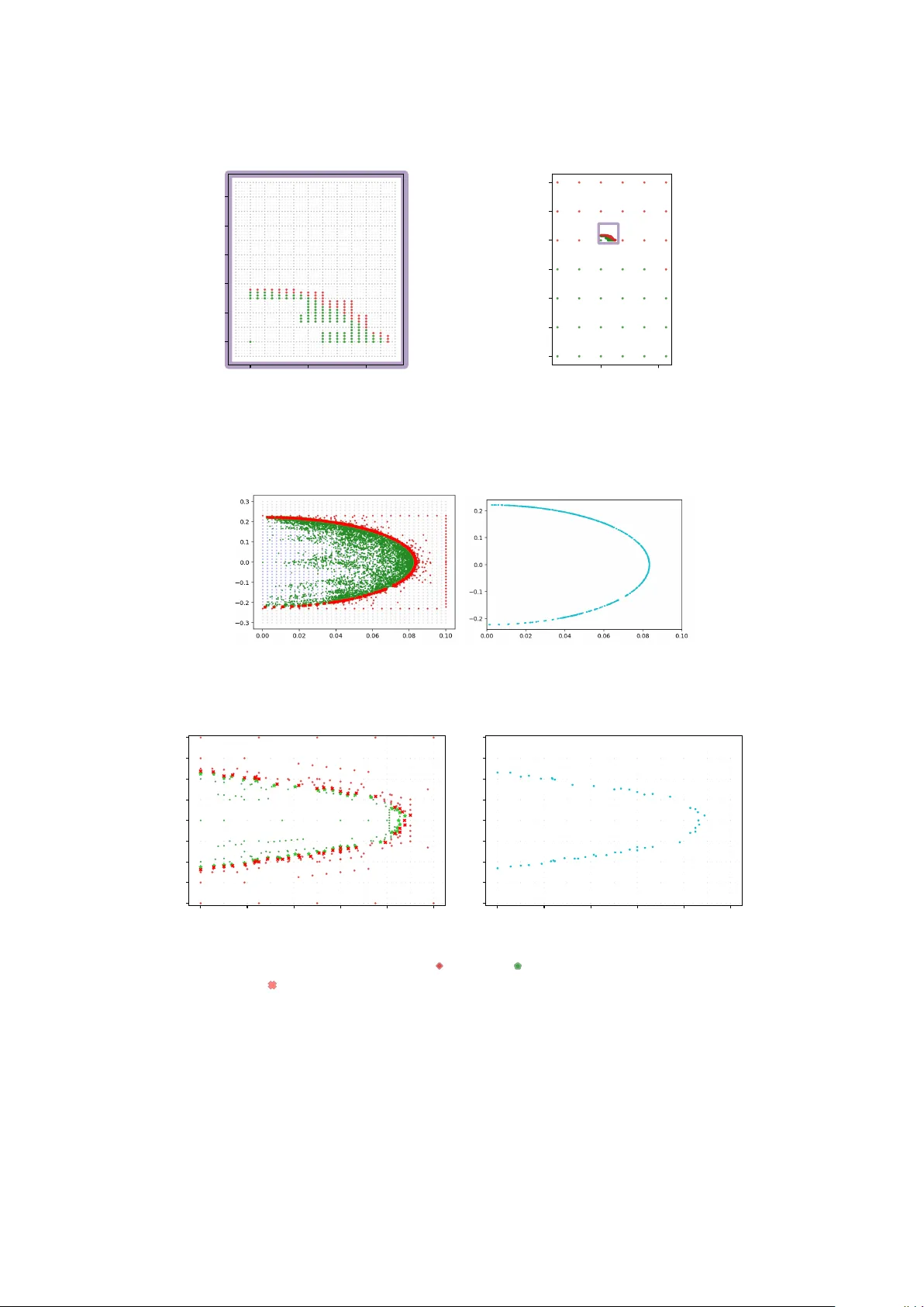
CRITICAL CUR VE OF TW O-MA TRIX MODELS AB B A , A { B , A } B AND AB AB , P AR T I: MONTE CARLO CARLOS I. PÉREZ SÁNCHEZ Abstra ct. F or a family of t wo-matrix models 1 2 T r( A 2 + B 2 ) − g 4 T r( A 4 + B 4 ) −      h 2 T r( AB AB ) h 4 T r( AB AB + AB B A ) h 2 T r( AB B A ) with hermitian A and B , we provide, in each case, a Monte Carlo estimate of the b ound- ary of the maximal con vergence domain in the ( h, g ) -plane. The results are discussed comparing with exact solutions (in agreement with the only analytically solved case) and phase diagrams obtained b y means of the functional renormalisation group. Figure 1. Sketc h of the phase diagram of three mo dels. The top left plot lies inside the three dark ened regions of each of the three other plots. 1. Intr oduction W e determine the critical lo ci of a family of in tegrals o v er tw o hermitian random ma- trices, A and B , of a large size N . F or q ∈ [0 , 1] , g , h ∈ R , let S ( q ) g ,h ( A, B ) = 1 2 T r( A 2 + B 2 ) − g 4 T r( A 4 + B 4 ) − h 2 T r( A { B , A } q B ) (1.1) with the following notation { B , A } q := q B A + (1 − q ) AB , with 0 ≤ q ≤ 1 . (1.2) It is part of our presen t w ork to numerically determine the maximal real domains of the couplings g and h for which the partition function Z ( q ) N ( g , h ) = Z e − N S ( q ) g,h ( A,B ) d A d B (1.3) 1 2 C. I. PÉREZ SÁNCHEZ exists in the cases q = 0 , 1 2 and 1 . (The integration for eac h matrix is p erformed o v er its N 2 real degrees of freedom and the measure is so normalised, that at g = h = 0 the partition function is 1 , see Eq. ( 2.2 ) for details.) Setting q = 1 giv es rise to the AB AB -mo del (w e will name mo dels using essentially the op erator accompanying h ), which was analytically solv ed b y Kazak o v–Zinn-Justin (Jr.) in [ KZ-J99 ]. The AB AB -mo del is special, for one b ecause T r AB AB is not a p ositiv e-definite operator (this, as we will see, makes the phase diagram non-trivial) that, unlike T r A 3 , do es mix the matrices. But the AB AB -mo del is also imp ortant b ecause it was solv ed by the character expansion of [ KSW96 ], which pro v ed fruitful to others (e.g. [ BH09 ]) and do es so ev en at presen t [ APT25 ]. Unlik e one-matrix models, tw o-matrix models can b e solv ed only in exceptional cases. The full solution of one-matrix mo dels w as streamlined by Eynard-Orantin in their top o- logical recursion [ EO07 ] (if needed, to gain familiarity , see [ Eyn16 , Bor17 ] b efore); a family of tw o-matrix mo dels can b e solved by the same to ol [ Eyn16 , Ch. 8], but for an arbitrary p oten tial a general analytic to ol is not a v ailable. This happens with the models ( 1.1 ). It w ould b e interesting to study these using top ological recursion or the c haracter expan- sion 1 , but for the time b eing w e resort to computer simulations. Indeed, when h = 0 , the p oten tial do es no longer mix A with B and the tw o-matrix mo del will factor as Z ( q ) N ( g , 0) = [ z N ( g )] 2 , where z N ( g ) = R e − N T r M 2 / 2+ N g T r M 4 / 4 d M . This mo del is critical at g = +1 / 12 in the present sign conv en tion. Thus, for eac h q in ( 1.3 ), the critical p oin t ( g , h ) = (1 / 12 , 0) of pure gra vit y lies on the critic al curve , the b oundary of the maximal region on the ( g , h ) -plane where the mo del exist. Our Monte Carlo simulations find such critical curve and the asymptotics for large | h | . The first coarse conjecture—after a small excursion to the q = 3 4 -mo del that supp orts it—is that, in that limit , Mo dels ( 1.1 ) come in t w o fla v ours: q = 0 q = 1 2 q = 3 4 all ‘the same’ in teresting q = 1 (1.4) When q = 1 , the h -op erator T r AB AB is oscillatory , as it is non-trivially in tegrated under the U ( N ) -relative angle b et w een the tw o matrices that is presen t in ( 1.3 ); on the other end, T r AB B A = T r[ AB ( AB ) ∗ ] is constant under unitary in tegration. The exp ectation of the T r AB AB op erator is seen (n umerically , see Fig. 17 ) to tak e the sign of h , so the pro duct h T r AB AB has alw a ys the same sign in exp ectation, regardless of h (if g allo ws for finiteness). The U ( N ) -relative angle b ecomes then dominated b y a p ositive part inside the h -operator from q = 1 2 , yielding ‘the same’ asympotics in q ∈ [0 , 1 2 ] . It is p ertinen t to men tion that Mon te Carlo is only a c hoice to approac h this problem. Other n umerical techniques emerged more recently in the con text of lattice Y ang-Mills theory in [ AK17 ], who built a matrix of momen ts (that is essen tially indexed by lo ops in the lattice, and satisfies the T o epliz prop erty) and pro v ed that this matrix should be p ositiv ely defined. P ositiv e conditions hav e b een also notably employ ed in [ Lin20 ] for matrix mo dels of sev eral hermitian v ariables. In b oth cases, the en tries of the matrix 1 The character expansion is very unlikely to help here, since in the Kazak o v–Zinn-Justin solution of the AB AB -mo del, that metho d relied on the companion op erator of h b eing (the trace of ) an analytic function F ( z ) = z 2 of AB ; for q < 1 , the analogue function F q ( z ) = q z 2 + (1 − q ) | z | 2 dep ends on the conjugate of z . CRITICAL CUR VE OF q -DEFORMED TW O-MA TRIX MODELS, P AR T I 3 of moments can b e computed recursiv ely , using lo op or Sc hwinger-Dy son equations, in terms of a finite family of momen ts. The p ositivit y b ounds yield a parametrisation of all momen ts in terms of the coupling constants, whic h b eing so sharp (see in particular [ KZh22 ]), effectiv ely yields a solution of the mo del, the cut off being now no longer the size of the random matrices but that of the matrix of moments. In eac h case, the proof of p ositivit y is itself trivial, but its consequences are p o w erful and seemingly enjoy of a univ ersal applicabilit y [ Lin20 , HKP22 , Pér25 , BH24 , KM25 , KPPS20 , L T26 , PPS26 ]. In the case at hand, ev en though it should b e p ossible to ‘b o otstrap’ the mo dels ( 1.1 ) for all q inside a single program using this approach, it is adv an tageous to hav e Monte Carlo sim ulations ready as an indep endent metho d to con trast with. Part II of this pap er series addresses the viewp oint of criticalit y b y using p ositivity conditions for biv ariate matrix mo dels lik e ( 1.1 ). Other metho d to estimate the critical lo ci of multi-matrix mo dels is the functional renormalisation group whic h seems effectiv e for a first exploration, as it requires less resources than Monte Carlo and deliver a prompt, in case of random matrices, qualita- tiv e answer. In the case of m ulti-matrix mo dels, this approach is still in the pro cess of telling apart criticalit y for differen t mo dels: in fact, by zo oming out the ‘phase diagram of the AB AB -mo del’ that was deriv ed in [ EPP20 ] one observ es the lac k of the symmetry h 7→ − h commented under ( 1.4 ) and one disco v ers an asymptotic b eha vior that, thanks to the presen t sim ulations, can b e identified as characteristic of a q -mo del with q ≤ 1 2 (cf. Sec. 5.1 to see why this paragraph is in part also self-critique). The co de [ Pér26 , DOI DOI 10.5281/zenodo .19236121 10.5281/zenodo .19236121 ] that w e designed to perform the exp erimen ts of the presen t article should immediately w ork for other biv ariate tw o-matrix mo dels, and after an ob vious extension, for an y m ulti-matrix mo del. Commencing with the relev an t metho ds for multi-matrix mo dels in Section 2 , we then briefly explain the Hamiltonian Mon te Carlo (MC) approach in Section 3 . Our co de was benefited from the op enness of the co de of [ Jha22 ] 2 . W e mo dified part of it to matc h our needs and extended it by new metho ds to find the critical curve. Our implemen tation is describ ed in Section 4 . Then Section 5 presents the results and Section 6 closes with the persp ective and conclusions. T o finish, we remark that all plots b efore Section 5 are actual sim ulations, but w ere added only for exp osition and notation purposes. Ho w ever, only the plots of Section 5 w ere taken in to accoun t in the final statistics. Contents 1. In tro duction 1 2. T wo-matrix mo dels 4 2.1. P ositivit y 4 2.2. Sc h winger-Dyson Equations 5 3. Hamiltonian Mark o v Chain Mon te Carlo 7 3.1. Generation of new prop osals 7 3.2. Up date rules 10 4. New, dynamic metho ds in th e Python co de 10 4.1. Midp oin t searc h 12 2 This reference provides a co de written in Python ; for C++ co de, we refer to e.g. [ BG16 , D’A22 ] who addressed a related problem, if with more structure (and rather using Metrop olis-Hastings Monte Carlo). 4 C. I. PÉREZ SÁNCHEZ 4.2. Radial searc h 12 4.3. Angular searc h 12 4.4. Sc h winger-Dyson equations and thermalisation 13 5. Results 14 5.1. Bon us: On m ultimatrix functional renormalisation 16 6. Conclusions 17 App endix A. F urther impro v emen ts in the algorithm 19 App endix B. Notation 21 References 22 2. Tw o-ma trix models Let us denote by H N the space of N × N (complex) hermitian matrices. W e compute the correlators or exp ectation v alues of wor ds W A,B in tw o letters (monomials W A,B ∈ C ⟨ A, B ⟩ lik e A 4 B AB ) by E [ 1 N T r( W A,B )] = 1 Z Z H N × H N 1 N T r( W A,B )e − N S ( A,B ) d A d B . (2.1) Of course, we should write E ( q ) g ,h ; N , Z ( q ) N ( g , h ) and S ( q ) g ,h instead of E , Z and S , but we use this heavier notation only if the con text is not clear. In Eq. ( 2.1 ) the measure is giv en b y d M = 2 − N/ 2 ( N /π ) N 2 / 2 N Y i =1 d M ii Y j = i +1 ,...,N d Re M ij d Im M ij ( M = A, B ) (2.2) whic h yields d A d B normalised in the sense that Z (0 , 0) = 1 , and Eq. ( 2.1 ) yielding 1 for the empt y word W A,B = 1 N (this also fixes notation for the trace). 2.1. P ositivit y. F or a fixed matrix mo del (fix q ), since P N a,b =1 M a,b ¯ M a,b > 0 holds for an y matrix M ∈ M N ( C ) so do es for an y complex linear com bination M = P L i =1 z i W i of arbitrarily many ( 0 < L < ∞ ) w ords W i ∈ C ⟨ A, B ⟩ in the letters A and B , z i ∈ C . Thus 0 < L X i,j =1 z i T r( W i W ∗ j ) ¯ z j , hence 0 < L X i,j =1 z i E [T r( W i W ∗ j )] ¯ z j (2.3) for ev ery z = ( z i ) ∈ C L . The latter implies the non-negativit y of the matrix M , M ⪰ 0 with en tries M ij := lim N →∞ 1 N E [T r W i W ∗ j ] = M j i . (2.4) By restoring the notation, one sees that M of course dep ends on g and h and M ( g , h ) ⪰ 0 restricts the domain of ( g , h ) . W e are already in the large- N regime, so the N -dep endence disapp eared; in the large- L limit one gets the solution of the mo del in the sense of having determined all correlators { E [ W ] : W ∈ C ⟨ A, B ⟩ , deg W ≤ L } (2.5) as a n umerical estimate in terms of each ( g , h ) , th us also the maximally allow ed domain. The sufficiency of a suitable set of indep endent parametrising momen ts —despite the exp onen tially gro wing family—has b een addressed by [ Lin20 ]. CRITICAL CUR VE OF q -DEFORMED TW O-MA TRIX MODELS, P AR T I 5 Although simple, tw o inequalities will be useful: − T r AB B A ≤ T r AB AB ≤ T r AB B A and (2.6a) T r AB B A ≤ 1 2 T r( A 4 + B 4 ) . (2.6b) The first hierarc h y of op erators can b e obtained (in particular) by using Ineqs. ( 2.3 ) with M = z 1 W 1 + z 2 W 2 ; then th e matrix T r( W i W ∗ j ) is non-negative, hence det[(T r W i W ∗ j ) i,j ] ≥ 0 which is equiv alen t to Ineq. ( 2.6a ), when W 1 = AB , W 2 = B A . The second one rephrases the trivial fact that 0 ≤ T r C ∗ C for any square matrix C , and esp ecially when C = A 2 − B 2 . F rom Ineq. ( 2.6a ), which is still deterministic, observe that for fixed couplings ( g , h ) and matrices A, B ∈ H N , the function q 7→ S ( q ) g ,h ( A, B ) is non-decreasing in the parameter q , hence the in tegrand in Eq. ( 1.3 ) is non-increasing with q : e − N S (0) g,h ( A,B ) ≥ e − N S ( q ) g,h ( A,B ) ≥ e − N S ( ˜ q ) g,h ( A,B ) ≥ e − N S (1) g,h ( A,B ) , ( g , h ) ∈ R 2 ≥ 0 , q < ˜ q . (2.7) F or fixed g > 0 , if there exist a p oin t ( g , h q ( g )) in the critical curv e of the q -mo del, the previous inequality means that if ( g , h ˜ q ( g )) is in the critical curve of the ˜ q -mo del, then h ˜ q ( g ) ≥ h q ( g ) . Restricting ourselves temporarily to R 2 ≥ 0 , we conclude that no p oint of the segmen t of the critical curve for the q -mo del in that p ositive quadrant can lie outside the con v ergen t region of the ˜ q -mo del, if q < ˜ q ≤ 1 . After Section 4 , it will b e clear, that one sa v es also cpu -time b y starting with the AB AB -mo del, determining its critical curve, and use this information to simulate for mo dels with q < 1 . In the In tro duction we commen ted on the b ound g ≤ 1 / 12 (when h = 0 ) required for the mo dels to exist. Again b y ( 2.6a ), if q ∈ [0 , 1 2 ] then T r A { B , A } q B ≥ 0 , hence also for h > 0 one obtains the b ound g ≤ 1 / 12 . Now we refer to the exact solutions when g = 0 , whic h yield a critical h v alue giv en by h q =1 ( g = 0) = 2 / 9 [ CK96 , Sec. 5.3, in terms of the inv erse coupling or temp erature, T ∗ = 4 . 5 ] or [ KZ-J99 , App. A] for the AB AB -mo del ( q = 1 -case). But then Bounds ( 2.7 ) imply that h q ′ ( g = 0) ≤ h q =1 ( g = 0) = 2 / 9 for an y q ′ ≤ 1 . (2.8) Hence, the segment in R 2 ≥ 0 of the critical curv e lies in the rectangle [0 , 1 / 12] × [0 , 2 / 9] for q ∈ [0 , 1 2 ] and Ineq. ( 2.8 ) holds for any q . (This is ho w ev er what w e kno w b efore sim ulations. After these, one observ es that also for q = 1 it holds that g ≤ 1 / 12 whenev er h > 0 , since, for an y h , E ( q =1) g ,h [T r AB AB ] tak es the same sign of h , see Fig. 17 .) P ositivit y is also men tioned b ecause its application to solve path in tegrals in general is relativ ely new. F or instance, few is known ab out the precise v alue of determinants of (the minors of ) M . Our Python program monitors this. In order to compute the en tries of M , the loop or Sc h winger-Dyson equations, whic h w e address b elow, are used. 2.2. Sc h winger-Dyson Equations. While it is p ossible to geometrically describ e the origin of the Sc hwinger-Dyson Equations (cf. [ AK24 ]), w e here pro vide the shortest deriv ation and fo cus on them as a to ol. Giv en tw o w ords X ( A, B ) , Y ( A, B ) in the tw o matrix v ariables A, B , the field F = ( X , Y ) : H N × H N → H N × H N is smo oth. F rom 6 C. I. PÉREZ SÁNCHEZ R d( F e − N S ) = 0 it follo ws Z (div F )e − N S = N Z X α =1 ,..., 2 N 2  F α ∂ α S e − N S  d A d B (2.9) up on identification of d with the divergence, as it acts on the v ector field F : R 2 × N × N → R 2 × N × N . Op erationally , it is conv enien t to pass from 2 N 2 real v ariables to equiv alen t ‘co ordinate’ free definitions that allo w to compute only by mo ving letters, [ Gui16 , Pér21 ]. This is not only an adv antage to obtain compact expressions for the Sch winger-Dyson Equations but the co de profits from these to o wh ile computing the force that leapfrog in tegration needs (cf. Sec. 3.1 ). The first half of v alues for α corresp ond to ( ∂ A ) i,j and the other to ( ∂ B ) i,j for i, j = 1 , . . . , N , so one obtains E [div F ] = N E [T r( X ∂ A S + Y ∂ B S )] ; here the expression X ∂ A S means matrix multiplication of X with ∂ A S . In order to obtain the matrix deriv ativ e ∂ A , one defines for M k ∈ M N ( C ) and A ∈ H N , D A ( M 1 M 2 · · · M p ) := ∂ A T r( M 1 M 2 · · · M p ) (2.10) := X i =1 ,...,p if M i = A M i +1 M i +2 · · · M p M 1 · · · M i − 1 . The op erator D A is called cyclic gradient [ V oi00 ]; notice that D A W is indep endent of the cyclic reo drerings of W (and b eing the deriv ativ e of a trace, it must b e). Finally , the div ergence of F = ( X , Y ) is giv en by div F = ∂ A X + ∂ B Y . In order to make sense of this expression one uses the matrix deriv ativ es (or noncommutativ e deriv ativ es), which are defined by (here δ M k ,A = 1 only if M k = A , and else δ M k ,A = 0 , and notice the absence of the trace in the argument) ∂ A ( M 1 M 2 · · · M p ) := δ M 1 ,A 1 ⊗ M 2 . . . M p (2.11) + X 1 log 1 /p , whereas the R 2 ( ˜ p ) is ver- ified in the case of the prop osed mo ve for the purple p oints, as the b ound (1 / N ) log(1 / ˜ p ) was not exceeded ( p, ˜ p are freshly uniformly chosen random num bers in (0 , 1) for each acceptance test). B A P B P A ϵf t f t = − N ∇ S ( X t ) P t +1 / 2 P t − 1 / 2 X t X t +1 ϵP t +1 / 2 P 1 / 2 · · · (random) Figure 3. On the Hamiltonian approac h to MCMC with the leapfrog in tegrator. The left (righ t) plane is the ‘configura- tion’ (resp. momen ta) H 2 N -space of matrices X t = ( A t , B t ) [resp. P t +1 / 2 = ( P A,t +1 / 2 , P B ,t +1 / 2 ) ]. The gradien t’s components are matrix deriv ativ es 4 defined in Eq. ( 2.11 ). F or the p oten tial S = S ( q ) g ,h ( A, B ) in Eq. ( 1.1 ), the force f = ( f A , f B ) is given by 1 N f A = A − g A 3 − hq B AB − 1 2 h (1 − q )( B B A + AB B ) (3.5a) 1 N f B = B − g B 3 − hq AB A − 1 2 h (1 − q )( AAB + B AA ) (3.5b) The time is discretized with a small step-size ϵ (in the co de ϵ = 10 − 4 for all sim ulations; faster choices migh t b e p ossible, but one nev er should c hange this parameter for a set of sim ulations). Then momenta are iterated at half-time units, starting with a fresh, randomly chosen P 1 / 2 ∈ H 2 N . The momentum P t +1 / 2 for t = 1 , 2 , . . . , ⌊ T /ϵ ⌋ is obtained from the previous one b y letting the force act during time interv al ϵ , P t +1 / 2 = P t − 1 / 2 + ϵf ( A t , B t ) = P t − 1 / 2 − ϵN ∇ X S ( A t , B t ) (3.6a) while the matrices X t +1 = ( A t +1 , B t +1 ) are generated b y integrating the momen tum P t +1 / 2 = ( P A , P B ) t +1 / 2 b et w een time t and t + 1 , X t +1 = X t + ϵP t +1 / 2 (3.6b) This is illustrated in Figure 3 . Then let ˜ X = X ⌊ T /ϵ ⌋ and accept or reject according to the rules of Section 3.2 . 4 The ( ij ) entry of a matrix deriv ative is ∂ /∂ M j i , which often app ears as ∂ M = ∂ /∂ M T ; w e refer to [ Pér21 ] for more details, since pro vide only the expressions needed in the co de 10 C. I. PÉREZ SÁNCHEZ 3.2. Up date rules. First, assume that w e w an t to generate, given a mem b er X i ∈ H 2 N of the Mark ov Chain already , the next element X i +1 . T o this end one prop oses ˜ X ∈ H 2 N (Sec. 3.1 told ho w to prop ose ˜ X ). • F or a candidate ˜ X : If S ( ˜ X ) − S ( X i ) < 0 , then accept ˜ X =: X i +1 ( R 1 ) • Pick p uniformly distributed from (0 , 1) . If 0 < S ( ˜ X ) − S ( X i ) < 1 N log 1 p , then accept ˜ X =: X i +1 ( R 2 ( p ) ) (This, in particular, requires R 1 to be false.) • If b oth failed, let X i +1 = X i and propose another candidate. Figure 2 sketc hes the previous rules. The first one tends to sp end time at the first lo cal minim um, so without R 2 ( p ) the simulation would remain there. One th us allows new configurations to clim b the p oten tial but only as far as the increment do es not exceed N − 1 log(1 /p ) > 0 . 4. New, d ynamic methods in the Python code Let us denote by MC ( g , h ) the bo olean function, whose output is decided by con v er- gence ( True ) or div ergence ( False ) after p erforming MCMC on the p oin t ( g , h ) ∈ R 2 . Although this function dep ends of course of the matrix size and the iteration num ber n , these parameters are k ept fixed for eac h set of sim ulations, and w e simplify the notation. By definition, a simulation yields MC ( g , h ) = False if an y expectation v alues div erges at a Mark o v Chain length i < n , i.e. after i iterations or if the hermiticity of the proposed Mark o v Chain members is irrev ersibly 5 lost at i < n . In that case the phase diagram marks the p oin t ( g , h ) with the symbol . If all exp ectation v alues con verge and hermitic- it y is kept during the n iterations, then MC ( g, h ) = True and ( g , h ) is a denoted b y . W e designed the next routines to dynamically find pairs of opp osite truth v alue that are close enough. This is needed, since a naiv e strategy based on testing a ‘static’ set (e.g. a lattice) is helpful only initially , in order to obtain a glimpse of the phase space structure. How ev er, for more serious exp eriments a fixed discrete set turns out to be to o exp ensiv e. As a matter of fact, we started the simulations only on a region slightly bigger than that in Figure 4a . F or this, one can run the script of [ Jha22 ] in a double lo op; then it w as clear, that a dynamical extension of that co de w as needed to find the critical curve. Later w e will be able to explain in whic h sense to test a point for criticalit y is a particularly expensive Mon te Carlo integration. This imp oses constrain ts on the n um b er of p oints to b e tested. This section explains the strategies used to thriftily test p oints, instead of p erforming a test lik e in Figure 5a . No w fix a δ > 0 . W e shall lo ok for dip oles , i.e. t w o p oin ts ( g , h ) and ( g ′ , h ′ ) of different truth v alue that are at a distance δ in the R 2 plane. When suc h a dip ole is found, 1 2 ( g + g ′ , h + h ′ ) is added to the critical curve and we emplo y a sp ecial notation: ⋆ and instead of and , resp ectiv ely . 5 This means, that after certain fixed num b er of consecutiv e attempts to make a Mark ov Chain member hermitian failed. CRITICAL CUR VE OF q -DEFORMED TW O-MA TRIX MODELS, P AR T I 11 0 . 0 0 . 1 0 . 2 h 0 . 00 0 . 05 0 . 10 0 . 15 0 . 20 0 . 25 g Phase diagram: ABAB -mo del, with N = 150 and 1500 iterations (a) 0 1 h − 2 . 0 − 1 . 5 − 1 . 0 − 0 . 5 0 . 0 0 . 5 1 . 0 g Phase diagram: ABAB -mo del, with N = 150 and 1500 iterations (b) Figure 4. A naiv e test of lattice p oin ts is not efficient. This leads to dynamical metho ds to search the boundary of the conv ergen t region, see in Sec. 4 . (a) T esting a large num ber of p oints with a dummy (the characteristic function on an ellipse) to illustrate the midp oin t division strategy . One started here with the outer False -rectangle and a few True -p oin ts around the origin. 0 . 00 0 . 02 0 . 04 0 . 06 0 . 08 0 . 10 g − 0 . 4 − 0 . 3 − 0 . 2 − 0 . 1 0 . 0 0 . 1 0 . 2 0 . 3 0 . 4 h Phase space ABAB -mo del, with N = 150 and 1500 iterations 0 . 00 0 . 02 0 . 04 0 . 06 0 . 08 0 . 10 g − 0 . 4 − 0 . 3 − 0 . 2 − 0 . 1 0 . 0 0 . 1 0 . 2 0 . 3 0 . 4 h Critical curve, AB AB -model, with N = 150 and 1500 iterations (b) The cpu -time for MC ( g , h ) is ≈ 400 secs., with N = 150 and n = 1500 . F or this small num ber of interactions n , and each tak e ab out the same time, and a dip ole ( ⋆ , ) tak es usually at least half an hour. (This iteration n um b er is not enough to see criticalit y , and this plot is presented merely with didactic purposes; mind the axis in version too.) Figure 5. ‘Exp ectation (a) vs. realit y (b)’. In (a), instead of MC w e use as dumm y a c haracteristic function. When p oin ts of opp osite truth v alue lie a fixed distance δ apart (a ‘dip ole’) their middle p oint is added to the critical curve. 12 C. I. PÉREZ SÁNCHEZ 4.1. Midp oin t searc h. Another v ery simple, but initially useful routine is to use a midp oin t searc h. Start with a pair of p oin ts P 0 = ( g 0 , h 0 ) , Q 0 = ( g ′ 0 , h ′ 0 ) ∈ R 2 of dif- feren t truth v alue — w.l.o.g. MC ( P 0 ) = True . Supp ose that ( P i , Q i ) ∈ R 2 × R 2 with MC ( P i ) = True , MC ( Q i ) = False for some integer i > 0 w ere found. If the distance b et w een P i and Q i is less than δ , w e are done and ( P i , Q i ) = ( ⋆ , ) . Else one lets ( P i +1 , Q i +1 ) := (  P i + Q i 2 , Q i  if MC ( P i + Q i 2 ) = True  P i , P i + Q i 2  if MC ( P i + Q i 2 ) = False (4.1) whic h b y construction is a pair of points of opp osite truth v alue (Fig. 6 ). The algorithm con v erges to a dip ole, at the latest after m steps, if 2 m > (1 /δ ) p ( g 0 − g ′ 0 ) 2 + ( h 0 − h ′ 0 ) 2 . Figure 6. Picturing Algorithm ( 4.1 ) with a simulation at N = 150 , n = 1500 at h = 0 (hence v alid for all q -mo dels) starting from the (green) origin and red p oin t (0 , 1 / 10) . 4.2. Radial searc h. Our Python-co de will abandon the ev aluation of MC ( g , h ) in case of finding div ergen t quantities or too man y failed attempts to mak e matrices hermitian, and prop oses the next p oint to b e ev aluated b y MC . While lo oking at dip oles, it sa ves resources to mo v e from p otential red p oints, ev aluate these, and if the result is False , to mo v e to w ards the origin at a step δ > 0 in radial direction, i.e. testing MC ( g − δ g / p g 2 + h 2 , h − δ h/ p g 2 + h 2 ) (4.2) One contin ues the pro cess un til a green p oint is found, whic h must happ en since w e mov e to w ards the origin (ho wev er, the co de is taking care that one do es not unluc kily exceeded a maximum of steps; this is tragic, if the initial guess is to o far). Since the last red p oin t and the new first green p oin t are at a distance δ , we obtain a dip ole and add it to the critical curve. The flow diagram for this part of the Python script is depicted in Figure 9 . During our exp eriments we realised that one can sa v e resources by making δ dep en- den t on the num ber of iterations at which the previous p oin t div erged. F or instance, if Python abandons the calculation of MC ( g , h ) to o so on (say ab out n/ 10 iterations), w e w aste resources b y adv ancing only a step δ . On the other hand, if MC ( g , h ) div erged just b efore the planned n iterations, this means that the green p oint is lik ely near, and we lo ose information b y taking the whole step δ . This sa v es time and w as implemen ted (see App. A for this impro v emen t) but since it complicates the final statistics, so w e stuck to a uniform δ = 0 . 0015 step to find dip oles in the quadrant R ≥ 0 × R ≥ 0 , and else we used an angular searc h describ ed next. 4.3. Angular searc h. Sp ecially to determine the asymp otics of each critical curv e, a complemen tary metho d that tests p oints along a circumference arc is helpful. F or this, it is again to o exp ensiv e to stick to our dip ole definition in the sense of spatial separation, and we need a surrogate (keeping the same notation here and in the plots) for angular separation α . F or θ ∈ [0 , 2 π ] , let Rot θ ( g , h ) = (cos θ · g − sin θ · h, sin θ · g + cos θ · h ) b e the p oin t ( g , h ) rotated b y the angle θ . Starting with a non-zero red p oint Q 0 = ( g , h ) ∈ R 2 − { 0 } , one lets Q k +1 = Rot kα ( g , h ) for k ∈ Z ≥ 0 if MC ( Q k ) = False . Else, w e found our ‘angular’ CRITICAL CUR VE OF q -DEFORMED TW O-MA TRIX MODELS, P AR T I 13 0 . 00 0 . 02 0 . 04 0 . 06 0 . 08 0 . 10 0 . 12 0 . 14 0 . 16 h 0 . 00 0 . 02 0 . 04 0 . 06 0 . 08 0 . 10 g Phase diagram: AB B A -model, with N = 150 and 2200 iterations Figure 7. R adial se ar ch. Starting from p oten tially red p oin ts, one adv ances a distance δ (here dep ending on how so on MC div erged at the previous p oint, in the sense of App. A ) tow ards the origin un- til a p oin t along a the same ray yields for MC a True . The couple of this conv ergen t p oin t and the last div ergent p oin t are a dip ole denoted b y a green star and a red cross. − 20 − 15 − 10 − 5 0 5 10 15 20 h − 20 − 15 − 10 − 5 0 g Phase diagram: AB AB -mo del with N = 32 and 20000 iterations Figure 8. Angular se ar ch. Starting from green p oints, one consecutiv ely tests p oin ts on a circumference cen tered at (0 , 0) until a divergen t p oint is found. This is expensive, e.g. one of the long tails in the zoomed region took O (10 4 ) secs. ( ≈ 3 hrs.) to find the respective dip ole. A faster, negated v ersion w as also implemen ted (see the red p oin ts with de- creasing | h | ). dip ole, and we draw ⋆ for Q k and for Q k − 1 on the phase diagram. An actual p oin t (out of tw o) of the critical curve at radius p g 2 + h 2 m ust be in the arc segmen t spanned by these t w o p oints (and the other very far). In particular, since the eigen v alue distribution stresses for large v alues of −| g | and −| h | , it is con v enient not to only trust the previous searc h for green p oints. Instead, to b e sure that w e find an arc where the critical curve should pass through, we implemen ted the ‘negated’ v ersion of the previous pro cess. Namely , start with a green p oint now, P 0 = ( g , h ) ∈ R 2 − { 0 } . Then let P k +1 = Rot kα ( g , h ) for k ∈ Z ≥ 0 if MC ( P k ) = True , while if MC ( P k ) = False then ( ⋆ , ) = ( P k − 1 , P k ) is a dip ole. F or large n , we stress that c hasing a red point starting with green p oin ts tak es m uc h longer than c hasing green p oints starting from a red ones, since we imp osed that Python ab orts of the calculation so on after first clear signs of div ergence; since plots are generated also when divergences happ ened, w e can b e sure that we did not ab ort the calculation to o so on (see Fig. 8 ). Another cpu -time economy asp ect is the following: w e did not k eep this angular separation constant, so the maximum of all angular steps is the one that con tributes to the discretisation part of the error bars. 4.4. Sc h winger-Dyson equations and thermalisation. It ob vious that the thermali- sation sp eed increases with the matrix size (see Fig. 10 ), but less so is to determine when, for fixed N , thermalisation tak es place. Our Python code monitors the Sc h winger-Dyson equations during each run. Eac h word in A, B or (noncommutativ e monomial) defines according to Section ( 2.2 ) a matrix field, whose resp ective Sch winger-Dyson equations are listed in T able 1 . F or a fixed w ord W A,B , the random v ariable ‘left hand side (LHS) min us righ t hand side (RHS)’ of the SDE for W A,B is sav ed and prin ted as output, as in Figure 11 . F or future w orks, this feature can be used as a clearer criterion for determining the thermalisation time τ of Section 3 . The rationale is the follo wing: whereas it is hard to 14 C. I. PÉREZ SÁNCHEZ MC ( g , h ) Finite E ’s, m atrices k eep True False hermiticit y , health y e.v. distribution Prin t 0 2500 5000 7500 10000 12500 15000 17500 20000 Time units 0 . 0 0 . 2 0 . 4 0 . 6 0 . 8 1 . 0 MC for ( A 2 + B 2 ) / 2 − ( g / 4)( A 4 + B 4 ) − ( h/ 2) AB AB , A, B of size N = 32 tr A tr B t 2 , all at g = − 0 . 0625 , h = 0 . 3078 0 2500 5000 7500 10000 12500 15000 17500 20000 Time units 0 . 0 0 . 5 1 . 0 1 . 5 2 . 0 AB AB -mo del , ( g , h ) = ( − 0 . 0625 , 0 . 3078), A, B of size N = 32 t 4 t 2 , 2 t 1 , 1 , 1 , 1 − 0 . 06 − 0 . 04 − 0 . 02 0 . 00 0 . 02 0 . 04 0 . 06 λ (normalized b y 1 / N ) 0 500 1000 1500 2000 2500 3000 ρ ( λ ) Eigen v alues: AB AB -mo del , N = 32 , ( g , h ) = ( − 0 . 06247 , 0 . 30781) Eig( A ) Eig( B ) . . . 0 2500 5000 7500 10000 12500 15000 17500 20000 Time units 0 5 10 15 20 25 30 MC for ( A 2 + B 2 ) / 2 − ( g / 4)( A 4 + B 4 ) − ( h/ 2) AB B A , A, B of size N = 32 tr A tr B t 2 , all at g = − 71 . 1628 , h = 72 . 2744 0 2500 5000 7500 10000 12500 15000 17500 20000 Time units 0 1000 2000 3000 4000 5000 6000 7000 8000 AB B A -mo del , ( g , h ) = ( − 71 . 1628 , 72 . 2744), A, B of size N = 32 t 4 t 2 , 2 t 1 , 1 , 1 , 1 − 0 . 6 − 0 . 4 − 0 . 2 0 . 0 0 . 2 0 . 4 0 . 6 λ (normalized b y 1 / N ) 0 10000 20000 30000 40000 50000 ρ ( λ ) Eigen v alues: AB B A -mo del , N = 32 , ( g , h ) = ( − 71 . 16276 , 72 . 27438) Eig( A ) Eig( B ) . . . Prin t Add a green star at ( g , h ) and mo v e to a p oin t with a differen t angle ↶ ? Add a red p oin t at ( g , h ) and mo v e radialy redefing ( g , h ) as ← ( g − δ g / p g 2 + h 2 , h − δ h/ p g 2 + h 2 ) (a) Radial searc h flow diagram. MC ( g , h ) Finite E ’s, m atrices k eep True False hermiticit y , health y e.v. distribution Prin t 0 2500 5000 7500 10000 12500 15000 17500 20000 Time units 0 . 0 0 . 2 0 . 4 0 . 6 0 . 8 1 . 0 1 . 2 1 . 4 A { B , A } B -mo del , ( g , h ) = ( − 0 . 4993 , 0 . 7654), A, B of size N = 32 t 4 t 2 , 2 t 1 , 1 , 1 , 1 0 2500 5000 7500 10000 12500 15000 17500 20000 Time units − 0 . 2 0 . 0 0 . 2 0 . 4 0 . 6 0 . 8 1 . 0 1 . 2 LHS − RHS on eac h SDE A (v arying A ) B (v arying B ) A 3 (v arying A ) B 2 A (v arying A ) B AB (v arying A ) SDE in the A { B , A } B -mo del; N = 32 and 20000 times, g = − 0 . 499 , h = 0 . 765 − 0 . 06 − 0 . 04 − 0 . 02 0 . 00 0 . 02 0 . 04 0 . 06 λ (normalized b y 1 / N ) 0 500 1000 1500 2000 2500 3000 ρ ( λ ) Eigen v alues: A { B , A } B -mo del , N = 32 , ( g , h ) = ( − 0 . 49933 , 0 . 76544) Eig( A ) Eig( B ) . . . 0 250 500 750 1000 1250 1500 1750 2000 Time units 0 . 00 0 . 25 0 . 50 0 . 75 1 . 00 1 . 25 1 . 50 1 . 75 MC for ( A 2 + B 2 ) / 2 − ( g / 4)( A 4 + B 4 ) − ( h/ 2) AB AB , A, B of size N = 50 tr A tr B t 2 , all at g = 0 . 0866 , h = 0 . 1347 0 250 500 750 1000 1250 1500 1750 2000 Time units − 0 . 2 0 . 0 0 . 2 0 . 4 0 . 6 0 . 8 1 . 0 1 . 2 LHS − RHS on eac h DSE A (v arying A ) B (v arying B ) A 3 (v arying A ) B 2 A (v arying A ) B AB (v arying A ) SDE in the AB AB -mo del; N = 50 and 2000 times, g = 0 . 087 , h = 0 . 135 0 250 500 750 1000 1250 1500 1750 2000 Time units 0 10 20 30 40 50 60 70 80 Determinan t of momen ta matrices M 0 M 1 M 2 M 3 M 4 M 5 M 6 M 7 P ositivit y: AB AB -mo del; N = 50, 2000 iterations, g = 0 . 087 , h = 0 . 135 . . . Prin t Add a green p en tagon at ( g , h ) and redefine ( g , h ) b y Add a red p oin t at ( g , h ) and c ho ose a new ( g , h ) with differen t radius ← (cos θ · g − sin θ · h, sin θ · g + cos θ · h ) (b) Flo w diagram of the angular search. Figure 9. Flo w diagrams for the tw o main searc h routines. In the case of (b), this is the searc h for divergen t p oints starting from a con vergen t p oin t (a negated v ersion is easily derived from this, by swapping True with False and green with red p oints). When the initial p oin ts are exhausted, part of the output is, in each case, a diagram lik e those in Figs. 7 and 8 . c ho ose a criterion to determine τ by the stabilization of t 2 , t 1 , 1 , 1 , 1 , t 2 , 2 , t 4 , . . . of Eqs. ( 2.13 ) — partially b ecause it is precisely MC’s aim to determine those v alues — it is m uc h easier to set a b ound ϵ > 0 and to determine τ b y lo oking at the mem bers { ( A i , B i ) } i =1 , 2 ,...,n of the Mark o v Chain and letting τ b e the first index i 0 ∈ { 1 , . . . , n } that verifies finite X W A,B  LHS-RHS of the SDE for W A,B  2     A i 0 ,B i 0 < ϵ. (4.3) 5. Resul ts After comparing several pairs ( N 1 , n 1 ) , ( N 2 , n 2 ) , . . . of matrix sizes N i and and iterations n i , w e c hose N = 32 (see Figs. 12 and 13 ) as N = 32 is the smallest v alue for which com- parison with analytically p erformed large- N matrix integration w ould yield corrections of the order of N − 2 ≲ 10 − 3 (corresp onding to toric and higher-gen us corrections N 2 − 2 g for g = 1 , 2 , . . . ). T o comp ensate this, and in order to ensure that w e detect criticality , our Mark o v c hains are quite long ( n = 2 × 10 4 ). A comparison concerning the stability with resp ect to matrix size is presented in Figure 14d . CRITICAL CUR VE OF q -DEFORMED TW O-MA TRIX MODELS, P AR T I 15 Figure 10. Thermalisation sp eed as function of N for the AB B A -mo del at a (con ver gent) p oint ( g , h ) = (0 . 05 , 0 . 05) . Figure 11. Thermalisation and the fail- ure for SDEs to hold. In the plot legend means the fiv e equations tested: ‘ W A,B (v arying A )’ means that the field X = W A,B , Y = 0 , while ‘ W A,B (v arying B )’ means Y = W A,B , X = 0 in T able 1 . 0 1000 2000 3000 4000 5000 6000 Time units − 0 . 5 0 . 0 0 . 5 1 . 0 1 . 5 2 . 0 MC for ( A 2 + B 2 ) / 2 − ( g / 4)( A 4 + B 4 ) − ( h/ 2) AB AB , ( g , h ) = (0 . 084 , 0 . 001) t 2 at N = 45 t 2 at N = 55 t 2 at N = 60 t 2 at N = 65 t 2 at N = 70 Figure 12. This plot explains wh y w e sim- ulate with n = 2 × 10 4 iterations. T o de- tect criticality , one should b e generous with the iterations n um b er to ensure that False - p oin ts, lik e this one, are not only div ergen t after the n iterations. 0 1000 2000 3000 4000 5000 6000 Time units 0 2 4 6 8 10 12 14 16 MC for ( A 2 + B 2 ) / 2 − ( g / 4)( A 4 + B 4 ) − ( h/ 2) AB AB , ( g , h ) = (0 . 0839 , 0 . 0) t 2 at N = 30 t 2 at N = 40 t 2 at N = 50 t 2 at N = 60 t 2 at N = 70 t 2 at N = 90 t 2 at N = 120 t 2 at N = 150 Figure 13. This plot shows a MC on a div ergen t, which ‘conv erges’ if n is not large enough. Not sim ulat- ing with a large iterations num ber requires a larger- N . (See Figs. 12 and 14d .) No w let us finally commen t on ho w to read the results. F or all the mo dels, we ap- proac hed the critical curve in the quadran t R 2 ≥ 0 b y using the radial search routine that w e dev eloped in Sec. 4.2 . The plots presen ted bellow sho w a discretisation of the critical curv e with error bars, which are meant as follo ws: Giv en an angle ϕ ∈ [0 , π / 2] , eac h suc h plot sho ws the radius r = r ( ϕ ) at which the critical line is in tersected, up to error bars in the v ariable r (since ϕ is fixed, these errors are truly 1 -dimensional bars, and not b oxes). The radial errors (at a fixed angle) are computed according to [ Y ou12 ]; for the radius r , σ r = [ m ( m − 1)] − 1 / 2 [ P m a =1 ( r a − ¯ r ) 2 ] 1 / 2 where a = 1 , . . . , m en umerates the exp erimen ts, and ¯ r is the a v erage of { r a } a . On top of it, it comes a discretisation error of δ . 16 C. I. PÉREZ SÁNCHEZ The main results are in T able 2 . Therein, λ ± ( q ) and Θ ± ( q ) , refer to (observe the ( h, g ) -axis order, so c hosen to ease comparison with [ KZ-J99 ]) λ ± ( q ) = slop e of the q -mo del’s critical line when h → ±∞ (5.1) or to the equiv alen t parameter Θ ± ( q ) defined as the angle from h -semiaxis R ± to said line. F urther, one lets g ( ± ) 0 ( q ) b e the g -co ordinate of the intersection p oin t, (0 , g ( ± ) 0 ( q )) , of suc h line with the g -axis: q Mo del Criticalit y in R 2 ≥ 0 h → −∞ h → + ∞ 1 AB AB Fig. 14c λ − (1) = +0 . 9755 λ + (1) = − 0 . 9657 λ − (1) ∈ [0 . 942 , 1 . 010] λ + (1) ∈ [ − 1 . 000 , − 0 . 93252] Θ − (1) = (44 . 28 ± 1) ◦ Θ + (1) = ( − 44 ± 1) ◦ g ( − ) 0 (1) ≈ 0 . 362 g (+) 0 (1) ≈ 0 . 301 1/2 A { B , A } A Fig. 16c λ − ( 1 2 ) = − 0 . 0023 λ + ( 1 2 ) = − 0 . 9764 λ − ( 1 2 ) ∈ [ − 0 . 0111 , +0 . 0064] λ + ( 1 2 ) ∈ [ − 1 . 0471 , − 0 . 9105] Θ − ( 1 2 ) = ( − 0 . 135 ± 0 . 5) ◦ Θ + ( 1 2 ) = ( − 44 . 317 ± 1) ◦ g ( − ) 0 ( 1 2 ) ≈ 0 . 167 g (+) 0 ( 1 2 ) ≈ 0 . 490 0 AB B A Fig. 15 λ − (0) = 0 . 0027 λ + (0) = − 0 . 96960 λ − (0) ∈ [ − 0 . 0332 , 0 . 02784] λ + (0) ∈ [ − 1 . 0217 , − 0 . 92005] Θ − (0) = (0 . 155 ± 1 . 75) ◦ Θ + (0) = ( − 44 . 116 ± 1 . 5) ◦ g ( − ) 0 (0) ≈ 0 . 256 g (+) 0 (0) ≈ 0 . 144 T able 2. Summary of results for the three mo dels. 5.1. Bon us: On m ultimatrix functional renormalisation. T o the kno wledge of the author the only mo del from the family ( 1.1 ) that has b een addressed by functional renor- malisation is the AB AB -mo del ( q = 1 ). In the con text of causal dynamical triangu- lations [ AJL V01 ] a phase diagram that resem bles to the Kazako v-Zinn-Justin AB AB - phase diagram was obtained b y [ EPP20 ] from the flow giv en b y the follo wing β -functions: − 0 . 1 0 . 0 0 . 1 0 . 2 0 . 3 h 0 . 00 0 . 05 0 . 10 g Renormalisation flow ( β h , β g ) ◦ ◦ ◦ ◦ β h = [1 + 2 η ( g )] h − F ( g ) h 2 , (5.2a) β g = [1 + 2 η ( g )] g − F ( g ) g 2 , (5.2b) η ( g ) = 8 g 2 g − 3 , (5.2c) F ( g ) = 4 − 4 5 η ( g ) . (5.2d) Here, η ( g ) and F ( g ) dep end on a regulator r N . This a-priori-functional dep endence on r N , luc kily b oils down to a milder dep endence of its momen ts, R r n N , n = 1 , 2 , . . . . Else Eqs. ( 5.2 ) are regulator-indep endent. A ribb on graph argument [ Pér20 ] shows that the W etterich Equation requires the h 2 term to v anish in Eq. ( 5.2a ) indep endendently of the chosen regulator and truncation (in the num b er of flo wing operators). And y et, the diagram of [ EPP20 ] do es — more or less after axes rescaling ( h, g ) → (9 h/ 10 , 10 g / 12) — lo ok like the Kazako v–Zinn-Justin phase diagram, and ev en has similar fixed-p oin ts (ab o v e encircled). Wh y? The presen t answ er relies on tw o observ ations. First, the critical segments of the AB AB -mo del and of the A { B , A } B -mo del in the p ositiv e couplings quadran t (see Figs. CRITICAL CUR VE OF q -DEFORMED TW O-MA TRIX MODELS, P AR T I 17 14b and 16c ) are more similar among themselv es than the renormalisation phase p ortrait is to an y of these tw o; further, if one scales do wn Diagram ( 5.2 ) b y a homogeneous 1/12 factor, the fixed p oin ts on the axes match those of the A { B , A } B -mo del, not the AB AB - mo del’s. The second and decisiv e point is Figure 14 sho wing the h 7→ − h symmetry of the AB AB critical curve. W ere the set of Eqs. ( 5.2 ) the β -functions of the AB AB -mo del, then the h ≤ 0 region w ould b e the sp ecular image of the h ≥ 0 region; this is not the case, in particular b ecause the specular image ( − 0 . 1 , 0 . 1) of the encircled fixed p oin t (+0 . 1 , 0 . 1) has no fixed p oint near 6 (see the square b o x). Instead, the flo w line through ( − 0 . 1 , 0 . 1) extends from −∞ parallel to the h -axis to (0 , 0 . 1) . The parallel flo w lines of ( 5.2 ) at h = −∞ share the critical straight slop e λ − ( 1 2 ) = 0 up to the b ounds of T able 2 . The significan t difference with λ − (1) = 1 is decisive to tell apart the h → −∞ asymp otics of b oth mo dels. Th us the ribb on-graph pro of in [ Pér20 ] that prohibits the h 2 term in Eq. ( 5.2a ) is not empt y formalism — the present Mon te Carlo simulations confirm that the presence of h 2 in Eq. ( 5.2a ) impacts the AB AB -mo del’s flow and kic ks it tow ards a q -mo del’s flow with q ≤ 1 2 (whose β h -function, without it b eing exactly Eq. ( 5.2a ), do es accept a h 2 term in its 1-lo op structu re). There exists another approac h to functional renormalisation of m ultimatrix mo dels started in [ Pér21 ], which will lik ely struggle to find the multimatrix mo del critical b e- ha viour [it rep orts some critical constants lik e the present 1 / 4 π , but a more interesting result would b e to obtain this after with a regulator solves an (integro-differen tial) equa- tion]. The author wrote that article with a random geometry problem in mind, the only renormalisation-pap er b eing its spin-off [ Pér22a ]. Both w ork under the commonly accepted assumption that the renormalisation flow can b e computed in terms of unitary- in v ariant op erators (products of pure traces of words), and remo ving it migh t led to progress. The ‘noncomm utativit y’ of the differen tial operators of [ Pér22a ] is just lan- guage that makes it easier to implemen t co de, but which only rephrases the fact that in general t w o A, B ∈ H N will not comm ute. Th us, in the present context, ‘noncomm uta- tivit y’ is just a coun terpart to the app earence of diagonal matrices to compute the flo w as in [ EPP20 , p. 13]. 6. Conclusions W e determined the critical curv es of three mem b ers of the family of mo dels with in terac- tion − g 4 T r( A 4 + B 4 ) − h 2 T r[ q AB AB + (1 − q ) AB B A ] , q ∈ [0 , 1] in the positive quadran t, and the slop es of their asymptotics. A closer relativ e is another family of tw o-matrix mo dels, expressed in [ KZh22 ] in terms of a q -deformed comm utator with an interaction T r([ A, B ] q [ A, B ] q ) that is reminiscent of fuzzy geometries [ OD V13 , Ste26 , BG16 , Pér22b , HKP22 , Pér22c , DG26 ]. T o the knowledge of the author that q -deformed comm utator mo del has not b een studied. Ha ving obtained very similar phase spaces for q = 0 and q = 1 2 there is likely a desert in b et ween, while the situation for q ≥ 1 2 promises diversit y . In fact, the short exploration of the q = 3 4 -mo del yields, in that limit, a slop e of λ − ( 3 4 ) ≈ 0 . 48 ± 0 . 066 (corresponding to an an angle Θ − ( 3 4 ) b etw een 22 . 8 ◦ and 28 . 8 ◦ formed with the negative h -axis) as Figure 18 sho ws. Since the q = 1 mo del has an in terpretation in terms of Causal Dynamical T riangula- tions [ AJL V01 , EPP20 ]. If the AB B A -term can also b e interpreted as gluings, we b elieve that the present results could b e useful there. Finally , Mo dels ( 1.1 ) can b e sim ultaneously 6 In the phase p ortrait of ( 5.2 ) fixed p oin ts are those without emerging arro ws. 18 C. I. PÉREZ SÁNCHEZ − 20 − 15 − 10 − 5 0 5 10 15 20 h − 20 . 0 − 17 . 5 − 15 . 0 − 12 . 5 − 10 . 0 − 7 . 5 − 5 . 0 − 2 . 5 0 . 0 g Data ( q = 1-model) Fit Discretisation error Θ − (1) Θ + (1) (a) Critical curve and b ounds for the large couplin g asymptotics, with angles Θ ± (1) and their error rep - resen ted with the dashed gra y lines. The dashed fat line rectangle is zo omed in Fig. 14b . − 5 . 0 − 4 . 5 − 4 . 0 − 3 . 5 − 3 . 0 − 2 . 5 − 2 . 0 − 1 . 5 − 1 . 0 − 0 . 5 0 . 0 0 . 5 1 . 0 1 . 5 2 . 0 2 . 5 3 . 0 3 . 5 4 . 0 4 . 5 5 . 0 h − 5 − 4 . 5 − 4 . 0 − 3 . 5 − 3 . 0 − 2 . 5 − 2 . 0 − 1 . 5 − 1 − 0 . 5 0 g Critical curv e b y MC for V = 1 2 ( A 2 + B 2 ) − g 4 ( A 4 + B 4 ) − h 2 AB AB g = 1 12 ↘ h = − 2 9 ↓ ↓ h = 2 9 zo omed region of the Kazak o v–Zinn -Just in phase diagram (b) Zo om of the dashed region in Fig. 14a . 0.0 0.01 0.02 0.03 0.04 0.05 0.06 0.07 0.08 0.09 0.1 0.11 0.12 0.13 0.14 0.15 0.16 0.17 0.18 0.19 0.2 0.21 0.22 0.23 0.24 h 0.0 0.01 0.02 0.03 0.04 0.05 0.06 0.07 0.08 . 08 ¯ 3 0.09 g Critical curve by MC for V = 1 2 ( A 2 + B 2 ) − g 4 ( A 4 + B 4 ) − h 2 AB AB Error bars ↓ h = 2 9 ↖ g = 1 12 (c) Zoom of the shaded region in Fig. 14b . This plot is to be compared with [ KZ-J99 , Fig. 4]. Error bars are 1-dimensional and radial (see Sec. 5 ). 0.0 0.01 0.02 0.03 0.04 0.05 0.06 0.07 1 4 π 0.09 0.1 0.11 0.12 0.13 0.14 0.15 0.16 0.17 0.18 0.19 0.2 0.21 2/9 0.23 h 0.0 0.01 0.02 0.03 0.04 0.05 0.06 0.07 1 12 = . 08 ¯ 3 0.095 g Critical curve of the AB AB -mo del with tw o different matrix sizes N = 150, n = 3500 N = 32, n = 20000 N = 32, n = 20000 N = 32, n = 20000 N = 32, n = 20000 1 4 π ≈ 0 . 07958 - . . Analyt ic (d) Output of some of the exp eriments among whic h only one with differen t matrix size and n umber of iterations ( in the final statistics we consider only those with n = 2 × 10 4 ). ‘Analytic’ for the magenta pixel at ( g, h ) = (1 / 4 π , 1 / 4 π ) is the Kazako v–Zinn-Justin critical p oin t. It is sp ecial in the sense of t w o branch cuts in the space of maximal weigh ts of the character expansion merging there. This is hit b y all exp eriment shown, except that at N = 150 (a higher n umber of iterations would push it out w ards, where it should b e). Figure 14. Phase diagram of the AB AB or q = 1 mo del. Here, all sim ulations were p erformed at N = 32 and n = 2 × 10 4 , except in (d), in order to compare matrix sizes. 0.0 0.01 0.02 0.03 0.04 0.05 0.06 0.07 0.08 0.09 0.1 0.11 0.12 0.13 0.14 0.15 0.16 h 0.0 0.01 0.02 0.03 0.04 0.05 0.06 0.07 0.08 0.09 g Critical curve by MC for V = 1 2 ( A 2 + B 2 ) − g 4 ( A 4 + B 4 ) − h 2 AB B A Error bars 1 12 (a) Segmen t of the critical curv e of the AB B A -mo del in the R 2 ≥ 0 -quadran t. − 100 − 50 0 50 100 h − 100 − 80 − 60 − 40 − 20 0 g Data, criticality of the AB B A -model Fit Discretisation error (b) Large coupling b ehaiviour of the critical curv e of the AB B A -mo del. Figure 15. Results for the AB B A -mo del ( q = 0 ). studied from viewp oints like p ositivit y b o otstraps or the renormalisation group. These and analytic approaches motiv ate are the sub ject of the next part(s) of this article. Appendix A. Fur ther impro vements in the algorithm Here we go bac k to the con text of Section 4 , in whic h a strategy to economise simulation time was promised. Assume that we start at a red p oint ( g , h ) , MC ( g , h ) = False . This means that the planned n iterations w ere not completed, and let a be the fraction of those missing (sa y , in p ercent). Having started our exp erimen ts with a uniform step δ , w e did not use this feature to generate data, but we remark that a dependence of the step δ ( a ) on a , like the one shown in the right was useful. This means that in the radial search of Section 4.2 , the next p oin t to b e tested after the div ergent p oin t ( g , h ) is MC  g − δ ( a ) g p g 2 + h 2 , h − δ ( a ) h p g 2 + h 2  . (A.1) A second improv emen t is on top of it is still p ossible. F rom Ineqs. ( 2.6 ) one has 1 2 | T r AB AB | ≤ 1 2 T r AB B A ≤ 1 4 T r( A 4 + B 4 ) which means that, for an y q , Mo dels ( 1.1 ) are more sensitiv e to c hanges to g than those in h . In order to adjust the measuremen t resolution in each direction w e implemen ted for future simulations a step δ ( a ) that depends on ϕ of the p oint ( g , h ) measured from the g -axis. In summary , we start with a red p oint ( g 0 , h 0 ) ∈ R 2 ≥ 0 , let a 0 := 1 / 2 b y definition, and iterate as follo ws: as far as MC  g k , h k  = False and Python abandoned the simulation lea ving uncalculated a fraction a k of the planned iterations, w e ev aluate MC  g k +1 , h k +1  where ( g k +1 , h k +1 ) =  g k − δ ( a k , ϕ ) cos( ϕ ) , h k − δ ( a k , ϕ ) sin ϕ  . (A.2) It is trivial to verify that dropping the subindex k for ϕ k (the angle of ( g k , h k ) with the g -axis) is legal, as w e sta y on a ray with the same angle ϕ . Also w e mov e tow ards the origin, since we started in the quadran t R 2 ≥ 0 , and at the latest MC (0 , 0) = True trivially . How ev er, for practicalit y w e set a cut off for k , after which we start with a new ray , i.e. with a ( g ′ 0 , h ′ 0 ) with differen t ϕ ′ . 20 C. I. PÉREZ SÁNCHEZ ← − (a) Large h (or large − g ) asymptotics of the phase diagram of the q = 1 2 -mo del. ! − 10 2 − 10 1 − 10 0 0 h 0 . 0 0 . 5 g Phase diagram: A { B , A } B -mo del, with N = 32 and 20000 iterations (b) Large − h asymptotics of the phase diagram of the q = 1 2 -mo del (observ e the negative log-scale of h and the ordinary one of g ). 0.0 0.01 0.02 0.03 0.04 0.05 0.06 0.07 0.08 0.09 0.1 0.11 0.12 0.13 0.14 0.15 0.16 0.17 0.18 0.19 0.2 0.21 h 0.0 0.01 0.02 0.03 0.04 0.05 0.06 0.07 0.08 0.09 g Critical curve by MC for V = 1 2 ( A 2 + B 2 ) − g 4 ( A 4 + B 4 ) − h 4 A { B , A } B Error bars 1 12 (c) Segmen t of the critical curve for p ositiv e (hence small) couplings of the A { B , A } B -model. The dashed line is g = 1 / 12 . − 125 − 100 − 75 − 50 − 25 0 25 50 75 h − 60 − 40 − 20 0 g Data, criticality of the A { B , A } B -mo del Fit Discretisation error (d) Large coupling asymptotics. Figure 16. Phase diagram of the A { B , A } B -mo del in its several scales. CRITICAL CUR VE OF q -DEFORMED TW O-MA TRIX MODELS, P AR T I 21 0 500 1000 1500 2000 2500 3000 Time units − 0 . 02 0 . 00 0 . 02 0 . 04 0 . 06 0 . 08 g = − 8 , h = − 6 g = − 8 , h = − 4 g = − 8 , h = − 2 g = − 8 , h = 0 g = − 8 , h = 2 g = − 8 , h = 4 g = − 8 , h = 6 g = − 8 , h = 8 t ABAB at N = 50 with 3000 iterations Figure 17. Sk ew symmetry of the exp ectation of the T r AB AB op erator in the AB AB -mo del, E ( q =1) g ,h [T r AB AB ] = − E ( q =1) g , − h [T r AB AB ] is illus- trated for h = 0 , ± 2 , ± 4 , ± 6 at fixed g = 8 . (notice the negative of h = 8 w as not plotted, whence the aparen t lack of symmetry). − 120 − 100 − 80 − 60 − 40 − 20 0 h − 60 − 50 − 40 − 30 − 20 − 10 0 g Data for the q = 3 4 -model, N = 32, n = 20000 Fit Discretisation error b ounds Figure 18. The h → −∞ asymp- totics of the critical curv e for q = 3 4 . The divergen t part is ab ov e the magen ta (solid) line. Appendix B. Not a tion ∗ if M is a matrix, M ∗ is its transp ose and complex conjugate (elsewhere M † ) ¯ z , ¯ M a,b complex conjugate of z , M a,b p oin t ( g , h ) at which MC ( g , h ) = True , or just green p oin t p oin t ( g , h ) at which MC ( g , h ) = False , or just red p oin t ⋆ p oin t ( g , h ) at which MC ( g , h ) = True in a δ -neighbourho o d or angular neigh b ourho o d of a red p oint (then marked ) p oin t ( g , h ) at whic h MC ( g , h ) = False in a δ -neighbourho o d or angular neigh b ourho o d of a green p oint (then marked ⋆ ) A, B t wo hermitian random matrices of size N { A, B } q q AB + (1 − q ) B A { A, B } AB + B A ‘dip ole’ pair ( ⋆ , ) δ dip ole separation (in our exp eriments alwa ys δ = 0 . 0015 ) E exp ectation v alue, written in full: E ( q ) g ,h ; N f = ( f A , f B ) force f = ∇ X S , with ∇ X = ( ∂ A , ∂ B ) the matrix gradien t ( g , h ) coupling constan ts H N space of hermitian matrices of size N MC ( g , h ) b o olean function of ( g , h ) , True if integrals conv erge after n iterations (in our results alw ays n = 2 × 10 4 ) λ ± ( q ) slope of the q -mo del’s critical curve at h → ±∞ N alw ays the matrix size n alw ays the num ber of iterations (length of the Marko v Chain) q parametrises the conv ex combination (1 − q ) AB B A + q AB AB Θ ± ( q ) ∡ ( ± h -axis, q -mo del’s critical line at h → ±∞ ) S or S ( q ) g ,h ( A, B ) 1 2 T r( A 2 + B 2 ) − g 4 T r( A 4 + B 4 ) − h 2 T r( A { B , A } q B ) SDE Sc h winger-Dyson or Dyson-Sch winger or lo op equations 22 C. I. PÉREZ SÁNCHEZ T r A 1 A 2 · · · A l brac kets econom y meaning T r( A 1 A 2 · · · A l ) and not (T r A 1 ) A 2 · · · A l t 2 (1 / 2 N ) E [T r( A 2 + B 2 )] t 4 (1 / 2 N ) E [T r( A 4 + B 4 )] t 2 , 2 (1 / N ) E [T r( AB B A )] t 1 , 1 , 1 , 1 (1 / 2 N ) E [T r( AB AB )] τ thermalisation time V T r V = S X , X i , ˜ X resp ectively: ( A, B ) ∈ H 2 N ; a Mark ov Chain member ( A i , B i ) ∈ H 2 N ; or a prop osal ( ˜ A, ˜ B ) ∈ H 2 N for the Mark ov Chain Z or Z ( q ) N ( g , h ) R e − N S ( q ) g,h ( A,B ) d A d B References [AJL V01] Jan Am b jørn, Jerzy Jurkiewicz, Renate Loll, and G. V ernizzi. Lorentzian 3-D gravit y with w ormholes via matrix mo dels. JHEP , 09:022, 2001. [AK17] Peter D. Anderson and Martin Kruczenski. Loop Equations and b o otstrap metho ds in the lattice. Nucl. Phys. B , 921:702–726, 2017. [AK24] Shahab Azarfar and Masoud Khalkhali. Random finite noncomm utativ e geometries and top o- logical recursion. A nn. Inst. H. Poinc ar e D Comb. Phys. Inter act. , 11(3):409–451, 2024. [APT25] Juan L. A. Abranches, Antonio D. Pereira, and Reiko T oriumi. Dually W eighted Multi-matrix Mo dels as a Path to Causal Gravit y-Matter Systems. A nnales Henri Poinc ar e , 26(3):947–1008, 2025. [BG16] John W. Barrett and Lisa Glaser. Monte Carlo sim ulations of random non-comm utative ge- ometries. J. Phys. , A49(24):245001, 2016. [BH09] Dario Benedetti and Jo e Henson. Imposing causality on a matrix model. Phys. L ett. B , 678:222–226, 2009. [BH24] David Berenstein and George Hulsey . One-dimensional reflection in the quantum mechanical b ootstrap. Physic al R eview D , 109(2):025013, 2024. [Bor17] Gaëtan Borot. Lecture notes on top ological recursion and geometry. 2017. [CK96] Leonid Chekhov and Charlotte Kristjansen. Hermitian matrix model with plaquette interac- tion. Nucl. Phys. B , 479:683–696, 1996. [D’A22] Mauro D’Arcangelo. Numeric al simulation of r andom Dir ac op er ators . PhD thesis, Nottingham U., 2022. [DG26] Mauro D’Arcangelo and Sven Gn utzmann. Symmetry Breaking and Phase T ransitions in Ran- dom Non-Comm utative Geometries and Related Random-Matrix Ensem bles. 1 2026. [EO07] Bertrand Eynard and Nicolas Orantin. Inv ariants of algebraic curv es and top ological expansion. Commun. Num. The or. Phys. , 1:347–452, 2007. [EPP20] Astrid Eichhorn, Antonio D. P ereira, and Andreas G. A. Pithis. The phase diagram of the m ulti-matrix mo del with ABAB-in teraction from functional renormalization. JHEP , 12:131, 2020. [Eyn16] Bertrand Eynard. Counting Surfac es , volume 70 of Pr o gr ess in Mathematic al Physics . Springer, 2016. [Gui16] Alice Guionnet. F ree analysis and random matrices. Jpn. J. Math. (3) , 11(1):33–68, 2016. [HKP22] Hamed Hessam, Masoud Khalkhali, and Nathan P agliaroli. Bo otstrapping dirac ensembles. Journal of Physics A: Mathematic al and The or etic al , 55(33):335204, 2022. [Jha22] Raghav Govind Jha. In troduction to Monte Carlo for matrix mo dels. SciPost Phys. L e ct. Notes , 46:1, 2022. [KM25] Sam uel K o váčik and Katarína Magdoleno vá. Eigen v alue distribution from b ootstrap estimates. Phys. R ev. D , 112(12):126021, 2025. [KPPS20] Masoud Khalkhali, Nathan P agliaroli, Andrei Parfeni, and Brayden Smith. Bo otstrapping the critical b eha vior of m ulti-matrix mo dels. JHEP , 25:158, 2020. [KSW96] Vladimir A. Kazak o v, Matthias Staudac her, and Thomas W ynter. Character expansion meth- o ds for matrix models of dually weigh ted graphs. Commun. Math. Phys. , 177:451–468, 1996. CRITICAL CUR VE OF q -DEFORMED TW O-MA TRIX MODELS, P AR T I 23 [KZh22] Vladimir Kazako v and Zec h uan Zheng. Analytic and n umerical b o otstrap for one-matrix mo del and “ unsolv able” tw o-matrix model. JHEP , 06:030, 2022. [KZ-J99] Vladimir A. Kazako v and Paul Zinn-Justin. T wo matrix model with ABAB in teraction. Nucl. Phys. B , 546:647–668, 1999. [Lin20] Henry W Lin. Bo otstraps to strings: solving random matrix models with positivity . Journal of High Ener gy Physics , 2020(6):1–28, 2020. [L T26] Sam uel Laliberte and Reik o T oriumi. Finite- n b ootstrap constraints in matrix and tensor mo dels. arXiv pr eprint arXiv:2603.17364 , 2026. [OD V13] Denjo e O’Connor, Brian P . Dolan, and Martin V acho vski. Critical Behaviour of the F uzzy Sphere. JHEP , 12:085, 2013. [Pér20] Carlos I. Pérez-Sánchez. Comment on “ The phase diagram of the multi-matrix mo del with AB AB -interaction from functional renormalization” . JHEP , 21:042, 2020. [Pér21] Carlos I. Pérez-Sánc hez. On Multimatrix Models Motiv ated b y Random Noncomm utativ e Geometry I: The F unctional Renormalization Group as a Flow in the F ree Algebra. Annales Henri Poinc ar e , 22(9):3095–3148, 2021. [Pér22a] Carlos I. Pérez-Sánchez. A ribb on graph deriv ation of the algebra of functional renormalization for random m ulti-matrices with multi-trace in teractions. L ett. Math. Phys. , 112(3):58, 2022. [Pér22b] Carlos I. Pérez-Sánchez. Computing the sp ectral action for fuzzy geometries: from ran- dom noncommutativ e geometry to bi-tracial multimatrix mo dels. J. Nonc ommut. Ge om. , 16(4):1137–1178, 2022. [Pér22c] Carlos I. Pérez-Sánc hez. On Multimatrix Models Motiv ated b y Random Noncomm utativ e Geometry I I: A Y ang-Mills-Higgs Matrix Mo del. Annales Henri Poinc ar e , 23(6):1979–2023, 2022. [Pér25] Carlos I. Pérez-Sánc hez. The lo op equations for noncomm utative geometries on quiv ers. Jour- nal of Physics A: Mathematic al and The or etic al , 58(24):245202, 2025. [Pér26] Carlos I. Pérez-Sánchez. A Mon te Carlo searc h for criticalit y in biv ariate m ultimatrix models, 2026. [Soft ware. Link active b y mid April] . [PPS26] Nathan Pagliaroli, Carlos I. Pérez-Sánchez, and Brayden Smith. Bo otstraping tensor in tegrals. 2026. arXiv:2603.nnnnn (W ork in Progress). [Ste26] Harold C. Steinack er. Mo dified gra vit y at large scales on quantum spacetime in the IKKT mo del. 1 2026. [V oi00] Dan V oiculescu. A note on cyclic gradients. Indiana University Mathematics Journal , 49(3):837–841, 2000. [Y ou12] Peter Y oung. Ev erything you w an ted to know about Data Analysis and Fitting but w ere afraid to ask. 2012.