Approximate Bayesian Inference for Structural Equation Models using Integrated Nested Laplace Approximations

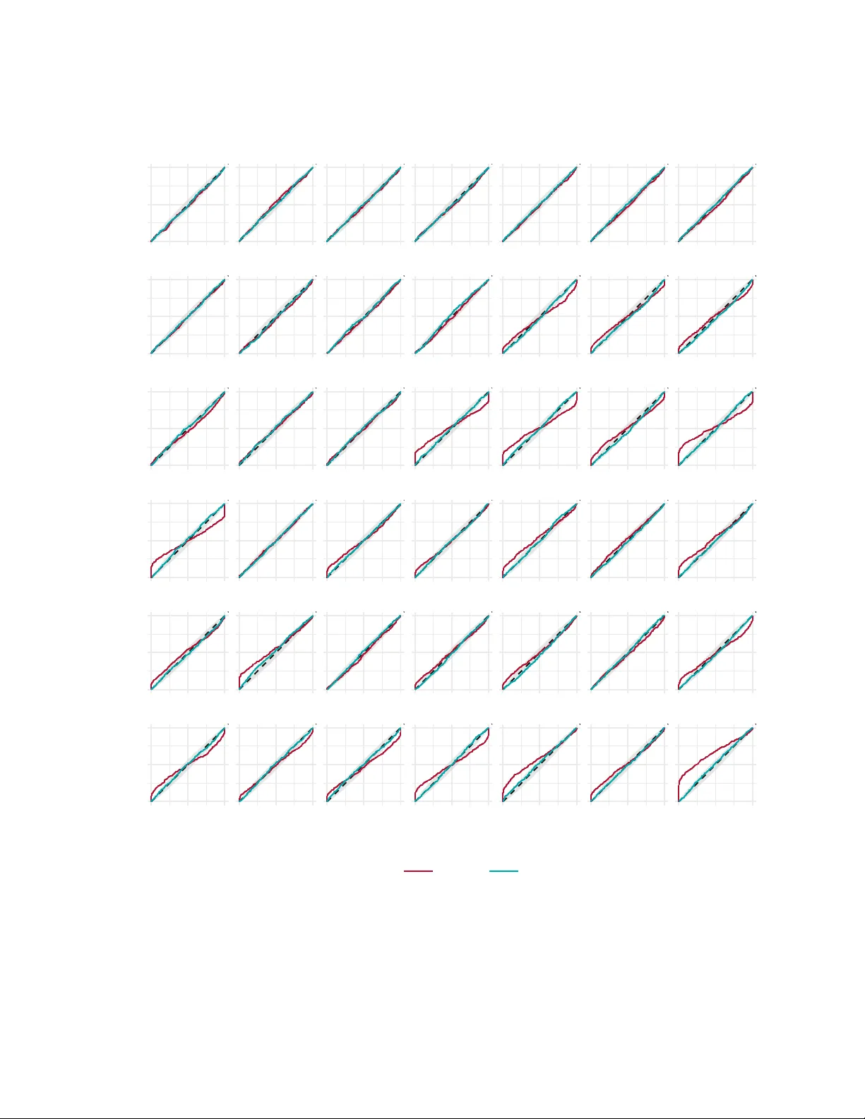
A P P R O X I M A T E B A Y E S I A N I N F E R E N C E F O R S T R U C T U R A L E Q UA T I O N M O D E L S U S I N G I N T E G R A T E D N E S T E D L A P L A C E A P P R O X I M A T I O N S A P R E P R I N T Haziq Jamil Computer , Electrical and Mathematical Sciences and Engineering (CEMSE) Division King Abdullah Univ ersity of Science and T echnology Thuwal, 23955-6900 Mathematical Sciences, Faculty of Science Univ ersiti Brunei Darussalam Bandar Seri Bega wan, BE 1410 haziq.jamil@kaust.edu.sa Håvard Rue Computer , Electrical and Mathematical Sciences and Engineering (CEMSE) Division King Abdullah Univ ersity of Science and T echnology Thuwal, 23955-6900 March 27, 2026 A B S T R AC T Markov chain Monte Carlo (MCMC) methods remain the mainstay of Bayesian estimation of structural equation models (SEM); ho wev er they often incur a high computational cost. W e present a bespoke ap- proximate Bayesian approach to SEM, drawing on ideas from the integrated nested Laplace approximation (INLA; Rue et al., 2009, J. R. Stat. Soc. Series B Stat. Methodol.) framework. W e implement a simpliﬁed Laplace approximation that ef ﬁciently proﬁles the posterior density in each parameter direction while correcting for asymmetry , allowing for parametric ske w-normal estimation of the marginals. Further- more, we apply a variational Bayes correction to shift the marginal locations, thereby better capturing the posterior mass. Essential quantities, including factor scores and model-ﬁt indices, are obtained via an adjusted Gaussian copula sampling scheme. For normal-theory SEM, this approach of fers a highly accurate alternativ e to sampling-based inference, achieving near -‘maximum likelihood’ speeds while retaining the precision of full Bayesian inference. K eywords Bayesian Structural Equation Model • Inte grated Nested Laplace Approximation (INLA) • Approximate Bayesian Inference • V ariational Bayes • Ske w-Normal Distribution A P R E P R I N T - M A R C H 2 7 , 2 0 2 6 1 Introduction Let y s ∈ R p denote the observed data vector for subject s = 1 , . . . , n , and deﬁne the stacked data vector y = ( y ⊤ 1 , . . . , y ⊤ n ) ⊤ . Although not the dominant presentation in continuous structural equation modelling (SEM) textbooks (Bollen, 1989 ; Hoyle, 2023 ; Kaplan, 2009 ; Skrondal & Rabe-Hesketh, 2004 ; Song & Lee, 2012 ), it is quite natural, particularly in the Bayesian paradigm, to e xpress SEMs as hierarchical latent Gaussian models (LGMs, Rue et al., 2009 ). Conditional on η = ( η ⊤ 1 , . . . , η ⊤ 1 ) ⊤ , each latent vector η s ∈ R q being associated with subject s , the data generating process is deﬁned by the following system of probabilistic models: y | η , ϑ 1 ∼ n Y s =1 ϕ ( y s ; ν + Λ η s , Θ ) (1) η | ϑ 2 ∼ n Y s =1 ϕ  ( I − B ) η s ; α , Ψ  (2) ϑ := { ϑ 1 , ϑ 2 } ∼ π ( ϑ ) (3) where ϕ ( · ; µ , Σ ) is the multiv ariate normal density with mean µ and cov ariance Σ , and π ( ϑ ) is a prior distribution ov er the model parameters ϑ ∈ R m . The SEM parameter vector ϑ collects the free entries of the v ectors and matrices governing the ﬁrst two le vels of the hierarchy in ( 1 ) and ( 2 ) . The ﬁrst lev el speciﬁes the measurement model , parameterised conditionally on the latent v ariables η by a p -vector of intercepts ν , a p × q factor loading matrix Λ (typically sparse), and a p × p error co variance matrix Θ . The second lev el deﬁnes the structural r elations among the latent variables, parameterised by the q × q matrix of regression coefﬁcients B , the q -vector of latent intercepts α , and the q × q cov ariance matrix of structural disturbances Ψ . W e assume measurement errors are independent of η s , and take B to be hollo w (i.e., diag( B ) = 0 q ). T ogether with the usual scale-setting constraints (e.g., ﬁxing one loading or factor v ariance per latent variable) and exclusion restrictions on Λ , B , and Ψ , these criteria yield a well-posed and (under standard regularity conditions) likelihood-identiﬁed parameterisation (Bollen & Davis, 2009 ). Moreov er , if B can be permuted to a strictly triangular form (equiv alently , the directed graph is acyclic), then ( I − B ) is in vertible, hence the structural system is algebraically well-deﬁned (Bentler & W eeks, 1980 ). In the Bayesian framew ork, inference on the SEM targets mainly the posterior distrib ution π ( ϑ | y ) ∝ Z π ( y | η , ϑ ) π ( η | ϑ ) π ( ϑ ) d η . (4) Direct ev aluation of this integral is generally intractable. T o circumvent high-dimensional inte gration, standard Markov Chain Monte Carlo (MCMC) algorithms e xploit the hierarchical structure of the LGM in ( 1 ) and ( 2 ) . by treating the latent variables η as missing data to be sampled. Conditioning on η simpliﬁes the likelihood, facilitating Gibbs or Metropolis-within-Gibbs sampling. Consequently , this approach has been widely adopted in software such as Mplus (Muthén & Asparouhov, 2012 ) and early blav aan implementations in R (Merkle & Rosseel, 2018 ) via J A GS (Plummer, 2003 ). Howe ver , the method necessitates augmenting the state space with the vector η , whose dimension scales linearly with the sample size n . This high dimensionality dri ves the substantial computational costs and poor mixing often observed in Bayesian SEM (Hecht et al., 2019 ; Lüdtke et al., 2018 ), regardless of whether the person-speciﬁc scores η are regarded as tar gets of inference or nuisance parameters (Hecht et al., 2020 ). Alternativ ely , the same hierarchical formulation in ( 1 ) and ( 2 ) . renders SEMs amenable to approximate Bayesian inference methods speciﬁcally designed for LGMs. The most prominent of these is the Integrated Nested Laplace Approximation (INLA, Rue et al., 2009 ). INLA capitalises on the conditional independence properties of the latent ﬁeld, formalising it as a Gaussian Marko v Random Field (GMRF , Rue & Held, 2005 ) often with sparse precision matrices, so 2 A P R E P R I N T - M A R C H 2 7 , 2 0 2 6 key computations reduce to sparse linear solv es and factorisations. The core strategy of INLA is to approximate ( 4 ) by ˜ π ( ϑ | y ) ∝ π ( y , η , ϑ ) ˜ π G ( η | y , ϑ )      η = η ∗ ( ϑ ) , (5) where ˜ π G ( η | y , ϑ ) is a Gaussian approximation of the full conditional π ( η | ϑ , y ) , and η ∗ ( ϑ ) is its mode. The marginal components of ( 5 ) are further approximated by ˜ π ( ϑ j | y ) = Z ˜ π ( ϑ | y ) d ϑ − j , j = 1 , . . . , m, (6) and the posterior marginals for the latent v ariables by ˜ π ( η s | y ) = Z ˜ π ( η s | y , ϑ ) ˜ π ( ϑ | y ) d ϑ , (7) in which ˜ π ( η s | ϑ , y ) is obtained through yet another Laplace-type approximation. The efﬁcienc y of INLA stems from a carefully constructed sequence of nested Laplace approximations and low-dimensional numerical integration schemes that turn these inte grals into accurate deterministic calculations. For comprehensi ve re vie ws of the methodology , we refer readers to Martins et al. ( 2013 ), Rue et al. ( 2017 ), and van Niek erk et al. ( 2023 ). Howe ver , for the linear Gaussian SEMs under consideration, we contend that retaining η as an explicit GMRF latent ﬁeld in the inference scheme is a suboptimal computational choice. While the GMRF representation is powerful in spatial or temporal settings where dependence is sparse and local (Krainski et al., 2018 ), standard SEMs typically induce a stacked latent ﬁeld with block-diagonal structure across subjects with dense within-block precision, limiting the gains from sparse-matrix algorithms. Moreover , correlated measurement errors (non-diagonal Θ ) break the conditional- independence structure that INLA exploits unless handled via latent augmentation (e.g., parameter expansion, Gelman, 2004 ; Palomo et al., 2007 ). W e propose that a f ar more efﬁcient strategy is to analytically inte grate out the latent v ariables entirely and target the marginal likelihood π ( y | ϑ ) directly . Due to the Gaussian conjugacy of the ﬁrst two lev els in ( 1 ) and ( 2 ) , this marginal likelihood is also Gaussian, i.e. π ( y | ϑ ) = Q n s =1 ϕ ( y s ; µ ( ϑ ) , Σ ( ϑ )) , where µ ( ϑ ) = ν + Λ ( I − B ) − 1 α (8) Σ ( ϑ ) = Λ ( I − B ) − 1 Ψ ( I − B ) −⊤ Λ ⊤ + Θ . (9) Furthermore, the conditional posterior π ( η | y , ϑ ) = Q n s =1 π ( η s | y s , ϑ ) appearing in ( 5 ), whose factors appear in ( 7 ), are all together e xact Gaussian densities as well. Each factor has a closed-form mean m s ( ϑ ) and cov ariance V ( ϑ ) giv en by m s ( ϑ ) = V  Φ − 1 ( I − B ) − 1 α + Λ ⊤ Θ − 1 ( y s − ν )  V ( ϑ ) =  Φ − 1 + Λ ⊤ Θ − 1 Λ  − 1 Φ := ( I − B ) − 1 Ψ ( I − B ) −⊤ . (10) This “collapsed” perspectiv e effecti vely reduces the inference problem to the lower-dimensional space of ϑ , bypassing the need to approximate a high-dimensional latent ﬁeld. The latent v ariables can easily be reco vered, either via empirical Bayes plugin estimates or post-hoc sampling. This realisation parallels the recent e volution of the blavaan R package. Merkle et al. ( 2021 ) noted that their initial data-augmentation implementation was often slo w for standard models. Shifting to a marginal likelihood approach for standard Gaussian SEMs using Stan (Stan Dev elopment T eam, 2026 ) yields improv ements in sampling efﬁcienc y and con ver gence stability , despite prev ailing literature advocating for the simplicity of sampling latent v ariables (e.g., Lee, 2007 ). 3 A P R E P R I N T - M A R C H 2 7 , 2 0 2 6 The primary contribution of this article is a framework for fast and accurate approximation of marginal posterior densities in normal-theory SEMs (Section 3 ), adapting k ey ideas from INLA to the SEM setting. The core is a simpliﬁed Laplace approximation that efﬁciently proﬁles the posterior along each parameter dimension. W e then reﬁne these proﬁles with parametric ske w-normal approximations to capture asymmetry , and apply a v ariational Bayes correction to improv e marginal location and posterior mass coverage. Finally , we use an efﬁcient Gaussian copula sampling scheme to propagate uncertainty to deri ved quantities of interest, including factor scores and model-ﬁt indices. The remainder of the paper is organised as follo ws. Section 2 re views the mathematical background, including the Laplace approximation and sk ew-normal distrib ution. Section 3 introduces the proposed methodology . Section 4 reports simulation results on parameter recovery , large-sample beha viour , and sensitivity to prior speciﬁcations. Section 5 discusses implications and future directions, and Section 6 concludes. 2 Preliminaries This section revie ws the technical tools on which the proposed methodology rests. 2.1 Laplace’ s Method Let x ∈ R d and y ∈ R n be vectors. In this subsection, vectors and matrices are shown in non-bold typeface for simplicity . Laplace’ s method (Ch 3.3, Barndorf f-Nielsen & Cox, 1989 ) provides accurate approximations to integrals of the form I = Z R d f ( y , x ) dx, f ( y , x ) > 0 by e xploting the fact that, when f ( y , · ) is suf ﬁciently concentrated, the integral is dominated by a neighbourhood around its maximiser . Assume that for each ﬁxed y , log f ( y , x ) has a unique mode x ∗ := x ∗ ( y ) and that the negati ve Hessian at the mode, H = −∇ 2 x log f ( y , x )    x = x ∗ , is positiv e deﬁnite ( H ≻ 0 ). A second-order T aylor expansion of log f ( y , x ) about x ∗ yields the Gaussian (quadratic) approximation, and integrating the resulting kernel with respect to x giv es I ≈ (2 π ) d/ 2 | H | − 1 / 2 f  y , x ∗  , or equiv alently , I ≈ f ( y , x = x ∗ ) ˜ π G ( x = x ∗   y ) , where ˜ π G ( x | y ) is the Gaussian density with mean x ∗ and precision H ( y ) . When the integrand admits the lar ge-sample representation I n = Z g ( y , x ) exp { nℓ ( y , x ) } dx, ℓ ( y , x ) = 1 n log f n ( y , x ) , with a unique interior maximiser and standard regularity conditions, Laplace’ s method yields an approximation ˜ I n that is asymptotically accurate with relativ e error O ( n − 1 ) , i.e. I n = ˜ I n { 1 + O ( n − 1 ) } (Rue et al., 2017 ), and hence log I n = log ˜ I n + O ( n − 1 ) . The accuracy of the Gaussian approximation is underpinned by the Bernstein-v on Mises theorem (see, e.g., van der V aart, 1998 ): for ﬁxed dimension, the posterior concentrates at rate n − 1 / 2 and con ver ges to a Gaussian in total v ariation, so a second-order expansi on of the log posterior around its mode becomes increasingly accurate. 2.2 Skew-Normal Distrib ution The ske w-normal (SN) distribution (Azzalini, 1985 ) extends the normal distrib ution by introducing a shape parameter that gov erns asymmetry , while retaining many of the tractable properties of the Gaussian family . 4 A P R E P R I N T - M A R C H 2 7 , 2 0 2 6 A random variable X follows a sk ew-normal distrib ution, written X ∼ SN ( ξ , ω , α ) , if its probability density function (PDF) is f SN ( x ; ξ , ω , α ) = 2 ω ϕ  x − ξ ω  Φ  α x − ξ ω  , x ∈ R , where ϕ ( · ) and Φ( · ) denote the standard normal density and distrib ution function, respectiv ely . The three parameters hav e the following roles: • ξ ∈ R is a location parameter; • ω > 0 is a scale parameter; and • α ∈ R is a shape (ske wness) parameter . When α = 0 the density reduces to N ( ξ , ω 2 ) ; positive (negati ve) v alues of α induce right (left) ske wness. The corresponding cumulativ e distribution function (CDF) does not admit a simple closed-form e xpression but can be written as F SN ( x ; ξ , ω , α ) = Φ  x − ξ ω  − 2 T  x − ξ ω , α  , where T ( h, a ) = (2 π ) − 1 R a 0 exp  − 1 2 h 2 (1 + t 2 )  / (1 + t 2 ) dt is Owen’ s T -function (Owen, 1956 ). Deﬁne δ = α/ √ 1 + α 2 . The mean, variance, and ske wness of X are E( X ) = ξ + ω δ r 2 π , V ar( X ) = ω 2  1 − 2 δ 2 π  , (11) Sk ew( X ) = 4 − π 2  δ p 2 /π  3  1 − 2 δ 2 /π  3 / 2 . (12) The coef ﬁcient of skewness is bounded in the interv al ( − 0 . 9953 , 0 . 9953) , which limits the degree of asymmetry that the SN family can represent. In practice, this range is more than adequate for the posterior mar ginals encountered in typical Bayesian applications. 3 Methodology W e no w describe a procedure for accurate, approximate Bayesian inference for normal-theory SEMs, consisting of four stages. First, we identify the posterior mode and construct an initial joint Laplace approximation. Second, we perform a deterministic marginalisation of the posterior that circumv ents high-dimensional numerical integration; this in volv es marginal proﬁling via axis scanning, v olume correction of the proﬁle densities, and ske w-normal curve ﬁtting. Third, we apply a V ariational Bayes (VB) correction to reﬁne the posterior location. Finally , we implement a Gaussian copula sampling scheme to estimate deriv ed quantities of interest. 3.1 Joint Laplace A pproximation In Bayesian analysis, Laplace’ s method is used to approximate intractable posterior normalising constants and posterior marginals (T ierney & Kadane, 1986 ). Write the posterior density for the SEM in ( 4 ) as π ( ϑ | y ) = π ( y | ϑ ) π ( ϑ ) π ( y ) , π ( y ) = Z π ( y , ϑ ) d ϑ , using the Gaussian likelihood for ϑ ∈ R m with mean and cov ariance as speciﬁed in ( 8 ) and ( 9 ) respectiv ely . W e then see that e valuating π ( y ) in volv es an integral of the Laplace form. An approximation to the posterior ˜ π G ( ϑ | y ) is thus locally Gaussian centred at the maximum a posteriori (MAP) estimate ϑ ∗ = arg max ϑ log π ( y , ϑ ) having precision H := H ( ϑ ∗ ) = −∇ 2 ϑ log π ( y , ϑ )    ϑ = ϑ ∗ ∈ R m × m , H ≻ 0 . (13) 5 A P R E P R I N T - M A R C H 2 7 , 2 0 2 6 The same quadratic expansion also deli vers a closed-form approximation to the associated normalising constant. In this case, it is the model evidence (mar ginal data density), which in log form is approximated by log π ( y ) ≈ m 2 log(2 π ) − 1 2 log | H | + log π ( y | ϑ ∗ ) + log π ( ϑ ∗ ) . (14) In implementation, parameters subject to positi vity or boundedness constraints (e.g., v ariances, correlations) are mapped to R via standard dif ferentiable transformations (log, Fisher), and all mode-ﬁnding, Hessian e valuation, and later on, marginal proﬁling, are carried out in this unconstrained parameter space. The corresponding Jacobian adjustments are applied at the ﬁnal step when reporting densities on their original scale. 3.2 Skew-Normal Laplace Pr oﬁling of Posterior Marginals If π ( ϑ | y ) were Gaussian, the joint Laplace approximation would be exact, and the univ ariate marginals would follo w immediately from standard properties of the multiv ariate normal distribution. In practice, SEM posteriors often exhibit ske wness and other departures from normality , particularly for variance and scale parameters (Muthén & Asparouho v, 2012 ). Curvature at the mode alone may fail to capture global asymmetry , with the discrepancy propagating to the marginal distrib utions. W e therefore e valuate the Laplace-proﬁled log marginal log ˜ π ( ϑ j | y ) on a grid for each j , and ﬁt a SN density to these ev aluations. For each component j = 1 , . . . , m , the marginal posterior is π ( ϑ j | y ) = Z π ( ϑ j , ϑ − j | y ) d ϑ − j , j = 1 , . . . , m, where ϑ − j denotes the vector of parameters ϑ with its j th element remov ed. Applying Laplace’ s method yet again to this integral gi ves the second-order approximation log ˜ π ( ϑ j | y ) = log π ( ϑ j , ϑ ∗ − j | y ) − 1 2 log | H − j ( ϑ j ) | + m − 1 2 log(2 π ) . The issue, ho wev er , is that direct ev aluation of this Laplace approximation is costly . For each grid point ϑ j one must (i) solv e an ( m − 1) -dimensional optimisation problem to obtain ϑ ∗ − j ( ϑ j ) , and (ii) compute log | H − j ( ϑ j ) | , where ϑ ∗ − j := ϑ ∗ − j ( ϑ j ) is the conditional maximiser and H − j ( ϑ j ) is the corresponding ( m − 1) × ( m − 1) negati ve Hessian matrix. The follo wing subsections describe a more ef ﬁcient strategy that a voids repeated optimisations and Hessian ev aluations while retaining salient marginal features, including ske wness. 3.2.1 Conditional Mean Path T o proﬁle the j th component ef ﬁciently , we replace repeated slice-wise optimisation by a deterministic trajectory through R m that tracks high posterior mass as ϑ j varies. This trajectory is the Conditional Mean P ath (CMP) , deﬁned as the locus of points where the remaining ( m − 1) nuisance parameters ϑ − j are set to their conditional expectations giv en ϑ j : C j =  ( x, ϑ − j ) ∈ R m   x ∈ R , ϑ − j = E ˜ π G [ ϑ − j | ϑ j = x ]  . Here, expectations are taken with respect to the Gaussian approximation ˜ π G ( ϑ | y ) from the joint Laplace step, and are av ailable in closed form. The rationale is that, for a multiv ariate normal target, marginalisation in ϑ − j is equiv alent (up to proportionality) to ev aluation along the CMP , as formalised in the following lemma (which also appears as Lemma 1 in Sec. 3.2.2 of Martins et al., 2013 ). Lemma 3.1 (Marginalisation via the CMP) . Let ϑ ∼ N m ( ϑ ∗ , Ω ) with Ω ≻ 0 . Then the mar ginal density of the j th component, j = 1 , . . . , m , is pr oportional to the joint density evaluated along its conditional mean path: π ( ϑ j = x ) ∝ π  ϑ j = x, ϑ − j = E[ ϑ − j | ϑ j = x ]  . 6 A P R E P R I N T - M A R C H 2 7 , 2 0 2 6 T o see this, note that the multi variate normal conditional e xpectation is afﬁne, E[ ϑ | ϑ j = x ] = ϑ ∗ + ( x − ϑ ∗ j ) Ω · j Ω j j , (15) where Ω · j is the j th column of Ω ; substituting into the joint quadratic form reduces it to ( x − ϑ ∗ j ) 2 / Ω j j , recov ering the marginal k ernel. The lemma provides an operational insight: for a Gaussian density , the exact marginal of ϑ j can be recov ered by slicing the joint density along the regression line of ϑ on ϑ j . For a non-Gaussian posterior , scanning along this linear trajectory serves as a ﬁrst-order approximation to a potentially curv ed ridge. W e therefore deﬁne our scan direction as follows. Let Ω denote the cov ariance matrix associated with the joint Laplace approximation, i.e. Ω = H − 1 with H as in ( 13 ). T o facilitate proﬁling, deﬁne the j th set of grid points G j =  ϑ ∗ + t v j   t ∈ [ − 4 , 4]  , v j = Ω · j p Ω j j . (16) Here, the direction vector v j is normalised so that t acts as a Z -score for ϑ j : a unit step t = 1 induces a displacement of one standard de viation p Ω j j in the j th coordinate, while the remaining ( m − 1) components adjust according to their linear dependence on ϑ j via Ω · j . T aking t ∈ [ − 4 , 4] thus spans ± 4 standard deviations in this scan direction, cov ering about 99.994% of the corresponding Gaussian mass. 3.2.2 Efﬁcient V olume Correction Evaluating log π ( ϑ | y ) along G j replaces the Gaussian quadratic decay implied by the joint Laplace approximation with the actual slice-wise peak log-density (“height”) as ϑ j v aries. Accurate marginalisation, ho we ver , also requires the Laplace volume correction − 1 2 log | H − j ( ϑ j ) | , which captures changes in the conditional spread of ϑ − j orthogonal to the scan direction. W e now show how to update this volume term ef ﬁciently along the grid without full Hessian re-ev aluations. Consider again the scan trajectory ϑ ( t ) = ϑ ∗ + t v j used to proﬁle the j th posterior marginal on the grid G j . Write H − j ( t ) for the ( m − 1) × ( m − 1) submatrix of H ( t ) := H ( ϑ ( t )) with the j th row and column remo ved, and deﬁne γ j ( t ) := − 1 2 log   H − j ( t )   . A ﬁrst-order expansion yields γ j ( t ) ≈ γ j (0) + t γ ′ j (0) , so that along G j the volume term can be updated from the slope γ ′ j (0) . Since γ j (0) is constant in t , it contributes only an additiv e shift to the log-mar ginal along G j . This offset is handled automatically by the intercept (normalising) term in the subsequent ske w-normal ﬁt. As a remark, higher-order expansions of γ j ( t ) are possible, but we focus on the ﬁrst-order update here; implications are discussed in Section 5 . The following lemma shows that the slope γ ′ j (0) admits the form of a projected trace of the whitened Hessian perturbation at the mode. Lemma 3.2 (V olume-slope decomposition) . Let z = L − 1 ( ϑ − ϑ ∗ ) with H ( ϑ ∗ ) − 1 = LL ⊤ , and write J ( t ) = L ⊤ H ( t ) L for the ne gative Hessian in whitened coordinates along the scan trajectory . Let w j = L − 1 v j denote the image of the scan dir ection in the whitened frame . Then J := J (0) = I m , ∥ w j ∥ = 1 , and γ ′ j (0) = − 1 2 tr( J ′ ) + 1 2 w ⊤ j J ′ w j , (17) wher e J ′ := J ′ (0) = d dt J ( t )   t =0 . Equiv alently , writing P ⊥ j = I m − w j w ⊤ j for the projector onto the orthogonal complement of w j , γ ′ j (0) = − 1 2 tr  P ⊥ j J ′  . The geometric content is apparent: the v olume slope measures the rate of curvature change in the whitened frame, restricted to directions transverse to the scan. Since J = I m , the whitening renders all baseline curvatures unity , so the formula reduces entirely to traces of the ﬁrst-order perturbation J ′ . And, this result is independent of the choice of the 7 A P R E P R I N T - M A R C H 2 7 , 2 0 2 6 whitening matrix L . The next corollary shows ho w these quantities can be ev aluated efﬁciently using only gradient information. Corollary 3.1 (Gradient representation of the v olume slope) . Let g ( ϑ ) = −∇ ϑ log π ( ϑ | y ) , so that H ( ϑ ) = ∇ ϑ g ( ϑ ) and u ⊤ H ( ϑ ) u = u ⊤ d d u g ( ϑ ) for any ﬁxed dir ection u . Then the volume slope ( 17 ) admits the gradient r epr esentation γ ′ j (0) = − 1 2 m X k =1 d dt  L ⊤ · k d d L · k g  t =0 + 1 2 d dt  v ⊤ j d d v j g  t =0 , (18) wher e L · k is the k th column of L . The m summands r esolve the tr ace in ( 17 ) column by column, and the ﬁnal term is its Schur corr ection. Ev aluating each part in ( 18 ) in volves two ﬁnite-dif ference layers, both anchored at the mode where H ( ϑ ∗ ) = ( L ⊤ L ) − 1 : an inner perturbation by step size δ along each of the m + 1 directions u ∈ { L · 1 , . . . , L · m , v j } , approximating the bracketed terms d d u g ; and an outer perturbation by step size ε along the scan direction v j , approximating the deriv ativ e in t . Both reduce to ev aluations of g ( ϑ ) alone, without e ver forming or factoring H ( ϑ ) . Since the whitening renders all m + 1 baseline curv atures unity at the mode, a forward-dif ference scheme is particularly economical. The outer layer needs only a single shifted point ϑ + = ϑ ∗ + ε v j , differenced against the known baseline of 1 at the mode. At ϑ + , a single base gradient g ( ϑ + ) is shared across all m + 1 inner perturbations, each dif ferenced against one additional ev aluation g ( ϑ + + δ u ) . The total cost is therefore just m + 2 gradient e valuations per scan direction j . Both layers can be independently upgraded to central dif ferences for improved accuracy; upgrading the inner layer alone costs 2( m + 1) e valuations, as the shared base at ϑ + is replaced by a symmetric pair around each direction. 3.2.3 Skew-Normal Curv e Fitting The grid e valuations from the pre vious sections provide a discrete approximation to each mar ginal log-posterior . W e con vert these ordinates into a smooth, normalised approximation by ﬁtting a ske w-normal density , which provides a parametric unimodal family capable of capturing moderate ske wness. Fix j ∈ { 1 , . . . , m } . Let G j = { ϑ ( t k ) } K k =1 be the K points on the scan grid from ( 16 ), ordered along the scan direction v j , with t k ∈ [ − 4 , 4] . Combining the height ev aluation with the linearised volume correction yields the unnormalised, volume-corrected log-mar ginal ordinates h kj := log π  ϑ ( t k ) | y  + t k γ ′ j (0) , ϑ ( t k ) ∈ G j , where γ ′ j (0) is the slope of the v olume term deriv ed in the previous subsection. From the pairs { ( ϑ j ( t k ) , h kj ) } K k =1 , we approximate the marginal density of ϑ j by a skew-normal distribution SN ( ξ j , ω j , α j ) . Since the values h kj are log-density ordinates deﬁned only up to an additiv e constant, we include a free intercept c j and ﬁt by weighted least squares: ( ˆ ξ j , ˆ ω j , ˆ α j , ˆ c j ) = arg min ξ,ω ,α,c K X k =1 ω kj  h kj −  log f SN ( ϑ j ( t k ); ξ , ω , α ) + c j  2 . A con venient default is to weight points by their implied mass, ω kj ∝ exp( h kj ) , which prioritises ﬁdelity near the mode; alternative weightings may be used to emphasise tail behaviour . W ith the normalised approximation ˜ π ( ϑ j | y ) ∝ f SN ( ϑ j ; ˆ ξ j , ˆ ω j , ˆ α j ) , posterior summaries (means, standard de viations, and quantiles) are computed using standard formulae or by direct numerical in version of the ﬁtted CDF . 3.3 V ariational Mean Correction of the Laplace Appr oximation The joint Laplace approximation ϑ | y ≈ N m ( ϑ ∗ , Ω ) , with Ω = H ( ϑ ∗ ) − 1 , can misrepresent the typical set when the posterior mode is not a representativ e centre of mass, leading to point summaries that sit a way from the bulk of posterior probability . V ariational Bayes (VB) offers a principled remedy by recasting inference as an optimisation 8 A P R E P R I N T - M A R C H 2 7 , 2 0 2 6 problem (Knoblauch et al., 2022 ): among all densities in a tractable family , ﬁnd the one that is “closest” to the true posterior , as measured by the Kullback-Leibler di ver gence (KLD). As a simple, low-cost reﬁnement, we adopt the VB mean-shift correction of van Niek erk and Rue ( 2024 ), which keeps Ω ﬁxed and estimates a location shift δ ∈ R m by ˆ δ = arg min δ D KL  N m ( ϑ ∗ + δ , Ω ) ∥ π ( · | y )  . (19) The choice of KLD as the discrepancy measure is not arbitrary . Zellner ( 1988 ) showed that minimising D KL ( q ∥ π ) is the unique “optimal information-processing rule” that minimises information loss when summarising a distribution π by a tractable proxy q . Rather than constructing a v ariational approximation q from scratch, we reﬁne the e xisting Gaussian approximation by holding its cov ariance ﬁxed at its Laplace v alue Ω . Under this constraint, the only free degree of freedom is a location shift, which a voids the substantial cost of re-estimating an m × m cov ariance matrix. Minimising the KLD ( 19 ) over δ is equiv alent to maximising an expected log-posterior under the shifted Gaussian. Indeed, D KL ( q δ ∥ π ( · | y )) = E q δ  log q δ ( ϑ )  − E q δ  log π ( ϑ | y )  , and since q δ ( ϑ ) = ϕ m ( ϑ ; ϑ ∗ + δ , Ω ) has cov ariance Ω ﬁxed, its entropy (hence E q δ [log q δ ] ) is constant in δ . Therefore ˆ δ can be obtained by maximising the e xpected log posterior , ˆ δ = arg max δ ∈ R m E ϑ ∼N m ( ϑ ∗ + δ , Ω )  log π ( ϑ | y )  . (20) The expectation in ( 20 ) decomposes as E q δ [log π ( y | ϑ )] + E q δ [log π ( ϑ )] . Any component that is quadratic in ϑ contributes a closed-form term by conjugac y; the remaining non-quadratic components—mainly the non-Gaussian priors (e.g., the Gamma and Beta families in T able 1 ) and a nonlinear lik elihood—require numerical treatment. This can be approximated reliably using a randomised quasi-Monte Carlo (RQMC) rule (L ’Ecuyer, 2018 ), e.g. via scrambled Sobol points mapped elementwise to N(0 , 1) by a probit transform, yielding a lo w-discrepancy sample-average objectiv e. As in Lemma 3.2 , we may carry out the maximisation ( 20 ) in a whitened parameterisation, which typically impro ves numerical conditioning. Finally , the VB correction is applied as a post-processing translation of location summaries. The proﬁling and volume- correction steps remain anchored at the mode ϑ ∗ , as required by the local expansions; the correction merely shifts the resulting marginal approximations by ˆ δ while preserving their ﬁtted shape parameters. 3.4 Gaussian Copula Sampling The preceding steps deliv er closed-form approximations for the marginal posteriors π ( ϑ j | y ) , j = 1 , . . . , m , via ﬁtted ske w-normal distributions. For inference that depends only on a single-component monotonic transformation of them (e.g., ϑ j 7→ exp( ϑ j ) for variances), these mar ginals sufﬁce. Quantiles follo w by transformation of the ﬁtted CDF , and one-dimensional expectations can be e valuated directly (e.g., by quadrature). For inference inv olving transformations of multiple parameters simultaneously , we require an approximation to the joint dependence structure. One could sample directly from the joint Laplace Gaussian N m ( ϑ ∗ , Ω ) , but this w ould discard the marginal accuracy gained in the preceding steps, rev erting each component to a Gaussian marginal. Since our methodology targets marginal accuracy while retaining only a local Gaussian approximation of dependence at the mode, we instead reconstruct joint posterior samples using a Gaussian copula (Nelsen, 2006 ) with the ﬁtted ske w-normal marginals. Let Ω = H ( ϑ ∗ ) − 1 denote the co variance matrix from the joint Laplace approximation, and deﬁne the associated correlation matrix R = D − 1 / 2 Ω D − 1 / 2 , D = diag ( Ω ) . 9 A P R E P R I N T - M A R C H 2 7 , 2 0 2 6 Let F ( j ) SN denote the ﬁtted ske w-normal CDF for the j th marginal, and Q ( j ) SN ( τ ) = inf { x | F ( j ) SN ( x ) ≥ τ } the correspond- ing quantile function. For b = 1 , . . . , B , a joint draw ϑ ( b ) is obtained by: 1. Copula draw: Sample z ( b ) ∼ N m ( 0 , R ) ; 2. Probability integral transf orm: Set u ( b ) j = Φ( z ( b ) j ) , j = 1 , . . . , m ; 3. Marginal in version: Set ϑ ( b ) j = Q ( j ) SN ( u ( b ) j ) , j = 1 , . . . , m . This construction preserv es the ﬁtted skew-normal marginal shapes by design. Ho wev er , when the marginals are sk ewed (i.e. α j  = 0 ), the nonlinear quantile transforms in Step 3 distort the Pearson correlations of the output away from the Laplace target R . T o correct for this, we apply the NOR T A (NORmal T o Anything) adjustment of Cario and Nelson ( 1997 ). For each ( j, k ) pair , we solve for a latent correlation R ∗ j k such that the induced correlation between the transformed variables matches the tar get R j k : Cor  Q ( j ) SN (Φ( z j )) , Q ( k ) SN (Φ( z k ))  = R j k , z j z k ! ∼ N 2 0 , 1 R ∗ j k R ∗ j k 1 !! . The induced correlations are e valuated via tw o-dimensional Gauss-Hermite quadrature, and the  m 2  uni-dimensional root problems are solved independently . The adjusted matrix R ∗ then replaces R in Step 1, ensuring that the joint samples hav e both the correct skew-normal marginals and Pearson correlations matching the Laplace cov ariance structure. The resulting samples can be used to approximate posterior expectations of multiv ariate functionals g ( ϑ ) (e.g., nonlinear parameter constraints, deriv ed quantities such as indirect ef fects, or other model-based transformations) and to propagate uncertainty through do wnstream SEM computations in the usual Bayesian manner . If desired, one may retain a parametric representation for an y deri ved scalar quantity g ( ϑ ) by ﬁtting a ske w-normal approximation to its copula-based samples (e.g., by moment matching or maximum likelihood), yielding a smooth, parsimonious summary in place of histogram-based estimates. 4 V alidation Study This section details the v alidation study , organised into subsections describing the design and benchmark model and prior speciﬁcation, computational note, MCMC comparison, and the simulation study results. 4.1 Benchmark Model and Priors W e use the Political Democracy model of Bollen ( 1989 ) as a benchmark, owing to its long-standing role as a canonical structural equation model with both measurement and structural components and a modest sample size ( n = 75 ). The model comprises two latent constructs measured by multiple observ ed indicators, coupled with a structural regression linking the latent v ariables (see Figure 1 ). Its ubiquity in the SEM literature and the availability of widely reported estimates make it a conv enient reference point for assessing approximate Bayesian inference. In total, m = 42 parameters are estimated in this SEM, including the means of the observations. Priors are speciﬁed to be weakly regularising, ensuring posterior propriety and numerical stability without being tuned to the proposed approximation. W e adapt the default prior families commonly used in Bayesian SEM software (as implemented in blav aan), assigning diffuse Gaussian priors to unconstrained coefﬁcients (e.g., loadings and regression effects) and weakly informativ e priors to (co)variance components, with cov ariance structures parameterised via standard de viations and correlations. All priors are speciﬁed independently across estimable parameters, and they are ﬁxed a priori and held constant across the benchmark and subsequent simulation studies. T able 1 lists the diffuse priors used for the benchmark and simulation studies, alongside an informati ve prior speciﬁcation used in the calibration analysis of Section 4.5 . 10 A P R E P R I N T - M A R C H 2 7 , 2 0 2 6 η 1 η 2 η 3 y 1 y 2 y 3 y 4 y 5 y 6 y 7 y 8 y 9 y 10 y 11 1 1 1 1 1 1 1 1 1 1 1 ν 1 ν 2 ν 3 ν 4 ν 5 ν 6 ν 7 ν 8 ν 9 ν 10 ν 11 Λ 1 , 1 Λ 2 , 1 Λ 3 , 1 Λ 4 , 1 Λ 5 , 2 Λ 6 , 2 Λ 7 , 2 Λ 8 , 2 Λ 9 , 3 Λ 10 , 3 Λ 11 , 3 B 3 , 1 B 1 , 2 B 3 , 2 Θ 1 , 5 Θ 2 , 6 Θ 3 , 7 Θ 4 , 8 Θ 2 , 4 Θ 6 , 8 Θ 1 , 1 Θ 2 , 2 Θ 3 , 3 Θ 4 , 4 Θ 5 , 5 Θ 6 , 6 Θ 7 , 7 Θ 8 , 8 Θ 9 , 9 Θ 10 , 10 Θ 11 , 11 Ψ 1 , 1 Ψ 2 , 2 Ψ 3 , 3 Figure 1: Path diagram for the Political Democracy SEM (Bollen, 1989 ). Circles denote latent v ariables; squares denote observed indicators. Single-headed arrows represent factor loadings ( Λ i,j ) and structural regression coef ﬁcients ( B j,j ′ ). Double-headed arrows represent residual v ariances ( Θ i,i ), residual covariances ( Θ i,j , i  = j ), and latent v ariances ( Ψ j,j ). The diagram depicts the model for a single observation; the same structure is assumed independently for each s = 1 , . . . , n . T able 1: Prior speciﬁcation for the benchmark SEM model. The diffuse priors are used throughout the benchmark and simulation studies; the informativ e priors are used in the SBC analysis (Section 4.5 ). Parameter T ype Diffuse Informativ e ν i Observed intercept N(0 , 32 2 ) N(0 , 32 2 ) α j Latent intercept N(0 , 10 2 ) N(0 , 10 2 ) Λ i,j Loading N(0 , 10 2 ) N(1 . 25 , 0 . 25 2 ) B j,j ′ Regression coef ﬁcient N(0 , 10 2 ) N(1 . 5 , 0 . 25 2 ) Θ 1 / 2 i,i Residual standard deviation Γ(1 . 0 , 0 . 5) Γ(10 , 10) Ψ 1 / 2 j,j Latent standard deviation Γ(1 . 0 , 0 . 5) Γ(10 , 10) ρ i,j Correlations associated with cov ariances Beta (1 , 1) Beta (5 , 5) 11 A P R E P R I N T - M A R C H 2 7 , 2 0 2 6 4.2 Computational Note All analyses were conducted in R version 4.5.2 (R Core T eam, 2025 ). The proposed INLA-based approximation is implemented in the R package INLA vaan (Jamil, 2026 ). For MCMC, we depended on the R package blav aan (Merkle et al., 2021 ), which uses Stan’ s Hamiltonian Monte Carlo sampler (Stan De velopment T eam, 2026 ). Computations were performed on a MacBook Pro (Apple M4 Pro, 14-core CPU, 24 GB uniﬁed RAM). 4.3 Comparison to MCMC W e assess the accuracy of the proposed deterministic approximation on the canonical benchmark model by comparison to a high-accuracy MCMC baseline. The ev aluation tar gets the full set of mar ginal posteriors { π ( ϑ j | y ) } m j =1 , with particular emphasis on uncertainty summaries and on the ﬁdelity of the marginal density shape. MCMC samples were obtained with 3 independent chains, 5,000 warmup iterations per chain and 10,000 post-warmup draws per chain. Con ver gence diagnostics indicated excellent mixing: b R = 1 . 00 for all parameters and a minimum total effecti ve sample size of 9,646. Each MCMC chain took roughly 27.9 seconds to con verge. Our proposed INLA-based approximation completed inference in 1.68 seconds in total. Breaking this down further , the joint Laplace approximation (mode-ﬁnding and Hessian forming) took 99 ms; VB correction step took 103 ms; the marginal construction took 1.1 s for the 42 parameters in serial; the NOR T A adjustments took 172 ms for 861 pairs of correlations; and the copula sampling (for six cov ariance parameters) took 142 ms. For each parameter ϑ j , we compute absolute errors between the approximation and MCMC for the posterior mean, standard de viation, median, central 95% interv al endpoints ( q 0 . 025 , q 0 . 975 ) , and mode. Errors are aggregated by parameter class and summarised by medians and maxima across parameters within each class (T able 2 ). In addition, we report a standardised mean discrepancy , | ∆ Mean | SD MCMC = | E approx ( ϑ j ) − E MCMC ( ϑ j ) | SD MCMC ( ϑ j ) , which expresses mean error relati ve to posterior uncertainty . V alues well belo w 1 indicate approximation error that is small compared to posterior dispersion. T o assess the agreement of full mar ginal shapes, we compute a symmetric div ergence between the mar ginal densities implied by the approximation and MCMC. Let p j denote the approximating marginal density (from the ﬁtted ske w- normal) and let q j denote a smooth density estimate from MCMC draws. W e report the Jensen–Shannon (JS) diver gence JSD( p j , q j ) = 1 2 D KL ( p j ∥ m j ) + 1 2 D KL ( q j ∥ m j ) , m j = 1 2 ( p j + q j ) , and present results as a bounded “percent discrepancy” 100 ×  1 − JSD( p j ,q j ) log 2  ∈ [0 , 100] , where 100% indicates identical distributions. Figure 2 visualises representativ e marginals across parameter blocks, overlaying the ﬁtted ske w-normal approximation with the MCMC density . Overall, the proposed approximation sho ws strong agreement with the MCMC reference across all parameter classes (T able 2 ). Median standardised discrepancies | ∆ Mean | / SD MCMC are all below 0.06 across all parameter classes, and the single largest v alue observed across all 42 parameters is 0.22 posterior standard deviations—well within the range that would lea ve substanti ve inference unaf fected. Intercepts, loadings, and regression coef ﬁcients are recov ered with negligible error: mean absolute errors for posterior means and central quantiles are at or belo w the third decimal place, as expected gi ven that these location-scale parameters typically yield approximately symmetric, well-behaved posteriors. Some what larger discrepancies arise for v ariance and cov ariance parameters, particularly in the tail quantiles ( q . 025 , q . 975 ), reﬂecting the limited ﬂexibility of the ske w-normal family in capturing the shape of distributions that are bounded belo w at zero and often exhibit pronounced right ske w . Importantly , even for these components the errors remain small in absolute terms, especially for posterior means and medians, which are the summaries most commonly used in applied SEM inference. 12 A P R E P R I N T - M A R C H 2 7 , 2 0 2 6 T able 2: Mean absolute error (MAE) is reported for each posterior summary quantity (mean, standard deviation, quantiles, and mode) aggregated by parameter class. The standardised discrepancy | ∆ Mean | / SD MCMC expresses the absolute error of the posterior mean in units of the MCMC posterior standard deviation; values belo w 0.25 indicate negligible approximation error relati ve to posterior uncertainty . N denotes the number of parameters in each class. MAE (absolute) | ∆ Mean | / SD MCMC Parameter N Mean SD q . 025 q . 50 q . 975 Mode Max | ∆ Mean | Median Max Observed intercepts 11 0.001 0.010 0.025 0.002 0.017 0.021 0.003 0.002 0.007 Loadings 8 0.010 0.016 0.013 0.007 0.051 0.009 0.014 0.049 0.078 Regressions 3 0.006 0.009 0.017 0.005 0.019 0.019 0.007 0.019 0.048 Residual variances 11 0.018 0.022 0.042 0.016 0.062 0.047 0.037 0.037 0.218 Residual cov ariances 6 0.019 0.028 0.047 0.029 0.094 0.071 0.027 0.029 0.062 Latent variances 3 0.031 0.031 0.072 0.034 0.039 0.055 0.053 0.053 0.183 ∆ = INLA − MCMC. MCMC: 3 chains, 10 000 post-warmup draws each. The density ov erlays in Figure 2 corroborate these ﬁndings. JS similarity exceeds 99% for the majority of parameters, and the minimum across all 42 marginals is 98.5% ( Θ 10 , 10 ), conﬁrming close distributional agreement throughout. Inspection of the cases with the lowest similarity re veals their sources. V ariance marginals (e.g. Θ 10 , 10 and Ψ 2 , 2 ) exhibit an upw ard inﬂection of the MCMC density near zero, consistent with the sampler encountering the positi vity boundary—a hallmark of near-Heyw ood conditions. A unimodal skew-normal density cannot reproduce this boundary pile-up, yet it compensates by concentrating mass in the re gion of highest posterior probability , preserving the ﬁdelity of central summaries. The latent variance Ψ 2 , 2 displays a notably elongated right tail in the MCMC reference, suggestiv e of weak identiﬁcation of that variance component or insuf ﬁcient prior regularisation in that direction; the skew-normal approximation captures the bulk of this distrib ution but necessarily under -represents the extreme tail. It is worth noting that the Political Democracy model, with its modest sample size ( n = 75 ), non-tri vial structural component, and six residual cov ariances, constitutes a challenging benchmark for any approximate method. The consistently high ﬁdelity observed here therefore provides an encouraging indication of real-world performance for the class of SEMs most commonly encountered in practice. 4.4 Simulation Study W e complement the single-dataset comparison with a repeated-sampling study that e v aluates calibration and sharpness of the approximate posteriors when the true parameter v ector is kno wn. Data were generated from the Political Democracy model speciﬁcation in Figure 1 using a kno wn true parameter vector ϑ 0 set to a bias-reduced regularised maximum likelihood estimate (Jamil et al., 2026 ). This choice mitigates the well-kno wn small-sample bias of the MLE, particularly for variance and cov ariance parameters, ensuring that the data-generating mechanism does not artiﬁcially fav our or penalise any particular inference method. Six sample sizes were considered: n ∈ { 75 , 150 , 300 , 600 , 1200 , 2400 } , with B = 250 independent replications at each n . The proposed approximation was applied to e very generated dataset using the same model and prior speciﬁcation as in the benchmark analysis. The entire simulation study completed in approximately four and a half minutes. T o k eep the presentation focused, we report results for ﬁ ve representati ve parameters, one from each estimable class (excluding observ ed intercepts, which are rarely of substantive interest): a factor loading ( Λ 3 , 1 ), a structural regression coefﬁcient ( B 2 , 3 ), a residual variance ( Θ 10 , 10 ), a residual cov ariance ( Θ 1 , 5 ), and a latent disturbance variance ( Ψ 2 , 2 ). For each replication and parameter, we record (i) the 95% and 50% credible interv al coverage rates (CR95 and CR50), deﬁned as the proportion of replications in which the respecti ve credible interval contains ϑ 0 ,j ; and (ii) the mean log score (MLS), B − 1 P B b =1 log ˜ π ( b ) ( ϑ 0 ,j | y ( b ) ) , which jointly penalises miscalibration and lack of sharpness. 13 A P R E P R I N T - M A R C H 2 7 , 2 0 2 6 100% 99.9% 99.1% 99.6% 100% 99.7% 99.5% 99.9% 99.9% 99.1% 98.8% 99.7% 98.5% 99.5% 99.9% 99.9% 99.5% 99.9% 99.9% 99.9% 99.8% 99.9% 99.9% 99.3% 99.8% 100% 99.6% 99.6% 100% 99.9% 99.1% 99.8% 99.9% 99.6% 98.9% 99.9% 99.0% 99.5% 99.9% 99.8% 99.5% 99.8% Θ 3,7 Θ 4,8 Θ 6,8 Ψ 1,1 Ψ 2,2 Ψ 3,3 Θ 9,9 Θ 10,10 Θ 11,11 Θ 1,5 Θ 2,4 Θ 2,6 Θ 3,3 Θ 4,4 Θ 5,5 Θ 6,6 Θ 7,7 Θ 8,8 Λ 11,3 B 2,1 B 1,3 B 2,3 Θ 1,1 Θ 2,2 Λ 3,1 Λ 4,1 Λ 6,2 Λ 7,2 Λ 8,2 Λ 10,3 ν 7 ν 8 ν 9 ν 10 ν 11 Λ 2,1 ν 1 ν 2 ν 3 ν 4 ν 5 ν 6 −2 0 2 4 −2 0 2 4 −1 0 1 2 3 4 2.5 5.0 7.5 10.0 0 1 2 3 4 5 0.2 0.4 0.6 0.8 1.0 0.05 0.10 0.15 0.20 0.00 0.25 0.50 0.75 0.3 0.6 0.9 −1 0 1 2 3 0 2 4 6 0 2 4 6 2.5 5.0 7.5 10.0 0.0 2.5 5.0 7.5 2 4 6 4 6 8 10 2 4 6 8 2 4 6 8 1.5 2.0 2.5 0.6 0.9 1.2 1.5 0 1 2 3 −0.5 0.0 0.5 1.0 1.5 2 4 6 5 10 15 0.5 1.0 1.5 2.0 1.0 1.5 2.0 2.5 3.0 0.5 1.0 1.5 2.0 2.5 1.0 1.5 2.0 2.5 1.0 1.5 2.0 2.5 1.6 2.0 2.4 2.8 5 6 7 8 3 4 5 4.75 5.00 5.25 4.0 4.5 5.0 5.5 2.8 3.2 3.6 4.0 1 2 3 4 5 6 3 4 5 6 5 6 7 8 3 4 5 6 4.0 4.5 5.0 5.5 6.0 6.5 2 3 4 0.00 0.25 0.50 0.75 1.00 0.0 0.5 1.0 1.5 2.0 0 1 2 0.0 0.1 0.2 0.3 0.0 0.2 0.4 0.0 0.2 0.4 0 1 2 3 4 0.0 0.5 1.0 0.0 0.5 1.0 1.5 2.0 2.5 0.0 0.5 1.0 1.5 2.0 0.0 0.2 0.4 0.6 0.8 0.0 0.2 0.4 0.0 0.2 0.4 0.6 0 1 2 3 0.00 0.25 0.50 0.75 1.00 0.0 0.5 1.0 1.5 2.0 0.0 0.5 1.0 1.5 2.0 2.5 0.0 0.5 1.0 1.5 0.0 0.1 0.2 0.3 0.4 0.00 0.25 0.50 0.75 1.00 0.0 0.1 0.2 0.3 0.4 0.0 0.3 0.6 0.9 0 1 2 3 4 0.0 0.5 1.0 1.5 2.0 0.00 0.25 0.50 0.75 1.00 0.0 0.2 0.4 0.6 0.8 0 1 2 3 4 0.0 0.2 0.4 0.6 0.00 0.25 0.50 0.75 0.0 0.3 0.6 0.9 0.0 0.5 1.0 1.5 2.0 2.5 0 1 2 3 4 0.0 0.1 0.2 0.3 0.4 0.5 0 2 4 6 0.00 0.25 0.50 0.75 0.0 0.5 1.0 0.00 0.25 0.50 0.75 1.00 0 1 2 0 1 2 0.0 0.1 0.2 0.3 0.4 0 5 10 15 20 0.0 0.2 0.4 0.6 INLA MCMC Figure 2: Marginal posterior densities for the Political Democracy SEM. Solid curves show the ﬁtted sk ew-normal approximation; shaded densities are kernel density estimates from MCMC. Percentages indicate JS similarity , with values near 100% reﬂecting close distrib utional agreement. W ell-calibrated posteriors should yield CR95 ≈ 95% and CR50 ≈ 50%, while improving log scores reﬂect increasing posterior concentration around the truth as n gro ws. Results are shown in Figure 3 . Cov erage at the 95% level is close to nominal throughout: CR95 ranges from 90% to 96% across all 30 parameter– sample-size cells, with the majority close to 95%. No systematic over - or under-cov erage is apparent, conﬁrming that the approximate 95% credible interv als are well calibrated under repeated sampling. Coverage at the 50% le vel is like wise stable, hov ering between 44% and 54% with a central tendency near the nominal 50%, though modest departures are visible for certain variance parameters (e.g., Θ 10 , 10 and Ψ 2 , 2 ). These small de viations are consistent with the limited ability of the sk ew-normal f amily to capture the asymmetric shape of near -boundary variance posteriors, which affects the precise placement of central quantiles more than it does the outer tails. Mean log scores increase monotonically with sample size for every parameter , rising from values near or below zero at n = 75 to values e xceeding 1.2–2.9 at n = 2400 . This conﬁrms that the approximate posteriors sharpen appropriately as data accumulate, and that lar ger samples yield more concentrated mar ginals that assign greater density to the true value. The rate of improv ement varies by parameter class. Location parameters ( Λ 3 , 1 , B 2 , 3 ) exhibit steady gains, while 14 A P R E P R I N T - M A R C H 2 7 , 2 0 2 6 MLS = 0.38 CR95 = 92% CR50 = 52% MLS = 0.75 CR95 = 93% CR50 = 46% MLS = 1.15 CR95 = 96% CR50 = 47% MLS = 1.48 CR95 = 96% CR50 = 47% MLS = 1.82 CR95 = 96% CR50 = 45% MLS = 2.21 CR95 = 95% CR50 = 46% Λ 3,1 1 2 3 0 1 2 3 4 0 1 2 3 4 5 0 2 4 6 0.0 2.5 5.0 7.5 0.0 2.5 5.0 7.5 10.0 12.5 0 5 10 15 P oster ior density MLS = 0.06 CR95 = 96% CR50 = 48% MLS = 0.39 CR95 = 93% CR50 = 50% MLS = 0.77 CR95 = 95% CR50 = 50% MLS = 1.11 CR95 = 95% CR50 = 47% MLS = 1.50 CR95 = 96% CR50 = 54% MLS = 1.77 CR95 = 96% CR50 = 44% B 2,3 −1 0 1 2 3 0 1 2 0 1 2 3 0 1 2 3 4 0 2 4 6 0 2 4 6 8 0 3 6 9 MLS = 1.25 CR95 = 95% CR50 = 46% MLS = 1.57 CR95 = 93% CR50 = 49% MLS = 1.86 CR95 = 94% CR50 = 46% MLS = 2.18 CR95 = 93% CR50 = 45% MLS = 2.67 CR95 = 96% CR50 = 47% MLS = 2.97 CR95 = 96% CR50 = 52% Θ 10,10 0.0 0.1 0.2 0.3 0.4 0.5 0 20 40 60 0 10 20 30 40 50 0 5 10 15 20 0 5 10 15 0 5 10 15 20 25 0 10 20 30 MLS = −0.50 CR95 = 92% CR50 = 45% MLS = −0.14 CR95 = 94% CR50 = 48% MLS = 0.34 CR95 = 97% CR50 = 51% MLS = 0.66 CR95 = 96% CR50 = 52% MLS = 0.95 CR95 = 94% CR50 = 51% MLS = 1.29 CR95 = 95% CR50 = 52% Θ 1,5 −2 0 2 4 0.0 0.5 1.0 1.5 0.0 0.5 1.0 1.5 2.0 0 1 2 0 1 2 3 0 1 2 3 4 5 0 2 4 6 MLS = 0.38 CR95 = 93% CR50 = 51% MLS = 0.62 CR95 = 95% CR50 = 51% MLS = 0.80 CR95 = 91% CR50 = 47% MLS = 1.05 CR95 = 92% CR50 = 47% MLS = 1.38 CR95 = 90% CR50 = 44% MLS = 1.75 CR95 = 92% CR50 = 47% Ψ 2,2 n = 75 n = 150 n = 300 n = 600 n = 1200 n = 2400 0.00 0.25 0.50 0.75 0 20 40 60 0 20 40 60 80 0 20 40 60 0 5 10 15 20 0 5 10 0 3 6 9 P arameter v alue Figure 3: B = 250 ﬁtted marginal densities superimposed for each parameter/sample-size combination, with the true value mark ed by a vertical dashed line and summary metrics annotated in each panel. variance parameters ( Θ 10 , 10 , Ψ 2 , 2 ) show some what faster improvements, reﬂecting the transition from dif fuse, skewed posteriors at small n to well-identiﬁed, approximately symmetric posteriors at large n . V isual inspection of the density ov erlays corroborates these summaries. At n = 75 , the posteriors are broad and exhibit noticeable v ariability across replications; for Θ 10 , 10 and Ψ 2 , 2 , many densities display pronounced right ske w with mass near zero. As n increases, the densities narrow and con ver ge toward the true v alue, with the ensemble of curves becoming increasingly concentrated by n = 2400 . The loading and regression parameters behave essentially as expected from Bernstein–von Mises considerations, where their posteriors are approximately Gaussian even at moderate sample sizes. The variance parameters approach this regime more slo wly , but by n = 600 the bulk of the posterior mass is well separated from the boundary . 4.5 Simulation-Based Calibration Checking As a further internal consistency check, we perform simulation-based calibration checking (SBC, Modrák et al., 2025 ; T alts et al., 2020 ). SBC exploits the self-consistenc y identity Z Z π ( ϑ | y ) π ( y | ˜ ϑ ) π ( ˜ ϑ ) d y d ˜ ϑ = π ( ϑ ) . If the inference algorithm is exact, then a veraging the posterior o ver datasets drawn from the prior predicti ve distribution recov ers the prior . T o operationalise this, one repeatedly (i) samples a parameter vector ˜ ϑ from the prior , (ii) generates data y ∼ π ( y | ˜ ϑ ) , and (iii) ﬁts the model to y . For each replication and parameter ϑ j , we compute the probability integral transform (PIT) v alue F ( j ) SN ( ˜ ϑ j | y ) using the CDF of the ﬁtted skew-normal mar ginal. Under exact calibration these PIT values are uniformly distrib uted, so that the empirical CDF (ECDF) of PIT values should lie on the diagonal, and deviations indicate systematic approximation error . 15 A P R E P R I N T - M A R C H 2 7 , 2 0 2 6 W e conduct SBC on the benchmark Political Democracy model under two prior settings listed in T able 1 , following the approach of Merkle et al. ( 2021 ). For each prior setting, SBC replications were run until B = 500 successful ﬁts were collected. A replication was deemed unsuccessful (and discarded) if the optimiser failed to conv erge or the Hessian was not positiv e deﬁnite. The total number of attempts required is reported alongside the results. The SBC check completed in under six minutes. Figure 4 displays PIT -ECDF diagnostic plots for all 42 parameters under both prior settings, overlaid with 95% simultaneous conﬁdence bands constructed from the exact distrib ution of uniform order statistics (Säilynoja et al., 2022 ). Under the diffuse priors, the majority of parameters are well calibrated, but a subset exhibit departures from uniformity , with ECDF curves that f all outside the conﬁdence bands. These were mainly the (co)v ariance parameters, and in particular Ψ 3 , 3 , and consequently loadings and structural regression coef ﬁcients in volving η 3 (i.e. Λ 10 , 3 , Λ 11 , 3 , B 1 , 3 and B 2 , 3 ). The failure rate under these priors was substantial, with B = 500 successful replications requiring 5418 total attempts, reﬂecting a roughly 91% failure rate. Under the informativ e priors, by contrast, the ECDF curves lie almost entirely within the conﬁdence bands for ev ery parameter , indicating excellent calibration. Since the JS similarity between approximate and MCMC marginals exceeds 98.5% for all 42 parameters on the observed data (Figure 2 ), the miscalibration under dif fuse priors is unlikely to reﬂect inaccurac y of the ske w-normal approximation itself. Instead, the explanation lies in the SBC protocol. W e posit that discarding failed replications induces a non-random selection on the effecti ve generativ e distribution, so that the survi ving replications are drawn from a narro wer distribution than the nominal prior , violating the SBC self-consistenc y equation. This hypothesis is testable, since it predicts that the distrib ution of true parameter v alues should dif fer between successful and failed replications, and should do so precisely for the parameters that appear miscalibrated. Figure 5 in the Appendix conﬁrms this prediction. Quantile-quantile plots of the true values show that successful ﬁts cluster at moderate parameter values while f ailed ﬁts are associated with extreme conﬁgurations, and this diver gence is conﬁned to the miscalibrated parameters. Conv ersely , for parameters whose ECDF curves remain within the conﬁdence bands, the QQ plots show no such separation, conﬁrming that the selection bias is speciﬁc rather than a general distortion across all parameters. A related phenomenon affects MCMC. Merkle et al. ( 2021 ) report miscalibration across all parameters under comparable diffuse priors, where the sampler implicitly conditions on positi ve-deﬁnite conﬁgurations within each ﬁt. In our case the selection operates between replications rather than within them, and is conﬁned to speciﬁc parameters rather than diffused across all of them. Neither outcome is diagnostic of the inference algorithm per se. The broader lesson is one of prior speciﬁcation, not of approximation quality . Diffuse independent priors on standard de viations and correlations can place substantial mass on regions of the parameter space that are numerically intractable or lie outside the positi ve-deﬁnite manifold—a “garbage in, g arbage out” scenario that afﬂicts an y inference engine— whether deterministic or sampling-based. This underscores the importance of thoughtful prior elicitation in Bayesian SEM, and motiv ates the development of principled def ault priors (see discussion in Section 5 ), that concentrate mass on scientiﬁcally plausible conﬁgurations by construction. Overall, the SBC results conﬁrm that the proposed approximation is well calibrated when priors are appropriately speciﬁed, with the deviations observed under dif fuse priors attributable to a well-characterised selection effect in the SBC protocol. 5 Discussion W e now situate the proposed framew ork relati ve to existing approximate inference strategies, before examining its current limitations and directions for further dev elopment. 5.1 Contrast with Original INLA The proposed frame work shares its conceptual roots with the INLA (Rue et al., 2009 ), yet departs from it in se veral important respects that are w orth clarifying, particularly for readers f amiliar with that methodology . At the broadest lev el, both approaches begin with a joint Laplace approximation at the posterior mode. This is part of the standard Bayesian toolkit, not unique to INLA (Gelman et al., 2013 ). In the general INLA setting, a potentially high-dimensional 16 A P R E P R I N T - M A R C H 2 7 , 2 0 2 6 Θ 2,6 Θ 3,7 Θ 4,8 Θ 6,8 Ψ 1,1 Ψ 2,2 Ψ 3,3 Θ 7,7 Θ 8,8 Θ 9,9 Θ 10,10 Θ 11,11 Θ 1,5 Θ 2,4 B 2,3 Θ 1,1 Θ 2,2 Θ 3,3 Θ 4,4 Θ 5,5 Θ 6,6 Λ 6,2 Λ 7,2 Λ 8,2 Λ 10,3 Λ 11,3 B 2,1 B 1,3 ν 8 ν 9 ν 10 ν 11 Λ 2,1 Λ 3,1 Λ 4,1 ν 1 ν 2 ν 3 ν 4 ν 5 ν 6 ν 7 0.0 0.5 1.0 0.0 0.5 1.0 0.0 0.5 1.0 0.0 0.5 1.0 0.0 0.5 1.0 0.0 0.5 1.0 0.0 0.5 1.0 0.0 0.5 1.0 0.0 0.5 1.0 0.0 0.5 1.0 0.0 0.5 1.0 0.0 0.5 1.0 0.0 0.5 1.0 PIT value ECDF Prior setting Diffuse Informative 500 replications | 95% simultaneous bands | Inf or mative: 500/500 attempts | Diffuse: 500/5418 attempts Figure 4: PIT -ECDF diagnostic plots for all 42 parameters under dif fuse and informati ve priors. The black diagonal line indicates the expected ECDF under perfect calibration, while the shaded gre y area represents 95% simultaneous conﬁdence bands deriv ed from the exact distribution of uniform order statistics. De viations of the ECDF curves outside the conﬁdence bands indicate miscalibration. 17 A P R E P R I N T - M A R C H 2 7 , 2 0 2 6 latent Gaussian ﬁeld is retained in the inference scheme, and the crudeness of the joint Gaussian approximation motiv ates the classical nested Laplace strate gy . The marginal for each hyperparameter is constructed by repeatedly integrating out the latent ﬁeld at each conﬁguration point, a procedure that can be expensiv e when the latent ﬁeld is large. In our setting, the Gaussian conjugacy of the SEM likelihood permits the latent variables to be inte grated out analytically , collapsing the problem to a moderate-dimensional hyperparameter space of size m . This collapse fundamentally changes the computational landscape, as marginal proﬁling becomes inexpensiv e, and one can afford to ev aluate the log-posterior densely along each scan direction. The VB correction exempliﬁes this dif ference in scale. W ithin INLA, the VB update targets the latent ﬁeld, which may number in the thousands; a lo w-rank approximation is therefore necessary for tractability (v an Niekerk & Rue, 2024 ). In our framew ork, the correction operates directly on the m -dimensional hyperparameter vector , so the full mean shift can be computed without low-rank truncation. Another consequential difference lies in mar ginal density ﬁtting. INLA constructs its parametric marginal approxima- tions by matching lo w-order deri vati ves of the approximating f amily to deri vati ves of the log mar ginal at a small number of ev aluation points—typically four or ﬁve—a design choice moti vated by the high cost of each function e valuation in the nested Laplace scheme. An alternati ve within that framew ork is the asymmetric two-piece Gaussian, which requires only two ev aluations (Martins et al., 2013 ). While parsimonious, deri vati ve matching can yield poor ﬁts when the marginal shape departs from what can be captured by a few local deriv atives. In our setting, function ev aluations along the scan grid are cheap, and we e xploit this by ﬁtting the ske w-normal to a dense grid that spans essentially all of the local Gaussian mass. This yields substantially better ﬁdelity whene ver the marginal is approximately ske w-normal. When it is not, e.g. in the presence of heavy tails or boundary ef fects, then one may rev ert to richer constructions such as the nonparametric tail corrections described by Rue et al. ( 2009 ). Finally , the efﬁcient v olume correction de veloped in Section 3.2.2 (Lemma 3.2 and Corollary 3.1 ) appears to be nov el. T o our kno wledge, this gradient-based scheme for updating the Laplace v olume term along a scan trajectory has not been employed in the INLA literature, and may be of independent interest in other applications of proﬁled Laplace approximations. 5.2 Contrast with V ariational Inference V ariational inference (VI, Blei et al., 2017 ) of fers an alternativ e route to tractable posterior approximation by casting inference as an optimisation problem over a family of candidate densities. The most common implementation is mean-ﬁeld VI , which assumes posterior independence across parameters; an assumption that is manifestly violated in SEMs, where loadings, regression coef ﬁcients, and variance components are typically correlated a posteriori. Dang and Maestrini ( 2022 ) studied VI for conﬁrmatory factor models and found that, while the posterior modes of the marginals were reco vered accurately , the posterior standard de viations were substantially underestimated. Correcting these required a computationally expensi ve bootstrap adjustment, eroding much of the speed advantage that moti vated VI in the ﬁrst place. Our VB approach in Section 3.3 occupies a middle ground. W e exploit the fact that VB-type optimisation is ef fective at locating the posterior centre of mass, while relying on the Laplace approximation and ske w-normal proﬁling for uncertainty quantiﬁcation. The Gaussian copula reconstruction further preserves dependence structure inherited from the joint Hessian, av oiding the independence assumption that limits mean-ﬁeld VI. 5.3 Limitations of Proposed Method The proposed approximation inherits the fundamental character of Laplace-based methods: accuracy is highest when the posterior is dominated by a single, well-separated interior mode, so that a local quadratic expansion faithfully represents the log-posterior in the region contrib uting most to the normalising integral. The primary failure mode is a loss of positiv e deﬁniteness of the Hessian H at the candidate mode, which signals that the local curv ature is insuf ﬁcient to deﬁne a proper Gaussian approximation. This pathology is not unique to our framework; it arises equally in maximum 18 A P R E P R I N T - M A R C H 2 7 , 2 0 2 6 likelihood estimation and in MCMC implementations that rely on gradient information (Lee & Song, 2004 ), and is symptomatic of deeper identiﬁability or data-adequacy issues. In routine SEM applications, iterative optimisation typically con ver ges to a unique, well-behav ed solution once standard identiﬁcation conv entions are in place; for e xample, ﬁxing factor scales and imposing sign conv entions to remov e label-switching symmetries (Kline, 2023 ; Steiger, 2002 ). Difﬁculties arise when these conditions are not met: nonidentiﬁcation, empirical underidentiﬁcation, or near -boundary solutions (Heyw ood cases) are the most common sources of instability (Rindskopf, 1984 ). In Heywood cases, the optimiser may con verge to a point at which a residual variance is at or near zero, rendering the implied model co variance matrix non-positi ve-deﬁnite. This manifests in MCMC as a characteristic pile-up of density at the boundary , pushing point estimates away from the interior even when the data suggest a variance close to zero. As demonstrated in the benchmark analysis, our approximation handles such near-boundary posteriors gracefully: the ske w-normal ﬁt captures the bulk of the asymmetric mass, though it cannot reproduce the sharp boundary inﬂection itself. When the Hessian does fail to be positi ve deﬁnite, the remedies are the same as those a vailable to an y Bayesian estimator: increasing the sample size or strengthening the prior speciﬁcation to regularise weakly identiﬁed directions (Ulitzsch et al., 2023 ). The practical impact of this failure mode was illustrated by the SBC analysis in Section 4.5 , where roughly 91% of replications under diffuse priors failed to produce a positi ve-deﬁnite Hessian—a rate that dropped to near zero under informativ e priors. Importantly , the computational cost of the proposed frame work scales with the number of free model parameters m , rather than with the sample size n . In typical applied psychometric settings in volving 3–5 latent factors, m ranges from roughly 20 to 60; more complex speciﬁcations with additional cross-loadings, correlated residuals, or multi-group analysis may push this to 100–200. For such models, the approach is comfortably feasible where MCMC would struggle. As m grows be yond this range, the dense Hessian operations and per-parameter marginal proﬁling may become prohibitiv e, and alternativ e strategies (e.g., sparse or lo w-rank approximations) would be needed. 5.4 Further Impro vements Sev eral extensions of the present frame work merit in vestigation. First, the linear volume correction of Section 3.2.2 could be extended to second order by including a quadratic term 1 2 γ ′′ j (0) t 2 in the T aylor e xpansion of γ j ( t ) . This would accommodate nonlinear variation in the conditional spread along the scan direction, which may improve mar ginal accuracy for parameters whose nuisance curv ature changes appreciably away from the mode. Computationally , the full- determinant contribution to the second deriv ative decomposes as − tr  J ′′ (0)  + tr  J ′ (0) 2  , with an additional Schur complement correction analogous to the ﬁrst-order case. While the ﬁrst term admits the same gradient-based ev aluation used for the ﬁrst-order correction, the second term in volves a Frobenius norm of a third-deri vati ve contraction that resists a comparably cheap deterministic reduction. Whether the resulting accuracy gains justify the added complexity remains an open question. Second, the v ariational correction currently updates only the posterior location while holding the co variance ﬁx ed at the Laplace v alue. A natural extension is to optimise both the mean and the cov ariance simultaneously , as proposed by Dutta et al. ( 2026 ), which could impro ve calibration when the Laplace cov ariance is a poor approximation to the posterior spread. Third, the prior speciﬁcation adopted here follows standard default choices in Bayesian SEM software. More principled alternativ es—such as penalised complexity priors (Simpson et al., 2017 ), particularly for cov ariance structures (Freni- Sterrantino et al., 2025 )—could improve both interpretability and computational stability . Such priors would also av oid the non-positi ve deﬁnite inconsistencies that can arise from independently specifying independent priors on standard deviations and correlations. Heavier -tailed prior families (e.g., Student- t ) may additionally provide rob ustiﬁcation against outlying observ ations. 19 A P R E P R I N T - M A R C H 2 7 , 2 0 2 6 Finally , the most substantiv e direction for future work is e xtending the framew ork beyond Gaussian likelihoods. The analytic marginalisation of latent v ariables that underpins our approach relies on conjugac y , which does not hold for binary , ordinal, or other discrete response types. Accommodating such data, as well as bounded continuous responses, count data, and other non-standard outcome types, will require approximate marginalisation strategies that preserve the computational advantages of the current scheme while relaxing the Gaussianity assumption. 6 Conclusion This article has presented a framework for fast, deterministic Bayesian inference in linear Gaussian structural equation models, built on a sequence of Laplace-type approximations adapted to the SEM setting. By analytically integrating out latent v ariables and operating entirely in the marginal lik elihood space of the model parameters, the approach av oids the cost of high-dimensional latent-ﬁeld approximations and deli vers accurate posterior marginals in a fraction of the time required by MCMC. On the Political Democracy (Bollen, 1989 ) benchmark, the full approximation completed in roughly two seconds while achieving Jensen–Shannon similarity e xceeding 98.5% against a high-accuracy Hamiltonian Monte Carlo reference for all 42 parameters. Simulation results conﬁrmed near-nominal credible interval cov erage, appropriate posterior concentration with increasing sample size, and satisfactory self-consistency under SBC checking. W e see this work not as a replacement for MCMC, b ut as a complement to it within the Bayesian SEM workﬂo w . The speed of the proposed approximation makes it well suited to the iterati ve c ycle of model speciﬁcation, ev aluation, and revision that characterises applied psychometric practice. Researchers can rapidly compare competing measurement or structural speciﬁcations, assess sensitivity to prior choices, and identify promising candidates before committing to a full MCMC run for ﬁnal inference. Once a model has been selected, MCMC remains available as a gold-standard reference. The operationalisation of these workﬂo ws within the proposed methodology will be described in an accompan ying applications- and software-oriented paper . Data A vailability No empirical data were used in this article. All simulation code needed to reproduce the results is deposited in an open repository at https://osf.io/arqmh/ . References Azzalini, A. (1985). A Class of Distributions Which Includes the Normal Ones. Scandinavian Journal of Statistics , 12 (2), 171–178. Retriev ed February 19, 2026, from https://www.jstor.org/stable/4615982 Barndorff-Nielsen, O. E., & Cox, D. R. (1989). Asymptotic tec hniques for use in statistics . Chapman and Hall. Bentler, P . M., & W eeks, D. G. (1980). Linear structural equations with latent v ariables. Psychometrika , 45 (3), 289–308. https://doi.org/10.1007/BF02293905 Blei, D. M., Kucuk elbir, A., & McAuliffe, J. D. (2017). V ariational Inference: A Re view for Statisticians. J ournal of the American Statistical Association , 112 (518), 859–877. https://doi.org/10.1080/01621459.2017.1285773 Bollen, K. A. (1989). Structural equations with latent variables . John Wile y & Sons. https://doi.org/10 .1002/97811186 19179 Bollen, K. A., & Davis, W . R. (2009). T wo Rules of Identiﬁcation for Structural Equation Models. Structural Equation Modeling: A Multidisciplinary Journal , 16 (3), 523–536. https://doi.org/10.1080/10705510903008261 Cario, M. C., & Nelson, B. L. (1997). Modeling and gener ating random vectors with arbitr ary mar ginal distributions and correlation matrix . Department of Industrial Engineering and Management, Northwestern Univ ersity , Evanston. IL 60208, USA. Dang, K. - D., & Maestrini, L. (2022). Fitting Structural Equation Models via V ariational Approximations. Structural Equation Modeling: A Multidisciplinary Journal , 29 (6), 839–853. https://doi.org/10.1080/10705511.2022.205 3857 20 A P R E P R I N T - M A R C H 2 7 , 2 0 2 6 Dutta, S., V an Niekerk, J., & Rue, H. (2026). Scalable ske wed Bayesian inference for latent Gaussian models using INLA and v ariational Bayes. Journal of Computational and Graphical Statistics , 1–25. https://doi.org/10.1080 /10618600.2026.2628274 Freni-Sterrantino, A., Rustand, D., V an Niekerk, J., Krainski, E., & Rue, H. (2025). A graphical framework for interpretable correlation matrix models for multiv ariate regression. Statistical Methods & Applications , 34 (3), 409–447. https://doi.org/10.1007/s10260- 025- 00788- y Gelman, A. (2004). Parameterization and Bayesian Modeling. Journal of the American Statistical Association , 99 (466), 537–545. https://doi.org/10.1198/016214504000000458 Gelman, A., Carlin, J. B., Stern, H. S., Dunson, D. B., V ehtari, A., & Rubin, D. B. (2013). Bayesian data analysis (Third). CRC Press, T aylor & Francis Group. Hecht, M., Gische, C., V ogel, D., & Zitzmann, S. (2020). Integrating Out Nuisance P arameters for Computationally More Ef ﬁcient Bayesian Estimation – An Illustration and T utorial. Structural Equation Modeling: A Multidisciplinary Journal , 27 (3), 483–493. https://doi.org/10.1080/10705511.2019.1647432 Hecht, M., Hardt, K., Driv er, C. C., & V oelkle, M. C. (2019). Bayesian continuous-time Rasch models. Psycholo gical Methods , 24 (4), 516–537. https://doi.org/10.1037/met0000205 Hoyle, R. H. (Ed.). (2023). Handbook of Structural Equation Modeling . Guilford Publications. Jamil, H. (2026). INLA vaan: Appr oximate bayesian latent variable analysis (R package version 0.2.3). https://doi.org/ 1 0.32614/CRAN.package.INLAvaan Jamil, H., Rosseel, Y ., K emp, O., & Kosmidis, I. (2026). Bias-Reduced Estimation of Structural Equation Models. Structural Equation Modeling: A Multidisciplinary J ournal , Advance online publication . https://doi.org/10.10 80/10705511.2025.2610462 Kaplan, D. (2009). Structur al Equation Modeling: F oundations and Extensions (2nd ed.). SA GE Publications, Inc. https://doi.org/10.4135/9781452226576 Kline, R. B. (2023). Principles and practice of structur al equation modeling (Fifth edition). The Guilford Press. Knoblauch, J., Jewson, J., & Damoulas, T . (2022). An optimization-centric vie w on bayes’ rule: Revie wing and generalizing variational inference. J ournal of Machine Learning Resear ch , 23 (132), 1–109. http://jmlr.org/pap ers/v23/19- 1047.html Krainski, E., Gómez-Rubio, V ., Bakka, H., Lenzi, A., Castro-Camilo, D., Simpson, D., Lindgren, F ., & Rue, H. (2018). Advanced spatial modeling with stochastic partial dif ferential equations using R and INLA . Chapman and Hall/CRC. https://doi.org/10.1201/9780429031892 L ’Ecuyer, P . (2018). Randomized Quasi-Monte Carlo: An Introduction for Practitioners. In A. B. Owen & P . W . Glynn (Eds.), Monte Carlo and Quasi-Monte Carlo Methods (pp. 29–52). Springer International Publishing. https://doi.org/10.1007/978- 3- 319- 91436- 7_2 Lee, S.-Y . (2007). Structur al Equation Modeling: A Bayesian Appr oach . W iley. Lee, S. - Y ., & Song, X. - Y . (2004). Ev aluation of the Bayesian and Maximum Likelihood Approaches in Analyzing Structural Equation Models with Small Sample Sizes. Multivariate Behavioral Resear ch , 39 (4), 653–686. https://doi.org/10.1207/s15327906mbr3904_4 Lüdtke, O., Robitzsch, A., & W agner, J. (2018). More stable estimation of the ST AR TS model: A Bayesian approach using Markov chain Monte Carlo techniques. Psyc hological Methods , 23 (3), 570–593. https://doi.org/10.1037 /met0000155 Magnus, J. R., & Neudecker, H. (1999). Matrix dif fer ential calculus with applications in statistics and econometrics (Rev . ed). John Wile y. Martins, T . G., Simpson, D., Lindgren, F ., & Rue, H. (2013). Bayesian computing with INLA: New features. Computa- tional Statistics & Data Analysis , 67 , 68–83. https://doi.org/10.1016/j.csda.2013.04.014 Merkle, E. C., Fitzsimmons, E., Uanhoro, J., & Goodrich, B. (2021). Efﬁcient Bayesian Structural Equation Modeling in Stan . Journal of Statistical Softwar e , 100 , 1–22. https://doi.org/10.18637/jss.v100.i06 21 A P R E P R I N T - M A R C H 2 7 , 2 0 2 6 Merkle, E. C., & Rosseel, Y . (2018). blav aan : Bayesian Structural Equation Models via Parameter Expansion. Journal of Statistical Softwar e , 85 , 1–30. https://doi.org/10.18637/jss.v085.i04 Modrák, M., Moon, A. H., Kim, S., Bürkner, P ., Huurre, N., Faltejsk ová, K., Gelman, A., & V ehtari, A. (2025). Simulation-Based Calibration Checking for Bayesian Computation: The Choice of T est Quantities Shapes Sensitivity. Bayesian Analysis , 20 (2). https://doi.org/10.1214/23-BA1404 Muthén, B., & Asparouhov, T . (2012). Bayesian structural equation modeling: A more ﬂexible representation of substantiv e theory. Psychological Methods , 17 (3), 313–335. https://doi.org/10.1037/a0026802 Nelsen, R. B. (2006). An intr oduction to copulas (2nd ed). Springer. Owen, D. B. (1956). T ables for Computing Bi variate Normal Probabilities. The Annals of Mathematical Statistics , 27 (4), 1075–1090. https://doi.org/10.1214/aoms/1177728074 Palomo, J., Dunson, D. B., & Bollen, K. A. (2007, January 1). Bayesian Structural Equation Modeling. In S. - Y . Lee (Ed.), Handbook of Latent V ariable and Related Models (pp. 163–188). North-Holland. https://doi.org/10.101 6/B978- 044452044- 9/50011- 2 Petersen, K. B., & Pedersen, M. S. (2012). The Matrix Cookbook . Univ ersity of W aterloo. Plummer, M. (2003). A Program for Analysis of Bayesian Graphical Models Using Gibbs Sampling. Pr oceedings of the 3r d International W orkshop on Distributed Statistical Computing (DSC 2003) , 1–10. R Core T eam. (2025). R: A language and en vir onment for statistical computing . manual. V ienna, Austria, R Foundation for Statistical Computing. https://www.R- project.org/ Rindskopf, D. (1984). Structural Equation Models: Empirical Identiﬁcation, Heyw ood Cases, and Related Problems. Sociological Methods & Resear ch , 13 (1), 109–119. https://doi.org/10.1177/0049124184013001004 Rue, H., & Held, L. (2005, February 18). Gaussian Mark ov Random F ields: Theory and Applications . Chapman and Hall/CRC. https://doi.org/10.1201/9780203492024 Rue, H., Martino, S., & Chopin, N. (2009). Approximate Bayesian Inference for Latent Gaussian models by using Integrated Nested Laplace Approximations. Journal of the Royal Statistical Society Series B: Statistical Methodology , 71 (2), 319–392. https://doi.org/10.1111/j.1467- 9868.2008.00700.x Rue, H., Riebler, A., Sørbye, S. H., Illian, J. B., Simpson, D. P ., & Lindgren, F . K. (2017). Bayesian Computing with INLA: A Re view. Annual Re view of Statistics and Its Application , 4 (1), 395–421. https://doi.org/10.1146/annu rev- statistics- 060116- 054045 Säilynoja, T ., Bürkner, P . - C., & V ehtari, A. (2022). Graphical test for discrete uniformity and its applications in goodness-of-ﬁt ev aluation and multiple sample comparison. Statistics and Computing , 32 (2), 32. https ://doi.or g/10.1007/s11222- 022- 10090- 6 Simpson, D., Rue, H., Riebler, A., Martins, T . G., & Sørbye, S. H. (2017). Penalising Model Component Comple xity: A Principled, Practical Approach to Constructing Priors. Statistical Science , 32 (1), 1–28. https://doi.org/10.1214 /16- STS576 Skrondal, A., & Rabe-Hesketh, S. (2004). Generalized Latent V ariable Modeling: Multilevel, Longitudinal, and Structural Equation Models . Chapman & Hall/CRC. Song, X. - Y ., & Lee, S. - Y . (2012). Basic and Advanced Bayesian Structur al Equation Modeling: W ith Applications in the Medical and Behavioral Sciences (1st ed.). W iley. https://doi.org/10.1002/9781118358887 Stan Dev elopment T eam. (2026, January 13). Stan Refer ence Manual V ersion 2.38.0 (V ersion 2.38.0). https://mc- stan.org Steiger, J. H. (2002). When constraints interact: A caution about reference v ariables, identiﬁcation constraints, and scale dependencies in structural equation modeling. Psychological Methods , 7 (2), 210–227. https://doi.org/10 .1037/1082- 989x.7.2.210 T alts, S., Betancourt, M., Simpson, D., V ehtari, A., & Gelman, A. (2020). V alidating Bayesian Infer ence Algorithms with Simulation-Based Calibration . arXi v: 1804.06788 [stat] . https://doi.org/10.48550/arXiv.1804.06788 T ierney, L., & Kadane, J. B. (1986). Accurate Approximations for Posterior Moments and Marginal Densities. Journal of the American Statistical Association , 81 (393), 82–86. https://doi.org/10.1080/01621459.1986.10478240 22 A P R E P R I N T - M A R C H 2 7 , 2 0 2 6 Ulitzsch, E., Lüdtke, O., & Robitzsch, A. (2023). Alle viating estimation problems in small sample structural equation modeling—A comparison of constrained maximum likelihood, Bayesian estimation, and ﬁxed reliability approaches. Psychological Methods , 28 (3), 527–557. https://doi.org/10.1037/met0000435 van Niekerk, J., Krainski, E., Rustand, D., & Rue, H. (2023). A new av enue for Bayesian inference with INLA. Computational Statistics & Data Analysis , 181 , 107692. https://doi.org/10.1016/j.csda.2023.107692 van Niek erk, J., & Rue, H. (2024). Low-rank V ariational Bayes correction to the Laplace method. J ournal of Machine Learning Resear ch , 25 (62), 1–25. van der V aart, A. W . (1998). Asymptotic Statistics . Cambridge University Press. https://doi.org/10.1017/CBO97805118 02256 Zellner, A. (1988). Optimal Information Processing and Bayes’ s Theorem. The American Statistician , 42 (4), 278–280. https://doi.org/10.2307/2685143 A ppendix Proof of Lemma 3.2 Since ϑ (0) = ϑ ∗ by construction, J (0) = L ⊤ H ( ϑ ∗ ) L = L ⊤ ( LL ⊤ ) − 1 L = L ⊤ L −⊤ L − 1 L = I m . Further , as v j = Ω · j / p Ω j j and Ω = LL ⊤ , we hav e w j = L − 1 v j and, using Ω − 1 Ω · j = e j (the j th canonical basis vector), ∥ w j ∥ 2 = v ⊤ j Ω − 1 v j = Ω ⊤ · j e j / Ω j j = Ω j j / Ω j j = 1 . Partition the matrix H as H = H j j h j h ⊤ j H − j ! , and let S j = H j j − h ⊤ j H − 1 − j h j denote the Schur complement of H − j in H . Using the Schur complement identity | H − j | = | H | /S j , we decompose γ j ( t ) = − 1 2 log | H ( t ) | + 1 2 log S j ( t ) . For the ﬁrst term, notice that − 1 2 log | H ( t ) | = − 1 2 log | J ( t ) | + log | L | . Differentiating with respect to t , the constant term log | L | vanishes, and thus we may e valuate the deri vati ve in the whitened frame. At t = 0 , Jacobi’ s formula (Part 3, Sec 8.3, Magnus & Neudecker, 1999 ) gi ves − 1 2 d dt log | J ( t ) |     t =0 = − 1 2 tr  d J ( t ) dt     t =0  . For the second term, dif ferentiating the Schur complement identity ( H − 1 ) j j = 1 /S j using d H − 1 = − H − 1 ( d H ) H − 1 (Eq. 59, Sec. 2.2, Petersen & Pedersen, 2012 ), and recalling that H − 1 = Ω we obtain d dt ( H − 1 ) j j     t =0 = − Ω ⊤ · j H ′ (0) Ω · j , where H ′ (0) = d H ( t ) dt   t =0 . Since log S j = − log ( H − 1 ) j j , the chain rule gives d dt log S j = − ( d/dt )( H − 1 ) j j ( H − 1 ) j j , which at t = 0 yields d dt log S j ( t )     t =0 = Ω ⊤ · j H ′ (0) Ω · j Ω j j = v ⊤ j H ′ (0) v j = w ⊤ j J ′ (0) w j , using the fact that v j = Ω · j / p Ω j j and w j = L − 1 v j . Combining both terms yields the result. 23 A P R E P R I N T - M A R C H 2 7 , 2 0 2 6 Proof of Cor ollary 3.1 For any direction u not depending on t , the identity d d u g = Hu giv es u ⊤ H u = u ⊤ d d u g , and since u is a ﬁxed prefactor the t -deri vati ve passes through to giv e u ⊤ H ′ (0) u = d dt  u ⊤ d d u g  t =0 . The trace in ( 17 ) expands as tr( J ′ (0)) = P m k =1 L ⊤ · k H ′ (0) L · k , and the Schur term satisﬁes w ⊤ j J ′ (0) w j = v ⊤ j H ′ (0) v j using w j = L − 1 v j . Applying the identity to each of the m + 1 directions u ∈ { L · 1 , . . . , L · m , v j } and substituting into ( 17 ) yields ( 18 ). QQ Plot for SBC Selection Effect Figure 5 plots, for each parameter , the empirical quantiles of the true parameter values in the successful-ﬁt group against those in the failed-ﬁt group, e valuated on a common probability grid to accommodate the unequal group sizes. Points on the diagonal indicate that successes and failures arose from the same re gion of the prior; departures re veal selection bias. For miscalibrated parameters, successful ﬁts cluster at moderate v alues while failures concentrate at extremes, conﬁrming the selection-bias mechanism. Parameters such as Λ 10 , 3 , Λ 11 , 3 , B 1 , 3 , and B 2 , 3 show ECDF miscalibration without a pronounced QQ separation, as their distortion propagates from Ψ 3 , 3 through the posterior dependence structure rather than arising independently . 24 A P R E P R I N T - M A R C H 2 7 , 2 0 2 6 Θ 2,6 Θ 3,7 Θ 4,8 Θ 6,8 Ψ 1,1 Ψ 2,2 Ψ 3,3 Θ 7,7 Θ 8,8 Θ 9,9 Θ 10,10 Θ 11,11 Θ 1,5 Θ 2,4 B 2,3 Θ 1,1 Θ 2,2 Θ 3,3 Θ 4,4 Θ 5,5 Θ 6,6 Λ 6,2 Λ 7,2 Λ 8,2 Λ 10,3 Λ 11,3 B 2,1 B 1,3 ν 8 ν 9 ν 10 ν 11 Λ 2,1 Λ 3,1 Λ 4,1 ν 1 ν 2 ν 3 ν 4 ν 5 ν 6 ν 7 −10 −5 0 5 10 −10 0 10 −10 −5 0 5 10 −10 −5 0 5 10 0 20 40 60 80 0 20 40 60 80 0 20 40 60 80 0 25 50 75 0 25 50 75 0 20 40 60 80 0 20 40 60 80 0 25 50 75 −10 0 10 −10 −5 0 5 10 −20 −100 10 20 0 25 50 75 0 20 40 60 80 0 20 40 60 80 0 20 40 60 80 0 25 50 75 0 20 40 60 80 −20 −100 1020 −20 −100 1020 −20 −100 1020 −20 −10 0 10 20 −20 −100 1020 −20 −10 0 10 20 −20 −100 10 20 −80 −40 0 40 80 −80 −40 0 40 80 −40 0 40 80 −80 −40 0 40 80 −20 −10 0 10 20 −20 −10 0 10 20 −20 −100 1020 −80 −40 0 40 80 −80 −40 0 40 80 −80 −40 0 40 −80 −40 0 40 80 −80 −40 0 40 80 −80 −40 0 40 80 −80 −40 0 40 80 −50 0 50 −20 −10 0 10 20 −10 0 10 0 25 50 75 100 −10 0 10 0.0 2.5 5.0 7.5 10.0 12.5 −80 −40 0 40 −20 −10 0 10 20 −10 0 10 0 30 60 90 −10 −5 0 5 10 0 20 40 60 −40 0 40 −20 −10 0 10 20 −20 −10 0 10 20 0 25 50 75 100 0 20 40 60 0 10 20 30 −50 0 50 −80 −40 0 40 80 −20 −10 0 10 20 0 20 40 60 0 20 40 60 −10 0 10 −80 −40 0 40 −50 0 50 −20 −10 0 10 20 0 20 40 60 80 0 20 40 60 80 −10 0 10 −50 0 50 −80 −40 0 40 −20 −10 0 10 20 0 20 40 60 0 20 40 60 −10 0 10 20 −40 0 40 −80 −40 0 40 −20 −10 0 10 20 −20 −10 0 10 20 0 25 50 75 −10 0 10 F ailure quantiles Success quantiles 500 successful, 4918 failed Figure 5: Quantile-quantile plots of true parameter v alues for successful and failed SBC replications under diffuse priors. The vertical dashed line indicates the median of the nominal prior distribution. Successful ﬁts cluster around moderate parameter values, while f ailed ﬁts are associated with extreme conﬁgurations, particularly for the parameters that exhibit miscalibration in Figure 4 . 25

Approximate Bayesian Inference for Structural Equation Models using Integrated Nested Laplace Approximations

Original Paper

Comments & Academic Discussion

Leave a Comment

Original Paper

Related Papers

Comments & Academic Discussion

Leave a Comment