A generalized Bayesian approach to multiple changepoint analysis

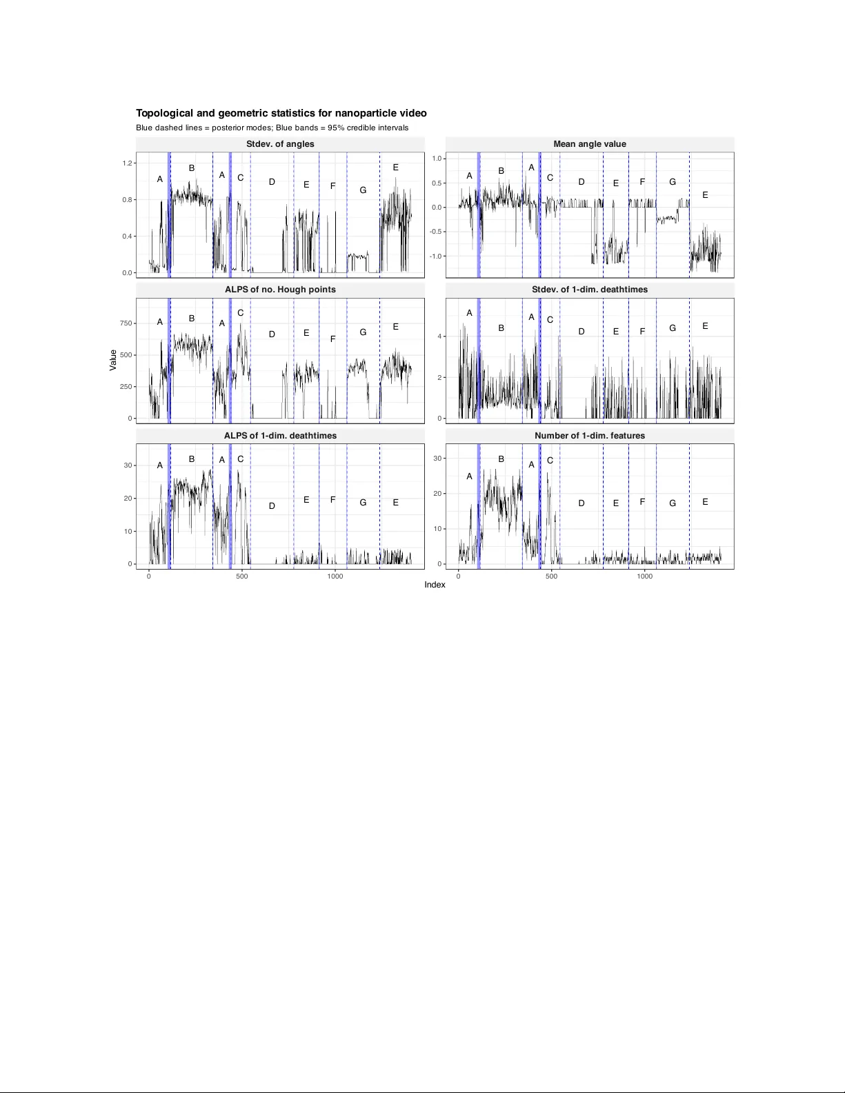
A generalized Ba y esian approac h to m ultiple c hangep oin t analysis Y uh ui W ang 1 , Andrew M. Thomas 2 , and Mic hael Jauc h 1 1 Departmen t of Statistics, Florida State Univ ersit y 2 Departmen t of Statistics and Actuarial Science, Univ ersit y of Io w a Marc h 27, 2026 Abstract W e in tro duce a generalized Ba yesian method for multiple c hangep oin t analysis with a loss function inspired b y m ultinomial logistic regression. The metho d do es not require a sp eciﬁcation of the data-generating pro cess and av oids restrictiv e assump- tions on the nature of c hangep oin ts. F rom the join t p osterior distribution, we can mak e simultaneous inference on the locations of c hangep oin ts and the co eﬃcients of a m ultinomial logistic regression mo del for distinguishing data across homogeneous segmen ts. The m ultinomial logistic regression co eﬃcients pro vide a familiar means of in terpreting p oten tially complex changes. T o select the num b er of changepoints, w e lev erage p osterior summaries that measure whether the m ultinomial logistic classiﬁer can distinguish data from either side of a potential c hangep oint. T o simulate from the generalized p osterior distribution, w e present a Gibbs sampler based on P´ oly a- Gamma data augmentation. W e assess the accuracy and ﬂexibilit y of our method through simulation studies featuring diﬀeren t types of changes and demonstrate its in terpretability through applications to ﬁnancial netw ork data and top ological data deriv ed from nanoparticle videos. Keyw ords: Changep oin t analysis; Generalized Ba yesian inference; Gibbs sampler; Multinomial logistic regression. 1 In tro duction Data collected ov er time often exhibit abrupt structural c hanges. These changes can be complex, esp ecially in mo dern data sets that feature high-dimensional measurements pro- duced by complicated data-generating pro cesses, and their n um b er is t ypically unkno wn. The time indices that partition a heterogeneous series into homogeneous segments are called changepoints. Changep oint analysis is the pro cess of determining the n umber, lo ca- tions, and nature of these c hangep oints. Since the pioneering work of Page ( 1954 ) in the 1 1950s, c hangep oint analysis has b een applied across n umerous disciplines, including ﬁnance ( Banerjee and Guhathakurta , 2020 ), bioinformatics ( Hocking et al. , 2013 ), and climatology ( V erb esselt et al. , 2010 ). There is now a v ast literature on metho ds for c hangep oint anal- ysis. F or a recent review of oﬄine c hangep oint detection, our fo cus in the presen t article, w e refer the reader to T ruong et al. ( 2020 ). The presen t article is motiv ated by three c hallenges that arise in changepoint analysis for mo dern data. First, it can b e challenging to sp ecify a mo del for the data within each homogeneous segmen t. Methods that assume data come from a parametric family (e.g., those describ ed in Chen and Gupta , 2012 ) are lik ely to b e missp eciﬁed in practice, while nonparametric metho ds ma y b e un wieldy or lac k p o wer to detect c hanges. It is diﬃcult to strike the appropriate balance, especially with mo dern data types suc h as images or net works for whic h the data generating pro cess ma y b e quite elab orate. Second, it can b e c hallenging, after identifying a c hangep oin t, to interpret or characterize what exactly c hanged. This c hallenge is comp ounded when the data are higher-dimensional and changes are complex. Third, it can b e c hallenging to prop erly accoun t for uncertain ty across related inferences in c hangep oin t analysis (e.g., inferences regarding the num b er, locations, and nature of the changepoints). T o address these c hallenges, we adopt a generalized Bay esian approach to multiple c hangep oin t analysis, with a loss function inspired by m ultinomial logistic regression. Be- cause the up date from prior to posterior pro ceeds via a loss function rather than a likeli- ho o d function in the generalized Bay esian framew ork, w e av oid the c hallenge of sp ecifying a probability distribution for the data within eac h homogeneous segmen t. W e can also a void making restrictiv e assumptions regarding the nature of changepoints by choosing an appropriate represen tation for the data. F rom the joint p osterior distribution, w e can mak e sim ultaneous inference on the lo cations of changepoints and the co eﬃcien ts of a multino- mial logistic regression mo del for distinguishing data across homogeneous segments. The m ultinomial logistic regression co eﬃcien ts provide a familiar means of in terpreting p oten- tially complex c hanges. The prop osed metho d generalizes the single changepoint metho d of Thomas et al. ( 2025 ) to allo w for sim ultaneous estimation, uncertain ty quan tiﬁcation, and in terpreta- tion of m ultiple c hangep oints. A key comp onent of our metho d is a nov el approach to selecting the n umber of changepoints. In this approach, we ﬁt our generalized Ba y esian m ultiple changepoint method with a ﬁxed but conserv atively large n umber of changepoints and then determine ho w man y of the ﬁtted c hangep oints app ear to corresp ond to true c hangep oin ts b y examining p osterior summaries. This approach provides the user with a p osterior distribution of the n umber of ﬁtted c hangep oin ts that app ear to corresp ond to true changepoints. W e also incorp orate a horsesho e prior ( Carv alho et al. , 2010 ) for the co eﬃcients of the m ultinomial logistic regression, whic h can lead to more eﬃcient and in terpretable estimates when data are higher-dimensional and c hanges o ccur in a small n umber of co ordinates. T o obtain p osterior samples, we construct a Gibbs sampler via P´ oly a-Gamma data augmen tation ( P olson et al. , 2013 ). Finally , w e consider applications to complex data, including a video of a nanoparticle transitioning b etw een ordered and disordered states and dynamic netw ork data that records correlations b et ween sto c k prices 2 o ver time. Sev eral recent articles ha ve exploited classiﬁcation tec hniques for c hangep oin t detection. Londsc hien et al. ( 2023 ) in tro duced a non-parametric method based on a no vel classiﬁer log- lik eliho o d ratio that lev erages probabilistic predictions from a classiﬁer suc h as a random forest. The ClaSP method ( Ermshaus et al. , 2023 ) iden tiﬁes c hange p oin ts b y training a k -nearest neighbor classiﬁer on windo ws before and after prospective c hangep oints, using cross-v alidation to construct a score proﬁle whose peaks indicate potential changes. The metho d changeAUC of Kanrar et al. ( 2025 ) trains a classiﬁer on held-out data from b oth ends of a series and then determines whether and where a c hangep oin t exists by computing the area under the R OC curv e (A UC) of this classiﬁer on each p oten tial split of the data. Our prop osed generalized Bay esian metho d diﬀers from these other metho ds by estimating m ultiple changepoints simultaneously , yielding more interpretable results, and providing uncertain ty quan tiﬁcation regarding the changepoints and related parameters. The remainder of the article is structured as follows. Section 2 brieﬂy reviews the most relev an t bac kground knowledge needed to understand the presentation of our prop osed metho d in Section 3 . In Section 4 , we compare our metho d against several alternativ e metho ds through sim ulation studies. Section 5 presents applications to real data. W e conclude in Section 6 with a summary of our contributions and a discussion of future w ork. 2 Bac kground W e ﬁrst review the generalized Bay esian framework of Bissiri et al. ( 2016 ) and the single c hangep oin t metho d BCLR prop osed b y Thomas et al. ( 2025 ). 2.1 The generalized Ba y esian framew ork T o make inferences regarding an unkno wn parameter θ given data x , a Bay esian approac h uses a lik eliho o d function L ( θ | x ) to up date a prior distribution with density function π ( θ ) to a p osterior distribution with density function π ( θ | x ) ∝ L ( θ | x ) π ( θ ). T o obtain the likelihoo d function, one must sp ecify the data-generating pro cess in the form of a probabilit y distribution. As discussed in Bissiri et al. ( 2016 ), there are scenarios in which this requiremen t can b e prohibitiv ely diﬃcult or unnecessarily cumbersome. The data- generating pro cess ma y be c hallenging to adequately sp ecify , and the resulting lik eliho o d function may b e to o complex to w ork with in practice. The parameter of interest may b e low-dimensional, making inference via a fully sp eciﬁed mo del for the data a burden. Additionally , the parameter of in terest ma y not directly index a family of density functions, presen ting problems for the Ba yesian approach. Bissiri et al. ( 2016 ) established that a v alid, coheren t up date from π ( θ ) to π ( θ | x ) can b e made for parameters which are connected to data x via a loss function ℓ ( θ , x ) rather than a lik eliho o d function by setting π ( θ | x ) = exp {− ℓ ( θ, x ) } π ( θ ) R exp {− ℓ ( θ, x ) } π ( θ )d θ . (1) 3 Dev eloping a changepoint detection metho d under the generalized Bay esian framework will help to mitigate the c hallenges described in Section 1 . In particular, the generalized Ba yesian approach uses a loss function rather than a likelihoo d, a v oiding the need to sp ecify the data-generating pro cess for the data b etw een changepoints. As we will see, the loss function can b e chosen to oﬀer an in terpretable description of the p oten tially complex c hanges o ccurring at eac h c hangep oin t. Finally , the generalized Bay esian approach yields a p osterior distribution that can b e used to quan tify uncertaint y regarding all unknown parameters, as in a standard Ba yesian approac h. The generalized Ba y esian framework has b een applied to other problems closely related to changepoint analysis. F or example, Rigon et al. ( 2023 ) introduced a generalized Ba y esian approac h to probabilistic clustering. In a similar vein, Chakrab ort y et al. ( 2024 ) prop osed a generalized Bay esian approac h to fair clustering, pro viding uncertaint y quan tiﬁcation ab out the optimal clustering conﬁguration while ensuring protected attributes of sub jects are balanced across all clusters. 2.2 A generalized Ba y esian single c hangep oin t metho d W e no w review the single c hangep oint metho d proposed by Thomas et al. ( 2025 ), which w e will refer to as BCLR . This metho d can be understo o d as a special case of the generalize d Ba yesian multiple changepoint metho d we will introduce in Section 3 . Our presen tation is in tended to make the parallels b etw een these metho ds more evident. Let κ ∈ { 1 , . . . , N − 1 } denote a single c hangep oin t dividing a p -dimensional series x 1 , . . . , x N in to tw o homogeneous segmen ts { 1 , . . . , κ } and { κ + 1 , . . . , N } . Let X b e the N × p matrix whose ro ws corresp ond to x 1 , . . . , x N . W e can view BCLR as a generalized Ba yesian metho d with the loss function ℓ ( κ, β , X ) = − log ( κ Y i =1 1 1 + e x ⊤ i β N Y i = κ +1 e x ⊤ i β 1 + e x ⊤ i β ) (2) connecting the parameters of in terest θ = ( κ, β ) to the data X . This loss function is closely related to logistic regression: If the changepoint κ were known, then ( 2 ) would reduce to the negativ e log-lik eliho o d function of a logistic regression mo del for distinguishing b et w een pre- and p ost-changepoint data. The regression co eﬃcien ts allo w one to interpret a changepoint just as one would interpret the co eﬃcients of a logistic regression. The generalized p osterior density satisﬁes π ( κ, β | x 1 , . . . , x N ) ∝ exp {− ℓ ( κ, β , X ) } π ( κ, β ) (3) where π ( κ, β ) is the prior density . As a default setting, Thomas et al. ( 2025 ) c hose a uniform prior for the changepoint and a multiv ariate Gaussian prior for the regression co eﬃcien ts, with the tw o parameters b eing indep enden t a priori . 4 3 Multiple c hangep oin t detection Most real world applications of c hangep oin t analysis feature multiple c hangep oints. Multi- ple c hangep oin t metho ds are often constructed by rep eatedly applying a single changepoint metho d. Common approac hes include binary segmentation and b ottom-up segmen tation ( V ostriko v a , 1981 , F ryzlewicz , 2014 , Zhang and Chen , 2021 , Ross , 2021 , Kork as , 2022 , Ko v´ acs et al. , 2023 ). Binary segmen tation applies a single changepoint metho d recursively b y splitting a series in to tw o segments if a changepoint is found, and then applying the same metho d to eac h of the resulting segmen ts. This pro cess contin ues un til no more c hange- p oin ts are found or a minimum segmen t length is reac hed. Bottom-up segmen tation b egins with a large num b er of p otential c hangep oin ts dividing a series in to numerous segments and then merges neigh b oring segmen ts if there is no evident diﬀerence b etw een them. These approac hes can b e conv enient and eﬀectiv e, but they are not ideal for generalizing the single c hangep oin t approach of Thomas et al. ( 2025 ) b ecause imp ortant adv antages of that metho d, suc h as its interpretabilit y and coherent uncertaint y quan tiﬁcation, would b e lost in the pro cess. Instead, in this section, w e presen t a generalized Bay esian multiple change- p oin t metho d with a loss function inspired by multinomial logistic regression that retains the adv an tages of BCLR by providing simultaneous inference for multiple c hangep oin ts and asso ciated parameters. An imp ortan t comp onent of our metho d is a no vel approac h to selecting the num b er of changepoints based on p osterior summaries. W e also consider a horsesho e prior for the co eﬃcients of the multinomial logistic regression, which can lead to more eﬃcient and in terpretable estimates when data are higher-dimensional and changes o ccur in a small num b er of co ordinates. 3.1 A generalized Ba y esian m ultiple c hangep oin t metho d W e no w supp ose there are L changepoints κ 1 , . . . , κ L ∈ { 1 , . . . , N − 1 } with κ 1 < · · · < κ L that divide the series x 1 , . . . , x N in to J = L + 1 segments. Let κ = ( κ 1 , . . . , κ L ) ⊤ and, for notational conv enience, set κ 0 = 0 and κ L +1 = N . F or each j ∈ { 1 , . . . , L + 1 } , the tw o consecutiv e c hangep oin ts κ j − 1 and κ j deﬁne the j th homogeneous segmen t { κ j − 1 + 1 , . . . , κ j } . Again, let X b e the N × p matrix whose rows corresp ond to x 1 , . . . , x N . Under the generalized Bay esian framew ork, w e c ho ose the loss function ℓ ( κ , β 1 , . . . , β J , X ) = − log ( κ 1 Y i =1 q i 1 · · · N Y i = κ L +1 q iJ ) , where q ij = e x ⊤ i β j P J k =1 e x ⊤ i β k , (4) to connect the parameters of in terest θ = ( κ , β 1 , . . . , β J ) to the data X . This loss func- tion is closely related to multinomial logistic regression. In particular, if the changepoints κ 1 , . . . , κ L w ere kno wn, then ( 4 ) would reduce to the negative log-likelihoo d function of a m ultinomial logistic regression mo del for distinguishing data across homogeneous seg- men ts. In the usual scenario when κ 1 , . . . , κ L and β 1 , . . . , β J are unknown, minimizing the loss function would corresp ond to ﬁnding the com bination of κ 1 , . . . , κ L and β 1 , . . . , β J suc h that the multinomial logistic regression mo del with co eﬃcien ts β 1 , . . . , β J b est discrimi- nates data across homogeneous segments. The regression co eﬃcients can b e interpreted 5 just as we w ould in terpret the co eﬃcien ts of a multinomial logistic regression, providing a familiar wa y of understanding p oten tially complex changes. The generalized Ba yesian p osterior densit y satisﬁes π ( κ , β 1 , . . . , β J | X ) ∝ exp {− ℓ ( κ , β 1 , . . . , β J , X ) } π ( κ , β 1 , . . . , β J ) . (5) Because exp {− ℓ ( κ , β 1 , . . . , β J , X ) } is b ounded ab ov e b y one, a prop er prior distribu- tion leads to a prop er p osterior distribution. By default, w e let π ( κ , β 1 , . . . , β J ) = π ( κ ) π ( β 1 , . . . , β J ) with π ( κ ) ∝  1 κ 1 − κ 0  κ 1 − κ 0  1 κ 2 − κ 1  κ 2 − κ 1 . . .  1 κ L +1 − κ L  κ L +1 − κ L . (6) This prior for κ p enalizes small segmen ts and assigns the greatest mass to the case when all homogeneous segmen ts are of equal length. W e consider tw o diﬀerent prior sp eciﬁcations for the regression co eﬃcien ts. Before describing these, we ﬁrst remark that, as in standard multinomial logistic regression, w e m ust c ho ose a reference class and set the corresponding co eﬃcient v ector to zero. W e let class J b e the reference class and set β J = 0 . When p is small, we assign indep enden t m ultiv ariate Gaussian priors to each of the J − 1 remaining co eﬃcient vectors, with β j ∼ N ( m 0 j , V 0 j ) for each j ∈ { 1 , . . . , J − 1 } . When p is large and we exp ect c hanges to o ccur in only a few dimensions, w e adopt a horsesho e prior ( Carv alho et al. , 2010 ) for β 1 , . . . , β J − 1 . The horsesho e prior has a Gaussian scale mixture representation, with β d j | λ d j , τ ∼ N  0 , λ 2 d j τ 2  , λ d j ∼ C + (0 , 1) , τ ∼ C + (0 , 1) for d = 1 , . . . , p and j = 1 , . . . , J − 1. Here, C + (0 , 1) denotes the half-Cauch y distribution with a lo cation parameter of zero and a scale parameter of one. Each λ d j is a lo cal scale parameter, while τ is the global scale parameter. Since its in tro duction, the horsesho e prior has b een widely adopted as a prior for sparse parameters because of its desirable statistical prop erties and its computational tractabilit y . The horsesho e prior is meant to aggressiv ely shrink estimates to w ard zero when the true co eﬃcien t is zero, but a v oid ov ershrinking estimates of non-zero co eﬃcients. This leads to more eﬃcient and interpretable estimates of sparse parameters. Mak alic and Schmidt ( 2015 ) introduced a simple Gibbs sampler for p osterior inference with the horsesho e prior, lev eraging the fact that the half-Cauch y distribution can b e expressed as a scale mixture of in verse gamma distributions to arrive at a data-augmen ted representa tion of the horsesho e prior. In our context, the data-augmented represen tation is β d j | λ d j , τ ∼ N  0 , λ 2 d j τ 2  , λ 2 d j | ν d j ∼ IG  1 2 , 1 ν d j  , τ 2 | ξ ∼ IG  1 2 , 1 ξ  (7) with ν d j ∼ IG  1 2 , 1  for d = 1 , . . . , p and j = 1 , . . . , J − 1 , and ξ ∼ IG  1 2 , 1  . This represen tation leads to a Gibbs sampler with inv erse gamma full conditional distributions for the lo cal and global scale parameters as well as the newly-in tro duced auxiliary v ariables. 6 W e will refer to this metho d as bcmlr , which is a st ylized acronym for “generalized B a yesian c hangep oint detection with a loss inspired by m ultinomial l ogistic r egression.” Section 3.4 will describ e an approach to selecting the n um b er of changepoints. As with the BCLR metho d of Thomas et al. ( 2025 ), we omit intercept parameters and center the data. W e also standardize the data to facilitate the use of a default prior for the regression co eﬃcien ts when data hav e diﬀeren t scales. 3.2 A Gibbs sampler for m ultiple c hangep oin t detection T o simulate from the p osterior distribution, we apply P´ oly a-Gamma data augmentation to obtain an augmented p osterior density that yields tractable full conditional distributions. F ollowing the Section 6.3 of the supplemen t of Polson et al. ( 2013 ), whic h discusses P´ olya- Gamma data augmen tation for m ultinomial logistic regression, we in tro duce a minor change of notation, re-expressing the loss function ( 4 ) as ℓ ( y , β 1 , . . . , β J | X ) = − log ( N Y i =1 J Y j =1 e η ij y ij 1 + e η ij ) where η ij ( x i , β j ) = x ⊤ i β j − log P k  = j e x ⊤ i β k with y ij = 1 if κ j − 1 < i ≤ κ j and y ij = 0 otherwise. This alternativ e expression for the loss, in tro duced in Held and Holmes ( 2006 ), resem bles the loss function in binomial logistic regression and allows us to lev erage P´ oly a- Gamma data augmentation to obtain the p osterior densit y of ( κ , β 1 , . . . , β J , ω ) , where ω is an N × J matrix of P´ oly a-Gamma auxiliary v ariables. F rom this augmen ted p osterior densit y , w e can deriv e the full conditional distributions necessary to construct a Gibbs sampler. W e will presen t t wo versions of the Gibbs sampler that diﬀer according to the prior distribution assigned to the regression co eﬃcients. In b oth versions, the full conditional distributions of the c hangep oints and the P´ olya-Gamma auxiliary v ariables are the same. F or l ∈ { 1 , . . . , L } , let κ − l denote the collection of all changepoints except for κ l . The full conditional distribution of κ l is a discrete distribution that satisﬁes π ( κ l | κ − l , β 1 , . . . , β J , X ) ∝ π ( κ ) κ l Y i = κ l − 1 +1 q il κ l +1 Y i = κ l +1 q i,l +1 (8) on the supp ort { κ l − 1 + 1 , . . . , κ l +1 − 1 } . The full conditional distribution of ω is the same as in P olson et al. ( 2013 ): ω ij | β 1 , . . . , β J , x i ∼ PG (1 , η ij ) (9) for i ∈ { 1 , . . . , N } and j ∈ { 1 , . . . , J − 1 } . W e ﬁrst present the Gibbs sampler based on Gaussian priors for β 1 , . . . , β J − 1 . F or j ∈ { 1 , . . . , J − 1 } , w e denote by β − j the collection of the remaining J − 2 co eﬃcient v ectors excluding β j . When β j has a Gaussian prior N ( m 0 j , V 0 j ), the full conditional 7 distribution of β j is β j | β − j , ω j , κ , X ∼ N ( m j , V j ) , V j = ( X ⊤ Ω j X + V − 1 0 j ) − 1 , m j = V j  X ⊤ ( Ω j c j + δ j ) + V − 1 0 j m 0 j  , Ω j = diag( ω j ) , ω j = ( ω 1 j , . . . , ω N j ) ⊤ , (10) δ j = y j − 1 N · 1 2 , y j = ( y 1 j , . . . , y N j ) ⊤ (11) c ij = log X k  = j exp  x ⊤ i β k  , c j = ( c 1 j , . . . , c N j ) ⊤ , (12) where j ∈ { 1 , . . . , J − 1 } and i ∈ { 1 , . . . , N } . With Gaussian priors for the regression co eﬃcien ts and the discrete prior distribution ( 6 ) for the changepoints, the Gibbs sam- pler targeting the P´ oly a-Gamma augmented p osterior distribution iterates through the follo wing three steps: κ l | κ − l , β 1 , . . . , β J , X ∼ π ( κ l | κ − l , β 1 , . . . , β J , X ) , ω ij | β j , x i ∼ PG (1 , η ij ) , β j | β − j , ω j , κ , X ∼ N ( m j , V j ) , where l ∈ { 1 , . . . , L } , i ∈ { 1 , . . . , N } , and j ∈ { 1 , . . . , J − 1 } . Next, we describ e the Gibbs sampler that results from assigning the horsesho e prior describ ed in Section 3.1 to the regression co eﬃcients β 1 , . . . , β J − 1 . The data-augmented represen tation of the horsesho e prior in ( 7 ) inv olves additional auxiliary v ariables that m ust b e up dated while Gibbs sampling. The full conditional distribution of β j b ecomes β j | β − j , ω j , κ , X , λ j , ν j , τ , ξ ∼ N ( m j , V j ) , V j = ( X ⊤ Ω j X + Σ 0 j ) − 1 , m j = V j  X ⊤ ( Ω j c j + δ j )  , Σ 0 j = diag  λ 2 1 j τ 2 , . . . , λ 2 pj τ 2  , λ j = ( λ 1 j , . . . , λ pj ) ⊤ , ν j = ( ν 1 j , . . . , ν pj ) ⊤ , where Ω j , c j and δ j remain the same as in ( 10 )-( 12 ). The full conditional distributions of λ d j , ν d j , τ , and ξ are av ailable in Bhattac haryya et al. ( 2022 ). Putting this all together, with the horsesho e prior ( 7 ) for the regression co eﬃcien ts and the discrete prior distribution ( 6 ) for the c hangep oin ts, the Gibbs sampler targeting the augmented p osterior distribution iterates through the following steps: κ l | κ − l , β 1 , . . . , β J , X ∼ π ( κ l | κ − l , β 1 , . . . , β J , X ) , ω ij | β j , x i ∼ PG (1 , η ij ) , β j | β − j , ω j , κ , X , λ j , ν j , τ , ξ ∼ N ( m j , V j ) , λ 2 d j | ν d j , β d j , ξ , λ 2 d j ∼ IG  1 , 1 ν d j + β 2 d j 2 τ 2  , ν d j | λ 2 d j , β d j , ξ , τ 2 ∼ IG 1 , 1 + 1 λ 2 d j ! 8 τ 2 | ν d j , β d j , ξ , λ 2 d j ∼ IG p + 1 2 , 1 ξ + p X d =1 β 2 d j 2 λ 2 d j ! , ξ | τ 2 ∼ IG  1 , 1 + 1 τ 2  , where l ∈ { 1 , . . . , L } , i ∈ { 1 , . . . , N } , and j ∈ { 1 , . . . , J − 1 } . Soft ware implemen ting b oth Gibbs samplers is a v ailable in the ﬁrst author’s GitHub rep ository 1 . In the implemen tation, we emplo y the strategy describ ed in Bhattachary a et al. ( 2016 ) when up dating the regression co eﬃcien ts. As is common practice in the c hangep oin t detection literature, we impose a minim um segmen t length m b etw een con- secutiv e changepoints, whic h mo diﬁes the supp ort of the full conditional distribution ( 8 ). F or simplicit y , w e exclude the minimum segmen t length constraint in ( 8 ). The horsesho e prior can also b e adv antageous in the con text of the single changepoint metho d bclr reviewed in Section 2.2 . W e presen t a simpliﬁed v ersion of the Gibbs sam- pler resulting from the horsesho e prior, sp eciﬁc to the single c hangep oin t setting, in the Supplemen tary Material. 3.3 Initialization and mixing W e hav e found that initializing the Gibbs sampler with ev enly spaced c hangep oints works w ell in most scenarios, and this initialization sc heme was used in the simulation studies of Section 4 as well as the real data applications of Section 5 . F or some v ery challenging conﬁgurations of the true changepoints, how ev er, the Gibbs sampler ma y suﬀer from p o or mixing (e.g., the Marko v chain ma y get stuck in a lo cal mo de and fail to explore the larger space of c hangep oint conﬁgurations). T o address this problem, we considered tw o alternativ e strategies: (1) initializing the Gibbs sampler at c hangep oin t lo cations estimated b y a fast external metho d and (2) applying parallel temp ering ( Geyer , 1991 ). Both of these strategies are av ailable in our softw are implemen tation of bcmlr . In particular, the co de supp orts initialization via kcp ( Arlot et al. , 2019 ), e.divisive ( Matteson and James , 2014 ), and MultiRank ( Lung-Y ut-F ong et al. , 2015 ). Users can also apply the non- rev ersible parallel temp ering metho d of Syed et al. ( 2022 ) as describ ed in the supplementary material. In our exp eriments, initialization via a fast external metho d did not consistently outp erform ev en initialization, and the o ccasional b eneﬁts of parallel temp ering did not out weigh the additional computational burden. Thus, we recommend even initialization as the default choice. 3.4 Determination of the n umber of changepoints Th us far, w e hav e assumed the num b er of changepoints is known. While this is some- times the case, the n umber of c hangep oin ts L true is typically unknown in practice. A natural Ba yesian approach would b e to assign a prior to the num b er of changepoints and then simulate from the resulting p osterior distribution using reversible jump Mark o v chain 1 https://github.com/YuhuiChloe/bcmlr 9 Mon te Carlo ( Green , 1995 ). Ho wev er, this approac h w ould incur a substantial computa- tional cost. W e presen t a computationally tractable alternative that in volv es applying the bcmlr metho d with a conserv ativ e upp er b ound L ﬁtted for the n umber of changepoints and then determining how many of the ﬁtted changepoints corresp ond to true c hangep oin ts b y examining p osterior summaries. W e tak e the p ersp ective that a ﬁtted c hangep oin t corresp onds to a true c hangep oin t if the multinomial logistic regression obtained from our generalized p osterior distribution can classify data on either side of the ﬁtted c hangep oint b etter than a coin ﬂip. F rom this p ersp ective, it is natural to consider whether the area under the R OC curve (A UC) ( Peter- son et al. , 1954 ) of the multinomial logistic regression applied to this binary classiﬁcation task is greater than 0.5, b ecause an AUC less than or equal to 0 . 5 indicates that a classiﬁer is no b etter than a coin ﬂip. More concretely , our approach pro ceeds as follows. W e run the Gibbs sampler in Section 3.2 to obtain ﬁtted changepoints κ ( s ) 1 , . . . , κ ( s ) L ﬁtted from the p osterior densit y ( 5 ). Here, s ∈ { 1 , . . . , S } denotes the iteration num b er. F or eac h iteration s ∈ { 1 , . . . , S } and c hangep oin t l ∈ { 1 , . . . , L ﬁtted } , w e compute an AUC based on data in the tw o neigh- b oring segmen ts on either side of κ l using class lab els y ( s ) i,l +1 and probabilities ˜ q ( s ) i,l +1 . The class lab els are binary with y ( s ) i,l +1 = 0 for i ∈ n κ ( s ) l − 1 + 1 , . . . , κ ( s ) l o and y ( s ) i,l +1 = 1 for i ∈ n κ ( s ) l + 1 , . . . , κ ( s ) l +1 o . The probabilit y ˜ q ( s ) i,l +1 is deﬁned as ˜ q ( s ) i,l +1 = q ( s ) i,l +1 /  q ( s ) i,l +1 + q ( s ) i,l  with q ( s ) i,l +1 and q ( s ) i,l giv en in ( 4 ). This probabilit y can b e understo o d as the conditional probabilit y (according to the m ultinomial logistic regression) of x i b elonging to class l + 1 giv en that x i b elongs to either class l or class l + 1. If the AUC is ab o ve the threshold τ = 0 . 5, we consider κ ( s ) l a true c hangep oint and set an indicator R ( s ) l equal to 1; otherwise, w e do not consider κ ( s ) l a true changepoint and set R ( s ) l = 0. The sum of the indicators L ( s ) true = P L ﬁtted l =1 R ( s ) l is the n umber of ﬁtted c hangep oints that corresp ond to true change- p oin ts in the sense describ ed ab ov e at iteration s. In the end, L (1) true , . . . , L ( S ) true appro ximate the p osterior distribution of the num b er of ﬁtted changepoints that corresp ond to true c hangep oin ts. W e take the posterior mo de of L true as our p oint estimate ˆ L true . In practice, w e recommend a few mo diﬁcations to the approach describ ed ab ov e. Since the AUC estimate calculated ab ov e is based on a p otentially small n umber of observ ations in the tw o neighboring segments, w e recommend computing a (1 − α ) × 100% conﬁdence in terv al for the A UC and using the low er b ound of this interv al instead of the A UC estimate itself. W e use the pROC pac k age ( Robin et al. , 2011 ) to compute A UC estimates and conﬁdence in terv als. T o av oid selecting to o many changepoints due to ov erﬁtting, w e recommend holding out ev ery ζ th observ ation to compute these conﬁdence in terv als while using the remaining data to inform the p osterior distribution of the L ﬁtted c hangep oin ts. One must choose a minimum segment length m greater than ζ to ensure that every segment includes at least one held-out sample. After obtaining an estimate ˆ L true of the num b er of changepoints, w e recommend reapplying the bcmlr metho d to the entire series with L = ˆ L true . This will enable easier in terpretation of the regression co eﬃcients and allow the c hangep oints to o ccur at any lo cation in the series. If there is substan tial uncertain ty 10 regarding the n um b er of ﬁtted c hangep oin ts that corresp ond to true c hangep oin ts (as in, for example, Figure 2 ), the user ma y w ant to reﬁt the bcmlr metho d for eac h of the most probable v alues of L. W e pro vide a function to select the n umber of changepoints in the GitHub rep ository . In that function, all of the mo diﬁcations recommended ab ov e are implemen ted b y default. The approac h describ ed ab ov e includes tw o in terpretable tuning parameters. The tun- ing parameter α (with a default v alue of α = 0 . 05) reﬂects the required lev el of certain ty to determine that a change has o ccurred. The tuning parameter τ (with a default v alue of τ = 0 . 5) determines the magnitude of a c hange necessary for the change to b e detected. 4 Sim ulation studies W e compare the proposed metho d (with the horsesho e prior) to ﬁve non-parameteric meth- o ds: e.divisive ( Matteson and James , 2014 ), kcp ( Arlot et al. , 2019 ), MultiRank ( Lung- Y ut-F ong et al. , 2015 ), ClaSP ( Ermshaus et al. , 2023 ), and changeforest ( Londschien et al. , 2023 ). The latter tw o metho ds, which leverage classiﬁers for changepoint detection, w ere review ed in Section 1 along with changeAUC ( Kanrar et al. , 2025 ). Although Kanrar et al. ( 2025 ) describ ed an extension of their changeAUC metho d to the m ultiple change- p oin t setting, w e found that this extension (with the default n um b er of p erm utations) to ok m uch longer to run than bcmlr and the ﬁv e non-parametric metho ds. F or this reason, we do not include changeAUC in our sim ulation studies. The e.divisive metho d com bines bisection ( V ostriko v a , 1981 ) with a m ultiv ariate divergence measure ( Sz´ ekely and Rizzo , 2005 ) to recursively iden tify changepoints. The kernel-based kcp metho d detects change- p oin ts for data that can b e equipp ed with a positive semideﬁnite kernel. The MultiRank metho d iden tiﬁes segmen t b oundaries b y optimizing a homogeneit y test statistic. Imple- men tation details, including tuning parameters and av ailable pac k ages, for all metho ds in the simulation studies can b e found in the Supplementary Material. W e use the adjusted Rand index ( Morey and Agresti , 1984 ) to assess the accuracy of a c hangep oin t detection metho d. Given a partition of the data based on the true c hangep oin ts and a partition of the data based on estimated changepoints, the Rand index ( Rand , 1971 ) is equal to the prop ortion of the  N 2  pairs of observ ations that are either in the same subset in b oth partitions or in diﬀerent subsets in b oth partitions. The adjusted Rand index (ARI) is the normalized diﬀerence b et ween the Rand index and the exp ected Rand index for a random partition. An ARI of 1 indicates p erfect changepoint estimation. 4.1 Sim ulation scenarios W e ev aluate our metho d and the comp eting metho ds in 12 scenarios that diﬀer based on the t yp e of c hanges (change in mean, change in cov ariance, or c hange in b oth mean and co v ariance), whether the n umber of changepoints is known or estimated, and the dimensionalit y of the data (lo wer-dimensional vs. higher-dimensional). In each scenario, our ev aluation is based on 100 sim ulated series. Each series has length N = 600 and 11 con tains t w o true changepoints, κ 1 = 100 and κ 2 = 500. The data-generating pro cesses are describ ed b elow. Changes in mean (CIM): F or 1 ≤ i ≤ κ 1 and κ 2 + 1 ≤ i ≤ N , we generate x i from the m ultiv ariate Gaussian distribution N ( 0 , I ) where 0 is a p -dimensional v ector of zeros and I is the p × p identit y matrix. F or κ 1 + 1 ≤ i ≤ κ 2 , w e generate x i from the m ultiv ariate Gaussian distribution N ( µ , I ) where the ﬁrst tw o en tries in the mean v ector µ equal 2, the last t wo en tries equal − 2, and the p − 4 en tries in the middle equal 0. W e set p = 14 in the lo wer-dimensional scenario and p = 40 in the higher-dimensional scenario. Changes in cov ariance (CIC): F or 1 ≤ i ≤ κ 1 and κ 2 + 1 ≤ i ≤ N , w e generate x i from N ( 0 , Σ 1 ) . F or κ 1 + 1 ≤ i ≤ κ 2 , we generate x i from N ( 0 , Σ 2 ). In the low er-dimensional scenario, we set p = 4 and let Σ 1 =     1 0 . 8 0 0 0 . 8 1 0 0 0 0 1 0 0 0 0 1     , Σ 2 =     1 0 0 . 8 0 0 1 0 0 0 . 8 0 1 0 0 0 0 1     . In the higher-dimensional scenario, w e set p = 8 . In this case, the diagonal entries of b oth co v ariance matrices Σ 1 and Σ 2 are all equal to one. The (1 , 2) and (2 , 1) entries of Σ 1 are equal to 0 . 9 , but all other oﬀ-diagonal en tries of Σ 1 are equal to zero. The (1 , 3) and (3 , 1) as w ell as (2 , 3) and (3 , 2) entries of Σ 2 are equal to 0 . 9 , but all other oﬀ-diagonal entries of Σ 2 are equal to zero. Changes in mean and cov ariance (CIMC): F or 1 ≤ i ≤ κ 1 , we generate x i from N ( 0 , Σ ) . F or κ 1 + 1 ≤ i ≤ κ 2 , we generate x i from N ( µ , Σ ) . F or κ 2 + 1 ≤ i ≤ N , we generate x i from N ( µ , I ) . In the low er-dimensional scenario, we set p = 4 , let µ b e a p -dimensional vector of ones, and deﬁne Σ =     1 0 . 7 0 0 . 7 0 . 7 1 0 0 0 0 1 0 0 . 7 0 0 1     . In the higher-dimensional scenario, we set p = 8 . W e let the ﬁrst four en tries of µ equal one and the last four entries of µ equal zero. W e deﬁne Σ as follows. The diagonal entries of Σ are all equal to one. The (1 , 2) and (2 , 1) as well as (3 , 4) and (4 , 3) entries of Σ are equal to 0 . 9 , but all other oﬀ-diagonal en tries of Σ are equal to zero. T o detect c hanges in co v ariance, we transform each observ ation in the series using a degree-2 p olynomial feature em b edding ψ : R p → R 2 p + ( p 2 ) that maps x = ( x 1 , . . . , x p ) to ψ ( x ) : =  x 1 , . . . , x p , x 2 1 , . . . , x 2 p , x 1 x 2 , . . . , x 1 x p , x 2 x 3 , . . . , x 2 x p , . . . , x p − 1 x p  . (13) 12 That is, instead of applying our metho d to the series x 1 , . . . , x N , we apply it to the series ψ ( x 1 ) , . . . , ψ ( x N ) . When p = 4 , ψ ( x 1 ) , . . . , ψ ( x N ) ∈ R 14 . When p = 8 , ψ ( x 1 ) , . . . , ψ ( x N ) ∈ R 44 . This transformation step is not necessary for the change in mean scenarios. Each series is cen tered and standardized prior to b eing used in the sim ulation studies to ev aluate the p erformance of eac h metho d. In eac h of the scenarios describ ed ab o ve, c hanges o ccur in relativ ely few dimensions compared to the total num b er of dimensions, motiv ating our c hoice to use the horseshoe prior for the regression co eﬃcients in the bcmlr method. 4.2 Sim ulation results T ables 1 and 2 present the mean ARIs (estimated based on 100 simulated data sets) of the diﬀeren t methods in each of the 12 scenarios outlined ab o ve. The subscripts x and ψ attac hed to the mean ARIs indicate the t yp e of input data, with x corresp onding to the ra w data x i and ψ corresp onding to the degree-2 p olynomial em b edding ψ ( x i ) giv en in ( 13 ). The subscripts attached to the column headings indicate the dimension of the input series. (If the p olynomial embedding is considered for a particular scenario, then the subscript indicates the dimension of ψ ( x i ) rather than the dimension of the raw data x i . ) F or each scenario, the highest mean ARI is b olded, while the lo west mean ARI is underlined. Comparing the mean ARIs when the n umber of changepoints is unknown (T able 1 ), w e observ e the following. F or the tw o CIM scenarios, all metho ds achiev e high mean ARIs ab o v e 0.95, except ClaSP . F or the tw o CIC scenarios (fo cusing on the case of p olynomial em b edded input data), we see that kcp and ClaSP p erformed p o orly (with mean ARIs b elow 0.1 and 0.6, resp ectiv ely), MultiRank and changeforest p erformed b est (with mean ARIs ab o v e 0.9), while bcmlr and e.divisive were in the middle. F or the t w o CIMC scenarios (again, fo cusing on the case of p olynomial em b edded input data), changeforest p erforms b est b y a wide margin (with mean ARIs ab ov e 0.95), while bcmlr is second b est. CIM 14 CIM 40 CIC 14 CIC 44 CIMC 14 CIMC 44 bcmlr 0 . 984 x 0 . 980 x 0 . 804 ψ 0 . 764 ψ 0 . 752 ψ 0 . 630 ψ e.divisive 0 . 987 x 0 . 967 x 0 . 055 x , 0 . 886 ψ 0 . 022 x , 0 . 704 ψ 0 . 538 x , 0 . 535 ψ 0 . 532 x , 0 . 532 ψ kcp 1 . 000 x 1 . 000 x 0 . 088 x , 0 . 095 ψ 0 . 010 x , 0 . 031 ψ 0 . 626 x , 0 . 609 ψ 0 . 555 x , 0 . 560 ψ MultiRank 0 . 989 x 0 . 989 x 0 . 005 x , 0 . 954 ψ 0 . 004 x , 0 . 931 ψ 0 . 536 x , 0 . 741 ψ 0 . 546 x , 0 . 611 ψ ClaSP 0 . 263 x 0 . 287 x 0 . 598 x , 0 . 565 ψ 0 . 526 x , 0 . 497 ψ 0 . 430 x , 0 . 497 ψ 0 . 399 x , 0 . 471 ψ changeforest 0 . 990 x 0 . 984 x 0 . 873 x , 0 . 952 ψ 0 . 574 x , 0 . 953 ψ 0 . 974 x , 0 . 970 ψ 0 . 966 x , 0 . 967 ψ T able 1: Mean ARIs when the num b er of changepoints is unknown. Lo oking at the mean ARIs when the num b er of c hangep oints is kno wn (T able 2 ), w e immediately notice that the mean ARIs are higher than they w ere in the case when the n umber of c hangep oints was unknown, as we should exp ect. F or the tw o CIM scenarios, all metho ds achiev e high mean ARIs ab ov e 0.98, except ClaSP . F or the tw o CIC scenarios (with p olynomial em b edded input data), bcmlr and MultiRank p erform b est (with mean ARIs ab ov e 0.97). F or the t w o CIMC scenarios (with polynomial em b edded input data), MultiRank p erforms b est with bcmlr a close second. The changeforest metho d is ex- 13 cluded from the comparison presented in T able 2 b ecause the av ailable implemen tation do es not allow the user to sp ecify a kno wn n umber of changepoints. CIM 14 CIM 40 CIC 14 CIC 44 CIMC 14 CIMC 44 bcmlr 0 . 998 x 0 . 998 x 0 . 974 ψ 0 . 981 ψ 0 . 944 ψ 0 . 954 ψ e.divisive 0 . 989 x 0 . 989 x 0 . 400 x , 0 . 927 ψ 0 . 325 x , 0 . 878 ψ 0 . 565 x , 0 . 621 ψ 0 . 484 x , 0 . 647 ψ kcp 1 . 000 x 1 . 000 x 0 . 876 x , 0 . 954 ψ 0 . 628 x , 0 . 843 ψ 0 . 906 x , 0 . 881 ψ 0 . 821 x , 0 . 896 ψ MultiRank 1 . 000 x 1 . 000 x 0 . 315 x , 0 . 979 ψ 0 . 309 x , 0 . 981 ψ 0 . 679 x , 0 . 970 ψ 0 . 708 x , 0 . 976 ψ ClaSP 0 . 339 x 0 . 347 x 0 . 806 x , 0 . 777 ψ 0 . 670 x , 0 . 652 ψ 0 . 482 x , 0 . 558 ψ 0 . 461 x , 0 . 510 ψ T able 2: Mean ARIs when the num b er of changepoints is known. In terms of mean ARIs, bcmlr is comp etitive, but not alwa ys the top p erformer. This p erformance is not surprising given that the bcmlr loss function is constructed from a parametric multinomial logistic regression, whereas many of the comp eting metho ds are nonparametric or leverage blac k b ox mac hine learning classiﬁers. Ho w ever, bcmlr pro vides ric h information that go es b eyond p oin t estimates of changepoin t lo cations. The choice of metho d should dep end on the user’s ob jective. If maximizing changepoint estimation accuracy is the primary goal, T able 1 suggests that changeforest may b e the b est choice. If one wan ts changepoint estimation accuracy as well as uncertaint y quantiﬁcation and insigh t in to the c hanges that may hav e o ccured, bcmlr ma y b e preferable. 5 Real data applications In this section, we demonstrate via real data applications that the bcmlr method is well- suited for analyzing subtle changes in complex data. In the Supplementary Material, we also apply bcmlr to annotated data series from V an den Burg and Williams ( 2020 ). These examples serv e as a middle ground b etw een sim ulation studies with kno wn ground truth and our main applications in Sections 5.1 and 5.2 . 5.1 DJIA negativ e correlation netw orks Correlations b et ween stock returns are related to mark et trends ( Longin and Solnik , 2001 ). In particular, correlations increase in bear marke ts suc h as the 2008 ﬁnancial crisis. Kei et al. ( 2025 ) conducted changepoint analysis based on net work data deriv ed from correla- tions among sto ck returns during the 2008 ﬁnancial crisis. In this section, w e re-examine this data with our proposed metho d to illustrate the rich information it provides for change- p oin t analysis and to compare the c hangep oin ts found b y our metho d with those found by Kei et al. ( 2025 ) and the metho ds considered in Section 4 . T o construct adjacency matrices representing netw ork data, Kei et al. ( 2025 ) considered w eekly log returns of 29 sto c ks in the Do w Jones Industrial Average (DJIA) from 2007-01-01 to 2010-01-04, a time frame cov ering the 2008 ﬁnancial crisis. The data are av ailable in the ecp pack age ( James and Matteson , 2015 ). The authors ﬁrst computed sample correlation 14 Homophily T riangles Edges Jun 2007 Dec 2007 Jun 2008 Dec 2008 J un 2009 Dec 2009 0 50 100 150 200 0 100 200 300 0 25 50 75 100 Date Blue dashed lines = posterior modes; Blue bands = 95% credible intervals DJIA network statistics with posterior changepoint modes and CIs Figure 1: The DJIA netw ork statistics with posterior mo de estimates of c hangep oints (blue dashed lines) along with 95% credible in terv als (blue bands) obtained from applying bcmlr . matrices of the log returns for each four-week rolling window. The adjacency matrices w ere constructed from these sample correlation matrices by setting entries equal to one (indicating an edge) if the corresp onding sample correlation w as negative and setting entries equal to zero (indicating no edge) otherwise. This pro cess yielded a series of N = 158 adjacency matrices of dimension 29 × 29 . F or each (undirected) adjacency matrix, Kei et al. ( 2025 ) computed three net work statistics—the num b er of edges, the num b er of triangles, and homophily for risk orientation (see Figure 1 ). T o compute homophily for risk orientation, they ﬁrst assigned lab els to eac h no de (sto c k) based on its cumulativ e no de degree. Sto cks with cumulativ e degrees ab o v e the median cum ulative degree w ere labeled “Hedging-Prone”, while the remaining sto c ks were lab eled “Mark et-F ollowing”. “Hedging-Prone” sto c ks tend to play a defensiv e role relative to mark et dynamics, while “Market-F ollo wing” sto cks align more closely with broader mark et mov ements. Homophily for risk orientation is deﬁned as the num b er of edges whose endp oin ts share the same lab el. This statistic captures the tendency for sto c ks with the same risk orien tation to b e negativ ely correlated with eac h other. Kei et al. ( 2025 ) 15 used these three net work statistics as input data for their method, CPDstergm . T o allo w for comparison, we use the same netw ork statistics as input data for our prop osed metho d and the comp eting methods from the simulation studies in Section 4 . P osterior distribution of the number of fitted changepoint that correspond to true changepoints Number of changepoints P oster ior probability 0.0 0.1 0.2 0.3 0.4 0.001 0.022 0.152 0.304 0.286 0.162 0.061 0.012 0.001 0 0 0 1 2 3 4 5 6 7 8 9 10 Figure 2: The p osterior distribution of the num b er of 10 ﬁtted changepoints that corre- sp ond to true changepoints based on 5000 p osterior samples (after 10000 burn-in samples) obtained from applying the approach in Section 3.4 to select the num b er of c hangep oin ts on the DJIA series. Since the num b er of changepoints L true in the netw ork series is unkno wn, we apply the approac h in Section 3.4 to select the num b er of c hangep oints. W e set L ﬁtted = 10 (this is the upp er bound for L true ), the conﬁdence lev el 1 − α = 0 . 9, the AUC threshold τ = 0 . 5, the minim um segmen t length m = 10, and we hold out every 5th observ ation ( ζ = 5) for A UC calculation. Since the data is low-dimensional, w e use a m ultiv ariate Gaussian N ( 0 , 3 I ) as the prior distribution for the regression co eﬃcien ts. W e center and standardize the net work statistics b efore applying our metho d. W e initialize the c hangep oin ts at ev enly spaced locations along the series and run the Gibbs sampler for T = 15 , 000 iterations, with a burn-in p erio d of T 0 = 10 , 000 iterations. Figure 2 shows a histogram approximating the p osterior distribution of the num b er of ﬁtted changepoints that corresp ond to true c hangep oin ts, in the sense discussed in Section 3.4 . F rom the histogram, w e see that the p osterior distribution do es not concentrate on one v alue, indicating uncertain ty ab out the num b er of ﬁtted cha ngep oin ts that correspond to true changepoints. (In light of this ﬁnding, it is not surprising that some of the other metho ds identify diﬀerent num b ers of changepoints, as shown in T able 3 .) In scenarios lik e this, one may w ant to reﬁt the bcmlr metho d for each of the most probable v alues of L. In this section, how ev er, w e tak e the posterior mo de ˆ L true = 3 as our p oin t estimate of L true and condition all subsequent analysis on the num b er of changepoints b eing equal to three. W e now compare the c hangep oin ts detected by the CPDstergm metho d of Kei et al. ( 2025 ) to those detected b y our prop osed metho d. Kei et al. ( 2025 ) found three c hange- p oin ts corresp onding to the follo wing dates: 2007-04-23, 2008-10-06, and 2009-04-20. The authors link ed these changepoints to three approximately coinciden t even ts: (i) New Cen- 16 Real even t dates bcmlr CPDstergm e.divisive MultiRank (i) 2007-04-02 2007-05-14 2007-04-23 – – (ii) 2008-09-15 2008-09-29 2008-10-06 2008-10-06 2008-09-15 (iii) 2009-03-09 2009-03-23 2009-04-20 2009-04-20 2009-04-06 – – – – 2009-05-18 – – – – 2009-06-29 – – – – 2009-11-16 – – – – 2009-12-28 T able 3: Estimated changepoints from eac h metho d that iden tiﬁed at least one changepoint compared with the dates of real even ts reviewed b y Kei et al. ( 2025 ). tury Financial Corp oration ﬁled for bankruptcy on 2007-04-02, (ii) Lehman Brothers ﬁled for bankruptcy on 2008-09-15, and (iii) the DJIA index b ottomed out on 2009-03-09. The bcmlr metho d, applied to the entire series with L = 3, iden tiﬁes three changepoints corre- sp onding to the follo wing dates: 2007-05-14, 2008-09-29, and 2009-03-23. Compared to the results from CPDstergm , the latter tw o changepoints detected by bcmlr align more closely with the dates of ev ents (ii) and (iii). Figure 1 displa ys the p osterior mo de estimates of the c hangep oin ts (indicated by blue vertical dashed lines) along with 95% credible interv als (indicated b y blue bands). T able 3 sho ws the estimated c hangep oints from eac h metho d that identiﬁed at least one c hangep oint compared to the dates of ev ents (i)-(iii). β 2 − β 1 β 3 − β 2 β 4 − β 3 −5 −4 −3 −2 −1 0 1 2 3 4 −5 −4 −3 −2 −1 0 1 2 3 4 −5 −4 −3 −2 −1 0 1 2 3 4 Edges Triangles Homophily Figure 3: Eac h plot sho ws 95% credible in terv als for diﬀerence β l +1 − β l for l ∈ { 1 , . . . , 3 } . The three dimensions of each diﬀerence v ector relate to edges, triangles, and homophily for risk orien tation. The blac k dots represent p osterior means. W e can interpret whic h co v ariates contributed to each change b y examining p osterior summaries of the regression co eﬃcients, in muc h the same wa y that we would in terpret the co eﬃcien ts of a multinomial logistic regression. The diﬀerence β l +1 − β l is particularly relev an t for interpreting the l th c hangep oint. Figure 3 presen ts p oin t estimates and 95% credible interv als of these diﬀerences for eac h l ∈ { 1 , . . . , 3 } . As an illustration of how 17 1 , …, κ 2 κ 1 + 1 , …, κ 3 κ 2 + 1 , …, N x i T ( β 2 − β 1 ) x i T ( β 3 − β 2 ) x i T ( β 4 − β 3 ) 0 20 40 60 80 20 40 60 80 100 100 110 120 130 140 150 −2.5 0.0 2.5 5.0 Figure 4: Each plot shows p osterior means of x ⊤ i ( β l +1 − β l ), along with 95% p oint wise credible interv als (blue bands), based on the data in neigh b oring segments on either side of the c hangep oint κ l . The blue dashed lines represent the p osterior mo de estimates of the c hangep oin ts. w e can in terpret these diﬀerences, consider the third subplot in Figure 3 , corresp onding to the diﬀerence β 4 − β 3 . W e see that the lo wer b ound of the credible in terv al for the n umber of edges lies ab ov e zero, whereas the credible interv als for the n um b er of trian- gles and homophily for risk orientation b oth include zero. This suggests that the third c hangep oin t corresponds to an increase in the n um b er of edges. An increase in the n um- b er of negatively correlated log returns suggests reduced market risk, whic h aligns with our knowledge that this c hangep oin t o ccurred during the perio d in whic h the DJIA index b ottomed out and b egan to recov er after a 17-mon th b ear mark et. One can in terpret the other changepoints in a similar fashion based on their resp ectiv e subplots. It is also p os- sible to interpret diﬀerences b et ween non-adjacen t segments by examining the diﬀerences b et w een non-consecutive co eﬃcien t vectors. F or example, the diﬀerence β 4 − β 1 con tains information ab out how the the fourth segment diﬀers from the ﬁrst segment. In the multinomial logistic regression mo del implied b y our loss function, the conditional probabilit y that x i b elongs to class l + 1 (i.e. the segment immediately follo wing κ l ) rather than class l (i.e. the segmen t immediately preceding κ l ), given that it b elongs to one of these tw o classes, dep ends on the data through the inner product x ⊤ i ( β l +1 − β l ) . Figure 4 plots the p osterior mean and p oint wise 95% credible interv als of this quan tit y for eac h c hangep oin t. These one-dimensional summaries make it easier to visualize the changes o ccurring at each c hangep oint. As w e alluded to earlier, the comp eting metho ds from the sim ulation studies in Section 4 iden tify a v ariet y of diﬀeren t collections of changepoints when applied to the netw ork statistics. The e.divisive metho d (with the minim um segment length set to 10) detects t wo c hangep oin ts that coincide with the latter t wo c hangep oin t estimates of CPDstergm . The three metho ds kcp (with the maxim um n um b er of changepoints set to 10), ClaSP (with a v alidation classiﬁcation score threshold of 0.75), and changeforest detect no 18 c hangep oin ts. In con trast, MultiRank (with the maxim um num b er of c hangep oin ts set to 10) detects six changepoints, with the ﬁrst t wo o ccurring around even ts (i) and (ii). 5.2 Nanoparticle video In this section, we apply our prop osed metho d to the denoised nanoparticle video app ear- ing in Figure 4 of Crozier et al. ( 2025 ). The authors of that article used top ological data analysis to heuristically characterize nanoparticles into ordered and disordered/unstable states. The v arious b ehaviors of the nanoparticles in ordered states were further c har- acterized by their angular and facial structure. How ever, all of this analysis was done on a frame-by-frame basis b y exp erts. W e will go a step further b y using our prop osed metho d to identify changes in state and characterize these c hanges in a more automated, algorithmic fashion via the estimates of the regression co eﬃcients β 1 , . . . , β J . A distinct adv an tage of the multinomial logistic approach that we pursue here (as opp osed to the binomial logistic approach applied to consecutive segmen ts, as pursued in Thomas et al. , 2025 ) is that it allo ws us to compare the prop erties of a giv en segmen t to those of the other segments. This enables us to b etter understand the b ehavior of our data series within each homogeneous segment. As a heuristic metho d of characterizing the b eha vior in eac h segmen t, we apply k -means clustering to the p osterior mean estimates of β 1 , . . . , β J , selecting the smallest k which pro duces alternating “regimes” (i.e. sequences of frames with similar behavior). Note that, as an extension of our generalized Ba y esian metho d, we could sp ecify a certain num b er of regimes and asso ciate v arious segments to them in an unsup ervised fashion—akin to a hidden Mark ov mo del—but w e lea v e this approac h to future w ork. Before moving on, we en umerate the parameters used when applying our metho d. The n umber of changepoints is unknown, so we set L ﬁtted = 12. F urthermore, w e set the conﬁdence level to 1 − α = 0 . 9, the AUC threshold to τ = 0 . 75, the minim um segment length to m = 30 , and held out every 5th observ ation ( ζ = 5) for A UC computation. F urthermore, we ran the Gibbs sampler for T = 5 , 000 iterations with a burn-in p erio d of T 0 = 2 , 500. The p osterior mo de of the num b er of c hangep oin ts was ˆ L true = 8, which had a p osterior probability of 0 . 649. W e employ ed this v alue as our estimate of L true in this case. T o conduct our analysis of the denoised nanoparticle video dynamics, w e chose a com- bined top ological/geometric feature embedding of statistics. Before analyzing the video, w e smo othed eac h frame in the video according to a Gaussian ﬁlter with σ = 2, binarized it via cross-entrop y thresholding ( Li and Lee , 1993 ), and then remo ved small 8-connected blac k regions in the binary image (of area less than 0.06% of the image size) to reduce noise in our statistics. At this p oint, we summarized our image geometrically by using statistics of the Hough line transform ( Duda and Hart , 1972 ), and top ologically by applying the signed distance ﬁltration to eac h prepro cessed, binarized image ( Garin and T auzin , 2019 ). Sp eciﬁcally , for a white pixel, the signed (Manhattan) distance ﬁltration assigns a pixel in tensity equal to the minimum L 1 distance (minus 1) to a black pixel; for a blac k pixel, it assigns a pixel in tensity equal to the minimum L 1 distance to an y white pixel. W e cal- 19 A B A C D E F G E A B A C D E F G E A B A C D E F G E A B A C D E F G E A B A C D E F G E A B A C D E F G E A L P S o f 1 - d i m . d e a t h t i m e s N u m b e r o f 1 - d i m . f e a t u r e s A L P S o f n o . H o u g h p o i n t s S t d e v . o f 1 - d i m . d e a t h t i m e s S t d e v . o f a n g l e s M e a n a n g l e v a l u e 0 5 0 0 1 0 0 0 0 5 0 0 1 0 0 0 - 1 . 0 - 0 . 5 0 . 0 0 . 5 1 . 0 0 2 4 0 1 0 2 0 3 0 0 . 0 0 . 4 0 . 8 1 . 2 0 2 5 0 5 0 0 7 5 0 0 1 0 2 0 3 0 I n d e x V a l u e B l u e d a sh e d l i n e s = p o st e r i o r m o d e s; B l u e b a n d s = 9 5 % cr e d i b l e i n t e r va l s T o p o l o g i c a l a n d g e o m e t r i c s t a t i s t i c s f o r n a n o p a r t i c l e v i d e o Figure 5: Plot of 6 of the 7 features used to detect nanoparticle activity and tilt in the denoised video from Figure 4 of Crozier et al. ( 2025 ). Blue dashed lines are p osterior modes and blue bands are 95% credible interv als. culated 4 geometric statistics from the Hough transform and 3 top ological statistics. W e c hose indep endent N ( 0 , 3 I ) priors for eac h of the regression co eﬃcien t v ectors. F or the Hough transform statistics, we iden tiﬁed the 8-connected comp onents in the binarized image and applied the Hough transform to each of these individually , thresholding the accumulator in Hough space using a v alue of 150. Using the aggregated p eaks of the Hough line transform from all the connected comp onen ts, we then calculated the standard deviation of the angle v alues of the p eaks (‘Stdev. of angles’ in Figure 5 ); the mean angle of resulting p eaks (‘Mean angle v alue’ in Figure 5 ); the ALPS statistic ( Thomas et al. , 2023 ) of the v alues in the aggregated accumulator arra y (i.e. ‘ALPS of no. Hough points’ in Figure 5 ); and the total num b er of Hough p oints (not depicted in Figure 5 ). These v alues capture a sp eciﬁc crystallographic structure in the nanoparticle bulk which app ears in the images as parallel lines (so-called Mil ler planes ); it also describ es the angles these “lines” take relativ e to the image origin (see righ t ﬁve plots in Figure 6 ). As previously men tioned, we assessed dynamics with topological statistics as well. T o 20 A B A C D E F G E Figure 6: (First ro w) Pixelwise means for each regime iden tiﬁed b y bcmlr . (Second row) Pixelwise standard deviations for eac h regime identiﬁed b y bcmlr . W e can see these cor- resp ond w ell to what is seen in Figure 5 . All of these images are normalized to ha ve mean 1 for ease of comparison. get a ﬁner-grained picture of ho w the nanoparticle evolv es, w e use the signed (Manhattan) distance ﬁltration ( Garin and T auzin , 2019 ). This giv es a b etter idea of the visual size of top ological features than the sublev el set ﬁltration employ ed in Thomas et al. ( 2023 ) and Crozier et al. ( 2025 ). W e aim to describ e the lattice structure via the bright sp ots of the nanoparticle images (cf. top row of Figure 6 ), and w e do so using white regions in the subsequen tly binarized image that are surrounded b y black pixels in the binary image. That is, we use “quadrant IV” features (as detailed in Mo on et al. , 2023 ) and in vestigate their death times—which captures the L 1 radii of the white dots in regimes A, B, C or the L 1 width of the lines 2 in regimes D, E, F, or G . W e calculated the standard deviation of the 1-dimensional death times (‘Stdev. of 1-dim. death times in Figure 5 ); the ALPS statistic of 1-dim. death times (‘ALPS of 1-dim. deathtimes in Figure 5 ); and the num b er of 1-dimensional features in quadrant IV (‘Num b er of 1-dim. features’ in Figure 5 ). Heuristically , these track ed the regularity of the lattice structure and the num b er of “p oin ts” in the lattice (with ALPS b eing a con tinuous measure of the ‘Num b er of 1-dim. features’), resp ectively . In Figure 6 , w e can see that regime A is c haracterized b y a regular hexagonal lattice structure and lo w er ﬂuxionality (particle mo vemen t) compared to regime B , as the second ro w of Figure 6 for regime B is brighter (indicating greater pixelwise v ariance) than that of regime A to the left and righ t (though the size of the atomic features seems more regular in regime B than regime A b y lo oking at the ‘Stdev. of 1-dim deathimes’). Regime C seems to displa y a greater degree of activity at the lo wer surface of the nanoparticle (i.e. the second ro w is brigh ter as we go low er). Regimes D and F are b oth highly ﬂuxional (with nanoparticle structure rarely b eing seen in the video due to rapid mov ement) and ‘Mean angle v alue’ indicates that p erhaps regime D is a little more structured than regime F . Regimes E and G are stable but the particle is oriented at diﬀeren t angles. All of these qualitative nanoparticle conﬁgurations are captured via our summaries, and in an 2 F or example, this captures the “lattice plane separation distance” mentioned in Vincen t and Crozier ( 2021 ). 21 in terpretable manner (as opp osed to a F ourier transform). 6 Discussion W e presented a generalized Ba y esian multiple c hangep oin t metho d with a loss function inspired by multinomial logistic regression. The metho d does not require speciﬁcation of the data-generating pro cess and av oids o v erly restrictive assumptions on the nature of the c hangep oin ts. F rom the joint p osterior distribution, w e can make simultaneous inference on the lo cations of changepoints and the co eﬃcien ts of a multinomial logistic regression for distinguishing data across homogeneous segments. T o select the n um b er of c hangep oin ts, w e introduced an approac h based on p osterior summaries that leverages the multinomial logistic regression mo del implied by the loss function to assess whether data on either side of a p oten tial changepoint can b e reliably distinguished. T o simulate from the generalized p osterior distribution, we constructed a Gibbs sampler via P´ olya-Gamma data augmentation. W e assessed the accuracy of our metho d through simulation studies with diﬀeren t t yp es of c hanges. W e also applied the metho d to netw ork data deriv ed from DJIA sto ck returns and a nanoparticle video. In the nanoparticle video example, we sa w that the prop osed c hange- p oin t metho d, along with a nov el geometric and top ological em b edding, pro vides an eﬀec- tiv e means of characterizing atomic-lev el ﬂuxional b ehavior of nanoparticles in transmission electron microscop y . In the net work data example, we saw that the prop osed metho d oﬀers uncertain ty quantiﬁcation and allows for straigh tforward interpretation of c hangep oin ts. As future w ork, we intend to pursue an extension that can accommo date adjacency ma- trices directly and incorporate appropriate dimension reduction rather than relying up on w ell-chosen netw ork summary statistics. Ac kno wledgemen ts The last author was supp orted b y the National Science F oundation (DMS-2515376). References Arlot, S., Celisse, A., and Harc haoui, Z. (2019). A k ernel m ultiple c hange-p oint algorithm via mo del selection. Journal of Machine L e arning R ese ar ch , 20(162):1–56. Azzalini, A. and Menardi, G. (2014). Clustering via nonparametric density estimation: The R pac k age p dfCluster. Journal of Statistic al Softwar e , 57:1–26. Banerjee, S. and Guhathakurta, K. (2020). Change-p oin t analysis in ﬁnancial net works. Stat , 9(1):e269. Bellman, R. (1954). The theory of dynamic programming. Bul letin of the Americ an Mathematic al So ciety , 60(6):503–515. 22 Bhattac harya, A., Chakrab orty , A., and Mallic k, B. K. (2016). F ast sampling with Gaussian scale-mixture priors in high-dimensional regression. Biometrika , 103(4):985–991. Bhattac haryya, A., Pal, S., Mitra, R., and Rai, S. (2022). Applications of Ba yesian shrink- age prior mo dels in clinical research with categorical responses. BMC Me dic al R ese ar ch Metho dolo gy , 22:126. Bissiri, P . G., Holmes, C. C., and W alker, S. G. (2016). A general framework for updat- ing b elief distributions. Journal of the R oyal Statistic al So ciety: Series B (Statistic al Metho dolo gy) , 78(5):1103–1130. Candanedo, L. M. and F eldheim, V. (2016). Accurate o ccupancy detection of an oﬃce ro om from light, temp erature, h umidit y and CO 2 measuremen ts using statistical learning mo dels. Ener gy and Buildings , 112:28–39. Carv alho, C. M., Polson, N. G., and Scott, J. G. (2010). The horseshoe estimator for sparse signals. Biometrika , 97(2):465–480. Chakrab ort y , A., Bhattachary a, A., and Pati, D. (2024). A Gibbs p osterior framework for fair clustering. Entr opy , 26(1):63. Chen, J. and Gupta, A. K. (2012). Par ametric Statistic al Change Point A nalysis . Birkh¨ auser, Boston, MA, 2nd edition. Crozier, P . A., Leib o vich, M., Haluai, P ., T an, M., Thomas, A. M., Vincent, J., Mohan, S., Morales, A. M., Kulk arni, S. A., Matteson, D. S., W ang, Y., and F ernandez-Granda, C. (2025). Visualizing nanoparticle surface dynamics and instabilities enabled by deep denoising. Scienc e , 387(6737):949–954. Duda, R. O. and Hart, P . E. (1972). Use of the Hough transformation to detect lines and curv es in pictures. Communic ations of the A CM , 15(1):11–15. Ermshaus, A., Sch¨ afer, P ., and Leser, U. (2023). ClaSP: parameter-free time series seg- men tation. Data Mining and Know le dge Disc overy , 37(3):1262–1300. F ryzlewicz, P . (2014). Wild binary segmentation for m ultiple c hange-p oint detection. The A nnals of Statistics , 42(6):2243–2281. Garin, A. and T auzin, G. (2019). A top ological “reading” lesson: Classiﬁcation of MNIST using TD A. In 2019 18th IEEE International Confer enc e on Machine L e arning and Applic ations (ICMLA) , pages 1551–1556. IEEE. Gey er, C. J. (1991). Mark o v chain Mon te Carlo maxim um lik eliho o d. In Computing Scienc e and Statistics: Pr o c e e dings of the 23r d Symp osium on the Interfac e , pages 156– 163, F airfax Station, V A. Interface F oundation of North America. Green, P . J. (1995). Rev ersible jump Mark ov chain Mon te Carlo computation and Bay esian mo del determination. Biometrika , 82(4):711–732. 23 Held, L. and Holmes, C. C. (2006). Bay esian auxiliary v ariable mo dels for binary and m ultinomial regression. Bayesian A nalysis , 1(1):145–168. Ho c king, T. D., Sc hleiermacher, G., Janoueix-Lerosey , I., Bo ev a, V., Capp o, J., Delattre, O., Bach, F., and V ert, J.-P . (2013). Learning smo othing mo dels of copy n umber proﬁles using breakp oint annotations. BMC Bioinformatics , 14:164. James, N. A. and Matteson, D. S. (2015). ecp: An R pack age for nonparametric m ultiple c hange p oint analysis of m ultiv ariate data. Journal of Statistic al Softwar e , 62:1–25. Kanrar, R., Jiang, F., and Cai, Z. (2025). Mo del-free c hange-p oin t detection using A UC of a classiﬁer. Journal of Machine L e arning R ese ar ch , 26(190):1–50. Kei, Y. L., Li, H., Chen, Y., and Madrid P adilla, O. H. (2025). Change p oint detection on a separable mo del for dynamic net works. T r ansactions on Machine L e arning R ese ar ch . Kork as, K. K. (2022). Ensem ble binary segmentation for irregularly spaced data with c hange-p oin ts. Journal of the Kor e an Statistic al So ciety , 51(1):65–86. Ko v´ acs, S., B ¨ uhlmann, P ., Li, H., and Munk, A. (2023). Seeded binary segmen tation: a general metho dology for fast and optimal changepoint detection. Biometrika , 110(1):249– 256. Li, C. H. and Lee, C. K. (1993). Minimum cross en trop y thresholding. Pattern R e c o gnition , 26(4):617–625. Londsc hien, M., B ¨ uhlmann, P ., and Ko v´ acs, S. (2023). Random forests for c hange p oint detection. Journal of Machine L e arning R ese ar ch , 24(216):1–45. Longin, F. and Solnik, B. (2001). Extreme correlation of international equit y mark ets. The Journal of Financ e , 56(2):649–676. Lung-Y ut-F ong, A., L ´ evy-Leduc, C., and Capp ´ e, O. (2015). Homogeneit y and change- p oin t detection tests for m ultiv ariate data using rank statistics. Journal de la So ci´ et ´ e F r an¸ caise de Statistique , 156(4):133–162. Mak alic, E. and Schmidt, D. F. (2015). A simple sampler for the horsesho e estimator. IEEE Signal Pr o c essing L etters , 23(1):179–182. Matteson, D. S. and James, N. A. (2014). A nonparametric approach for multiple c hange p oin t analysis of m ultiv ariate data. Journal of the A meric an Statistic al Asso ciation , 109(505):334–345. Mo on, C., Li, Q., and Xiao, G. (2023). Using p ersisten t homology top ological features to c haracterize medical images: Case studies on lung and brain cancers. The A nnals of Applie d Statistics , 17(3):2192 – 2211. 24 Morey , L. C. and Agresti, A. (1984). The measurement of classiﬁcation agreemen t: An adjustmen t to the Rand statistic for chance agreemen t. Educ ational and Psycholo gic al Me asur ement , 44(1):33–37. Oh, S. M., Rehg, J. M., Balc h, T., and Dellaert, F. (2008). Learning and inferring motion patterns using parametric segmental switching linear dynamic systems. International Journal of Computer Vision , 77(1):103–124. Ok abe, T., Kaw ata, M., Ok amoto, Y., and Mik ami, M. (2001). Replica-exchange Monte Carlo metho d for the isobaric–isothermal ensemble. Chemic al Physics L etters , 335(5– 6):435–439. P age, E. S. (1954). Contin uous inspection sc hemes. Biometrika , 41(1/2):100–115. P edregosa, F., V aro quaux, G., Gramfort, A., Michel, V., Thirion, B., Grisel, O., Blondel, M., Prettenhofer, P ., W eiss, R., Dub ourg, V., et al. (2011). Scikit-learn: Machine Learning in Python. Journal of Machine L e arning R ese ar ch , 12:2825–2830. P eterson, W. W., Birdsall, T. G., and F ox, W. C. (1954). The theory of signal detectability . T r ansactions of the IRE Pr ofessional Gr oup on Information The ory , 4(4):171–212. P olson, N. G., Scott, J. G., and Windle, J. (2013). Bay esian inference for logistic mo dels using P´ olya–Gamma laten t v ariables. Journal of the Americ an Statistic al Asso ciation , 108(504):1339–1349. Rand, W. M. (1971). Ob jectiv e criteria for the ev aluation of clustering metho ds. Journal of the Americ an Statistic al Asso ciation , 66(336):846–850. Rigon, T., Herring, A. H., and Dunson, D. B. (2023). A generalized Ba yes framework for probabilistic clustering. Biometrika , 110(3):559–578. Robin, X., T urck, N., Hainard, A., Tib erti, N., Lisacek, F., Sanchez, J.-C., and M ¨ uller, M. (2011). pROC: an op en-source pack age for R and S+ to analyze and compare R OC curv es. BMC Bioinformatics , 12:77. Ross, G. J. (2021). Nonparametric detection of m ultiple lo cation-scale c hange points via wild binary segmen tation. arXiv pr eprint arXiv:2107.01742 . Sy ed, S., Bouc hard-Cˆ ot´ e, A., Deligiannidis, G., and Doucet, A. (2022). Non-rev ersible parallel temp ering: a scalable highly parallel MCMC scheme. Journal of the R oyal Statistic al So ciety: Series B (Statistic al Metho dolo gy) , 84(2):321–350. Sz ´ ek ely , G. J. and Rizzo, M. L. (2005). Hierarchical clustering via joint b et w een-within distances: Extending W ard’s minim um v ariance metho d. Journal of Classiﬁc ation , 22(2):151–184. 25 Thomas, A. M., Crozier, P . A., Xu, Y., and Matteson, D. S. (2023). F eature detection and hypothesis testing for extremely noisy nanoparticle images using top ological data analysis. T e chnometrics , 65(4):590–603. Thomas, A. M., Jauc h, M., and Matteson, D. S. (2025). Ba yesian c hangep oin t detection via logistic regression and the top ological analysis of image series. T e chnometrics , 67(4):639– 705. T ruong, C., Oudre, L., and V a y atis, N. (2020). Selective review of oﬄine change p oin t detection metho ds. Signal Pr o c essing , 167:107299. V an den Burg, G. J. J. and Williams, C. K. I. (2020). An ev aluation of change p oin t detection algorithms. arXiv pr eprint arXiv:2003.06222 . V erb esselt, J., Hyndman, R. J., Newnham, G., and Culvenor, D. (2010). Detecting trend and seasonal c hanges in satellite image time series. R emote Sensing of Envir onment , 114(1):106–115. Vincen t, J. L. and Crozier, P . A. (2021). A tomic lev el ﬂuxional b eha vior and activit y of CeO 2 -supp orted Pt catalysts for CO o xidation. Natur e Communic ations , 12(1):5789. V ostriko v a, L. Y. (1981). Detecting “disorder” in m ultidimensional random pro cesses. Doklady Akademii Nauk SSSR , 259(2):270–274. Zhang, Y. and Chen, H. (2021). Graph-based multiple change-point detection. arXiv pr eprint arXiv:2110.01170 . 26 Supplemen tary Material for “A generalized Ba y esian approac h to m ultiple c hangep oin t analysis” A Implemen tation details in sim ulation studies This section explains how we obtained the sim ulation results in Section 4.2 of the main article, including ho w we implemented the comp eting metho ds and the prop osed bcmlr metho d in Section 3.1 and computed the adjusted Rand index. Implemen tation of bcmlr . When the num b er of changepoints is kno wn, we estimated the c hangep oin t lo cations b y ﬁtting t wo c hangep oints using the bcmlr Gibbs sampler in Section 3.2 with m = 30. When the num b er of changepoints is unknown, we estimated the n umber and lo cations of c hangep oin ts using the approac h in Section 3.4 with these tuning parameters: τ = 0 . 5, α = 0 . 1, ζ = 5, m = 30, and L ﬁtted = 5. The Gibbs samplers w ere initialized at p ositions that ev enly split the series and run 5 , 000 iterations, with the ﬁrst 2 , 500 discarded as burn-in. Since changes o ccur in relatively few dimensions compared with the total n umber of dimensions based on the data generating pro cesses, w e assigned horsesho e priors for the regression co eﬃcien ts under all scenarios. Implemen tation of kcp and MultiRank . When the n umber of c hangep oin ts is kno wn, the ruptures pac k age ( T ruong et al. , 2020 ) provides functions that implement dynamic programming ( Bellman , 1954 ) to get changepoint estimates from MultiRank and kcp . A radial basis function CostRbf is used for kcp , while a rank-based cost function CostRank is used for MultiRank . F or b oth metho ds, the minimum segment length is set to 30 (same as for bcmlr and e.divisive ). When the num b er of c hangep oin ts is unknown, w e use the functions implementing the “slope heuristics” metho d ( Arlot et al. , 2019 ) av ailable in Londsc hien et al. ( 2023 )’s GitHub simulation rep ository . The implementation of kcp and MultiRank requires sp ecifying a maxim um num b er of c hangep oin ts. W e set the maximum n umber of changepoints equal to 5. Implemen tation of e.divisive . The e.divisive function is implemented in the ecp pac k age ( Matteson and James , 2014 ) and includes an input argumen t k that sp eciﬁes the n umber of c hangep oin ts. When the num b er of changepoints is kno wn, w e set k = 2, in whic h case e.divisive p erforms exactly k bisections to identify k changepoint lo ca- tions. When the num b er of c hangep oin ts is unknown, we do not sp ecify a v alue for k . In this setting, e.divisive recursively bisects the series and, after each bisection, applies a statistical test based on a multiv ariate div ergence measure to assess the signiﬁcance of a changepoint. The implementation of e.divisive also requires sp ecifying a minim um segmen t length. Regardless of whether the n um b er of c hangep oints is kno wn or unkno wn, 27 w e set the minimum segment length to 30, which is the default v alue recommended by Matteson and James ( 2014 ). Implemen tation of ClaSP . The ClaSPy pac k age ( Ermshaus et al. , 2023 ) pro vides the BinaryClaSPSegmentation function for implementing the ClaSP method. Dep ending on whether the n um b er of c hangep oin ts is kno wn, tw o parameters—the n umber of segmen ts and the use of v alidation—are speciﬁed diﬀeren tly . When the n um b er of changepoints is kno wn, we set the n umber of segmen ts equal to 3 and disable v alidation. When the num b er of changepoints is unknown, we do not sp ecify the num b er of segments and instead enable v alidation with a classiﬁcation score threshold of 0.75. These hyperparameter settings are recommended by the authors of ClaSP in their GitHub do cumentation. Implemen tation of changeforest . The changeforest pac k age ( Londschien et al. , 2023 ), a v ailable in both R and Python, pro vides the changeforest function. This func- tion do es not include a parameter for sp ecifying the n um b er of changepoints. In our implemen tation, we set the classiﬁer to a random forest and the searc h metho d to binary segmen tation, whic h are the default settings of the function. Computation of the adjusted Rand index. T o compute the ARI in R, w e used the adj.rand.index function from the pdfCluster pack age ( Azzalini and Menardi , 2014 ). This function tak es as input tw o vectors of equal length, each con taining class lab els cor- resp onding to a particular partition of the data. In the context of c hangep oint detection, these vectors are constructed from the class lab els induced by the true and estimated c hangep oin t lo cations. F or ev aluating c hangep oin t detection metho ds implemen ted in Python, the sklearn.metrics pac k age ( Pedregosa et al. , 2011 ) pro vides a function to compute the ARI, which similarly tak es the true and predicted lab els as inputs. B Additional data applications As mentioned in Section 5 of the main article, we apply bcmlr to m ultiv ariate series with annotations provided by V an den Burg and Williams ( 2020 ). The analysis on the annotated series serv es as a middle ground b etw een sim ulations studies (in Section 4 of the main article) with kno wn ground truth and real data applications without kno wledge of the true changepoints in Section 5 . B.1 Honey b ee dance V an den Burg and Williams ( 2020 ) provided annotations for one of the dance tra jectories of length 609 originally provided b y Oh et al. ( 2008 ). The honey b een dance tra jectory is represen ted b y 4-dimensional vectors: z t = [ x t , y t , sin( θ t ) , cos( θ t )], where x t , y t are the 2D co ordinates, and θ t is the dancer b ee’s heading angle at time t (Figure 7 ). On a v erage, the 28 cos ( θ ) sin ( θ ) y x 0 200 400 600 350 400 450 500 200 250 300 350 −1.0 −0.5 0.0 0.5 1.0 −1.0 −0.5 0.0 0.5 1.0 Time Red dashed = annotated CPs; Blue dashed = posterior modes; Blue bands = 95% credible intervals Honey Bee data with annotated and estimated changepoints Figure 7: A time series representation of a honey b ee dance tra jectory with annotated c hangep oin ts (red dashed lines) and p osterior mo de estimates of changepoints from bcmlr (blue dashed lines). The blue bands are 95% credible interv als. n umber of changepoints annotated was 0.4: F our out of ﬁv e h uman annotators b eliev ed there were no c hangep oints, while one annotator identiﬁed t wo c hangep oints: 182 and 247. Since the true n umber of c hangep oin ts L true is unknown in the honey b ee dance data, w e apply the approac h to selecting the num b er of c hangep oints describ ed in Section 3.4 . Based on the annotator’s low conﬁdence in the presence of changepoints in this series, w e set the n umber of ﬁtted changepoints to L ﬁtted = 4 and choose a conﬁdence level of 1 − α = 0 . 95 for the conﬁdence in terv al for the AUC. In addition, we set the AUC threshold τ = 0 . 5, minim um segmen t length m = 10, and hold out every 5th ( ζ = 5) observ ation for A UC computation. Since the data is relatively low-dimensional, we use a multiv ariate Gaussian distribution N ( 0 , 3 I ) as the prior distribution for the regression co eﬃcien ts. W e center and standardize the series b efore applying our metho d. W e initialize the changepoints at evenly spaced p ositions along the series and run the Gibbs sampler for T = 15 , 000 iterations, with a burn-in p erio d of T 0 = 10 , 000 iterations. W e obtain p osterior samples of the num b er of ﬁtted changepoints that corresp ond to true changepoints, L (1) true , . . . , L (5000) true , 29 and the p osterior mode is ˆ L true = 3. W e reapply the bcmlr metho d on all the data to ﬁt 3 changepoints and ﬁnd that the ﬁrst t wo of the estimated c hangep oints, κ 1 = 175, κ 2 = 244, and κ 3 = 598, closely align with the annotated ones, 182 and 247. Figure 7 presen ts the annotated changepoints (red dashed lines) alongside the estimated changepoint s (blue dashed lines) and 95% credible in terv als (blue bands). β 2 − β 1 β 3 − β 2 β 4 − β 3 −6 −4 −2 0 2 4 6 8 −6 −4 −2 0 2 4 6 8 −6 −4 −2 0 2 4 6 8 x y sin ( θ ) cos ( θ ) Figure 8: Eac h plot shows credible in terv als of the diﬀerences b etw een the co eﬃcien t v ectors β l +1 − β l , for l ∈ { 1 , . . . , 3 } , with 4 dimensions corresp onding to x, y , sin( θ ) and cos( θ ). The blac k dots represen t p osterior mean co eﬃcient v alues. Using p osterior summaries of the co eﬃcients in the m ultinomial logistic regression im- plied b y our loss function, w e can in terpret which cov ariates con tributed to the c hanges. In particular, we can lo ok at 95% credible interv als of β l +1 − β l , the diﬀerences b et ween p osterior co eﬃcien ts that distinguish data in neigh b oring segments on either side of the estimated c hangep oin t κ l (Figure 8 ). W e can interpret the estimated changepoints in the same manner as in Section 5 of the main article. F or example, in the ﬁrst subplot, the credible in terv als corresp onding to sin( θ ), x , and y are in the negative ranges, while the credible interv al corresp onding to cos( θ ) is in the p ositiv e range. Thus, κ 1 = 182 corre- sp onds to the increase of cos( θ ) and the decrease of sin( θ ) , x and y in the honey b ee dance tra jectory . Similarly , the remaining subplots provide insigh t in to what changes occurred around the other detected changepoints. By lo oking at the diﬀerences betw een posterior co eﬃcien ts, we are able to provide in tuitiv e interpretation ab out subtle changepoints in a honey b ee dance tra jectory (Figure 7 ). The comp eting metho ds iden tify diﬀerent changepoints in the honey b ee dance series, while the changepoints detected b y our metho d are closer to the annotated c hangep oin ts. The e.divisive metho d seems to ﬂag noise and ov erestimate the num b er of c hangep oin ts in the honey b ee dance series when the minim um segment length is not chosen care- fully . F or example, e.divisive (with a minimum segment length equal to 10) detects 48 changepoints. Ho wev er, with a minim um segment length to 30, e.divisive detects 15 c hangep oints, lo cated at 42, 87, 119, 174, 204, 235, 269, 299, 333, 363, 402, 440, 472, 30 503, and 558. In contrast, kcp , MultiRank , ClaSP and changeforest are conserv ativ e regarding the existence of c hangep oin ts in this series, whic h aligns with the opinions of most h uman annotators. kcp (with a maxim um num b er of changepoints equal to 4) do es not iden tify a changepoint whereas MultiRank detects one changepoint at 176. Neither ClaSP nor changeforest detects an y changepoints in this series. B.2 Ro om Occupancy Detection This ro om o ccupancy time series (Figure 9 ) is extracted from Candanedo and F eldheim ( 2016 )’s training series at every 16 min utes and has 509 observ ations of light, temp erature, h umidity , and CO 2 . According to V an den Burg and Williams ( 2020 ), all ﬁve human annotators identiﬁed diﬀeren t num b ers of c hangep oints ranging from 2 to 10, yielding an a verage of 6.2 c hangep oints. The most inclusiv e annotation includes 10 c hangep oin ts: 52, 91, 142, 181, 234, 267, 324, 360, 416, 451. Since the true n um b er of changepoints L true is unknown for the ro om o ccupancy data, w e apply the approac h to selecting the n umber of c hangep oin ts described in Section 3.4 . Based on the annotations, w e set the n umber of ﬁtted changepoints to L ﬁtted = 10 and c ho ose a conﬁdence level of 1 − α = 0 . 95 for the conﬁdence in terv al for the AUC. In addition, we set the AUC threshold τ = 0 . 5, minim um segmen t length m = 10, and hold out every 5th ( ζ = 5) for A UC computation. Since the series is relativ ely low-dimensional, w e use a multiv ariate Gaussian distribution N ( 0 , 3 I ) for the regression co eﬃcien ts. W e cen ter and standardize the series b efore applying our metho d. T o initialize the Gibbs sampler, w e position the changepoints at evenly spaced lo cations along the series. W e run the Gibbs sampler for T = 15 , 000 iterations, with a burn-in of T 0 = 10 , 000 iterations. W e obtain p osterior samples of the num b er of ﬁtted c hangep oin ts that corresp ond to true c hangep oin ts, L (1) true , . . . , L (5000) true , and the p osterior mo de is ˆ L true = 10. W e reapply the bcmlr metho d to all the data to ﬁt 10 changepoints and ﬁnd 8 out of 10 of the estimated changepoints closely align with the annotated changepoints. The estimated changepoints are κ 1 = 52, κ 2 = 93, κ 3 = 142, κ 4 = 183, κ 5 = 240, κ 6 = 265, κ 7 = 276, κ 8 = 418, κ 9 = 460, and κ 10 = 498. Figure 9 displa ys the annotated changepoints (red dashed lines) alongside the estimated changepoint s (blue dashed lines) and 95% credible in terv als (blue bands). Using p osterior summaries of the co eﬃcien ts in the multinomial logistic regression implied by our loss function, w e can interpret which co v ariates contributed to the changes. In particular, we lo ok at 95% credible interv als of the diﬀerences b etw een β l +1 − β l , as sho wn in Figure 10 . W e can interpret the estimated changepoints in the same manner as in Section 5 of the main article. F or example, in the ﬁrst subplot, the credible interv als corresp onding to the h umidit y ratio and temp erature are in the p ositiv e ranges, the credible in terv al corresp onding to ligh t lies b elow zero, while the credible interv al corresp onding to CO 2 includes zero. Th us, κ 1 = 52 corresp onds to the increase of the h umidit y ratio and temp erature and the decrease of CO 2 in the ro om. A practical scenario with these c hanges is when p eople leav e the room and turn oﬀ the air conditioning, thereb y heating and h umidifying the room while reducing CO 2 lev els. Similarly , one can in terpret the other 31 Light CO2 HumidityRatio T emperature 0 100 200 300 400 500 19 20 21 22 23 0.003 0.004 0.005 0.006 500 1000 1500 2000 0 200 400 600 Time Red dashed = annotated CPs; Blue dashed = posterior modes; Blue bands = 95% credible intervals Room Occupancy data: series with true and estimated changepoints Figure 9: The ro om o ccupancy time series with annotated changepoints (red dashed lines) and estimated changepoints from bcmlr (blue dashed lines). The blue bands are 95% credible interv als. detected changepoints using the rest of the subplots. Compared with the comp eting metho ds, our metho d pro duces estimated changepoints that are closer to the annotations. The e.divisive and changeforest metho ds seem to ov erestimate the n umber of changepoints, while the kcp and MultiRank metho ds are conserv ativ e ab out the existence of c hangep oints. e.divisive (with a minim um segment length equal to 10) detects 22 changepoints: 12, 54, 64, 92, 102, 143, 153, 170, 182, 192, 240, 258, 268, 340, 351, 369, 411, 421, 441, 460, 470, 480, where half of the estimates are close to the annotations. changeforest detects 59 c hangep oints. kcp (with a maxim um n umber of c hangep oin ts equal to 10) do es not detect an y changepoints, while MultiRank detects 2 c hangep oin ts: 280, 370. ClaSP detects no c hangep oints in this series. 32 β 7 − β 6 β 8 − β 7 β 9 − β 8 β 10 − β 9 β 11 − β 10 β 2 − β 1 β 3 − β 2 β 4 − β 3 β 5 − β 4 β 6 − β 5 −10 −5 0 5 10 −10 −5 0 5 10 −10 −5 0 5 10 −10 −5 0 5 10 −10 −5 0 5 10 temp humid CO 2 light temp humid CO 2 light Figure 10: Each plot shows credible in terv als of the diﬀerences b et ween the co eﬃcient v ectors β l +1 − β l , for l ∈ { 1 , . . . , 10 } , with 4 dimensions corresp onding to temp erature, h umidity ratio, CO2, and light. The blac k dots represen t p osterior mean co eﬃcient v alues. C P arallel temp ering for c hangep oin t detection As mentioned in Section 3.3 , w e can use parallel temp ering to impro v e the mixing of the Gibbs sampler for some very challenging conﬁgurations of the true changepoints. Par- allel temp ering was originally prop osed by Geyer ( 1991 ). Since then, the metho d has b een extended and applied in many ﬁelds to facilitate sampling from multimodal target distributions. T o implement parallel temp ering for our generalized Ba y esian metho d in Section 3.1 , w e need the temp ered v ersions of the posterior densit y in Section 3.1 , Gibbs samplers to sample from the temp ered versions of the augmen ted p osterior densit y , and the acceptance ratio for Metrop olis-Hastings c hecks. First, we raise the exp onen tial term of the negative loss to a temp ering p ow er t ∈ (0 , 1] 33 to get a temp ered version of the p osterior densit y: π t ( κ , β 1 , . . . , β J | X ) ∝ exp {− t · l ( κ , β 1 , . . . , β J , X ) } π ( κ , β 1 , . . . , β J ) , (C.1) where t · l ( κ , β 1 , . . . , β J , X ) = − log    N Y i =1 J Y j =1 e η ij y ij 1 + e η ij ! t    . T o simulate from the temp ered target p osterior density ( C.1 ), we apply P´ olya-Gamma data augmen tation and obtain an augmented p osterior densit y (denoted as π t ) that yields tractable full conditional distributions ( C.2 ), ( C.4 ), and ( C.3 ) as b elo w. ( ω ij | β 1 , . . . , β J , x i ) ∼ PG ( t, η ij ) , for i = 1 , . . . , N ; (C.2) π t ( κ l | κ l − 1 , κ l +1 , B , X ) ∝ l +1 Y j = l α κ j − κ j − 1 j   κ l Y i = κ l − 1 +1 e x ⊤ i β l P J k =1 e x ⊤ i β k κ l +1 Y i = κ l +1 e x ⊤ i β l +1 P J k =1 e x ⊤ i β k   t ; (C.3) ( β j | β − j , ω j , y j , X ) ∼ N ( m j , V j ) , (C.4) where V j = ( X ⊤ Ω j X + Σ − 1 0 j ) − 1 , m j = V j  X ⊤ ( Ω j c j + δ j ) + Σ − 1 0 j µ 0 j  , Ω j = diag( ω j ) , δ j = t  y j − 1 N · 1 2  . These full conditionals are deriv ed under Gaussian priors for regression co eﬃcients β j ∼ N ( µ 0 j , Σ 0 j ) and the segment-length-based prior for changepoints ( 6 ). The comm unication among the chains is determined b y Metrop olis-Hastings chec ks. W e denote the samples from the augmen ted p osterior density as θ t = ( β t , ω t , κ t ). F or tw o temp ering pow ers t 1 , t 2 ∈ (0 , 1] and t 1  = t 2 , the samples θ t 1 and θ t 2 will b e swapped if a random uniform v ariable u ∼ Uniform(0 , 1) is less than min { 1 , A ( t 1 ,t 2 ) } , where A ( t 1 ,t 2 ) = ( π t 1 ev aluated at θ t 2 ) · ( π t 2 ev aluated at θ t 1 ) ( π t 1 ev aluated at θ t 1 ) · ( π t 2 ev aluated at θ t 2 ) . (C.5) Tw o common wa ys to select a pair of samples are the deterministic even-odd (DEO) sc heme ( Ok ab e et al. , 2001 ), where samples with ev en and o dd indices are chosen in an alternating, non-reversible fashion, and the sto chastic even-odd (SEO) sc heme, where samples with ev en and odd indices are c hosen randomly . Sy ed et al. ( 2022 ) sho w ed that DEO outp erforms SEO. 34 T o ac hiev e thorough mixing across mo des using a parallel temp ering algorithm and obtain samples represen tative of the target posterior distribution, it is useful to ﬁnd the optimal temp ering schedule, i.e., the optimal set of temp ering p ow ers. T o ﬁnd the optimal sc hedule, Syed et al. ( 2022 ) prop osed estimating a communication barrier function Λ and solving a minimization problem based on the estimated Λ. A communication barrier at a temp ering pow er t appro ximates the sum of Metropolis-Hastings rejection probabilities from the ﬁrst temp ering p ow er up to t . A lo w v alue of Λ indicates low rejection rates and more active sw aps b etw een the chains at diﬀerent temp ering p o wers. Sy ed et al. ( 2022 )’s non-reversible parallel temp ering method, presen ted in Algorithm 4 of their article, starts with ﬁnding the optimal temp ering schedule. First, they initialize a temp ering schedule. F or a selected n umber of iterations, they p erform steps i) to iii) to estimate the length of the optimal temp ering sc hedule: i) Obtain a list of Metropolis- Hastings rejection probabilities under the DEO sc heme (Algorithm 1). ii) Compute a comm unication barrier ˆ Λ( t ) under every temp ering p o wer t . Estimate a temp ering sched- ule b y ﬁtting a monotone increasing in terp olation ˆ Λ( · ) based on all temp ering p o wers and the corresp onding comm unication barriers (Algorithm 3). iii) Solve optimization problems based on ˆ Λ (Algorithm 2) to obtain the estimated temp ering p ow ers. After iterating these steps to tune the communication barrier and temp ering schedules, the optimal n umber of temp ering p ow ers equals t wice the v alue of the latest communication barrier function ev aluated at temp ering p o wer 1. Then, they apply Algorithm 2 using the latest comm u- nication barrier function and the optimal n umber of temp ering p ow ers to ﬁnd the optimal temp ering schedule. Finally , using Algorithm 1, they obtain p osterior samples from all temp ered versions of the target function under the optimal temp ering sc hedule. T o simulate from our p osterior distribution in Section 3.1 using non-reversible paral- lel temp ering, w e set the temp ered target functions, which are called “lo cal exploration k ernels” b y Syed et al. ( 2022 ), to b e the temp ered p osterior density functions π t ( C.1 ) and use the Gibbs sampler consisting of steps ( C.2 ) to ( C.4 ) to up date p osterior samples. A complete function implementing our metho d with non-reversible parallel temp ering is a v ailable in our GitHub rep ository . D Alternativ e priors for BCLR In the main article, we reviewed Thomas et al. ( 2025 )’s generalized Ba yesian metho d, BCLR , for single c hangep oin t detection, and a Gibbs sampler they constructed under a multiv ariate Gaussian prior for the regression co eﬃcien ts and a uniform prior for the c hangep oint. W e consider diﬀerent priors for the changepoint and the regression co eﬃcients under the BCLR metho d and present another Gibbs sampler for p osterior sim ulation. W e c ho ose a prior for κ based on the lengths of the segmen ts suc h that π ( κ ) ∝  1 κ  κ  1 N − κ  N − κ . (D.1) This choice of prior for κ p enalizes small segments and assigns the greatest mass to the case when the tw o homogeneous segments are of equal length. 35 When the n um b er of co eﬃcients p is small, a m ultiv ariate Gaussian prior is a standard c hoice. When p is large and we exp ect the changes to o ccur in only a few dimensions, w e recommend using the horsesho e prior as in ( 7 ). Giv en the horsesho e prior, the full conditional distribution of β is β | κ, ω , λ , τ ∼ N ( m , V ) , λ = ( λ 1 , . . . , λ p ) V =  X ⊤ Ω X + Σ 0  − 1 , m = V X ⊤ δ , Σ 0 = diag  λ 2 1 τ 2 , . . . , λ 2 p τ 2  , Ω = diag ( ω ) , ω = ( ω 1 , . . . , ω N ) , δ = y − 1 N · 1 2 . The full conditional distributions of the h yp erparameters λ d , ν d , τ and ξ in the horsesho e prior under logistic regression come from Bhattacharyy a et al. ( 2022 ). Based on the discrete prior distribution ( D.1 ) for the changepoint and the horsesho e prior for the regression co eﬃcien ts, the Gibbs sampler that samples from the augmented p osterior distribution under the BCLR metho d iterates through the follo wing steps: κ | β , X ∼ π ( κ | β , X ) , ω i | β , x i ∼ PG  1 , x ⊤ i β  , β | κ, ω , λ , τ ∼ N ( m , V ) , λ 2 d | ν d , β d , ξ , λ 2 d ∼ IG  1 , 1 ν d + β 2 d 2 τ 2  , ν d | λ 2 d , β d , ξ , τ 2 ∼ IG  1 , 1 + 1 λ 2 d  , τ 2 | ν d , β d , ξ , λ 2 d ∼ IG p + 1 2 , 1 ξ + p X d =1 β 2 d 2 λ 2 d ! , ξ | τ 2 ∼ IG  1 , 1 + 1 τ 2  , for d ∈ { 1 , . . . , p } and i ∈ { 1 , . . . , N } . 36

A generalized Bayesian approach to multiple changepoint analysis

Original Paper

Comments & Academic Discussion

Leave a Comment

Original Paper

Related Papers

Comments & Academic Discussion

Leave a Comment