Instance-optimal stochastic convex optimization: Can we improve upon sample-average and robust stochastic approximation?

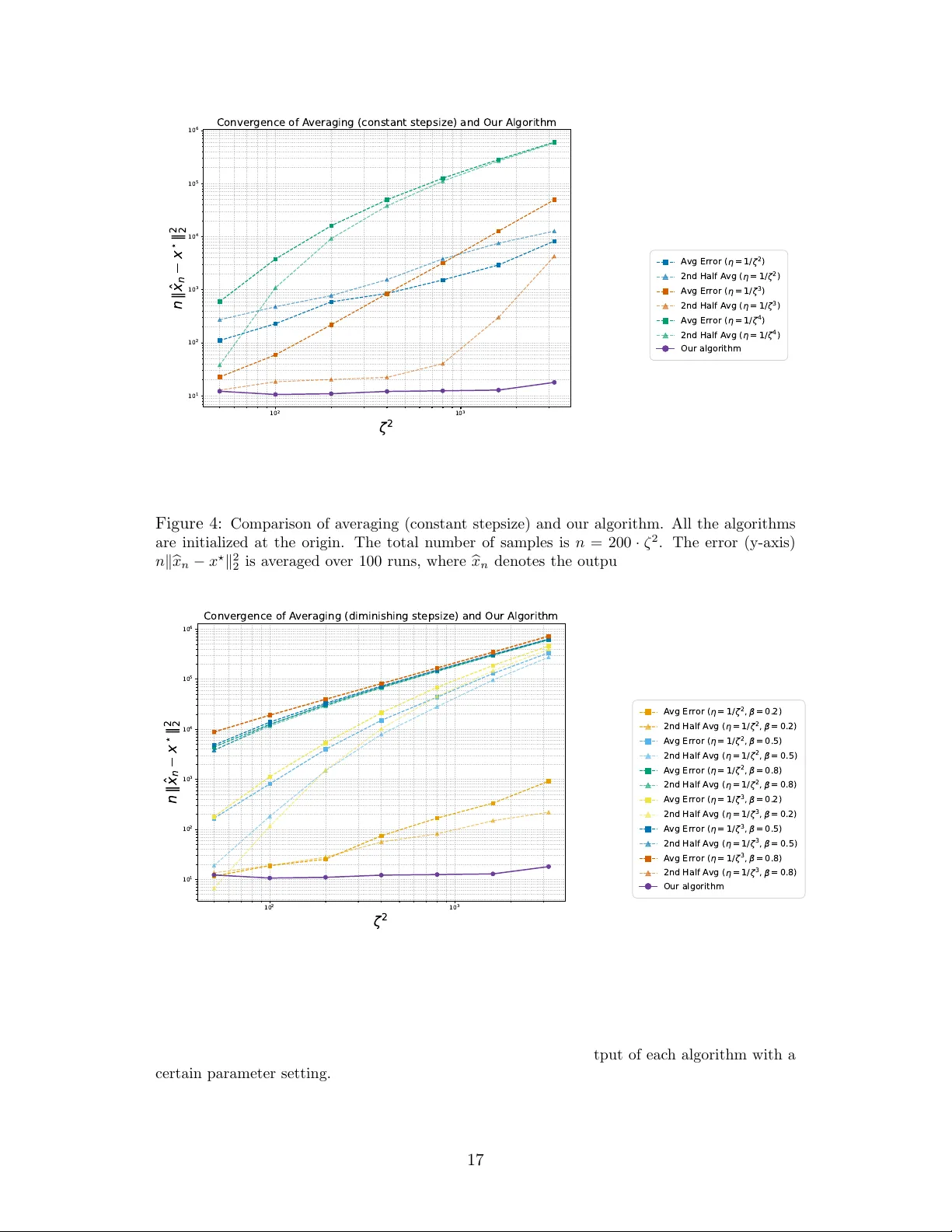
Instance-optimal sto c hastic con v ex optimization: Can w e impro v e up on sample-a v erage and robust sto c hastic appro ximation? Liw ei Jiang ⋆ and Ash win P ananjady † ⋆ Edw ardson Sc hool of Industrial Engineering, Purdue Univ ersity † H. Milton Stew art School of Industrial and Systems Engineering & Sc ho ol of Electrical and Computer Engineering, Georgia Institute of T ec hnology Marc h 27, 2026 Abstract W e study the unconstrained minimization of a smo oth and strongly conv ex p opulation loss function under a sto c hastic oracle that in tro duces b oth additive and multiplicativ e noise; this is a canonical and widely-studied setting that arises across op erations research, signal processing, and mac hine learning. W e b egin by showing that standard approaches such as sample av erage appro ximation and robust (or av eraged) sto chastic approximation can lead to sub optimal — and in some cases arbitrarily p oor — p erformance with realistic ﬁnite sample sizes. In con trast, w e demonstrate that a carefully designed v ariance reduction strategy , which w e term VISOR for short, can signiﬁcan tly outp erform these approac hes while using the same sample size. Our upp er b ounds are complemen ted by ﬁnite-sample, information-theoretic lo cal minimax lo wer b ounds, whic h highligh t fundamen tal, instance-dep endent factors that gov ern the p erformance of an y estimator. T aken together, these results demonstrate that an accelerated v ariant of VISOR is instance-optimal, ac hieving the best p ossible sample complexity up to logarithmic factors while also attaining optimal oracle complexit y . W e apply our theory to generalized linear mo dels and improv e up on classical results. In particular, we obtain the b est-known non-asymptotic, instance-dep enden t generalization error b ounds for sto c hastic methods, ev en in linear regression. 1 In tro duction Consider the canonical sto c hastic optimization problem of minimizing a smo oth and strongly conv ex p opulation ob jective function F f ,P : R d → R , giv en b y F f ,P ( x ) := E z ∼ P [ f ( x, z )] . (1.1) Here we hav e an underlying but unknown distribution P , and f : R d × Z → R is a “sample-wise” ob jective function. Numerous problems in optimization, statistics, and machine learning can b e mo deled as minimizing a population ob jective as in Eq. (1.1), but with access only to n noisy functions { f ( · ; z 1 ) , . . . , f ( · ; z n ) } n i =1 , where z 1 , z 2 , . . . , z n ∈ Z denote i.i.d. observ ations drawn from P . A long line of literature has fo cused on understanding the fundamen tal limits of this problem, and on analyzing ho w the b eha vior of v arious canonical algorithms compares with these limits. Classically , there hav e b een t wo approac hes to this family of questions. The ﬁrst approac h uses the worst-case risk ov er a class of problem instances as the measure b y whic h to compare algorithms and establish low er b ounds [39, 1]. A canonical class of suc h problems (see [14]) is those in whic h the p opulation ob jectiv e is smo oth, µ -strongly con vex, and P art of this w ork w as performed when the ﬁrst author was at Georgia T ec h. 1 the sto c hastic gradients hav e b ounded v ariance at any p oin t: 1 P ( µ, σ ) :=    ( f , P )       F ( y ) − F ( x ) − ⟨∇ F ( x ) , y − x ⟩ ≥ µ 2 ∥ y − x ∥ 2 2 , for an y x, y ∈ R d and E [ ∥∇ f ( x, ξ ) − ∇ F ( x ) ∥ 2 2 ] ≤ σ 2 , for all x ∈ R d    . Then a standard application of F ano’s metho d shows that for any estimator b x n based on i.i.d. samples { z i } n i =1 , we must hav e the worst-case risk low er b ounded as sup ( f ,p ) ∈P ( µ,σ ) E [ ∥ b x n − x ⋆ ( F f ,P ) ∥ 2 2 ] ≥ σ 2 nµ 2 . (1.2) One can ask if the low er b ound (1.2) is achiev ed by an y estimator b x n , and indeed, ov er this class of sto c hastic optimization problems, it is known that minimax rate-optimal estimators can b e constructed with sto c hastic ﬁrst-order information [14]. These estimators ac hieve the worst-case lo wer b ound (1.2) up to universal constan t factors and only require access to ∇ f ( x t , z t ) at carefully c hosen query p oints { x t } n t =1 . On the one hand, the ab o ve results pro vide a complete picture of the worst-case risk in this problem. F urthermore, complexity characterizations based on the minimax risk are w ell-deﬁned for every ﬁnite n and p ossess many app ealing prop erties from the p ersp ectiv e of statistical decision theory [27, 48]. On the other hand, assessing the sample complexit y of algorithms purely in terms of their worst-case risk is p essimistic. Indeed, the w orst-case optimality of an algorithm ov er the global problem class P ( µ, σ ) does not necessarily imply that this algorithm is able to lev erage geometric prop erties of problem instances that are close to ( f , P ). In particular, the worst-case optimalit y of a sto chastic ﬁrst-order metho d do es not imply an ything ab out its adaptivity to any structure present in the instance ( f , P ). As a remedy to the minimax approach, the second approac h to understanding fundamental limits of sto c hastic optimization b etter captures the lo c al desideratum alluded to ab o v e. A typical result of this form, which is a sp ecialization of the one prov ed in [10], tak es the following form: F or a p opulation ob jectiv e F that is smo oth and strongly conv ex with minimizer x ⋆ , deﬁne the Gaussian random vector Z ∼ N   0 , ∇ 2 F ( x ⋆ ) − 1 · co v z i ∼ P ( ∇ f ( x ⋆ , z i )) · ∇ 2 F ( x ⋆ ) − 1 | {z } Λ   . (1.3) Then any estimator b x n based on n i.i.d. samples satisﬁes lim inf c →∞ lim inf n →∞ sup ˜ P : D KL ( ˜ P ∥ P ) ≤ c n E z i iid ∼ ˜ P [ ∥ √ n ( b x n − x ⋆ ) ∥ 2 2 ] ≥ E [ ∥ Z ∥ 2 2 ] = trace (Λ) , (1.4) where D KL ( ·∥· ) denotes the Kullbac k–Leibler (KL) divergence b et ween t wo probability distributions and the limit o ver c is tak en for tec hnical reasons. The lo w er b ound (1.4) implies that in the asymptotic regime when n → ∞ , the estimation error ∥ √ n ( b x n − x ⋆ ) ∥ 2 is b ounded b elo w by trace (Λ), where Λ is the so-called inverse Fisher information matrix , determined by the interaction b et ween the problem’s geometry (captured b y the p opulation Hessian at x ⋆ ) and the noise c haracteristics (captured by the cov ariance of the sample gradient at x ⋆ ). In that sense, this characterization is 1 One can add additional constraints such as Lipschitz contin uit y of gradients and function v alues, but the same information-theoretic minimax low er b ound still holds. 2 instanc e-dep endent , since the error has explicit dep endence on ( f , P ) and may b e small when the instance has fav orable geometry with a small v alue of trace (Λ). As b efore, one can again ask if the low er b ound (1.4) is ac hieved by some estimator b x n . The ﬁrst candidate for suc h an estimator is sample a verage appro ximation (SAA) or empirical risk minimization, which selects an estimator b x ( SAA ) n ∈ argmin x ∈ R d 1 n n X i =1 f ( x, z i ) . Classical results (eg [46, Theorem 3.3]) sho w that under mild regularit y conditions, SAA exhibits asymptotic normality; recalling the matrix Λ from b efore, w e ha ve the weak conv ergence prop ert y √ n ( b x ( SAA ) n − x ⋆ ) w − → Z ∼ N (0 , Λ) . (1.5) Ho wev er, since the ℓ 2 -norm is un b ounded, this do es not imply that the lo wer b ound (1.4) is attained, and SAA can incur inﬁnite ℓ 2 2 risk (see Section 3.2). Having said that, the instance-dep enden t lo w er b ound (1.4) is indeed ac hiev able by a diﬀerent but also classical estimator. Consider the a verage b x ( RPJ ) n = 1 n n X i =1 x k of the iterates { x k } k ≥ 1 of the sto c hastic gradient metho d. Ruppert [45] and Poly ak and Juditsky [44] sho w that with suitable stepsize choices and under mild conditions, this estimator also exhibits asymptotic normality , with √ n ( b x ( RPJ ) n − x ⋆ ) w − → Z ∼ N (0 , Λ) . (1.6) F urthermore, a direct application of [2, Theorem 3] by Bach and Moulines implies that lim n →∞ E z i iid ∼ P [ ∥ √ n ( b x ( RPJ ) n − x ⋆ ) ∥ 2 2 ] → trace (Λ) , (1.7) whic h implies that b x ( RPJ ) n is an asymptotically instance-optimal algorithm for ℓ 2 2 risk. Since the a verage iterate is more numerically stable to hyperparameter c hoices than the last iterate, this metho d is often referred to as r obust sto chastic appr oximation (SA) [38]. 1.1 An illustrative exp eriment: Is optimalit y achiev ed in practice? While the state of aﬀairs describ ed ab o ve suggests that w e ha ve succeeded in dev eloping instance- optimal estimators for sto c hastic optimization, the situation is signiﬁcantly more n uanced in prac- tice. Consider for instance the second notion mentioned ab o ve, of lo cal asymptotic optimalit y . Both the instance-dep enden t low er b ound (1.4) and the upp er b ound (1.7) are v alid only as the sample size tends to inﬁnity , and ma y only b e meaningful for very large (and impractical) n . In practice, w e are in the non-asymptotic or ﬁnite-sample regime, in whic h questions surrounding instance- dep enden t optimalit y ought to take a diﬀerent ﬂav or. Concretely , w e might ask if and when it is p ossible to achiev e an instance-dep endent risk of the order trace (Λ) when n is ﬁnite. In particu- lar, how large must n b e for any algorithm to exhibit such b eha vior, and do es the asymptotically optimal estimator b x ( RPJ ) n p erform w ell in the ﬁnite-sample regime? 3 Figure 1: Heat maps of √ n ( b x ( RPJ ) n − x ⋆ ) for diﬀerent n . W e alwa ys initialize the algorithm at the origin (initial distance to minimizer is √ 2) and eac h heatmap is generated ov er 10 , 000 trials. T o obtain answers to these questions in a concrete example (to be more extensively examined in Section 3.3) consider the follo wing quadratic optimization problem parameterized by ζ ≥ 1. Deﬁne the matrix-vector pair A =  ζ 2 0 0 1  and b =  − ζ 2 − 1  . (1.8) F or this family of ( A, b ) pairs, supp ose our goal is to minimize the function F ( x ) = 1 2 x ⊤ Ax + b ⊤ x using only i.i.d. samples A i of A and b i of b , where • A i = A +  z i − z i − z i z i  and z i are i.i.d. R Vs taking v alues ζ and − ζ with probability 1 / 2 eac h; • b i = b + η i where η i ∼ N  0 0  ,  ζ 4 0 0 1  . A straightforw ard calculation shows that for an y ζ ≥ 1, we ha ve x ⋆ =  1 1  uniformly . Moreo ver, the limiting cov ariance (see Eq. (1.3)) is given b y Λ =  1 0 0 1  uniformly . Therefore, the results discussed ab o ve yield that asymptotically , we ha ve √ n ( b x ( RPJ ) n − x ⋆ ) w − → N  0 0  ,  1 0 0 1  , 4 i.e., the scaled error vector of a veraged stochastic appro ximation conv erges to a standard Gaussian. In Figure 1, w e run simulations of the sto c hastic approximation algorithm in this problem for v arious v alues of n . Even for the moderate c hoice ζ 2 = 20, w e see that the rescaled error √ n ( b x ( RPJ ) n − x ⋆ ) only b egins to resemble a standard Gaussian after appro ximately n = 10 6 samples, whic h is a very large sample size for a 2-dimensional, mo derately-conditioned problem. Before this, the error distribution is skew ed, suggesting a muc h larger ℓ 2 2 error than is predicted asymptotically . T o further prob e this phenomenon, w e run our simulation for a sequence of ζ v alues, choosing a problem-dep enden t sample size n ( ζ ) = 200 ζ 2 for each such simulation. Assuming for the moment that this large a sample size is suﬃcient for some estimator to attain the instance-optimal ℓ 2 2 error, w e should hop e that the rescaled error has distribution resem bling a standard Gaussian. Ho w ever, w e see from Figure 2 that this is not b orne out in practice – the error gets worse as ζ gets larger. Figure 2: Heat maps of √ n ( b x ( RPJ ) n − x ⋆ ) for diﬀerent ζ 2 and sample size n = 200 ζ 2 . W e alw ays initialize the algorithm at the origin (initial distance to minimizer is √ 2) and each heatmap is generated ov er 10 , 000 trials. (Note that x 1 and x 2 ha ve diﬀeren t scales in the ab o ve plots.) This p oor ﬁnite-sample p erformance of the asymptotically optimal estimator b x ( RPJ ) n raises t wo imp ortan t questions: Is p erformance p o or b ecause the giv en problem is information-theoretically c hallenging for our illustrated v alues of n (meaning that no algorithm can signiﬁcan tly impro v e up on the p erformance of b x ( RPJ ) n )? Or is a b etter p erformance attainable in this ﬁnite-sample regime, but b y a diﬀerent estimator? Motiv ated b y these observ ations, w e p ose the follo wing questions for smo oth and strongly conv ex sto c hastic optimization: Q1. How can we characterize the instance-dep enden t hardness of problem (1.1) for a ﬁnite, ﬁxed sample size n ? Q2. Which algorithms can ac hieve optimalit y in this ﬁnite-sample regime? 1.2 Con tributions and organization Our main contribution is to answ er the ab o ve questions. W e pro ve the following results: 1. Non-asymptotic low er b ound and sub optimalit y of b x ( RPJ ) n and b x ( SAA ) n . W e establish a lo wer b ound that c haracterizes the instance-dep enden t hardness of smo oth and strongly con vex sto c hastic optimization problems for any giv en sample size n . W e sho w that, up to a universal constan t factor, the key geometric quan tity that gov erns the lo cal minimax low er b ound in ℓ 2 2 risk is still trace (Λ), as long as the sample size exceeds some explicit, problem-dep enden t threshold n 0 . 5 When applied to the family of quadratic problems ab o v e, our Theorem 6.1 implies that there exist tw o universal constants c 1 and c 2 suc h that for an y sample size n ≤ c 1 ζ 2 , one should not exp ect any reasonable algorithm to attain ﬁnite error. On the other hand, for n ≥ c 1 ζ 2 , the exp ected rescaled ℓ 2 2 error E [ ∥ √ n ( b x n − x ⋆ ) ∥ 2 2 ] is at least c 2 · trace (Λ) = 2 c 2 , where the last equality follows b ecause in this family of problems, we hav e Λ = I . Note that once we ha ve Ω( ζ 2 ) samples, the low er b ound is a universal constant indep endent of ζ . Figure 2, which examines this regime, shows that b x ( RPJ ) n fails to achiev e our non-asymptotic lo wer b ound since the error is sensitive to ζ . Similar issues plague the estimator b x ( SAA ) n . 2. Instance-optimal (and accelerated) sto chastic optimization algorithms. W e prop ose a simple ﬁrst-order online algorithm, VISOR, that incorp orates v ariance reduction techniques wrapp ed around a (p ossibly accelerated) sto chastic approximation inner lo op. F or quadratic optimization problems, VISOR matches our non-asymptotic, instance-dep enden t low er b ound up to a logarithmic factor. F or general non-quadratic problems, it nearly attains the afore- men tioned lo cal lo wer b ound under an additional assumption on the noise in the problem. Since our metho d is in general accelerated, it also achiev es optimal ﬁrst-order oracle complex- it y (whic h is particularly desirable when the noise level is small). Notably , our con vergence guaran tees hold for any norm induced b y an inner pro duct, not only the standard ℓ 2 norm — this feature of our results is not only of general interest but also allo ws to obtain nov el guaran tees on the generalization error of our algorithm for least-squares regression (see the p oin t b elo w). T o illustrate, let us again consider the family of quadratic problems ab o ve, parameterized b y ζ . Applying Theorem 5.2, there exists a universal constant C > 0 such that when the sample size satisﬁes n ≳ log ζ 2 , the output b x n of VISOR satisﬁes E [ ∥ √ n ( b x n − x ⋆ ) ∥ 2 2 ] ≤ C trace (Λ) = 2 C , whic h matches the low er b ound up to a logarithmic factor. Moreov er, as shown in Figure 3, for the same sequence of problems as b efore with sample sizes n = 200 ζ 2 , the rescaled er- Figure 3: Heat maps of √ n ( b x n − x ⋆ ) for our algorithm for diﬀerent ζ 2 and sample size n = 200 ζ 2 . F or each ζ 2 , we alw ays initialize the algorithm at the origin (initial distance to minimizer is √ 2) and p erform 10 , 000 trials to generate the heat map. 6 ror exhibits approximately Gaussian b eha vior with the correct cov ariance structure up to a univ ersal constant factor. Con trast this with the b eha vior of the b x ( RPJ ) n estimator in Figure 2. 3. Applications to generalized linear mo dels. W e apply our conv ergence guarantees to generalized linear mo dels [37] and obtain nearly instance-optimal and non-asymptotic risk b ounds. In particular, we show in Section 5.1.1 that our algorithm improv es the b est kno wn non-asymptotic guaran tees for sto c hastic metho ds in least-squares regression [19] by a factor of the condition num b er. The rest of this paper is organized as follows. Section 1.3 contains a detailed discussion of related work. In Section 2, we set the stage, state key assumptions, and provide concrete examples of problems co v ered by our theory . Section 3 pro vides a non-asymptotic lo cal minimax lo w er b ound for the class of quadratic optimization problems as well as simple examples where b oth SAA and a veraged SGD fail to matc h this low er b ound. W e present our new algorithm in Section 4 and its conv ergence guaran tees in Section 5. Our general non-asymptotic lo wer b ounds are presented in Section 6. Conceptually simple and short pro ofs are presen ted just after the corresponding statemen ts of results, while the more tec hnical pro ofs are deferred to the app endix. 1.3 Related work The literature on statistical analysis in sto c hastic optimization is v ast, and w e cannot hop e to do justice to it here. W e refer the reader to the b o oks [3, 47] for classical (and largely asymptotic) results and the b o ok [26] for a more mo dern non-asymptotic treatment. Belo w, w e discuss the results that are most closely related to the fo cus of our pap er, organized under tw o subheadings. Non-asymptotic instance-dep enden t analysis. Non-asymptotic and instance-dep endent anal- ysis has b een a c hallenging but fruitful program in high-dimensional statistics, and was ﬁrst carried out under the so-called “t w o-p oin t” framew ork b y [4] for estimation of one-dimensional conv ex functions. Unlik e classical minimax analysis that considers the worst-case o ver all functions in a function class, this framework obtains low er b ounds for any sp eciﬁc instance by only considering the w orst-case risk ov er that instance and its hardest alternativ e. While the tw o-p oin t framew ork has b een applied to many diﬀerent contexts since, it is insuﬃcien t to characterize lo cal complexity b ey ond the one-dimensional case. More recently , non-asymptotic and instance-dep enden t guaran- tees ha ve b een established in multiple dimensions with the goal of matc hing the asymptotic risk. Settings considered include Mark ov decision processes [43, 24, 25, 31, 30, 29] and stochastic appro x- imation [32, 18], but these w orks do not justify whether the asymptotic minimax risk remains the appropriate complexity measure in non-asymptotic settings. Non-asymptotic low er b ounds ha ve also b een derived in [34, 33] for estimation in pro jected ﬁxed-p oin t equations and Marko vian linear sto c hastic approximation. How ever, b oth settings are linear and do not address nonlinear scenarios that form the fo cus of our work. Lo cal guarantees for sto chastic optimization. As men tioned in Section 1, the pap er [10] applied H´ ajek and Le Cam’s lo cal minimax theory to develop asymptotic local minimax low er b ounds for stochastic optimization problems. This asymptotic complexity measure is matc hed b y the Rupp ert–Poly ak–Juditsky av eraging pro cedure exactly in smo oth [45, 44], nonsmo oth and constrained settings [7]. Recent work [23] studies general sto c hastic constrained conv ex optimization problems and prop oses a non-asymptotic instance-dep endent lo wer b ound that is extracted from the proof of the asymptotic lo cal minimax theory . Ho wev er, it is unclear whether the hardest instances asymptotically are also the hardest instances for each ﬁxed sample size. Also inspired 7 b y non-asymptotic b ounds, the pap er [54] applies the t wo-point low er b ound to sto c hastic conv ex optimization, characterizing problem diﬃculty in one-dimensional problems. A recen t eﬀort to capture lo cal geometry in optimization problems was also made in the pap er [6]. More broadly , non-asymptotic guarantees for sto c hastic optimization problems hav e b een stud- ied extensiv ely in the literature, and w e pro vide a brief ov erview of results under smo oth and strongly conv ex settings. The optimal algorithm in the classical minimax sense has b een studied in [14, 15], where Ghadimi and Lan prop ose the A C-SA algorithm and sho w that its restarted version is worst-case optimal under the assumption that gradien t noise has uniformly b ounded v ariance. Mo ving beyond worst-case characterizations, instance-dep endent analysis of stochastic optimization algorithms has also b een carried out in several works. The work [41] prov es an instance-dep enden t rate for iterate con vergence of stochastic gradien t descent (SGD), but the rate itself is not instance- optimal. Applying v ariance-reduction tec hniques, the pap er [42] pro ves an instance-optimal rate on the gradien t norm, but it is unclear how the analysis can b e extended to iterate conv ergence without losing instance-optimalit y . The works [2], [53], and [13] provide non-asymptotic analysis for Ruppert–Poly ak–Juditsky a veraging and the con v ergence rate of has an instance-dep enden t leading term that matches the asymptotically optimal rate, and with higher-order term (whic h con trols non-asymptotic p erformance) taking the form O ( n − 7 / 6 ) in the ﬁrst w ork and O ( n − 5 / 4 ) in the last t wo works. The w ork [28] prop oses the R OOT-SGD algorithm and provides conv ergence guaran tees in terms of gradien t norm, distance to solution, and function gap. All the con vergence rates ha ve leading terms that match the asymptotically optimal rate, and higher-order terms scale as O ( n − 3 / 2 ), impro ving up on early w orks. The paper [12] prop oses streaming SVR G and sho ws that under a self-concordance assumption, its con vergence rate on the function gap has a leading term that can b e made arbitrarily close to the asymptotic rate of empirical risk minimization. How ev er, in all the works ab o ve, the conv ergence rates hav e higher-order terms that can b e p oten tially muc h larger than the leading term, and the num b er of samples they require for the higher-order terms to b e dominated by the optimal leading term can b e large (as illustrated in Figure 1). Besides these pap ers, an extensiv e b o dy of work [8, 9, 20, 19] studies and obtains instance- dep enden t guaran tees for least-squares regression, which is an important special case of our setting. In particular, [19] obtains the b est-kno wn sample complexit y for sto c hastic metho ds. As alluded to b efore, many of these algorithms rely on careful forms of v ariance reduction. Our algorithm also dra ws inspiration from SVR G [22] but makes crucial mo diﬁcations to it. F or a review of related w orks on v ariance-reduced gradient metho ds, we refer the reader to a recen t survey pap er [17]. 1.4 Notation Let ⟨· , ·⟩ denote the dot pro duct in Euclidean space, which induces norm ∥ x ∥ 2 = p ⟨ x, x ⟩ . F or r > 0 and x ∈ R d , w e denote by B r ( x ) and B r ( x ) the op en and closed Euclidean balls of radius r cen tered at x , respectively . W e denote the unit sphere in R d under the standard Euclidean norm b y S d − 1 . As previously mentioned, we will w ork not just with the ℓ 2 norm but with general Hilb ert norms 2 ∥ · ∥ . Since w e op erate in ﬁnite-dimensional spaces, any such norm can b e written as ∥ x ∥ = ∥ x ∥ Q := p ⟨ x, Qx ⟩ for some p ositiv e deﬁnite matrix Q . W e denote the dual of the norm ∥ · ∥ by ∥ · ∥ ∗ , i.e. ∥ y ∥ ∗ = sup ∥ x ∥≤ 1 ⟨ x, y ⟩ . F or any matrix M ∈ R d × d , we use ∥ M ∥ to denote the induced op erator norm, i.e., ∥ M ∥ = sup ∥ x ∥ =1 ∥ M x ∥ . In particular, ∥ A ∥ 2 will denote the spectral norm of a matrix A . The notation ∥ A ∥ nuc denotes the nuclear norm of A , namely , the sum of all its singular v alues. F or an y matrix A ∈ R d × d , we let det( A ) denote the determinan t of A . F or a symmetric matrix A ∈ R d × d , w e use λ max ( A ) and λ min ( A ) to denote its largest and smallest 2 Ev en when w e work with general norms, the inner pro duct will alwa ys denote the Euclidean dot product. 8 eigen v alue, resp ectiv ely . F or symmetric matrices A, B ∈ R d × d , w e write A ⪯ B if B − A is p ositive semideﬁnite, and A ⪰ B if B ⪯ A . F or a random vector ξ with b ounded second momen t, we denote its cov ariance matrix by cov( ξ ) = E [( ξ − E [ ξ ])( ξ − E [ ξ ]) ⊤ ]. A random v ariable X is sub-exp onential with parameters ( ν 2 , α ) if for an y t such that | t | ≤ 1 α , we hav e E [ e t ( X − E [ X ]) ] ≤ e t 2 ν 2 2 . Deﬁne the Orlicz norms ∥ X ∥ ψ 1 := inf  t > 0     E  exp  | X | t  ≤ 2  and ∥ X ∥ ψ 2 := inf  t > 0     E  exp  X 2 t 2  ≤ 2  . It is w ell-kno wn that X is sub-exp onential iﬀ ∥ X ∥ ψ 1 < ∞ . W e sa y X is sub-Gaussian if ∥ X ∥ ψ 2 < ∞ . F or any con tinuously diﬀeren tiable function h : R d → R , we let ∇ h ( x ) ∈ R d denote the gradient of h ev aluated at x . When h is twice diﬀeren tiable, we denote its Hessian at x ∈ R d b y ∇ 2 h ( x ) ∈ R d × d . F or a general smo oth map G : R d → R m , w e denote its Jacobian at x ∈ R d b y ∇ G ( x ) ∈ R m × d , whic h can also b e view ed as a linear map from R d to R m . F or tw o maps F and G , we write F ≡ G if they are identical. F or t wo sequences of nonnegative reals { f n } n ≥ 1 and { g n } n ≥ 1 , we use f n ≲ g n to indicate that there is a universal p ositiv e constant C such that f n ≤ C g n for all n ≥ 1. W e use f n ≲ log g n to indicate that there is a universal p ositiv e constant c such that f n ≲ g n log c ( en ). The relation f n ≳ g n (resp. f n ≳ log g n ) indicates that g n ≲ f n (resp. g n ≲ log f n ). W e also use the standard order notation f n = O ( g n ) to indicate that f n ≲ g n and f n = ˜ O ( g n ) to indicate that f n ≲ log g n . W e say that f n = Ω( g n ) (resp. f n = ˜ Ω( g n )) if g n = O ( f n ) (resp. g n = ˜ O ( f n )). F or any x ∈ R , ⌈ x ⌉ and ⌊ x ⌋ denote the smallest integer greater than or equal to x and the largest integer less than or equal to x , resp ectively . 2 F ormal setup and examples In referring to the p opulation ob jectiv e F f ,P in Eq. (1.1), we drop the subscripts ( f , P ) when these are clear from context. W e denote the minimizer of F b y x ⋆ ( F ) if it is unique, and drop the paren theses when F is clear from context. When it is not clear if there is a unique minimizer, w e use argmin F to denote the set of minimizers. F or the sample-wise functions, we use ∇ f ( · , z ) to denote the gradient of f with resp ect to its ﬁrst argument whenev er this is well-deﬁned. Recall that a function h is µ -strongly conv ex and L -smo oth with resp ect to a norm ∥ · ∥ if h is diﬀeren tiable and µ 2 ∥ y − x ∥ 2 ≤ h ( y ) − h ( x ) − ⟨∇ h ( x ) , y − x ⟩ ≤ L 2 ∥ y − x ∥ 2 for all x, y in its domain. W e fo cus on the smo oth and strongly con vex setting and b egin with the follo wing assumption on the p opulation ob jective function. Assumption A. The p opulation obje ctive function F is µ -str ongly c onvex and L -smo oth on R d with r esp e ct to the norm ∥ · ∥ . We denote its minimizer by x ⋆ . A dditional ly, F has L H -Lipschitz Hessian in an instanc e-sp e ciﬁc norm, me aning that for any x, x ′ ∈ R d , ∥∇ 2 F ( x ⋆ ) − 1 ( ∇ 2 F ( x ) − ∇ 2 F ( x ′ )) ∥ ≤ L H ∥ x − x ′ ∥ . (2.1) We further deﬁne ω := inf ∥ v ∥ =1 ∥∇ 2 F ( x ⋆ ) v ∥ ∗ , so that ∥∇ 2 F ( x ⋆ ) v ∥ ∗ ≥ ω ∥ v ∥ for any v ∈ R d . 9 Note that the Lipsc hitz Hessian condition (2.1) is stated with resp ect to a norm scaled by ∇ 2 F ( x ⋆ ) − 1 . This instance-dep enden t condition naturally reﬂects the lo cal geometry at the optimal solution: directions asso ciated with larger curv ature at x ⋆ allo w for greater v ariations in the Hessian. Note also that ω ≥ µ (see Lemma D.1). Next, we state our regularity condition on the sto c hastic noise. Assumption B. F or every ﬁxe d sample z , the function f ( · , z ) is diﬀer entiable. The sto chastic gr adient ∇ f ( x, z ) has a ﬁnite se c ond moment for al l x ∈ R d . Mor e over, ther e exists a c onstant ζ ≥ 0 such that, for al l x, x ′ ∈ R d , E z ∼ P h   ( ∇ f ( x, z ) − ∇ F ( x )) − ( ∇ f ( x ′ , z ) − ∇ F ( x ′ ))   2 ∗ i ≤ ζ 2 ∥ x − x ′ ∥ 2 , (2.2) wher e F ( x ) := E z ∼ P [ f ( x, z )] . We denote the c ovarianc e matrix of the sto chastic gr adient at the optimum by Σ := co v z ∼ P ( ∇ f ( x ⋆ , z )) . Assumption B has app eared in [28] in the optimization setting and in [33, 31] in other related settings. W e point out that our assumption do es not require that each sample ob jective is L -smooth and it is strictly weak er than the following p opular assumption in sto c hastic optimization (e.g. the pap ers [2, 36, 12, 41, 23], which use this stronger assumption with ∥ · ∥ = ∥ · ∥ 2 ): Assumption B ' . F or almost every z , the function f ( · , z ) is diﬀer entiable. The noisy gr adient ∇ f ( x, z ) has ﬁnite se c ond moment for any x ∈ R d . In addition, ther e exists ζ ′ ≥ 0 such that for any x, x ′ ∈ R d : ∥∇ f ( x, z ) − ∇ f ( x ′ , z ) ∥ ∗ ≤ ζ ′ ∥ x − x ′ ∥ almost sur ely. (2.3) It is straightforw ard to verify that the almost sure Lipsc hitz gradient assumption (2.3) implies that Assumption B holds with ζ = 2 ζ ′ . W e now presen t some examples in whic h Assumptions A and B hold. Example 1: Quadratic optimization. Suppose that w e w ant to optimize the function F ( x ) = 1 2 x ⊤ Ax + b ⊤ x, where A ∈ R d × d is symmetric p ositiv e deﬁnite and b ∈ R d is a constant v ector. Instead of accessing A and b directly , w e only observe i.i.d. samples ( A i , b i ) ∼ P suc h that E [ A i ] = A and E [ b i ] = b. W e can deﬁne the sample ob jective function f ( x, ˜ A, ˜ b ) = 1 2 x ⊤ ˜ Ax + ˜ b ⊤ x and mo del the task as a sto c hastic optimization problem. When ∥ · ∥ is the ℓ 2 norm, it is straigh tforward to verify that Assumption A holds with µ = λ min ( A ), L = λ max ( A ), and L H = 0. On the other hand, when ∥ · ∥ = ∥ · ∥ A is induced by the Hessian matrix A , we see that Assumption A holds with µ = L = 1 and L H = 0. In general, Assumption B holds with parameter ζ if A i is symmetric, A i x + b i has ﬁnite second momen t for any x ∈ R d and sup ∥ v ∥ =1 E [ ∥ ( A i − A ) v ∥ 2 ∗ ] ≤ ζ 2 . In Section 3, we will pa y particular atten tion to this family of problems since p opular algorithms already exhibit sub optimalit y on such simple instances. ♣ 10 Example 2: Least-squares regression. Consider the follo wing problem min x ∈ R d F ( x ) , where F ( x ) = 1 2 · E ( ξ ,y ) ∼ P [( y − ⟨ x, ξ ⟩ ) 2 ] . Here, the sample ob jective function for a giv en ( ξ , y ) is f ( x, ξ , y ) = 1 2 ( y − ⟨ x, ξ ⟩ ) 2 . Let H denote the second moment matrix of ξ , which is also the Hessian of F , i.e., H = E ( ξ ,y ) ∼ P [ ξ ξ ⊤ ] = ∇ 2 F ( x ). Supp ose that H ≻ 0 and that each co ordinate of ξ has ﬁnite second and fourth moments. These assumptions are standard and also app ear in the literature [19, Section 2.1]. Since H is p ositiv e deﬁnite, F is a strongly conv ex quadratic function, and we denote its unique minimizer by x ⋆ . F or a sample ( ξ , y ) ∼ P , w e denote the noise as ϵ = y − ⟨ ξ , x ⋆ ⟩ . By the optimalit y conditions at x ⋆ , we hav e E [ ϵξ ] = 0 and Σ = co v ( ξ ,y ) ∼ P ( ∇ f ( x ⋆ , ξ , y )) = E [ ϵ 2 ξ ξ ⊤ ] . Deﬁne the statistical condition num b er ˜ κ as the smallest non-negative num b er such that E [ ∥ ξ ∥ 2 H − 1 ξ ξ ⊤ ] ⪯ ˜ κH . (2.4) No w consider the case that ∥ · ∥ is induced by the Hessian matrix H . Then it can b e v eriﬁed that Assumption A holds with µ = L = 1 and L H = 0. Moreov er, for any x, x ′ ∈ R d , we hav e E [ ∥∇ f ( x, ξ , y ) − ∇ f ( x ′ , ξ , y ) ∥ 2 ∗ ] = E [ ∥∇ f ( x, ξ , y ) − ∇ f ( x ′ , ξ , y ) ∥ 2 H − 1 ] = E [ ∥  x − x ′ , ξ  ξ ∥ 2 H − 1 ] = ( x − x ′ ) ⊤ E [ ∥ ξ ∥ 2 H − 1 ξ ξ ⊤ ]( x − x ′ ) ≤ ˜ κ ∥ x − x ′ ∥ 2 H . Therefore, Assumption B holds with ζ 2 = ˜ κ . ♣ Example 3: Regularized GLM. Let ( ξ i , y i ) ∈ R d × Y b e i.i.d. samples from a joint distribution P giv en b y a generalized linear mo del (GLM). In particular, assume y i | ξ i follo ws an exp onen tial- family distribution with natural (canonical) parameter θ i and disp ersion r ( ϕ ) > 0: p ( y i | θ i ) = exp  y i θ i − u ( θ i ) r ( ϕ ) + s ( y i , ϕ )  . With the c anonic al link , the linear predictor equals the natural parameter, i.e., θ i = ⟨ x, ξ i ⟩ . Note that − log p ( y i | θ i , ϕ ) = u ( θ i ) − y i θ i r ( ϕ ) − s ( y i , ϕ ) . W e consider the following regularized p opulation risk min x ∈ R d F ( x ) := E ( ξ ,y ) ∼ P [ ℓ ( x, ξ , y )] + λ 2 ∥ x ∥ 2 2 = E ( ξ ,y ) ∼ P [ u ( ⟨ x, ξ ⟩ ) − y ⟨ x, ξ ⟩ ] + λ 2 ∥ x ∥ 2 2 , (2.5) where ℓ ( x, ξ , y ) is the p er-sample negative log-likelihoo d function after rescaling. W e consider the case that ∥ · ∥ is the ℓ 2 norm and place the following assumptions: Assumption C. Supp ose that the fol lowing is true for the gener alize d line ar mo del: 11 1. u is C 2 -smo oth, γ -str ongly c onvex (wher e γ = 0 me ans u is c onvex), and u ′ and u ′′ ar e L 1 and L 2 Lipschitz c ontinuous, r esp e ctively. Denote the unique minimizer of F by x ⋆ . 2. ξ is a sub-Gaussian ve ctor with p ar ameter σ 2 , i.e., for any unit ve ctor v ∈ S d − 1 , the norm ∥ ⟨ v , ξ ⟩ ∥ ψ 2 ≤ σ . Mor e over, E [ ξ ξ ⊤ ] ⪰ σ min I . 3. We have ∥ y ∥ ψ 2 ≤ σ y and ∥ u ′ ( ⟨ x ⋆ , ξ ⟩ ) ∥ ψ 2 ≤ σ ⋆ . A notable sp ecial case of the GLM is logistic regression, in whic h w e ha v e the exponential family with r ( ϕ ) = 1 , θ i = ⟨ x, ξ i ⟩ , u ( θ ) = log  1 + e θ  , s ( y , ϕ ) = 0 . In particular, each y i tak es v alues in the set { 0 , 1 } and the conditional density can b e written as p ( y i | θ i ) = exp n y i θ i − log  1 + e θ i  o , θ i = ⟨ x, ξ i ⟩ . The corresp onding (unscaled) negative log-likelihoo d loss for a single sample is ℓ ( x, ξ i , y i ) = u ( ⟨ x, ξ i ⟩ ) − y i ⟨ x, ξ i ⟩ = log  1 + e ⟨ x,ξ i ⟩  − y i ⟨ x, ξ i ⟩ . Th us, the regularized p opulation risk in (2.5) sp ecializes to F ( x ) = E ( ξ ,y ) ∼ P h log  1 + e ⟨ x,ξ ⟩  − y ⟨ x, ξ ⟩ i + λ 2 ∥ x ∥ 2 2 , whic h is the standard ℓ 2 -regularized logistic regression ob jectiv e. If the distribution of each feature v ector ξ is standard Gaussian, one can verify that Assumption C holds with γ = 0, L 1 = L 2 = 1 4 , and σ = σ y = σ ⋆ = 2 . W e now verify that Assumptions A and B hold in the regularized GLM, recalling our c hoice ∥ · ∥ = ∥ · ∥ 2 . Note that for any ( ξ , y ), we hav e ∇ x ℓ ( x, ξ , y ) = ( u ′ ( ⟨ x, ξ ⟩ ) − y ) ξ , ∇ 2 xx ℓ ( x, ξ , y ) = u ′′ ( ⟨ x, ξ ⟩ ) ξ ξ ⊤ , and hence ∇ F ( x ) = E  ( u ′ ( ⟨ x, ξ ⟩ ) − y ) ξ  + λx, ∇ 2 F ( x ) = E h u ′′ ( ⟨ x, ξ ⟩ ) ξ ξ ⊤ i + λI . V erifying Assumption A. Since u is γ -strongly conv ex, for an y x , w e hav e ∇ 2 F ( x ) ⪰ ( γ σ min + λ ) I , so F is ( γ σ min + λ )-strongly conv ex. Next for an y x, x ′ ∈ R d , ∥∇ F ( x ) − ∇ F ( x ′ ) ∥ 2 = ∥ E [( u ′ ( ⟨ x, ξ ⟩ ) − u ′ (  x ′ , ξ  )) ξ ] + λ ( x − x ′ ) ∥ 2 ≤ ( L 1 E [ ∥ ξ ∥ 2 2 ] + λ ) ∥ x ′ − x ∥ 2 . Finally , there exists a univ ersal constan t C > 0 such that ∥ ( ∇ 2 F ( x ⋆ )) − 1 ( ∇ 2 F ( x ) − ∇ 2 F ( x ′ )) ∥ 2 ≤ 1 γ σ min + λ · sup v ∈ S d − 1 | E [ | u ′′ ( ⟨ x, ξ ⟩ ) − u ′′ (  x ′ , ξ  ) | ⟨ v , ξ ⟩ 2 ] | ≤ 1 γ σ min + λ · sup v ∈ S d − 1 E [ L 2    x − x ′ , ξ    ⟨ v , ξ ⟩ 2 ] ≤ C L 2 σ 3 ∥ x − x ′ ∥ 2 γ σ min + λ , 12 where the ﬁrst inequalit y follo ws from the v ariational form of the op erator norm and the fact that ∇ 2 F ( x ⋆ ) ⪰ ( γ σ min + λ ) I , and the last inequality follows from prop erties of the sub-Gaussian norm. Th us, w e ha ve L H ≤ C L 2 σ 3 γ σ min + λ . V erifying Assumption B. Deﬁne f ( x, ξ , y ) = ℓ ( x, ξ , y ) + λ 2 ∥ x ∥ 2 2 . There exists some constant C > 0 suc h that E [ ∥ ( ∇ x f ( x, ξ , y ) − ∇ F ( x )) − ( ∇ x f ( x ′ , ξ , y ) − ∇ F ( x ′ )) ∥ 2 2 ] = E [ ∥ u ′ ( ⟨ x, ξ ⟩ ) ξ − u ′ (  x ′ , ξ  ) ξ − E [ u ′ ( ⟨ x, ξ ⟩ ) ξ − u ′ (  x ′ , ξ  ) ξ ] ∥ 2 2 ] ≤ E [ ∥ u ′ ( ⟨ x, ξ ⟩ ) ξ − u ′ (  x ′ , ξ  ) ξ ∥ 2 2 ] ≤ L 2 1 E [ ∥  x − x ′ , ξ  ξ ∥ 2 2 ] ≤ C L 2 1 dσ 4 ∥ x − x ′ ∥ 2 2 , where the last inequality follows from H¨ older’s inequalit y together with a standard fourth-moment b ound for sub-Gaussian random v ariables; see, e.g., [50, Prop osition 2.6.6]. ♣ Ha ving set the stage, we no w examine the instance-dep enden t p erformance of existing metho ds more closely on a sp eciﬁc example. 3 W arm up: Quadratic optimization In this section, w e use quadratic optimization as a testb ed to show ho w existing algorithms fail to attain instance-optimal p erformance. W e b egin by establishing a non-asymptotic, instance- dep enden t low er b ound for this class of problems. W e then sho w that neither SAA nor (a veraged) SA achiev es this low er b ound. 3.1 Information-theoretic low er b ound In our low er b ounds, we fo cus on the ℓ 2 norm, setting ∥ · ∥ = ∥ · ∥ 2 . T o deriv e a meaningful non- asymptotic lo cal minimax low er b ound, w e m ust carefully specify the c lass of problem instances ov er whic h worst-case risk is ev aluated. T o this end, we ﬁrst ﬁx a strongly conv ex quadratic p opulation ob jective F ( x ) = 1 2 x ⊤ Ax + b ⊤ x . F or any sample size n and symmetric p ositiv e semi-deﬁnite matrix Σ, we deﬁne the collection of instances N ( n, F , Σ) :=      ( f , P )        ∇ 2 F f ,P ≡ ∇ 2 F and ∥ x ⋆ ( F f ,P ) − x ⋆ ( F ) ∥ 2 ≤ 2 · r trace ( A − 1 Σ A − 1 ) n , ∇ f ( x ⋆ ( F f ,P ) , z ) has distribution N (0 , Σ) when z ∼ P .      . This construction captures three essential constraints. First, all problem instances ( f , P ) in N ( n, F , Σ) are close to the population reference problem, in that they ha v e p opulation ob jectiv es that are quadratic with iden tical Hessian structure as the reference problem F . Second, the minimizers of these p opulation ob jectiv es lie within a shrinking neigh b orhoo d of x ⋆ ( F ), with the neighborho o d radius decreasing at a rate O ( n − 1 2 ). The sp eciﬁc radius 2 · q trace( A − 1 Σ A − 1 ) n is carefully chosen to matc h the scale of our lo wer b ound, as will b ecome apparent in the theorem statement. Third, the gradient noise structure is precisely controlled: at each instance’s minimizer, the gradient noise follo ws a mean-zero Gaussian distribution with co v ariance Σ. Our instance class N ( n, F , Σ) o ccupies a level of gran ularity b et ween existing notions of global problem classes (used to assess global minimax risk) and lo cal neighborho o ds considered in asymp- totic lo wer b ounds [10]. In particular, w e fo cus on problem instances sharing a ﬁxed population 13 Hessian structure and noise geometry , without insisting that the (sto c hastic) instance b e close in KL divergence to the reference P (cf. Eq. (1.4)). As a result, the neighborho o d is ﬁne enough to capture the lo cal geometric term Λ from the asymptotic low er b ound (1.4), but coarse enough to enable tractable analysis with ﬁnite sample size n . T o state our result, we require some setup. Let b X n b e the set of estimators based on n samples and the sample ob jective function, i.e., each b x n ∈ b X n is a m ap taking ( { z i } n i =1 , f ) as inputs, and b x n ( · , f ) is a measurable map from Z n to R d for any ﬁxed f . W e remo ve parentheses and simply write b x n when it is clear from con text. Prop osition 3.1. L et F b e a quadr atic function with Hessian matrix A that satisﬁes Assumption A with p ar ameters L ≥ µ > 0 and L H = 0 . F or any p ositive semi-deﬁnite c ovarianc e matrix Σ and inte ger n ≥ 1 , we have inf b x n ∈ b X n sup ( f ,P ) ∈N ( n,F, Σ) E [ ∥ b x n − x ⋆ ( F f ,P ) ∥ 2 2 ] ≥ trace  A − 1 Σ A − 1  4( π 2 + 1) n . (3.1) In addition, ther e is a sto chastic ﬁrst-or der metho d such that for any ( f , P ) ∈ N ( n, F , Σ) , when Assumption B holds with p ar ameter ζ , the output b x (FOM) n using n sto chastic gr adients satisﬁes E [ ∥ b x (FOM) n − x ⋆ ( F f ,P ) ∥ 2 2 ] ≤ C · trace  A − 1 Σ A − 1  n for any n = ˜ Ω s L µ + ζ 2 µ 2 ! , wher e C is a p ositive universal c onstant. This prop osition is an immediate consequence of Corollary 5.5 and Theorem 6.1, whic h we state shortly . In contrast to the asymptotic optimality result of [10], Prop osition 3.1 is non-asymptotic. In particular, it simultaneously establishes the tigh tness of the low er b ound and the optimalit y of the sto c hastic ﬁrst-order metho d whenever n is b ounded b elo w by an explicit problem-dep enden t quan tity of order q L µ + ζ 2 µ 2 . This low er b ound on n app ears to b e necessary . On the one hand, the term q L µ is required for any ﬁrst-order method to minimize a smo oth, strongly conv ex function, by classical oracle complexit y results [39]. On the other hand, the necessity of the term ζ 2 µ 2 has also b een observ ed in prior w ork; see, e.g., [24, 28, 31, 33]. Indeed, consider the sample ob jectiv e f ( x, a ) = a 2 x 2 and the testing problem b et w een a ∼ N (0 , ζ 2 ) and a ∼ N ( µ, ζ 2 ). By a standard application of Le Cam’s metho d, these tw o h yp otheses cannot b e distinguished with few er than Ω( ζ 2 µ 2 ) samples. Thus, ev en in the one-dimensional setting, multiplicativ e noise creates an information-theoretic barrier: with few er than Ω( ζ 2 µ 2 ) samples, one cannot reliably distinguish the p opulation ob jective x 7→ µ 2 x 2 from the constant zero function. This implies that no reasonable algorithm can b e exp ected to mak e meaningful progress b efore the sample size reaches this scale. Moreo ver, note that this optimalit y result is inherently lo cal. It sho ws that, when n is suﬃ- cien tly large, the sto chastic ﬁrst-order metho d is minimax optimal o ver a neigh b orho od consisting of instances whose minimizers are at most O  q trace( A − 1 Σ A − 1 ) n  a wa y from the solution to the giv en problem. Imp ortan tly , this neighborho o d radius matches our lo wer b ound up to a universal constan t, sho wing that the result is lo cal in the sharp est p ossible sense. Ha ving established these lo cal fundamental limits, we now examine the p erformance of Sample Av erage Approximation (SAA) and robust (av eraged) Sto c hastic Approximation (SA) metho ds. W e demonstrate that b oth approaches can fail to achiev e the lo wer b ound (3.1), even when provided with Ω  ζ 2 µ 2  samples. 14 3.2 Arbitrarily large error of SAA T o see why SAA can fail even on a basic quadratic optimization problem, consider the one- dimensional problem where A i i.i.d. ∼ N (1 , 1) and b i i.i.d. ∼ N ( − 1 , 1) are drawn indep enden tly of each other. Supp ose ∥ · ∥ = ∥ · ∥ 2 , which reduces to the absolute v alue in the one-dimensional case. It is straigh tforward to v erify that Assumption B holds with ζ = 1. A straightforw ard calculation shows that F ( x ) = x 2 2 − x, and x ⋆ = 1 . Giv en n i.i.d. samples { ( A i , b i ) } n i =1 , the unique critical p oin t of the sample ob jective is b x ( cp ) n = − ¯ b n / ¯ A n , where ¯ b n = 1 n P n i =1 b i ∼ N ( − 1 , 1 n ) and ¯ A n = 1 n P n i =1 A i ∼ N (1 , 1 n ). The SAA estimator (deﬁned as the set of minimizers of the sample loss) is given b y b x ( SAA ) n =      b x ( cp ) n if ¯ A n > 0 ±∞ if ¯ A n < 0 R otherwise . . No matter whic h p oin t in this set is chosen, the ℓ 2 2 error of the SAA estimator is p oint wise larger than the ℓ 2 2 error of b x ( cp ) n . Moreov er, we hav e E [ | b x ( cp ) n − x ⋆ ( F ) | 2 ] = E "  ¯ b n + ¯ A n ¯ A n  2 # = Z ∞ −∞ Z ∞ −∞  x + y 1 + x  2 n 2 π e − n 2 ( x 2 + y 2 ) dx dy = Z ∞ −∞ 1 (1 + x ) 2  Z ∞ −∞ ( x + y ) 2 r n 2 π e − n 2 y 2 dy  r n 2 π e − n 2 x 2 dx = Z ∞ −∞ x 2 + 1 n (1 + x ) 2 r n 2 π e − n 2 x 2 dx ≥ 1 n Z ∞ −∞ 1 (1 + x ) 2 r n 2 π e − n 2 x 2 dx = ∞ , where in the second equality w e used the change of v ariables x = ¯ A n − 1 , y = ¯ b n + 1 . This implies the whole integral diverges. Therefore, SAA can incur arbitrarily large ℓ 2 2 error for an y sample size n . Similar issues p ersist if the norm is given by other natural choices. 3.3 Sub-optimalit y of robust SA W e now turn to v anilla sto c hastic approximation (SA) (also called the sto chastic gradien t metho d) as well as a p opular v ariant that a verages the iterates of this algorithm. Recall that v anilla SA is 15 initialized at some p oin t x 1 ∈ R d , and for a sequence of nonnegative stepsizes { η k } k ≥ 1 , it executes the iteration x k +1 = x k − η k ∇ f ( x k , z k ) , (3.2) where z k is a new sample drawn from the distribution P . T o stabilize the algorithm, we a verage the iterates—an idea dating bac k to Rupp ert, P olyak, and Juditsky—to obtain r obust SA , given by either b x ( RPJ ) n = 1 n n X k =1 x k or its tail-av eraged v arian t b x ( RPJ ) n = 1 ⌊ n/ 2 ⌋ n X k = ⌈ n/ 2 ⌉ x k . (3.3) The ﬁrst question is whether sto c hastic gradient descen t (SGD) in (3.2) provides an instance- optimal estimator. This question has received signiﬁcant in terest, and even asymptotically , the answ er is negative. Bach and Moulines [2, Theorem 2] show ed that for β ∈ (0 , 1), the last iterate of SA exhibits the sub optimal conv ergence rate E [ ∥ √ n ( x n − x ⋆ ) ∥ 2 2 ] → ∞ , and when β = 1, the classical result of F abian [11, Theorem 3.4] shows that ev en when the problem is quadratic, the asymptotic distribution of √ n ( x n − x ⋆ ) is mean-zero Gaussian with a sub-optimal co v ariance matrix (see also [3]). Let us now turn to robust SA, which is known to satisfy asymptotic optimality [44, 10]. T o in vestigate its non-asymptotic prop erties, we undertak e a syste matic study of the problem class in tro duced in (1.8). This is a family of quadratic problems parametrized b y ζ , suc h that for any ζ ≥ 1, w e ha ve x ⋆ =  1 1  and the optimal cov ariance is alwa ys Λ =  1 0 0 1  . Moreov er, when selecting ∥ · ∥ as the ℓ 2 norm, it is straightforw ard to verify that Assumption A holds with µ = 1 , L = ζ 2 , and L H = 0, and Assumption B holds with parameter 2 ζ . According to Prop osition 3.1 and the discussion following it, the “b est” estimator b x n should hav e E [ ∥ √ n ( b x n − x ⋆ ) ∥ 2 2 ] b ounded by a univ ersal constant once n is at the order of Ω( ζ 2 ). Ho wev er, we will show in numerical exp erimen ts that O ( ζ 2 ) samples are not suﬃcient for robust SA to achiev e an exp ected squared error indep enden t of ζ . W e examine t wo typical stepsize c hoices: constant and diminishing stepsizes of the form η k = η k − β . Constan t stepsize. W e compare the p erformance of av eraging with constant stepsize with v ari- ance reduction. W e rep ort the numerical results for η ∈ { 1 ζ 4 , 1 ζ 3 , 1 ζ 2 } and β = 0 in Figure 4. Diminishing stepsize. W e compare the p erformance of a veraging with diminishing stepsize with v ariance reduction. W e run exp eriments for η ∈ { 1 ζ , 1 ζ 2 , 1 ζ 3 } and β ∈ { 0 . 2 , 0 . 5 , 0 . 8 } , and rep ort the algorithm p erformance in Figure 5. When η = 1 ζ , the iterates completely blow up and cannot b e plotted, so we do not include them. F or av eraged SA, our observ ations in Figures 4 and 5 reveal an in teresting pattern: while the asymptotic con vergence rate remains constant, the size of n ∥ b x n − x ⋆ ∥ 2 2 increases as we increase ζ . This suggests that 200 · ζ 2 samples are insuﬃcien t for av eraged SA to achiev e the non-asymptotic lo wer b ound 3.1. In contrast, our prop osed algorithm (introduced in the follo wing section) main tains a constant v alue of n ∥ b x n − x ⋆ ∥ 2 2 that matches the asymptotic low er b ound, regardless of the v alue of ζ . 16 1 0 2 1 0 3 2 1 0 1 1 0 2 1 0 3 1 0 4 1 0 5 1 0 6 n x n x 2 2 Conver gence of A veraging (constant stepsize) and Our Algorithm A v g E r r o r ( = 1 / 2 ) 2 n d H a l f A v g ( = 1 / 2 ) A v g E r r o r ( = 1 / 3 ) 2 n d H a l f A v g ( = 1 / 3 ) A v g E r r o r ( = 1 / 4 ) 2 n d H a l f A v g ( = 1 / 4 ) Our algorithm Figure 4: Comparison of av eraging (constant stepsize) and our algorithm. All the algorithms are initialized at the origin. The total num b er of samples is n = 200 · ζ 2 . The error (y-axis) n ∥ b x n − x ⋆ ∥ 2 2 is av eraged o ver 100 runs, where b x n denotes the output of each algorithm with a certain parameter setting. 1 0 2 1 0 3 2 1 0 1 1 0 2 1 0 3 1 0 4 1 0 5 1 0 6 n x n x 2 2 Conver gence of A veraging (diminishing stepsize) and Our Algorithm A v g E r r o r ( = 1 / 2 , = 0 . 2 ) 2 n d H a l f A v g ( = 1 / 2 , = 0 . 2 ) A v g E r r o r ( = 1 / 2 , = 0 . 5 ) 2 n d H a l f A v g ( = 1 / 2 , = 0 . 5 ) A v g E r r o r ( = 1 / 2 , = 0 . 8 ) 2 n d H a l f A v g ( = 1 / 2 , = 0 . 8 ) A v g E r r o r ( = 1 / 3 , = 0 . 2 ) 2 n d H a l f A v g ( = 1 / 3 , = 0 . 2 ) A v g E r r o r ( = 1 / 3 , = 0 . 5 ) 2 n d H a l f A v g ( = 1 / 3 , = 0 . 5 ) A v g E r r o r ( = 1 / 3 , = 0 . 8 ) 2 n d H a l f A v g ( = 1 / 3 , = 0 . 8 ) Our algorithm Figure 5: Comparison of av eraging (diminishing stepsize) and our algorithm. All the algorithms are initialized at the origin. The total num b er of samples is n = 200 · ζ 2 . The error (y-axis) n ∥ b x n − x ⋆ ∥ 2 2 is av eraged o ver 100 runs, where b x n denotes the output of each algorithm with a certain parameter setting. 17 4 Our general framew ork and inner-lo op algorithms Ha ving seen that b oth SAA and robust SA can b e non-asymptotically sub optimal even on simple instances, we no w introduce our algorithmic framework for approaching instance-optimalit y . The general framew ork, presen ted as Algorithm 1, is actually a family of algorithms that in volv es a V ari- ance Reduction wrap-around for Instance-optimal Sto chastic Optimization (VISOR). Concretely , the v ariance reduction device wraps around a base algorithm that is executed ep o c h-wise in an inner lo op. F or the inner lo op, supp ose we hav e access to an algorithm A (suc h as the sto c hastic gradien t metho d) that takes as input a general sample-wise ob jectiv e g , initial p oin t e x , and runs for T iterations—using T fresh samples from the distribution P —to pro duce the iterate A ( e x, g , T ). Algorithm 1 VISOR( b x 0 , { N k } K k =1 , T , A ) 1: Input Initialization b x 0 ∈ R d , { N k } K k =1 , T ≥ 0 , a sto c hastic optimization algorithm A 2: for k = 1 , . . . , K do 3: Set ˜ x = b x k − 1 . Collect N k new samples { z k i } N k i =1 . 4: Calculate b ∇ f ( ˜ x ) = 1 N k N k X i =1 ∇ f ( ˜ x, z k i ) . (4.1) 5: Set g ( x, z ) = f ( x, z ) − ⟨∇ f ( ˜ x, z ) − b ∇ f ( ˜ x ) , x ⟩ . 6: b x k = A ( ˜ x, g , T ) 7: end for 8: return b x K . In more detail, the VISOR algorithm pro ceeds in ep o c hs and consists of tw o key steps: 1. At the b eginning of the k -th ep o c h, the algorithm collects N k fresh samples to compute the a veraged gradien t b ∇ f at the current base p oin t ˜ x . 2. Within the k -th ep o c h, we run the inner-lo op algorithm A designed to optimize the following (p opulation) ob jective using samples: min x ∈ R d G ( x ) = E z [ g ( x, z )] = F ( x ) − D ∇ F ( ˜ x ) − b ∇ f ( ˜ x ) , x E . Under Assumption A, function G is smo oth and strongly conv ex, so Step 2 is equiv alent to ﬁnding x such that ∇ G ( x ) = 0, i.e., ∇ F ( x ) − ( ∇ F ( ˜ x ) − b ∇ f ( ˜ x )) = 0 . (4.2) Our main algorithm dep ends critically on t wo design c hoices: (i) selecting the sample sizes N k so that the ep och-wise p opulation solution x approaches x ⋆ at the desired rate, and (ii) choosing a prop er sto c hastic optimization subroutine A that transfers this progress from x to the ep o c h output. The next tw o subsections dev elop these choices in parallel. Section 4.1 addresses (i) b y quan tifying ho w N k con trols the error E [ ∥ x − x ⋆ ∥ 2 ]. Section 4.2 addresses (ii) by presenting tw o sto c hastic optimization subroutines: v anilla SGD as well as an accelerated v ariant. 18 4.1 Analysis of the ep o c h-wise p opulation solution Recall that for an y ep o c h k ∈ [ K ], ˜ x is the initialization within this ep och. Throughout this subsection, w e let v ector x b e the solution to (4.2). Under Assumption A, such a solution exists uniquely since F is sm ooth and strongly con vex. W e ﬁrst state and prov e the result when the p opulation ob jective is a quadratic function. Lemma 4.1. Supp ose that Assumption A holds with p ar ameters L H = 0 and L ≥ µ = ω > 0 , and that Assumption B holds. We write A = ∇ 2 F ( x ⋆ ) . F or any ﬁxe d ep o ch k , let x b e deﬁne d as in e quation (4.2) . We have E [ ∥ x − x ⋆ ∥ 2 | ˜ x ] ≤ 2 N k E [ ∥ A − 1 ∇ f ( x ⋆ , z ) ∥ 2 ] + 2 ζ 2 N k µ 2 ∥ ˜ x − x ⋆ ∥ 2 . (4.3) Pr o of. Recall that ∇ F ( x ) = Ax + b = A ( x − x ⋆ ), so we hav e x − x ⋆ = − A − 1 ( b ∇ f ( ˜ x ) − ∇ F ( ˜ x )) = − 1 N k N k X i =1 A − 1 ( ∇ f ( ˜ x, z i ) − ∇ F ( ˜ x )) = − 1 N k N k X i =1 A − 1 ( ∇ f ( x ⋆ , z i )) − 1 N k N k X i =1 A − 1 ( ∇ f ( ˜ x, z i ) − ∇ F ( ˜ x ) − ∇ f ( x ⋆ , z i )) As a result, E [ ∥ x − x ⋆ ∥ 2 | ˜ x ] ≤ 2 N k E [ ∥ A − 1 ∇ f ( x ⋆ , z ) ∥ 2 ] + 2 N k E h   A − 1 ( ∇ f ( ˜ x, z 1 ) − ∇ F ( ˜ x ) − ∇ f ( x ⋆ , z 1 ))   2   ˜ x i ≤ 2 N k E [ ∥ A − 1 ∇ f ( x ⋆ , z ) ∥ 2 ] + 2 ζ 2 N k µ 2 ∥ ˜ x − x ⋆ ∥ 2 , where the ﬁrst inequalit y follows from Y oung’s inequality and the indep endence of samples, and the second inequality follows from Assumptions B and Lemma D.1. When ∥ · ∥ is the ℓ 2 norm, 2 N k E [ ∥ A − 1 ∇ f ( x ⋆ , z ) ∥ 2 2 ] = 2 N k trace  A − 1 co v ( ∇ f ( x ⋆ , z )) A − 1  ; the n umerator captures the correct geometry (see the lo cal minimax lo wer b ound in Prop osition 3.1). Therefore, if we select N k ≥ 4 ζ 2 µ 2 , then (4.3) yields E [ ∥ x − x ⋆ ∥ 2 2 | ˜ x ] ≤ 2 N k trace  A − 1 co v ( ∇ f ( x ⋆ , z )) A − 1  + 1 2 · ∥ ˜ x − x ⋆ ∥ 2 2 . Th us, the initial exp ected error is halved, up to an additiv e statistical error 2 N k trace  A − 1 co v ( ∇ f ( x ⋆ , z )) A − 1  . W e now turn to the general setting. In this non-quadratic setting, the b eha vior of the Hessian pla ys an imp ortan t role. Speciﬁcally , the Hessian ∇ 2 F ( x ) remains close to ∇ 2 F ( x ⋆ ) only within a neighborho o d around x ⋆ , whose size is dictated by the Hessian Lipschitz constan t L H . Outside this region, the geometry of the problem can v ary considerably . Since the optimization algorithm’s b eha vior at each iterate typically dep ends on the Hessian at its current p osition, one cannot exp ect to ac hiev e iden tical b eha vior to the quadratic case (whic h is determined solely b y the Hessian at x ⋆ ) if heavy-tailed noise constan tly pushes iterates outside this neighborho o d. Therefore, we assume that the gradient noise has sub-exp onen tial tails according to the follo wing deﬁnition: 19 Deﬁnition 4.2 (Sub-exp onential random v ectors) . A r andom ve ctor X ∈ R d sub-exp onential with p ar ameter ( ν 2 , α ) if for any unit ve ctor ∥ v ∥ = 1 , ⟨ v , X − E [ X ] ⟩ is a sub-exp onential r andom variable with p ar ameters ( ν 2 , α ) . Assumption D. F or z ∼ P , the noisy gr adient ∇ f ( x, z ) is a sub-exp onential ve ctor with p ar ameter ( σ 2 1 + σ 2 2 ∥ x − x ⋆ ∥ 2 , σ 1 + σ 2 ∥ x − x ⋆ ∥ ) . As a c onse quenc e, ∇ f ( x, z ) has ﬁnite moments for any x . This particular assumption, while con venien t for clarit y , is not strictly necessary . Indeed, w e can establish similar con v ergence guaran tees under weak er conditions, suc h as merely requiring bounded fourth moments. Identifying the w eakest p ossible noise assumptions remains an in teresting direction for future work. Remark 1. We use the same σ 1 and σ 2 in Assumption D for b oth sub-exp onential p ar ameters primarily for notational simplicity, sinc e this suﬃc es for al l our examples. Our analysis also extends to the mor e gener al setting wher e ∇ f ( x, z ) is sub-exp onential with p ar ameters ( σ 2 1 + σ 2 2 ∥ x − x ⋆ ∥ 2 , ˜ σ 1 + ˜ σ 2 ∥ x − x ⋆ ∥ ) . Belo w, we present our ep och-wise b ound for general non-quadratic functions, with the pro of deferred to App endix A.1. Lemma 4.3. Supp ose that Assumptions A, B, and D hold. We write A = ∇ 2 F ( x ⋆ ) . F or any ﬁxe d ep o ch k , let x b e deﬁne d as in e quation (4.2) and n b e the numb er of samples use d in step (4.1) . Supp ose that n ≥ max  1024 L 2 H σ 2 1 ω 2 , 128 L H σ 1 ω  · max  d, log  4 ω 2 µ 2 L 2 H E [ ∥ A − 1 ∇ f ( x ⋆ , z ) ∥ 2 ]  , and n ≥ 2  max  1024 L 2 H σ 2 1 ω 2 , 128 L H σ 1 ω   log  max  1024 L 2 H σ 2 1 ω 2 , 128 L H σ 1 ω  + 1  . Then we have E [ ∥ x − x ⋆ ∥ 2 | ˜ x ] ≤ 9 · E [ ∥ A − 1 ∇ f ( x ⋆ , z ) ∥ 2 ] n + 8( ζ 2 + dσ 2 2 ) nµ 2 ∥ ˜ x − x ⋆ ∥ 2 . In a spirit similar to Lemma 4.1, the ab ov e result shows that if n ≥ 16( ζ 2 + dσ 2 2 ) µ 2 , then the initial error in the ep o c h is halved, up to an additiv e statistical error term 9 · E [ ∥ A − 1 ∇ f ( x ⋆ ,z ) ∥ 2 ] n . 4.2 Sto c hastic optimization subroutines for the inner lo op In this section, we present tw o sto c hastic optimization algorithms that can serve as subroutines A within Algorithm 1. W e b egin with v anilla SGD. F or conv e nience, w e present b elo w a con vergence guarantee for SGD—this is a slightly non- standard (but still straightforw ard) result o wing to state-dep endent noise. Recall that g ( x, z ) = f ( x, z ) − ⟨∇ f ( ˜ x, z ) − b ∇ f ( ˜ x ) , x ⟩ and G ( x ) = E z ∼ P [ g ( x, z )]. Here ˜ x and b ∇ f ( ˜ x ) are pro duced b y other subroutines and are treated as random v ariables. Let F 0 = σ  ˜ x, b ∇ f ( ˜ x )  and F t = σ  ˜ x, b ∇ f ( ˜ x ) , z 0 , z 1 , . . . , z t − 1  denote the σ -algebra generated by all the random v ariables up to time t . 20 Algorithm 2 SGD( ˜ x, g , T ) 1: Input Initialization ˜ x ∈ R d , sample ob jective ( x, z ) → g ( x, z ), T ≥ 0. 2: Extra input: stepsize η , weigh ts { w t } T +1 t =0 3: Set x 0 = ˜ x . 4: for t = 0 , . . . , T do 5: Collect a new sample z t and compute x t +1 = argmin x ∈ R d  η ⟨∇ g ( x t , z t ) , x − x t ⟩ + 1 2 ∥ x t − x ∥ 2  . (4.4) 6: end for 7: return b x = P T +1 t =0 w t x t P T +1 t =0 w t Prop osition 4.4. Denote the minimizer of G by x and supp ose that Assumptions A and B hold. Supp ose that Algorithm 2 is run with p ar ameters η ≤ min n 1 2 L , µ 256 ζ 2 o and T ≥ max { 128 η µ , 64 } . Setting w 0 = 0 and w i = 1 T +1 for al l 1 ≤ i ≤ T + 1 , we have E [ ∥ b x − x ∥ 2 | F 0 ] ≤ 1 16 ∥ ˜ x − x ∥ 2 . W e defer the pro of to App endix A.2. Note that SGD requires T = Ω( 1 η µ ) = Ω( L µ + ζ 2 µ 2 ) new samples within each ep o c h, and the term L µ is sub optimal when compared to the oracle complex- it y low er b ound. T o remedy this issue, w e introduce an accelerated SGD (ASGD), which draws inspiration from and extends the A C-SA algorithm prop osed b y Ghadimi and Lan [14]. Algorithm 3 ASGD( ˜ x, g , T ) 1: Input Initialization ˜ x ∈ R d , sample ob jective ( x, z ) → g ( x, z ), T ≥ 0. 2: Extra input: stepsize { α t } t ≥ 1 and { γ t } t ≥ 1 s.t. α 1 = 1 , α t ∈ (0 , 1) for t ≥ 2, and γ t > 0 for any t ≥ 1, sampling parameter { m t } t ≥ 1 , parameter ˜ µ . 3: Set the initial p oin t y 0 = x 0 = ˜ x and t = 1. 4: for t = 1 , . . . , T do 5: Set r t = (1 − α t )( ˜ µ + γ t ) γ t + (1 − α 2 t ) ˜ µ y t − 1 + α t [(1 − α t ) ˜ µ + γ t ] γ t + (1 − α 2 t ) ˜ µ x t − 1 ; 6: Collect m t new i.i.d. samples { z ( t ) i } m t i =1 and write G t = 1 m t P m t i =1 ∇ g ( r t , z ( t ) i ). Set x t = argmin x ∈ R d  α t [ ⟨ G t , x ⟩ + µ 2 ∥ r t − x ∥ 2 ] + (1 − α t ) ˜ µ + γ t 2 ∥ x t − 1 − x ∥ 2  y t = α t x t + (1 − α t ) y t − 1 . (4.5) 7: end for 8: return b x = y T . 21 Note that our algorithm is slightly diﬀerent from AC-SA in [14]: we allow the minibatc h size m t —used in building the stochastic gradient G t —to be time-dep enden t. This modiﬁcation is k ey to accommo dating state-dep enden t noise and retaining the desired instance-dep enden t p erformance. Let ˜ F 1 = σ  ˜ x, b ∇ f ( ˜ x )  and ˜ F t = σ  ˜ x, b ∇ f ( ˜ x ) , S t − 1 s =1 S m s i =1 { z ( s ) i }  denote the σ -algebra generated by all random v ariables observed up to time t , excluding S m t i =1 { z ( t ) i } . W e no w state the con vergence guaran tee of ASGD and defer its pro of to App endix A.3. Prop osition 4.5. Denote the minimizer of G by x and supp ose that Assumptions A and B hold. L et { y t } t ≥ 1 b e c ompute d by Algorithm 3 with p ar ameters α t = 2 t + 1 , γ t = 8 L t ( t + 1) , ˜ µ = µ 2 , and m t =  256 ζ 2 t µL  . F or any T ≥ 1 , we have E [ G ( y T ) − inf G | ˜ F 1 ] ≤ 4 L ∥ ˜ x − x ∥ 2 T ( T + 1) + µ ∥ ˜ x − x ∥ 2 64 . In p articular, for any T ≥ 16 q L µ , we have E [ ∥ b x − x ∥ 2 | ˜ F 1 ] ≤ 1 16 ∥ ˜ x − x ∥ 2 . Unlik e SGD, ASGD requires P T t =1 m t = O  q L µ + ζ 2 µ 2  samples when T = O  q L µ  , whic h matc hes the optimal oracle complexit y . 5 Instance-dep enden t guaran tees for o v erall algorithm In this section, we establish con vergence guarantees for Algorithm 1. W e ﬁrst pro ve a general con vergence theorem for Algorithm 1 under abstract assumptions on the inner loop. W e then sp ecialize this result to concrete settings and sp eciﬁc subroutines, yielding explicit, instance-optimal non-asymptotic guarantees. Prop osition 5.1. Supp ose that ther e exist sc alars C 1 , C 2 ≥ 0 such that for any 1 ≤ k ≤ K , when N k ≥ C 1 , the output of e ach ep o ch of Algorithm 1 satisﬁes E [ ∥ b x k − x ⋆ ∥ 2 ] ≤ 1 2 E [ ∥ b x k − 1 − x ⋆ ∥ 2 ] + C 2 N k . (5.1) F or any N ≥ 1 , set N k ≥ max n C 1 ,  3 4  K +1 − k · N o . Then we have E [ ∥ b x K − x ⋆ ∥ 2 ] ≤ 1 2 K ∥ b x 0 − x ⋆ ∥ 2 + 4 C 2 N . Pr o of. Applying the b ound (5.1) recursively , we ha ve E [ ∥ b x K − x ⋆ ∥ 2 ] ≤ 1 2 K ∥ b x 0 − x ⋆ ∥ 2 + K X k =1 C 2 2 K − k N k ≤ 1 2 K ∥ b x 0 − x ⋆ ∥ 2 + K X k =1  2 3  K − k 4 C 2 3 N ≤ 1 2 K ∥ b x 0 − x ⋆ ∥ 2 + 4 C 2 N . 22 Next, w e present the main conv ergence results for quadratic problems and general non-quadratic problems. In the ﬁrst case, w e present one result for when the algorithm A is SGD and another result for when the algorithm A is ASGD. F or non-quadratic problems, w e only present the result for A given by ASGD. 5.1 Quadratic ob jectiv es and least squares Consider the case where the p opulation ob jectiv e is a quadratic function, i.e., L H = 0. Belo w is the conv ergence result when SGD is used as the subroutine A . Theorem 5.2. Supp ose that Assumption A holds with p ar ameter L ≥ µ > 0 and L H = 0 , and that Assumption B holds. Write A = ∇ 2 F ( x ⋆ ) . L et N b e a p ositive inte ger. Assume that we use A lgorithm 2 (SGD) as a subr outine for Algorithm 1 and its p ar ameters satisfy η ≤ min  1 2 L , µ 256 ζ 2  , T ≥ max  128 η µ , 64  and N k ≥ max ( 32 ζ 2 µ 2 ,  3 4  K +1 − k · N ) . Setting w 0 = 0 and w i = 1 T +1 for al l 1 ≤ i ≤ T + 1 , the output of VISOR satisﬁes E [ ∥ b x K − x ⋆ ∥ 2 ] ≤ 1 2 K ∥ b x 0 − x ⋆ ∥ 2 + 20 · E [ ∥ A − 1 ∇ f ( x ⋆ , z ) ∥ 2 ] N . Pr o of. In each ep o c h k of Algorithm 1, w e denote the minimizer of G ( x ) = F ( x ) − D ∇ F ( ˜ x ) − b ∇ f ( ˜ x ) , x E b y x k . By Prop osition 4.4 and Y oung’s inequality , we hav e E [ ∥ b x k − x k ∥ 2 ] ≤ 1 16 E [ ∥ b x k − 1 − x k ∥ 2 ] ≤ 1 8 E [ ∥ b x k − 1 − x ⋆ ∥ 2 ] + 1 8 E [ ∥ x k − x ⋆ ∥ 2 ] On the other hand, by Lemma 4.1 and our choice of N k , E [ ∥ x k − x ⋆ ∥ 2 ] ≤ 2 · E [ ∥ A − 1 ∇ f ( x ⋆ , z ) ∥ 2 ] N k + 1 16 E [ ∥ b x k − 1 − x ⋆ ∥ 2 ] . Therefore, by Y oung’s inequality , we hav e E [ ∥ b x k − x ⋆ ∥ 2 ] ≤ 2 E [ ∥ b x k − x k ∥ 2 ] + 2 E [ ∥ x k − x ⋆ ∥ 2 ] ≤ 3 8 E [ ∥ b x k − 1 − x ⋆ ∥ 2 ] + 1 4 E [ ∥ x k − x ⋆ ∥ 2 ] + 4 · E [ ∥ A − 1 ∇ f ( x ⋆ , z ) ∥ 2 ] N k ≤ 1 2 E [ ∥ b x k − 1 − x ⋆ ∥ 2 ] + 5 · E [ ∥ A − 1 ∇ f ( x ⋆ , z ) ∥ 2 ] N k . The desired inequality then follows from Prop osition 5.1. Belo w is a direct application of Theorem 5.2. W e defer its pro of to App endix B.1. Corollary 5.3. Supp ose that Assumption A holds with p ar ameter L ≥ µ > 0 and L H = 0 , and that Assumption B holds. Write A = ∇ 2 F ( x ⋆ ) . L et n denote the total numb er of samples. Supp ose that n ≳ log L µ + ζ 2 µ 2 + 1 . 23 Ther e exists a choic e of p ar ameters ( η , T , K , N k ) (made explicit in the pr o of ) of Algorithm 1 with A lgorithm 2 (SGD) such that the total numb er of samples use d satisﬁes T K + P K k =1 N k ≤ n, and the output of VISOR satisﬁes E [ ∥ b x K − x ⋆ ∥ 2 ] ≤ 121 · E [ ∥ A − 1 ∇ f ( x ⋆ , z ) ∥ 2 ] n . In p articular, when ∥ · ∥ is the ℓ 2 norm, we have E [ ∥ b x K − x ⋆ ∥ 2 2 ] ≤ 121 · trace  A − 1 Σ A − 1  n . (5.2) W e mak e a few comments to in terpret the results when ∥ · ∥ is the ℓ 2 norm. First, by Prop osi- tion 3.1, the upp er b ound (5.2) matches the non-asymptotic instance-dep enden t low er b ound up to univ ersal constant, so our algorithm is optimal when the sample size n exceeds n 0 = ˜ O  L µ + ζ 2 µ 2  . Second, the threshold n 0 consists of t wo parts: a deterministic con tribution ˜ O  L µ  and a sto c hastic con tribution ˜ O  ζ 2 µ 2  . The deterministic contribution characterizes the complexity of the algorithm when there is no sto chastic noise in the problem. This oracle complexity matches the standard gradien t descent algorithm to solv e smo oth and strongly con vex optimization problems [40]. The sto c hastic part ˜ O ( ζ 2 µ 2 ) is due to the noise in the sto c hastic observ ation mo del, and it go es to zero as the noise level diminishes to zero. This is a necessary threshold, as p oin ted out in Section 3. Next, we improv e the deterministic contribution to ˜ O  q L µ  b y switc hing the subroutine from Algorithm 2 to Algorithm 3. The pro of of this result follo ws verbatim the pro of of Theorem 5.2, except that w e apply Prop osition 4.5 instead of Prop osition 4.4. Consequently , w e omit the pro of for brevity . Theorem 5.4. Supp ose that Assumption A holds with p ar ameter L ≥ µ > 0 and L H = 0 , and that Assumption B holds. Write A = ∇ 2 F ( x ⋆ ) . L et N b e a p ositive inte ger. Assume that we use A lgorithm 3 (ASGD) as a subr outine for Algorithm 1 and its p ar ameters satisfy α t = 2 t + 1 , γ t = 8 L t ( t + 1) , ˜ µ = µ 2 , m t =  256 ζ 2 t µL  , T = & 16 s L µ ' , and N k ≥ max n 32 ζ 2 µ 2 ,  3 4  K +1 − k · N o . The output of VISOR satisﬁes E [ ∥ b x K − x ⋆ ∥ 2 ] ≤ 1 2 K ∥ x 0 − x ⋆ ∥ 2 + 20 · E [ ∥ A − 1 ∇ f ( x ⋆ , z ) ∥ 2 ] N . Belo w is a direct application of Theorem 5.4. W e defer its pro of to App endix B.2. Corollary 5.5. Supp ose that Assumption A holds with p ar ameter L ≥ µ > 0 and L H = 0 , and that Assumption B holds. Write A = ∇ 2 F ( x ⋆ ) . L et n denote the total numb er of samples. Supp ose that n ≳ log s L µ + ζ 2 µ 2 + 1 . Ther e exists a choic e of p ar ameters of Algorithm 1 with A lgorithm 3 (ASGD) such that the total numb er of samples use d is less than n and the output of VISOR satisﬁes E [ ∥ b x K − x ⋆ ∥ 2 ] ≤ 121 · E [ ∥ A − 1 ∇ f ( x ⋆ , z ) ∥ 2 ] n . 24 In p articular, when ∥ · ∥ is the ℓ 2 norm, we have E [ ∥ b x K − x ⋆ ∥ 2 2 ] ≤ 121 · trace  A − 1 Σ A − 1  n . As a consequence, when ∥ · ∥ is the ℓ 2 norm and the sample size satisﬁes n ≥ n 0 = ˜ O s L µ + ζ 2 µ 2 ! , Algorithm 1 with Algorithm 3 as a subroutine achiev es the optimal statistical rate up to logarithmic factors. This result may b e view ed as a reﬁnement of the classical worst-case guaran tees of Ghadimi and Lan [15]. In their framew ork, the sto c hastic oracle is characterized b y a single scalar σ 2 that uniformly b ounds the v ariance of gradient noise. In the smo oth, strongly conv ex setting, their m ulti-stage A C-SA metho d attains an exp ected sub optimalit y b ound of order σ 2 / ( µn ) once the n umber of samples exceeds ˜ O ( p L/µ ). By strong conv exit y , this translates into a squared-distance guaran tee of order σ 2 / ( µ 2 n ). Since in our notation trace (Σ) = E  ∥∇ f ( x ⋆ , z ) ∥ 2 2  ≤ σ 2 , their statistical term is at least of order trace(Σ) µ 2 n . Our b ound, trace ( A − 1 Σ A − 1 ) n , is ﬁner b ecause it resolv es the interaction b et ween the lo cal Hessian A = ∇ 2 F ( x ⋆ ) and the noise cov ariance Σ. Using only A ⪰ µI reco vers trace  A − 1 Σ A − 1  n ≤ σ 2 µ 2 n . Th us, we recov er the classical worst-case rate as a coarse upp er b ound, but our instance-dep enden t quan tity on the LHS can b e muc h smaller in practice, as evidenced by the follo wing example. 5.1.1 Consequence for least-squares regression No w we apply the results in Section 5.1 to the least-squares regression in tro duced in Section 2. Notably , w e impro ve the b est-known guarantees by a factor of the condition n umber. Corollary 5.6. L et ˜ κ b e the statistic al c ondition numb er deﬁne d in (2.4) . Then, when n ≳ log ˜ κ , with pr op er choic e of hyp erp ar ameters, the VISOR Algorithm 1 implemente d with Algorithm 2 and ∥ · ∥ = ∥ · ∥ H satisﬁes E [ F ( b x K ) − inf F ] = E [ ∥ b x K − x ⋆ ∥ 2 H ] ≤ 121 · trace  H − 1 Σ  n . Pr o of. Note that b y the discussion in Section 2, Assumption A holds with µ = L = 1 and L H = 0, and Assumption B holds with ζ 2 = ˜ κ . The result then follows from Corollary 5.3. Remark 2. First, we note that one c an also use ac c eler ation (i.e., ASGD inste ad of SGD in the inner lo op) and obtain a similar r esult; ther e is no impr ovement sinc e the c ondition numb er is unity in this norm (i.e., L µ = 1 ). Se c ond, note that our r esult holds under exactly the same c ondition as [19], but the sample size we ne e d to match the asymptotic al ly optimal r ate is ˜ O ( ˜ κ ) . T o our know le dge, [19, Cor ol lary 2] has the b est-known instanc e-dep endent r ate for le ast-squar es 25 r e gr ession, and it r e quir es ˜ O ( √ κ ˜ κ ) samples, wher e κ = R 2 µ and R 2 is the smal lest non-ne gative numb er such that E [ ∥ ξ ∥ 2 2 ξ ξ ⊤ ] ⪯ R 2 H . It is str aightforwar d to verify that κ ≥ ˜ κ , so our c omplexity is always b etter. When ξ is Gaussian, one c an verify that ˜ κ = O ( d ) while κ = O ( trace( H ) µ ) [19]. In this setting, our r ate impr oves theirs by a factor dep ending on the c ondition numb er of H . 5.2 General non-quadratic ob jective W e now turn to the general setting where L H > 0. F or simplicity , we present only the stronger accelerated results. The proof follo ws the same structure as that of Theorem 5.2—except that Lemma 4.1 is replaced by Lemma 4.3, and Prop osition 4.4 is replaced by Prop osition 4.5—we omit the details for brevity . Theorem 5.7. Supp ose that Assumption A holds with p ar ameter L ≥ µ > 0 and L H > 0 , and that Assumptions B and D hold. Write A = ∇ 2 F ( x ⋆ ) . L et N b e a p ositive inte ger. Assume that we use A lgorithm 3 (ASGD) as a subr outine for Algorithm 1 and its p ar ameters satisfy α t = 2 t + 1 , γ t = 8 L t ( t + 1) , ˜ µ = µ 2 , m t =  256 ζ 2 t µL  , T = l 32 p L/µ m , and N k ≥ max ( 128( ζ 2 + dσ 2 2 ) µ 2 ,  3 4  K +1 − k · N , C H ) , wher e C H is the smal lest inte ger lar ger than max  1024 L 2 H σ 2 1 ω 2 , 128 L H σ 1 ω  · max  d, log  4 ω 2 µ 2 L 2 H trace (Λ)  and 2  max  1024 L 2 H σ 2 1 ω 2 , 128 L H σ 1 ω   log  max  1024 L 2 H σ 2 1 ω 2 , 128 L H σ 1 ω  + 1  . Then the output of VISOR satisﬁes E [ ∥ b x K − x ⋆ ∥ 2 ] ≤ 1 2 K ∥ b x 0 − x ⋆ ∥ 2 + 84 · E [ ∥ A − 1 ∇ f ( x ⋆ , z ) ∥ 2 ] N . The follo wing is a direct consequence of Theorem 5.7. Its pro of mirrors the pro of of Corollary 5.3, so we omit it for brevit y . Corollary 5.8. Supp ose that Assumptions A, B, and D hold. Write A = ∇ 2 F ( x ⋆ ) , and let C H b e deﬁne d as in The or em 5.7. L et n denote the total numb er of samples. Supp ose that n ≳ log s L µ + ζ 2 + dσ 2 2 µ 2 + C H . 26 Ther e exists a universal c onstant C > 0 and a p ar ameter choic e for Algorithm 1, with Algorithm 3 (ASGD) as a subr outine, such that the total sample c omplexity is less than n , and the output of VISOR satisﬁes E [ ∥ b x K − x ⋆ ∥ 2 ] ≤ C · E [ ∥ A − 1 ∇ f ( x ⋆ , z ) ∥ 2 ] n . In p articular, when ∥ · ∥ is the ℓ 2 norm, we have E [ ∥ b x K − x ⋆ ∥ 2 2 ] ≤ C · trace  A − 1 Σ A − 1  n . (5.3) As we will sho w in Section 6, when ∥ · ∥ = ∥ · ∥ 2 and the sample size n exceeds n 0 = ˜ O  q L µ + ζ 2 + dσ 2 2 µ 2 + C H  , the upp er b ound 5.3 matc hes the non-asymptotic instance-dep enden t lo wer b ound up to a constant factor. Similar to the quadratic case, the deterministic p ortion of n 0 , giv en b y ˜ O  q L µ  , is optimal for ﬁrst-order metho ds. Compared to the quadratic case, the sto chastic part of the sample requirement contains t wo additional terms: C H and dσ 2 2 µ 2 . The ﬁrst term, C H , captures the eﬀect of the nonconstan t Hessian in the non-quadratic setting. It diminishes as the Hessian Lipschitz constan t L H tends to zero and v anishes entirely when the ob jective is quadratic. As we will show in Prop osition 6.2, the dep endence of C H on the L 2 H term is necessary for general non-quadratic problems. The second term, dσ 2 2 µ 2 , pla ys a role analogous to ζ 2 µ 2 , reﬂecting the need for a suﬃcien tly large sample size to con trol the eﬀect of multiplicativ e noise. In many natural cases, dσ 2 2 and ζ 2 are of the same order; for instance, when ∇ f ( x, ˜ A, ˜ b ) = ∇ F ( x ) + ˜ Ax + ˜ b with ˜ A having i.i.d. standard Gaussian entries and ˜ b a standard Gaussian vector, under the standard Euclidean norm, w e ha ve ζ 2 = dσ 2 2 . 5.2.1 Consequence for generalized linear mo del with ℓ 2 -regularization W e no w apply Theorem 5.7 and Corollary 5.8 to the generalized linear mo del introduced in Sec- tion 2. Recall that the p opulation ob jectiv e is given by min x ∈ R d F ( x ) := E ( ξ ,y ) ∼ P [ ℓ ( x, ξ , y )] + λ 2 ∥ x ∥ 2 2 = E ( ξ ,y ) ∼ P [ u ( ⟨ x, ξ ⟩ ) − y ⟨ x, ξ ⟩ ] + λ 2 ∥ x ∥ 2 2 , Prop osition 5.9. Set ∥ · ∥ = ∥ · ∥ 2 and supp ose that the gener alize d line ar mo del (2.5) satisﬁes Assumption C. L et n denote the total numb er of samples and supp ose that n ≳ log s dL 1 σ 2 + λ γ + λ + dL 2 1 σ 4 ( γ + λ ) 2 + dL 2 2 σ 8 ( σ 2 ⋆ + σ 2 y ) ( γ + λ ) 4 . Ther e exists a choic e of p ar ameters of A lgorithm 1 with Algorithm 3 as a subr outine, such that the total numb er of samples is less than n and the output of VISOR satisﬁes E [ ∥ b x K − x ⋆ ∥ 2 2 ] ≤ 361 · trace (Λ) n . Her e Λ = ∇ 2 F ( x ⋆ ) − 1 co v ( ∇ ℓ ( x ⋆ , ξ , y )) ∇ 2 F ( x ⋆ ) − 1 . 27 Pr o of. First, for any vector v of unit ℓ 2 norm, we hav e ∥ ⟨ v , ∇ x ℓ ( x, ξ , y ) ⟩ ∥ ψ 1 ≤ ∥ ⟨ v , ∇ x ℓ ( x ⋆ , ξ , y ) ⟩ ∥ ψ 1 + ∥ ⟨ v , ∇ x ℓ ( x, ξ , y ) − ∇ x ℓ ( x ⋆ , ξ , y ) ⟩ ∥ ψ 1 ≤ ∥ u ′ ( ⟨ x ⋆ , ξ ⟩ ) ⟨ v , ξ ⟩ ∥ ψ 1 + ∥ y ⟨ v , ξ ⟩ ∥ ψ 1 + ∥| u ′ ( ⟨ x, ξ ⟩ ) − u ′ ( ⟨ x ⋆ , ξ ⟩ ) | |⟨ v , ξ ⟩| ∥ ψ 1 ≤ ∥ u ′ ( ⟨ x ⋆ , ξ ⟩ ) ⟨ v , ξ ⟩ ∥ ψ 1 + ∥ y ⟨ v , ξ ⟩ ∥ ψ 1 + ∥ L 1 |⟨ x − x ⋆ , ξ ⟩| |⟨ v , ξ ⟩| ∥ ψ 1 ≤ σ ( σ ⋆ + σ y ) + L 1 σ 2 ∥ x − x ⋆ ∥ 2 , where the ﬁrst tw o inequalities are due to the triangle inequality , the third follows from the Lips- c hitz con tinuit y of u ′ , and the last follows from Assumption C combined with the standard b ound ∥ X Y ∥ ψ 1 ≤ ∥ X ∥ ψ 2 ∥ Y ∥ ψ 2 for any random v ariables X and Y ; see [50, Lemma 2.8.6]. Moreo ver, b y Prop osition 2.8.1 and Exercise 2.44 in [50], there exists some univ ersal constan t C suc h that As- sumption D holds for ∇ ℓ ( x, ξ , y ) with σ 1 = C σ ( σ ⋆ + σ y ) and σ 2 = C L 1 σ 2 . Com bining Corollary 5.8 with the calculations in Section 2, the result follo ws. 6 Lo cal lo w er b ounds in the general setting In this section, we prov e a non-asymptotic lo cal minimax low er bound for the general problem (1.1). T o this end, w e need to deﬁne the class of instances ov er which the lo wer b ound will hold. F or any giv en n ≥ 1, a C 2 strongly conv ex function F , and a p ositiv e semi-deﬁnite cov ariance matrix Σ, we denote ∇ 2 F ( x ⋆ ( F )) by A and recall the instance class w e deﬁned in Section 3: N ( n, F , Σ) :=      ( f , P )        ∇ 2 F f ,P ≡ ∇ 2 F and ∥ x ⋆ ( F f ,P ) − x ⋆ ( F ) ∥ 2 ≤ 2 · r trace ( A − 1 Σ A − 1 ) n , ∇ f ( x ⋆ ( F f ,P ) , z ) has distribution N (0 , Σ) when z ∼ P      , This instance class is iden tical to the one deﬁned earlier, and we refer the reader to Section 3 for a detailed discussion of why this is a reasonable lo cal neigh b orho od to deﬁne. Next, we state the general low er b ound, which yields Proposition 3.1 as a sp ecial case by letting L H → 0. Theorem 6.1. Supp ose that F satisﬁes Assumption A with p ar ameters L ≥ µ > 0 , L H > 0 . We denote ∇ 2 F ( x ⋆ ( F )) by A . F or any p ositive deﬁnite matrix Σ and any n ≥ 64 · L 2 H · trace  A − 1 Σ A − 1  , we have inf b x n ∈ b X n sup ( f ,P ) ∈N ( n,F, Σ) E z i iid ∼ P [ ∥ b x n ( { z i } n i =1 , f ) − x ⋆ ( F f ,P ) ∥ 2 2 ] ≥ trace  A − 1 Σ A − 1  4( π 2 + 1) n . (6.1) W e defer the pro of to App endix C. Theorem 6.1 shows that the geometry-dep enden t quantit y trace ( A − 1 Σ A − 1 ) 4( π 2 +1) n c haracterizes the fundamental diﬃculty of the problem when n ≥ 64 L 2 H trace  A − 1 Σ A − 1  . This quantit y is of the same order as the squared radius of the neighborho o d in the deﬁnition of N ( n, F , Σ). Moreov er, one can replace the condition ∥ x ⋆ ( F f ,P ) − x ⋆ ( F ) ∥ 2 ≤ 2 · r trace ( A − 1 Σ A − 1 ) n in the deﬁnition of N ( n, F , Σ) b y ∥ x ⋆ ( F f ,P ) − x ⋆ ( F ) ∥ 2 ≤ c n , 28 where c n ≥ 0 is any constant smaller than 2 · q trace( A − 1 Σ A − 1 ) n . Up on doing so, (6.1) still holds with trace ( A − 1 Σ A − 1 ) 4( π 2 +1) n replaced b y Ω( c 2 n ). Thus, for c n ≤ 2 · q trace( A − 1 Σ A − 1 ) n , no estimator can improv e on the squared error of the trivial estimator, whic h alwa ys outputs x ⋆ ( F ), by more than a universal constan t factor. It remains to explain whether the threshold 64 · L 2 H · trace  A − 1 Σ A − 1  is necessary for non-quadratic problems in which L H > 0. T o this end, we deﬁne a mo diﬁed instance class ˜ N ( n, F , Σ , r ) := ( ( f , P )      ∇ 2 F f ,P ≡ ∇ 2 F and ∥ x ⋆ ( F f ,P ) − x ⋆ ( F ) ∥ 2 ≤ r , ∇ f ( x ⋆ ( F f ,P ) , z ) has distribution N (0 , Σ) when z ∼ P ) . In the next prop osition, w e construct a sp eciﬁc instance showing that if the sample size is not at the order of L 2 H · trace  A − 1 Σ A − 1  , no estimator can obtain a guarantee that dep ends solely on the lo cal geometry of the problem. Prop osition 6.2. Supp ose that d > 1 . F or any p ar ameters L ≥ 3 µ > 0 , L H > 0 ther e exists a function F : R d → R satisfying Assumption A with p ar ameters ( µ, L, L H ) and having Hessian ∇ 2 F ( x ⋆ ( F )) = L + µ 2 I such that for any n ≤ log 2 · L 2 H d 2 · 144 2 , we have inf b x n ∈ b X n sup ( f ,P ) ∈ ˜ N  n,F, ( L − µ ) 2 4 I , 36( L − µ ) L H µ  E z i iid ∼ P [ ∥ b x n ( { z i } n i =1 , f ) − x ⋆ ( F f ,P ) ∥ 2 2 ] ≥ 9( L − µ ) 2 L 2 H µ 2 . (6.2) W e defer the pro of to App endix C.3. No w, ﬁx L H and L , and let µ → 0 in Prop osition 6.2. In this regime, if the num b er of samples is less than Ω( L 2 H d ) = Ω   L 2 H trace   ∇ 2 F ( x ⋆ ( F )) − 1 · co v ( ∇ f ( x ⋆ ( F ) , z )) · ∇ 2 F ( x ⋆ ( F )) − 1 | {z } A − 1 Σ A − 1     , then the low er b ound (6.2) applies and can b e made arbitrarily large. Note that as µ → 0, the Hessian ∇ 2 F ( x ⋆ ( F )) conv erges to L 2 I and the co v ariance of the gradient noise stabilizes at L 2 4 I . In other w ords, while the lo cal geometry of F at the solution stabilizes, the low er b ound (6.2) can div erge. Therefore, the L 2 H · trace  A − 1 Σ A − 1  threshold in Theorem 6.1 is necessary in general. T o conclude, we compare the lo wer bound given b y Theorem 6.1 with the upp er b ounds deriv ed in Section 4. First, note that for quadratic problems, L H = 0, and Theorem 6.1 sp ecializes to Prop osition 3.1. As discussed in Section 5.1, we hav e that for an y n ≥ 1, the non-asymptotic lo cal minimax low er b ound is Ω trace  A − 1 Σ A − 1  n ! and any ﬁrst-order algorithm requires Ω  q L µ + ζ 2 µ 2  samples to achiev e it. By Theorem 5.4, our algorithm is thus non-asymptotically instance-optimal up to logarithmic factors. F or general non-quadratic ob jectiv es, consider in conjunction Theorem 6.1, Prop osition 6.2, our discussion on the sample size requirement Ω  ζ 2 µ 2  in Section 3, and the classical oracle complexity lo wer b ound for ﬁrst-order metho ds [39]. These together imply that, for any n ≥ Ω( L 2 H trace  A − 1 Σ A − 1  ), the non-asymptotic lo cal minimax lo wer b ound is Ω trace  A − 1 Σ A − 1  n ! , 29 and an y reasonable algorithm requires Ω  q L µ + ζ 2 µ 2 + L 2 H trace  A − 1 Σ A − 1   samples to achiev e this rate. On the other hand, fo cusing on the sample complexity requirement of Theorem 5.7, w e see that our algorithm requires ˜ O s L µ + ζ 2 + dσ 2 2 µ 2 + L 2 H dσ 2 1 λ 2 min ( A ) ! samples to achiev e the instance-optimal rate. As noted following Corollary 5.8, the dσ 2 2 term in the n umerator of ζ 2 + dσ 2 2 µ 2 arises from a pro of artifact. Moreo ver, dσ 2 2 is often of the same order as ζ 2 , suggesting that this term does not worsen the complexity order in certain scenarios. Considering the last term, note that the upp er b ound inv olv es L 2 H dσ 2 1 λ 2 min ( A ) , which may b e larger than the corresp onding lo wer b ound term L 2 H · trace  A − 1 Σ A − 1  . Obtaining a fully matched characterization in general problems is an interesting op en problem. 7 Discussion Our pap er undertakes a non-asymptotic analysis of instance optimality in sto c hastic strongly conv ex and smo oth optimization. While classical metho ds such as SAA and robust SA can b e asymptot- ically optimal, w e sho w ed that they ma y still p erform p o orly at realistic sample sizes, ev en on simple quadratic problems. In particular, they fail to match a non-asymptotic lo cal minimax low er b ound that w e dev elop ed in this work. T o remedy this issue, we introduced a framework based on a careful v ariance-reduction device that achiev es the optimal instance-dep enden t statistical er- ror up to logarithmic factors, and can b e wrapp ed around an accelerated sto c hastic optimization subroutine. As a notable consequence, we obtained improv ed results for the generalization error of sto c hastic methods in linear regression, a problem that has seen extensive in vestigation in the past decade. T ak en together, our results demonstrate that taking a non-asymptotic and instance- dep enden t p erspective can yield robust algorithms that hav e strong theoretical guaran tees as well as reliable practical p erformance. Sev eral directions remain op en. On the technical side, it would b e in teresting to sharp en the remaining gaps betw een our upp er and lo w er bounds in the general non-quadratic setting, and to determine whether the additional sample-size requiremen ts in our analysis are fundamental or just pro of artifacts. Bey ond the i.i.d. setting studied here, an imp ortant next step is to extend the theory to dep enden t noise, where temp oral dep endence may substantially alter b oth the low er b ounds and optimal algorithm design. Indeed, related in v estigations hav e b een recen tly undertak en in sev eral problems [34, 31, 52, 35]. Another natural direction is to generalize our framework to nonsmo oth or constrained problems, where the relev an t lo cal geometry is more delicate, and the correct non-asymptotic notion of instance-optimalit y is still an activ e area of inv estigation [5]. More broadly , we hop e this work helps motiv ate a general theory of ﬁnite-sample instance-optimalit y that bridges optimization complexity , statistical eﬃciency , and lo cal problem geometry . Ac kno wledgments This w ork was supp orted in part by NSF grant CCF-2107455, a Go ogle Research Sc holar aw ard, and research aw ards/gifts from Adob e, Amazon and Math works. Liw ei Jiang was also partially supp orted by ONR aw ard N00014-22-1-215 and an ARC p ostdo ctoral fellowship. W e thank Katy a Sc heinberg for several helpful discussions. 30 References [1] Alekh Agarwal, Martin J W ainwrigh t, P eter Bartlett, and Pradeep Ravikumar. Information-theoretic lo wer b ounds on the oracle complexity of conv ex optimization. A dvanc es in Neur al Information Pr o- c essing Systems , 22, 2009. [2] F rancis Bac h and Eric Moulines. Non-asymptotic analysis of sto c hastic approximation algorithms for mac hine learning. A dvanc es in neur al information pr o c essing systems , 24, 2011. [3] Alb ert Benv eniste, Michel M´ etivier, and Pierre Priouret. A daptive algorithms and sto chastic appr oxi- mations . Springer Science & Business Media, 2012. [4] T T ony Cai and Mark G Low. A framework for estimation of con vex functions. Statistic a Sinic a , pages 423–456, 2015. [5] Chen Cheng, Daniel Levy , and John C. Duchi. Geometry , computation, and optimality in sto c hastic optimization. arXiv pr eprint arXiv:1909.10455v4 , 2025. [6] Joshua Cutler, Mateo D ´ ıaz, and Dmitriy Drusvyatskiy . The radius of statistical eﬃciency . arXiv pr eprint arXiv:2405.09676 , 2024. [7] Damek Da vis, Dmitriy Drusvyatskiy , and Liw ei Jiang. Asymptotic normality and optimalit y in nons- mo oth stochastic approximation. The Annals of Statistics , 52(4):1485–1508, 2024. [8] Alexandre D´ efossez and F rancis Bach. Av eraged least-mean-squares: Bias-v ariance trade-oﬀs and opti- mal sampling distributions. In Artiﬁcial Intel ligenc e and Statistics , pages 205–213. PMLR, 2015. [9] Aymeric Dieuleveut and F rancis Bach. Nonparametric sto c hastic approximation with large step-sizes. The Annals of Statistics , pages 1363–1399, 2016. [10] John C Duchi and F eng Ruan. Asymptotic optimality in sto c hastic optimization. Annals of Statistics , 49(1):21–48, 2021. [11] V acla v F abian. On asymptotic normality in sto chastic appro ximation. The Annals of Mathematic al Statistics , pages 1327–1332, 1968. [12] Roy F rostig, Rong Ge, Sham M Kak ade, and Aaron Sidford. Competing with the empirical risk mini- mizer in a single pass. In Confer enc e on le arning the ory , pages 728–763. PMLR, 2015. [13] S´ ebastien Gadat and F abien P anloup. Optimal non-asymptotic bound of the Ruppert–Polyak a veraging without strong con vexit y . arXiv pr eprint arXiv:1709.03342 , 2017. [14] Saeed Ghadimi and Guanghui Lan. Optimal sto c hastic approximation algorithms for strongly conv ex sto c hastic composite optimization I: A generic algorithmic framew ork. SIAM Journal on Optimization , 22(4):1469–1492, 2012. [15] Saeed Ghadimi and Guanghui Lan. Optimal sto c hastic approximation algorithms for strongly conv ex sto c hastic comp osite optimization I I: Shrinking pro cedures and optimal algorithms. SIAM Journal on Optimization , 23(4):2061–2089, 2013. [16] Richard D. Gill and Boris Y. Levit. Applications of the v an Trees inequalit y: A Bay esian Cramer–Rao b ound. Bernoul li , 1(1-2):59 – 79, 1995. [17] Rob ert M Go wer, Mark Sc hmidt, F rancis Bac h, and Peter Rich t´ arik. V ariance-reduced metho ds for mac hine learning. Pr o c e e dings of the IEEE , 108(11):1968–1983, 2020. [18] Shaan Ul Haque, Sa jad Khodadadian, and Siv a Theja Maguluri. Tigh t ﬁnite time b ounds of tw o-time- scale linear sto c hastic approximation with Marko vian noise. arXiv pr eprint arXiv:2401.00364 , 2023. [19] Prateek Jain, Sham M Kak ade, Rahul Kidam bi, Praneeth Netrapalli, and Aaron Sidford. Accelerating sto c hastic gradient descent for least squares regression. In Confer enc e On L e arning The ory , pages 545–604. PMLR, 2018. [20] Prateek Jain, Sham M Kak ade, Rahul Kidambi, Praneeth Netrapalli, and Aaron Sidford. Parallelizing sto c hastic gradient descen t for least squares regression: Mini-batching, av eraging, and mo del missp eci- ﬁcation. Journal of machine le arning r ese ar ch , 18(223):1–42, 2018. 31 [21] Chi Jin, Praneeth Netrapalli, Rong Ge, Sham M Kak ade, and Michael I Jordan. A short note on con- cen tration inequalities for random v ectors with sub-Gaussian norm. arXiv pr eprint arXiv:1902.03736 , 2019. [22] Rie Johnson and T ong Zhang. Accelerating stochastic gradient descen t using predictive v ariance reduc- tion. A dvanc es in neur al information pr o c essing systems , 26, 2013. [23] Koulik Khamaru. Stochastic optimization with constraints: A non-asymptotic instance-dependent anal- ysis. arXiv pr eprint arXiv:2404.00042 , 2024. [24] Koulik Khamaru, Ash win P ananjady , F eng Ruan, Martin J W ain wright, and Michael I Jordan. Is temp oral diﬀerence learning optimal? an instance-dep enden t analysis. SIAM Journal on Mathematics of Data Scienc e , 3(4):1013–1040, 2021. [25] Koulik Khamaru, Eric Xia, Martin J W ainwrigh t, and Michael I Jordan. Instance-optimality in optimal v alue estimation: Adaptivity via v ariance-reduced Q-learning. arXiv pr eprint arXiv:2106.14352 , 2021. [26] Guanghui Lan. First-or der and sto chastic optimization metho ds for machine le arning , v olume 1. Springer, 2020. [27] Lucien Le Cam. Asymptotic metho ds in statistic al de cision the ory . Springer Science & Business Media, 2012. [28] Chris Junchi Li, W enlong Mou, Martin W ainwrigh t, and Michael Jordan. R OOT-SGD: Sharp nonasymptotics and asymptotic eﬃciency in a single algorithm. In Confer enc e on L e arning The ory , pages 909–981. PMLR, 2022. [29] Gen Li, Laixi Shi, Y uxin Chen, Y uejie Chi, and Y uting W ei. Settling the sample complexity of mo del- based oﬄine reinforcemen t learning. The Annals of Statistics , 52(1):233–260, 2024. [30] Gen Li, Y uting W ei, Y uejie Chi, Y uantao Gu, and Y uxin Chen. Breaking the sample size barrier in mo del-based reinforcement learning with a generativ e model. A dvanc es in neur al information pr o c essing systems , 33:12861–12872, 2020. [31] Tianjiao Li, Guanghui Lan, and Ash win Pananjady . Accelerated and instance-optimal p olicy ev aluation with linear function appro ximation. SIAM Journal on Mathematics of Data Scienc e , 5(1):174–200, 2023. [32] W enlong Mou, Koulik Khamaru, Martin J W ainwrigh t, P eter L Bartlett, and Mic hael I Jordan. Optimal v ariance-reduced sto c hastic approximation in Banach spaces. arXiv pr eprint arXiv:2201.08518 , 2022. [33] W enlong Mou, Ash win Pananjady , and Martin J W ainwrigh t. Optimal oracle inequalities for pro jected ﬁxed-p oin t equations, with applications to p olicy ev aluation. Mathematics of Op er ations R ese ar ch , 48(4):2308–2336, 2023. [34] W enlong Mou, Ash win Pananjady , Martin J W ainwrigh t, and Peter L Bartlett. Optimal and instance- dep enden t guarantees for Mark ovian linear sto c hastic appro ximation. Mathematic al Statistics and L e arning , 7(1):41–153, 2024. [35] Milind Nakul, Tianjiao Li, and Ashwin P ananjady . Multiscale replay: A robust algorithm for sto c hastic v ariational inequalities with a Marko vian buﬀer. pr eprint arXiv:2601.01502 , 2026. [36] Deanna Needell, Nathan Srebro, and Rachel W ard. Sto c hastic gradient descent, weigh ted sampling, and the randomized Kaczmarz algorithm. A dvanc es in neur al information pr o c essing systems , 27, 2014. [37] John Ashw orth Nelder and Rob ert WM W edderburn. Generalized linear mo dels. Journal of the R oyal Statistic al So ciety Series A: Statistics in So ciety , 135(3):370–384, 1972. [38] Ark adi Nemirovski, Anatoli Juditsky , Guanghui Lan, and Alexander Shapiro. Robust sto c hastic ap- pro ximation approach to sto c hastic programming. SIAM Journal on optimization , 19(4):1574–1609, 2009. [39] A.S. Nemiro vsky and D.B. Y udin. Pr oblem c omplexity and metho d eﬃciency in optimization . A Wiley- In terscience Publication. John Wiley & Sons, Inc., New Y ork, 1983. [40] Y urii Nesterov. L e ctur es on c onvex optimization , volume 137. Springer, 2018. [41] Lam M Nguy en, Ph uong Ha Nguy en, P eter Rich t´ arik, Katy a Schein b erg, Martin T ak´ aˇ c, and Marten v an Dijk. New conv ergence asp ects of sto c hastic gradien t algorithms. Journal of Machine L e arning R ese ar ch , 20(176):1–49, 2019. 32 [42] Lam M Nguyen, Kat ya Schein b erg, and Martin T ak´ aˇ c. Inexact SARAH algorithm for sto chastic opti- mization. Optimization Metho ds and Softwar e , 36(1):237–258, 2021. [43] Ashwin Pananjady and Martin J W ainwrigh t. Instance-dep enden t ℓ ∞ -b ounds for p olicy ev aluation in tabular reinforcement learning. IEEE T r ansactions on Information The ory , 67(1):566–585, 2020. [44] Boris T P olyak and Anatoli B Juditsky . Acceleration of sto c hastic approximation by a v eraging. SIAM journal on c ontr ol and optimization , 30(4):838–855, 1992. [45] David Rupp ert. Eﬃcien t estimations from a slowly conv ergent Robbins–Monro pro cess. T ec hnical rep ort, Cornell Universit y Op erations Research and Industrial Engineering, 1988. [46] Alexander Shapiro. Asymptotic prop erties of statistical estimators in sto c hastic programming. The A nnals of Statistics , pages 841–858, 1989. [47] Alexander Shapiro, Darink a Dentc hev a, and Andrzej Ruszczynski. L e ctur es on sto chastic pr o gr amming: mo deling and the ory . SIAM, 2021. [48] Alexandre B Tsybak ov. Nonparametric estimators. In Intr o duction to Nonp ar ametric Estimation , pages 1–76. Springer, 2008. [49] Roman V ershynin. Introduction to the non-asymptotic analysis of random matrices. arXiv pr eprint arXiv:1011.3027 , 2010. [50] Roman V ershynin. High-dimensional pr ob ability: An intr o duction with applic ations in data scienc e , v olume 47. Cambridge Univ ersity Press, 2018. [51] Martin J W ain wright. High-dimensional statistics: A non-asymptotic viewp oint , v olume 48. Cam bridge univ ersity press, 2019. [52] W eic hen W u, Y uting W ei, and Alessandro Rinaldo. Uncertaint y quan tiﬁcation for Mark o v c hain induced martingales with application to temp oral diﬀerence learning. arXiv pr eprint arXiv:2502.13822 , 2025. [53] W ei Xu. T ow ards optimal one pass large scale learning with av eraged sto c hastic gradient descen t. arXiv pr eprint arXiv:1107.2490 , 2011. [54] Y uanc heng Zhu, Saby asac hi Chatterjee, John C Duc hi, and John Laﬀerty . Lo cal minimax complexity of sto c hastic con vex optimization. A dvanc es in Neur al Information Pr o c essing Systems , 29, 2016. 33 App endix A Pro ofs deferred from Section 4 In this app endix, we prov e Lemma 4.3, Prop osition 4.4 and Prop osition 4.5. A.1 Pro of of Lemma 4.3 Recall that x is the unique solution to the following equation: ∇ F ( x ) − ( ∇ F ( ˜ x ) − b ∇ f ( ˜ x )) = 0 , where b ∇ f ( ˜ x ) = 1 n P n i =1 ∇ f ( ˜ x, z i ). In addition, b y the fundamental theorem of calculus, w e ha ve ∇ F ( x ) = Z 1 0 ∇ 2 F ( x ⋆ + t ( x − x ⋆ )) dt | {z } := B ( x ) · ( x − x ⋆ ) . W e denote 1 n P n i =1 ( ∇ f ( ˜ x, z i ) − ∇ F ( ˜ x )) by ˜ ξ n and 1 n P n i =1 ( ∇ f ( x ⋆ , z i ) − ∇ F ( x ⋆ )) by ¯ ξ n . W e hav e E [ ∥ x − x ⋆ ∥ 2 | ˜ x ] = E [ ∥ B ( x ) − 1 ˜ ξ n ∥ 2 | ˜ x ] = E [ ∥ B ( x ) − 1 AA − 1 ˜ ξ n ∥ 2 1 ∥ x − x ⋆ ∥≤ 1 2 L H | ˜ x ] + E [ ∥ B ( x ) − 1 ˜ ξ n ∥ 2 1 ∥ x − x ⋆ ∥≥ 1 2 L H | ˜ x ] ≤ 4 · E [ ∥ A − 1 ˜ ξ n ∥ 2 1 ∥ x − x ⋆ ∥≤ 1 2 L H | ˜ x ] + E [ ∥ B ( x ) − 1 ˜ ξ n ∥ 2 1 ∥ x − x ⋆ ∥≥ 1 2 L H | ˜ x ] (A.1) ≤ 8 · E [ ∥ A − 1 ¯ ξ n ∥ 2 1 ∥ x − x ⋆ ∥≤ 1 2 L H ] + 8 ζ 2 nω 2 ∥ ˜ x − x ⋆ ∥ 2 + E  ∥ B ( x ) − 1 ˜ ξ n ∥ 2 1 ∥ x − x ⋆ ∥ > 1 2 L H    ˜ x  (A.2) ≤ 8 · E [ ∥ A − 1 ∇ f ( x ⋆ , z ) ∥ 2 ] n + 8 ζ 2 nω 2 ∥ ˜ x − x ⋆ ∥ 2 + E  ∥ B ( x ) − 1 ˜ ξ n ∥ 2 1 ∥ A − 1 ˜ ξ n ∥ > 1 4 L H    ˜ x  (A.3) ≤ 8 · E [ ∥ A − 1 ∇ f ( x ⋆ , z ) ∥ 2 ] n + 8 ζ 2 nω 2 ∥ ˜ x − x ⋆ ∥ 2 + 1 µ 2 E  ∥ ˜ ξ n ∥ 2 ∗ 1 ∥ ˜ ξ n ∥ ∗ > ω 4 L H    ˜ x  (A.4) where the estimate (A.1) follows from Lemma D.4, the estimate (A.2) follo ws from Assumption B and Lemma D.1, the estimate (A.3) follows from Lemma D.5, and the estimate (A.4) follo ws from Lemma D.1. Next, w e b ound the last term in (A.4). Note that by Assumption D and indep en- dence of samples, ˜ ξ n is a sub-exp onen tial vector with parameters ( σ 2 1 + σ 2 2 ∥ ˜ x − x ⋆ ∥ 2 n , σ 1 + σ 2 ∥ ˜ x − x ⋆ ∥ n ). By Lemma D.10 and Y oung’s inequalit y , we hav e 1 µ 2 E  ∥ ˜ ξ n ∥ 2 ∗ 1 ∥ ˜ ξ n ∥ ∗ > ω 4 L H    ˜ x  ≤ 1 µ 2  ω 2 8 L 2 H + 16( σ 2 1 + σ 2 2 ∥ ˜ x − x ⋆ ∥ 2 ) n  e − n · ω 2 128 L 2 H ( σ 2 1 + σ 2 2 ∥ ˜ x − x ⋆ ∥ 2 ) +2 d + 1 µ 2  ω 2 4 L 2 H + 96( σ 1 + σ 2 ∥ ˜ x − x ⋆ ∥ ) 2 n 2  e − n · ω 16 L H ( σ 1 + σ 2 ∥ ˜ x − x ⋆ ∥ ) +2 d . W e no w split the pro of into t wo cases: 34 Case 1: ∥ ˜ x − x ⋆ ∥ 2 ≤ σ 2 1 σ 2 2 . First, b y our assumption on n , it is straigh tforward to verify that n · ω 2 1024 L 2 H σ 2 1 ≥ max  d, log  ω 2 2 µ 2 L 2 H E [ ∥ A − 1 ∇ f ( x ⋆ , z ) ∥ 2 ]  , log n  . (A.5) Applying the ∥ ˜ x − x ⋆ ∥ 2 ≤ σ 2 1 σ 2 2 and (A.5), we hav e 1 µ 2  ω 2 8 L 2 H + 16( σ 2 1 + σ 2 2 ∥ ˜ x − x ⋆ ∥ 2 ) n  e − n · ω 2 128 L 2 H ( σ 2 1 + σ 2 2 ∥ ˜ x − x ⋆ ∥ 2 ) +2 d ≤ ω 2 4 µ 2 L 2 H e − n · ω 2 512 L 2 H σ 2 1 ≤ ω 2 4 µ 2 L 2 H e − log  ω 2 2 µ 2 L 2 H E [ ∥ A − 1 ∇ f ( x ⋆ ,z ) ∥ 2 ]  − log n = E [ ∥ A − 1 ∇ f ( x ⋆ , z ) ∥ 2 ] 2 n . Similarly , w e can verify nω 2 1024 L 2 H σ 2 1 ≥ 1 and nω 128 L H σ 1 ≥ max  d, log  4 ω 2 µ 2 L 2 H E [ ∥ A − 1 ∇ f ( x ⋆ , z ) ∥ 2 ]  , log n  . and hav e 1 µ 2  ω 2 4 L 2 H + 96( σ 1 + σ 2 ∥ ˜ x − x ⋆ ∥ ) 2 n 2  e − n · ω 16 L H ( σ 1 + σ 2 ∥ ˜ x − x ⋆ ∥ ) +2 d ≤ 2 ω 2 µ 2 L 2 H e − n · ω 64 L H σ 1 ≤ 2 ω 2 µ 2 L 2 H e − log  4 ω 2 µ 2 L 2 H E [ ∥ A − 1 ∇ f ( x ⋆ ,z ) ∥ 2 ]  − log n = E [ ∥ A − 1 ∇ f ( x ⋆ , z ) ∥ 2 ] 2 n . Case 2: ∥ ˜ x − x ⋆ ∥ 2 > σ 2 1 σ 2 2 . In this case, we ha ve 1 µ 2 E  ∥ ˜ ξ n ∥ 2 ∗ 1 ∥ ˜ ξ n ∥ ∗ > ω 4 L H    ˜ x  ≤ 1 µ 2 E h ∥ ˜ ξ n ∥ 2 ∗    ˜ x i ≤ dσ 2 1 + dσ 2 2 ∥ ˜ x − x ⋆ ∥ 2 nµ 2 (A.6) ≤ 2 dσ 2 2 ∥ ˜ x − x ⋆ ∥ 2 nµ 2 , where the estimate (A.6) follows from Lemma D.7. Com bining (A.4) and the tw o cases ab o v e, w e hav e E [ ∥ x − x ⋆ ∥ 2 | ˜ x ] ≤ 9 · E [ ∥ A − 1 ∇ f ( x ⋆ , z ) ∥ 2 ] n + 8( ζ 2 + dσ 2 2 ) nµ 2 ∥ ˜ x − x ⋆ ∥ 2 , as desired. 35 A.2 Pro of of Prop osition 4.4 Recall that g ( x, z ) = f ( x, z ) − ⟨∇ f ( ˜ x, z ) − b ∇ f ( ˜ x ) , x ⟩ and G ( x ) = F ( x ) − ⟨∇ F ( ˜ x ) − b ∇ f ( ˜ x ) , x ⟩ . Let δ t = ∇ g ( x t , z t ) − ∇ G ( x t ) denote the gradient noise at time t . Recall the deﬁnition of the σ -algebras {F t } t ≥ 0 . By Assumption B, we ha ve E [ ∥ δ t ∥ 2 ∗ | F t ] = E [ ∥ ( ∇ f ( x t , z t ) − ∇ F ( x t )) − ( ∇ f ( ˜ x, z t ) − ∇ F ( ˜ x )) ∥ 2 ∗ | F t ] ≤ ζ 2 ∥ x t − ˜ x ∥ 2 . (A.7) Note that G is L -smo oth. By conv exit y , the result [14, Lemma 2], and the assumption that η ≤ 1 2 L , w e ha ve G ( x t +1 ) ≤ G ( x t ) + ⟨∇ G ( x t ) , x t +1 − x t ⟩ + L 2 ∥ x t +1 − x t ∥ 2 = G ( x t ) + ⟨∇ g ( x t , z t ) , x t +1 − x t ⟩ + 1 2 η ∥ x t − x t +1 ∥ 2 − 1 2 η ∥ x t − x t +1 ∥ 2 + L 2 ∥ x t +1 − x t ∥ 2 − ⟨ δ t , x t +1 − x t ⟩ ≤ G ( x t ) + ⟨∇ g ( x t , z t ) , x − x t ⟩ + 1 2 η ∥ x t − x ∥ 2 − 1 2 η ∥ x t +1 − x ∥ 2 − 1 4 η ∥ x t − x t +1 ∥ 2 − ⟨ δ t , x t +1 − x t ⟩ ≤ G ( x ) + 1 2 η ∥ x t − x ∥ 2 − 1 2 η ∥ x t +1 − x ∥ 2 − 1 4 η ∥ x t − x t +1 ∥ 2 + ⟨ δ t , x − x t +1 ⟩ ≤ G ( x ) + 1 2 η ∥ x t − x ∥ 2 − 1 2 η ∥ x t +1 − x ∥ 2 − 1 4 η ∥ x t − x t +1 ∥ 2 + ⟨ δ t , x − x t ⟩ + ∥ δ t ∥ ∗ ∥ x t − x t +1 ∥ . Note that by Y oung’s inequalit y , ∥ δ t ∥ ∗ ∥ x t − x t +1 ∥ ≤ η ∥ δ t ∥ 2 ∗ + 1 4 η ∥ x t − x t +1 ∥ 2 . Com bining the tw o displays ab o ve with (A.7), w e hav e µ 2 E [ ∥ x t +1 − x ∥ 2 | F t ] ≤ E [ G ( x t +1 ) − G ( x ) | F t ] ≤ 1 2 η ∥ x t − x ∥ 2 − 1 2 η E [ ∥ x t +1 − x ∥ 2 | F t ] + η ζ 2 ∥ x t − ˜ x ∥ 2 ≤ 1 2 η ∥ x t − x ∥ 2 − 1 2 η E [ ∥ x t +1 − x ∥ 2 | F t ] + 2 η ζ 2 ∥ x t − x ∥ 2 + 2 η ζ 2 ∥ ˜ x − x ∥ 2 . T aking a further exp ectation and summing the inequality ab ov e from t = 0 to T , we hav e µ 2 T +1 X t =1 E [ ∥ x t − x ∥ 2 | F 0 ] ≤ 1 2 η ∥ ˜ x − x ∥ 2 + µ 4 T X t =0 E [ ∥ x t − x ∥ 2 | F 0 ] + 2( T + 1) η ζ 2 ∥ ˜ x − x ∥ 2 ≤ 1 2 η ∥ ˜ x − x ∥ 2 + µ 4 ∥ ˜ x − x ∥ 2 + µ 4 T +1 X t =1 E [ ∥ x t − x ∥ 2 | F 0 ] + ( T + 1) µ ∥ ˜ x − x ∥ 2 128 , where b oth inequalities follow from the assumption that η ≤ µ 256 ζ 2 . Rearranging, we obtain 1 T + 1 T +1 X t =1 E [ ∥ x t − x ∥ 2 | F 0 ] ≤  2 ( T + 1) η µ + 1 T + 1 + 1 32  ∥ ˜ x − x ∥ 2 ≤ 1 16 ∥ ˜ x − x ∥ 2 . The result then follows from our choice of output 1 T +1 P T +1 t =1 x t and Jensen’s inequality , since ∥ · ∥ 2 is a conv ex function and so E [ ∥ 1 T +1 P T +1 t =1 x t − x ∥ 2 | F 0 ] ≤ 1 T +1 P T +1 t =1 E [ ∥ x t − x ∥ 2 | F 0 ]. 36 A.3 Pro of of Prop osition 4.5 Recall that g ( x, z ) = f ( x, z ) − ⟨∇ f ( ˜ x, z ) − b ∇ f ( ˜ x ) , x ⟩ and G ( x ) = E z ∼ P [ g ( x, z )] = F ( x ) − ⟨∇ F ( ˜ x ) − b ∇ f ( ˜ x ) , x ⟩ . Let ˜ δ t = 1 m t P m t i =1 ∇ g ( r t , z ( t ) i ) − ∇ G ( r t ) denote the gradient noise at iteration t . Recall the deﬁnition of the σ -algebras { e F t } t ≥ 1 . By Assumption B, we ha ve E [ ∥ ˜ δ t ∥ 2 ∗ | ˜ F t ] = E        1 m t m t X i =1 h ( ∇ f ( r t , z ( t ) i ) − ∇ F ( r t )) − ( ∇ f ( ˜ x, z ( t ) i ) − ∇ F ( ˜ x )) i      2 ∗       ˜ F t   ≤ ζ 2 m t ∥ r t − ˜ x ∥ 2 . (A.8) Deﬁne Γ t = 2 t ( t +1) . It is straightforw ard to v erify that b y our choice of α t and γ t , the follo wing relations hold: ˜ µ + γ t − Lα 2 t ≥ ˜ µ + γ t 2 , γ t Γ t ≡ 4 L, and Γ t = ( 1 t = 1 (1 − α t )Γ t − 1 t ≥ 2 . (A.9) Deﬁne l G ( z , x ) := G ( z ) + ⟨∇ G ( z ) , x − z ⟩ + ˜ µ 2 ∥ z − x ∥ 2 and ∆ t ( x ) := α t D ˜ δ t , x − x + t − 1 E + α 2 t ∥ ˜ δ t ∥ 2 ∗ ˜ µ + γ t − Lα 2 t , where x + t − 1 = α t ˜ µ ˜ µ + γ t r t + (1 − α t ) ˜ µ + γ t ˜ µ + γ t x t − 1 . By [14, Prop osition 5], for any x ∈ R d and t ≥ 1, G ( y t ) + ˜ µ 2 ∥ x t − x ∥ 2 ≤ Γ t t X τ =1 α τ Γ τ l G ( r τ , x ) + Γ t t X τ =1 γ τ Γ τ  ∥ x τ − 1 − x ∥ 2 2 − ∥ x τ − x ∥ 2 2  + Γ t t X τ =1 ∆ τ ( x ) Γ τ . By the choice ˜ µ = µ 2 and since G is µ -strongly con vex, w e hav e l G ( r τ , x ) ≤ G ( x ) − µ 4 ∥ r τ − x ∥ 2 . Note also that b y our c hoice of α t and γ t , we ha ve γ τ Γ τ = 4 L and Γ t P t τ =1 α τ Γ τ = 1. Therefore, for an y x ∈ R d , G ( y t ) ≤ G ( x ) + 4 L t ( t + 1) ∥ ˜ x − x ∥ 2 + Γ t t X τ =1  ∆ τ ( x ) Γ τ − α τ µ 4Γ τ ∥ r τ − x ∥ 2  (A.10) Then, for any x ∈ R d , we hav e E h ∆ τ ( x ) − α τ µ 4 ∥ r τ − x ∥ 2 | ˜ F τ i = α 2 τ ˜ µ + γ τ − Lα 2 τ E [ ∥ ˜ δ τ ∥ 2 ∗ | ˜ F τ ] − α τ µ 4 ∥ r τ − x ∥ 2 (A.11) ≤ 2 α 2 τ γ τ ζ 2 m τ ∥ r τ − ˜ x ∥ 2 − α τ µ 4 ∥ r τ − x ∥ 2 (A.12) ≤  4 α 2 τ γ τ ζ 2 m τ − α τ µ 4  ∥ r τ − x ∥ 2 + 4 α 2 τ γ τ ζ 2 m τ ∥ x − ˜ x ∥ 2 , (A.13) ≤ µ 128( τ + 1) ∥ x − ˜ x ∥ 2 , (A.14) 37 where the equality (A.11) follo ws from the fact that α τ D ˜ δ τ , x − x + τ − 1 E is a martingale diﬀerence sequence with resp ect to e F τ , the estimate (A.12) follo ws from (A.8) and (A.9), the estimate (A.13) follo ws from Y oung’s inequality , and the ﬁnal b ound (A.14) follo ws from our choice of parameters. Substituting (A.14) into (A.10), applying the law of total exp ectation, and taking x = x , we hav e for any T ≥ 1 that E [ G ( y T ) − inf G | ˜ F 1 ] ≤ 4 L T ( T + 1) ∥ ˜ x − x ∥ 2 + Γ T T X τ =1 µ 128( τ + 1)Γ τ ∥ ˜ x − x ∥ 2 ≤ 4 L T ( T + 1) ∥ ˜ x − x ∥ 2 + µ 64 ∥ ˜ x − x ∥ 2 . When T ≥ 16 q L µ , we hav e E [ G ( y T ) − inf G | ˜ F 1 ] ≤ µ 32 ∥ ˜ x − x ∥ 2 . Note also that w e hav e G ( y T ) − inf G ≥ µ 2 ∥ y T − x ∥ 2 b y strong conv exit y , and com bining these yields E [ ∥ y T − x ∥ 2 | ˜ F 1 ] ≤ 1 16 ∥ ˜ x − x ∥ 2 , as desired. B Pro ofs deferred from Section 5 In this section, w e pro ve Corollaries 5.3 and 5.5. In b oth pro ofs, we ignore rounding issues for cleanliness – the proof still holds when parameters that are supp osed to be in tegers are giv en by the smallest integer greater than or equal to the given expression. B.1 Pro of of Corollary 5.3 Set the total num b er of ep ochs K = log 2  n ∥ x 0 − x ⋆ ∥ 2 E [ ∥ A − 1 ∇ f ( x ⋆ ,z ) ∥ 2 ]  and select algorithm parameters η = min  1 2 L , µ 256 ζ 2  , T = max  256 η µ , 64  , N = n 6 , and N k = max  32 ζ 2 µ 2 , ( 3 4 ) K +1 − k · N  . Eviden tly , the conditions of Theorem 5.2 are satisﬁed. Consequen tly , w e ha ve E [ ∥ b x K − x ⋆ ∥ 2 ] ≤ 1 2 K ∥ ˆ x 0 − x ⋆ ∥ 2 + 20 · E [ ∥ A − 1 ∇ f ( x ⋆ , z ) ∥ 2 ] N = 121 · E [ ∥ A − 1 ∇ f ( x ⋆ , z ) ∥ 2 ] n , where the second line follo ws from our choice of K and N . In addition, p erforming some algebra on our parameter choices yields ( T + 1) K ≲ log L µ + ζ 2 µ 2 + 1 . 38 In addition, K X k =1 N k ≤ K · 32 ζ 2 µ 2 + N · K X k =1  3 4  K − k +1 ≤ K · 32 ζ 2 µ 2 + n 2 . Therefore, the total num b er of samples used ( T + 1) K + P K k =1 N k can b e b ounded b y n when n ≳ log L µ + ζ 2 µ 2 + 1 , as claimed. B.2 Pro of of Corollary 5.5 Supp ose that we select the algorithm parameters as prescrib ed by Theorem 5.4. Set the total num- b er of ep o c hs K = log 2  n ∥ x 0 − x ⋆ ∥ 2 E [ ∥ A − 1 ∇ f ( x ⋆ ,z ) ∥ 2 ]  and choose N = n 6 and N k = max n 32 ζ 2 µ 2 ,  3 4  K +1 − k · N o . By Theorem 5.4, we hav e E [ ∥ b x K − x ⋆ ∥ 2 ] ≤ 1 2 K ∥ x 0 − x ⋆ ∥ 2 + 20 · E [ ∥ A − 1 ∇ f ( x ⋆ , z ) ∥ 2 ] N = 121 · E [ ∥ A − 1 ∇ f ( x ⋆ , z ) ∥ 2 ] n , where the second line follows from our choice of K and N . Note that in each ep o c h k , ASGD requires a sample size of T X t =1 m t ≤ T +1 X t =1  256 ζ 2 t µL + 1  ≤ 256 ζ 2 T 2 µL + 16 s L µ . Therefore, K T X t =1 m t ≲ log s L µ + ζ 2 µ 2 . In addition, K X k =1 N k ≤ K · 32 ζ 2 µ 2 + N · K X k =1  3 4  K − k +1 ≤ K · 32 ζ 2 µ 2 + n 2 . Therefore, the total sample size K P T t =1 m t + P K k =1 N k can b e b ounded b y n when n ≳ log s L µ + ζ 2 µ 2 + 1 , as claimed. C Pro ofs deferred from Section 6 This section is organized as follows. W e b egin by presenting the general Bay esian Cram´ er-Rao lo wer b ound, and then apply this framework to the setting of sto chastic optimization to derive the lo wer b ound in Theorem 6.1. W e conclude with an application of F ano’s metho d to prov e the low er b ound in Prop osition 6.2. 39 C.1 Ba y esian Cram ´ er-Rao low er b ounds for a general functional W e b egin b y stating the following general version of the Bay esian Cram´ er-Rao low er b ound. Theorem C.1 (Theorem 1 in [16]) . L et Θ ⊂ R d denote a gener al p ar ameter sp ac e, and let ρ b e a prior distribution with b ounde d supp ort c ontaine d within Θ . L et T : supp( ρ ) → R p b e a C 1 -smo oth map. Supp ose the samples { z i } n i =1 ar e i.i.d. dr awn fr om a distribution P λ p ar ameterize d by λ ∈ Θ . Then, for any estimator b T n b ase d on the samples { z i } n i =1 and any smo oth matrix-value d function C : R d → R p × d , we have E λ ∼ ρ E { z i } n i =1 ∼ P n λ ∥ b T n ( { z i } n i =1 ) − T ( λ ) ∥ 2 2 ≥  R trace ( C ( λ ) ∇T ( λ )) ρ ( λ ) dλ  2 n R trace ( C ( λ ) I ( λ ) C ( λ ) ⊤ ) ρ ( λ ) dλ + R ∥∇ C ( λ ) + C ( λ ) ∇ log ρ ( λ ) ∥ 2 2 ρ ( λ ) dλ . No w supp ose that w e hav e a map T : R d → R d and a ﬁxed symmetric p ositiv e deﬁnite matrix Σ. Assume that the sample distribution P λ = N ( λ, Σ), where λ is unknown and w e wan t to estimate T ( λ ) using samples { z i } n i =1 . W e will choose a sp eciﬁc function C : R d → R p × d and prior distribution ρ such that the Ba yesian lo wer b ound in Theorem C.1 has a simpler form. W e consider the following one-dimensional density function b orro wed from Section 2.7 of [48]. Let µ ( t ) := cos 2  π t 2  · 1 [ − 1 , 1] , and denote b y µ ⊗ d the d -fold pro duct measure of µ . Let Z denote a random vector drawn from µ ⊗ d . Let Q b e any ﬁxed orthogonal matrix, and we assign a prior distribution to λ by letting λ = 1 √ n Σ 1 / 2 QZ. (C.1) W e denote the densit y function of λ b y ρ . Our prior diﬀers from the work [33] in that we hav e an extra orthogonal matrix Q , and this ﬂexibility allows us to pro ve a tigh ter low er b ound than existing results. W e proceed with a lo w er bound for a general functional T , placing the following regularity condition. Assumption E. The map T : R d → R d is bije ctive and C 1 c ontinuous. We denote the Jac obian of T by ∇T . We assume that ∇T (0) is invertible. Belo w is our main theorem of this subsection. Theorem C.2. Supp ose that the map T : R d → R d satisﬁes Assumption E. L et b X n b e the set of estimators b ase d on n samples, i.e., e ach b x n ∈ b X n is a me asur able map fr om ( R d ) ⊗ n to R d . Fix an ortho gonal matrix Q and let ρ denote the density of λ deﬁne d in (C.1) . F or any n lar ge enough so that E ρ h    ∇T (0) −⊤ ( ∇T ( λ ) − ∇T (0))    2 i ≤ 1 2 , we have inf b x n ∈ b X n E λ ∼ ρ E z i iid ∼ N ( λ, Σ) ∥ b x n ( { z i } n i =1 ) − T ( λ ) ∥ 2 2 ≥ trace  ∇T (0)Σ ∇T (0) ⊤  4( π 2 + 1) n . (C.2) 40 Pr o of. T o apply Theorem C.1, we use the following constan t map C : C ( λ ) = ∇ T (0) · I ( λ ) − 1 = ∇T (0)Σ , where the second equality follo ws from Lemma C.4. By Lemma C.5 and our assumption on n , w e ha ve E ρ h trace  C ( λ ) ∇T ( λ ) ⊤ i = E ρ [trace  ∇T (0)Σ ∇T ( λ ) ⊤  ] ≥ 1 2 trace  ∇T (0)Σ ∇T (0) ⊤  (C.3) On the other hand, by Lemma C.4, E ρ h trace  C ( λ ) I ( λ ) C ( λ ) ⊤ i = trace  ∇T (0)Σ ∇T (0) ⊤  . (C.4) Additionally , b y Lemma C.3, we hav e E ρ ∥∇ C ( λ ) + C ( λ ) ∇ log ( ρ ( λ )) ∥ 2 2 = trace  C ( λ ) E ρ h ∇ log( ρ ( λ )) ∇ log ( ρ ( λ )) ⊤ i C ( λ ) ⊤  = nπ 2 trace  ∇T (0)Σ ∇T (0) ⊤  . (C.5) Applying Theorem C.1 with equations (C.3),(C.4),(C.5), for any b x n ∈ b X n , we hav e E λ ∼ ρ E z i iid ∼ N ( λ, Σ) ∥ b x n ( { z i } n i =1 ) − T ( λ ) ∥ 2 2 ≥ trace  ∇T (0)Σ ∇T (0) ⊤  4( π 2 + 1) n , (C.6) as desired. Remark 3. We note that if T is a line ar map, the c onclusion of The or em C.2 holds for any n ≥ 1 b e c ause of R emark 4. The rest of this subsection consists of supp orting lemmas for Theorem C.2. Lemma C.3. L et ρ : R d → R + denote the density of λ deﬁne d in (C.1) . Then E [ ∇ log ρ ( λ ) ∇ log ρ ( λ ) ⊤ ] = nπ 2 Σ − 1 . Pr o of. By a change of v ariables, w e hav e ρ ( λ ) = n d/ 2 det(Σ − 1 / 2 ) µ ⊗ d ( √ nQ T Σ − 1 / 2 λ ) . Therefore, E [ ∇ log ρ ( λ ) ∇ log ρ ( λ ) ⊤ ] = Z ∇ log ρ ( λ ) ( ∇ log ρ ( λ )) ⊤ ρ ( λ ) dλ = Z ∇ λ log µ ⊗ d ( √ nQ T Σ − 1 / 2 λ )  ∇ λ log µ ⊗ d ( √ nQ T Σ − 1 / 2 λ )  ⊤ ρ ( λ ) dλ = Z √ n ( Q ⊤ Σ − 1 / 2 ) ⊤ ∇ log µ ⊗ d ( z )  ∇ log µ ⊗ d ( z )  ⊤ √ nQ ⊤ Σ − 1 / 2 µ ⊗ d ( z ) dz = n Σ − 1 / 2 Q · E [ ∇ log µ ⊗ d ( Z )  ∇ log µ ⊗ d ( Z )  ⊤ ] Q ⊤ Σ − 1 / 2 = nπ 2 Σ − 1 , where the last equality follows from E [ ∇ log µ ⊗ d ( Z )  ∇ log µ ⊗ d ( Z )  ⊤ ] = π 2 I . 41 Lemma C.4. The Fisher information matrix of the observation mo del is given by I ( λ ) = Σ − 1 . Pr o of. Note that S ∼ N ( λ, Σ) and the Fisher information of a Gaussian v ector with resp ect to the mean parameter is its in verse co v ariance matrix. Lemma C.5. Under Assumption E, when n is lar ge enough so that E ρ h    ∇T (0) −⊤ ( ∇T ( λ ) − ∇T (0))    2 i ≤ 1 2 , (C.7) we have E ρ h trace  ∇T (0)Σ ∇T ( λ ) ⊤ i ≥ 1 2 trace  ∇T (0)Σ ∇T (0) ⊤  . Pr o of. Performing some basic linear algebra, we hav e E ρ h trace  ∇T (0)Σ ∇T ( λ ) ⊤ i = E ρ h trace  ∇T (0)Σ ∇T (0) ⊤ i + E ρ h trace  ∇T (0)Σ ∇T (0) ⊤ ∇T (0) −⊤ ( ∇T ( λ ) − ∇T (0)) i . Moreo ver, E ρ h    trace  ∇T (0)Σ ∇T (0) ⊤ ∇T (0) −⊤ ( ∇T ( λ ) − ∇T (0))     i ≤ E h ∥∇T (0)Σ ∇T (0) ⊤ ∇T (0) −⊤ ( ∇T ( λ ) − ∇T (0)) ∥ nuc i ≤ E ρ h ∥∇T (0)Σ ∇T (0) ⊤ ∥ nuc    ∇T (0) −⊤ ( ∇T ( λ ) − ∇T (0))    2 i ≤ 1 2 trace  ∇T (0)Σ ∇T (0) ⊤  , where the ﬁrst inequality follows from the fact that trace ( A ) ≤ ∥ A ∥ nuc for an y square matrix A , the second inequalit y follows from ∥ AB ∥ nuc ≤ ∥ A ∥ nuc ∥ B ∥ 2 , and the third inequality follows from the p ositive semi-deﬁniteness of ∇T (0)Σ ∇T (0) ⊤ and equation (C.7). The result follows from com bining the pieces. Remark 4. Note that if T is a line ar map, the c onclusion of L emma C.5 holds for any n ≥ 1 b e c ause ∇T ( λ ) = ∇T (0) for any λ . Next, we apply the main theorem of this section to sto c hastic optimization problems and pro ve Theorem 6.1. C.2 Pro of of Theorem 6.1 Let us consider the sample lev el ob jectiv e function f 0 ( x, z ) = F ( x ) − ⟨ z , x ⟩ . W e denote the distri- bution N ( λ, Σ) by P λ . Direct calculation sho ws that F f 0 ,P λ ( x ) = F ( x ) − ⟨ λ, x ⟩ . 42 Since F f 0 ,P λ is strongly con vex, its minimizer exists and is unique for any λ ∈ R d . Let us deﬁne the map T : R d → R d that maps λ to the minimizer of F f 0 ,P λ . Strong conv exit y of F implies that T is bijectiv e. F or notational simplicity , we deﬁne the parameterized gradient map G ( x, λ ) = ∇ F f 0 ,P λ ( x ) = ∇ F ( x ) − λ. A direct calculation shows that ∇ x G ( x, λ ) = ∇ 2 F ( x ) and ∇ λ G ( x, λ ) = − I . By the deﬁnition of T , we hav e G ( T ( λ ) , λ ) = 0 and T (0) = x ⋆ . Since ∇ 2 F ( x ) is p ositiv e deﬁnite for any x , we also ha ve that the map T is C 1 b y the implicit function theorem. Additionally , ∇T ( λ ) = −∇ x G ( T ( λ ) , λ ) − 1 ∇ λ G ( T ( λ ) , λ ) = ∇ 2 F ( T ( λ )) − 1 . (C.8) Let U Γ V ⊤ b e the Singular V alue Decomp osition (SVD) of ∇ 2 F ( x ⋆ ) − 1 Σ 1 / 2 . W e supp ose that the parameter λ takes the form of (C.1) with Q = V and let ρ b e the densit y of λ . F or any λ ∈ supp( ρ ), w e ha ve ∥∇ 2 F ( x ⋆ ) − 1 λ ∥ 2 2 = 1 n ∥∇ 2 F ( x ⋆ ) − 1 Σ 1 / 2 V Z ∥ 2 2 = 1 n ∥ Γ Z ∥ 2 2 ≤ 1 n d X i =1 Γ 2 ii (C.9) = 1 n trace  ∇ 2 F ( x ⋆ ) − 1 Σ ∇ 2 F ( x ⋆ ) − 1  , (C.10) ≤ 1 64 L 2 H (C.11) where the estimate (C.9) follo ws since Z ∈ [ − 1 , 1] ⊗ d p oin t wise and the estimate (C.11) follows from our assumption on n . Th us, for any λ ∈ supp( ρ ), we ha ve ∥∇ 2 F ( x ⋆ ) − 1 λ ∥ 2 ≤ 1 8 L H . By Lemma D.5, we also ha ve ∥T ( λ ) − T (0) ∥ 2 ≤ 2 ∥∇ 2 F ( x ⋆ ) − 1 λ ∥ 2 ≤ 1 4 L H . (C.12) Next, we show that T satisﬁes the conditions of Theorem C.2. T o this end, denote ∇ 2 F ( T ( λ )) − ∇ 2 F ( x ⋆ ) by ∆( λ ). Since the He ssian matrices are symmetric and ∇ 2 F is Lipsc hitz contin uous, we ha ve   ∆( λ ) ∇ 2 F ( x ⋆ ) − 1   2 =   ∇ 2 F ( x ⋆ ) − 1 ( ∇ 2 F ( T ( λ )) − ∇ 2 F ( x ⋆ ))   2 ≤ L H ∥T ( λ ) − T (0) ∥ 2 ≤ 1 4 . (C.13) 43 As a result, we hav e E ρ h    ∇T (0) −⊤ ( ∇T ( λ ) − ∇T (0))    2 i = E ρ [   ∇ 2 F ( x ⋆ )( ∇ 2 F ( T ( λ )) − 1 − ∇ 2 F ( x ⋆ ) − 1 )   2 ] = E ρ [   ∇ 2 F ( x ⋆ )[ ∇ 2 F ( x ⋆ ) − 1 ( I + ∆( λ ) ∇ 2 F ( x ⋆ ) − 1 ) − 1 − ∇ 2 F ( x ⋆ ) − 1 ]   2 ] = E ρ [   ( I + ∆( λ ) ∇ 2 F ( x ⋆ ) − 1 ) − 1 − I   2 ] ≤ 2 E ρ [   ∆( λ ) ∇ 2 F ( x ⋆ ) − 1   2 ] (C.14) ≤ 1 2 , (C.15) where the estimate (C.14) follows from (C.13) and Lemma D.2, and the estimate (C.15) follo ws from (C.13). Applying Theorem C.2, we then hav e inf b x n ∈ b X n E λ ∼ ρ E z i iid ∼ N ( λ, Σ) ∥ b x n ( { z i } n i =1 , f ) − T ( λ ) ∥ 2 2 ≥ trace  ∇ 2 F ( x ⋆ ) − 1 Σ ∇ 2 F ( x ⋆ ) − 1  4( π 2 + 1) n . (C.16) Using (C.10), it is then straightforw ard to verify that ( f 0 , P λ ) = ( f 0 , N ( λ, Σ)) ∈ N ( n, F , Σ) for any λ ∈ supp( ρ ). Com bining this with the fact that x ⋆ ( F f 0 ,P λ ) = T ( λ ), we hav e inf b x n ∈ b X n sup ( f ,P ) ∈N ( n,F, Σ) E z i iid ∼ P [ ∥ b x n ( { z i } n i =1 , f ) − x ⋆ ( F f ,P ) ∥ 2 2 ] ≥ inf b x n ∈ b X n E λ ∼ ρ E z i iid ∼ N ( λ, Σ) ∥ b x n ( { z i } n i =1 , f 0 ) − T ( λ ) ∥ 2 2 ≥ trace  ∇ 2 F ( x ⋆ ) − 1 Σ ∇ 2 F ( x ⋆ ) − 1  4( π 2 + 1) n , as claimed. C.3 Pro of of Prop osition 6.2 Our pro of will follow F ano’s metho d. W e ﬁrst provide a construction for the packing and state F ano’s lo wer b ound. W e then use this to prov e the prop osition to conclude the section. C.3.1 Construction and F ano lo w er b ound F or any µ > 0 and L H > 0, we ﬁrst construct a p opulation ob jective function satisfying Assump- tion A with parameters ( µ, 2 + µ, L H ) . Lemma C.6. F or any L ′ H > 0 , deﬁne a one-dimensional function g by g ( t ) =    1 2 t 2 − L ′ 2 H 6 t 4 + L ′ 4 H 30 t 6 | t | < 1 L ′ H 8 15 L ′ H  | t | − 1 L ′ H  + 9 10 L ′ 2 H | t | ≥ 1 L ′ H and another function G : R d → R by G ( x ) = g ( ∥ x ∥ 2 ) . Then F ( x ) := G ( x ) + µ 2 ∥ x ∥ 2 2 satisﬁes As- sumption A with p ar ameters ( µ, 2 + µ, 48 L ′ H 15 ) . In p articular, for any L H > 0 , we c an take L ′ H = L H 4 and obtain a function satisfying Assumption A with p ar ameters ( µ, 2 + µ, L H ) . Pr o of. It is straightforw ard to verify that g is a conv ex function on R and increasing on [0 , ∞ ). Therefore, G is a conv ex function and F is µ -strongly con vex. Moreov er, b y construction, g is C 3 -smo oth at the p oin t 1 L ′ H , and as a result G is C 3 -smo oth on R d . The Hessian of G is given by ∇ 2 G ( x ) = u ( ∥ x ∥ 2 ) I + v ( ∥ x ∥ 2 ) xx ⊤ , 44 with u ( t ) =    1 − 2 L ′ 2 H 3 t 2 + L ′ 4 H 5 t 4 if | t | < 1 L ′ H 8 15 L ′ H | t | if | t | ≥ 1 L ′ H and v ( t ) =    − 4 3 L ′ 2 H + 4 5 L ′ 4 H t 2 if | t | < 1 L ′ H − 8 15 L ′ H t 3 if | t | ≥ 1 L ′ H . By deﬁnition of u and v , we ha ve for any x ∈ R d that   ∇ 2 G ( x )   2 ≤ | u ( ∥ x ∥ 2 ) | + | v ( ∥ x ∥ 2 ) |∥ x ∥ 2 2 ≤ 2 . By the mean v alue theorem, ∇ G is 2-Lipsc hitz. Since ∇ F ( x ) = ∇ G ( x ) + µx , ∇ F is (2+ µ )-Lipschitz. Finally , we sho w that ∇ 2 F is 48 L ′ H 15 -Lipsc hitz contin uous. T o this end, w e denote the map x 7→ v ( ∥ x ∥ 2 ) xx ⊤ b y h . The F r´ echet deriv ativ e of h in the direction z ∈ R d is given by D h ( x )[ z ] = w ( ∥ x ∥ 2 ) ⟨ x, z ⟩ xx ⊤ + v ( ∥ x ∥ 2 )  z x ⊤ + xz ⊤  , where w ( t ) =    8 L ′ 4 H 5 if | t | < 1 L ′ H 8 5 L ′ H t 5 if | t | ≥ 1 L ′ H . Using prop erties of the op erator norm, we obtain the b ound ∥ D h ( x )[ z ] ∥ 2 ≤ | w ( ∥ x ∥ ) ||⟨ x, z ⟩|∥ xx ⊤ ∥ 2 + | v ( ∥ x ∥ ) |  ∥ z x ⊤ ∥ 2 + ∥ xz ⊤ ∥ 2  ≤  | w ( ∥ x ∥ 2 ) |∥ x ∥ 3 2 + 2 | v ( ∥ x ∥ 2 ) |∥ x ∥ 2  ∥ z ∥ 2 . By deﬁnition of w and v , it is straightforw ard to verify that for any x ∈ R d , | w ( ∥ x ∥ 2 ) |∥ x ∥ 3 2 + 2 | v ( ∥ x ∥ 2 ) |∥ x ∥ 2 ≤ 8 L ′ H 3 . Therefore, b y mean v alue theorem, h is 8 L ′ H 3 -Lipsc hitz with respect to the op erator norm. Addition- ally , one can verify that | u ′ ( t ) | ≤ 8 L ′ H 15 for all t ∈ R , so x 7→ u ( ∥ x ∥ 2 ) I is 8 L ′ H 15 Lipsc hitz with resp ect to the op erator norm. Combining the pieces, we see that ∇ 2 G is 48 L ′ H 15 -Lipsc hitz with resp ect to the op erator norm, and so is ∇ 2 F . The result follo ws. F or any 0 < ˜ µ ≤ 1 and ˜ L H > 0, we let ˜ F : R d → R b e the function from Lemma C.6 satisfying Assumption A with parameters ( ˜ µ, 2 + ˜ µ, ˜ L H ). Sp eciﬁcally , ˜ F ( x ) =    1+ ˜ µ 2 ∥ x ∥ 2 2 − ˜ L 2 H 6 · 4 2 ∥ x ∥ 4 2 + ˜ L 4 H 30 · 4 4 ∥ x ∥ 6 2 ∥ x ∥ 2 < 4 ˜ L H ˜ µ 2 ∥ x ∥ 2 2 + 8 · 4 15 ˜ L H  ∥ x ∥ 2 − 4 ˜ L H  + 9 · 4 2 10 ˜ L 2 H ∥ x ∥ 2 ≥ 4 ˜ L H . (C.17) 45 Our pro of strategy is to derive a lo wer b ound for minimizing the function ˜ F ; w e then establish Prop osition 6.2 b y appropriately choosing ˜ µ and ˜ L H and rescaling ˜ F accordingly . T o this end, we deﬁne the sample ob jectiv e function as follows: ˜ f 0 ( x, z ) = ˜ F ( x ) − ⟨ z , x ⟩ , (C.18) Let the sample distribution b e ˜ P θ = N ( θ , I ). Direct calculation sho ws that F ˜ f 0 , ˜ P θ ( x ) = ˜ F ( x ) −⟨ θ , x ⟩ . The next prop osition applies the F ano low er b ound to this observ ation mo del. Prop osition C.7 (F ano low er bound) . F or n ≥ 1 , let { z i } n i =1 denote i.i.d. samples dr awn fr om the distribution ˜ P θ . L et b x n denote a me asur able function of { z i } n i =1 . Supp ose that 0 < ˜ µ ≤ 1 . Ther e exists a ﬁnite set ˜ Θ , with e ach θ ∈ ˜ Θ satisfying ∥ θ ∥ 2 ≤ 72 ˜ L H , such that the minimax risk inf b x n sup θ ∈ ˜ Θ E z i iid ∼ ˜ P θ [ ∥ b x n ( { z i } n i =1 ) − x ⋆ ( F ˜ f 0 , ˜ P θ ) ∥ 2 2 ] ≥ 12 2 ˜ L 2 H ˜ µ 2 1 − 1 d − 2 · 72 2 · n log 2 · d ˜ L 2 H ! . In p articular, if d > 1 and n ≤ log 2 · d ˜ L 2 H 2 · 144 2 , then inf b x n sup θ ∈ ˜ Θ E z i iid ∼ ˜ P θ [ ∥ b x n ( { z i } n i =1 ) − x ⋆ ( F ˜ f 0 , ˜ P θ ) ∥ 2 2 ] ≥ 36 ˜ L 2 H ˜ µ 2 . Pr o of. Set r = 72 ˜ L H . Let { θ 1 , θ 2 , . . . , θ M } b e a r / 3-packing of B r (0). Standard results (e.g. [51, Lemma 5.7]) imply that w e can ﬁnd suc h a packing with M ≥ 3 d . By the deﬁnition of packing, at most one p oin t of { θ 1 , θ 2 , . . . , θ M } can b e in B r/ 6 (0). Therefore, there exists an r / 3-pac king of the ann ulus { θ : r / 6 < ∥ θ ∥ 2 ≤ r } with num b er of elements at least 3 d − 1. Let ˜ Θ := { θ 1 , θ 2 , . . . , θ M } b e suc h a packing and note that M ≥ 3 d − 1 ≥ 2 d . By Lemma C.8, we ha ve ∥ x ⋆ ( F ˜ f 0 , ˜ P θ i ) − x ⋆ ( F ˜ f 0 , ˜ P θ j ) ∥ 2 ≥ 12 ˜ L H ˜ µ for any 1 ≤ i < j ≤ M . On the other hand, since the distribution is standard Gaussian, w e ha ve D KL ( ˜ P n θ i || ˜ P n θ j ) = n 2 ∥ θ i − θ j ∥ 2 2 ≤ n ( ∥ θ i ∥ 2 2 + ∥ θ j ∥ 2 2 ) ≤ 2 · 72 2 · n ˜ L 2 H . By F ano’s low er b ound [51, Prop osition 15.12] and [51, Equation 15.34], we ha ve inf b x n sup θ ∈ ˜ Θ E z i iid ∼ ˜ P θ [ ∥ b x n ( { z i } n i =1 ) − x ⋆ ( F ˜ f 0 , ˜ P θ ) ∥ 2 2 ] ≥ 12 2 ˜ L 2 H ˜ µ 2 1 − 1 d − 2 · 72 2 · n log 2 · d ˜ L 2 H ! , as claimed. The remaining results then follow from a straigh tforward calculation. Lemma C.8. L et { θ i } M i =1 b e a set of p oints such that 12 ˜ L H ≤ ∥ θ i ∥ 2 ≤ 72 ˜ L H and ∥ θ i − θ j ∥ 2 ≥ 24 ˜ L H , for al l 1 ≤ i < j ≤ M . (C.19) Supp ose that 0 < ˜ µ ≤ 1 . Then we have ∥ x ⋆ ( F ˜ f 0 , ˜ P θ i ) ∥ 2 ≤ 72 ˜ L H ˜ µ for any 1 ≤ i ≤ M and ∥ x ⋆ ( F ˜ f 0 , ˜ P θ i ) − x ⋆ ( F ˜ f 0 , ˜ P θ j ) ∥ 2 ≥ 1 2 ˜ µ ∥ θ i − θ j ∥ 2 ≥ 12 ˜ L H ˜ µ , for al l 1 ≤ i < j ≤ M . 46 Pr o of. Simple calculation shows that F ˜ f 0 , ˜ P θ ( x ) = ˜ F ( x ) − ⟨ θ , x ⟩ . F or notational simplicit y , let F i := F ˜ f 0 , ˜ P θ i . On the one hand, by strong conv exity and the fact that zero is the minimizer of ˜ F , w e ha ve ˜ µ ∥ x ⋆ ( F i ) ∥ 2 ≤ ∥∇ ˜ F ( x ⋆ ( F i )) ∥ 2 = ∥ θ i ∥ 2 , so we hav e ∥ x ⋆ ( F i ) ∥ 2 ≤ 72 ˜ L H ˜ µ for any 1 ≤ i ≤ M . On the other hand, since ∇ ˜ F is 3-Lipschitz, ∥ θ i ∥ 2 = ∥∇ ˜ F ( x ⋆ ( F i )) ∥ 2 ≤ 3 ∥ x ⋆ ( F i ) ∥ 2 . Since ∥ θ i ∥ 2 ≥ 12 ˜ L H , we then hav e ∥ x ⋆ ( F i ) ∥ 2 ≥ 4 ˜ L H for any 1 ≤ i ≤ M . By the deﬁnition of ˜ F (C.17) and x ⋆ ( F i ), for any 1 ≤ i ≤ M , we hav e θ i = ˜ µx ⋆ ( F i ) + 32 15 ˜ L H x ⋆ ( F i ) ∥ x ⋆ ( F i ) ∥ 2 . Applying the triangle inequality and (C.19), for any i  = j , we ha ve ∥ x ⋆ ( F i ) − x ⋆ ( F j ) ∥ 2 ≥ 1 ˜ µ  ∥ θ i − θ j ∥ 2 − 64 15 ˜ L H  ≥ 1 2 ˜ µ ∥ θ i − θ j ∥ 2 ≥ 12 ˜ L H ˜ µ , as desired. C.3.2 Pro of of Prop osition 6.2 W e are no w ready to pro ve Prop osition 6.2. F or an y parameters L ≥ 3 µ > 0, L H > 0, let us consider the function ˜ F deﬁned by (C.17) using parameters ˜ µ = 2 µ L − µ and ˜ L H = L H . By Lemma C.6, w e kno w that ˜ F satisﬁes Assumption A with parameters  2 µ L − µ , 2 L L − µ , L H  . Therefore, the function F := L − µ 2 · ˜ F satisﬁes Assumption A with parameters ( µ, L, L H ). In addition, consider the sample ob jective function f ( x, z ) = L − µ 2 · ˜ F ( x ) − ⟨ z , x ⟩ = F ( x ) − ⟨ z , x ⟩ . Let us deﬁne the sample distribution P θ = N ( θ , ( L − µ ) 2 4 I ) and Θ = { L − µ 2 θ : θ ∈ ˜ Θ } , where ˜ Θ is the pac king of the annulus from Prop osition C.7. F or θ = L − µ 2 ˜ θ , w e hav e F f ,P θ ( x ) = L − µ 2  ˜ F ( x ) − ⟨ ˜ θ , x ⟩  , so F f ,P θ and F ˜ f 0 , ˜ P ˜ θ ha ve the same minimizer. Therefore, Prop osition C.7 implies that if the n umber of samples n ≤ log 2 · dL 2 H 2 · 144 2 , then inf b x n sup θ ∈ Θ E z i iid ∼ P θ [ ∥ b x n ( { z i } n i =1 ) − x ⋆ ( F f ,P θ ) ∥ 2 2 ] ≥ 36 ˜ L 2 H ˜ µ 2 = 9( L − µ ) 2 L 2 H µ 2 . (C.20) 47 T o complete the pro of, we show that for an y θ ∈ Θ, the instance ( f , P θ ) ∈ ˜ N  n, F , ( L − µ ) 2 4 I , 36( L − µ ) L H µ  . T o this end, we ﬁrst note that F f ,P θ has exact the same Hessian as F , and the gradient noise is alw ays N (0 , ( L − µ ) 2 4 I ). Moreov er, b y Lemma C.8, ∥ x ⋆ ( F f ,P θ ) − x ⋆ ( F ) ∥ 2 = ∥ x ⋆ ( F f ,P θ ) ∥ 2 ≤ 72 ˜ L H ˜ µ = 36( L − µ ) L H µ . So, ( f , P θ ) ∈ ˜ N  n, F , ( L − µ ) 2 4 I , 36( L − µ ) L H µ  . Consequently , the low er b ound (C.20) can b e restated as inf b x n ∈ b X n sup ( f ,P ) ∈ ˜ N  n,F, ( L − µ ) 2 4 I , 36( L − µ ) L H µ  E z i iid ∼ P [ ∥ b x n ( { z i } n i =1 , f ) − x ⋆ ( F f ,P ) ∥ 2 2 ] ≥ 9( L − µ ) 2 L 2 H µ 2 . D Auxiliary lemmas This app endix collects several auxiliary technical lemmas that are used in m ultiple pro ofs. Lemma D.1. Supp ose F is µ -str ongly c onvex with r esp e ct to ∥ · ∥ and twic e diﬀer entiable at a p oint x ∈ R d , deﬁne ω ( x ) := inf ∥ w ∥ =1 ∥∇ 2 F ( x ) w ∥ ∗ . Then ω ( x ) ≥ µ . Mor e over, for any v ∈ R d , we have ∥∇ 2 F ( x ) − 1 v ∥ ≤ 1 ω ( x ) ∥ v ∥ ∗ ≤ 1 µ ∥ v ∥ ∗ . Pr o of. Fix any w ∈ R d and consider the univ ariate function ϕ ( t ) := F ( x + tw ). By µ -strong con vexit y of F (with resp ect to ∥ · ∥ ), ϕ is µ ∥ w ∥ 2 -strongly con vex on R , hence ϕ ′′ (0) ≥ µ ∥ w ∥ 2 . Since ϕ ′′ (0) = ⟨ w , ∇ 2 F ( x ) w ⟩ , w e hav e ⟨ w , ∇ 2 F ( x ) w ⟩ ≥ µ ∥ w ∥ 2 . By duality , ⟨ w , ∇ 2 F ( x ) w ⟩ ≤ ∥ w ∥ · ∥∇ 2 F ( x ) w ∥ ∗ , so ∥∇ 2 F ( x ) w ∥ ∗ ≥ µ ∥ w ∥ . T aking an inﬁmum o ver ∥ w ∥ = 1 yields ω ( x ) ≥ µ . Since ∇ 2 F ( x ) is in vertible, for any v ∈ R d , we ha ve ∥∇ 2 F ( x ) − 1 v ∥ ≤ 1 ω ( x ) ∥ v ∥ ∗ ≤ 1 µ ∥ v ∥ ∗ . Lemma D.2. If ∥ A ∥ 2 ≤ 1 2 , then we have   ( I + A ) − 1 − I   2 ≤ 2 ∥ A ∥ 2 . 48 Pr o of. Note that   ( I + A ) − 1 − I   2 =   − ( I + A ) − 1 A   2 ≤   ( I + A ) − 1   2 ∥ A ∥ 2 ≤ 2 ∥ A ∥ 2 , where the last inequality follows from the fact that   ( I + A ) − 1   2 ≤ 1 1 −∥ A ∥ 2 . The next lemma is a basic fact on matrix sp ectra, so we do not include a pro of. Lemma D.3. Supp ose that A ∈ R d × d is symmetric p ositive deﬁnite and B ∈ R d × d . Then we have trace ( AB ) = trace ( B A ) ≤ ∥ B ∥ 2 trace ( A ) . Lemma D.4. Supp ose that Assumption A holds. F or any x ∈ R d , deﬁne B ( x ) := Z 1 0 ∇ 2 F ( x ⋆ + t ( x − x ⋆ )) dt. Then, for any x such that ∥ x − x ⋆ ∥ ≤ 1 2 L H , we have   B ( x ) − 1 ∇ 2 F ( x ⋆ )   ≤ 2 . Pr o of. F or any unit v ector v , we ha ve   ∇ 2 F ( x ⋆ ) − 1 B ( x ) v   ≥ ∥ v ∥ − L H ∥ x − x ⋆ ∥∥ v ∥ ≥ 1 2 ∥ v ∥ , where the ﬁrst inequality follows from Assumption A. Hence,   B ( x ) − 1 ∇ 2 F ( x ⋆ )   ≤ 2 , as desired. Lemma D.5. Supp ose that Assumption A holds. F or any a ∈ R d , let x ( a ) b e the unique solution to the e quation ∇ F ( x ) = a . F or any a satisfying ∥∇ 2 F ( x ⋆ ) − 1 a ∥ ≤ 1 4 L H , we have ∥ x ( a ) − x ⋆ ∥ ≤ 2 ∥∇ 2 F ( x ⋆ ) − 1 a ∥ ≤ 1 2 L H . Pr o of. Deﬁne the map H via H ( x ) = ∇ 2 F ( x ⋆ ) − 1 ∇ F ( x ). Note that for any x with ∥ x − x ⋆ ∥ ≤ 1 2 L H , w e ha ve ∥ H ( x ) ∥ =     Z 1 0 ∇ H ( x ⋆ + t ( x − x ⋆ ))( x − x ⋆ ) dt     ≥ ∥ x − x ⋆ ∥ − L H 2 ∥ x − x ⋆ ∥ 2 (D.1) ≥ 1 2 ∥ x − x ⋆ ∥ , (D.2) where the estimate (D.1) follo ws since ∇ H ( x ⋆ ) = I and Assumption A , and the estimate (D.2) follo ws from ∥ x − x ⋆ ∥ ≤ 1 2 L H . As a result, inf x : ∥ x − x ⋆ ∥ = 1 2 L H ∥ H ( x ) ∥ ≥ 1 4 L H . 49 Since H is a C 1 -diﬀeomorphism, for any v ector ∥ y ∥ ≤ 1 4 L H , w e m ust hav e ∥ H − 1 ( y ) − x ⋆ ∥ ≤ 1 2 L H . Note that x ( a ) = H − 1 ( ∇ 2 F ( x ⋆ ) − 1 a ), for any a with ∥∇ 2 F ( x ⋆ ) − 1 a ∥ ≤ 1 4 L H , we hav e the b ound ∥ x ( a ) − x ⋆ ∥ ≤ 1 2 L H . By estimate (D.2) again, w e hav e ∥ x ( a ) − x ⋆ ∥ ≤ 2 ∥ H ( x ( a )) ∥ = 2 ∥∇ 2 F ( x ⋆ ) − 1 a ∥ ≤ 1 2 L H . The pro of is thus complete. Our next lemma is a basic fact ab out sub-exp onen tial random v ariables. Lemma D.6 ([51, Prop osition 2.9]) . L et X b e a sub-exp onential r andom variable with p ar ameters ( ν 2 , α ) . Then P ( | X − E [ X ] | ≥ t ) ≤ 2 e − 1 2 min { t 2 ν 2 , t α } . Lemma D.7. L et X b e a zer o-me an sub-exp onential r andom variable with p ar ameters ( ν 2 , α ) . Then E [ X 2 ] ≤ ν 2 . Pr o of. A result similar to this lemma has app eared in [51, Exercise 2.5]. W e provide a pro of here for completeness. Note that e tX − 1 − tX ≥ 0 for an y t ∈ R and X 2 = lim t → 0 e tX − 1 − tX 1 2 t 2 . By F atou’s lemma, E [ X 2 ] ≤ lim inf t → 0 E " e tX − 1 − tX 1 2 t 2 # ≤ lim inf t → 0 e t 2 ν 2 2 − 1 1 2 t 2 = ν 2 . Lemma D.8. L et X ∈ R d b e a zer o-me an sub-exp onential r andom ve ctor with p ar ameter ( ν 2 , α ) . Then, for any t ≥ 0 , we have P [ ∥ X ∥ ∗ ≥ t ] ≤ 2 e − t 2 8 ν 2 +2 d + 2 e − t 4 α +2 d Pr o of. The pro of largely follo ws [21, Lemma 1], and we pro vide it here for completeness. Let { w i } i ∈ I b e a 1 2 -net of the unit sphere S d − 1 under the standard Euclidean metric. Let ∥ · ∥ b e induced b y the symmetric p ositiv e deﬁnite matrix Q , i.e., ∥ x ∥ = p ⟨ x, Qx ⟩ . Deﬁne v i := Q − 1 / 2 w i . It is straightforw ard to v erify that { v i } i ∈ I is a 1 2 -net of the unit sphere S := { x : ∥ x ∥ = 1 } 50 with resp ect to the metric d ( x, y ) = ∥ x − y ∥ . By the deﬁnition of sub-exp onen tial random vector and Lemma D.6, for each v i , we hav e P ( ⟨ v i , X ⟩ ≥ t ) ≤ 2 e − 1 2 min { t 2 ν 2 , t α } . (D.3) Let v ( X ) = argmax ∥ v ∥ =1 ⟨ v , X ⟩ . By deﬁnition of 1 2 -net, there exists i ( X ) that ∥ v ( X ) − v i ( X ) ∥ ≤ 1 2 . As a consequence, we hav e ∥ X ∥ ∗ =  v i ( X ) , X  +  v ( X ) − v i ( X ) , X  ≤  v i ( X ) , X  + ∥ X ∥ ∗ 2 . Therefore, ∥ X ∥ ∗ ≤ 2  v i ( X ) , X  . Note also that b y [49, Lemma 5.2], the cardinalit y of { w i } i ∈ I is upp er b ounded by e 2 d , and so is { v i } i ∈ I . As a result, we ha ve P ( ∥ X ∥ ∗ ≥ t ) ≤ P (  v i ( X ) , X  ≥ t/ 2) ≤ e 2 d P ( ⟨ v 1 , X ⟩ ≥ t/ 2) ≤ 2 e − min { t 2 8 ν 2 , t 4 α } +2 d ≤ 2 e − t 2 8 ν 2 +2 d + 2 e − t 4 α +2 d , where the second inequality follows from the union b ound and the third inequality follows from (D.3). The next lemma is a basic fact ab out exp ectations. Lemma D.9 (Momen t and tails) . L et X b e a nonne gative r andom variable with ﬁnite p -th moment. Then E [ X p ] = Z ∞ 0 p · t p − 1 P ( X ≥ t ) dt. Lemma D.10. L et X ∈ R d b e a zer o-me an sub-exp onential r andom ve ctor with p ar ameter ( ν 2 , α ) . L et c > 0 b e a c onstant. We have E [ ∥ X ∥ 2 ∗ 1 ∥ X ∥ ∗ ≥ c ] ≤ (2 c 2 + 16 ν 2 ) e − c 2 8 ν 2 +2 d + (4 c 2 + 96 α 2 ) e − c 4 α +2 d . Pr o of. By Lemma D.8, for an y t ≥ 0, we hav e P [ ∥ X ∥ ∗ ≥ t ] ≤ 2 e − t 2 8 ν 2 +2 d + 2 e − t 4 α +2 d (D.4) By Lemma D.9, the b ound (D.4), and some calculus, w e ha ve E [ ∥ X ∥ 2 ∗ 1 ∥ X ∥ ∗ ≥ c ] = Z c 0 2 tP ( ∥ X ∥ ∗ ≥ c ) dt + Z ∞ c 2 tP ( ∥ X ∥ ∗ ≥ t ) dt ≤ 2 c 2 e − c 2 8 ν 2 +2 d + 2 c 2 e − c 4 α +2 d + Z ∞ c 4 t ( e − t 2 8 ν 2 +2 d + e − t 4 α +2 d ) dt = (2 c 2 + 16 ν 2 ) e − c 2 8 ν 2 +2 d + (2 c 2 + 16 αc + 64 α 2 ) e − c 4 α +2 d . ≤ (2 c 2 + 16 ν 2 ) e − c 2 8 ν 2 +2 d + (4 c 2 + 96 α 2 ) e − c 4 α +2 d . 51

Instance-optimal stochastic convex optimization: Can we improve upon sample-average and robust stochastic approximation?

Original Paper

Comments & Academic Discussion

Leave a Comment

Original Paper

Related Papers

Comments & Academic Discussion

Leave a Comment