Critical moments of slices and slabs of the cube (and other polyhedral norms)

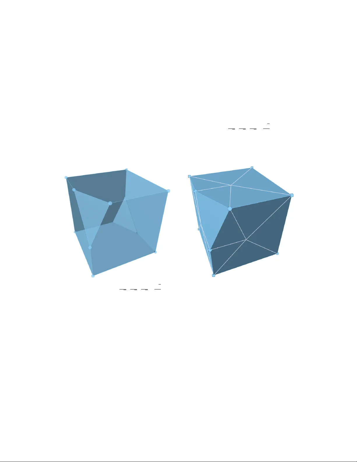
Critical moments of slices and slabs of the cube (and other pol yhedral norms) Marie-Charlotte Branden burg Jes ´ us A. De Lo era Y u Luo Chiara Meroni Abstract In this article, w e presen t a unified algebraic–com binatorial framew ork for computing explicit, piecewise rational, and com binatorially indexed parametric formulas for v olumes and higher momen ts of slices and slabs of p olyhedral norm balls. Our main metho d builds on prior work concerning a com binatorial decomp osition of the parameter space of all slices of a p olytope. W e extend this framew ork to slabs, and find a p olynomial-time algorithm in fixed dimension. W e also exhibit computational metho ds to obtain moments of arbitrary order for all slices or slabs of any polyhedral norm ball, and an algebraic framework for analyzing their critical p oints. In addition, we presen t an exp erimental study of the d -dimensional unit cub e. Our analysis reco vers and reinterprets the kno wn v olume formulas for slabs and slices of the tw o- and three- dimensional cubes, first obtained by K¨ onig and Koldobsky . Moreo ver, our method identifies a new complete family of fourteen rational functions giving the volumes of slices and slabs of the four-dimensional cub e. W e further compute explicit higher moments of slices and slabs in dimensions tw o and three, and derive explicit formulas for momen ts of arbitrary order for slices of the t w o-dimensional cub e, describing their critical points. 1 In tro duction Understanding the moments of con v ex b o dies, in particular high-dimensional p olyhedral norm balls, is a key to ol in conv ex geometry and analysis. In this pap er, moments are defined as in tegrals of p o w ers of co ordinates or norms (e.g., exp ectations lik e E [ | x i | k ] for a random p oint x in the norm ball). If K ⊂ R d is a cen trally symmetric con v ex b o dy and X is a measure uniformly distributed on K , then for every direction a in the unit sphere the one-dimensional marginal ⟨ a, X ⟩ has a densit y prop ortional to the volume of K in tersected with a h yp erplane orthogonal to a , which v aries with the distance of the hyperplane from the origin. More generally , the moments of slic es are exactly the momen t data of one-dimensional marginals. This p oint of view underlies muc h of asymptotic geometric analysis: information ab out the distribution of ⟨ a, X ⟩ as a v aries con trols the concen tration phenomena, the deviation inequalities, and the geometry of random sections and pro jections, themes that are at the heart of high-dimensional conv exity , and its functional-analytic consequences [ MS86 , Mil06 , Sc h14 ]. In short, the momen ts of conv ex b o dies are basic quantities that connect conv ex geometry , probabilit y , and the theory of Banach spaces. This pap er discusses ho w to efficiently compute the volumes and higher-order momen ts of slic es and slabs of p olyhe dr al norm b al ls , and shows how to reco v er explicit piecewise rational functions Keyw ords: slices of cub es, slabs of cub es, moment formulas, volume form ulas, critical p oin ts, polyhedral norm. MSC classes: 52A38, 52B55, 52-08 (primary); 68W30, 90C57 (secondary). 1 for them in terms of the slicing parameters, ( a, t ), a ∈ R d , where d is the ambien t dimension of the slab, and t ∈ R , t ≥ 0. Our metho ds are general and apply to an y scaled unit ball B d ∥·∥ := { x ∈ R d : ∥ x ∥ ≤ 1 2 } , of an arbitrary p olyhedral norm, such as the ℓ ∞ -ball that is the centered h yp ercub e B d ∞ = h − 1 2 , 1 2 i d . In what follows, let S d − 1 denote the unit sphere in R d , fix a = ( a 1 , . . . , a d ) ∈ S d − 1 and t ≥ 0, and write H ( a, t ) := { x ∈ R d : ⟨ a, x ⟩ = t 2 } , where ⟨· , ·⟩ is the standard scalar pro duct on R d . In other words, H ( a, t ) is a h yp erplane with unit normal vector a and Euclidean distance t/ 2 from the origin. This is the scaling of the slicing parameter that we use throughout the pap er. W e consider the slic e slice( a, t, ∥ · ∥ ) := B d ∥·∥ ∩ H ( a, t ) , and the slab slab( a, t, ∥ · ∥ ) := { x ∈ B d ∥·∥ : |⟨ a, x ⟩| ≤ t 2 } . F or M ∈ Z ≥ 0 w e fo cus on the M -th momen t Z slice( a,t, ∥·∥ ) d X i =1 x M i and Z slab( a,t, ∥·∥ ) d X i =1 x M i although, more generally , our metho d applies to all p olynomial integrands as giv en in [ BBDL + 11 ]. While we explain our metho ds for arbitrary p olyhedral norm balls, exp erimen tally we focus on the cub e B d ∞ . The geometry of hyperplane sections and slabs of the cub e b ecame an essential topic in conv ex geometry , combinatorics, and geometric functional analysis. A classical question is how large or small the ( d − 1)-dimensional volume of a hyperplane section can b e, and which choices of a and t mak e the slicing hyperplane extremal. F or minimal sections, V aaler pro ved that every k -dimensional central section of the cub e [ − 1 2 , 1 2 ] d has volume at least 2 k , with equality precisely for co ordinate-parallel sections [ V aa79 ]; this completed earlier w ork of Hadwiger [ Had72 ] and Hensley [ Hen79 ]. This also has extensions to ℓ p -balls via work of Meyer and Pa jor [ MP88 ]. F or maximal cen tral hyperplane sections, Ball sho wed that for the cub e [ − 1 2 , 1 2 ] d ev ery central h yp erplane section has ( d − 1)-dimensional v olume at most √ 2, with equalit y for normals prop ortional to e i ± e j [ Bal86 ]. Koldobsky’s F ourier-analytic framework gives general formulas for section volumes and connects these extremal questions to harmonic analysis [ Kol05 ]. In the setting of noncentral slicing, Barthe and Koldobsky related extremal slabs to Laplace-transform techniques [ BK03 ]; K¨ onig and Koldobsky studied ho w the volume of a slice or slab dep ends on the direction a and the offset parameter t , and obtained explicit formulas in dimensions d = 2 , 3 [ KK11 ]. Recen tly , P ournin and collab orators inv estigated shallow sections at a prescrib ed distance from the cen ter. They prov ed lo cal optimalit y results for diagonal directions in high dimension, for a range of offsets [ Pou23 ], see also [ DHUP21 , Sch14 ]. Momen ts of slices can b e viewed as integrals of monomials ov er ( d − 1)-dimensional sections of a con v ex b o dy , and thus capture how mass, curv ature, and directional structure are distributed along hyperplane cuts. Such momen ts naturally arise in geometric tomography [ Gar06 ] and Radon- t yp e reconstruction problems [ Nat01 ], where line or h yp erplane integrals enco de information used 2 in medical imaging, in v erse problems, computer vision, and shap e analysis, where momen t profiles along slices are used to reco ver or classify geometric ob jects [ FS94 ]. Motiv ated b y these applications, w e compute momen t formulas for slices and slabs of the cub e and analyze them in detail for slices in dimension 2. This w ork is complementary in b oth metho d and emphasis to prior work. Rather than start- ing from F ourier transforms or analytic inequalities, w e develop a unified algebr aic–c ombinatorial framew ork that partitions the parameter space into finitely many maximal c ham b ers in which the com binatorics is constan t, and computes volumes and momen ts on each c ham b er by abstract trian- gulations and the use of simplex-integration formulas from [ BBDL + 11 ]. This framework w as first in tro duced in [ BLM25 ] in the realm of slices of p olytop es; in this article, we extend this framew ork to slabs of cen trally symmetric p olytop es, i.e., p olyhedral norm balls, and illustrate the metho ds on the slices and slabs of the h yp ercub e, extending the results of [ KK11 ], and proving p olynomial algorithms in computing volume and momen t formulas for slices and slabs of polyhedral norm balls. 1.1 Our Con tributions Our first contribution is an explicit computational algorithm to obtain form ulas for momen ts of all slices and slabs of any p olyhedral norm ball. They turn out to b e piecewise rational and are v alid within a cham b er decomp osition of the unit sphere whic h parametrizes and gov erns volumes and higher momen ts. Algorithm for moments of slices and slabs of p olyhedral norm balls. Giv en a d -dimensional p olyhedral norm ball, our algorithm outputs piecewise rational form ulas for the moments of slices and slabs in p olynomial time in the input size. Note v olume is computed b y setting M = 0. Eac h piece of the function is supp orted on one cham b er of a hyperplane arrangement (partially restricted to the sphere). Combining this parametrization with an in tegration formula from [ BBDL + 11 ] yields the follo wing. Theorem 1 (P olynomial-time moment computation) . Fix d ∈ N and a p olyhe dr al norm ∥ · ∥ on R d . F or any M ∈ Z ≥ 0 , the algebr aic metho d intr o duc e d in Se ction 2 c omputes the M -th moments R slice( a,t, ∥·∥ ) P d i =1 x M i and R slab( a,t, ∥·∥ ) P d i =1 x M i in p olynomial time in the input size, as functions of ( a, t ) ∈ S d − 1 × R . The complete family of volume form ulas of slices and slabs of the 4 -cub e. The main computational contribution of this article concerns volumes and moments of the hypercub e up to dimension 4. Our computations recov er the known volume form ulas of K¨ onig and Koldobsky in dimensions 2 and 3 [ KK11 ]. W e extend their w ork b y finding explicit formulas for b oth slabs and slices in dimension 4, and their volumes are captured b y 14 distinct rational functions (up to the symmetry of the cub e). Theorem 2 (V olume form ulas of the 4-dimensional cub e) . L et a = ( a 1 , a 2 , a 3 , a 4 ) ∈ S 3 such that a 1 ≥ a 2 ≥ a 3 ≥ a 4 ≥ 0 , and let t ≥ 0 . The volumes of slic es and slabs of the 4 -dimensional cub e ar e pie c ewise r ational functions of ( a, t ) . Mo dulo signe d p ermutations of the c o or dinates, they admit a r epr esentation with exactly fourteen distinct r ational functions, e ach r epr esenting the volume of the c orr esp onding slic es or slabs for which ( a, t ) is c ontaine d in a maximal (close d) chamb er of a hyp erplane arr angement asso ciate d to B 4 ∞ . 3 Higher momen ts and critical-p oin t computations in low dimensions. W e complemen t the computational results with explicit piecewise rational functions for momen ts of order M = 1 , 2 , 3 , 4 for slices and slabs of the cube in dimensions 2 , 3 , 4, and demonstrate how to extract critical p oints b y algebraic metho ds. Moreo ver, for dimension 2 we prov e explicit closed formulas for R slice( a,t, ∥·∥ ∞ ) P d i =1 x M i for arbitrary M , as w ell as for their critical p oin ts. F or this purp ose, let us in tro duce cham b ers C 1 , 1 = { ( a, t ) ∈ S 1 × R | 0 < a 2 < a 1 , 0 < t < a 1 − a 2 } , C 1 , 2 = { ( a, t ) ∈ S 1 × R | 0 < a 2 < a 1 , a 1 − a 2 < t < a 1 + a 2 } . (1) F or details on the construction of these cham b ers, we refer the reader to Section 2.1 . Theorem 3 (Algebraic critical points of moments of square slices) . The critic al p oints of the M -th moment of slic es of the squar e, for fixe d t ∈ [0 , √ 2] , ar e exactly the p oints satisfying one of the fol lowing c onditions: a 1 − a 2 = t, or a 1 + a 2 = t, or ( a 1 , a 2 ) = (1 , 0) , or  a 2 2 + M  A + ( a 2 , t ) − t  ( M + 2) a 2 2 − 1  A − ( a 2 , t ) = 0 , ( a, t ) ∈ C 1 , 1 , M o dd , 2 a M 1 a 2 2 + ( a 2 2 + M ) A + ( a 2 , t ) − t ( a 2 2 ( M + 2) − 1) A − ( a 2 , t ) = 0 , ( a, t ) ∈ C 1 , 1 , M even , a M 1 ( t − a 1 ) M p ( a 1 , t, M ) + − a M 2 ( t − a 2 ) M p ( a 2 , t, M ) + a M 1 a M 2 ( a 3 1 − a 3 2 ) = 0 , ( a, t ) ∈ C 1 , 2 , wher e A + ( α, t ) = ( t − α ) M + ( t + α ) M , A − ( α, t ) = ( t − α ) M − ( t + α ) M α , p ( α, t, M ) = α 3 − t ( M + 2) α 2 + M α + t. Although we are not able to provide closed formulas for arbitrary momen ts of slices or slabs of h yp ercub es of an y higher dimension, we sho w that they share notable prop erties with the rational functions of the resp ective v olumes. Here, by degree of a rational function we mean the difference of degrees of numerator and denominator. Theorem 4 (Moments of slices and slabs) . F or any d ∈ N and M ∈ Z ≥ 0 , the moments R slice( a,t, ∥·∥ ∞ ) P d i =1 x M i and R slab( a,t, ∥·∥ ∞ ) P d i =1 x M i of slic es and slabs of the cub e B d ∞ ar e pie c ewise r ational functions whose pie c es ar e supp orte d on the same domains as the r ational function expr essions of the r esp e ctive vol- ume formulas of slice( a, t, ∥ · ∥ ∞ ) and slab( a, t, ∥ · ∥ ∞ ) . Mor e over, in al l c ompute d c ases M = 1 , 2 , 3 , 4 , the de gr e es of the r ational functions for the M − th moment c oincide with the de gr e es of the c orr e- sp onding volume formulas. F or the domains on which eac h rational expression is v alid, see T able 6 . This result is far from a coincidence but reflects a deep er structural fact: all moments of both slices and slabs are gov erned b y the same hyperplane arrangement, and it is precisely this shared com binatorial geometry that underlies our algebraic framework. Throughout this pap er, w e assume the reader is familiar with basic bac kground on p olytop es and hyperplanes. If needed, w e refer the reader to [ Gr ¨ u03 ]. Organization. Section 2 presen ts the algebraic-combinatorial framework that guides the con- struction and computation of the rational expressions for v olumes and momen ts of slices and slabs of a p olyhedral norm ball. In Section 3 w e present explicit formulas for the volumes and moments of slices and slabs of B d ∞ in d = 2 , 3 , 4 and of order M = 0 , 1 , 2 , 3 , 4. Moreo ver, in Section 3.1 we giv e closed-form formulas for all moments of slices of B 2 ∞ for arbitrary M ∈ Z ≥ 0 and their critical p oin ts. All explicit formulas discussed in the pap er are collected in the App endix . 4 2 Metho dology In this section, we lay out the theoretical framew ork underlying our computations. In Section 2.1 w e summarize the results of [ BLM25 ] for an algorithmic approach of computing volumes of slices of p olytop es. In Sections 2.2 to 2.4 we extend this framew ork to v olumes of slabs, then to higher momen ts of slices and slabs of cen trally symmetric p olytop es, i.e., p olyhedral norm balls. Finally , in Section 2.5 w e illustrate our algebraic approac h for the study of critical p oints of these functions. 2.1 Equiv alence Classes of Slices via V ertex Ordering W e b egin by introducing a construction that is cen tral to our metho d. Intuitiv ely , when sligh tly p erturbing a h yp erplane, the exp ectation is that its intersection with a fixed polytop e has the same com binatorial t yp e and that the t wo sections admit a common triangulation, therefore b earing the same volume and momen t formulas. W e use this observ ation to group h yp erplanes into equiv alence classes, where in eac h class the com binatorial t yp e for the asso ciated slices or slabs are the same. W e refine these equiv alence classes by chamb ers , whose definition is based on vertex orderings induced b y linear functionals asso ciated with the slicing hyperplanes. W e no w give a brief ov erview of this construction. F or more details, we refer to [ BLM25 , Sections 2.2 and 3.2]. Definition 2.1 (Sw eep arrangement) . L et P ⊂ R d b e a ful l-dimensional p olytop e with vertex set V ⊂ R d . The sweep arrangemen t asso ciate d to P is R ( P ) = { ( v − w ) ⊥ | v  = w ∈ V } , wher e v ⊥ = { x ∈ R d | ⟨ x, v ⟩ = 0 } is the hyp erplane ortho gonal to v . We denote by R i the r e gions of R ( P ) r estricte d to the unit spher e, namely the c onne cte d c omp onents of S d − 1 \ R ( P ) . Giv en a generic vector a ∈ S d − 1 ⊂ R d , the induc e d or dering on V is the unique lab eling V = { v 1 , . . . , v n } such that ⟨ a, v i ⟩ < ⟨ a, v i +1 ⟩ for all i = 1 , . . . , n − 1. The region R i of the sweep arrangemen t is by construction such that for all a ∈ R i , the linear functional ⟨ a, ·⟩ induces the same ordering v 1 , . . . , v n of the vertices of P . Definition 2.2 (Maximal Cham b er, [ BLM25 ]) . Consider a ful l-dimensional p olytop e P ⊂ R d with vertex set V = { v 1 , . . . , v n } , wher e the vertic es v i fol low the same or dering as describ e d ab ove. F or a fixe d r e gion R i of S d − 1 \ R ( P ) and a ve ctor a ∈ R i , any index j ∈ ⌊ n 2 ⌋ defines an op en interval I i,j ( a ) = { t ∈ R | 0 ≤ ⟨ a, v j ⟩ < t 2 < ⟨ a, v j +1 ⟩} for j > 0 , with I i, 0 ( a ) = { t ∈ R | 0 < t 2 < ⟨ a, v 1 ⟩} wher e v 1 is the first vertex of P such that ⟨ a, v 1 ⟩ > 0 . A maximal op en slicing cham b er , or just maximal c hamber , is the p olyhe dr on C i,j = { ( a, t ) ∈ S d − 1 × R | a ∈ R i , t ∈ I i,j ( a ) } ⊂ R d +1 . Regions control v e rtex orderings in direction space; c hambers refine this b y tracking which faces of P are intersected as t v aries. W e say that t w o p olytop es Q 1 , Q 2 from the same cham b er admit the same triangulation if there exist triangulations T i of Q i and a bijection b etw een the sets of all v ertices in T 1 and those in T 2 , which sends simplices to simplices. W e collect in the following lemma a few useful prop erties of the maximal cham b ers. Lemma 5 ([ BLM25 , Subsections 2.2 and 3.2]) . A maximal chamb er satisfies the fol lowing pr op er- ties: (i) F or al l ( a, t ) ∈ C i,j , the hyp erplane H ( a, t ) = { x ∈ R d | ⟨ a, x ⟩ = t 2 } interse cts the same fixe d set of e dges of P . 5 (ii) Conse quently, for any ( a 1 , t 1 ) , ( a 2 , t 2 ) ∈ C i,j , the slic es P ∩ H ( a 1 , t 1 ) and P ∩ H ( a 2 , t 2 ) ar e c ombinatorial ly e quivalent, thus admit the same triangulation. (iii) Each c o or dinate of a vertex of P ∩ H ( a, t ) is a r ational function in the variables ( a, t ) . This r ational function is valid for al l ( a, t ) ∈ C i,j . (iv) Conse quently, the volume of P ∩ H ( a, t ) and the moment R P ∩ H ( a,t ) P d i =1 x M i ar e r ational func- tions in the variables ( a, t ) , when r estricte d to ( a, t ) ∈ C i,j . As stated in Theorem 1 of [ BLM25 ], given any p olytop e P ⊂ R d , there are only finitely many slicing cham b ers of P . Theorem 5 implies that the volume formulas and momen t formulas for a family of slices restricted to a c ham b er C i,j is determined by the fixed set of edges that the corre- sp onding hyperplanes in tersect. In order to obtain this set, it suffices to find a single representativ e ( a rep , t rep ) ∈ C i,j . Given a rep , a canonical c hoice is t rep = 1 2 ( ⟨ a rep , v j ⟩ + ⟨ a rep , v j +1 ⟩ ). This is enough to compute the intersecting set of edges, the combinatorial t yp e of the slices, the parametrization of the vertices, and finally the volume and momen t formulas in the maximal cham b er C i,j . See [ Sch86 ] for details. Supp ose we kno w that H ( a, t ), where ( a, t ) ∈ C i,j , in tersects an edge e of p olytop e P . Let v and w b e the tw o vertices of e . The parametrization of the v ertices of a slice w orks as follows. The in tersection p oint x a ( t ) = e ∩ H ( a, t ) is a v ertex of the slice P ∩ H ( a, t ). Its co ordinates are giv en b y x a ( t ) = t 2 ⟨ a, w − v ⟩ ( w − v ) + ⟨ a, w ⟩ v − ⟨ a, v ⟩ w ⟨ a, w − v ⟩ , (2) whic h is a rational function in the v ariables ( a 1 , . . . , a d , t ) ∈ S d − 1 × R . These observ ations imply a simple algorithm to obtain the piecewise rational v olume formula of P ∩ H ( a, t ) in terms of a and t : First, for eac h maximal slicing cham b er C i,j of the sw eep arrangement R ( P ), compute a single ( a rep , t rep ) ∈ C i,j . F rom P ∩ H ( a rep , t rep ) w e obtain the com binatorial type of all slices P ∩ H ( a, t ) for all ( a, t ) ∈ C i,j , with whic h we can compute a common triangulation for this family of slices. The set of edges of P which are in tersected by H ( a rep , t rep ) can b e used to compute the parametrization of the v ertices of P ∩ H ( a, t ) for all ( a, t ) ∈ C i,j . Using this information, one can compute the rational function expression for the volume of a simplex in the common triangulation. Summing the volume of the simplices, we obtain the v olume form ulas for the en tire family P ∩ H ( a, t ) , ( a, t ) ∈ C i,j . Iterating ov er all maximal slicing c ham b ers then yields the piecewise rational function. 2.2 F rom Slices to Slabs The metho d describ ed in Section 2.1 can no w b e generalized from ( d − 1)-dimensional slices of a p olytop e to its d -dimensional slabs. W e b egin by discussing in some detail what the v ertices of a slab are, and how to triangulate it in order to compute a volume expression of a slab within a single maximal slicing cham b er. V ertices of a slab A slab has tw o t yp es of v ertices. The first type consists of vertices of the p olyhedral norm ball P itself. These are easily iden tified b y collecting all v ertices v i of P suc h that |⟨ a, v i ⟩| ≤ t 2 . The second t yp e consists of v ertices created by the in tersection of the hyperplanes H ( a, t ) and H ( a, − t ) with edges of P . ( 2 ) ensures the second t yp e of vertices has a rational expression on parameters ( a, t ). T ogether w e hav e the set of v ertice s V , which are used directly in the v olume computation. 6 T riangulation computation In order to find the rational function expressions for the volume of slab( a, t, ∥ · ∥ ), w e triangulate it and find the volume of eac h simplex. The triangulation we use in this pap er is the b aryc entric triangulation . This is a classical and widely used metho d in computational and combinatorial geometry [ Ede87 , Zie95 , DLRS10 ]. In tuitiv ely , after determining the faces of the slab via their supp orting hyperplanes, each tw o-dimensional face is sub divided b y in tro ducing its barycen ter and coning to the edges. k -dimensional faces are triangulated inductiv ely b y coning to the barycen ters of all its k − 1-dimensional b ounding faces. This pro duces the canonical barycen tric sub division of the slab. W e then compute the volume of the slab by adding the (signed) determinan ts of simplices in the triangulation. This approach allo ws us to compute volume and momen ts symbolically as piecewise rational functions in ( a, t ). Example 1 . Consider the slab of the three-dimensional cub e slab(( 2 √ 6 , 1 √ 6 , 1 √ 6 ) , √ 6 2 , B 3 ∞ ), displa yed in Figure 1 , left, and on the righ t its barycentric triangulation. Eac h supp orting hyperplane of the cub e con tributes one facet of the slab, and coning from a single interior p oint of each facet induces a barycen tric triangulation. Figure 1: Left: slab(( 2 √ 6 , 1 √ 6 , 1 √ 6 ) , √ 6 2 , B 3 ∞ ). Right: its barycentric triangulation, from Example 1 . Lemma 6. L et P = B d ∥·∥ b e a p olyhe dr al norm b al l. Given two hyp erplanes H ( a, t ) and H ( a ′ , t ′ ) that b elong to the same maximal slicing chamb er, then the asso ciate d slabs slab( a, t, ∥ · ∥ ) and slab( a ′ , t ′ , ∥ · ∥ ) have the same c ombinatorial typ e and the same p ar ametrization of their vertic es. Mor e over, the volume of e ach p ar ametrize d slab is a r ational function. As a c onse quenc e, by listing al l p ossible maximal chamb ers, we r e c over the volume formulas of al l slabs of P . By c ontinuity of the volume function, the formulas asso ciate d with two adjac ent chamb ers agr e e along their c ommon b oundary. Ther efor e, if a slicing dir e ction lies on the b oundary b etwe en two maximal slicing chamb ers, its volume may b e c ompute d using the formula fr om either chamb er. Pr o of. As mentioned in Section 2.1 , the num b er of maximal slicing cham b ers is finite. Fix suc h a maximal cham b er C i,j ⊂ S d − 1 × R . By part (i) of Theorem 5 , the h yp erplane H ( a, t ) intersects the same set of edges of P for any c hoice of ( a, t ) ∈ C i,j . Central symmetry of P implies the same conclusion for H ( a, − t ). The parametrization ( 2 ) of a vertex obtained b y intersecting an e dge of P with either H ( a, t ) or H ( a, − t ) is a rational function in C i,j . Moreo v er, the set of v ertices of P 7 con tained in the strip { x ∈ R d | − t 2 < ⟨ a, x ⟩ < t 2 } b etw een the tw o hyperplanes is fixed, since all a ∈ R i determine the same v ertex ordering. Thus, the com binatorial type and the parametrization of the vertices of slab( a, t, ∥ · ∥ ) is fixed for all ( a, t ) ∈ C i,j , in particular for ( a ′ , t ′ ). Fix now a triangulation of the slabs from C i,j , such that the set of vertices forming a simplex dep ends only on the face lattice of the slabs of P in this cham b er (we sa w this is done with barycen tric triangulations). Similarly to the ab ov e, all vertices of the triangulation admit rational parameterizations. The volume of a slab can then b e computed as follows. F or each d -dimensional simplex with vertices s 0 , . . . , s d , up to sign the volume equals 1 d ! det( s 1 − s 0 , . . . , s d − s 0 ) . (3) As for slices, the simplices hav e co dimension one, and therefore if their vertices are denoted by s 1 , . . . , s d , their volume can b e computed as v ol(∆) = 1 ( d − 1)! det  s 2 − s 1 , s 3 − s 1 , . . . , s d − s 1 , a ∥ a ∥  , (4) where a is an y v ector orthogonal to the affine span of the simplex. Since the affine span is b y definition of the slice H ( a, t ) and a ∈ S d − 1 , the norm can b e dropp ed. In b oth cases, the volume of one simplex is a rational function on v ariables ( a, t ). Since each of these v ertices is a rational function in v ariables a 1 , . . . , a d , t , the same holds for the volume of the simplex. The volume of slab( a, t, ∥ · ∥ ) is then the sum of the volumes of these parametric simplices, and thus a rational function as well. W e note that this rational function expression is not only v alid on the open set C i,j , but, b y contin uit y of the volume function, also on the b oundary of its Euclidean closure. Theorem 6 implies that the num b er of rational function expressions for the volume of slabs is finite, and that the n um b er of such expressions is b ounded from ab o ve by the n umber of maximal slicing cham b ers C i,j . Moreo v er, the pro of of Theorem 6 rev eals that small mo difications of the algorithm describ ed in Section 2.1 yield an algorithm to compute rational function expressions for the v olume of slabs in terms of a and t . 2.3 V olume and Higher Momen t F ormulas T o compute the momen ts of slices and slabs, our approac h b egins b y triangulating them, as outlined in Section 2.2 . F or each simplex in the triangulation, we compute rational functions for the momen ts using [ BBDL + 11 , Lemma 8], which provides a closed-form expression for the integral of a p o w er of a linear form ov er a simplex. Let M ∈ Z ≥ 0 , and let ∆ = con v ( s 1 , s 2 , . . . , s n +1 ) b e an n -dimensional simplex in R d . F or an y linear form ℓ on R d , Z ∆ ℓ M d x = n ! v ol(∆) M ! ( M + n )! X k ∈ N n +1 | k | = M ⟨ ℓ, s 1 ⟩ k 1 · · · ⟨ ℓ, s n +1 ⟩ k n +1 , (5) where w e in tegrate with resp ect to the standard Lebesgue measure. In the case of M = 0, the in tegral in Equation ( 5 ) reduces to computing the v olume of a simplex. W e saw in the pro of of Theorem 6 that the volume of a full-dimensional simplex can b e expressed (up to sign) as a determinant (see Equations ( 3 ) and ( 4 )). Therefore, w e can use that form ula for the full-dimensional simplices in the triangulation of the slices and slabs. Recall from Equation ( 2 ) that every vertex (of slices and slabs) is a rational function of ( a, t ) ∈ C i,j for eac h c hamber. Thus, Equation ( 5 ) implies that for an y slice or slab all the M -momen ts are piecewise rational functions in ( a, t ) ∈ S d − 1 × R . 8 R emark 7 . W e stress that to mak e the moment form ulas of the slices piecewise rational, one needs to require a ∈ S d − 1 . Otherwise, for a ∈ R d , the form ulas are merely semialgebraic functions, as they hav e a dep endence on ∥ a ∥ . How ev er, in the case of slabs, since there is no normal vector a in v olv ed in the v olume expression of the simplex, one could allow a ∈ R d . In order to make the narration coheren t and the description of slices and slabs non-redundant, w e require a ∈ S d − 1 in b oth cases. W e conclude this section b y presen ting a concrete computational example of a moment calcula- tion of one sp ecific family of slabs of the 2-dimensional cub e. Example 2 . Assume d = 2 and M = 2. T o compute all rational functions for the second moment of the slabs of the square, we b egin by finding the maximal op en slicing cham b ers. Up to symmetry (p erm utations and reflections), there is exactly one p ossible vertex ordering, namely one region of the sw eeping arrangement whic h we denote R 1 = { ( a 1 , a 2 ) ∈ S 1 | a 1 > a 2 > 0 } . This induces the vertex ordering v 1 , v 4 , v 2 , v 3 , as shown in Figure 2 , center. Then, the ranges for t > 0 asso ciated with this region are I 1 , 1 ( a ) = (0 , 2 ⟨ v 2 , a ⟩ ) , I 1 , 2 ( a ) = (2 ⟨ v 2 , a ⟩ , 2 √ 2) . Indeed, when t/ 2 ∈ I 1 , 1 ( a ), the slab is a parallelogram (sho wn in Figure 2 , left) and when t ∈ I 1 , 2 ( a ), the slab is a hexagon (shown in Figure 2 , righ t). Th us, to find form ulas for all combinatorially differen t slabs in this region, we need to in vestigate the tw o asso ciated slicing cham b ers C 1 , 1 and C 1 , 2 , in tro duced already in ( 1 ). Let a rep = 1 √ 5 (2 , 1) ∈ R 1 b e a represen tativ e v ector, then I 1 , 1 ( a rep ) = (0 , 1 √ 5 ) and I 1 , 2 ( a rep ) = ( 1 √ 5 , 3 √ 5 ). After choosing tw o representativ es t rep for t , namely 1 2 √ 5 ∈ I 1 , 1 ( a rep ) and 2 √ 5 ∈ I 1 , 2 ( a rep ), w e can find the edges that are intersected b y H ( a rep , t rep ), and with this the parametric expressions for the vertices of the tw o types of slabs. Since the pro cedure is analogous in b oth c hambers, we only illustrate the hexagonal case where ( a rep , t rep ) ∈ C 1 , 2 . a rep = 1 √ 5 (2 , 1) v 4 v 3 v 2 v 1 Figure 2: Cen ter: hyperplane sweep across B ∥·∥ ∞ in R 2 . Left: quadrilateral slab asso- ciated to ( a rep , t rep ) ∈ C 1 , 1 . Right: hexagonal slab asso ciated to ( a rep , t rep ) ∈ C 1 , 2 . The rational functions describing the volumes of these t wo types of slabs are distinct and are computed in Example 2 . When t ∈ I 1 , 2 ( a rep ), the slab has six vertices. F our of them arise from the in tersection of the square with the sweeping h yp erplanes at distance t 2 from the origin: these are ( 1 2 , t − a 1 2 a 2 ) , ( t − a 2 2 a 1 , 1 2 ) , ( − 1 2 , a 1 − t 2 a 2 ) , and ( a 2 − t 2 a 1 , − 1 2 ). Additionally , there are tw o vertices of the slab whic h are v ertices of the square itself. T o find these, w e chec k the inequalities |⟨ a rep , v i ⟩| ≤ t/ 2 at all vertices v i of the square. Thus, the complete list of v ertices of the hexagonal slab is n ( − 1 2 , 1 2 ) , ( 1 2 , − 1 2 ) , ( 1 2 , t − a 1 2 a 2 ) , ( t − a 2 2 a 1 , 1 2 ) , ( − 1 2 , a 1 − t 2 a 2 ) , ( a 2 − t 2 a 1 , − 1 2 ) o . Next, we triangulate the slab by first identifying all its edges. T able 1 shows the defining equations 9 (left column) of all six edges, and their v ertices (right column) as a function of ( a, t ) ∈ C 1 , 2 . T o eac h pair of vertices of a fixed edge, we add the barycenter of the slab, namely the origin (0 , 0), to obtain a triangulation of the slab in to six t wo-dimensional simplices. Finally , we use Equations ( 3 ) and ( 5 ) to compute the second moment of eac h simplex and add them up to get the final rational function: Z slab( a,t, ∥·∥ ) x 2 1 + x 2 2 = a 1 − a 2 + t 32 a 1 − a 1 − a 2 − t 32 a 2 + ( a 2 1 + a 1 a 2 + a 2 2 − a 1 t − 2 a 2 t + t 2 )( a 1 − a 2 + t ) 96 a 3 1 − ( a 2 1 + a 1 a 2 + a 2 2 − 2 a 1 t − a 2 t + t 2 )( a 1 − a 2 − t ) 96 a 3 2 + ( a 2 1 − a 1 a 2 + a 2 2 − 2 a 1 t + a 2 t + t 2 )( a 1 + a 2 − t ) t 96 a 1 a 3 2 + ( a 2 1 − a 1 a 2 + a 2 2 + a 1 t − 2 a 2 t + t 2 )( a 1 + a 2 − t ) t 96 a 3 1 a 2 , for all ( a, t ) in the top ological closure of C 1 , 2 . 2.4 Pro of of Theorem 1 Pr o of. First, w e b ound the num b er of maximal cham b ers asso ciated to B ∥·∥ . By [ BLM25 , Proposi- tion 3.9], at a fixed dimension d , the num b er of maximal c hambers is p olynomial in the num b er of v ertices n of the norm ball ( O ( n 2 d +1 2 d )). Next, w e show the time needed to compute one slab/slice in one cham b er is p olynomial in the input size. Let B ∥·∥ b e the unit ball of the p olyhedral norm ∥ · ∥ and assume that it has n v ertices. Theorem 6 com bined with Equation ( 5 ) prov es that on each of the maximal cham b ers C i,j , the moments of the slices and slabs of B ∥·∥ are parametric rational functions. It remains to show that our metho d runs in p olynomial time in the input size, whic h is the n um b er of bits needed to write do wn the p olytop e ( n is b ounded by the bit-size of the p olytop e, see [ Sch86 ]), which is the slice or slab in consideration. Consider slice( a, t, ∥ · ∥ ) as a ( d − 1)-dimensional polytop e and slab( a, t, ∥ · ∥ ) as a d -dimensional p olytop e. Since the arguments are identical in b oth cases, it suffices to establish the claim for one of them; the other follows. Thus, from now on, we fo cus on the p olytop e S = slab( a, t, ∥ · ∥ ). Let n denote the num b er of vertices of S . Each d -dimensional simplex in the barycentric triangulation of S has d + 1 vertices. Our goal is to b ound the num b er of simplices in the triangulation of S using the Upp er Bound Theorem. By definition of the barycentric triangulation, for any simplex ∇ = conv { v 1 , v 2 , . . . , v d +1 } ⊂ S , there exists a chain (b y inclusion) of faces F i of dimension i of S , namely , F 2 ⊂ F 3 ⊂ · · · ⊂ F d = S, suc h that v 1 , v 2 ∈ F 2 , v 3 ∈ F 3 , . . . , v d +1 ∈ F d and the v i are the barycenters of F i for all i > 2. W e can therefore upp er-b ound the num b er of simplices using the pro duct of the maximal n um b er equation edge v ertices x 1 = 1 / 2 { ( 1 2 , − 1 2 ) , ( 1 2 , t − a 1 2 a 2 ) } x 1 = − 1 / 2 { ( − 1 2 , 1 2 ) , ( − 1 2 , a 1 − t 2 a 2 ) } x 2 = 1 / 2 { ( − 1 2 , 1 2 ) , ( t − a 2 2 a 1 , 1 2 ) } x 2 = − 1 / 2 { ( 1 2 , − 1 2 ) , ( a 2 − t 2 a 1 , − 1 2 ) } ⟨ a, x ⟩ = t/ 2 { ( 1 2 , t − a 1 2 a 2 ) , ( t − a 2 2 a 1 , 1 2 ) } ⟨ a, x ⟩ = − t/ 2 { ( − 1 2 , a 1 − t 2 a 2 ) , ( a 2 − t 2 a 1 , − 1 2 ) } T able 1: F acet-defining equalities of slab( a rep , t rep , ∥ · ∥ ∞ ) and corresp onding vertices, from Example 2 . 10 of faces of each dimension i = 1 , . . . , d . By the Upp er Bound Theorem [ McM70 ], any d -dimensional p olytop e with n vertices has at most as many i -dimensional faces as the cyclic p olytop e ∆( n, d ). F or 1 ≤ i ≤ d − 1, the face num b ers f i of the cyclic p olytop e satisfy f i (∆( n, d )) = n − ( d − 2 ⌊ d 2 ⌋ )( n − i − 2) n − i − 1 n X j =0  n − 1 − j i + 1 − j  n − i − 1 2 j − i − 1 + d − 2 ⌊ d 2 ⌋  , see [ Gr ¨ u03 , Chapter 9.6]. F or fixed d and i , this is a p olynomial in n . Consequen tly , the num b er of simplices pro duced from the barycentric triangulation pro cedure is b ounded from ab o ve by the pro duct of the num b er of faces of the cyclic p olytop e: d − 1 Y i =1 f i (∆( n, d )) . Note that, fixing d , this b ound is p olynomial in n , and thus it is b ounded by the input size of p olyhedral norm ball B ∥·∥ . Since the momen t of an individual simplex can b e computed in p olynomial time in their input bit-size [ BBDL + 11 ], this b ound implies that the total running time for computing any moment of one slice( a, t, ∥ · ∥ ) or slab( a, t, ∥ · ∥ ) is p olynomial in the input size. Hence, momen t computation for all slices and slabs of a given polyhedral norm is p olynomial-time in the bit-size of the input. 2.5 Algebraic analysis to reco ver critical p oints of momen ts Giv en the structure of the maximal op en slicing cham b ers, the output of our algorithm for p olyhedral norm balls consists of a list of rational functions, eac h asso ciated to a maximal cham b er C i,j , i = 1 , . . . , m and j = 1 , . . . , n − 1. W e are interested in computing the maxima and minima (or, more generally , the critical p oin ts) of the piecewise rational function f , which is rational in each C i,j . There are tw o cases for a critical p oin t ( a, t ) of f : 1. ( a, t ) ∈ C i,j is a critical p oint of the rational function defining f in this op en cham b er; 2. ( a, t ) ∈ ∂ ( C i,j ). F or the second type of critical p oints, w e need to analyze the v alue of each rational function along the b oundary of its cham b er. How ever, for the first type of critical p oints, we can also p erform a qualitativ e algebraic analysis. This is the fo cus of the current section. F or more bac kground on computation with algebraic ideals and v arieties, we refer to [ CLO15 ]. W e are in terested in the critical p oin ts at fixed v alues of t , and therefore w e only consider deriv atives with resp ect to the v ariable a . F or a rational function p on the sphere, the critical p oints are the zeros of its spherical gradient, namely ∇ S d − 1 p ( a ) = ∇ R d p ( a ) − ⟨∇ R d p ( a ) , a ⟩ a, where ∇ R d denotes the standard gradient in R d . This expression is a vector of rational functions. Ho w ev er, since we are interested in the zeros of the gradient, we can study , without loss of gen- eralit y , the common zeros of the numerators of the gradient entries. Indeed, by construction, the denominators do not v anish in the in terior of a c hamber, so the zeros of the gradient coincide with the zeros of these numerators. This information can b e pac k aged in an ideal of p olynomials. In particular, since we are only in terested in the underlying set of (real) critical p oints, and not in m ultiplicities or scheme-theoretic 11 structure, it is enough to pass to the radical of the ideal, which b y definition collects all p olynomials v anishing at the prescrib ed p oints. Therefore, for each maximal cham b er C i,j , the radical ideal in the v ariables ( a, t ) ∈ S d − 1 × R necessary for the critical p oints is the radical of the ideal generated b y the numerators of the expressions appearing in ∇ S d − 1 f | C i,j . The dimension and degree of I i,j pro vide information ab out the critical p oin ts: in the case of dimension 0, the degree of the ideal equals the num b er of critical p oints ov er the complex n umbers, and therefore giv es an upp er b ound on the num b er of real critical p oints. F or higher-dimensional ideals, one can instead study the structure of the corresp onding solution sets. Finally , we can de c omp ose I i,j in order to divide the critical points into families sharing similar algebraic prop erties, for instance p oin ts satisfying the same minimal p olynomial relations. This analysis can be p erformed ov er Q in sev eral computer algebra soft w ares, primarily Macaulay2 [ GS ] or Oscar.jl [ OSC25 , DEF + 25 ]. In the remainder of this subsection, we present an exhaustive example in which we exploit these tec hniques. This computation is feasible in dimensions 2, 3, and partially in dimension 4, see Theorem 8 . Figure 3: Left: The t w o fundamental open slicing c ham b ers of the tw o-dimensional cub e, displa y ed in co ordinates ( α, t ), where ( a 1 , a 2 ) = (cos α, sin α ). Righ t: The piecewise rational function f = { f (2 , 2) 1 , f (2 , 2) 2 } of the second moment from Example 3 , together with its maxima (black curv e) for each v alue of t . Example 3 . W e contin ue Example 2 for the square and the second momen ts of its slabs. There are t w o maximal op en slicing cham b ers ( 1 ), denoted by C 1 , 1 (Figure 3 , left, green) and C 1 , 2 (Figure 3 , left, red). Hence, there are tw o relev ant rational functions whic h, for a ∈ S 1 , read g (2 , 2) 1 = t 3 + t 12 a 3 1 , g (2 , 2) 2 = − t 4 +4( a 3 1 + a 3 2 ) t 3 +(12 a 2 1 a 2 2 − 6) t 2 +4  a 5 1 + a 5 2 + a 2 1 a 2 2 ( a 1 + a 2 )  t +(8 a 3 1 a 3 2 − 1) 96 a 3 1 a 3 2 , resp ectiv ely , where w e use the notation of Section A.4.2 . The asso ciated radical ideals are I 1 , 1 =  a 2 1 + a 2 2 − 1 , a 2 ( t 3 + t )  , I 1 , 2 =  a 2 1 + a 2 2 − 1 , (2 a 2 2 − 1)( t 4 + 1) + 4  a 1 ( a 2 2 − 1) 2 − a 5 2  ( t 3 + t ) + 2(2 a 2 2 − 1)(2 a 4 2 − 2 a 2 2 + 3) t 2  . Both ideals hav e co dimension 2 in the three-dimensional space C 2 × C , and we interpret them as one-parameter families of critical p oints, where t pla ys the role of the parameter. The ideal I 1 , 1 has degree 8 and decomp oses into four prime ideals:  a 2 , a 1 − 1  ,  a 2 , a 1 + 1  ,  a 2 1 + a 2 2 − 1 , t  ,  a 2 1 + a 2 2 − 1 , t 2 + 1  . The first t w o ideals describ e t wo families of critical points parametrized b y ( ± 1 , 0 , t ). The third ideal corresp onds to the sphere S 1 × { 0 } , and the fourth one to the spheres S 1 × {± i } , where i = √ − 1. 12 Notice that none of these p oints b elong to the op en slicing c hamber C 1 , 1 . Therefore, the interior of this c hamber do es not contribute an y critical p oint. Rep eating the same pro cedure for the ideal I 1 , 2 , we find that its degree is 16 and that it decomp oses as  a 2 1 + a 2 2 − 1 , a 1 − a 2  ,  a 2 1 + a 2 2 − 1 , t − a 1 − a 2  ,  a 2 1 + a 2 2 − 1 , t ( a 1 + a 2 ) − 1  ,  a 2 1 + a 2 2 − 1 , t 2 − 2 t ( a 3 2 − a 1 a 2 2 + a 1 ) + 1  . These ideals describ e, resp ectively , families of critical p oints of the form ( ± ( 1 √ 2 , 1 √ 2 ) , t ), ( a 1 , a 2 , a 1 + a 2 ), ( a 1 , a 2 , 1 a 1 + a 2 ), and ( a 1 , a 2 , ϕ ± ( a )), where ϕ ± ( a ) = a 3 2 − a 1 a 2 2 + a 1 ± q  − a 1 a 2 2 + a 1 + a 3 2  2 − 1 . The first tw o families lie on the b oundary of C 1 , 2 and therefore do not contribute critical points in the in terior of the cham b er. The third family , on the other hand, lies in C 1 , 2 for all a ∈ R 1 (as in Definition 2.2 ), hence for t ∈ ( 1 √ 2 , 1). This family is sho wn in Figure 4 , cen ter, for t = 0 . 8. The en tire curv e of critical p oin ts in the interior of the slicing cham b er corresp onds to the black curve in Figure 3 , right, lying inside the red surface. Finally , the last family of points is never real in C 1 , 2 . Figure 4: The function f ( α, t rep ) = { f (2 , 2) 1 ( α, t rep ) , f (2 , 2) 2 ( α, t rep ) } of the second momen t of the tw o-dimensional cub e from Example 3 , where ( a 1 , a 2 ) = (cos α , sin α ) and t rep = 0 . 2 , 0 . 8 , 1 . 2 from left to right. The green part of each curve is its restriction to C 1 , 1 , and the red part is its restriction to C 1 , 2 . Only in the central figure is there a maximum in the in terior of a slicing cham b er. One can repeat analogous computations for all the rational functions produced b y our algorithm. T able 2 summarizes these computations for the rational functions describing the v olume of slices of the three-dimensional cub e B 3 ∞ , which are listed explicitly in Section A.2.1 . The table was obtained using Macaulay2 . F or each rational function, w e compute the dimension and degree of the asso ciated radical ideal, as well as its decomposition into irreducible comp onen ts. This decomp osition rev eals ho w many irreducible components the ideal has, corresp onding to distinct families of critical p oints. F or eac h such comp onent, we also record its dimension and degree. Note that when comp onents of differen t dimensions are presen t, the rep orted degree of the ideal refers to the degree of the top-dimensional comp onent. Analogous computations can be carried out for the remaining rational functions listed in the App endix. R emark 8 . F or larger ideals (in terms of the n um b er of v ariables or the degrees of the generators), some Macaulay2 computations may fail to terminate. In such cases, one can instead exploit the 13 V olume formulas dim I deg I dim of irr. comp onents deg of irr. comp onents f 1 1 2 (1,1) (1,1) f 2 1 8 (1,1,1) (2,2,4) f 3 2 2 (2,1,1,1,1) (2,2,4,4,4) f 4 1 24 (1,1,1,1,1) (2,4,6,6,6) f 5 1 20 (1,1,1,1) (2,2,8,8) T able 2: I is the ideal of the critical p oints of the corresp onding volume formula for the slices of B 3 ∞ . The irreducible comp onents are o ver Q . The functions f i are giv en in Section A.2.1 . numeric al irr e ducible de c omp osition implemen ted in HomotopyContinuation.jl [ BT18 ] to obtain information ab out the irreducible comp onents of the ideals ov er R . This decomp osition may differ from the one o v er Q . Indeed, the ideal generated b y the univ ariate p olynomial x 2 − 2 is irreducible o v er the field of rational num b ers, but it decomposes o ver the reals into the t w o prime ideals ( x − √ 2) and ( x + √ 2). F or this reason, if the decomp osition w ere p erformed ov er R , the last tw o columns corresp onding to f 2 , f 3 , and f 4 in T able 2 would c hange. In particular, their irreducible one- dimensional components ov er R w ould be more n umerous and hav e degrees (1 , 1 , 2 , 4), (1 , 1 , 4 , 4 , 4), and (1 , 1 , 2 , 2 , 6 , 6 , 6), resp ectively . W e lea ve as a p ossible direction for future research the problem of determining which of these comp onen ts actually con tribute to real critical p oin ts of the volume or moment functions in each c ham b er. 3 Slices and Slabs of Lo w-Dimensional Cub es In this section, w e present computational exp eriments inv estigating rational-function expressions for the volumes and moments of slices and slabs of the infinity norm ball, the d -dimensional cub e B d ∞ for d = 2 , 3 , 4 and momen ts M = 0 , 1 , 2 , 3 , 4. Moreo ver, in the case of slices of the 2-dimensional cub e, we giv e a complete theoretical description of all moments of slices, as w ell as their critical p oin ts, for all M ∈ Z ≥ 0 . All computations were carried out sym b olically in SageMath [ Sag24 ], follo wing the metho d in tro duced in Section 2 . All rational functions are prin ted in the App endix . The code and rational functions in digital form are publicly a v ailable at https://github.com/Rai nCamel/slab_of_the_poly_norms Fixing a region R i ⊂ S d − 1 and a represen tativ e direction a rep ∈ R i , one obtains 2 d − 1 distinct t -ranges I i,j ( a rep ). Let t rep b e the midp oint of such an interv al, as describ ed in Section 2.1 . Since slices and slabs share the same maximal cham b er C i,j , eac h suc h case giv es rise to one corresponding v olume form ula and a family of momen t formulas, indexed b y M . Due to the symmetry of the infinity norm ball, it suffices to compute all cham b ers containing p oin ts a ∈ S d − 1 satisfying a 1 ≥ a 2 ≥ · · · ≥ a d ≥ 0. But even after this restriction, we will see that some rational function expressions are defined on m ultiple cham b ers. F or example, the expressions f 5 and g 5 (see the next paragraph for their definitions) in T able 5 app ear in some in terv al of all six regions R i . This happ ens b ecause in all those cham b ers C i,j , the hyperplane H ( a, t ) separates one v ertex of the cube from all the others, resulting in an equiv alent family of slices or slabs. Other rep etitions arise in a similar manner. R emark 9 . W e note that in highly symmetric situations, such as the unit cube, there is rep etition of the rational function expressions on different c hambers, up to p ermutation or reflection of v ariables. Ultimately it is the com binatorial t yp e that controls the v olume/moment formulas, but enumerating 14 through all maximal cham b ers gives a systematic wa y to find all p ossible combinatorial types of slices or slabs of a given polyhedral norm ball. Notation. F or notation, w e use f ( M ,d ) k to denote the k -th rational expression of the M -th momen t of the slice of the d -dimensional cub e B d ∞ , and use g ( M ,d ) k to denote the k -th rational expression of the M -th momen t of the slab of the d -dimensional cub e B d ∞ . W arning. In this section, we sometimes omit the sup erscripts ( M , d ) from the formulas listed in the tables when the con text is clear, i.e. w e use f k , g k instead of f ( M , 2) k , g ( M , 2) k . When am biguit y arises, please refer to the table captions or closest explanation of dimension and moment. 3.1 B 2 ∞ W e giv e explicit form ulas for volumes, as w ell as higher momen ts of slices and slabs of B 2 ∞ for momen t M = 1 , 2 , 3 , 4. They app ear in Sections A.1 and A.4 and were computed with the metho d explained in Section 2 . Restricted to a 1 ≥ a 2 ≥ 0, T able 3 follows K¨ onig and Koldobsky [ KK11 ], and identifies the largest range of t as a function of a in whic h a certain rational function is v alid (see T able 3 ). This table further indicates for each case whic h of the v olume form ulas giv en in Section A.1 are v alid. The given volume form ulas in dimension 2 agree with the ones given in [ KK11 ], we presen t them here for completeness. W e extend their results b y pro viding similar formulas for higher moments ( M = 1 , 2 , 3 , 4) in Section A.4 . By construction, the form ulas for higher moments are defined on the same regions as the v olumes. T able 3 is therefore also a v alid table for the moment formulas in Section A.4 . t-range F ormulas 0 ≤ t ≤ a 1 − a 2 f 1 , g 1 a 1 − a 2 ≤ t ≤ a 1 + a 2 f 2 , g 2 T able 3: In the tw o-dimensional setting, where the p olyhedral norm ball is the unit square centered at the origin, this table records the piecewise rational form ulas for the slice/slab volume/momen t as functions of ( a, t ). F or each interv al of t sho wn in the left column, the corresp onding form ulas in the righ t column are v alid for that in terv al. Note that here w e use f ( M , 2) i and g ( M , 2) i to denote, resp ectiv ely , the i -th rational expressions for the M -th momen t of the slice and slab of the square. F or the actual formulas, please c hec k Sections A.1 and A.4 . F o cusing on slices, w e now establish closed-form formulas for the M -th moments of slices of the tw o-dimensional cub e, v alid for all M ∈ Z ≥ 0 . This includes the volume as a sp ecial case when M = 0. F urthermore, we describ e their critical p oin ts explicitly . These closed form ulas are based on the fact that no triangulation is necessary for line segmen ts, and the in tegral reduces to ev aluating elemen tary one-dimensional p olynomial expressions along explicitly parametrized v ertices. As a consequence, the deriv ation dep ends only on the algebraic form of the vertices of the line segment and not on an y com binatorial decomp osition, allo wing the same metho d to extend to the family of slices of any p olyhedral norm ball in dimension 2. Prop osition 10. Consider the fundamental r e gion R 1 = { ( a 1 , a 2 ) ∈ S 1 | a 1 > a 2 > 0 } . The M -th moment of the slic es of the squar e B 2 ∞ , for M ∈ Z ≥ 0 , is the pie c ewise r ational function f ( M , 2) 1 = 1 ( M + 1)2 M ·    1 a 1 + ( t + a 2 ) M +1 − ( t − a 2 ) M +1 2 a M +1 1 a 2 M even , ( t + a 2 ) M +1 − ( t − a 2 ) M +1 2 a M +1 1 a 2 M o dd , a ∈ R 1 , 0 ≤ t ≤ a 1 − a 2 , 15 f ( M , 2) 2 = 1 ( M + 1)2 M +1 1 a 1 + 1 a 2 − ( t − a 1 ) M +1 a 1 a M +1 2 − ( t − a 2 ) M +1 a M +1 1 a 2 ! , a ∈ R 1 , a 1 − a 2 ≤ t ≤ a 1 + a 2 . Pr o of. W e already describ ed the maximal slicing cham b ers of the square B 2 ∞ (see Example 2 for details) as in ( 1 ). The cham b er C 1 , 1 corresp onds to slices of the square (namely segments) with v ertices v 1 = ( t + a 2 2 a 1 , − 1 2 ), v 2 = ( t − a 2 2 a 1 , 1 2 ) on the top and b ottom edges of B 2 ∞ , whereas C 1 , 2 corre- sp onds to segments with vertices v 1 = ( 1 2 , t − a 1 2 a 2 ), v 2 = ( t − a 2 2 a 1 , 1 2 ) on the top and right edges of B 2 ∞ . See Figure 5 left and right, respectively . v 2 v 1 v 2 v 1 Figure 5: A representativ e for eac h maximal slicing cham b er of the square, up to sym- metry . Left: ( a, t ) ∈ C 1 , 1 . Right: ( a, t ) ∈ C 1 , 2 . W e can use ( 5 ) to compute the M -th moment in each cham b er. W e start with the c hamber C 1 , 1 , co ordinate b y co ordinate: Z [ v 1 ,v 2 ] x M 1 d x = 1 ( M + 1) 1 a 1 M X k =0  t + a 2 2 a 1  k  t − a 2 2 a 1  M − k = = 1 ( M + 1)2 M P M k =0 ( t + a 2 ) k ( t − a 2 ) M − k a M +1 1 = 1 ( M + 1)2 M +1 ( t + a 2 ) M +1 − ( t − a 2 ) M +1 a M +1 1 a 2 , Z [ v 1 ,v 2 ] x M 2 d x = 1 ( M + 1) 1 a 1 M X k =0  − 1 2  k  1 2  M − k = ( 1 ( M +1)2 M 1 a 1 M even , 0 M odd . Therefore, in this cham b er the M − th moment coincides with the function f ( M , 2) 1 in the statemen t. W e do the same computation for C 1 , 2 and w e obtain Z [ v 1 ,v 2 ] x M 1 d x = 1 ( M + 1) a 1 + a 2 − t 2 a 1 a 2 M X k =0  t − a 2 2 a 1  k  1 2  M − k = 1 ( M + 1)2 M +1 a M +1 1 − ( t − a 2 ) M +1 a M +1 1 a 2 , Z [ v 1 ,v 2 ] x M 2 d x = 1 ( M + 1)2 M +1 a M +1 2 − ( t − a 1 ) M +1 a 1 a M +1 2 . Therefore, the M -th momen t in this c hamber coincides with f ( M , 2) 2 in the statement. 16 With this, w e can now provide formulas for the critical p oints of the momen ts of the slices of the square. Pr o of of The or em 3 . In order to find the critical p oints inside the cham b ers, w e need to compute the spherical gradien ts of the rational function in Theorem 10 , as explained in Section 2.5 . F or odd M , the spherical gradien t of f ( M , 2) 1 is a vector with en tries a 2 ( a 2 1 − ( M +1))  ( t − a 2 ) M +( t + a 2 ) M  − t ( a 2 1 ( M +2) − ( M +1))  ( t − a 2 ) M − ( t + a 2 ) M  ( M +1)2 M +1 a M +2 1 a 2 , a 2  M + a 2 2   ( t − a 2 ) M +( t + a 2 ) M  − t  ( M +2) a 2 2 − 1   ( t − a 2 ) M − ( t + a 2 ) M  ( M +1) 2 M +1 a M +1 1 a 2 2 . Denote b y A + ( a 2 , t ) = ( t − a 2 ) M + ( t + a 2 ) M , A − ( a 2 , t ) = ( t − a 2 ) M − ( t + a 2 ) M a 2 , as in the statement. F or M ≥ 0, these are b oth p olynomials. Using a 2 1 + a 2 2 = 1, the zeros of the spherical gradien t are either (1 , 0) or they are the p oints a ∈ S 1 satisfying  a 2 2 + M  A + ( a 2 , t ) − t  ( M + 2) a 2 2 − 1  A − ( a 2 , t ) = 0 , since b oth equations reduce to this. This equation is non trivial and p ossibly pro vides additional solutions. F or ev en M , the spherical gradien t of f ( M , 2) 1 , using the p olynomials A ± defined ab o v e, reads − 2 a M 1 a 2 +2 a M +2 1 a 2 + a 2 ( a 2 1 − ( M +1)) A + ( a 2 ,t ) − t ( a 2 1 ( M +2) − ( M +1)) a 2 A − ( a 2 ,t )+2 a M 1 a 3 2 + a 2 ( a 2 2 + M ) A + ( a 2 ,t ) − t ( a 2 2 ( M +2) − 1) a 2 A − ( a 2 ,t ) ( M +1) 2 M +1 a M +2 1 a 2 . Similar to the o dd case, (1 , 0) is alw ays an admissible solution, and we reduce the system to 2 a M 1 a 2 2 + ( a 2 2 + M ) A + ( a 2 , t ) − t ( a 2 2 ( M + 2) − 1) A − ( a 2 , t ) = 0 , for a ∈ S 1 . F or M = 0 , 2, the only admissible solution is (1 , 0), but for M ≥ 4 the equation is non trivial and p ossibly provides additional real solutions depending on the v alue of t . Mo ving on to f ( M , 2) 2 , w e compute its spherical gradient as abov e. Also in this case, both en tries giv e the same condition on the sphere, namely a M 1 ( t − a 1 ) M p ( a 1 , t, M ) + − a M 2 ( t − a 2 ) M p ( a 2 , t, M ) + a M 1 a M 2 ( a 3 1 − a 3 2 ) = 0 , where p ( α, t, M ) = α 3 − t ( M + 2) α 2 + M α + t . When M = 0, this reduces to a 3 1 − a 3 2 + 2 a 2 2 t − t = 0 , whic h has nontrivial solutions in the cham b er C 1 , 2 when t ∈ [1 , 3 2 √ 2 ]. F or M ≥ 1 this equation pro vides additional real critical p oints. 17 3.2 B 3 ∞ In this subsection, we pro vide tw o differen t descriptions of the piecewise rational functions for v olumes and momen ts of slices and slabs of B 3 ∞ . The first one follo ws K¨ onig and Koldobsky [ KK11 ], and identifies the largest range of t as a function of a in which a certain rational function is v alid (see T able 4 ). The second description is coheren t with the output of our algorithm, describ ed in Section 2 . Indeed, for each region R i on the sphere we find the asso ciated interv als I i,j ( a ) and compute the rational function for each cham b er C i,j (see T able 5 ). As in the tw o-dimensional case, b y construction, the form ulas for higher momen ts are defined on the same regions as the v olumes. Dropping the sup erscripts and using f k , g k to denote f ( M , 3) k , g ( M , 3) k , T able 3 is therefore also a v alid table for the moment formulas for M = 1 , 2 , 3 , 4. The explicit formulas are giv en in Sections A.2 and A.5 . t -range F ormulas 0 ≤ t ≤ a 1 − ( a 2 + a 3 ) f 1 , g 1 0 ≤ t ≤ ( a 2 + a 3 ) − a 1 f 2 , g 2 | a 1 − ( a 2 + a 3 ) | ≤ t ≤ a 1 − a 2 + a 3 f 3 , g 3 a 1 − a 2 + a 3 ≤ t ≤ a 1 + a 2 − a 3 f 4 , g 4 a 1 + a 2 − a 3 ≤ t ≤ a 1 + a 2 + a 3 f 5 , g 5 T able 4: In the three-dimensional setting, where the p olyhedral norm ball is the unit cub e centered at the origin, this table records the piecewise rational formulas for the slice/slab volume and momen t as functions of ( a, t ). F or each interv al of t sho wn in the left column, the corresp onding formulas in the righ t column are v alid for that in terv al. Note that we omit the sup erscripts here and use f i and g i to denote, resp ectively , the i -th rational expressions for the M -th moment of the slice and slab of the cub e. R emark 11 . Recall that the form ulas g ( M ,d ) k for slabs are v alid for all a ∈ R d , while the formulas f ( M ,d ) k for slices are only v alid for a ∈ S d − 1 . F or the case of slices, T ables 5 and 7 thus require a more careful interpretation: vectors ¯ a from these tables are not contained in S d − 1 , but, to b e more sp ecific, their normalization ¯ a ∥ ¯ a ∥ ∈ R i ⊂ S d − 1 . The in terv al I i,j (¯ a ) in these tables is giv en for ¯ a and not for its normalization. Ho wev er, we hav e the equalit y of h yp erplanes H ( ¯ a, t ) = H  ¯ a ∥ ¯ a ∥ , t ∥ ¯ a ∥  . Th us, in order to obtain the volume of the slice B d ∞ ∩ H (¯ a, t ) for t ∈ I ij (¯ a ), one needs to ev aluate the corresp onding rational function f ( M ,d ) k as v ol d − 1 ( B d ∞ ∩ H ( ¯ a, t )) = f ( M ,d ) k  ¯ a ∥ ¯ a ∥ , t ∥ ¯ a ∥  . 3.3 B 4 ∞ W e presen t here the piecewise rational functions of volumes and higher moments of slices and slabs of B 4 ∞ (T ables 6 and 7 ). The explicit rational functions for the volume can b e found in Section A.3 . Due to their length, the explicit functions for higher moments of order M = 1 , 2 , 3 , 4 can b e found in our rep ository 1 . 1 https://github.com/RainCamel/slab_of_the_poly_norms 18 ¯ a s.t. ¯ a ∥ ¯ a ∥ ∈ R i I i,j (¯ a ) F ormulas (1 , 1 , 1) [0 , 1] f 3 , g 3 [1 , 3] f 5 , g 5 (2 , 1 , 1) [0 , 2] f 4 , g 4 [2 , 4] f 5 , g 5 (2 , 2 , 1) [0 , 1] f 3 , g 3 [1 , 3] f 2 , g 2 [3 , 5] f 5 , g 5 (3 , 1 , 1) [0 , 1] f 1 , g 1 [1 , 3] f 4 , g 4 [3 , 5] f 5 , g 5 (3 , 2 , 1) [0 , 2] f 4 , g 4 [2 , 4] f 2 , g 2 [4 , 6] f 5 , g 5 (4 , 2 , 1) [0 , 1] f 1 , g 1 [1 , 3] f 4 , g 4 [3 , 5] f 2 , g 2 [5 , 7] f 5 , g 5 T able 5: In the three-dimensional setting, where the p olyhedral norm ball is the unit cub e cen tered at the origin, this table records the piecewise rational formulas of slices ( f i ) and slabs ( g i ) obtained from each maximal op en cham b er ( a, t ) ∈ R i × I i,j ( a ). Note that here w e omit the sup erscripts. Instead of using f ( M , 3) k and g ( M , 3) k , we use f k and g k to denote, resp ectively , the k -th rational function of the M -th moment of the slice and slab of the 3-cub e. Pr o of of The or em 2 . Theorems 5 and 6 imply that the v olumes of slices and slabs are piece-wise rational functions, whose pieces are supp orted on maximal slicing cham b ers. The vertex-ordering metho d from Section 2 iden tifies fourte en regions C i,j for which a 1 ≥ · · · ≥ a 4 ≥ 0, up to signed p erm utation of a 1 , a 2 , a 3 , a 4 . Because the momen t computations use the same underlying p olytop es coming from the same maximal cham b er, the n umber of momen t form ulas should matc h the num b er of volume formulas. In fact, the computational results in Section A.3 show that there are also fourte en distinct rational-function expressions for the volumes of the corresp onding slices and slabs. By the argument in Theorem 6 , these volume form ulas are also v alid on the b oundary of the closure of the op en maximal slicing cham b ers, and are hence v alid on all maximal closed cham b ers of the asso ciated sw eep arrangement. F rom the data obtained, one can observe that f (0 , 4) 1 , the simplest volume form ula for slices of B 4 ∞ , is the same as f (0 , 2) 1 and f (0 , 3) 1 , the simplest v olume formulas of B 2 ∞ and B 3 ∞ , resp ectiv ely . The same phenomenon can b e observ ed for g (0 , 2) 1 , g (0 , 3) 1 , and g (0 , 4) 1 , the simplest volu me form ulas for slabs. W e show that this holds in all dimensions, as these functions parametrize the volume of parallelepip eds of dimensions ( d − 1) and d , resp ectively . Lemma 12. L et C 1 , 1 = { ( a, t ) ∈ S d − 1 × R | a 1 ≥ · · · ≥ a d ≥ 0 , t ≤ a 1 − P d i =2 a i } . The volume formulas for slice( a, t, ∥ · ∥ ∞ ) and slab( a, t, ∥ · ∥ ∞ ) of B d ∞ for ( a, t ) ∈ C 1 , 1 satisfy r esp e ctively f (0 ,d ) 1 = 1 a 1 , g (0 ,d ) 1 = t a 1 . 19 Pr o of. Let ( a, t ) ∈ C 1 , 1 . Eac h of the hyperplanes H ( a, t ) and H ( a, − t ) in tersects all and only the edges of the hypercub e parallel to the a 1 -axis, and there is no vertex of the cub e in the slab. Hence, slice( a, t, ∥ · ∥ ∞ ) is a ( d − 1)-dimensional parallelepip ed and slab( a, t, ∥ · ∥ ∞ ) is a d -dimensional parallelepip ed. Each v ertex v of the slab has co ordinates v 1 = ± t 2 − P d i =2 a i v i a 1 , v 2 , . . . , v d ∈ {− 1 2 , 1 2 } . In other words, the slab is the affine image of [ − 1 2 , 1 2 ] d via the map u 7→ tu 1 − P d i =2 a i u i a 1 , u 2 , . . . , u d ! , and the slice is one of its facets, i.e., the image of { 1 2 } × [ − 1 2 , 1 2 ] d − 1 via the same map. The Jacobian of this map reads J =      t a 1 − a 2 a 1 · · · − a d a 1 0 1 · · · 0 . . . . . . . . . . . . 0 0 · · · 1      , hence the volume of the d -dimensional slab is the determinant of J , namely g (0 ,d ) 1 = t a 1 . Since the heigh t of the parallelepip ed with resp ect to its facet given by the slice obtained from H ( a, t ) is t , w e get that the volume of the slice is f (0 ,d ) 1 = 1 a 1 . t -range F ormulas 0 ≤ t ≤ a 1 − a 2 − a 3 − a 4 f 1 , g 1 | a 1 − ( a 2 + a 3 + a 4 ) | ≤ t ≤ a 1 − a 2 − a 3 + a 4 f 10 , g 10 a 1 − a 2 − a 3 + a 4 ≤ t ≤ − a 1 + a 2 + a 3 + a 4 f 13 , g 13 a 1 + a 2 − a 3 − a 4 ≤ t ≤ − a 1 + a 2 + a 3 + a 4 f 14 , g 14 0 ≤ t ≤ a 1 − a 2 + a 3 − a 4 f 4 , g 4 0 ≤ t ≤ a 4 − | a 1 − a 2 − a 3 | f 9 , g 9 a 4 + | a 1 − a 2 − a 3 | ≤ t ≤ a 1 − a 2 + a 3 − a 4 f 6 , g 6 a 1 − a 2 + a 3 − a 4 ≤ t ≤ a 2 − | a 1 − a 3 − a 4 | f 8 , g 8 a 1 − a 2 + a 3 − a 4 ≤ t ≤ a 1 + a 2 − a 3 − a 4 f 11 , g 11 a 1 + a 2 − a 3 − a 4 ≤ t ≤ a 1 − a 2 + a 3 + a 4 f 7 , g 7 a 1 − a 2 + a 3 + a 4 ≤ t ≤ a 1 + a 2 − a 3 − a 4 f 2 , g 2 a 1 + | a 2 − a 3 − a 4 | ≤ t ≤ a 1 + a 2 − a 3 + a 4 f 12 , g 12 a 1 + a 2 − a 3 + a 4 ≤ t ≤ a 1 + a 2 + a 3 − a 4 f 5 , g 5 a 1 + a 2 + a 3 − a 4 ≤ t ≤ a 1 + a 2 + a 3 + a 4 f 3 , g 3 T able 6: In the four-dimensional setting, where the p olyhedral norm ball is the unit 4-cub e cen tered at the origin, this table records the piecewise formulas for the slice/slab v olume and moment as functions of ( a, t ). F or eac h in terv al of t shown in the left column, the corresp onding formulas in the right column are v alid on that interv al. Note that we omit the sup erscripts here and use f i and g i to denote, resp ectiv ely , the i -th rational expressions for the M -th momen t of the slice and slab of the 4-cub e. 20 ¯ a s.t. ¯ a ∥ ¯ a ∥ ∈ R i I i,j (¯ a ) F ormulas (3 , 2 , 2 , 2) [0 , 1] f 6 , g 6 [1 , 3] f 14 , g 14 [3 , 5] f 8 , g 8 [5 , 9] f 10 , g 10 (4 , 2 , 2 , 2) [0 , 2] f 6 , g 6 [2 , 6] f 8 , g 8 [6 , 10] f 10 , g 10 (4 , 4 , 1 , 1) [0 , 2] f 7 , g 7 [2 , 6] f 2 , g 2 [6 , 8] f 13 , g 13 [8 , 10] f 10 , g 10 (3 , 3 , 3 , 2) [0 , 1] f 3 , g 3 [1 , 5] f 14 , g 14 [5 , 7] f 5 , g 5 [7 , 11] f 10 , g 10 (5 , 1 , 1 , 1) [0 , 2] f 1 , g 1 [2 , 4] f 9 , g 9 [4 , 6] f 8 , g 8 [6 , 8] f 10 , g 10 (5 , 3 , 2 , 1) [0 , 1] f 6 , g 6 [1 , 3] f 4 , g 4 [3 , 5] f 12 , g 12 [5 , 7] f 13 , g 13 [7 , 9] f 5 , g 5 [9 , 11] f 10 , g 10 (5 , 3 , 3 , 2) [0 , 1] f 6 , g 6 [1 , 3] f 11 , g 11 [3 , 7] f 8 , g 8 [7 , 9] f 5 , g 5 [9 , 13] f 10 , g 10 (4 , 4 , 3 , 1) [0 , 2] f 3 , g 3 [2 , 4] f 7 , g 7 [4 , 6] f 13 , g 13 [6 , 10] f 5 , g 5 [10 , 12] f 10 , g 10 ¯ a s.t. ¯ a ∥ ¯ a ∥ ∈ R i I i,j (¯ a ) F ormulas (5 , 3 , 1 , 1) [0 , 2] f 9 , g 9 [2 , 4] f 12 , g 12 [4 , 6] f 2 , g 2 [6 , 8] f 13 , g 13 [8 , 10] f 10 , g 10 (6 , 4 , 3 , 1) [0 , 2] f 11 , g 11 [2 , 4] f 4 , g 4 [4 , 6] f 12 , g 12 [6 , 8] f 13 , g 13 [8 , 12] f 5 , g 5 [12 , 14] f 10 , g 10 (6 , 4 , 3 , 3) [0 , 2] f 6 , g 6 [2 , 4] f 7 , g 7 [4 , 8] f 8 , g 8 [8 , 10] f 13 , g 13 [10 , 16] f 10 , g 10 (6 , 4 , 4 , 1) [0 , 1] f 3 , g 3 [1 , 3] f 11 , g 11 [3 , 5] f 4 , g 4 [5 , 7] f 8 , g 8 [7 , 13] f 5 , g 5 [13 , 15] f 10 , g 10 (6 , 5 , 4 , 1) [0 , 2] f 3 , g 3 [2 , 4] f 11 , g 11 [4 , 6] f 12 , g 12 [6 , 8] f 13 , g 13 [8 , 14] f 5 , g 5 [14 , 16] f 10 , g 10 (8 , 7 , 5 , 3) [0 , 1] f 3 , g 3 [1 , 3] f 11 , g 11 [3 , 7] f 7 , g 7 [7 , 9] f 8 , g 8 [9 , 13] f 13 , g 13 [13 , 17] f 5 , g 5 [17 , 23] f 10 , g 10 T able 7: In the four-dimensional setting, where the p olyhedral norm ball is the unit 4-cub e centered at the origin, this table records the piecewise rational formulas of slices ( f i ) and slabs ( g i ) obtained from each maximal op en cham b er ( a, t ) ∈ R i × I i,j ( a ). Note that here w e omit the sup erscripts. Instead of using f ( M , 4) k and g ( M , 4) k , we use f k and g k to denote, resp ectively , the k -th rational function of the M -th moment of the slice and slab of the 4-cub e. 3.4 Pro of of Theorem 4 With the theory of Section 2 and all the computational results of Section 3 at hand, w e are fully equipp ed to pro v e Theorem 4 , namely , that the higher moments of slices and slabs of the cube 21 are piecewise rational functions, whose pieces are supp orted on the same domain as the resp ective v olume function. Notably , for d ≤ 4 and M = 1 , 2 , 3 , 4, we observe that also the degrees of these rational functions on each maximal slicing c hamber agree. Definition 3.1. L et f = p/q b e a r ational function in the variables ( a 1 , . . . , a d , t ) , written in r e duc e d form with p and q p olynomials having no c ommon factors, and having r esp e ctive de gr e es deg ( p ) and deg( q ) . We define the degree of f as deg ( f ) := deg ( p ) − deg( q ) . Pr o of of The or em 4 . Theorems 5 and 6 com bined with Equation ( 5 ) imply that the higher moments are piecewise rational functions and that the domains of their pieces are supp orted on the same domains as the pieces of the rational function expressions of the v olumes. F or the degrees, we observ e that for any fixed d ∈ { 2 , 3 , 4 } and any fixed k we ha ve deg( f ( M ,d ) k ) = deg( f (0 ,d ) k ) for M = 1 , 2 , 3 , 4 for the moments of slices of the d -dimensional cub e B d ∞ , and deg( g ( M ,d ) k ) = deg( g (0 ,d ) k ) for M = 1 , 2 , 3 , 4 for the moments of slabs of the d -dimensional cub e B d ∞ . Conclusion In this paper, we dev elop ed a unified algebraic and com binatorial framew ork for computing v olumes and higher-order moments of slices and slabs of arbitrary p olyhedral norm balls. Our approac h com- bines explicit barycentric triangulations, cham b er decomp ositions determined by linear orderings of v ertices of the p olyhedral norm ball, and structural formulas showing that every moment expres- sion contains the v olume as a m ultiplicative factor. These metho ds also imply that the volume and higher moments of slices and slabs are piecewise rational functions in the same parameters that define the slicing h yp erplanes. W e applied our metho ds computationally to obtain all piecewise rational functions for the v olumes and first four moments of slabs and slices of the h yp ercub es B 2 ∞ , B 3 ∞ and B 4 ∞ , and closed form formulas of moments of arbitrary degree and their critical p oints in dimension 2. These results demonstrate that, despite the apparent analytic complexit y of high-dimensional slices and slabs, the underlying algebraic structure exhibits strong regularit y: volume and moment form ulas are piecewise rational, and are determined en tirely b y finitely many maximal cham b ers in the parameter space. Our metho ds also pro vide a computational pip eline for sym b olic integration of slabs of p olytop es with parametric v ertices and sho w that fixing dimension d , the computational complexit y is p olynomial in the input size. Ac knowledgmen ts W e are grateful to Alexander Koldobsky for making us a w are of this research direction and Martin Henk for useful comments. JDL and YL were partially supp orted by NSF gran ts 2348578 and 2434665. MB w as supp orted b y the SPP 2458 ”Com binatorial Synergies”, funded by the Deutsche F orsch ungsgemeinschaft (DFG, German Researc h F oundation). CM is supp orted b y Dr. Max R¨ ossler, the W alter Haefner F oundation, and the ETH Z ¨ uric h F oundation. 22 References [Bal86] Keith Ball. Cub e slicing in R n . Pr o c e e dings of the Americ an Mathematic al So ciety , 97(3):465– 473, 1986. [BBDL + 11] V elleda Baldoni, Nicole Berline, Jes´ us A. De Lo era, Matthias K¨ opp e, and Mic h ` ele V ergne. How to integrate a p olynomial o ver a simplex. Math. Comput. , 80(273):297–325, 2011. [BK03] F ranc k Barthe and Alexander Koldobsky . Extremal slabs in the cub e and the laplace transform. A dvanc es in Mathematics , 174(2):89–114, 2003. [BLM25] Marie-Charlotte Branden burg, Jes ´ us A. De Lo era, and Chiara Meroni. The b est wa ys to slice a p olytope. Mathematics of Computation , 94(352):1003–1042, 2025. [BT18] Paul Breiding and Sascha Timme. Homotopycon tinuation.jl: A pack age for homotopy con tinua- tion in julia. In James H. Da venport, Man uel Kauers, George Labahn, and Josef Urban, editors, Mathematic al Softwar e – ICMS 2018 , pages 458–465. Springer International Publishing, 2018. [CLO15] Da vid A. Cox, John Little, and Donal O’Shea. Ide als, varieties, and algorithms . Undergraduate T exts in Mathematics. Springer, Cham, fourth edition, 2015. An introduction to computational algebraic geometry and commutativ e algebra. [DEF + 25] W olfram Deck er, Christian Eder, Claus Fieker, Max Horn, and Mic hael Joswig, editors. The Computer Algebr a System OSCAR: Algorithms and Examples , v olume 32 of Algorithms and Computation in Mathematics . Springer, 1 edition, 2025. [DHUP21] An toine Deza, Jean-Baptiste Hiriart-Urruty , and Lionel Pournin. Polytopal balls arising in optimization. Contributions to Discr ete Mathematics , 16(3):125–138, 2021. [DLRS10] Jes´ us A. De Lo era, J¨ org Rambau, and F rancisco Santos. T riangulations: Structur es for Algo- rithms and Applic ations , volume 25 of Algorithms and Computation in Mathematics . Springer, Berlin, Heidelb erg, 2010. [Ede87] Herb ert Edelsbrunner. A lgorithms in Combinatorial Ge ometry , v olume 10 of EA TCS Mono- gr aphs on The or etic al Computer Scienc e . Springer, Berlin, 1987. [FS94] Jan Flusser and T om´ a ˇ s Suk. P attern recognition b y affine momen t inv ariants. Pattern R e c o gni- tion , 26(1):167–174, 1994. [Gar06] Ric hard J. Gardner. Ge ometric T omo gr aphy . Cambridge Univ ersity Press, 2 edition, 2006. [Gr ¨ u03] Brank o Gr ¨ unbaum. Convex p olytop es , volume 221 of Gr aduate T exts in Mathematics . Springer- V erlag, New Y ork, 2 edition, 2003. [GS] Daniel R. Gra yson and Michael E. Stillman. Macaulay2, a softw are system for research in algebraic geometry . Av ailable at http://www2.macaulay2.com . [Had72] Hugo Hadwiger. Gitterp erio dische punktmengen und isop erimetrie. Monatshefte f¨ ur Mathe- matik , 76(5):410–418, 1972. [Hen79] Douglas Hensley . Slicing the cube in R n and probability . Pr o c e e dings of the Americ an Mathe- matic al So ciety , 73(1):95–100, 1979. [KK11] Hermann K¨ onig and Alexander Koldobsky . V olumes of low-dimensional slabs and sections in the cub e. A dv. in Appl. Math. , 47(4):894–907, 2011. [Kol05] Alexander Koldobsky . F ourier Analysis in Convex Ge ometry , v olume 116 of Mathematic al Sur- veys and Mono gr aphs . American Mathematical Society , Pro vidence, RI, 2005. [McM70] P eter McMullen. The maxim um n um b ers of faces of a conv ex polytop e. Mathematika , 17(2):179– 184, 1970. [Mil06] Vitali D. Milman. T opics in asymptotic geometric analysis. In Handb o ok of the Ge ometry of Banach Sp ac es , v olume 2, pages 1219–1260. Elsevier, 2006. 23 [MP88] Mathieu Meyer and Alain P a jor. Sections of the unit ball of l n p . Journal of F unctional Analysis , 80(1):109–123, 1988. [MS86] Vitali D. Milman and Gideon Schec htman. Asymptotic The ory of Finite-Dimensional Norme d Sp ac es , v olume 1200 of L e ctur e Notes in Mathematics . Springer, 1986. [Nat01] F rank Natterer. The Mathematics of Computerize d T omo gr aphy . So ciety for Industrial and Applied Mathematics, 2001. [OSC25] OSCAR – Open Source Computer Algebra Researc h system, Version 1.3.1, 2025. [P ou23] Lionel Pournin. Shallow sections of the h yp ercub e. Isr ael Journal of Mathematics , 255:685–704, 2023. [Sag24] The Sage Developers. SageMath, the Sage Mathematics Softwar e System (Version 10.8) , 2024. [Sc h86] Alexander Sc hrijver. The ory of Line ar and Inte ger Pr o gr amming . John Wiley & Sons, Chic hester, 1986. [Sc h14] Rolf Sc hneider. Convex Bo dies: The Brunn–Minkowski The ory . Encyclop edia of Mathematics and its Applications. Cambridge Univ ersity Press, 2 edition, 2014. [V aa79] Jeffrey D. V aaler. A geometric inequalit y with applications to linear forms. Pacific Journal of Mathematics , 83(2):543–553, 1979. [Zie95] G ¨ unter M. Ziegler. L e ctur es on Polytop es . Graduate T exts in Mathematics. Springer, 1995. Marie-Charlotte Brandenburg R uhr-Universit ¨ at Bochum marie- charlotte.brandenburg@rub.de Jes ´ us A. De Loera University of California, Da vis jadeloera@ucdavis.edu Yu Luo University of California, Da vis ayuluo@ucdavis.edu Chiara Meroni ETH Institute for Theoretical Studies chiara.meroni@eth- its.ethz.ch 24 A App endix W e present in the app endix all volume (for slices and slabs, in dimensions tw o, three, and four) and momen t (for slices and slabs, in dimensions t w o, and three, of order at most four) formulas app earing in the pap er. All computations were carried out symbolically in SageMath [ Sag24 ]. The co de and list of all computed volume and momen t functions are publicly a v ailable at https://github.com/RainCamel/slab_of_the_poly_norms App endix con tents A.1 V olume formulas: dimension t w o . . . . . . . . . . . . . . . . . . . . . . . . . . . . . 25 A.2 V olume formulas: dimension three . . . . . . . . . . . . . . . . . . . . . . . . . . . . 25 A.3 V olume formulas: dimension four . . . . . . . . . . . . . . . . . . . . . . . . . . . . . 26 A.4 Momen t formulas: dimension tw o . . . . . . . . . . . . . . . . . . . . . . . . . . . . . 30 A.5 Momen t formulas: dimension three . . . . . . . . . . . . . . . . . . . . . . . . . . . . 31 A.6 Momen t formulas: dimension four . . . . . . . . . . . . . . . . . . . . . . . . . . . . 38 A.1 V olume form ulas: dimension t w o A.1.1 Slices slice( a, t, ∥ · ∥ ∞ ) =      f (0 , 2) 1 = 1 a 1 , 0 ≤ t ≤ a 1 − a 2 , f (0 , 2) 2 = a 1 + a 2 − t 2 a 1 a 2 , a 1 − a 2 ≤ t ≤ a 1 + a 2 . A.1.2 Slabs slab( a, t, ∥ · ∥ ∞ ) =        g (0 , 2) 1 = t a 1 , 0 ≤ t ≤ a 1 − a 2 , g (0 , 2) 2 = 1 − ( a 1 + a 2 − t ) 2 4 a 1 a 2 , a 1 − a 2 ≤ t ≤ a 1 + a 2 . A.2 V olume form ulas: dimension three A.2.1 Slices slice( a, t, ∥ · ∥ ∞ ) =                                  f (0 , 3) 1 = 1 a 1 , 0 ≤ t ≤ a 1 − ( a 2 + a 3 ) , f (0 , 3) 2 = 1 a 1 − t 2 + ( a 2 + a 3 − a 1 ) 2 4 a 1 a 2 a 3 , 0 ≤ t ≤ ( a 2 + a 3 ) − a 1 , f (0 , 3) 3 = 1 a 1 − ( t + a 2 + a 3 − a 1 ) 2 8 a 1 a 2 a 3 , | a 1 − ( a 2 + a 3 ) | ≤ t ≤ a 1 − a 2 + a 3 , f (0 , 3) 4 = a 1 + a 2 − t 2 a 1 a 2 , a 1 − a 2 + a 3 ≤ t ≤ a 1 + a 2 − a 3 , f (0 , 3) 5 = ( a 1 + a 2 + a 3 − t ) 2 8 a 1 a 2 a 3 , a 1 + a 2 − a 3 ≤ t ≤ a 1 + a 2 + a 3 . 25 A.2.2 Slabs slab( a, t, ∥ · ∥ ∞ ) =                                  g (0 , 3) 1 = t a 1 , 0 ≤ t ≤ a 1 − ( a 2 + a 3 ) , g (0 , 3) 2 = t a 1 − t 3 + 3( a 2 + a 3 − a 1 ) 2 t 12 a 1 a 2 a 3 , 0 ≤ t ≤ ( a 2 + a 3 ) − a 1 , g (0 , 3) 3 = t a 1 − ( t + a 2 + a 3 − a 1 ) 3 24 a 1 a 2 a 3 , | a 1 − ( a 2 + a 3 ) | ≤ t ≤ a 1 − a 2 + a 3 , g (0 , 3) 4 = 1 − a 2 3 12 a 1 a 2 − (( a 1 + a 2 ) − t ) 2 4 a 1 a 2 , a 1 − a 2 + a 3 ≤ t ≤ a 1 + a 2 − a 3 , g (0 , 3) 5 = 1 − ( a 1 + a 2 + a 3 − t ) 3 24 a 1 a 2 a 3 , a 1 + a 2 − a 3 ≤ t ≤ a 1 + a 2 + a 3 . A.3 V olume form ulas: dimension four The ranges in which these rational functions are v alid are indicated in T able 6 . A.3.1 Slices f (0 , 4) 1 = 1 a 1 , f (0 , 4) 2 = 1 2 a 1 + a 2 − t a 1 a 2 , f (0 , 4) 3 = ( a 1 + a 2 + a 3 + a 4 − t ) 3 48 a 1 a 2 a 3 a 4 f (0 , 4) 4 = 1 a 3 − t 2 + ( a 3 − a 1 − a 2 ) 2 + 1 3 a 2 4 4 a 1 a 2 a 3 , f (0 , 4) 5 = ( t − ( a 1 + a 2 + a 3 )) 2 8 a 1 a 2 a 3 + a 2 4 24 a 1 a 2 a 3 , f (0 , 4) 6 = 1 a 1 − ( t − ( a 1 − a 2 − a 3 )) 2 8 a 1 a 2 a 3 − a 2 4 24 a 1 a 2 a 3 , f (0 , 4) 7 = ( t − a 1 ) 3 24 a 1 a 2 a 3 a 4 +  ( a 2 + a 3 − a 4 ) 2 − 4 a 2 a 3  ( t − a 1 ) 8 a 1 a 2 a 3 a 4 + 1 2 a 1 , f (0 , 4) 8 = ( t − ( a 3 + a 4 )) 3 24 a 1 a 2 a 3 a 4 +  ( a 1 − a 2 ) 2 − 4 a 3 a 4  ( t − ( a 3 + a 4 )) 8 a 1 a 2 a 3 a 4 + a 1 + a 2 − a 3 − a 4 2 a 1 a 2 , f (0 , 4) 9 = ( a 1 − a 2 − a 3 − a 4 ) t 2 8 a 1 a 2 a 3 a 4 + ( a 1 − a 2 − a 3 − a 4 ) 3 24 a 1 a 2 a 3 a 4 + 1 a 1 , f (0 , 4) 10 = − ( t − ( a 1 − a 2 − a 3 − a 4 )) 3 48 a 1 a 2 a 3 a 4 + 1 a 1 , f (0 , 4) 11 = ( t − ( a 1 − a 2 + a 3 + a 4 )) 3 48 a 1 a 2 a 3 a 4 − t − ( a 1 − a 2 + a 3 + a 4 ) 2 a 1 a 2 + 2 a 2 − a 3 − a 4 2 a 1 a 2 , f (0 , 4) 12 = ( t − ( a 1 + a 2 − a 3 − a 4 )) 3 48 a 1 a 2 a 3 a 4 + a 1 + a 2 − t 2 a 1 a 2 , 26 f (0 , 4) 13 = ( t − ( − a 1 + a 2 + a 3 + 3 a 4 )) 3 48 a 1 a 2 a 3 a 4 + ( a 1 − a 2 − a 3 − a 4 )( t − ( − a 1 + a 2 + a 3 + 3 a 4 )) 2 a 1 a 2 a 3 + 1 a 2 + 1 a 3 + − a 2 1 + 3 a 1 a 4 − a 2 2 − 3 a 2 a 4 − a 2 3 − 3 a 3 a 4 − 2 a 2 4 2 a 1 a 2 a 3 , f (0 , 4) 14 = ( t − a 1 + a 2 + a 3 + a 4 3 ) 3 16 a 1 a 2 a 3 a 4 + ( a 2 1 − a 1 a 2 − a 1 a 3 − a 1 a 4 + a 2 2 − a 2 a 3 − a 2 a 4 + a 2 3 − a 3 a 4 + a 2 4 )( t − a 1 + a 2 + a 3 + a 4 3 ) 6 a 1 a 2 a 3 a 4 + 2 9  1 a 1 + 1 a 2 + 1 a 3 + 1 a 4  + a 3 1 + a 3 2 + a 3 3 + a 3 4 27 − a 2 1 ( a 2 + a 3 + a 4 )+ a 2 2 ( a 1 + a 3 + a 4 )+ a 2 3 ( a 1 + a 2 + a 4 )+ a 2 4 ( a 1 + a 2 + a 3 ) 18 a 1 a 2 a 3 a 4 . A.3.2 Slabs g (0 , 4) 1 = t a 1 , g (0 , 4) 2 = a 2 1 + a 2 2 12 a 1 a 2 −  t − a 1 − a 2  2 4 a 1 a 2 , g (0 , 4) 3 = t a 1 − t 12 a 1 a 2 a 3  3( a 1 − a 2 − a 3 ) 2 + t 2 + a 2 4  , g (0 , 4) 4 = t a 1 −  t − ( a 1 − a 2 − a 3 )  3 24 a 1 a 2 a 3 − a 2 4  t − ( a 1 − a 2 − a 3 )  24 a 1 a 2 a 3 , g (0 , 4) 5 = 1 +  t − ( a 1 + a 2 + a 3 )  3 + a 2 4  t − ( a 1 + a 2 + a 3 )  24 a 1 a 2 a 3 , g (0 , 4) 6 = t a 1 + ( a 1 − a 2 − a 3 − a 4 ) 3 t + ( a 1 − a 2 − a 3 − a 4 ) t 3 24 a 1 a 2 a 3 a 4 , g (0 , 4) 7 = 1 96 a 1 a 2 a 3 a 4  a 4 1 − 4 a 3 1 a 2 + 6 a 2 1 a 2 2 − 4 a 1 a 3 2 + a 4 2 + 6 a 2 1 a 2 3 − 12 a 1 a 2 a 2 3 + 6 a 2 2 a 2 3 + a 4 3 − 12 a 2 1 a 3 a 4 + 24 a 1 a 2 a 3 a 4 − 12 a 2 2 a 3 a 4 − 4 a 3 3 a 4 + 6 a 2 1 a 2 4 − 12 a 1 a 2 a 2 4 + 6 a 2 2 a 2 4 + 6 a 2 3 a 2 4 − 4 a 3 a 3 4 + a 4 4 − 12 a 2 1 a 3 t + 24 a 1 a 2 a 3 t − 12 a 2 2 a 3 t − 4 a 3 3 t − 12 a 2 1 a 4 t + 24 a 1 a 2 a 4 t − 12 a 2 2 a 4 t + 48 a 1 a 3 a 4 t + 48 a 2 a 3 a 4 t − 12 a 2 3 a 4 t − 12 a 3 a 2 4 t − 4 a 3 4 t + 6 a 2 1 t 2 − 12 a 1 a 2 t 2 + 6 a 2 2 t 2 + 6 a 2 3 t 2 − 12 a 3 a 4 t 2 + 6 a 2 4 t 2 − 4 a 3 t 3 − 4 a 4 t 3 + t 4  , g (0 , 4) 8 = 1 96 a 1 a 2 a 3 a 4  a 4 1 + 6 a 2 1 a 2 2 + a 4 2 − 12 a 2 1 a 2 a 3 − 4 a 3 2 a 3 + 6 a 2 1 a 2 3 + 6 a 2 2 a 2 3 − 4 a 2 a 3 3 + a 4 3 − 12 a 2 1 a 2 a 4 − 4 a 3 2 a 4 − 12 a 2 1 a 3 a 4 + 48 a 1 a 2 a 3 a 4 − 12 a 2 2 a 3 a 4 − 12 a 2 a 2 3 a 4 − 4 a 3 3 a 4 + 6 a 2 1 a 2 4 + 6 a 2 2 a 2 4 − 12 a 2 a 3 a 2 4 + 6 a 2 3 a 2 4 − 4 a 2 a 3 4 − 4 a 3 1 t − 12 a 1 a 2 2 t + 24 a 1 a 2 a 3 t − 4 a 3 a 3 4 + a 4 4 − 12 a 1 a 2 3 t + 24 a 1 a 2 a 4 t + 24 a 1 a 3 a 4 t + 48 a 2 a 3 a 4 t − 12 a 1 a 2 4 t − 12 a 2 a 3 t 2 + 6 a 2 3 t 2 − 12 a 2 a 4 t 2 − 12 a 3 a 4 t 2 + 6 a 2 4 t 2 + 6 a 2 1 t 2 + 6 a 2 2 t 2 − 4 a 1 t 3 + t 4  , g (0 , 4) 9 = − 1 192 a 1 a 2 a 3 a 4  a 4 1 − 4 a 3 1 a 2 + 6 a 2 1 a 2 2 − 4 a 1 a 3 2 + a 4 2 − 4 a 3 1 a 3 + 12 a 2 1 a 2 a 3 − 12 a 1 a 2 2 a 3 + 4 a 3 2 a 3 + 6 a 2 1 a 2 3 − 12 a 1 a 2 a 2 3 + 6 a 2 2 a 2 3 − 4 a 1 a 3 3 + 4 a 2 a 3 3 + a 4 3 − 4 a 3 1 a 4 + 12 a 2 1 a 2 a 4 − 12 a 1 a 2 2 a 4 + 4 a 3 2 a 4 + 12 a 2 1 a 3 a 4 − 24 a 1 a 2 a 3 a 4 + 12 a 2 2 a 3 a 4 − 12 a 1 a 2 3 a 4 + 12 a 2 a 2 3 a 4 + 4 a 3 3 a 4 + 6 a 2 1 a 2 4 − 12 a 1 a 2 a 2 4 + 6 a 2 2 a 2 4 − 12 a 1 a 3 a 2 4 + 12 a 2 a 3 a 2 4 + 6 a 2 3 a 2 4 − 4 a 1 a 3 4 + 4 a 2 a 3 4 + 4 a 3 a 3 4 + a 4 4 − 4 a 3 1 t + 12 a 2 1 a 2 t − 12 a 1 a 2 2 t + 4 a 3 2 t + 12 a 2 1 a 3 t − 24 a 1 a 2 a 3 t + 12 a 2 2 a 3 t − 12 a 1 a 2 3 t + 12 a 2 a 2 3 t + 4 a 3 3 t + 12 a 2 1 a 4 t − 24 a 1 a 2 a 4 t + 12 a 2 2 a 4 t − 24 a 1 a 3 a 4 t − 168 a 2 a 3 a 4 t + 12 a 2 3 a 4 t − 12 a 1 a 2 4 t + 12 a 2 a 2 4 t + 12 a 3 a 2 4 t + 4 a 3 4 t + 6 a 2 1 t 2 − 12 a 1 a 2 t 2 + 6 a 2 2 t 2 − 12 a 1 a 3 t 2 + 12 a 2 a 3 t 2 + 6 a 2 3 t 2 27 − 12 a 1 a 4 t 2 + 12 a 2 a 4 t 2 + 12 a 3 a 4 t 2 + 6 a 2 4 t 2 − 4 a 1 t 3 + 4 a 2 t 3 + 4 a 3 t 3 + 4 a 4 t 3 + t 4  , 28 g (0 , 4) 10 = − 1 192 a 1 a 2 a 3 a 4  a 4 1 + 4 a 3 1 a 2 + 6 a 2 1 a 2 2 + 4 a 1 a 3 2 + a 4 2 + 4 a 3 1 a 3 + 12 a 2 1 a 2 a 3 + 12 a 1 a 2 2 a 3 + 4 a 3 2 a 3 + 6 a 2 1 a 2 3 + 12 a 1 a 2 a 2 3 + 6 a 2 2 a 2 3 + 4 a 1 a 3 3 + 4 a 2 a 3 3 + a 4 3 + 4 a 3 1 a 4 + 12 a 2 1 a 2 a 4 + 12 a 1 a 2 2 a 4 + 4 a 3 2 a 4 + 12 a 2 1 a 3 a 4 − 168 a 1 a 2 a 3 a 4 + 12 a 2 2 a 3 a 4 + 12 a 1 a 2 3 a 4 + 12 a 2 a 2 3 a 4 + 4 a 3 3 a 4 + 6 a 2 1 a 2 4 + 12 a 1 a 2 a 2 4 + 6 a 2 2 a 2 4 + 12 a 1 a 3 a 2 4 + 12 a 2 a 3 a 2 4 + 6 a 2 3 a 2 4 + 4 a 1 a 3 4 + 4 a 2 a 3 4 + 4 a 3 a 3 4 + a 4 4 − 4 a 3 1 t − 12 a 2 1 a 2 t − 12 a 1 a 2 2 t − 4 a 3 2 t − 12 a 2 1 a 3 t − 24 a 1 a 2 a 3 t − 12 a 2 2 a 3 t − 12 a 1 a 2 3 t − 12 a 2 a 2 3 t − 4 a 3 3 t − 12 a 2 1 a 4 t − 24 a 1 a 2 a 4 t − 12 a 2 2 a 4 t − 24 a 1 a 3 a 4 t − 24 a 2 a 3 a 4 t − 12 a 2 3 a 4 t − 12 a 1 a 2 4 t − 12 a 2 a 2 4 t − 12 a 3 a 2 4 t − 4 a 3 4 t + 6 a 2 1 t 2 + 12 a 1 a 2 t 2 + 6 a 2 2 t 2 + 12 a 1 a 3 t 2 + 12 a 2 a 3 t 2 + 6 a 2 3 t 2 + 12 a 1 a 4 t 2 + 12 a 2 a 4 t 2 + 12 a 3 a 4 t 2 + 6 a 2 4 t 2 − 4 a 1 t 3 − 4 a 2 t 3 − 4 a 3 t 3 − 4 a 4 t 3 + t 4  , g (0 , 4) 11 = 1 192 a 1 a 2 a 3 a 4  a 4 1 − 4 a 3 1 a 2 + 6 a 2 1 a 2 2 − 4 a 1 a 3 2 + a 4 2 − 4 a 3 1 a 3 + 12 a 2 1 a 2 a 3 − 12 a 1 a 2 2 a 3 + 4 a 3 2 a 3 + 6 a 2 1 a 2 3 − 12 a 1 a 2 a 2 3 + 6 a 2 2 a 2 3 − 4 a 1 a 3 3 + 4 a 2 a 3 3 + a 4 3 + 4 a 3 1 a 4 − 12 a 2 1 a 2 a 4 + 12 a 1 a 2 2 a 4 − 4 a 3 2 a 4 − 12 a 2 1 a 3 a 4 + 24 a 1 a 2 a 3 a 4 − 12 a 2 2 a 3 a 4 + 12 a 1 a 2 3 a 4 − 12 a 2 a 2 3 a 4 − 4 a 3 3 a 4 + 6 a 2 1 a 2 4 − 12 a 1 a 2 a 2 4 + 6 a 2 2 a 2 4 − 12 a 1 a 3 a 2 4 + 12 a 2 a 3 a 2 4 + 6 a 2 3 a 2 4 + 4 a 1 a 3 4 − 4 a 2 a 3 4 − 4 a 3 a 3 4 + a 4 4 + 4 a 3 1 t − 12 a 2 1 a 2 t + 12 a 1 a 2 2 t − 4 a 3 2 t − 12 a 2 1 a 3 t + 24 a 1 a 2 a 3 t − 12 a 2 2 a 3 t + 12 a 1 a 2 3 t − 12 a 2 a 2 3 t − 4 a 3 3 t − 36 a 2 1 a 4 t + 72 a 1 a 2 a 4 t − 36 a 2 2 a 4 t + 72 a 1 a 3 a 4 t + 120 a 2 a 3 a 4 t − 36 a 2 3 a 4 t + 12 a 1 a 2 4 t − 12 a 2 a 2 4 t − 12 a 3 a 2 4 t − 12 a 3 4 t + 6 a 2 1 t 2 − 12 a 1 a 2 t 2 + 6 a 2 2 t 2 − 12 a 1 a 3 t 2 + 12 a 2 a 3 t 2 + 6 a 2 3 t 2 + 12 a 1 a 4 t 2 − 12 a 2 a 4 t 2 − 12 a 3 a 4 t 2 + 6 a 2 4 t 2 + 4 a 1 t 3 − 4 a 2 t 3 − 4 a 3 t 3 − 12 a 4 t 3 + t 4  , g (0 , 4) 12 = 1 192 a 1 a 2 a 3 a 4  a 4 1 − 4 a 3 1 a 2 + 6 a 2 1 a 2 2 − 4 a 1 a 3 2 + a 4 2 + 4 a 3 1 a 3 − 12 a 2 1 a 2 a 3 + 12 a 1 a 2 2 a 3 − 4 a 3 2 a 3 + 6 a 2 1 a 2 3 − 12 a 1 a 2 a 2 3 + 6 a 2 2 a 2 3 + 4 a 1 a 3 3 − 4 a 2 a 3 3 + a 4 3 + 4 a 3 1 a 4 − 12 a 2 1 a 2 a 4 + 12 a 1 a 2 2 a 4 − 4 a 3 2 a 4 − 36 a 2 1 a 3 a 4 + 72 a 1 a 2 a 3 a 4 − 36 a 2 2 a 3 a 4 + 12 a 1 a 2 3 a 4 − 12 a 2 a 2 3 a 4 − 12 a 3 3 a 4 + 6 a 2 1 a 2 4 − 12 a 1 a 2 a 2 4 + 6 a 2 2 a 2 4 + 12 a 1 a 3 a 2 4 − 12 a 2 a 3 a 2 4 + 6 a 2 3 a 2 4 + 4 a 1 a 3 4 − 4 a 2 a 3 4 − 12 a 3 a 3 4 + a 4 4 − 4 a 3 1 t + 12 a 2 1 a 2 t − 12 a 1 a 2 2 t + 4 a 3 2 t − 12 a 2 1 a 3 t + 24 a 1 a 2 a 3 t − 12 a 2 2 a 3 t − 12 a 1 a 2 3 t + 12 a 2 a 2 3 t − 4 a 3 3 t − 12 a 2 1 a 4 t + 24 a 1 a 2 a 4 t − 12 a 2 2 a 4 t + 72 a 1 a 3 a 4 t + 120 a 2 a 3 a 4 t − 12 a 2 3 a 4 t − 12 a 1 a 2 4 t + 12 a 2 a 2 4 t − 12 a 3 a 2 4 t − 4 a 3 4 t + 6 a 2 1 t 2 − 12 a 1 a 2 t 2 + 6 a 2 2 t 2 + 12 a 1 a 3 t 2 − 12 a 2 a 3 t 2 + 6 a 2 3 t 2 + 12 a 1 a 4 t 2 − 12 a 2 a 4 t 2 − 36 a 3 a 4 t 2 + 6 a 2 4 t 2 − 4 a 1 t 3 + 4 a 2 t 3 − 4 a 3 t 3 − 4 a 4 t 3 + t 4  , g (0 , 4) 13 = 1 192 a 1 a 2 a 3 a 4  a 4 1 + 4 a 3 1 a 2 + 6 a 2 1 a 2 2 + 4 a 1 a 3 2 + a 4 2 − 4 a 3 1 a 3 − 12 a 2 1 a 2 a 3 − 12 a 1 a 2 2 a 3 − 4 a 3 2 a 3 + 6 a 2 1 a 2 3 + 12 a 1 a 2 a 2 3 + 6 a 2 2 a 2 3 − 4 a 1 a 3 3 − 4 a 2 a 3 3 + a 4 3 − 4 a 3 1 a 4 − 12 a 2 1 a 2 a 4 − 12 a 1 a 2 2 a 4 − 4 a 3 2 a 4 − 36 a 2 1 a 3 a 4 + 120 a 1 a 2 a 3 a 4 − 36 a 2 2 a 3 a 4 − 12 a 1 a 2 3 a 4 − 12 a 2 a 2 3 a 4 − 12 a 3 3 a 4 + 6 a 2 1 a 2 4 + 12 a 1 a 2 a 2 4 + 6 a 2 2 a 2 4 − 12 a 1 a 3 a 2 4 − 12 a 2 a 3 a 2 4 + 6 a 2 3 a 2 4 − 4 a 1 a 3 4 − 4 a 2 a 3 4 − 12 a 3 a 3 4 + a 4 4 − 4 a 3 1 t − 12 a 2 1 a 2 t − 12 a 1 a 2 2 t − 4 a 3 2 t + 12 a 2 1 a 3 t + 24 a 1 a 2 a 3 t + 12 a 2 2 a 3 t − 12 a 1 a 2 3 t − 12 a 2 a 2 3 t + 4 a 3 3 t + 12 a 2 1 a 4 t + 24 a 1 a 2 a 4 t + 12 a 2 2 a 4 t + 72 a 1 a 3 a 4 t + 72 a 2 a 3 a 4 t + 12 a 2 3 a 4 t − 12 a 1 a 2 4 t − 12 a 2 a 2 4 t + 12 a 3 a 2 4 t + 4 a 3 4 t + 6 a 2 1 t 2 + 12 a 1 a 2 t 2 + 6 a 2 2 t 2 − 12 a 1 a 3 t 2 − 12 a 2 a 3 t 2 + 6 a 2 3 t 2 − 12 a 1 a 4 t 2 − 12 a 2 a 4 t 2 − 36 a 3 a 4 t 2 + 6 a 2 4 t 2 − 4 a 1 t 3 − 4 a 2 t 3 + 4 a 3 t 3 + 4 a 4 t 3 + t 4  , g (0 , 4) 14 = 1 192 a 1 a 2 a 3 a 4  3 a 4 1 − 4 a 3 1 a 2 + 18 a 2 1 a 2 2 − 4 a 1 a 3 2 + 3 a 4 2 − 4 a 3 1 a 3 − 12 a 2 1 a 2 a 3 − 12 a 1 a 2 2 a 3 − 4 a 3 2 a 3 + 18 a 2 1 a 2 3 − 12 a 1 a 2 a 2 3 + 18 a 2 2 a 2 3 − 4 a 1 a 3 3 − 4 a 2 a 3 3 + 3 a 4 3 − 4 a 3 1 a 4 − 12 a 2 1 a 2 a 4 − 12 a 1 a 2 2 a 4 − 4 a 3 2 a 4 − 12 a 2 1 a 3 a 4 + 72 a 1 a 2 a 3 a 4 − 12 a 2 2 a 3 a 4 − 12 a 1 a 2 3 a 4 − 12 a 2 a 2 3 a 4 − 4 a 3 3 a 4 + 18 a 2 1 a 2 4 − 12 a 1 a 2 a 2 4 + 18 a 2 2 a 2 4 29 − 4 a 1 a 3 4 − 4 a 2 a 3 4 − 4 a 3 a 3 4 + 3 a 4 4 − 4 a 3 1 t − 12 a 2 1 a 2 t − 12 a 1 a 2 2 t − 4 a 3 2 t − 12 a 1 a 3 a 2 4 − 12 a 2 a 3 a 2 4 + 18 a 2 3 a 2 4 − 12 a 2 1 a 3 t + 72 a 1 a 2 a 3 t − 12 a 2 2 a 3 t − 12 a 1 a 2 3 t − 12 a 2 a 2 3 t − 4 a 3 3 t − 12 a 2 1 a 4 t + 72 a 1 a 2 a 4 t − 12 a 2 2 a 4 t + 72 a 1 a 3 a 4 t − 12 a 2 3 a 4 t − 12 a 1 a 2 4 t − 12 a 2 a 2 4 t − 12 a 3 a 2 4 t − 4 a 3 4 t + 18 a 2 1 t 2 − 12 a 1 a 2 t 2 + 18 a 2 2 t 2 − 12 a 1 a 3 t 2 − 12 a 2 a 3 t 2 + 1 8 a 2 3 t 2 − 12 a 1 a 4 t 2 − 12 a 2 a 4 t 2 − 12 a 3 a 4 t 2 + 18 a 2 4 t 2 − 4 a 1 t 3 − 4 a 2 t 3 − 4 a 3 t 3 − 4 a 4 t 3 + 72 a 2 a 3 a 4 t + 3 t 4  . A.4 Momen t formulas: dimension t wo The ranges of ( a, t ) for which the moment formulas f ( M ,d ) k , g ( M ,d ) k are v alid agree with the ranges for whic h the corresp onding v olume formulas f (0 ,d ) k , g (0 ,d ) k are v alid. These ranges are giv en in T able 3 . A.4.1 Slices M = 1: f (1 , 2) 1 = t 2 a 2 1 , f (1 , 2) 2 = − ( a 1 + a 2 − t )( a 1 − a 2 − t ) 8 a 1 a 2 2 + ( a 1 + a 2 − t )( a 1 − a 2 + t ) 8 a 2 1 a 2 . M = 2: f (2 , 2) 1 = 1 12 a 1 + a 2 2 + 3 t 2 12 a 3 1 , f (2 , 2) 2 = ( a 2 1 − a 1 a 2 + a 2 2 − 2 a 1 t + a 2 t + t 2 )( a 1 + a 2 − t ) 24 a 1 a 3 2 + ( a 2 1 − a 1 a 2 + a 2 2 + a 1 t − 2 a 2 t + t 2 )( a 1 + a 2 − t ) 24 a 3 1 a 2 . M = 3: f (3 , 2) 1 = ( a 2 2 + t 2 ) t 8 a 4 1 , f (3 , 2) 2 = − ( a 2 1 + a 2 2 − 2 a 1 t + t 2 )( a 1 + a 2 − t )( a 1 − a 2 − t ) 64 a 1 a 4 2 + ( a 2 1 + a 2 2 − 2 a 2 t + t 2 )( a 1 + a 2 − t )( a 1 − a 2 + t ) 64 a 4 1 a 2 . M = 4: f (4 , 2) 1 = a 4 1 + a 4 2 + 10 a 2 2 t 2 + 5 t 4 80 a 5 1 , f (4 , 2) 2 = ( a 1 + a 2 − t ) 160 " ( a 4 1 − a 3 1 a 2 + a 2 1 a 2 2 − a 1 a 3 2 + a 4 2 − 4 a 3 1 t + 3 a 2 1 a 2 t − 2 a 1 a 2 2 t + a 3 2 t + 6 a 2 1 t 2 − 3 a 1 a 2 t 2 + a 2 2 t 2 − 4 a 1 t 3 + a 2 t 3 + t 4 ) a 1 a 5 2 + ( a 4 1 − a 3 1 a 2 + a 2 1 a 2 2 − a 1 a 3 2 + a 4 2 + a 3 1 t − 2 a 2 1 a 2 t + 3 a 1 a 2 2 t − 4 a 3 2 t + a 2 1 t 2 − 3 a 1 a 2 t 2 + 6 a 2 2 t 2 + a 1 t 3 − 4 a 2 t 3 + t 4 ) a 5 1 a 2 # . 30 A.4.2 Slabs Observ e that since the slabs are centrally symmetric, all o dd momen ts of slabs are 0. M = 1: 0. M = 2: g (2 , 2) 1 = t 12 a 1 + (3 a 2 2 + t 2 ) t 48 a 3 1 + ( a 2 2 + 3 t 2 ) t 48 a 3 1 , g (2 , 2) 2 = a 1 − a 2 + t 32 a 1 − a 1 − a 2 − t 32 a 2 + ( a 2 1 + a 1 a 2 + a 2 2 − a 1 t − 2 a 2 t + t 2 )( a 1 − a 2 + t ) 96 a 3 1 − ( a 2 1 + a 1 a 2 + a 2 2 − 2 a 1 t − a 2 t + t 2 )( a 1 − a 2 − t ) 96 a 3 2 + ( a 2 1 − a 1 a 2 + a 2 2 − 2 a 1 t + a 2 t + t 2 )( a 1 + a 2 − t ) t 96 a 1 a 3 2 + ( a 2 1 − a 1 a 2 + a 2 2 + a 1 t − 2 a 2 t + t 2 )( a 1 + a 2 − t ) t 96 a 3 1 a 2 . M = 3: 0. M = 4: g (4 , 2) 1 = t 80 a 1 + (5 a 4 2 + 10 a 2 2 t 2 + t 4 ) t 480 a 5 1 + ( a 4 2 + 10 a 2 2 t 2 + 5 t 4 ) t 480 a 5 1 , g (4 , 2) 2 = a 1 − a 2 + t 192 a 1 − a 1 − a 2 − t 192 a 2 + ( a 4 1 + a 3 1 a 2 + a 2 1 a 2 2 + a 1 a 3 2 + a 4 2 − a 3 1 t − 2 a 2 1 a 2 t − 3 a 1 a 2 2 t − 4 a 3 2 t + a 2 1 t 2 + 3 a 1 a 2 t 2 + 6 a 2 2 t 2 − a 1 t 3 − 4 a 2 t 3 + t 4 )( a 1 − a 2 + t ) 960 a 5 1 − ( a 4 1 + a 3 1 a 2 + a 2 1 a 2 2 + a 1 a 3 2 + a 4 2 − 4 a 3 1 t − 3 a 2 1 a 2 t − 2 a 1 a 2 2 t − a 3 2 t + 6 a 2 1 t 2 + 3 a 1 a 2 t 2 + a 2 2 t 2 − 4 a 1 t 3 − a 2 t 3 + t 4 )( a 1 − a 2 − t ) 960 a 5 2 + ( a 4 1 − a 3 1 a 2 + a 2 1 a 2 2 − a 1 a 3 2 + a 4 2 − 4 a 3 1 t + 3 a 2 1 a 2 t − 2 a 1 a 2 2 t + a 3 2 t + 6 a 2 1 t 2 − 3 a 1 a 2 t 2 + a 2 2 t 2 − 4 a 1 t 3 + a 2 t 3 + t 4 )( a 1 + a 2 − t ) t 960 a 1 a 5 2 + ( a 4 1 − a 3 1 a 2 + a 2 1 a 2 2 − a 1 a 3 2 + a 4 2 + a 3 1 t − 2 a 2 1 a 2 t + 3 a 1 a 2 2 t − 4 a 3 2 t + a 2 1 t 2 − 3 a 1 a 2 t 2 + 6 a 2 2 t 2 + a 1 t 3 − 4 a 2 t 3 + t 4 )( a 1 + a 2 − t ) t 960 a 5 1 a 2 . A.5 Momen t formulas: dimension three A.5.1 Slice M = 1: f (1 , 3) 1 = t 2 a 2 1 , 31 f (1 , 3) 2 = − ( a 1 a 2 + ( a 1 + a 2 ) a 3 ) t 3 24 a 2 1 a 2 2 a 2 3 , − 3  a 3 1 a 2 − 2 a 2 1 a 2 2 + a 1 a 3 2 + ( a 1 + a 2 ) a 3 3 − (2 a 2 1 + a 1 a 2 + 2 a 2 2 ) a 2 3 + ( a 3 1 − a 2 1 a 2 − a 1 a 2 2 + a 3 2 ) a 3  t 24 a 2 1 a 2 2 a 2 3 , f (1 , 3) 3 = a 4 1 a 2 − 3 a 3 1 a 2 2 + 3 a 2 1 a 3 2 − a 1 a 4 2 − ( a 1 + a 2 ) a 4 3 + (3 a 2 1 + 2 a 1 a 2 − 3 a 2 2 ) a 3 3 48 a 2 1 a 2 2 a 2 3 − ( a 1 a 2 + ( a 1 + a 2 ) a 3 ) t 3 48 a 2 1 a 2 2 a 2 3 − 3( a 3 1 − 2 a 1 a 2 2 + a 3 2 ) a 2 3 + ( a 4 1 − 2 a 3 1 a 2 + 2 a 1 a 3 2 − a 4 2 ) a 3 48 a 2 1 a 2 2 a 2 3 + 3  a 2 1 a 2 − a 1 a 2 2 − ( a 1 + a 2 ) a 2 3 + ( a 2 1 − a 2 2 ) a 3  t 2 48 a 2 1 a 2 2 a 2 3 − 3  a 3 1 a 2 − 2 a 2 1 a 2 2 + a 1 a 3 2 + ( a 1 + a 2 ) a 3 3 − (2 a 2 1 + a 1 a 2 + 6 a 2 2 ) a 2 3 + ( a 3 1 − a 2 1 a 2 − a 1 a 2 2 + a 3 2 ) a 3  t 48 a 2 1 a 2 2 a 2 3 , f (1 , 3) 4 = − 3 a 3 1 − 3 a 2 1 a 2 − 3 a 1 a 2 2 + 3 a 3 2 − 2 a 1 a 2 a 3 + ( a 1 + a 2 ) a 2 3 24 a 2 1 a 2 2 − 3( a 1 + a 2 ) t 2 − 6( a 2 1 + a 2 2 ) t 24 a 2 1 a 2 2 , f (1 , 3) 5 = − a 4 1 a 2 + 3 a 3 1 a 2 2 + 3 a 2 1 a 3 2 + a 1 a 4 2 + ( a 1 + a 2 ) a 4 3 + (3 a 2 1 − 2 a 1 a 2 + 3 a 2 2 ) a 3 3 48 a 2 1 a 2 2 a 2 3 − ( a 1 a 2 + ( a 1 + a 2 ) a 3 ) t 3 48 a 2 1 a 2 2 a 2 3 − 3( a 3 1 − 2 a 2 1 a 2 − 2 a 1 a 2 2 + a 3 2 ) a 2 3 + ( a 4 1 − 2 a 3 1 a 2 − 6 a 2 1 a 2 2 − 2 a 1 a 3 2 + a 4 2 ) a 3 48 a 2 1 a 2 2 a 2 3 − 3  a 2 1 a 2 + a 1 a 2 2 + ( a 1 + a 2 ) a 2 3 + ( a 2 1 + a 2 2 ) a 3  t 2 48 a 2 1 a 2 2 a 2 3 + 3  a 3 1 a 2 + 2 a 2 1 a 2 2 + a 1 a 3 2 + ( a 1 + a 2 ) a 3 3 + (2 a 2 1 − a 1 a 2 + 2 a 2 2 ) a 2 3 + ( a 3 1 − a 2 1 a 2 − a 1 a 2 2 + a 3 2 ) a 3  t 48 a 2 1 a 2 2 a 2 3 . M = 2: f (2 , 3) 1 = 2 a 2 1 + a 2 2 + a 2 3 + 3 t 2 12 a 3 1 , f (2 , 3) 2 = − a 6 1 a 2 2 − 4 a 5 1 a 3 2 + 6 a 4 1 a 4 2 − 4 a 3 1 a 5 2 + a 2 1 a 6 2 + ( a 2 1 + a 2 2 ) a 6 3 − 4( a 3 1 + a 3 2 ) a 5 3 96 a 3 1 a 3 2 a 3 3 − 3(2 a 4 1 + a 2 1 a 2 2 + 2 a 4 2 ) a 4 3 − 4( a 5 1 + 2 a 3 1 a 2 2 + 2 a 2 1 a 3 2 + a 5 2 ) a 3 3 96 a 3 1 a 3 2 a 3 3 − ( a 6 1 + 3 a 4 1 a 2 2 − 8 a 3 1 a 3 2 + 3 a 2 1 a 4 2 + a 6 2 ) a 2 3 + ( a 2 1 a 2 2 + ( a 2 1 + a 2 2 ) a 2 3 ) t 4 96 a 3 1 a 3 2 a 3 3 − 6  a 4 1 a 2 2 − 2 a 3 1 a 3 2 + a 2 1 a 4 2 + ( a 2 1 + a 2 2 ) a 4 3 − 2( a 3 1 + a 3 2 ) a 3 3 + ( a 4 1 + a 4 2 ) a 2 3  t 2 96 a 3 1 a 3 2 a 3 3 , f (2 , 3) 3 = − a 6 1 a 2 2 − 4 a 5 1 a 3 2 + 6 a 4 1 a 4 2 − 4 a 3 1 a 5 2 + a 2 1 a 6 2 + ( a 2 1 + a 2 2 ) a 6 3 − 4( a 3 1 + 3 a 3 2 ) a 5 3 + ( a 2 1 a 2 2 + ( a 2 1 + a 2 2 ) a 2 3 ) t 4 192 a 3 1 a 3 2 a 3 3 32 − 3(2 a 4 1 + a 2 1 a 2 2 + 2 a 4 2 ) a 4 3 − 4( a 5 1 + 2 a 3 1 a 2 2 + 6 a 2 1 a 3 2 + 3 a 5 2 ) a 3 3 ( a 6 1 + 3 a 4 1 a 2 2 − 8 a 3 1 a 3 2 + 3 a 2 1 a 4 2 + a 6 2 ) a 2 3 192 a 3 1 a 3 2 a 3 3 − 4  a 3 1 a 2 2 − a 2 1 a 3 2 − ( a 2 1 + a 2 2 ) a 3 3 + ( a 3 1 − a 3 2 ) a 2 3  t 3 + 4 t ( a 5 1 + a 3 1 a 2 2 − a 2 1 a 3 2 − a 5 2 ) a 2 3 192 a 3 1 a 3 2 a 3 3 − 6  a 4 1 a 2 2 − 2 a 3 1 a 3 2 + a 2 1 a 4 2 + ( a 2 1 + a 2 2 ) a 4 3 − 2( a 3 1 + 3 a 3 2 ) a 3 3 + ( a 4 1 + a 4 2 ) a 2 3  t 2 192 a 3 1 a 3 2 a 3 3 − 4  a 5 1 a 2 2 − 3 a 4 1 a 3 2 + 3 a 3 1 a 4 2 − a 2 1 a 5 2 − ( a 2 1 + a 2 2 ) a 5 3 + 3( a 3 1 − a 3 2 ) a 4 3 − (3 a 4 1 + a 2 1 a 2 2 + 3 a 4 2 ) a 3 3  t 192 a 3 1 a 3 2 a 3 3 , f (2 , 3) 4 = a 5 1 + 2 a 3 1 a 2 2 + 2 a 2 1 a 3 2 + a 5 2 − (3 a 4 1 + a 2 1 a 2 2 + 3 a 4 2 + ( a 2 1 + a 2 2 ) a 2 3 ) t − ( a 2 1 + a 2 2 ) t 3 + 3( a 3 1 + a 3 2 ) t 2 24 a 3 1 a 3 2 , f (2 , 3) 5 = a 6 1 a 2 2 + 4 a 5 1 a 3 2 + 6 a 4 1 a 4 2 + 4 a 3 1 a 5 2 + a 2 1 a 6 2 + 3(2 a 4 1 + a 2 1 a 2 2 + 2 a 4 2 ) a 4 3 + 4( a 5 1 + 2 a 3 1 a 2 2 + 2 a 2 1 a 3 2 + a 5 2 ) a 3 3 192 a 3 1 a 3 2 a 3 3 , + ( a 2 1 + a 2 2 ) a 6 3 + 4( a 3 1 + a 3 2 ) a 5 3 + ( a 6 1 + 3 a 4 1 a 2 2 + 8 a 3 1 a 3 2 + 3 a 2 1 a 4 2 + a 6 2 ) a 2 3 + ( a 2 1 a 2 2 + ( a 2 1 + a 2 2 ) a 2 3 ) t 4 192 a 3 1 a 3 2 a 3 3 − 4( a 3 1 a 2 2 + a 2 1 a 3 2 + ( a 2 1 + a 2 2 ) a 3 3 + ( a 3 1 + a 3 2 ) a 2 3 ) t 3 + 4 t ( a 5 1 + a 3 1 a 2 2 + a 2 1 a 3 2 + a 5 2 ) a 2 3 192 a 3 1 a 3 2 a 3 3 + 6  a 4 1 a 2 2 + 2 a 3 1 a 3 2 + a 2 1 a 4 2 + ( a 2 1 + a 2 2 ) a 4 3 + 2( a 3 1 + a 3 2 ) a 3 3 + ( a 4 1 + a 4 2 ) a 2 3  t 2 192 a 3 1 a 3 2 a 3 3 − 4  a 5 1 a 2 2 + 3 a 4 1 a 3 2 + 3 a 3 1 a 4 2 + a 2 1 a 5 2 + ( a 2 1 + a 2 2 ) a 5 3 + 3( a 3 1 + a 3 2 ) a 4 3 + (3 a 4 1 + a 2 1 a 2 2 + 3 a 4 2 ) a 3 3  t 192 a 3 1 a 3 2 a 3 3 . M = 3: f (3 , 3) 1 = t 3 + ( a 2 2 + a 2 3 ) t 8 a 4 1 , f (3 , 3) 2 = − 1 320 a 4 1 a 4 2 a 4 3 h  a 3 1 a 3 2 + ( a 3 1 + a 3 2 ) a 3 3  t 5 + 10  a 5 1 a 3 2 − 2 a 4 1 a 4 2 + a 3 1 a 5 2 + ( a 3 1 + a 3 2 ) a 5 3 − 2( a 4 1 + a 4 2 ) a 4 3 + ( a 5 1 + a 5 2 ) a 3 3  t 3 + 5  a 7 1 a 3 2 − 4 a 6 1 a 4 2 + 6 a 5 1 a 5 2 − 4 a 4 1 a 6 2 + a 3 1 a 7 2 + ( a 3 1 + a 3 2 ) a 7 3 − 4( a 4 1 + a 4 2 ) a 6 3 + 6( a 5 1 + a 5 2 ) a 5 3 −  4 a 6 1 + a 3 1 a 3 2 + 4 a 6 2  a 4 3 + ( a 7 1 − a 4 1 a 3 2 − a 3 1 a 4 2 + a 7 2 ) a 3 3  t i , f (3 , 3) 3 = 1 640 a 4 1 a 4 2 a 4 3 h a 8 1 a 3 2 − 5 a 7 1 a 4 2 + 10 a 6 1 a 5 2 − 10 a 5 1 a 6 2 + 5 a 4 1 a 7 2 − a 3 1 a 8 2 − ( a 3 1 + a 3 2 ) a 8 3 + 5( a 4 1 − a 4 2 ) a 7 3 + 2  5 a 6 1 + 2 a 3 1 a 3 2 − 5 a 6 2  a 5 3 −  a 3 1 a 3 2 + ( a 3 1 + a 3 2 ) a 3 3  t 5 − 5  a 7 1 − 2 a 3 1 a 4 2 + a 7 2  a 4 3 + 5  a 4 1 a 3 2 − a 3 1 a 4 2 − ( a 3 1 + a 3 2 ) a 4 3 + ( a 4 1 − a 4 2 ) a 3 3  t 4 + ( a 8 1 − 4 a 5 1 a 3 2 + 4 a 3 1 a 5 2 − a 8 2 ) a 3 3 − 10  a 5 1 a 3 2 − 2 a 4 1 a 4 2 + a 3 1 a 5 2 + ( a 3 1 + a 3 2 ) a 5 3 − 2( a 4 1 + 3 a 4 2 ) a 4 3 + ( a 5 1 + a 5 2 ) a 3 3  t 3 + 10  a 6 1 a 3 2 − 3 a 5 1 a 4 2 + 3 a 4 1 a 5 2 − a 3 1 a 6 2 − ( a 3 1 + a 3 2 ) a 6 3 + 3( a 4 1 − a 4 2 ) a 5 3 − 3( a 5 1 + a 5 2 ) a 4 3 + ( a 6 1 − a 6 2 ) a 3 3  t 2 − 5  a 7 1 a 3 2 − 4 a 6 1 a 4 2 + 6 a 5 1 a 5 2 − 4 a 4 1 a 6 2 + a 3 1 a 7 2 33 + ( a 3 1 + a 3 2 ) a 7 3 − 4( a 4 1 + 3 a 4 2 ) a 6 3 + 6( a 5 1 + a 5 2 ) a 5 3 −  4 a 6 1 + a 3 1 a 3 2 + 12 a 6 2  a 4 3 + ( a 7 1 − a 4 1 a 3 2 − a 3 1 a 4 2 + a 7 2 ) a 3 3  t i , f (3 , 3) 4 = − 1 320 a 4 1 a 4 2 h 5 a 7 1 − 5 a 4 1 a 3 2 − 5 a 3 1 a 4 2 + 5 a 7 2 − 4 a 3 1 a 3 2 a 3 + ( a 3 1 + a 3 2 ) a 4 3 + 5( a 3 1 + a 3 2 ) t 4 − 20( a 4 1 + a 4 2 ) t 3 + 10( a 5 1 + a 5 2 ) a 2 3 + 10  3 a 5 1 + 3 a 5 2 + ( a 3 1 + a 3 2 ) a 2 3  t 2 − 20  a 6 1 + a 6 2 + ( a 4 1 + a 4 2 ) a 2 3  t i , f (3 , 3) 5 = − 1 640 a 4 1 a 4 2 a 4 3 h a 8 1 a 3 2 + 5 a 7 1 a 4 2 + 10 a 6 1 a 5 2 + 10 a 5 1 a 6 2 + 5 a 4 1 a 7 2 + a 3 1 a 8 2 + ( a 3 1 + a 3 2 ) a 8 3 + 5( a 4 1 + a 4 2 ) a 7 3 + 10( a 5 1 + a 5 2 ) a 6 3 + 2  5 a 6 1 − 2 a 3 1 a 3 2 + 5 a 6 2  a 5 3 −  a 3 1 a 3 2 + ( a 3 1 + a 3 2 ) a 3 3  t 5 + 5  a 4 1 a 3 2 + a 3 1 a 4 2 + ( a 3 1 + a 3 2 ) a 4 3 + ( a 4 1 + a 4 2 ) a 3 3  t 4 + ( a 8 1 − 4 a 5 1 a 3 2 − 10 a 4 1 a 4 2 − 4 a 3 1 a 5 2 + a 8 2 ) a 3 3 − 10  a 5 1 a 3 2 + 2 a 4 1 a 4 2 + a 3 1 a 5 2 + ( a 3 1 + a 3 2 ) a 5 3 + 2( a 4 1 + a 4 2 ) a 4 3 + ( a 5 1 + a 5 2 ) a 3 3  t 3 + 10  a 6 1 a 3 2 + 3 a 5 1 a 4 2 + 3 a 4 1 a 5 2 + a 3 1 a 6 2 + ( a 3 1 + a 3 2 ) a 6 3 + 3( a 4 1 + a 4 2 ) a 5 3 + 3( a 5 1 + a 5 2 ) a 4 3  t 2 + 10  +( a 6 1 + a 6 2 ) a 3 3  t 2 + 5  a 7 1 − 2 a 4 1 a 3 2 − 2 a 3 1 a 4 2 + a 7 2  a 4 3 − 5  a 7 1 a 3 2 + 4 a 6 1 a 4 2 + 6 a 5 1 a 5 2 + 4 a 4 1 a 6 2 + a 3 1 a 7 2 + ( a 3 1 + a 3 2 ) a 7 3 + 4( a 4 1 + a 4 2 ) a 6 3 + 6( a 5 1 + a 5 2 ) a 5 3 +  4 a 6 1 − a 3 1 a 3 2 + 4 a 6 2  a 4 3 + ( a 7 1 − a 4 1 a 3 2 − a 3 1 a 4 2 + a 7 2 ) a 3 3  t i . M = 4: f (4 , 3) 1 = 1 240 a 5 1  6 a 4 1 + 3 a 4 2 + 10 a 2 2 a 2 3 + 3 a 4 3 + 15 t 4 + 30( a 2 2 + a 2 3 ) t 2  , f (4 , 3) 2 = − 1 960 a 5 1 a 5 2 a 5 3  a 10 1 a 4 2 − 6 a 9 1 a 5 2 + 15 a 8 1 a 6 2 − 20 a 7 1 a 7 2 + 15 a 6 1 a 8 2 − 6 a 5 1 a 9 2 + a 4 1 a 10 2 + ( a 4 1 + a 4 2 ) a 10 3 − 6( a 5 1 + a 5 2 ) a 9 3 + 15( a 6 1 + a 6 2 ) a 8 3 − 20( a 7 1 + a 7 2 ) a 7 3 + 5(3 a 8 1 + a 4 1 a 4 2 + 3 a 8 2 ) a 6 3 + ( a 4 1 a 4 2 + ( a 4 1 + a 4 2 ) a 4 3 ) t 6 − 6( a 9 1 + 2 a 5 1 a 4 2 + 2 a 4 1 a 5 2 + a 9 2 ) a 5 3 + ( a 10 1 + 5 a 6 1 a 4 2 − 12 a 5 1 a 5 2 + 5 a 4 1 a 6 2 + a 10 2 ) a 4 3 + 15  a 6 1 a 4 2 − 2 a 5 1 a 5 2 + a 4 1 a 6 2 + ( a 4 1 + a 4 2 ) a 6 3 − 2( a 5 1 + a 5 2 ) a 5 3 + ( a 6 1 + a 6 2 ) a 4 3  t 4 + 15  a 8 1 a 4 2 − 4 a 7 1 a 5 2 + 6 a 6 1 a 6 2 − 4 a 5 1 a 7 2 + a 4 1 a 8 2 + ( a 4 1 + a 4 2 ) a 8 3 − 4( a 5 1 + a 5 2 ) a 7 3 + 6( a 6 1 + a 6 2 ) a 6 3 − 4( a 7 1 + a 7 2 ) a 5 3 + ( a 8 1 + a 8 2 ) a 4 3  t 2  , f (4 , 3) 3 = − 1 1920 a 5 1 a 5 2 a 5 3 h a 10 1 a 4 2 − 6 a 9 1 a 5 2 + 15 a 8 1 a 6 2 − 20 a 7 1 a 7 2 + 15 a 6 1 a 8 2 − 6 a 5 1 a 9 2 + a 4 1 a 10 2 + ( a 4 1 + a 4 2 ) a 10 3 − 6( a 5 1 + 3 a 5 2 ) a 9 3 + 15( a 6 1 + a 6 2 ) a 8 3 − 20( a 7 1 + 3 a 7 2 ) a 7 3 + 5(3 a 8 1 + a 4 1 a 4 2 + 3 a 8 2 ) a 6 3 + ( a 4 1 a 4 2 + ( a 4 1 + a 4 2 ) a 4 3 ) t 6 − 6( a 5 1 a 4 2 − a 4 1 a 5 2 − ( a 4 1 + a 4 2 ) a 5 3 + ( a 5 1 − a 5 2 ) a 4 3 ) t 5 − 6( a 9 1 + 2 a 5 1 a 4 2 + 6 a 4 1 a 5 2 + 3 a 9 2 ) a 5 3 + ( a 10 1 + 5 a 6 1 a 4 2 − 12 a 5 1 a 5 2 + 5 a 4 1 a 6 2 + a 10 2 ) a 4 3 + 15  a 6 1 a 4 2 − 2 a 5 1 a 5 2 + a 4 1 a 6 2 + ( a 4 1 + a 4 2 ) a 6 3 − 2( a 5 1 + 3 a 5 2 ) a 5 3 + ( a 6 1 + a 6 2 ) a 4 3  t 4 − 20  a 7 1 a 4 2 − 3 a 6 1 a 5 2 + 3 a 5 1 a 6 2 − a 4 1 a 7 2 − ( a 4 1 + a 4 2 ) a 7 3 + 3( a 5 1 − a 5 2 ) a 6 3 − 3( a 6 1 + a 6 2 ) a 5 3 + ( a 7 1 − a 7 2 ) a 4 3  t 3 + 15  a 8 1 a 4 2 − 4 a 7 1 a 5 2 + 6 a 6 1 a 6 2 − 4 a 5 1 a 7 2 + a 4 1 a 8 2 + ( a 4 1 + a 4 2 ) a 8 3 − 4( a 5 1 + 3 a 5 2 ) a 7 3 34 + 6( a 6 1 + a 6 2 ) a 6 3 − 4( a 7 1 + 3 a 7 2 ) a 5 3 + ( a 8 1 + a 8 2 ) a 4 3  t 2 − 6  a 9 1 a 4 2 − 5 a 8 1 a 5 2 + 10 a 7 1 a 6 2 − 10 a 6 1 a 7 2 + 5 a 5 1 a 8 2 − a 4 1 a 9 2 − ( a 4 1 + a 4 2 ) a 9 3 + 5( a 5 1 − a 5 2 ) a 8 3 − 10( a 6 1 + a 6 2 ) a 7 3 + 10( a 7 1 − a 7 2 ) a 6 3 − (5 a 8 1 + a 4 1 a 4 2 + 5 a 8 2 ) a 5 3  t + ( a 9 1 + a 5 1 a 4 2 − a 4 1 a 5 2 − a 9 2 ) a 4 3 t i , f (4 , 3) 4 = 1 480 a 5 1 a 5 2  3 a 9 1 + 6 a 5 1 a 4 2 + 6 a 4 1 a 5 2 + 3 a 9 2 + 3( a 5 1 + a 5 2 ) a 4 3 − 3( a 4 1 + a 4 2 ) t 5 + 15( a 5 1 + a 5 2 ) t 4 − 10  3 a 6 1 + 3 a 6 2 + ( a 4 1 + a 4 2 ) a 2 3  t 3 + 10( a 7 1 + a 7 2 ) a 2 3 + 30( a 7 1 + a 7 2 + ( a 5 1 + a 5 2 ) a 2 3 ) t 2 − 3  5 a 8 1 + a 4 1 a 4 2 + 5 a 8 2 + ( a 4 1 + a 4 2 ) a 4 3 + 10( a 6 1 + a 6 2 ) a 2 3  t  , f (4 , 3) 5 = 1 1920 a 5 1 a 5 2 a 5 3  a 10 1 a 4 2 + 6 a 9 1 a 5 2 + 15 a 8 1 a 6 2 + 20 a 7 1 a 7 2 + 15 a 6 1 a 8 2 + 6 a 5 1 a 9 2 + a 4 1 a 10 2 + ( a 4 1 + a 4 2 ) a 10 3 + 6( a 5 1 + a 5 2 ) a 9 3 + 15( a 6 1 + a 6 2 ) a 8 3 + 20( a 7 1 + a 7 2 ) a 7 3 + 5(3 a 8 1 + a 4 1 a 4 2 + 3 a 8 2 ) a 6 3 + ( a 4 1 a 4 2 + ( a 4 1 + a 4 2 ) a 4 3 ) t 6 + 6( a 9 1 + 2 a 5 1 a 4 2 + 2 a 4 1 a 5 2 + a 9 2 ) a 5 3 − 6  a 5 1 a 4 2 + a 4 1 a 5 2 + ( a 4 1 + a 4 2 ) a 5 3 + ( a 5 1 + a 5 2 ) a 4 3  t 5 + ( a 10 1 + 5 a 6 1 a 4 2 + 12 a 5 1 a 5 2 + 5 a 4 1 a 6 2 + a 10 2 ) a 4 3 + 15 t 2 + ( a 8 1 + a 8 2 ) a 4 3 + 15  a 6 1 a 4 2 + 2 a 5 1 a 5 2 + a 4 1 a 6 2 + ( a 4 1 + a 4 2 ) a 6 3 + 2( a 5 1 + a 5 2 ) a 5 3 + ( a 6 1 + a 6 2 ) a 4 3  t 4 − 20  a 7 1 a 4 2 + 3 a 6 1 a 5 2 + 3 a 5 1 a 6 2 + a 4 1 a 7 2 + ( a 4 1 + a 4 2 ) a 7 3 + 3( a 5 1 + a 5 2 ) a 6 3 + 3( a 6 1 + a 6 2 ) a 5 3 + ( a 7 1 + a 7 2 ) a 4 3  t 3 + 15  a 8 1 a 4 2 + 4 a 7 1 a 5 2 + 6 a 6 1 a 6 2 + 4 a 5 1 a 7 2 + a 4 1 a 8 2 + ( a 4 1 + a 4 2 ) a 8 3 + 4( a 5 1 + a 5 2 ) a 7 3 + 6( a 6 1 + a 6 2 ) a 6 3 + 4( a 7 1 + a 7 2 ) a 5 3  t 2 − 6  a 9 1 a 4 2 + 5 a 8 1 a 5 2 + 10 a 7 1 a 6 2 + 10 a 6 1 a 7 2 + 5 a 5 1 a 8 2 + a 4 1 a 9 2 + ( a 4 1 + a 4 2 ) a 9 3 + 5( a 5 1 + a 5 2 ) a 8 3  t − 6  +10( a 6 1 + a 6 2 ) a 7 3 + 10( a 7 1 + a 7 2 ) a 6 3 + (5 a 8 1 + a 4 1 a 4 2 + 5 a 8 2 ) a 5 3 + ( a 9 1 + a 5 1 a 4 2 + a 4 1 a 5 2 + a 9 2 ) a 4 3  t  . A.5.2 Slabs M = 1: 0. M = 2: g (2 , 3) 1 = t 3 +  2 a 2 1 + a 2 2 + a 2 3  t 12 a 3 1 , g (2 , 3) 2 = − 1 480 a 3 1 a 3 2 a 3 3 h  a 2 1 a 2 2 + ( a 2 1 + a 2 2 ) a 2 3  t 5 + 10  a 4 1 a 2 2 − 2 a 3 1 a 3 2 + a 2 1 a 4 2 + ( a 2 1 + a 2 2 ) a 4 3 − 2( a 3 1 + a 3 2 ) a 3 3 + ( a 4 1 + a 4 2 ) a 2 3  t 3 + 5  a 6 1 a 2 2 − 4 a 5 1 a 3 2 + 6 a 4 1 a 4 2 − 4 a 3 1 a 5 2 + a 2 1 a 6 2 + ( a 2 1 + a 2 2 ) a 6 3 − 4( a 3 1 + a 3 2 ) a 5 3 + 3  2 a 4 1 + a 2 1 a 2 2 + 2 a 4 2  a 4 3 − 4  a 5 1 + 2 a 3 1 a 2 2 + 2 a 2 1 a 3 2 + a 5 2  a 3 3 +  a 6 1 + 3 a 4 1 a 2 2 − 8 a 3 1 a 3 2 + 3 a 2 1 a 4 2 + a 6 2  a 2 3  t i , g (2 , 3) 3 = 1 960 a 3 1 a 3 2 a 3 3 h a 7 1 a 2 2 − 5 a 6 1 a 3 2 + 10 a 5 1 a 4 2 − 10 a 4 1 a 5 2 + 5 a 3 1 a 6 2 − a 2 1 a 7 2 − ( a 2 1 + a 2 2 ) a 7 3 + 5( a 3 1 − a 3 2 ) a 6 3 − 2  5 a 4 1 + 3 a 2 1 a 2 2 + 5 a 4 2  a 5 3 −  a 2 1 a 2 2 + ( a 2 1 + a 2 2 ) a 2 3  t 5 + 5  2 a 5 1 + 5 a 3 1 a 2 2 − 5 a 2 1 a 3 2 − 2 a 5 2  a 4 3 + 5  a 3 1 a 2 2 − a 2 1 a 3 2 − ( a 2 1 + a 2 2 ) a 3 3 + ( a 3 1 − a 3 2 ) a 2 3  t 4 35 − 5  a 6 1 + 5 a 4 1 a 2 2 − 12 a 3 1 a 3 2 + 5 a 2 1 a 4 2 + a 6 2  a 3 3 − 10  a 4 1 a 2 2 − 2 a 3 1 a 3 2 + a 2 1 a 4 2 + ( a 2 1 + a 2 2 ) a 4 3 − 2( a 3 1 + 3 a 3 2 ) a 3 3 + ( a 4 1 + a 4 2 ) a 2 3  t 3 +  a 7 1 + 6 a 5 1 a 2 2 − 25 a 4 1 a 3 2 + 25 a 3 1 a 4 2 − 6 a 2 1 a 5 2 − a 7 2  a 2 3 + 10  a 5 1 a 2 2 − 3 a 4 1 a 3 2 + 3 a 3 1 a 4 2 − a 2 1 a 5 2 − ( a 2 1 + a 2 2 ) a 5 3 + 3( a 3 1 − a 3 2 ) a 4 3 − (3 a 4 1 + a 2 1 a 2 2 + 3 a 4 2 ) a 3 3 + ( a 5 1 + a 3 1 a 2 2 − a 2 1 a 3 2 − a 5 2 ) a 2 3  t 2 − 5  a 6 1 a 2 2 − 4 a 5 1 a 3 2 + 6 a 4 1 a 4 2 − 4 a 3 1 a 5 2 + a 2 1 a 6 2 + ( a 2 1 + a 2 2 ) a 6 3 − 4( a 3 1 + 3 a 3 2 ) a 5 3 + 3  2 a 4 1 + a 2 1 a 2 2 + 2 a 4 2  a 4 3 − 4  a 5 1 + 2 a 3 1 a 2 2 + 6 a 2 1 a 3 2  a 3 3 +  a 6 1 + 3 a 4 1 a 2 2 − 8 a 3 1 a 3 2 + 3 a 2 1 a 4 2 + a 6 2  a 2 3  t + 3 a 5 2 a 3 3 i , g (2 , 3) 4 = − 1 480 a 3 1 a 3 2 h 5 a 6 1 + 25 a 4 1 a 2 2 − 60 a 3 1 a 3 2 + 25 a 2 1 a 4 2 + 5 a 6 2 + ( a 2 1 + a 2 2 ) a 4 3 + 5( a 2 1 + a 2 2 ) t 4 − 20( a 3 1 + a 3 2 ) t 3 + 2  5 a 4 1 + 3 a 2 1 a 2 2 + 5 a 4 2  a 2 3 + 10  3 a 4 1 + a 2 1 a 2 2 + 3 a 4 2 + ( a 2 1 + a 2 2 ) a 2 3  t 2 − 20  a 5 1 + 2 a 3 1 a 2 2 + 2 a 2 1 a 3 2 + a 5 2 + ( a 3 1 + a 3 2 ) a 2 3  t i , g (2 , 3) 5 = − 1 960 a 3 1 a 3 2 a 3 3 h a 7 1 a 2 2 + 5 a 6 1 a 3 2 + 10 a 5 1 a 4 2 + 10 a 4 1 a 5 2 + 5 a 3 1 a 6 2 + a 2 1 a 7 2 + ( a 2 1 + a 2 2 ) a 7 3 + 5( a 3 1 + a 3 2 ) a 6 3 + 2  5 a 4 1 + 3 a 2 1 a 2 2 + 5 a 4 2  a 5 3 −  a 2 1 a 2 2 + ( a 2 1 + a 2 2 ) a 2 3  t 5 + 5  2 a 5 1 + 5 a 3 1 a 2 2 + 5 a 2 1 a 3 2 + 2 a 5 2  a 4 3 + 5  a 3 1 a 2 2 + a 2 1 a 3 2 + ( a 2 1 + a 2 2 ) a 3 3 + ( a 3 1 + a 3 2 ) a 2 3  t 4 + 5  a 6 1 + 5 a 4 1 a 2 2 − 36 a 3 1 a 3 2 + 5 a 2 1 a 4 2 + a 6 2  a 3 3 − 10  a 4 1 a 2 2 + 2 a 3 1 a 3 2 + a 2 1 a 4 2 + ( a 2 1 + a 2 2 ) a 4 3 + 2( a 3 1 + a 3 2 ) a 3 3 + ( a 4 1 + a 4 2 ) a 2 3  t 3 +  a 7 1 + 6 a 5 1 a 2 2 + 25 a 4 1 a 3 2 + 25 a 3 1 a 4 2 + 6 a 2 1 a 5 2 + a 7 2  a 2 3 + 10  a 5 1 a 2 2 + 3 a 4 1 a 3 2 + 3 a 3 1 a 4 2 + a 2 1 a 5 2 + ( a 2 1 + a 2 2 ) a 5 3 + 3( a 3 1 + a 3 2 ) a 4 3 + (3 a 4 1 + a 2 1 a 2 2 + 3 a 4 2 ) a 3 3 + ( a 5 1 + a 3 1 a 2 2 + a 2 1 a 3 2 + a 5 2 ) a 2 3  t 2 − 5  a 6 1 a 2 2 + 4 a 5 1 a 3 2 + 6 a 4 1 a 4 2 + 4 a 3 1 a 5 2 + a 2 1 a 6 2 + ( a 2 1 + a 2 2 ) a 6 3 + 4( a 3 1 + a 3 2 ) a 5 3 + 3  2 a 4 1 + a 2 1 a 2 2 + 2 a 4 2  a 4 3 + 4  a 5 1 + 2 a 3 1 a 2 2 + 2 a 2 1 a 3 2 + a 5 2  a 3 3 +  a 6 1 + 3 a 4 1 a 2 2 + 8 a 3 1 a 3 2 + 3 a 2 1 a 4 2 + a 6 2  a 2 3  t i . M = 3: 0. M = 4: g (4 , 3) 1 = 3 t 5 + 10( a 2 2 + a 2 3 ) t 3 +  6 a 4 1 + 3 a 4 2 + 10 a 2 2 a 2 3 + 3 a 4 3  t 240 a 5 1 , g (4 , 3) 2 = − 1 6720 a 5 1 a 5 2 a 5 3 h  a 4 1 a 4 2 + ( a 4 1 + a 4 2 ) a 4 3  t 7 + 21  a 6 1 a 4 2 − 2 a 5 1 a 5 2 + a 4 1 a 6 2 + ( a 4 1 + a 4 2 ) a 6 3 − 2( a 5 1 + a 5 2 ) a 5 3  t 5 + 35  a 8 1 a 4 2 − 4 a 7 1 a 5 2 + 6 a 6 1 a 6 2 − 4 a 5 1 a 7 2 + a 4 1 a 8 2 + ( a 4 1 + a 4 2 ) a 8 3 − 4( a 5 1 + a 5 2 ) a 7 3 + 6( a 6 1 + a 6 2 ) a 6 3 36 − 4( a 7 1 + a 7 2 ) a 5 3 + ( a 8 1 + a 8 2 ) a 4 3  t 3 + ( a 6 1 + a 6 2 ) a 4 3 t 5 + 7  a 10 1 a 4 2 − 6 a 9 1 a 5 2 + 15 a 8 1 a 6 2 − 20 a 7 1 a 7 2 + 15 a 6 1 a 8 2 − 6 a 5 1 a 9 2 + a 4 1 a 10 2 + ( a 4 1 + a 4 2 ) a 10 3 − 6( a 5 1 + a 5 2 ) a 9 3 + 15( a 6 1 + a 6 2 ) a 8 3 − 20( a 7 1 + a 7 2 ) a 7 3 + 5  3 a 8 1 + a 4 1 a 4 2 + 3 a 8 2  a 6 3 − 6  a 9 1 + 2 a 5 1 a 4 2 + 2 a 4 1 a 5 2 + a 9 2  a 5 3 +  a 10 1 + 5 a 6 1 a 4 2 − 12 a 5 1 a 5 2 + 5 a 4 1 a 6 2 + a 10 2  a 4 3  t i , g (4 , 3) 3 = 1 13440 a 5 1 a 5 2 a 5 3 h a 11 1 a 4 2 − 7 a 10 1 a 5 2 + 21 a 9 1 a 6 2 − 35 a 8 1 a 7 2 + 35 a 7 1 a 8 2 − 21 a 6 1 a 9 2 + 7 a 5 1 a 10 2 − a 4 1 a 11 2 − ( a 4 1 + a 4 2 ) a 11 3 + 7( a 5 1 − a 5 2 ) a 10 3 − 21( a 6 1 + a 6 2 ) a 9 3 + 35( a 7 1 − a 7 2 ) a 8 3 − 5  7 a 8 1 + 3 a 4 1 a 4 2 + 7 a 8 2  a 7 3 −  a 4 1 a 4 2 + ( a 4 1 + a 4 2 ) a 4 3  t 7 + 21( − 15 a 4 1 a 7 2 − a 11 2 ) a 4 3 + 35 t 4 (+( a 7 1 − a 7 2 ) a 4 3 ) − 35(6( a 6 1 + a 6 2 ) a 6 3 ) + 7  3 a 9 1 + 8 a 5 1 a 4 2 − 8 a 4 1 a 5 2 − 3 a 9 2  a 6 3 + 7  a 5 1 a 4 2 − a 4 1 a 5 2 − ( a 4 1 + a 4 2 ) a 5 3 + ( a 5 1 − a 5 2 ) a 4 3  t 6 − 7  a 10 1 + 8 a 6 1 a 4 2 − 18 a 5 1 a 5 2 + 8 a 4 1 a 6 2 + a 10 2  a 5 3 − 21  a 6 1 a 4 2 − 2 a 5 1 a 5 2 + a 4 1 a 6 2 + ( a 4 1 + a 4 2 ) a 6 3 − 2( a 5 1 + 3 a 5 2 ) a 5 3 + ( a 6 1 + a 6 2 ) a 4 3  t 5 +  a 11 1 + 15 a 7 1 a 4 2 − 56 a 6 1 a 5 2 + 56 a 5 1 a 6 2  a 4 3 + 35  a 7 1 a 4 2 − 3 a 6 1 a 5 2 + 3 a 5 1 a 6 2 − a 4 1 a 7 2 − ( a 4 1 + a 4 2 ) a 7 3 + 3( a 5 1 − a 5 2 ) a 6 3 − 3( a 6 1 + a 6 2 ) a 5 3  t 4 − 35  a 8 1 a 4 2 − 4 a 7 1 a 5 2 + 6 a 6 1 a 6 2 − 4 a 5 1 a 7 2 + a 4 1 a 8 2 + ( a 4 1 + a 4 2 ) a 8 3 − 4( a 5 1 + 3 a 5 2 ) a 7 3 − 4( a 7 1 + 3 a 7 2 ) a 5 3 + ( a 8 1 + a 8 2 ) a 4 3  t 3 + 21  a 9 1 a 4 2 − 5 a 8 1 a 5 2 + 10 a 7 1 a 6 2 − 10 a 6 1 a 7 2 + 5 a 5 1 a 8 2 − ( a 4 1 + a 4 2 ) a 9 3 + 5( a 5 1 − a 5 2 ) a 8 3 − 10( a 6 1 + a 6 2 ) a 7 3 + 10( a 7 1 − a 7 2 ) a 6 3 + ( a 9 1 + a 5 1 a 4 2 − a 4 1 a 5 2 − a 9 2 ) a 4 3  t 2 − 7  a 10 1 a 4 2 − 6 a 9 1 a 5 2 + 15 a 8 1 a 6 2 − 20 a 7 1 a 7 2 + 15 a 6 1 a 8 2 − 6 a 5 1 a 9 2 + a 4 1 a 10 2 + ( a 4 1 + a 4 2 ) a 10 3 − 6( a 5 1 + 3 a 5 2 ) a 9 3 + 15( a 6 1 + a 6 2 ) a 8 3 − 20( a 7 1 + 3 a 7 2 ) a 7 3 − 6  a 9 1 + 2 a 5 1 a 4 2 + 6 a 4 1 a 5 2 + 3 a 9 2  a 5 3 +  a 10 1 + 5 a 6 1 a 4 2 − 12 a 5 1 a 5 2 + 5 a 4 1 a 6 2 + a 10 2  a 4 3  t − 21  5 a 8 1 + a 4 1 a 4 2 + 5 a 8 2  a 5 3 + 5  3 a 8 1 + a 4 1 a 4 2 + 3 a 8 2  a 6 3 − 21 a 4 1 a 9 2 a 5 3 i , g (4 , 3) 4 = − 1 6720 a 5 1 a 5 2 h 7 a 10 1 + 56 a 6 1 a 4 2 − 126 a 5 1 a 5 2 + 56 a 4 1 a 6 2 + 7 a 10 2 + ( a 4 1 + a 4 2 ) a 6 3 + 7( a 4 1 + a 4 2 ) t 6 − 42( a 5 1 + a 5 2 ) t 5 + 21( a 6 1 + a 6 2 ) a 4 3 + 35  3 a 6 1 + 3 a 6 2 + ( a 4 1 + a 4 2 ) a 2 3  t 4 − 140  a 7 1 + a 7 2 + ( a 5 1 + a 5 2 ) a 2 3  t 3 + 5  7 a 8 1 + 3 a 4 1 a 4 2 + 7 a 8 2  a 2 3 + 21  5 a 8 1 + a 4 1 a 4 2 + 5 a 8 2 + ( a 4 1 + a 4 2 ) a 4 3 + 10( a 6 1 + a 6 2 ) a 2 3  t 2 − 14  3 a 9 1 + 6 a 5 1 a 4 2 + 6 a 4 1 a 5 2 + 3 a 9 2 + 3( a 5 1 + a 5 2 ) a 4 3 + 10( a 7 1 + a 7 2 ) a 2 3  t i , g (4 , 3) 5 = − 1 13440 a 5 1 a 5 2 a 5 3 h a 11 1 a 4 2 + 7 a 10 1 a 5 2 + 21 a 9 1 a 6 2 + 35 a 8 1 a 7 2 + 35 a 7 1 a 8 2 + 21 a 6 1 a 9 2 + 7 a 5 1 a 10 2 + a 4 1 a 11 2 + ( a 4 1 + a 4 2 ) a 11 3 37 + 7( a 5 1 + a 5 2 ) a 10 3 + 21( a 6 1 + a 6 2 ) a 9 3 + 35( a 7 1 + a 7 2 ) a 8 3 + 7  3 a 9 1 + 8 a 5 1 a 4 2 + 8 a 4 1 a 5 2 + 3 a 9 2  a 6 3 + 5  7 a 8 1 + 3 a 4 1 a 4 2 + 7 a 8 2  a 7 3 −  a 4 1 a 4 2 + ( a 4 1 + a 4 2 ) a 4 3  t 7 + 7  a 5 1 a 4 2 + a 4 1 a 5 2 + ( a 4 1 + a 4 2 ) a 5 3 + ( a 5 1 + a 5 2 ) a 4 3  t 6 + 7  a 10 1 + 8 a 6 1 a 4 2 − 54 a 5 1 a 5 2 + 8 a 4 1 a 6 2 + a 10 2  a 5 3 − 21  a 6 1 a 4 2 + 2 a 5 1 a 5 2 + a 4 1 a 6 2 + ( a 4 1 + a 4 2 ) a 6 3 + 2( a 5 1 + a 5 2 ) a 5 3 + ( a 6 1 + a 6 2 ) a 4 3  t 5 +  a 11 1 + 15 a 7 1 a 4 2 + 56 a 6 1 a 5 2 + 56 a 5 1 a 6 2 + 15 a 4 1 a 7 2 + a 11 2  a 4 3 + 35  a 7 1 a 4 2 + 3 a 6 1 a 5 2 + 3 a 5 1 a 6 2 + a 4 1 a 7 2 + ( a 4 1 + a 4 2 ) a 7 3 + 3( a 5 1 + a 5 2 ) a 6 3 + 3( a 6 1 + a 6 2 ) a 5 3 + ( a 7 1 + a 7 2 ) a 4 3  t 4 − 35  a 8 1 a 4 2 + 4 a 7 1 a 5 2 + 6 a 6 1 a 6 2 + 4 a 5 1 a 7 2 + a 4 1 a 8 2 + ( a 4 1 + a 4 2 ) a 8 3 + 4( a 5 1 + a 5 2 ) a 7 3 + 6( a 6 1 + a 6 2 ) a 6 3 + 4( a 7 1 + a 7 2 ) a 5 3 + ( a 8 1 + a 8 2 ) a 4 3  t 3 + 21  a 9 1 a 4 2 + 5 a 8 1 a 5 2 + 10 a 7 1 a 6 2 + 10 a 6 1 a 7 2 + 5 a 5 1 a 8 2 + a 4 1 a 9 2 + ( a 9 1 + a 5 1 a 4 2 + a 4 1 a 5 2 + a 9 2 ) a 4 3 + ( a 4 1 + a 4 2 ) a 9 3 + 5( a 5 1 + a 5 2 ) a 8 3 + 10( a 6 1 + a 6 2 ) a 7 3 + 10( a 7 1 + a 7 2 ) a 6 3 +  5 a 8 1 + a 4 1 a 4 2 + 5 a 8 2  a 5 3  t 2 − 7  a 10 1 a 4 2 + 6 a 9 1 a 5 2 + 15 a 8 1 a 6 2 + 20 a 7 1 a 7 2 + 15 a 6 1 a 8 2 + 6 a 5 1 a 9 2 + a 4 1 a 10 2 + ( a 4 1 + a 4 2 ) a 10 3 + 6( a 5 1 + a 5 2 ) a 9 3 + 15( a 6 1 + a 6 2 ) a 8 3 + 6  a 9 1 + 2 a 5 1 a 4 2 + 2 a 4 1 a 5 2 + a 9 2  a 5 3 + 20( a 7 1 + a 7 2 ) a 7 3 + 5  3 a 8 1 + a 4 1 a 4 2 + 3 a 8 2  a 6 3 +  a 10 1 + 5 a 6 1 a 4 2 + 12 a 5 1 a 5 2 + 5 a 4 1 a 6 2 + a 10 2  a 4 3  t i . A.6 Momen t formulas: dimension four Due to the size of the individual rational functions, the momen t formulas for slices where M = 1 , 2 , 3 , 4 and slab where M = 2 , 4 are av ailable in digital form in the rep ository asso ciated to this article: https://github.com/RainCamel/slab_of_the_poly_norms 38