Parameter-interval estimation for cooperative reactive sputtering processes

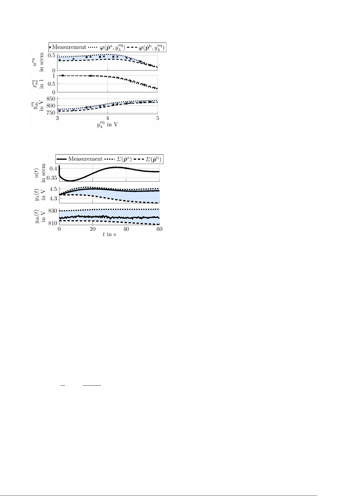
P arameter-in terv al estimation for co op erativ e reactiv e sputtering pro cesses F abian Sc hneider ∗ Christian W¨ olfel ∗ ∗ Chair of Automation, R uhr University Bo chum, Universitaetsstr asse 150, 44801 Bo chum, Germany, { fabian.schneider-v8b, christian.wo elfel } @rub.de Abstract: Reactiv e sputtering is a plasma-based technique to dep osit a thin film on a substrate. This con tribution presents a nov el parameter-in terv al estimation method for a well-established mo del that describ es the uncertain and nonlinear reactive sputtering pro cess b eha viour. Building on a prop osed monotonicity-based mo del classification, the metho d guaran tees that all parameterizations within the parameter in terv al yield output tra jectories and static c haracteristics consisten t with the enclosure induced b y the parameter in terv al. Correctness and practical applicabilit y of the new metho d are demonstrated b y an experimental v alidation, which also rev eals inherent structural limitations of the well-established process mo del for state-estimation tasks. Keywor ds: Nonlinear Analysis, Co operative Systems, Uncertain Systems, Robust Estimation 1. INTR ODUCTION 1.1 Unc ertain nonline ar r e active sputter pr o c esses Reactiv e sputtering is a plasma-based technique used to dep osit thin films on a substrate, for example in the man ufacturing of semiconductors and optical coatings. The pro cess executes in a v acuum cham ber by means of a lo w-pressure plasma. Material is sputtered from the target b y an ion curren t I T (Fig. 1). The resulting metal flo w F m ( t ) to wards the substrate causes the thin film growth. Due to a reactiv e gas in-flow u ( t ), a corresponding partial pressure x rg ( t ) builds up and leads to the formation of com- p ound lay ers characterized by the surface fractions x ta ( t ) and x su ( t ). It is a nonlinear pro cess and the plasma–surface in teraction is uncertain. The state v ariables x ta ( t ), x rg ( t ) are indirectly given b y y sb ( t ) and y λ ( t ), which represent raw sensor signals. Since x su ( t ) is an imp ortan t film-qualit y indicator, reflect- ing the chemical comp osition, but only its steady-state b eha viour x eq su can b e captured by ex-situ measuremen ts, a monitoring problem arises. This concerns the surface b eha viour x su ( t ) during process runtime. Σ ( p ) u ( t ) target x ta ( t ) substrate x su ( t ) x rg ( t ) y sb ( t ) y λ ( t ) x eq su I T F m ( t ) Fig. 1. Material flows in reactiv e sputtering described by the w ell-established pro cess mo del Σ ( p ) (cf. (1)). An in terv al observer can b e systematically designed based on the standard nonlinear process mo del (Berg and Nyb erg, 2005) to giv e guaranteed b ounds on x su ( t ) (Sc hneider and W o elfel, 2023). How ev er, the pro cess mo del is in practice parametrized b y uncertain parameters and, therefore, guaran teed parameter in terv als m ust b e estimated to main tain the guaranteed b ounds of the interv al observer. T o address this estimation task, the presen t contribution in tro duces a no vel metho d, based on a rigorous mono- tonicit y analysis, to systematically determine parameter in terv als for the well-established pro cess mo del (Berg et al., 2014) of reactive sputtering. Its practical applicability for state-estimation tasks is demonstrated by an exp erimen tal v alidation, which also reveals structural limitations of the w ell-established pro cess model. 1.2 Liter atur e survey The standard mo del (Berg and Nyb erg, 2005) for reactive sputtering is based on flow-balance equations for metal, reactiv e gas and comp ound material. Extensions (Kubart et al., 2006; Berg et al., 2014) of the standard mo del incorp orate additional effects, suc h as disso ciation of sputtered molecules and multiple la yers and regions of the surfaces, but they increasingly complicate the design of the in terv al observ er. In the field of plasma and materials science, p oin t v alues for the mo del parameters are identified by an interpla y of differen t metho ds. Kelemen and Madar´ asz (2021) iden tify parameters from analytically obtained prop erties of the static c haracteristics. Sp ecific parameters such as the sputtering yields can b e determined by Monte Carlo sim ula- tions (Mahne et al., 2022). Strijckmans et al. (2012) presen t a metho d for estimating a parameter set guaranteeing a b ounded mo del–output error. These metho ds require This w ork has b een submitted to IF AC for possible publication. substan tial effort or yield parameter estimates of limited accuracy (or both). Bounded-error estimation via set-membership metho ds (Ki- effer and W alter, 2011; Jaulin et al., 2001), suc h as guaran- teed global optimization, set inv ersion via in terv al analysis (SIVIA) and contractor techniques, aim to compute all b o xes in the parameter space that are consistent with a user-defined error b ound b et ween the measuremen ts and mo del output. Monotone dynamical systems, i. e., systems that preserv e the order of their states ov er time (Smith, 1995), facilitate parameter-interv al estimation. Angeli and Son tag (2003) extend the monotonicity concept to con- trolled systems, as is the case in reactive sputtering. Instead of requiring compliance with a user-defined error b ound, this con tribution introduces a new method for estimating t wo parameter v ectors b y constructing enclosing comparison systems and con tracting a predefined parameter searc h domain, thereb y reducing the error betw een the mea- sured data and the mo del output. A rigorous monotonicit y analysis constitutes the basis for the parameter-interv al estimation method. The pro cess model’s monotonicity guaran tees that all parameterizations within the resulting parameter interv al also lead to enclosed mo del outputs, whic h is necessary for interv al-observer design. 1.3 Structur e of the c ontribution Sections 2 and 3 introduce the well-established pro cess mo del and state the ob jectiv es (I) and (I I) of the presen t w ork, resp ectiv ely . The rigorous monotonicity analysis in Sec. 4 addresses ob jective (I), while Sec. 5 presents the new parameter-in terv al estimation method for ob- jectiv e (I I). Sections 6 and 7 presen t the experimental v alidation results and summarize this contribution. 2. ST A TE-SP ACE PROCESS MODEL The well-established first-principles process mo del (Berg et al., 2014) is expressed in the state-space form Σ ( p ) :  ˙ x ( t ) = f ( p , x ( t ) , u ( t )) , x (0) = x 0 y ( t ) = g ( p , x ( t )) . (1) The state x ( t ) = ( x rg ( t ) x ta ( t ) x su ( t ) ) ⊤ and the measured output v ector y ( t ) = ( y λ ( t ) y sb ( t ) ) ⊤ consist of the reactive gas partial pressure, the target surface co verage, the substrate surface cov erage, and the measured raw sensor signals, resp ectiv ely . The system function f and the output function g are given as f 1 ( p , x , u ) = x rg [ − a 11 + a 112 ( x ta − 1) + a 113 ( x su − 1)] + a 12 x ta − a 123 x ta (1 − x su ) + bu (2a) f 2 ( p , x ) = a 212 x rg [1 − x ta ] − a 22 x ta (2b) f 3 ( p , x ) = a 313 x rg [1 − x su ] + a 323 x ta [1 − x su ] − ( a 33c x ta + a 33m [1 − x ta ]) x su (2c) and y λ = g 1 ( p , x rg ) = − c 11 ln ( c 12 x rg ) (3a) y sb = g 2 ( p , x ta ) = c 20 − c 21 x ta . (3b) Assem bling the physically interpretable mo del parameters of Berg et al. (2014) into the parameter vector p = ( a 11 a 112 a 113 a 12 a 123 a 212 a 22 ) ⊤ ( a 313 a 323 a 33c a 33m b c 1l c 12 c 20 c 21 ) ⊤ ! , (4) results in (4) ha ving no direct ph ysical in terpretation. Ho wev er, the constraints implied by the physical in ter- pretation carry o ver to the new parameter space, whic h defines the p ermissible codomains D x = { x ∈ R 3 ≥ 0 | x rg ≤ x rg , max , x ta ≤ 1 , x su ≤ 1 } , D u = R ≥ 0 , D p = { p ∈ R 16 ≥ 0 | a 12 ≥ a 123 , a 33m ≥ a 33c , c 12 x rg , max < 1 } , D y = { y ∈ R 2 ≥ 0 | y = g ( p , x ) , p ∈ D p , x ∈ D x } , for x ( t ), u ( t ), p and y ( t ). Σ ( p ), with p b eing a physically constrained parameter vector, represen ts not a single mo del, but a class of systems determined by the admissible parameter v alues c haracterizing reactive sputtering. Both the dynamic b eha viour of Σ ( p ) and the static c harac- teristics of Σ ( p ) are analysed with regard to monotonicity and are used for the estimation metho d (Sec. 5). Solv- ing 0 = f ( p , x eq , u eq ) yields the static characteristics u eq = π u ( p , x eq rg , x eq ta , x eq su ) (5a) = − 1 b ( a 12 x eq ta − x eq 123 x eq ta (1 − x eq su ) + x eq rg ( − a 11 + a 112 ( x eq ta − 1) + a 113 ( x eq su − 1))) x eq su = π su ( p , x eq rg , x eq ta ) (5b) = a 313 x eq rg + a 323 x eq ta a 313 x eq rg + a 323 x eq ta + a 33c x eq ta + a 33m (1 − x eq ta ) x eq ta = π ta ( p , x eq rg ) = a 212 x eq rg a 212 x eq rg + a 22 . (5c) By comp osing functions (5a) – (5c), the static characteristic π ( p , x eq rg ) =   π u ( p , x eq rg , π 2 ( p , x eq rg ) , π 3 ( p , x eq rg )) π ta ( p , x eq rg ) π su ( p , x eq rg , π 2 ( p , x eq rg ))   = u eq x eq ta x eq su ! (6) is determined for all x eq rg ∈ D x and p ∈ D p . Based on (6) and the in verses x rg = g − 1 1 ( p , y λ ) = 1 c 12 e − y λ c 11 (7a) x ta = g − 1 2 ( p , y sb ) = c 20 − y sb c 21 (7b) of (3a) and (3b) with resp ect to the state v ariables, the measurable steady-state v alues can b e determined from the static c haracteristic φ ( p , y eq λ ) =  u eq x eq su y eq sb  ⊤ (8) of Σ ( p ) for all y eq λ ∈ D y and p ∈ D p . Berg and Nyb erg (2005) sho w the t ypical S-shap ed (non-monotone) static c haracteristic of Σ ( p ). 3. PR OBLEM FORMULA TION 3.1 Notation and pr eliminaries on monotonicity 1 denotes a column vector of ones. F or a vector x , diag ( x ) denotes the diagonal matrix with the entries of x on its diagonal. Sup erscripts “a” and “b” mark parameters and signals that form corresp onding counterparts (see Fig. 2a and 2b). The sign function sign ( f ( · )) ev aluates if f ( · ) is nonnegative (+), nonp ositiv e ( − ) or zero for all considered arguments ( · ). Inequalities such as ≤ and ≥ are in terpreted element-wise when applied to v ectors. A partial order relation, with p ossibly mixed monotonicit y directions, is defined as x a ⪯ r x b ⇐ ⇒ diag ( r ) ( x a − x b ) ≤ 0 Σ ( p ) x a 0 Σ ( p ) x b 0 y a ( t ) y b ( t ) u a ( t ) u b ( t ) (a) Ordered initial conditions (10), ordered manipulated signals (11), with the same parameterization p . Σ ( p a ) x 0 Σ ( p b ) x 0 y a ( t ) y b ( t ) u ( t ) u ( t ) (b) Ordered parameterizations (9), with the same initial condition x 0 and the same input signal u ( t ). Fig. 2. Ordered quantities of a (parameter-) monotone system lead to ordered output tra jectories (12). b y a vector r with en tries r i ∈ { + , 0 , −} . F or exam- ple, x a 1 ≤ x b 1 , x a 2 ≥ x b 2 ⇐ ⇒ x a ⪯ r x b , r = ( + − ) ⊤ . A mapping y = f ( x ) is called monotone with r esp e ct to ⪯ r if from x a ⪯ r x b follo ws y a ≤ y b . L emma 1 ( Monotone function ). Consider a c ontinuously differ entiable function f : D x ⊆ R n → R . If sign  ∂ f ∂ x ( x )  = r ∀ x ∈ D x , then f is monotone with r esp e ct to ⪯ r , cf. (Rudin, 1976, p. 108). 3.2 Obje ctives (I) An analysis is p erformed (Sec. 4) to determine partial order relations ⪯ r p , ⪯ r x , ⪯ r u , ⪯ r y , ⪯ r φ , such that ordered parameters, initial conditions and manipulated signals p a ⪯ r p p b (9) x a 0 ⪯ r x x b 0 (10) ∀ t ≥ 0 : u a ( t ) ⪯ r u u b ( t ) (11) out of their resp ectiv e domains D p D x and D u lead to ordered corresponding state tra jectories ∀ t ≥ 0 : y a ( t ) ⪯ r y y b ( t ) . (12) F urthermore, (9) – (11) in conjunction with (cf. Remark 1) c a 11 = c b 11 , c a 12 = c b 12 (13) m ust ensure ordered corresp onding static characteristics ∀ y eq λ ∈ D y : φ ( p a , y eq λ ) ⪯ r φ φ ( p b , y eq λ ) . (14) (I I) The ob jective of the new parameter-interv al estimation metho d (Sec. 5) is to estimate tw o non-trivial parame- terizations, satisfying (9), such that the measured tra jec- tory y M ( t ) and the measured steady-state v alues φ M ( y eq λ ) are enclosed: ∀ t ≥ 0 : y a ( t ) ⪯ r y y M ( t ) ⪯ r y y b ( t ) (15) ∀ y eq λ ∈ D y : φ ( p a , y eq λ ) ⪯ r φ φ M ( y eq λ ) ⪯ r φ φ ( p b , y eq λ ) . (16) 4. MONOTONICITY ANAL YSIS 4.1 Se ction overview This section addresses ob jectiv e (I) by classifying Σ ( p ) with resp ect to its monotonicit y - b oth for fixed param- eters (Sec. 4.2, Fig. 2a) and with resp ect to parameter v ariations (Sec. 4.3, Fig. 2b). The partial order relations in (9) – (14) are chosen to align increases in parameter v alues (in the sense of ⪯ r p ) with the mo del’s inherent monotonicit y direction ( ⪯ r x , ⪯ r u , ⪯ r y , ⪯ r φ ). x rg u x ta x su y sb y λ + + + + − − r x r y r u (parameter) monotone system function (2) (parameter) monotone output function (3) Fig. 3. Structure graph of Σ ( p ) indicating monotonically increasing (+) and monotonically decreasing (-) cou- plings b etw een u ( t ) and x ( t ) (Lemmas 3 and 6) and b et w een x ( t ) and y ( t ) (Lemmas 2 and 5). 4.2 Monotonicity under fixe d p ar ameterization First, the monotonicit y of Σ ( p ) under fixed parameteriza- tions is analysed, i. e., the implication from (10) and (11) to (12) and (14). L emma 2 ( Monotone output function ). F or al l p ∈ D p and al l ve ctors x a 12 , x b 12 ∈ D x of the first two state variables that c orr esp ond to y a , y b ∈ D y , the output function (3) and its inverse (7) ar e monotone de cr e asing, i. e. x a 12 ≤ x b 12 ⇐ ⇒ y a ⪯ r y y b , (17) with r y = ( − − ) ⊤ . (18) Pro of. Summarize (3a), (3b), (7a) and (7b) by g 12 and g − 1 12 . The equiv alence in (17) is verified by deter- mining the sign pattern  − 0 0 −  = sign ∂ ∂ x 12 g 12 ( p , x 12 ) = sign ∂ ∂ y g − 1 12 ( p , y ) of the gradients of (3) and of (7) and by applying Lemma 1. 2 Lemma 2 addresses the monotonicity of an algebraic equation. In contrast, the dynamical system (1) is called monotone (Smith, 1995; Angeli and Son tag, 2003) if a partial order of the state v ariables is preserv ed ov er time: ∀ t ≥ 0 : x a 0 ⪯ r x x b 0 , u a ( t ) ⪯ r u u b ( t ) = ⇒ x a ( t ) ⪯ r x x b ( t ) . (19) A c o op er ative system is a sp ecial case of a monotone system (Angeli and Sontag, 2003) for r x = + 1 , r u = +1 . (20) L emma 3 ( Co op er ative class of systems Σ ( p )). R e active sputter pr o c esses describ e d by the class of systems Σ ( p ) ar e c o op er ative for al l p ∈ D p , x 0 ∈ D x , u ( t ) ∈ D u , t ≥ 0 . Pro of. sign ∂ ∂ x f ( p , x , u ) = − + + + − + + + − ! , sign ∂ ∂ u f ( p , x , u ) = ( + 0 0 ) ⊤ are constant ∀ p ∈ D p and satisfy Proposition I II.2 in Angeli and Sontag (2003), from which it follows that Σ ( p ) is coop erative. 2 The partial order relations (18) and (20) (Lemmas 2 and 3, Fig. 3) show that the state v ariables p ositiv ely influence eac h other, e. g., increasing the reactive gas partial pressure x eq rg x eq su x eq ta u eq y eq sb y eq λ + + ∗ − − r y e r π partially monotone static c haracteristic (6) monotone output function (3) Fig. 4. e r π , r y represen t monotonically increasing (+) and monotonically decreasing (-) couplings in the structure graph of the static characteristic (14). and the target cov erage increases the substrate cov erage, and that the sensors are suitable as they yield a one-to-one corresp ondence with the first tw o state v ariables. Co operativity do es not imply that the static characteris- tic (6) is monotone in x eq rg as w ell. L emma 4 ( (Non-)Monotone static char acteristic ). The static char acteristic (6) is monotone with r esp e ct to e r π = ( 0 + + ) ⊤ for al l p ∈ D p and x eq rg ∈ D x , i. e., x eq , a rg ≤ x eq , b rg = ⇒  x eq , a ta x eq , a su  ⊤ ⪯ e r π  x eq , b ta x eq , b su  ⊤ . F or some p ∈ D p , the monotonicity of the first r ow of (6) , i. e., x eq rg 7→ u eq , is undefine d. Pro of. The pro of follows the same line of reasoning as the pro of of Lemma 2 by determining sign ∂ ∂ x eq rg π ( p , x eq rg ) = ( ∗ + + ) ⊤ . The mapping x eq rg 7→ u eq is not monotone, since the sign of the first row is not constant (denoted b y ∗ ) for all x eq rg ∈ D x and p ∈ D p , which results from sign ∂ ∂ x π u ( p , x eq rg , x eq ta , x eq su ) = ( + − − ) ⊤ . 2 The non-monotonicity of x eq rg 7→ u eq (Fig. 6) o ccurs b ecause increasing x eq rg increases the target co verage, reduces the sputtering rate and substrate reactiv e gas consumption and th us a smaller reactive gas inflow u eq is needed to maintain the same x eq rg . This section has shown that Σ ( p ) and (3) are monotone in the sense of (10) – (12) with the partial order relations (18) and (20) (Lemmas 2 and 3) under a fixed parameteri- zation p ∈ D p (Fig. 2a). The non-monotonicity of the static c haracteristic x eq rg 7→ u eq (Lemma 4) constitutes a structural limitation of the parameter-interv al estimation metho d (Sec. 5) with resp ect to the num ber of parameter in terv als that can be estimated (Remark 1). Nevertheless, the relation x eq rg 7→ u eq is monotone with resp ect to parameter v ariations, as shown in the next section. 4.3 Monotonicity with r esp e ct to p ar ameter variations In the following, the monotonicity of Σ ( p ) with resp ect to the parameter v ector p (Fig. 2b) is analysed. L emma 5 ( Par ameter-monotone output function ). Consider (18) , p a , p b ∈ D p and r g p = ( 0 . . . 0 − + − + ) ⊤ . (21) Then, the output function (3) and its inverse (7) ar e monotone in the sense that ∀ x 12 ∈ D x : p a ⪯ r g p p b = ⇒ y a ⪯ r y y b (22) ∀ y ∈ D y : p a ⪯ r g p p b = ⇒ x a 12 ⪯ r y x b 12 . (23) Pro of. F or p ∈ D p , x ∈ D x , y ∈ D y , the col- umn sums of sign ∂ ∂ p g 12 ( p , x ) = sign ∂ ∂ p g − 1 12 ( p , y ) =  0 . . . 0 + − 0 0 0 . . . 0 0 0 + −  are equal to − r g ⊤ p , whic h prov es (22) and (23) according to Lemma 1. 2 In contrast to dynamical-system monotonicit y (cf. (19)), whic h considers different initial conditions and input signals (Fig. 2a), the following definition considers different parameterizations while k eeping the initial conditions and the input signal fixed (Fig. 2b). Definition 1 ( Par ameter-monotone system ). The system (1) is c al le d p ar ameter-monotone with r esp e ct to ⪯ r f p if the implic ation p a ⪯ r f p p b = ⇒ x a ( t ) ≤ x b ( t ) , t ≥ 0 (24) holds for al l p a , p b ∈ D p , x 0 ∈ D x and al l t ≥ 0 : u ( t ) ∈ D u . L emma 6 ( Par ameter-monotone class of systems Σ ( p )). R e active sputter pr o c esses describ e d by the class of sys- tems Σ ( p ) ar e p ar ameter-monotone with r esp e ct to ⪯ r f p with r f p = ( − − − + − + − + + − − + 0 0 0 0 ) ⊤ . (25) Pro of. The system function (2) is monotone with respect to ⪯ r f p , since the column sums of sign ∂ ∂ p f ( p , x , u ) = − − − + − + 0 0 0 0 + − 0 0 0 0 + + − − 0 0 0 0 ! are equal to r f ⊤ p for all p ∈ D p , x ∈ D x , u ∈ D u due to Lemma 1. Considering eac h parameter p i as a constant input signal and applying Corollary I II.3 from Angeli and Sontag (2003) pro ves (24). 2 Lemmas 5 and 6 state that if the parameter vector (4) is increased with resp ect to ⪯ r f p , x ( t ) and y ( t ) increase in the sense of r x and r y monotonously as shown in Fig. 3, i. e., to the same direction as describ ed b y Lemmas 2 and 3. L emma 7 ( Par ameter-monotone static char acteristics ). Consider two p ar ameterizations p a , p b ∈ D p . The static char acteristic (6) is monotone such that for (25) and r π = ( − + + ) ⊤ and al l x eq rg ∈ D x the fol lowing implic ation holds: p a ⪯ r f p p b = ⇒  u a , eq rg x a , eq ta x a , eq su  ⪯ r π  u b , eq rg x b , eq ta x b , eq su  . Pro of. Analogously to the pro ofs of Lemmas 5 and 6, Lemma 7 is prov en with sign ∂ ∂ p π ( p , x eq rg ) = + + + − + − + − − + + − 0 0 0 0 0 0 0 0 0 + − 0 0 0 0 0 0 0 0 0 0 0 0 0 0 + − + + − − 0 0 0 0 0 ! . 2 Lemma 7, in conjunction with Lemma 5, states that increasing the parameter v ector p with resp ect to ⪯ r f p leads to an increase in x eq ta and in x eq su , and to a decrease in u eq , in y eq λ and in y eq sb , as illustrated in Fig. 5. x eq rg x eq su x eq ta u eq y eq sb y eq λ + + − − − r y r π parameter-monotone static c haracteristic (6) parameter monotone output function (3) Fig. 5. r π and r y represen t monotonically increasing (+) and monotonically decreasing (-) couplings in the structure graph of the static characteristic (14) for an increase in p in direction r p . 4.4 Main the or em Since no element of p app ears in the system function (2) and concurren tly in the output function (3), r f p ( r g p ) defines no order for the parameters of the output function (system function). Th us, the partial order relation r p = r f p + r g p (26) (cf. (21) and (25)) defines an order for each parameter. The or em 1 ( Monotonicity of the class of systems Σ ( p )). L et p artial or der r elations b e define d by (18) , (20) , (26) , and r φ = ( − + − ) ⊤ . Consider p ar ameter ve ctors p a , p b ∈ D p satisfying (13) , initial c onditions x a 0 , x b 0 ∈ D x and input signals t ≥ 0 : u a ( t ) , u b ( t ) ∈ D u that ar e or der e d ac c or ding to (9) – (11). Then the c orr esp onding output tr aje ctories y a ( t ) , y b ( t ) and static char acteristics φ ( p a , y eq λ ) , φ ( p b , y eq λ ) of the class of systems Σ ( p ) ar e monotone in the sense of (12) and (14) . Pro of. (12) holds, since an increase in the parameter v alues in the sense of (26) has the same monotone influence on x ( t ) and on y ( t ) (Lemmas 5 and 6) as x 0 and u ( t ) (Lemmas 2 and 3). Due to (13), the same static reactive gas partial pres- sure x eq rg = x eq , a rg = x eq , b rg results for p a and p b , whic h renders Lemma 7 applicable such that (6) is ordered according to ⪯ r π . Due to Lemmas 2 and 5, (3b) increases if p increases with resp ect to (26) and to (18), (8) is monotone with resp ect to r φ and (14) holds true. 2 R emark 1. The exact mapping (7a) fr om y eq λ to x eq rg , r esulting fr om (13) , is ne c essary to obtain the or der e d static char acteristic (14) . Violation of (13) le ads to differ ent values x eq , a rg and x eq , b rg for one me asur e d y eq λ , and due to the undefine d monotonicity of x eq rg to u eq (L emma 4), it is not p ossible to determine the or der r elation for the first element of r φ . Thus, no intervals for c 11 and c 12 c an b e estimate d. 5. P ARAMETER-INTER V AL ESTIMA TION METHOD This section addresses ob jective (I I) and presen ts the new metho d to determine t w o parameterizations p a and p b that, firstly , fulfil the inclusion requirement (9) with resp ect to the parameter vector and, secondly , ensure the inclusion requiremen ts (15) and (16) of the measured steady-state v alues φ M ( y eq λ ) and the measured output tra jectory y M ( t ). Thereto, the t wo optimization problems ˆ p a = argmin p a ∈ D a p J ( p a ) , ˆ p b = argmin p b ∈ D b p J ( p b ) sub ject to (15) and (16) (27) ha ve to b e solved. Based on the relative change δ of a nominal parameter v ector p 0 whose v alues can b e taken from literature and on the constraints in (13), a b o x D 0 p =  p ∈ [(1 − δ ) p 0 , (1 + δ ) p 0 ] | c 11 = c 0 11 , c 12 = c 0 12  (28) is defined as the search domain for the parameter vectors. T o guarantee that the parameter v alues are increased and decreased according to the partial order relation (9), the searc h domain D 0 p is split in to disjunct sets D a p =  p ∈ D 0 p | p ⪯ r p p 0  , D b p =  p ∈ D 0 p | p 0 ⪯ r p p  . (29) The cost function J ( p ) = J y ( p ) + J φ ( p ) consists of J φ ( p ) = 3 X q =1 K φ q X k =1  φ M q ( y eq λ ( k )) − φ q ( p , y eq λ ( k )) | {z } ∆ φ q ( k )  2 w φ q ( k ) J y ( p ) = 2 X q =1 K y q X k =1  y M q ( k T ) − y q ( p , k T ) | {z } ∆ y q ( k )  2 w y q ( k ) (30) and corresponds to the elemen t-wise weigh ted (cf. w φ q ( k ), w y q ( k )) l 2 -norm of the differences ∆ φ q ( k ), and ∆ y q ( k ) b e- t ween the measured data and the mo del data. In (30), y q ( p , t ) denotes the solution of Σ ( p ) for the manipulated signal u ( t ) = u M ( t ) used in the exp erimen t and the initial condition x 0 = x eq that is equal to the equilibrium state (cf. (6)) for the initially measured voltage y M λ (0). K φ q and K y q denote the num b er of measured equilibrium states and the num b er of sampling p oin ts obtained with sampling time T . The argument k denotes the resp ectiv e element in the data series. Although the optimization problems in (27) are non-con vex, J ( p ) is monotone increasing (decreasing) with resp ect to ⪯ r p for all p ∈ D a p ( D b p ) and, therefore, (27) yields monotonic optimization problems. Solving (27) con tracts (28) to the interv al defined by ˆ p a and ˆ p b and guarantees the fulfilling of ob jective (I I) of the parameter-in terv al estimation method: the parameter searc h domains in (29) ensure (9), the monotonicit y of the static c haracteristic, i. e., y eq λ 7→ x eq , (Fig. 4 and 5) ensures (10), the condition (11) holds, since u M ( t ) is used for both mo dels as input and (15) and (16) hold b ecause they are included as constraints in (27). The parameter-in terv al estimation method is summarized b y the following algorithm. Giv en are a nominal parameter vector p 0 and m easure- men ts of the steady-state v alues φ M ( y eq λ ) and of a tra jectory tuple ( u M ( t ) , y M ( t )). 1. Select a small δ and determine p a = diag ( 1 − δ r p ) p 0 and p b = diag( 1 + δ r p ) p 0 with the restriction (13). 2. V erify that (15) and (16) hold true, otherwise in- crease δ and go back to step 1. 3. Select non-zero w eights w φ q ( k ), w y q ( k ) and solve (27). The result is tw o parameterizations ˆ p a and ˆ p b guaran tee- ing the inclusion prop erties (15) and (16) and that ev ery Fig. 6. The mo del output provides an enclosure for the measured steady-state v alues. Fig. 7. A t ypical measured tra jectory enclosed b y the mo del output defined by tw o parameter vectors obtained from (27). parameter vector (4) satisfying ˆ p a ⪯ r p p ⪯ r p ˆ p b yields a static characteristic (8) and output tra jectory y ( t ) that b oth are also enclosed in the sense of (15) and (16). 6. EXPERIMENT AL V ALIDA TION The optimization problems in (27) are solved, based on measuremen ts of the steady-state v alues φ M ( y eq λ ) and of m ultiple step resp onses ( u M ( t ), y M ( t )). x eq su is measured b y energy disp ersive X-ray sp ectroscop y after unloading the coated substrate of the reactor cham b er. Figures 6 and 7 demonstrate the practical applicabilit y and the correctness of the parameter-interv al estimation metho d, since the measured data is enclosed by the re- sp ectiv e model output data for the t wo parameteriza- tions ˆ p a and ˆ p b . The av erage relative parameter-interv al width 0 . 08 = 1 16 P 16 i =1 | ˆ p b i − ˆ p a i | 2 | ˆ p b i + ˆ p a i | sho ws that the estimation metho d is able to determine a tight parameter in terv al for the wide range of y eq λ depicted in Fig. 6. Due to Theorem 1, ev ery parameter vector p satisfying ˆ p a ⪯ r p p ⪯ r p ˆ p b leads to static characteristics and output tra jectories that are enclosed b y the interv al depicted in Fig. 6 and 7. If additional equilibrium p oints with y eq λ < 3 V , or output tra jectories spanning more than 0 . 5 V, are tak en into accoun t, excessively large parameter interv als m ust b e allo wed by δ (cf. (28)) and result from (27). This suggests that the mo del’s structural v alidit y is confined to regions around specific op erating p oin ts. 7. CONCLUSION This con tribution classifies the well-established process mo del of reactiv e sputtering as co op erativ e and parameter- monotone. Based on this result, a nov el parameter-interv al estimation metho d is introduced that provides a guaran- teed enclosure of the measurements. Exp erimen tal results demonstrate its correctness and practical applicability . The metho d enables the determination of a parameter set that allo ws the design of an interv al observer contributing to the monitoring task for reactive sputtering. F uture work will inv estigate more sophisticated process mo dels and generally informative plasma v ariables, aiming, e. g., to further reduce the parameter in terv al width. A CKNOWLEDGEMENTS The authors gratefully ackno wledge financial supp ort from the Deutsche F orsch ungsgemeinschaft (DFG) through gran t 562363182. REFERENCES Angeli, D. and Sontag, E.D. (2003). Monotone control systems. IEEE T r ans. on Automatic Contr ol , 48(10), 1684–1698. Berg, S. and Nyb erg, T. (2005). F undamental understand- ing and mo deling of reactive sputtering pro cesses. Thin Solid Films , 476(2), 215–230. Berg, S., S¨ arhammar, E., and Nyb erg, T. (2014). Upgrading the “Berg-mo del” for reactive sputtering pro cesses. Thin Solid Films , 565, 186–192. Jaulin, L., Kieffer, M., Didrit, O., and ´ Eric W alter (2001). Applie d Interval A nalysis . Springer. Kelemen, A. and Madar´ asz, R.R. (2021). Reactiv e mag- netron sputtering: an offline parameter iden tification metho d. In IEEE Int. Symp osium on Applie d Computa- tional Intel ligenc e and Informatics , 357–362. Kieffer, M. and W alter, E. (2011). Guaranteed estimation of the parameters of nonlinear contin uous-time mo dels: Con tributions of interv al analysis. Int. J. of A daptive Contr ol and Signal Pr o c essing , 25(3), 191–207. Kubart, T., Kapp ertz, O., Nyb erg, T., and Berg, S. (2006). Dynamic behaviour of the reactive sputtering pro cess. Thin Solid Films , 515(2), 421–424. Mahne, N., ˇ Cek ada, M., and Panjan, M. (2022). T otal and differen tial sputtering yields explored b y SRIM sim ulations. Co atings , 12(10). Rudin, W. (1976). Principles of Mathematic al Analysis . McGra w-Hill, 3rd edition. Sc hneider, F. and W oelfel, C. (2023). Robust interv al observ er for substrate state estimation of nonlinear reactiv e sputter pro cesses. In Pr o c. of the IEEE Conf. on Contr ol T e chnolo gy and Applic ations , 194–200. Smith, H.L. (1995). Monotone Dynamic al Systems . Ameri- can Mathematical Society . Strijc kmans, K., Lero y , W., De Gryse, R., and Depla, D. (2012). Mo deling reactiv e magnetron sputtering: Fixing the parameter set. Surfac e and Co atings T e chnolo gy , 206(17), 3666–3675.