Structure-Preserving Integration for Magnetic Gaussian Wave Packet Dynamics
We develop structure-preserving time integration schemes for Gaussian wave packet dynamics associated with the magnetic Schrödinger equation. The variational Dirac--Frenkel formulation yields a finite-dimensional Hamiltonian system for the wave packe…
Authors: Sebastian Merk, Caroline Lasser
STR UCTURE-PRESER VING INTEGRA TION F OR MA GNETIC GA USSIAN W A VE P A CKET D YNAMICS ∗ SEBASTIAN MERK † AND CAROLINE LASSER † † Abstract. W e develop structure-preserving time integration sc hemes for Gaussian wa ve pac ket dynamics associated with the magnetic Schr¨ odinger equation. The v ariational Dirac–F renkel for- mulation yields a finite-dimensional Hamiltonian system for the wa ve pack et parameters, where the presence of a magnetic vector p otential leads to a non-separable structure and a mo dified symplec- tic geometry . By in tro ducing kinetic momenta through a minimal substitution, we reform ulate the av eraged dynamics as a Poisson system that closely parallels the classical equations of charged par- ticle motion. This representation enables the construction of Boris-type integrators adapted to the v ariational setting. In addition, we propose explicit high-order symplectic schemes based on splitting methods and partitioned Runge–Kutta in tegrators. The proposed methods conserv e the quadratic inv ariants c haracterizing the Hagedorn parametrization, preserve linear and angular momen tum un- der symmetry assumptions, and exhibit near-conserv ation of the av eraged Hamiltonian o ver long time interv als. Rigorous error estimates are derived for b oth the wa ve pack et parameters and observable quantities, with bounds uniform in the semiclassical parameter. Numerical exp eriments demonstrate the fav orable long-time behavior and structure preserv ation of the integrators. Key words. Gaussian w a ve pack ets; magnetic Schr¨ odinger equation; structure-preserving in te- grators; symplectic metho ds; Hamiltonian systems; long-time integration. MSC co des. 65P10, 81Q05, 37M15, 81S30, 78A35 1. In tro duction. The time-dependent Sc hr¨ odinger equation with electromag- netic p otential arises in a wide range of applications, including molecular dynamics, c harged particle transp ort, and plasma ph ysics. Here, we consider the ev olution in semiclassical scaling, (1.1) iε∂ t ψ ( t ) = H ( t ) ψ ( t ) , ψ ( t 0 ) = ψ 0 , with Hamiltonian op erator (1.2) H ( t ) = 1 2 |− iε ∇ x − A ( t, x ) | 2 + V ( t, x ) , x ∈ R d , and semiclassical parameter ε > 0. In the presence of a magnetic field, the Hamil- tonian in volv es a vector potential A ( t, · ) and a scalar potential V ( t, · ), which leads to non-separable dynamics with additional geometric structure. Accurate long-time sim ulation of suc h systems requires n umerical metho ds that respect fundamental in- v ariants suc h as symplecticity , linear and angular momentum conserv ation, and near- conserv ation of energy . In the high-dimensional and/or highly-oscillatory regime, Gaussian wa ve pack et metho ds pro vide an efficien t reduced description of the dynamics by approximating the solution through parametrized families of localized states [8, 3, 10]. V ariational form ulations based on the Dirac–F renk el principle lead to closed systems of ordi- nary differen tial equations that retain essenti al geometric prop erties of the underlying Sc hr¨ odinger dynamics. If the wa v e pac ket parameters are chosen in Hagedorn’s pa- rametrization, then the approximate evolution has canonical Hamiltonian structure, whic h forms the basis of man y successful semiclassical appro ximations [17, 16, 11]. ∗ F unding: F unded by the Deutsche F orsch ungsgemeinschaft (DFG, German Researc h F ounda- tion) – TRR 352 – Pro ject-ID 470903074. † Department of Mathematics, T ec hnical Univ ersity of Munic h, German y (s.merk@tum.de, classer@tum.de). 1 2 SEBASTIAN MERK, CAROLINE LASSER F or nonmagnetic quantum dynamics ( A = 0), structure-preserving time integra- tors for Gaussian wa ve pack et dynamics hav e been prop osed in [4, 15]. By preserv ation of the wa ve pack et induced P oisson structure, linear and angular momen ta are con- serv ed, and energy has a fa vorable long-time b ehavior. In con trast, the presence of magnetic fields ( A = 0) introduces additional coupling through the vector potential, whic h leads to non-separable Hamiltonians and modified symplectic prop erties. While v ariational Gaussian appro ximations for the magnetic Sc hr¨ odinger equation hav e re- cen tly been deriv ed and analyzed in the contin uous-time setting [10, 2], the Boris-t yp e in tegrator proposed in [20] app ears to b e the only structure-adapted time discretiza- tion for magnetic v ariational Gaussian dynamics. A rigorous error analysis of this metho d, how ever, has not y et b een established. The present work develops a framew ork for structure-preserving time integration sc hemes for Gaussian w av e pac ket dynamics in the presence of magnetic fields. B y expressing the v ariational equations of motion in canonical co ordinates, we construct a veraged p oten tials A ( t, q ) and V ( t, q ) and then a parameter Hamiltonian h ( t, q , p ) = 1 2 p ⊤ p − p ⊤ A ( t, q ) + V ( t, q ) , that closely parallels the classical Hamiltonian of charged particle dynamics. Intro- ducing kinetic momenta through a minimal substitution, we then derive a P oisson form ulation for the parameter evolution. This reformulation enables the construction of a staggered-grid Boris in tegrator that a v oids the extrapolation step required in [20]. Ho wev er, the new scheme shares the same limitation, namely the lack of preserv ation of the symplecticit y conditions for the w av e pac k et width matrices, and therefore do es not guaran tee square integrabilit y of the v ariational approximation. W e there- fore mo ve beyond Boris-type schemes and design explicit high-order symplectic in te- grators based on splitting tec hniques and partitioned Runge–Kutta metho ds. These sc hemes conserve the quadratic inv arian ts underlying the Hagedorn parametrization, in particular square in tegrability of the wa v e pack et, preserv e linear and angular mo- men tum in the presence of symmetries, and yield near-conserv ation of the av eraged Hamiltonian o ver long time in terv als. Imp ortan tly , all in tegrators can b e implemen ted explicitly despite the non-separable structure of the magnetic Hamiltonian. Rigorous accuracy results are established for b oth the wa ve pac ket parameters and observ able quan tities, with error b ounds that remain uniform in the semiclassical parameter. Numerical exp eriments illustrate the preserv ation of geometric structure and the impro v ed long-time b eha vior compared to non-structure-preserving metho ds. Structure of the pap er. The pap er is organized as follo ws. Section 2 in tro duces the magnetic Schr¨ odinger equation, the Gaussian wa v e pac k et parametrization, and the con tinuous-time v ariational appro ximation. Section 3 derives the Hamiltonian and P oisson form ulations of the v ariational dynamics and establishes conserv ation la ws. Section 4 presents Boris-type and high-order symplectic in tegrators together with their structural prop erties. Section 5 pro vides the proofs for the analysis of accuracy and energy behavior. Numerical experiments are reported in section 6. 2. Magnetic v ariational Gaussians. W e w ork in the Hilb ert space of square in tegrable functions H = L 2 ( R d , C ) and denote the inner product and the induced norm b y ⟨· , ·⟩ and ∥ · ∥ , resp ectiv ely . W e study magnetic Sc hr¨ odinger Hamiltonians of the form (1.2) under the follo wing growth and regularit y assumptions. Assumption 2.1. We supp ose that the sc alar p otential V : R × R d → R and the ve ctor value d p otential A = ( A j ) j =1 ,...,d : R × R d → R d ar e infinitely often differ en- tiable and satisfy the fol lowing c onditions: INTEGRA TION F OR MAGNETIC W A VE P ACKET DYNAMICS 3 (a) V ( t, · ) + 1 2 | A ( t, · ) | 2 is sub quadr atic, i.e., ∇ k V ( t, · ) + 1 2 | A ( t, · ) | 2 is b ounde d for al l k ∈ N d with | k | ≥ 2 . (b) A ( t, · ) and ∂ t A ( t, · ) ar e subline ar, i.e., ∇ k A ( t, · ) , ∇ k ∂ t A ( t, · ) ar e b ounde d for al l k ∈ N d with | k | ≥ 1 . With Assumption 2.1, magnetic Schr¨ odinger dynamics are globally w ell-p osed in H , see e.g. [14, § 5.3] or [21, § 4]. In particular, the norm of the solution ψ ( t ) of the Cauch y problem (1.1) with initial data ψ 0 ∈ H is a conserv ed quantit y , and for time-indep enden t Hamiltonians H ( t ) = H the energy is conserv ed as well, ∥ ψ ( t ) ∥ = ∥ ψ 0 ∥ and ⟨ ψ ( t ) , H ψ ( t ) ⟩ = ⟨ ψ 0 , H ψ 0 ⟩ for all t ∈ R . If the Hamiltonian H ( t ) has further symmetries, then there are more in v ariants, see also subsection 2.3. 2.1. V ariational Gaussian wa ve pack ets. W e appro ximate the quan tum so- lution ψ ( t ) ≈ u ( t ) by a complex Gaussian w a v e pac ket u ( t ) ∈ M with M = u ∈ H u ( x ) = exp i ε 1 2 ( x − q ) ⊤ C ( x − q ) + p ⊤ ( x − q ) + ζ , q ∈ R d , p ∈ R d , C = C ⊤ ∈ C d × d , Im C is positive definite , ζ ∈ C . F or a systematic construction of the appro ximation, w e use the Dirac–F renk el v aria- tional principle, iε∂ t u ( t ) = P u ( t ) ( H ( t ) u ( t )) , (2.1) where P u : H → T u M is the orthogonal pro jection on to the tangen t space T u M , whic h can b e iden tified as T u M = { φu | φ is a complex d -v ariate p olynomial of degree at most 2 } , see [11, § 3]. F or structure-preserving integration, it is con v enient to use Hagedorn’s parametrization of a normalized squeezed wa v e pac ket u ∈ M , see [5] and [11, § 4.1]. W e set C = P Q − 1 with Q, P ∈ C d × d in vertible suc h that (2.2) Y = Re Q Im Q Re P Im P is symplectic , that is, Y ⊤ Ω d Y = Ω d for Ω d = 0 Id d − Id d 0 . Using the determinan t of the complex matrix Q for the normalization of the wa ve pac ket, ∥ u ∥ = 1, we then write u ( x ) = ( επ ) − d 4 det( Q ) 1 2 exp i ε 1 2 ( x − q ) ⊤ P Q − 1 ( x − q + p ⊤ ( x − q ) + S with a real phase factor S ∈ R . The Dirac–F renkel principle (2.1) generates a globally w ell-p osed parameter tra jectory t 7→ ( q ( t ) , p ( t ) , Q ( t ) , P ( t ) , S ( t )) such that the corre- sp onding u ( t ) ∈ M is a p ow erful semiclassical approximation of ψ ( t ) with rigorous error estimates, see [12, Theorem 4.4] and [2, Theorem 3.10]. 4 SEBASTIAN MERK, CAROLINE LASSER 2.2. Canonical parameter co ordinates. The magnetic Sc hr¨ odinger Hamil- tonian can b e seen as a semiclassically scaled pseudo-differen tial op erator in W eyl- quan tization, H ( t ) = op( h ( t )), with classical sym b ol h ( t, x, ξ ) = 1 2 | ξ − A ( t, x ) | 2 + V ( t, x ) , ( x, ξ ) ∈ R 2 d , see Lemma A.2. This allo ws to write the energy exp ectation v alue as a phase space in tegral w eighted with the state’s Wigner function, ⟨ ψ , H ( t ) ψ ⟩ = Z R 2 d h ( t, ζ ) W ψ ( ζ ) dζ , ψ ∈ H . F or a complex Gaussian wa ve pack et u ∈ M , the Wigner function is a p ositive phase space Gaussian, W u ( ζ ) = (2 π ) − d det(Σ ε ) exp − 1 2 ( ζ − z ) ⊤ Σ − 1 ε ( ζ − z ) , ζ ∈ R 2 d , with cen ter z = ( q , p ) ∈ R 2 d and p ositiv e definite co v ariance matrix Σ ε = Y ( ε ) Y ( ε ) ⊤ defined by Y ( ε ) = r ε 2 Y = p ε 2 Re Q p ε 2 Im Q p ε 2 Re P p ε 2 Im P , see Lemma A.1 or [18]. If we v ectorize these parameters w e get a 2 D -dimensional phase space with 2 D = 2( d + 2 d 2 ) canonical co ordinates q := q p ε 2 v ec(Re Q ) p ε 2 v ec(Im Q ) , p := p p ε 2 v ec(Re P ) p ε 2 v ec(Im P ) . (2.3) More generally , if A = op( a ) is a linear op erator A : D ( A ) → H with smo oth W eyl- sym b ol a : R 2 d → C and if there exists β k > 0 such that ∂ k a ( z ) ≤ C k exp( β k ∥ z ∥ 2 ) , (2.4) for all k ∈ N 2 d and z ∈ R 2 d , then we can write a Gaussian a verage ⟨ a ⟩ u := ⟨ u, A u ⟩ as ⟨ a ⟩ u = Z R 2 d a ( ζ ) W u ( ζ ) dζ = (2 π ) − d Z R 2 d a (Y ( ε ) ζ + z ) exp − 1 2 ζ ⊤ ζ dζ . (2.5) W e therefore consider the av erage ⟨ a ⟩ u as a nonlinear function R 2 D → C , z = ( q , p ) 7→ ⟨ a ⟩ u or equiv alently ( z, Y ( ε ) ) 7→ ⟨ a ⟩ u ; the last equalit y in the definition of the av erage sho ws that their ε -dependence comes only through the cov ariance factor Y ( ε ) . INTEGRA TION F OR MAGNETIC W A VE P ACKET DYNAMICS 5 2.3. Linear and quadratic in v ariants. If the p otentials A ( t, · ) and V ( t, · ) ha ve translational (or rotational) symmetries, then the classical system ˙ q = p − A, ˙ p = ∇ q A ⊤ p − ∇ q V conserv es the total linear (or angular) momentum; this generalizes to the v ariational parameters as sho wn for the electric Sc hr¨ odinger equation in [4, § 4] and extended to the magnetic case in [16, § 4]. There, also a semiclassical angular momentum is in tro duced, see [16, eq.(27)], L ε = pq ⊤ − q p ⊤ + ε 2 Re( P Q ∗ − QP ∗ ) . All this can be form ulated in terms of the v ectorized coordinates ( q , p ), if the p oten- tials are inv ariant as follo ws. T r anslation invariant. Then the linear momentum P d j =1 p j is conserved, w hic h can b e written as a linear inv ariant in p . R otation invariant. Then the semiclassical angular momen tum L ε is conserv ed, whic h can be written as a mixed quadratic in v ariant in q and p . Indeed, L ε is uniquely defined by its action on skew-symmetric matrices K ∈ R d × d , L ε ( K ) = 1 2 tr L ⊤ ε K = p ⊤ K q + ε 2 Re (tr( P ∗ K Q )) = p ⊤ K q + ε 2 Re (v ec( P ) ∗ (Id d ⊗ K )v ec( Q )) = p ⊤ K Id d ⊗ K Id d ⊗ K q , where the last equation uses Kronec k er product calculus, see e.g. [22, Ch. 2]. Moreo ver, the symplecticit y condition (2.2) for the matrix Y can also b e viewed as a mixed quadratic form. F or example, examining its top-left block, we write E ( j,k ) = ( e j e ⊤ k − e k e ⊤ j ) ⊗ Id d with j, k = 1 , . . . , d to get Re( Q ) ⊤ Re( P ) − Re( P ) ⊤ Re( Q )) j k = v ec(Re Q ) ⊤ v ec(Im Q ) ⊤ E ( j,k ) − E ( j,k ) v ec(Re P ) v ec(Im P ) . Rewriting the other blo c ks similarly , w e can define a family of matrices I k ∈ R D × D suc h that (2.2) is equiv alent to (2.6) q ⊤ I k p = v ec(Ω) k , k = 1 , . . . , 4 d 2 . 3. Con tin uous-time results. W e start by presenting our k ey observ ation on deriv atives of av erages with resp ect to the v ectorized parameters z and Y ( ε ) , that go vern the phase space center and the complex width of a Gaussian u ∈ M . W e hav e the following tw o striking relations. Theorem 3.1 (Deriv ativ e formulas). L et A = op( a ) b e an observable with smo oth symb ol a that satisfies the gr owth assumption (2.4) , then ∇ z ⟨ a ⟩ u = ⟨∇ ζ a ⟩ u and ∇ Y ( ε ) ⟨ a ⟩ u = ⟨∇ ζ ∇ ⊤ ζ a ⟩ u Y ( ε ) . Pr o of. The pro of can b e found in subsection 5.1. This is the primary tool for deriving the Hamiltonian structure, and it is also practi- cally helpful, as we used it with automatic differen tiation routines to provide a fully flexible wa v e pac ket integrator for the numerical exp eriments in se ction 6. 6 SEBASTIAN MERK, CAROLINE LASSER 3.1. General Hamiltonian dynamics. The combination of the abov e tw o de- riv ative identities with the canonical parametrization z = ( q , p ) introduced in (2.3) rev eals sev eral structural properties of the v ariational approximation that are not immediately apparent. F or their dev elopmen t, w e adopt a general Hamiltonian p er- sp ectiv e and view the magnetic Sc hr¨ odinger op erator (1.2) as a sp ecial case of a linear op erator satisfying the following set of assumptions. Assumption 3.2. We supp ose that the Weyl-symb ol h ( t, · ) of the Hamiltonian op er ator H ( t ) = op( h ( t, · )) is smo oth, satisfies the exp onential gr owth assumption (2.4) , and sub quadr atic gr owth, i.e., ther e exist C k ( t ) ∈ L 1 loc such that ∂ k z h ( t, z ) ≤ C k ( t ) for z ∈ R 2 d and | k | ≥ 2 . Under these assumptions, the Cauch y problem (1.1) is well-posed in H , see e.g. [14, § 5.6]. F or suc h general Hamiltonian op erators, [2, § 3] established well-posedness of the v ariational appro ximation u ( t ) ∈ M and derived the equations of motion for the parameters ( q , p, Q, P , S ); using the canonical parameter coordinates ( q , p ) introduced in (2.3), these results can b e reco v ered in a concise and transparen t manner. These w ell-p osedness results can also be established for Hamiltonians with co ercive sym b ols, due to the existence of the classical flo w. Corollar y 3.3 (Equations of motion). Under Assumption 3.2 c onsider the variational wave p acket appr oximation u ( t ) ∈ M . Then, the e quations of motion for the c anonic al p ar ameters z ( t ) ar e given by Hamilton ’s e quations ˙ z ( t ) = Ω D ∇ z h ( t, z ( t )) . (3.1) for the aver age d Hamiltonian h ( t, z ( t )) := ⟨ h ( t, · ) ⟩ u ( t ) . Pr o of. The pro of can b e found in subsection 5.2. R emark 3.4. The phase S ( t ) of the w av e pack et u ( t ) evolv es similarly to the classical action of the system: Using the equation deriv ed in [2, eq. 3.4d] and the phase change of the determinant, we get d dt S ( t ) + ε 4 Re tr( P ( t ) Q ( t ) ∗ ) = p ( t ) ⊤ ˙ q ( t ) − h ( t ) . (3.2) Global well-posedness of the v ariational dynamics is straightforw ard due to the follo wing Corollary . Corollar y 3.5 (W ell-p osedness). Under Assumption 3.2 c onsider the varia- tional wave p acket appr oximation u ( t ) ∈ M . Then, the variational Hamiltonian h ( t, · ) : R 2 D → R , h ( t, · ) = ⟨ h ( t, · ) ⟩ u ( t ) inherits the sub quadr atic gr owth or the c o er civity of the classic al Hamiltonian symb ol h ( t, · ) : R 2 d → R . In p articular, the variational e quations of motion (3.1) ar e glob al ly wel l-p ose d. Pr o of. The pro of can b e found in subsection 5.2. 3.2. Magnetic dynamics. F or the magnetic Hamiltonian (1.2), the v ariational Hamiltonian of Corollary 3.3 tak es the form h ( t, q , p ) = 1 2 p ⊤ p − p ⊤ A ( t, q ) + V ( t, q ) , (3.3) INTEGRA TION F OR MAGNETIC W A VE P ACKET DYNAMICS 7 with av eraged p otentials A ( t, q ) := ⟨ A ( t, · ) ⟩ u v ec ⟨ J A ( t, · ) ⟩ u p ε 2 Re Q v ec ⟨ J A ( t, · ) ⟩ u p ε 2 Im Q , (3.4) V ( t, q ) := 1 2 ⟨| A ( t, · ) | 2 ⟩ u + ⟨ V ( t, · ) ⟩ u , where J A ( t, x ) denotes the Jacobi matrix of A ( t, x ), see Lemma A.2. The v ariational equations of motion are thus given b y ˙ q ( t ) = p ( t ) − A ( t, q ( t )) , ˙ p ( t ) = J A ( t, q ( t )) ⊤ p ( t ) − ∇ q V ( q ( t )) , (3.5) with Jacobian J A ( t, q ) = ( ∇ q A ( t, q ) ⊤ ) ⊤ , see also [2, § 3]. In particular, if the vector p oten tial A is linear in x , A ( t, x ) = M A ( t ) x for some M A ( t ) ∈ R d × d , then A ( t, q ) = M A ( t ) Id d ⊗ M A ( t ) Id d ⊗ M A ( t ) q , V ( t, q ) = 1 2 A ( t, q ) ⊤ A ( t, q ) + ⟨ V ( t, · ) ⟩ u . The v ariational system retains even more properties of classical charged particle dy- namics; we can p erform a minimal substitution from canonical to kinetic momen ta and obtain analogous equations of motion. Corollar y 3.6 ([20], Theorem 4.1). Under Assumption 2.1 c onsider the vari- ational wave p acket appr oximation u ( t ) ∈ M . Intr o duc e the kinetic momentum v ( t ) = p ( t ) − A ( t, q ( t )) . (3.6) Then, the aver age d Hamiltonian, written as a function of ( t, q , v ) , b e c omes h ( t, q , v ) = 1 2 v ⊤ v + ¯ V ( t, q ) with ¯ V ( t, q ) = V ( t, q ) − 1 2 A ( t, q ) ⊤ A ( t, q ) . The e quations of motion for the p ar ame- ters ( q ( t ) , v ( t )) ar e given by ˙ q ( t ) = v ( t ) , ˙ v ( t ) = − B ( t, q ( t )) v ( t ) + E ( t, q ( t )) , (3.7) wher e we w rite B ( t, q ) = J A ( t, q ) − J A ( t, q ) ⊤ , E ( t, q ) = −∇ q ¯ V ( t, q ) − ∂ t A ( t, q ) . If A ( t, x ) = M A ( t ) x for some M A ( t ) ∈ R d × d , then B ( t, q ) = Id 1+2 d ⊗ B ( t ) with B ( t ) = M A ( t ) − M A ( t ) ⊤ and ¯ V ( t, q ) = ⟨ V ( t, · ) ⟩ u . Pr o of. The pro of can b e found in subsection 5.2. The vectorized kinetic momentum v introduced in (3.6) con tains the shifted ma- trix P − ⟨ J A ⟩ u . F or preserv ation of the symplecticit y condition (2.2), whic h guarantees the square integrabilit y of the w a v e pack et, w e will use the follo wing characterization with M = ⟨ J A ⟩ u later on. 8 SEBASTIAN MERK, CAROLINE LASSER Lemma 3.7 (Inv arian ts for kinetic momenta). L et M ∈ R d × d . Two matric es Q, P ∈ C d × d define a matrix Y ∈ R 2 d × 2 d satisfying the symple cticity c ondition (2.2) if and only if the matrix Y M = Re Q Im Q Re P − M Re Q Im P − M Im Q satisfies Y ⊤ M M − M ⊤ Id d − Id d 0 Y M = Ω d . (3.8) Pr o of. This can be pro v en b y direct computation. 4. Time-in tegrators. W e no w construct a Boris integrator and higher-order splitting metho ds, aiming at the preserv ation of the geometric structure of the v aria- tional dynamics. F or notational simplicity , we consider time-indep endent fields. F or the more general time-dep endent case, the fields shall b e ev aluated at time t when up dating from t to t + τ with step size τ > 0, see [6]. 4.1. Boris-t yp e time integration. The Boris algorithm for classical charged particle dynamics ˙ q = v , ˙ v = − B ( q ) v + E ( q ) w orks with q n ≈ q ( t n ) and v n ≈ v ( t n − τ 2 ) on a staggered time grid, setting q n +1 − q n τ = v n +1 , v n +1 − v n τ = − B ( q n ) v n +1 + v n 2 + E ( q n ) , n ≥ 0 . T urning this in to an explicit time integrator, the equation for the kinetic momenta ma y be rewritten as (Id 3 + ˆ Ω n ) v n +1 = (Id 3 − ˆ Ω n ) v n + τ E ( q n ) with ˆ Ω n = τ 2 B ( q n ) , see [19, eq.(9)]. W e apply this formulation to the v ariational equations of motion of Corollary 3.6 and define the one-step map Ψ B τ : R 2 D → R 2 D , q v s 7→ q + τ R τ 2 B ( q ) v s + τ Id + τ 2 B ( q ) − 1 E ( q ) R τ 2 B ( q ) v s + τ Id + τ 2 B ( q ) − 1 E ( q ) ! , (4.1) where R ( τ 2 B ( q )) = (Id D + τ 2 B ( q )) − 1 (Id D − τ 2 B ( q )) is the Cayley transform of the skew-symmetric matrix τ 2 B ( q ). The metho d is now applied with initial conditions q 0 , v 0 and a first step v s 1 = v 0 − τ 2 B ( q 0 ) v 0 + τ 2 E ( q 0 ). The numerical tra jectory ( q n , v s n ) n ≤ n ∗ is given b y ( q k +1 , v s k +1 ) = Ψ B τ ( q k , v s k ) and an approximation for v k is given b y v s k +1 + v s k 2 . The structural adv an tages of the Boris algorithm, as describ ed in [19], rely on the Cayley transform and hold for this in tegrator as well. R emark 4.1. The one-step map (4.1) defines the same Boris-type method as [20] only for the case of a linear v ector p oten tial A . In general, the t w o metho ds differ, since [20] applies the Boris approach to the first-order A deriv atives in B and treats higher-order deriv ativ es b y extrap olation. INTEGRA TION F OR MAGNETIC W A VE P ACKET DYNAMICS 9 Rewriting the momentum up date of (4.1) as R τ 2 B ( q ) v s + τ Id + τ 2 B ( q ) − 1 E ( q ) = R τ 2 B ( q ) v s + τ 2 E ( q ) + τ 2 E ( q ) w e obtain Ψ B τ = Ψ kin τ ◦ Ψ pot τ 2 ◦ Ψ mag τ ◦ Ψ pot τ 2 with sub-steps Ψ kin τ q v s = q + τ v s v s , Ψ pot τ q v s = q v s + τ E ( q ) , Ψ mag τ q v s = q R τ 2 B ( q ) v s , where Ψ mag τ appro ximates the magnetic ev olution by the implicit midp oint rule. This motiv ates the definition of a symmetric splitting integrator, Ψ S τ = Ψ kin τ 2 ◦ Ψ pot τ 2 ◦ Ψ mag τ ◦ Ψ pot τ 2 ◦ Ψ kin τ 2 , (4.2) that agrees with the Boris formulation up to reordering of the individual up dates and the initial step. F or this Boris integrator, w e hav e a near-conserv ation result for the case of magnetic dynamics with linear v ector potential. The crucial symplecticity con- dition (2.2), that guarantees the square integrabilit y of the wa ve pack et, is preserved up to second order with an explicit remainder term. Proposition 4.2 (Near-conserv ation). Supp ose that the p otentials A and V do not dep end on time and that A ( x ) = M x for some M ∈ R d × d . Consider z 0 ∈ R 2 D and z 1 = Ψ S τ ( z 0 ) for τ > 0 , and define asso ciate d matric es Y 0 and Y 1 in R 2 d × 2 d fr om r eshaping the c orr esp onding entries into matrix form. Then, Y ⊤ 1 Ω B ( τ ) Y 1 = Y ⊤ 0 Ω B ( τ ) Y 0 , wher e Ω B ( τ ) = B Id d − Id d − τ 2 4 B , B = M − M ⊤ , differs fr om the structur e matrix of L emma 3.7 in the lower right blo ck by − τ 2 4 B . Pr o of. The pro of can b e found in subsection 5.3. 4.2. Symplectic time integration. T o ensure exact conserv ation of the matrix in v ariants, we wan t to design explicit, symplectic integration sc hemes of arbitrary high order. W e work with the canonical parameter co ordinates ( q , p ) and the v ariational Hamiltonian h ( t, q , p ) defined in (3.3). If the p otentials A and V are explicitly time- dep enden t, then w e first apply a commutator-free Magn us integrator of the desired order. The resulting flow is a concatenation of the flows of weigh ted, time-a verages of h ( t, · ), e.g. mid-point approximation for order tw o or [1, Thm. 3.1] for order four. Th us, we can reduce our in vestigation here to the case of time-indep endent p oten tials. W e write the v ariational Hamiltonian (3.3) as the sum h = h kin + h pot + h mag with h kin = 1 2 p ⊤ p , h pot = V ( q ), and h mag = − A ( q ) ⊤ p . Now, the equations for h kin and h pot can b e integrated exactly , ˙ q = p , ˙ p = 0 and ˙ q = 0 , ˙ p = −∇ q V ( q ) , 10 SEBASTIAN MERK, CAROLINE LASSER and the difficulty only lies in the integration of the equations for the non-separable Hamiltonian h mag , ˙ q = − A ( q ) , ˙ p = J ⊤ A ( q ) p . (4.3) F or this task, we prop ose a partitioned Runge–Kutta method of the following form. W e consider an explicit s -stage Runge–Kutta metho d ( L, b ) of order ν with w eights b i = 0 and define a second Butc her tableau ( ˆ L, b ) with ˆ L := 1 s b ⊤ − diag ( b ) − 1 L ⊤ diag( b ) , (4.4) where w e write 1 s for the s -dimensional vector of ones and diag ( b ) for the diagonal matrix with diagonal b . Then, (4.5) q n +1 = q + τ s X i =1 b i q ( i ) n +1 , p n +1 = p + τ s X i =1 b i p ( i ) n +1 with stages q ( i ) n +1 = − A q n + τ i − 1 X j =1 l ij q ( j ) n , p ( i ) n +1 = M ( i ) n p n + τ s X j =1 ˆ l ij p ( j ) n , (4.6) where M ( i ) n := J ⊤ A q n + τ i − 1 X j =1 l ij q ( j ) n ∈ R D × D . (4.7) R emark 4.3. A partitioned Runge–Kutta method ( L, b ), ( ˆ L, ˆ b ) with b = ˆ b con- serv es quadratic inv ariants if and only if b i ˆ L ij + ˆ b j L j i = b i ˆ b j for all i, j , see for example [7, Thm. IV.2.4]. This condition has motiv ated our c hoice of ˆ L in (4.4). W e denote b y M n ∈ R sD × sD the block-diagonal matrix with diagonal blo c ks M ( i ) n and write the s momentum stages p ( i ) n v ectorized as k n = M n ( 1 s ⊗ Id D ) p n + τ M n ( ˆ L ⊗ Id D ) k n . Then, p n +1 = ˆ R ( τ M n ) p n with ˆ R ( τ M n ) = Id D + τ ( b ⊤ ⊗ Id D ) W − 1 n M n ( 1 s ⊗ Id D ) , (4.8) if W n = Id sD − τ M n ( ˆ L ⊗ Id D ) is in vertible. Next, we reformulate this momen tum one-step map to a v oid the inv erse of the sD × sD matrix W n , thereby making b oth the analysis and the explicit implemen tation of the in tegrator easier and cheaper. Proposition 4.4 (Momentum one-step map). L et L ∈ R s × s b e a strictly lower triangular matrix and b ∈ R s such that b i = 0 for al l i . Then, the gener alize d stability function ˆ R ( τ M n ) = Id D +( b ⊤ ⊗ Id D ) W − 1 n τ M n ( 1 s ⊗ Id D ) define d in (4.8) c an b e r e-expr esse d as ˆ R ( τ M n ) = Id D + ρ τ M (1) n , . . . , τ M ( s ) n − 1 , if the inverse exists. Her e, ρ is a multi-variate p olynomial such that for al l x ∈ R s ρ ( τ x 1 , . . . , τ x s ) = s X k =1 ( − τ ) k X 1 ≤ j 1 <... 0 that dep ends only on L, b, K and the magnetic p otential A such that for step sizes τ ≤ τ 0 , the inte gr ator is wel l-define d, explicit, symple ctic, and of or der ν . Pr o of. The pro of can b e found in subsection 5.5. The following corollary follows immediately , since a splitting metho d inherits w ell-p osedness, symplecticity , and order from its sub-steps. Corollar y 4.6 (F ull magnetic discretization). Supp ose we ar e given a splitting scheme of or der ν , an explicit s -stage Runge–Kutta metho d ( L, b ) of or der ν with weights b i = 0 for al l i = 1 , . . . , s . We apply the p artitione d Runge–Kutta metho d with Butcher table au ( L, b ) , ( ˆ L, b ) to the evolution of h mag and c onsider the r esulting splitting inte gr ator for h = h kin + h pot + h mag . If the numeric al tr aje ctory stays in a c omp act set K , then ther e is a c onstant τ 0 > 0 that dep ends only on L, b, K and A, V such that for step sizes τ ≤ τ 0 , the inte gr ator is wel l-define d, explicit, symple ctic and of or der ν . Corollar y 4.7 (Conserv ation prop erties). The metho d of Cor ol lary 4.6 c on- serves the symple cticity c ondition (2.2) for the wave p acket’s width matrix; if the p otentials A and V ar e symmetric with r esp e ct to tr anslation or r otation, then it also c onserves the line ar or semiclassic al angular momentum. Pr o of. The pro of can b e found in subsection 5.5. 4.3. Accuracy analysis and near-conserv ation of the energy . W e consider a parameter tra jectory ( z n ) n ≤ n ∗ = ( q n , p n ) n ≤ n ∗ obtained from a symplectic, order ν in tegrator that preserves the symplecticity condition (2.2), p ossibly the in tegrator of Corollary 4.6. F urthermore, we assume that the corresp onding phases ( S n ) n ≤ n ∗ are obtained with order ν by integrating equation (3.2). Then, the corresp onding wa ve pac ket satisfies at times t n = n τ ∥ u ( z n , S n ) − u ( z ( t n ) , S ( t n )) ∥ 2 ≤ C τ ν ε for n ≤ n ∗ . The constan t C > 0 ma y dep end exp onentially on t n ∗ , but is indep enden t of n, τ and the semiclassical parameter ε , see [11, Thm. 7.7] and apply literally the same proof. As for observ able accuracy we slightly extend the result of [11, Thm. 7.7]. Theorem 4.8 (Observ able accuracy). If A = op( a ) is an observable with smo oth symb ol a that is glob al ly Lipschitz with c onstant L a > 0 , then the err or of the appr ox- imate aver age is b ounde d by |⟨ a ⟩ u ( z n ) − ⟨ a ⟩ u ( z ( t n )) | ≤ L a e C τ ν for n ≤ n ∗ . The c onstant e C > 0 may dep end exp onential ly on t n ∗ , but is otherwise indep endent of n, τ and ε . 12 SEBASTIAN MERK, CAROLINE LASSER Pr o of. W e hav e | a ( ζ ) | ≤ | a (0) | + L a | ζ | for all ζ ∈ R 2 d , so that the phase space in tegrals are conv ergent. Moreov er, |⟨ a ⟩ u ( z n ) − ⟨ a ⟩ u ( z ( t n )) | ≤ (2 π ) − d Z R 2 d a (Y ( ε ) n ζ + z n ) − a (Y ( ε ) ( t n ) ζ + z ( t n )) exp − 1 2 ζ ⊤ ζ dζ ≤ (2 π ) − d Z R 2 d L a (Y ( ε ) n − Y ( ε ) ( t n )) ζ 2 + ∥ z n − z ( t n ) ∥ 2 exp − 1 2 ζ ⊤ ζ dζ ≤ L a C d Y ( ε ) n − Y ( ε ) ( t n ) 2 + ∥ z n − z ( t n ) ∥ 2 ≤ L a c τ ν ( C d + 1) , where C d > 0 b ounds the first absolute moment of a Gaussian and dep ends only on the dimension. F or a proof of near-conserv ation of the energy , we assume that the sym b ol extends to an entire function h : C 2 d → C with at most exp onen tial growth at infinity . Under these assumptions, the av eraged Hamiltonian h ( z ) = ⟨ h ⟩ u ( z ) allows the direct application of standard results for long-time energy conserv ation. Theorem 4.9. Consider a time-indep endent Hamiltonian H = op( h ) with en- tir e symb ol h , that satisfies Assumption 3.2. Supp ose that the numeric al tr aje ctory ( z n ) n ≤ n ∗ given by an or der ν inte gr ator fr om Cor ol lary 4.6 with step size τ stays in a c omp act set K . Then, ther e exists τ 0 > 0 such that |⟨ h ⟩ u ( z n ) − ⟨ h ⟩ u ( z 0 ) | = | h ( z n ) − h ( z 0 ) | ≤ C h τ ν (4.9) for n τ ≤ exp τ 0 2 τ and n ≤ n ∗ . The err or c onstant C h > 0 , as wel l as τ 0 , dep end only on K and the gr owth of h , but ar e indep endent of τ , n ∗ . In p articular, the err or do es not d ep end on ε if the numeric al solution c an b e b ounde d indep endently of it. Pr o of. W e establish b oundedness and analyticity of the av erage Hamiltonian h ( z ) in subsection 5.6 and then directly apply [7, Thm. 8.1]. 5. Pro ofs. In this section, we presen t the p ostp oned pro ofs of our main results. 5.1. Deriv ativ es of a v erages. Pr o of of The or em 3.1 . W e crucially use (2.5) and the growth assumptions on a . W e perform integration b y parts, ∇ z ⟨ a ⟩ u = (2 π ) − d Z R 2 d ∇ z a (Y ( ε ) ζ + z ) exp − 1 2 ζ ⊤ ζ dζ = (2 π ) − d Z R 2 d ( ∇ ζ a )(Y ( ε ) ζ + z ) exp − 1 2 ζ ⊤ ζ dζ = ⟨∇ ζ a ⟩ u . F urthermore, again by integration by parts, ∇ Y ( ε ) ⟨ a ⟩ u = (2 π ) − d Z R 2 d ∇ Y ( ε ) a (Y ( ε ) ζ + z ) exp − 1 2 ζ ⊤ ζ dζ = (2 π ) − d Z R 2 d ( ∇ ζ a )(Y ( ε ) ζ + z ) ζ ⊤ exp − 1 2 ζ ⊤ ζ dζ = (2 π ) − d Z R 2 d ( ∇ ζ a )(Y ( ε ) ζ + z ) −∇ ⊤ ζ exp − 1 2 ζ ⊤ ζ dζ = (2 π ) − d Z R 2 d ( ∇ ζ ∇ ⊤ ζ a )(Y ( ε ) ζ + z ) Y ( ε ) exp − 1 2 ζ ⊤ ζ dζ = ⟨∇ ζ ∇ ⊤ ζ a ⟩ u . INTEGRA TION F OR MAGNETIC W A VE P ACKET DYNAMICS 13 5.2. Pro ofs for the equations of motion. Pr o of of Cor ol lary 3.3 . It w as sho wn in [2, Thm. 4.2] that for a general sub- quadratic Hamiltonian with sym b ol h the evolution of the parameters satisfies ˙ q = ⟨∇ x h ⟩ u , ˙ Q = ⟨∇ ξ ∇ ⊤ x h ⟩ u Q + ⟨∇ ξ ∇ ⊤ ξ h ⟩ u P , ˙ p = −⟨∇ ξ h ⟩ u , ˙ P = −⟨∇ x ∇ ⊤ x h ⟩ u Q − ⟨∇ x ∇ ⊤ ξ h ⟩ u P . (5.1) Applying the a veraging identities of Theorem 3.1 to the Hamiltonian symbol h , we then see that the equations of motion (5.1) give (3.1). Pr o of of Cor ol lary 3.5 . Due to the smo othness of the classical sym b ol h ( t, · ) and the deriv ative identities of Theorem 3.1, the v ariational Hamiltonian h ( t, · ) is lo- cally Lipschitz contin uous, and we ha ve lo cal w ell-p osedness of the equations of mo- tion (3.1). Moreov er, b y [2, Thm. 4.2], the v ariational dynamics preserve symplectic- it y of the matrix Y ( t ), guaranteeing a square in tegrable w av e pack et u ( t ). Th us, for global well-posedness, it is enough to prov e that the v ariational Hamiltonian inherits sub quadratic growth from the classical symbol. If h ( t, · ) grows sub quadratically , we consider k ∈ N 2 D with | k | ≥ 2. W e use the a verage formula (2.5) and obtain the estimate ∂ k z h ( t, z ) ≤ (2 π ) − d Z R 2 d ∂ k h ( t, Y ( ε ) ζ + z ) (1 + ∥ ζ ∥ 2 ) | k | exp − 1 2 ζ ⊤ ζ dζ ≤ C k ( t ) C k ,d , where C k ,d b ounds the | k | -th moment of the spherical Gaussian abov e. Pr o of of Cor ol lary 3.6 . W e obtain b y direct calculation ˙ v = ˙ p − d dt A = ( ∇ q A ⊤ ) p −∇ q V − ( ∇ q A ⊤ ) ⊤ ˙ q − ∂ t A = ( ∇ q A ⊤ ) − ( ∇ q A ⊤ ) ⊤ v −∇ q V +( ∇ q A ⊤ ) A − ∂ t A = − B v −∇ q V − 1 2 A ⊤ A − ∂ t A . 5.3. Pro of for Boris n umerics. Pr o of of Pr op osition 4.2 . W e recall that with time-indep enden t p otentials and linear v ector p oten tial, the equations of motion read ˙ q = v , ˙ v = − B ( q ) v −∇ q ⟨ V ⟩ u . W e pro v e that Boris in tegrator corresp onding to Ψ S τ = Ψ kin τ 2 ◦ Ψ pot τ 2 ◦ Ψ mag τ ◦ Ψ pot τ 2 ◦ Ψ kin τ 2 lea ves the mo dified structure matrix Ω B ( τ ) inv arian t by first considering a kinetic half-step for ˙ q = v , ˙ v = 0. Its contribution to Y ⊤ 1 Ω B ( τ ) Y 1 amoun ts to Id τ 2 Id 0 Id ⊤ B Id − Id − τ 2 4 B Id τ 2 Id 0 Id = B Id + τ 2 B − Id + τ 2 B 0 =: Ω kin . Then, we consider the p otential part for ˙ q = 0, ˙ v = −∇ q ⟨ V ⟩ u , which reads on the lev el of the complex matrix factors ( Q, Υ) as ˙ Q = 0, ˙ Υ = −⟨∇ 2 V ⟩ u Q . F or the 14 SEBASTIAN MERK, CAROLINE LASSER magnetic part, we ha v e ˙ q = 0, ˙ v = − B v and correspondingly ˙ Q = 0, ˙ Υ = − B Υ. W e th us ha ve to consider the triple matrix pro duct Φ τ := Id 0 − τ 2 ⟨∇ 2 V ⟩ u Id Id 0 0 R ( τ 2 B ) Id 0 − τ 2 ⟨∇ 2 V ⟩ u Id = Id 0 − τ Id + τ 2 B − 1 ⟨∇ 2 V ⟩ u R ( τ 2 B ) , where the b ottom left matrix block results from − τ 2 Id + R τ 2 B ⟨∇ 2 V ⟩ u = − τ Id + τ 2 B − 1 ⟨∇ 2 V ⟩ u . W e next calculate the action of this combined up date on Ω kin , Φ ⊤ τ Ω kin Φ τ = B Id − τ 2 B − Id − τ 2 B 0 , using the sk ew-symmetry of B . F or the concluding kinetic half-step, it then remains to observe Id τ 2 Id 0 Id ⊤ B Id − τ 2 B − Id − τ 2 B 0 Id τ 2 Id 0 Id = B Id − Id − τ 2 4 B . 5.4. Pro of for the magnetic one-step map. Pr o of of Pr op osition 4.4 . W e pro ceed in several steps so that the triangular form of the matrix L allows us to bring in a Neumann sum. Step 1: Similarity tr ansformation. Let S = diag( b ) ⊗ I D and note that S and M n comm ute. Using S ( 1 s b ⊤ ⊗ I D ) S − 1 = ( b 1 ⊤ s ⊗ I D ) , S (diag( b ) − 1 L ⊤ diag( b ) ⊗ I D ) S − 1 = ( L ⊤ ⊗ I D ) , w e obtain W n = S − 1 f W n S , where f W n = I sD − τ M n ( b 1 ⊤ s − L ⊤ ) ⊗ I D . Moreo ver, ( b ⊤ ⊗ I D ) S − 1 = 1 ⊤ s ⊗ I D and S ( 1 s ⊗ I D ) = b ⊗ I D . Hence (5.2) ˆ R ( τ M n ) = I D + ( 1 ⊤ s ⊗ I D ) f W − 1 n τ M n ( b ⊗ I D ) pro vided that f W n is inv ertible. Step 2: T riangular r epr esentation. Using ( b 1 ⊤ s ) ⊗ I D = ( b ⊗ I D )( 1 ⊤ s ⊗ I D ), w e obtain the splitting f W n = U n − τ M n ( b ⊗ I D )( 1 ⊤ s ⊗ I D ) , U n := I sD + τ M n ( L ⊤ ⊗ I D ) . Consider now the linear system f W n x = τ M n ( b ⊗ I D ) y , y ∈ R D , that is, U n x = τ M n ( b ⊗ I D ) y + τ M n ( b ⊗ I D )( 1 ⊤ s ⊗ I D ) x. Assuming that U n is inv ertible, we left-m ultiply by ( 1 ⊤ s ⊗ I D ) U − 1 n to obtain an equation for z := ( 1 ⊤ s ⊗ I D ) x , namely z = ( 1 ⊤ s ⊗ I D ) U − 1 n τ M n ( b ⊗ I D ) y + ( 1 ⊤ s ⊗ I D ) U − 1 n τ M n ( b ⊗ I D ) z . Pro vided the inv erse exists, this reads z = I D − ( 1 ⊤ s ⊗ I D ) U − 1 n τ M n ( b ⊗ I D ) − 1 ( 1 ⊤ s ⊗ I D ) U − 1 n τ M n ( b ⊗ I D ) y . Inserting into (5.2) sho ws that (5.3) ˆ R ( τ M n ) = I D − ( 1 ⊤ s ⊗ I D ) U − 1 n τ M n ( b ⊗ I D ) − 1 . INTEGRA TION F OR MAGNETIC W A VE P ACKET DYNAMICS 15 Step 3: T riangular splitting. Since L is strictly lo w er triangular, L ⊤ is strictly upp er triangular. Because M n is blo ck diagonal, A n := M n ( L ⊤ ⊗ I D ) is strictly blo ck upp er triangular, hence nilp otent of index at most s . Therefore, the matrix U n defined in step 1 is inv ertible and its inv erse is given by the Neumann sum U − 1 n = s − 1 X k =0 ( − τ ) k A k n . Step 4: Explicit finite exp ansion. W e pro v e inductively , that for any k ≥ 1 and ev ery block index i = 1 , . . . , s , (5.4) A k − 1 n M n ( b ⊗ I D ) i = X i = j 1 i . Re-indexing with j 1 = i then prov es (5.4) for all k ≥ 1. 5.5. Pro ofs for the symplectic in tegrators. Pr o of The or em 4.5 . W e pro ceed in three steps, addressing well-posedness, sym- plecticit y , and order of the partitioned method for the magnetic ev olution. Wel l-p ose dness. W e start b y verifying that a step size restriction guarantees in- v ertibility in Prop osition 4.4. W e recall the definition of the magnetic parameter p oten tial A in (3.4), and note that the matrices M (1) n , . . . , M ( s ) n are defined by ev alu- ations of the transpose d Jacobian J ⊤ A = ∇ q A ⊤ at differen t parameter p ositions, see (4.7). In general, these matrices do not commute. W e thus do not target a sp ectral estimate, but a norm b ound. Arguing as in the pro of of Corollary 3.5, we see that the deriv ativ e b ounds up to order three on the v ector potential A and a bound on the compact parameter set K provide a uniform b ound for the Jacobian ∇ q A . Thus, w e ha v e a constant C > 0 such that M ( i ) n 2 < C, i ∈ { 1 , . . . , s } . W e write the m ulti-v ariate p olynomial as ρ ( x ) = P | k |≤ s ρ k x k , x ∈ R s , and note that the co effi- cien ts ρ k dep end on the Runge–Kutta parameters ( L, b ). Ev aluating the p olynomial on the matrices, w e hav e ρ ( τ M (1) n , . . . , τ M ( s ) n ) 2 ≤ s X k =1 ρ k C k τ k with ρ k = P k : | k | = k | ρ k | . The uni-v ariate p olynomial e ρ ( τ ) = P s k =1 ρ k τ k v anishes for τ = 0 and has nonnegative co efficien ts. Th us, there exists κ ρ > 0 suc h that e ρ ( τ ) < 1 16 SEBASTIAN MERK, CAROLINE LASSER for 0 < τ < κ ρ . Setting τ 0 := κ ρ /C , we hav e ρ ( τ M (1) n , . . . , τ M ( s ) n ) 2 < 1 and well-posedness of the one-step map R ( τ M n ) for τ < τ 0 . Symple cticity. As already mentioned in Remark 4.3, the co efficients ( L, b ), ( ˆ L, b ) satisfy the conditions for conserving quadratic inv arian ts, whic h automatically renders the Runge–Kutta metho d symplectic, see e.g. [7, § VI.4.1]. Or der. W e consider the order conditions in terms of bi-colored rooted trees, using the notation of [7, § I II.2]. Since the metho d is symplectic, we can thus use the prop erties [7, eq. VI.(7.11) & VI.(7.12)]. W e observe, that the magnetic evolution (4.3) is of the form ˙ y = f ( y ), ˙ z = g ( y ) z . This structure implies that, for trees asso ciated with a nonzero elementary differen tial, a white no de can only ha ve white c hildren (as f only depends on y ), and a blac k no de has at most one blac k c hild (as g ( y ) z is linear in z ), but an arbitrary num b er of white children. There are thus t wo t yp es of trees to consider: mono-white trees and trees that consist of a chain of blac k no des from a blac k root, where eac h suc h black no de has an arbitrary n umber of white c hildren. v u u ◦ v v u v ◦ u Fig. 1 . Exemplary visualization of the induction step. No w, consider suc h rooted trees with at most ν no des; we do an induction on the n umber of black no des. If the tree is mono-white, the asso ciated order condition is satisfied b y the order of the explicit in tegrator. Assume that the order condition holds for trees with n black no des of the ab ov e type, b y [7, eq. VI.(7.12)], we can c hange the color of the ro ot to white. The tree no w can b e written as u ◦ v with u (sub-tree of the ro ot and all its white c hildren) mono-white and v (sub-tree of the unique blac k c hild of the ro ot); by induction, the order conditions are satisfied for u, v and v ◦ u , so by [7, eq. VI.(7.11)] they are also satisfied for u ◦ v . Pr o of of Cor ol lary 4.6 . W e prov e that the splitting in tegrator conserv es the qua- dratic in v ariants q ⊤ I k p deriv ed in (2.6). W e consider the last 2 d 2 comp onen ts of q and p each and collect them as a matrix Y ∈ R 2 d × 2 d . W e visit the three sub-steps of the splitting sc heme. The Y -up dates given by the (time-a v eraged) kinetic or potential Hamiltonians ( ˙ q = p , ˙ p = 0 or ˙ q = 0, ˙ p = −∇ q V ( q )) are of the form Y new = Id τ Id 0 Id Y , or Y new = Id 0 − τ ∇ 2 q V ( q ) Id Y . Both updates leav e Ω in v ariant, and thus conserve (2.2) resp ectiv ely (2.6). By con- struction of the partitioned Runge–Kutta method, the magnetic sub-step conserves the quadratic in v arian t (2.6), to o, see also Remark 4.3. Similar argumen ts holds for the linear (using [7, Thm. IV.1.5]) and the semiclassical angular momen tum, if the p oten tials hav e the resp ectiv e symmetries. INTEGRA TION F OR MAGNETIC W A VE P ACKET DYNAMICS 17 5.6. Pro ofs for energy conserv ation. F or establishing Theorem 4.9, w e pro ve that the av erage h ( z ) is b ounded and analytic if the parameters are bounded. Lemma 5.1 (Boundedness). L et h b e of at most exp onential gr owth, that is, ther e exist c 1 , c 2 > 0 such that | h ( w ) | ≤ c 1 exp( c 2 ∥ w ∥ 2 ) for al l w ∈ C d . Then, | h ( z ) | ≤ c 1 C d exp c 2 2 2 Y ( ε ) 2 2 + c 2 ∥ z ∥ 2 c 2 d − 1 2 Y ( ε ) 2 d − 1 2 + 1 for al l z = ( z , Y ( ε ) ) ∈ C 2 D , wher e C d > 0 dep ends on the dimension d only. Pr o of. By the exponential b ound and the in tegral representation (2.5), w e get | h ( z ) | ≤ (2 π ) − d Z R 2 d | h (Y ( ε ) ζ + z ) | exp − 1 2 ζ ⊤ ζ dζ ≤ c 1 Z R 2 d exp − 1 2 ∥ ζ ∥ 2 2 + c 2 ∥ Y ( ε ) ∥ 2 ∥ ζ ∥ 2 + ∥ z ∥ 2 dζ F or a = c 2 Y ( ε ) 2 > 0, we hav e Z R 2 d exp − 1 2 ∥ ζ ∥ 2 2 + a ∥ ζ ∥ 2 dζ = 2 π d Γ( d ) Z ∞ 0 r 2 d − 1 e − r 2 / 2+ ar dr ≤ 2 π d Γ( d ) e a 2 / 2 (2 a ) 2 d − 1 Z 2 a 0 e − ( r − a ) 2 / 2 dr + Z ∞ 2 a r 2 d − 1 e − r 2 / 8 dr ≤ 2 π d Γ( d ) e a 2 / 2 (2 a ) 2 d − 1 √ 2 π + Z ∞ 0 r 2 d − 1 e − r 2 / 8 dr ≤ C d e a 2 / 2 a 2 d − 1 + 1 . Lemma 5.2 (Analyticity). If h ( z ) is an entir e function of at most exp onential gr owth, then the aver age d Hamiltonian h ( z ) is an analytic function on e ach p oly- disc z ∈ C 2 D | ∥ z ∥ 2 ≤ R, Y ( ε ) 2 ≤ M and b ounde d by a c onstant, that dep ends on R, M and the c onstants C d , c 1 , c 2 of L emma 5.1 . Pr o of. W e use Morera’s theorem for each co ordinate z j , j = 1 , . . . , 2 D , which is enough by Hartog’s theorem [9, Thm. 2.2.8], to show analyticit y , i.e., w e need to pro ve I C h ( z ) d z j = 0 for closed piecewise C 1 curv es in C . Since h ( z ) is given b y the phase space integral (2.5), we need to justify exc hanging the order of integration. By Lemma 5.1 and F ubini, we can interc hange, and since h (Y ( ε ) ζ + z ) is analytic in z , Y ( ε ) , we can again emplo y Morera’s theorem to conclude that the contour in tegral is zero. 6. Numerical exp erimen ts. W e present numerical examples to show case the structure-preserv ation and long-time behavior of the prop osed symplectic integrator. W e use the second-order v ersion specified b elo w in subsection 6.1. An order four in tegrator can b e constructed using, e.g., the splitting integrator of [1, eq.(63)] and the classic Runge–Kutta order four sc heme. 18 SEBASTIAN MERK, CAROLINE LASSER 6.1. Symplectic splitting integrator of order tw o. T o compare the sym- plectic splitting and the second order Boris-t yp e metho d (4.1), w e consider the order t wo in tegrator based on a mid-p oint time-a v erage, Strang splitting, and the parti- tioned Runge–Kutta metho d given by Heun’s rule: 0 1 1 1 2 1 2 , 0 1 2 − 1 2 1 1 2 1 2 1 2 1 2 . (6.1) The p osition up date is q n +1 = q n − τ 2 ( A ( q n ) + A ( q − n )) with q − n = q n − τ A ( q n ), and by Prop osition 4.4 the momen tum update can b e written as v n +1 = Id D − τ 2 J ⊤ A ( q n ) + J ⊤ A ( q − n + τ 2 2 J ⊤ A ( q n ) J ⊤ A ( q − n ) − 1 v n , where A and J ⊤ A = ∇ q A ⊤ are ev aluated at time t n + τ 2 , if the vector p otential A dep ends explicitly on time. F or this metho d, κ ρ = √ 3 − 1 ≈ 0 . 73 in the proof of well-posedness in Theorem 4.5. W e provide a general-purp ose implementation of this in tegrator 1 based on tensorized Gauss–Hermite quadrature with N d no des ( N = 7 , 5 , 11 in subsections 6.2, 6.3, 6.4, resp ectively) and automatic differentiation, whic h w as used for the follo wing numerical examples. 6.2. Tw o-dimensional nonlinear v ector p otential. First, w e consider a t wo- dimensional, nonlinear, trigonometric v ector potential A similar to [20, § 6.1] in com- bination with a quadratic scalar potential V to confine the tra jectory , A ( t, x ) = sin( x 1 + x 2 + α sin( t )) − sin( x 1 + x 2 + α sin( t )) , V ( t, x ) = x 2 1 + x 2 2 . (6.2) F or illustration of structure preserv ation, w e set α = 1 2 ; for near-conserv ation of energy , we set α = 0. W e set the semiclassical parameter ε = 0 . 001. As initial condition, we pick q 0 = 1 1 , p 0 = 1 0 , Q 0 = Id 2 , P 0 = i Id 2 , S 0 = 0 and t 0 = 0 . Fig. 2 . The symple ctic and the Boris splitting inte grator ar e applie d to system (6.2) with α = 1 / 2 for step size τ = 0 . 01 ; the plots on the left show the deviation fr om symple cticity over time, the plot on the right il lustr ates that a nonline ar ve ctor p otential destr oys the invarianc e pr oven in Pr op osition 4.2 ; the y -axis is sc ale d lo garithmic al ly. 1 https://gitlab.lrz.de/00000000014AA221/magn wa ve pack et integration INTEGRA TION F OR MAGNETIC W A VE P ACKET DYNAMICS 19 In Figure 2, w e illustrate structure preserv ation for the tw o in tegrators. Generally , w e would exp ect the error of the quadratic Hagedorn in v arian t Y ⊤ t Ω Y t from (2.2) to b e around ε − 1 2 times mac hine precision, as all calculations are p erformed on the scale of Y ( ε ) = p ε 2 Y , and we hav e an error of order machine precision there. Here, due to the complicated dynamics, Y ( ε ) gro ws to order 1, and we thus see an error of magnitude ε − 1 times machine precision. Similarly , the symplecticity error for the Boris splitting in tegrator is of the order of the step size squared times ε − 1 , τ 2 ε − 1 = 10 − 1 , with oscillations and a sligh t drift. Since the v ector p oten tial A is nonlinear, the mo dified in v ariance prop erty of Prop osition 4.2 cannot b e exp ected to hold, as illustrated in the plot on the right. In Figure 3, we see b oth long-time near-conserv ation and the second order of the error with resp ect to the step size τ , for the symplectic in tegrator, as predicted b y Theorem 4.9. The Boris splitting in tegrator, in con trast, exhibits a slight energy drift despite the presence of a quadratic confining p otential V . It seems that the near-conserv ation results for the classical Boris integrator [6, § 4] do not extend to the semiclassical case. Fig. 3 . The symple ctic and the Boris splitting inte gr ator ar e applie d to system (6.2) with α = 0 for step size τ = 0 . 01 ; on the left, we plot the relative energy err or of b oth integr ators over time; the y -axis is sc ale d lo garithmic al ly. On the right, we plot the relative err or of the ener gy of the symple ctic inte gr ator at time 10 for different step sizes against a dashe d r efer enc e line τ 7→ τ 2 ; b oth axes ar e sc ale d lo garithmic al ly. 6.3. Three-dimensional Penning trap. W e explore a system with linear vec- tor p otential. The three-dimensional model concerns a c harged microscopic particle (an electron or a proton) in a macroscopic h yp erb olic Penning trap as derived in [20, § 2]. W e hav e A and V giv en b y A ( t, x ) = 57 . 125 − x 2 x 1 0 , V ( t, x ) = 113 . 25 x 2 3 − 1 2 x 2 1 + x 2 2 , (6.3) semiclassical parameter ε = 1 . 19 · 10 − 8 and initial conditions q 0 = 0 . 133 0 . 133 0 . 258 , p 0 = 0 . 133 7 . 492 3 . 879 , Q 0 = diag( q 0 ) , P 0 = iQ − 1 0 , S 0 = 1 . 009 and t 0 = 0 . Figure 4 shows, that the Hagedorn inv arian t oscillates but remains b ounded for the Boris splitting. The mo dification of the in v ariant for the Boris splitting formulation has an error of magnitude ε − 1 2 times machine precision, very similar to the error of the symplectic in v ariant of the symplectic integrator. This shows that Proposition 4.2 correctly predicts the behavior of the symplectic in v ariant up to machine errors. 20 SEBASTIAN MERK, CAROLINE LASSER Fig. 4 . The Boris and the symplectic splitting integr ator is applie d to the Penning trap with step size τ = 0 . 001 . The upp er left plot shows the Boris err or in the invariant Y ⊤ t Ω Y t − Ω . Below, we c omp ar e the modifie d invariant Y ⊤ t Ω B ( τ ) Y t − Y ⊤ 0 Ω B ( τ ) Y 0 with the symplectic invariant of the symple ctic inte grator. On the right, we c omp are the semiclassic al angular-momentum error in the x 1 - x 2 plane for b oth inte gr ators. In both plots, the y -axis is scale d logarithmic al ly. 6.4. Tw o-dimensional symmetric vector p otentials. Finally , w e explore the conserv ation of linear and angular momen ta; w e modify the potential (6.2) to ha ve the required symmetries, but k eep the initial conditions and the semiclassical parameter ε = 0 . 001. W e use A ( t, x ) = sin( x 1 − x 2 ) sin( x 1 − x 2 ) , V ( t, x ) = ( x 1 − x 2 ) 2 for translational and A ( t, x ) = 1 1 + x 2 1 + x 2 2 − x 2 x 1 , V ( t, x ) = 1 2 ( x 2 1 + x 2 2 ) for rotational symmetry . Note that rotational symmetry means that A is cov arian t under rotation, i.e., A ( Rx ) = RA ( x ) for all R ∈ S O (2) and x ∈ R 2 , which is satisfied b y the abov e potential. As discussed in subsection 2.3, w e monitor the total linear momen tum p 1 ( t ) + p 2 ( t ) = (1 , 1) ⊤ p ( t ) and the semiclassical angular momen tum L ε ( t ) for the translational and the rotational symmetric case, resp ectively . As expected b y Corollary 4.7, the plots in Figure 5 show conserv ation at roughly machine precision. Fig. 5 . We apply the symple ctic inte gr ator with step size τ = 0 . 01 to the two symmetric systems describ e d ab ove. On the left, we plot the error of the total line ar momentum for the first system; on the right, we plot the err or of the semiclassic al angular momentum for the se c ond system, here the y -axis is scale d logarithmic al ly. INTEGRA TION F OR MAGNETIC W A VE P ACKET DYNAMICS 21 7. Conclusion. W e hav e dev elop ed a class of structure-preserving time in te- gration sc hemes for Gaussian wa ve pac ket dynamics asso ciated with the magnetic Sc hr¨ odinger equation. W e constructed Boris-t yp e metho ds as well as explicit high- order symplectic integrators based on splitting and partitioned Runge–Kutta tech- niques. While the Boris approach captures k ey features of the magnetic flo w, it do es not exactly preserve the quadratic inv ariants underlying the Hagedorn parametriza- tion. In contrast, the prop osed symplectic sc hemes conserv e these inv arian ts, thereby guaran teeing square in tegrabilit y of the w a v e pac ket and ensuring consistency of the v ariational appro ximation o ver long time in terv als. The analysis established uniform error bounds in the semiclassical parameter for b oth the w av e pack et parameters and observ able quan tities, together with near-conserv ation of the a veraged Hamiltonian o ver exponentially long times. Numerical exp eriments confirm the fa vorable long-time and structure preserving behavior of the integrators. App endix A. Wigner–W eyl prop erties. Lemma A.1 (Gaussian Wigner function). The Wigner function W u of a nor- malise d Gaussian wave p acket in Hage dorn p ar ametrization u = u [ q , p, Q, P , S ] is a phase sp ac e Gaussian W u ( ζ ) = (2 π ) − d det(Σ ε ) exp − 1 2 ( ζ − z ) ⊤ Σ − 1 ε ( ζ − z ) , ζ ∈ R 2 d , with me an an d c ovarianc e matrix z = q p , Σ ε = ε 2 QQ ∗ Re( QP ∗ ) Re( P Q ∗ ) P P ∗ . Mor e over, we c an r ewrite Σ ε = ε 2 Y Y ⊤ , with Y fr om (2.2) . Pr o of. It was sho wn in [11, Prop. 6.15 & Lem. 6.17] that W u is a Gaussian W u = ( επ ) − d exp − 1 ε ( ζ − z ) ⊤ G ( ζ − z ) , with G = P P ∗ − Re( P Q ∗ ) − Re( QP ∗ ) QQ ∗ , with G symplectic. No w, observ e that Ω Y Y ⊤ Ω ⊤ = 0 Id − Id 0 QQ ∗ Re( QP ∗ ) Re( P Q ∗ ) P P ∗ 0 − Id Id 0 = P P ∗ − Re( P Q ∗ ) − Re( QP ∗ ) QQ ∗ = G and thus G = ε 2 Σ − 1 ε using G − 1 = Ω G Ω ⊤ as G is symplectic. Lemma A.2 (Hamiltonians). The magnetic Schr¨ odinger op er ator given in (1.2) is the semiclassic al Weyl-quantization H ( t ) = op( h ( t )) of the classic al symb ol h ( t, x, ξ ) = 1 2 | ξ | 2 − A ( t, x ) ⊤ ξ + 1 2 | A ( t, x ) | 2 + V ( t, x ) with ( t, x, ξ ) ∈ R × R d × R d . F or a normalise d Gaussian u ∈ M with c anonic al p ar ameters ( q , p ) ∈ R D × R D the aver age h ( t, q , p ) := ⟨ h ( t, · ) ⟩ u satisfies h ( t, q , p ) = 1 2 p ⊤ p − p ⊤ A ( t, q ) + V ( t, q ) 22 SEBASTIAN MERK, CAROLINE LASSER with the aver age d p otentials A ( t, q ) and V ( t, q ) define d subse ction 3.2 . If A ( t, x ) = M A ( t ) x for some M A ( t ) ∈ R d × d , then V ( t, q ) = 1 2 A ( t, q ) ⊤ A ( t, q ) + ⟨ V ( t, · ) ⟩ u . Pr o of. F or notational simplicit y , we suppress time-dependence. W e start b y cal- culating the W eyl-symbol and expanding the noncomm utative square, |− iε ∇ − A ( x ) | 2 = |− iε ∇| 2 − ( − iε ∇ ) ⊤ A ( x ) + A ( x ) ⊤ ( − iε ∇ ) + | A ( x, x ) | 2 . W e use − iε ∇ = op( ξ ) and rewrite the mixed terms using W eyl calculus, see [13, Theorem 2.7.4]. W e obtain ( − iε ∇ ) ⊤ A ( x ) = op( ξ ⊤ A ( x ) + ε 2 i { ξ , A ( x ) } ) = op( A ( x ) ⊤ ξ + ε 2 i div A ( x )) , A ( x ) ⊤ ( − iε ∇ ) = op( A ( x ) ⊤ ξ + ε 2 i { A ( x ) , ξ } ) = op( A ( x ) ⊤ ξ − ε 2 i div A ( x )) . The terms with div A ( x ) ha v e opp osite signs and cancel, and we arrive at the claimed form ula. F or the a v erage, we use the Gaussian Wigner function of Lemma A.1 and standard form ulas for its second moments to obtain ⟨| ξ | 2 ⟩ u = p ⊤ p . F or the con tri- bution, that is mixed in position and momen tum, we write ⟨ ξ ⊤ A ( x ) ⟩ u = p ⊤ ⟨ A ( x ) ⟩ u + ⟨ ( ξ − p ) ⊤ A ( x ) ⟩ u and use the Gaussian’s gradien t ∂ ζ W u ( ζ ) = − Σ − 1 ε ( ζ − z ) W u ( ζ ). W e write the co- v ariance matrix in block decomp osition Σ ε = (Σ 11 , Σ 12 ; Σ 21 , Σ 22 ), and p erform an in tegration b y parts, ⟨ ( ξ − p ) ⊤ A ( x ) ⟩ u = Z R 2 d ( ξ − p ) ⊤ A ( x ) W u ( ζ ) dζ = − d X k =1 Z R 2 d A k ( x ) (Σ 21 ∂ x + Σ 22 ∂ ξ ) k W u ( ζ ) dζ = d X k,ℓ =1 Z R 2 d ∂ ℓ A k ( x )(Σ 21 ) kℓ W u ( ζ ) dζ = ε 2 d X k,ℓ =1 ⟨ ∂ ℓ A k ⟩ u (Re( P ) Re( Q ) + Im( P ) Im( Q )) kℓ , whic h pro ves that ⟨ ξ ⊤ A ( x ) ⟩ u = p ⊤ A ( q ). The remaining terms then define V ( q ). In the linear case, the squared vector p oten tial generates second moments, and we hav e ⟨| A ( t, · ) | 2 ⟩ u = ⟨ x ⊤ M A ( t ) ⊤ M A ( t ) x ⟩ u = A ( t, q ) ⊤ A ( t, q ) . Ac kno wledgmen ts. The authors would like to thank the organizers of the Win ter Sc ho ol on ”Mathematical Challenges in Quantum Mechanics” at Gran Sasso Science Institute, where the first discussions leading to this work took place. F urther- more, the first author would like to thank Carl Quitter for man y helpful discussions. W e ha ve used Grammarly for editing and polishing written text. F urthermore, w e used Claude Code as a co ding assistan t for the numerical exp erimen ts. INTEGRA TION F OR MAGNETIC W A VE P ACKET DYNAMICS 23 REFERENCES [1] S. Blanes and P. C. Moan , Splitting metho ds for non-autonomous Hamiltonian e quations , Journal of Computational Physics, 170 (2001), pp. 205–230, https://doi.org/10.1006/jcph. 2001.6733. [2] S. Burkhard, B. D ¨ orich, M. Hochbruck, and C. Lasser , V ariational Gaussian appr oxi- mation for the magnetic Schr¨ odinger equation , Journal of Ph ysics A: Mathematical and Theoretical, 57 (2024), p. 295202, https://doi.org/10.1088/1751- 8121/ad591e. [3] R. D. Coalson and M. Karplus , Multidimensional variational gaussian wave p acket dynamics with application to photo disso ciation spe ctr osc opy , The Journal of Chemical Physics, 93 (1990), pp. 3919–3930, https://doi.org/10.1063/1.458778. [4] E. F aou and C. Lubich , A Poisson inte gr ator for Gaussian wavep acket dynamics , Com- puting and Visualization in Science, 9 (2006), pp. 45–55, h ttps://doi.org/10.1007/ s00791- 006- 0019- 8. [5] G. A. Hagedorn , Semiclassical quantum me chanics: I. The ℏ → 0 limit for c oher ent states , Communications in Mathematical Ph ysics, 71 (1980), pp. 77–93, https://doi.org/10.1007/ BF01230088. [6] E. Hairer and C. Lubich , Energy b ehaviour of the Boris metho d for char ge d-particle dy- namics , BIT Numerical Mathematics, 58 (2018), pp. 969–979, https://doi.org/10.1007/ s10543- 018- 0713- 1. [7] E. Hairer, C. Lubich, and G. W anner , Ge ometric numeric al inte gr ation , vol. 31 of Springer Series in Computational Mathematics, Springer-V erlag, Berlin, second ed., 2006, h ttps: //doi.org/10.1007/3- 540- 30666- 8. [8] E. J. Heller , Time dep endent variational appr o ach to semiclassic al dynamics , The Journal of Chemical Physics, 64 (1976), pp. 63–73, https://doi.org/10.1063/1.431911. [9] L. H ¨ ormander , An intr o duction to c omplex analysis in sever al variables , vol. 7 of North- Holland Mathematical Library , North-Holland Publishing Co., Amsterdam, third ed., 1973. [10] N. King and T. Ohsa w a , Hamiltonian dynamics of semiclassic al Gaussian wave p ackets in ele ctr omagnetic potentials , Journal of Physics A: Mathematical and Theoretical, 53 (2020), p. 105201, https://doi.org/10.1088/1751- 8121/ab7036. [11] C. Lasser and C. Lubich , Computing quantum dynamics in the semiclassic al r e gime , Acta Numerica, 29 (2020), pp. 229–401, https://doi.org/10.1017/S0962492920000033. [12] C. Lubich , F r om quantum to classic al mole cular dynamics: r educ e d mo dels and numeric al analysis. , Zur. Lect. Adv. Math., Z ¨ uric h: Europ ean Mathematical Society (EMS), 2008, https://doi.org/10.4171/067. [13] A. Mar tinez , A n intro duction to semiclassic al and micr olo c al analysis , Universitext, New Y ork, NY: Springer, 2002, https://doi.org/10.1007/978- 1- 4757- 4495- 8. [14] A. Maspero and D. Rober t , On time dependent Schr¨ odinger e quations: glob al wel l-p ose dness and gr owth of Sob olev norms , J. F unct. Anal., 273 (2017), pp. 721–781, h ttps://doi.org/ 10.1016/j.jfa.2017.02.029. [15] R. Moghaddasi Fereidani and J. J. L. V an ´ ı ˇ cek , High-or der ge ometric integr ators for the variational gaussian appr oximation , The Journal of Chemical Physics, 159 (2023), p. 094114, https://doi.org/10.1063/5.0165489. [16] T. Ohsa w a , Symmetry and c onservation laws in semiclassic al wave packet dynamics , Journal of Mathematical Physics, 56 (2015), p. 032103, https://doi.org/10.1063/1.4914338. [17] T. Ohsa w a and M. Leok , Symple ctic semiclassic al wave p acket dynamics , Journal of Physics A: Mathematical and Theoretical, 46 (2013), p. 405201, h ttps://doi.org/10.1088/ 1751- 8113/46/40/405201. [18] T. Ohsa w a and C. Tronci , Ge ometry and dynamics of Gaussian wave p ackets and their Wigner tr ansforms , Journal of Mathematical Physics, 58 (2017), p. 092105, h ttps://doi. org/10.1063/1.4995233. [19] H. Qin, S. Zhang, J. Xiao, J. Liu, Y. Sun, and W. M. T ang , Why is Boris algorithm so go o d? , Physics of Plasmas, 20 (2013), p. 084503, https://doi.org/10.1063/1.4818428. [20] M. Scheifinger, K. Busch, M. Hochbruck, and C. Lasser , Time-inte gr ation of Gaussian variational appr oximation for the magnetic Schr¨ odinger e quation , Journal of Computa- tional Physics, 541 (2025), p. 114349, https://doi.org/10.1016/j.jcp.2025.114349. [21] K. Y ajima , Unitary pr op agators for N -b o dy Schr¨ odinger e quations in external field , Rev. Math. Phys., 33 (2021), p. 24, https://doi.org/10.1142/S0129055X20600028. Id/No 2060002. [22] X. Zhan , Matrix The ory , v ol. 147 of Graduate Studies in Mathematics, American Mathematical Society , 2013, https://doi.org/10.1090/gsm/147.
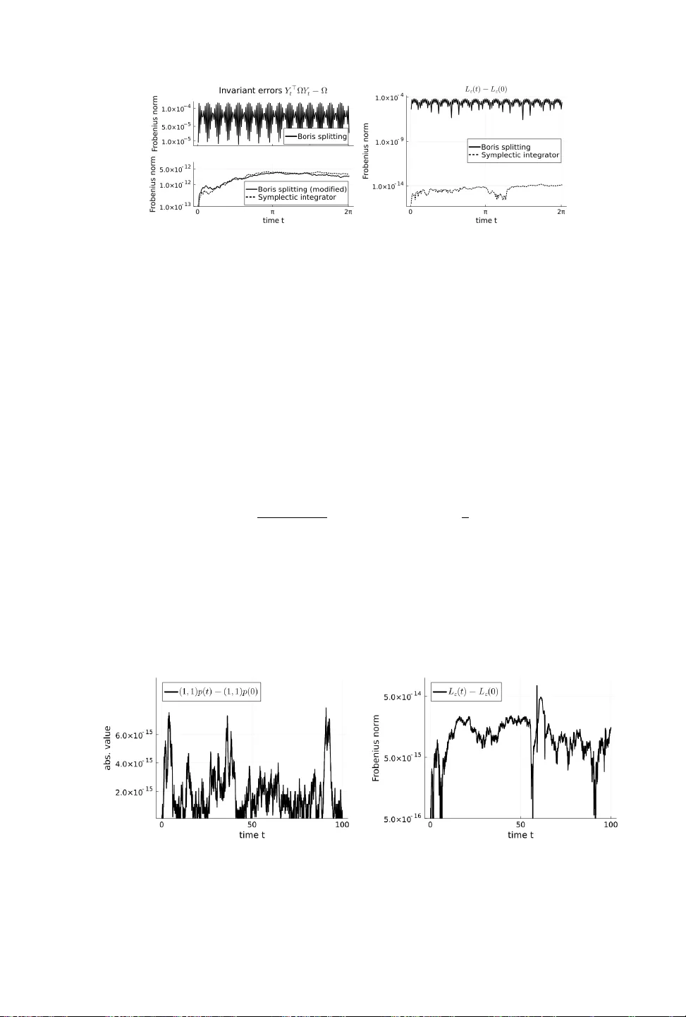
Original Paper
Loading high-quality paper...
Comments & Academic Discussion
Loading comments...
Leave a Comment