Topological optimization with birth and death cochains

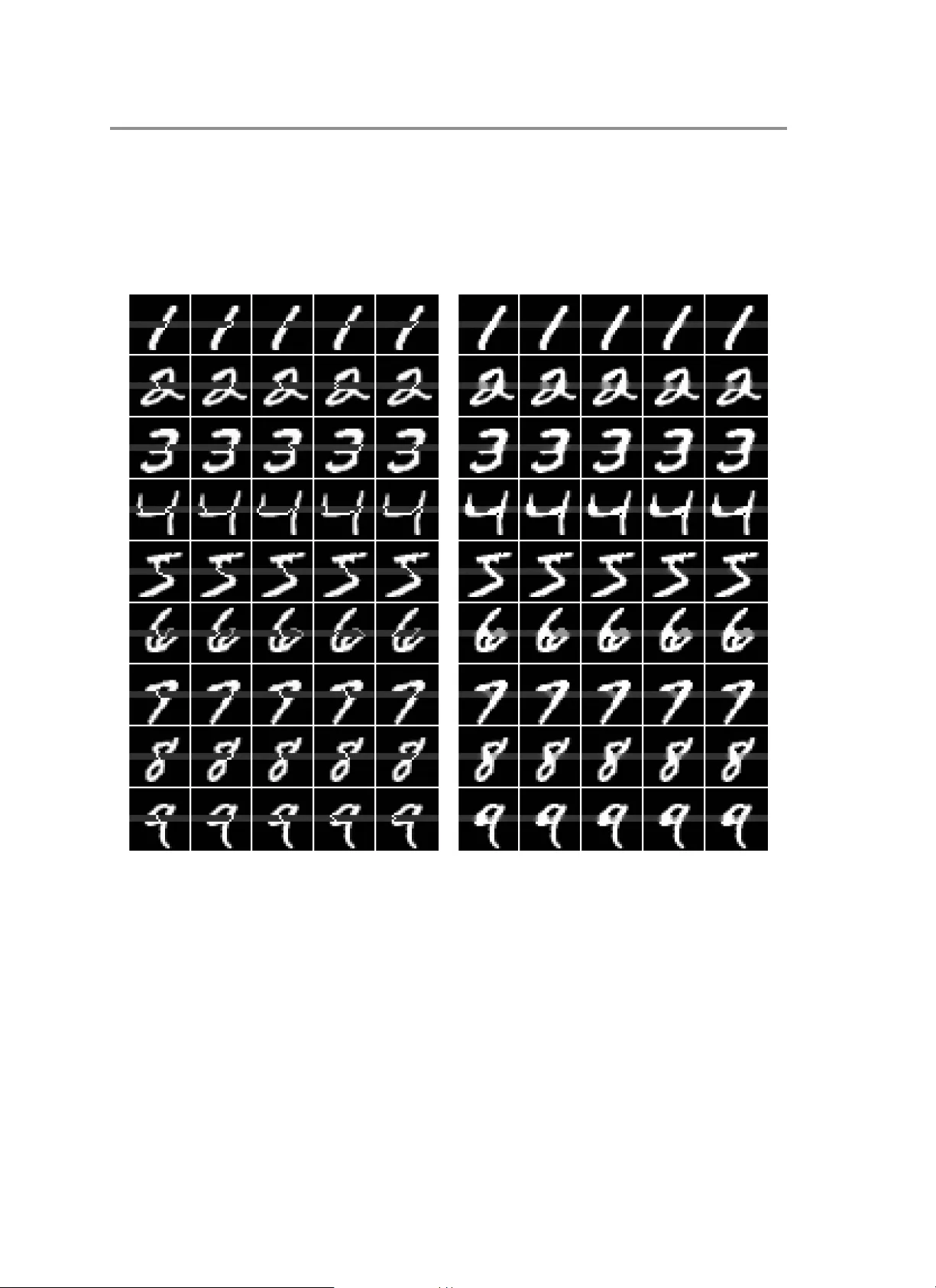
T op ological optimization with birth and death co chains ∗ Thomas W eighill † and Ling Zhou ‡ Abstract. W e in troduce the notion of birth and death co c hains as generalized versions of birth and death simplices in p ersisten t cohomology . W e sho w that birth and death cochains (unlik e birth and death simplices) are alw ays unique for a giv en persistent cohomology class. W e use birth and death co c hains to deﬁne birth and death con ten t as generalizations of birth and death times. W e then demonstrate the adv an tages of using that birth and death conten t as loss functions on a v ariety of topological optimization tasks with p oint clouds, time series and scalar ﬁelds. W e close with a nov el application of top ological optimization to a dataset of arctic ice images. Key w o rds. p ersistence diagram, p ersisten t cohomology , top ological optimization, gradient descen t MSC co des. 55N31, 68T09 1. Intro duction. P ersisten t homology and cohomology quan tify the shape of data b y trac king the top ology of a datset at v arious thresholds (or scales) [ 13 , 28 , 12 , 6 , 10 ]. A top ological feature suc h as a connected comp onent or hole is “born” at one threshold and “dies” at later threshold. The time b etw een these tw o even ts is the p ersistence of the feature, and this v alue often quan tiﬁes its importance in the ov erall structure of the data. Birth and death times are recorded as pairs [ b, d ) to create a p ersistence diagram, whic h is known to b e stable with resp ect to p erturbations in the underlying data [ 8 ]. The birth–death pair [ b, d ) records only partial information ab out a top ological feature: it sp eciﬁes the parameter v alues at whic h the feature app ears and disapp ears, but not the sp eciﬁc c hanges in the underlying ﬁltered spaces resp onsible for these even ts. In practice, these ev en ts are realized b y particular simplices in the ﬁltration. W e refer to the simplex whose addition creates (resp. destro ys) a feature as its birth simplex (resp. de ath simplex ); see Figure 1 for a to y example. These birth and death simplices, despite b eing absent from a p ersistence diagram, are imp ortant in many applications. F or example, they can b e used to localize or visualize top ological features in the underlying data [ 11 , 16 ], and they pla y an imp ortan t role in several optimization frameworks inv olving p ersisten t (co)homology [ 7 , 5 ]. Despite their utilit y , birth and death simplices hav e some notable drawbac ks: (a) they are highly lo calized: mo difying a birth or death simplex amounts to changing only a small p ortion of the data, (b) they can fail to be well-deﬁned (if tw o simplices share a ﬁltration v alue), and (c) they can b e highly unstable: birth and death simplices can b e altered by small p er- turbations in the data (unlik e birth and death times). F or example, in the p oint cloud example in Figure 1 , trying to decrease the birth time of the ∗ F unding: L.Z. received supp ort from an AMS–Simons T ravel Grant. † Depa rtment of Mathematics and Statistics, Universit y of North Ca rolina at Greensb oro, Greensb o ro, NC ( t weighill@uncg.edu ). ‡ Depa rtment of Mathematics, Duke University , Durham, NC ( ling.zhou@duk e.edu ). 1 2 T. WEIGHILL AND L. ZHOU Figure 1: The classical notion of birth simplex (in green) and death simplex (purple) for degree-1 p ersisten t homology . hole by focusing on the birth edge alone amoun ts to changing just t w o p oints. Moreov er, a tin y disturbance of the p oint could c hange the lo cation of the green edge while still preserving the same “hole”. In this pap er, we attempt to address these shortcomings b y relaxing the notion of birth and death simplices. W e introduce birth and de ath c o chains , whic h are linear combinations of (dual) simplices relev ant to the birth and death of a feature resp ectiv ely . In the most general deﬁnition, birth and death co chains are deﬁned for a simplicial pair K ⊆ L as the solution to  2 optimization problems which generalize those related to harmonic co c hains. Among our theoretical results, w e prov e the uniqueness of these ob jects, and relate them to relative cohomology , Laplace learning, and p ersistent Laplacians ( Section 3 ). When dealing with p ersisten t cohomology , K and L b ecome snapshots of the ﬁltration just b efore and after birth or death (see Figure 2 ), giving rise to ε -birth and ε -de ath c o chains . Dra wbac ks (a) and (b) listed ab o v e are av oided by ε -birth and ε -death co c hains since they in v olv e m ultiple simplices at once, and are alwa ys unique (see Theorem 3.4 ) and well-deﬁned for a giv en persistent cohomology class. While w e ha v e goo d reason not to expect a theoretical guaran tee of stabilit y for ε -birth and ε -death co chains, we ha v e a heuristic argument for wh y they may b e more stable than birth and death simplices in practice (see Section 6 ). Our hypothesis is supp orted by b etter conv ergence to regular conﬁgurations for p oint-clouds ( Section 7 ), and more robust behavior on low er-star ﬁltrations ( Section 8 ). b − ε b + ε d − ε d + ε birth–death pair [ b, d ) ε -birth co chain ε -death co chain Figure 2: The ε -birth cochain which lives at b − ε is computed for a co chain at b + ε , and the ε -death co c hain whic h lives at d + ε is computed for a co chain at d − ε . See Subsection 3.2 . W e use ε -birth and ε -death co c hains to introduce a relaxation of the notion of birth time and death time, which w e call ε -birth c ontent and ε -de ath c ontent resp ectiv ely . These quan tities appro ximate classical birth and death times for small ε , but dep end on m ultiple simplices, making them perform b etter as ob jectiv e functions in top ological optimization BIRTH AND DEA TH COCHAINS 3 Figure 3: Optimizing a point cloud using birth and death cochains (see Section 7 ). W e plot the ob jectiv e function to b e maximized, along with snapshots of the p oin ts cloud every 100 iterations. The birth cochain is sho wn using green edges and the death cochain is sho wn using purple triangles; these are the simplices that are adjusted in the gradient ascent step. tasks. Figure 3 sho ws a visualization of top ological optimization on p oint clouds using birth and death cochains; note ho w m ultiple simplices are in v olv ed at eac h gradien t ascent step. W e pro v e that regular p olygons are critical p oints of Vietoris-Rips ε -p ersistence con ten t (i.e. ε - death con ten t min us ε -birth conten t) under suitable constraints ( Theorem 5.6 ). By contrast, birth and death simplices are not ev en w ell-deﬁned for regular polygons, and are v ery unstable for almost-regular conﬁgurations. While birth and death co chains can b e useful in an y application in v olving birth and death simplices, our fo cus in this pap er is on topological optimization, where a top ological loss function is minimized either as a standalone ob jective or as part of a regularizer. T o demonstrate the adv an tages of birth and death co chains, w e deploy them in three model optimization tasks: • On p oin t clouds, we show that using co chains instead of simplices often gives b et- ter long-term con v ergence and av oids loc al optima, leading to improv ed normalized p ersistence ( Section 7 ). • On image data, optimization using cochains av oids arbitrary choices and results in smo other, more realistic solutions ( Section 8 ). • F or feature selection, w e ﬁnd that ev en a naiv e line-searc h metho d eﬀectiv ely ﬁnds features relev ant to a top ological feature when using co c hains ( Section 9 ). W e conclude our demonstration of cochains in top ological optimization with a nov el ap- plication to Arctic ice extent data ( Section 10 ). W e deplo y the naiv e line-search metho d for feature selection on satellite images of ice, revealing the sp eciﬁc assymetry in the melting and freezing cycle that causes the “hole” in the data observ ed by p ersistent homology , conﬁrming the h yp othesis in [ 17 ]. 2. Prelimina ries. Throughout this pap er, all simplicial complexes are ﬁnite. In this sec- tion w e ﬁx notation and recall the basic notions from simplicial cohomology and p ersisten t 4 T. WEIGHILL AND L. ZHOU cohomology that will b e used throughout. 2.1. Cohomology and Harmonic Rep resentatives. All (co)homology groups are taken with co eﬃcien ts in R . F or a simplicial complex X and a degree k , the space of k -co chains C k ( X ) consists of all real-v alued functions on the set X k of k -simplices of X . W e equip C k ( X ) with the standard  2 inner pro duct deﬁned by ⟨ α, β ⟩ := X σ ∈ X k α ( σ ) β ( σ ) , α, β ∈ C k ( X ) , and denote the induced norm b y ∥ α ∥ 2 . W e denote by δ k : C k ( X ) → C k +1 ( X ) the k -th cob oundary op erator and b y ( δ k ) ∗ its adjoin t with resp ect to the  2 inner pro duct. More generally , w e use ( · ) ∗ to denote the adjoint of a linear op erator b et w een ﬁnite-dimensional inner pro duct spaces. A k -co chain α is called a c o cycle if δ k α = 0, and a c ob oundary if α ∈ im δ k − 1 . W e denote the spaces of k -co cycles and k -cob oundaries by Z k ( X ) := ker δ k and B k ( X ) := im δ k − 1 , respectively . The k -th c ohomolo gy gr oup is deﬁned as H k ( X ) := Z k ( X )  B k ( X ) . F or a co cycle α , we write [ α ] to denote its cohomology class. Giv en a cohomology class [ α ] ∈ H k ( X ), its harmonic r epr esentative is the unique co cycle ˆ α in the class [ α ] that minimizes the  2 norm. In other w ords, it is the unique elemen t in arg min n ∥ α ′ ∥ 2    α ′ ∈ C k ( X ) , α ′ ∈ [ α ] o . Equiv alently , it is the unique co c hain ˆ α ∈ [ α ] satisfying ∆ k ˆ α = 0 , where ∆ k := ( δ k ) ∗ δ k + δ k − 1 ( δ k − 1 ) ∗ denotes the k -th com binatorial Hodge Laplacian. 2.2. P ersistent Cohomology . A ﬁltr ation of top ological spaces is a collection { X t } t ∈ R suc h that X t ⊆ X s whenev er t ≤ s . In this pap er, w e focus on ﬁltrations of ﬁnite simplicial complexes, whic h can b e represented as a ﬁnite nested sequence of sub complexes: X t 0 ⊆ X t 1 ⊆ · · · ⊆ X t n = X . That is, there exist t 0 < t 1 < · · · < t n suc h that X t = X t i for all t ∈ [ t i , t i +1 ). W e primarily consider ﬁltrations of the following types: • The sublevel-set ﬁltr ations , deﬁned as { X t } t ∈ R with X t = { σ ∈ X | f ( σ ) ≤ t } for a simplicial complex X and a real-v alued function f on the simplices of X . • The lower star ﬁltr ation , { Lo wSt( K, t ) } t ∈ R , for a simplicial complex K with v ertex set V and f : V → R , where Lo wSt( K, t ) consists of simplices whose v ertices hav e function v alue at most t . • The Vietoris–Rips ﬁltr ations , deﬁned as { VR( M ; t ) } t ∈ R for a metric space ( M , d ), where VR( M ; t ) consists of all ﬁnite subsets σ ⊆ M with max x,y ∈ σ d ( x, y ) ≤ t . Equiv a- len tly , this is the sublev el-set ﬁltration of the diameter function f ( σ ) = max x,y ∈ σ d ( x, y ) on the full simplex o v er M . Throughout this pap er, w e w ork with cohomology rather than homology . While b oth theories pro vide the same information for ﬁnite simplicial complexes o v er a ﬁeld (b y the univ ersal co eﬃcient theorem), cohomology is more conv enien t for our purp oses, especially when w orking with harmonic represen tativ es and optimization problems. BIRTH AND DEA TH COCHAINS 5 Giv en a ﬁltration { X t } t ∈ R , the k -th cohomology groups H k ( X t ) assemble in to a p ersistence mo dule, with structure maps induced by the inclusions X t  → X s for t ≤ s : H k ( X t 0 ) ← H k ( X t 1 ) ← · · · ← H k ( X t n ) . This p ersistence module is referred to as the k -th p ersistent c ohomolo gy of the ﬁltration. By the structure theorem for p ersistence mo dules (see, e.g., [ 9 , 23 ]), the k -th p ersisten t cohomology decomp oses as a direct sum of interv al mo dules (i.e., p ersistence mo dules sup- p orted on a single interv al). This decomp osition is enco ded b y a multiset of interv als, called the b ar c o de (or p ersistence diagram) in degree k . W e adopt the con v en tion that persistence in terv als, also called b ars , are half-op en of the form [ b, d ), so that a class exists for b ≤ t < d and disapp ears at t = d . F or each bar [ b i , d i ), we refer to b i and d i as its birth and de ath times. 2.3. Relative Cohomology . F or clarit y , when necessary , w e add the underlying space as a subscript to the cob oundary operator and cohomology class, e.g., δ k X and [ · ] X , to indicate that the cob oundary or cohomology class is taken with resp ect to the complex X . Consider a sub complex K of a complex L . The r elative c o chain gr oup C k ( L, K ) consists of k -co c hains on L that v anish when restricted to K ; that is, C k ( L, K ) := n ϕ L ∈ C k ( L )    ϕ L | K = 0 o , where ϕ L | K ∈ C k ( K ) denotes the restriction of ϕ L to the k -simplices of K . These groups assem ble in to the r elative c o chain c omplex · · · → C k − 1 ( L, K ) δ k − 1 − − − → C k ( L, K ) δ k − → C k +1 ( L, K ) → · · · , where the coboundary maps are induced from those on L . The relativ e cohomology groups H k ( L, K ) are deﬁned as the cohomology of this complex. The standard inner pro duct on C k ( L ) restricts to an inner product on C k ( L, K ). Let ι : K  → L b e the inclusion of simplicial complexes. The r estriction map ι # : C k ( L ) → C k ( K ) sends a co c hain φ ∈ C k ( L ) to its restriction on the k -simplices of K . The extension by zer o map  : C k ( K )  → C k ( L ) em b eds a co c hain on K into L b y assigning zero to all k -simplices in L \ K . By standard abuse of notation, we also write ι # : H k ( L ) → H k ( K ) for the induced map on cohomology . With resp ect to the standard inner pro duct on co chains, the subspaces C k ( L, K ) and  (C k ( K )) are orthogonal complemen ts in C k ( L ). Accordingly , we ha v e the orthogonal decomp osition (2.1) C k ( L ) = C k ( L, K ) ⊥ ⊕ C k ( L, K ) , C k ( L, K ) ⊥ =  (C k ( K )) . 3. Birth and death co chains. 3.1. Birth and death co chains fo r simplicial pairs. Let K b e a sub complex of the sim- plicial complex L . W e study the change in simplicial cohomology from K to L . There are t w o primary scenarios, informally describ ed as: • (Birth) A cohomology class whic h does not exist at K app ears at L , and • (Death) A cohomology class whic h exists at K “dies” (i.e. is no longer present) in L . 6 T. WEIGHILL AND L. ZHOU More formally , we hav e the following deﬁnitions. Deﬁnition 3.1. L et K b e a sub c omplex of the simplicial c omplex L . We say a c ohomolo gy class [ α ] L ∈ H k ( L ) is b orn betw een K and L if [ α | K ] = 0 ∈ H k ( K ) . We say that a c ohomolo gy class [ β ] K ∈ H k ( K ) dies b etw een K and L if β c annot b e extende d to a k -c o cycle on L . Supp ose [ α ] L ∈ H k ( L ) is born b etw een K and L . W e b egin b y noting that there is a rep- resen tativ e ˆ α ∈ [ α ] L whose restriction to K is the zero co c hain (not just zero in cohomology). Indeed, α | K is a cob oundary in K , so α | K = δ k K f for some f ∈ C k − 1 ( K ). Extending f by zero, w e note that α − δ k L f is cohomologous to α and restricts to zero on K as required. Deﬁnition 3.2 (Birth co chain). L et K ⊆ L and let [ α ] L ∈ H k ( L ) b e b orn b etwe en K and L . The birth co c hain for α from K to L is the unique element ˆ α of arg min α ′ ∈ C k ( L )  || α ′ || 2   α ′ | K = 0 , α ′ ∈ [ α ] L  . Uniqueness of ˆ α is addressed in Theorem 3.4 b elo w. Figure 4 illustrates a simple example of a birth co c hain. In the sp ecial case of K = ∅ , the condition ˆ α | K = 0 is v acuous, and the birth co c hain reduces to the  2 -minimal (harmonic) represen tativ e of [ α ] L . Th us, birth co c hains generalize harmonic representativ es to the setting of simplicial pairs. A t the opposite extreme, if K = L , no nontrivial class can b e b orn betw een K and L . W e no w consider death, which happens when there is an [ β ] K ∈ H k ( K ) which cannot b e extended to a co cycle in H k ( L ). Deﬁnition 3.3 (Death cochain). L et K ⊆ L and let [ β ] K ∈ H k ( K ) die b etwe en K and L . The death co chain for β from K to L is δ k L ˆ β , wher e ˆ β is any element in (3.1) arg min β ′ ∈ C k ( L ) n ∥ δ k L β ′ ∥ 2    β ′ | K = β o . A ny such ˆ β is c al le d a death potential . Figure 5 shows a simple example of a death co chain. In Prop osition 4.2 , we will in- terpret the death co chain as the  2 -minimal represen tativ e of the relative cohomology class [ δ k L  ( β )] ( L,K ) , where  denotes the extension-by-zero map and the subscript ( L, K ) indicates that the cohomology class is taken in H k +1 ( L, K ). In the sp ecial case when L and K hav e the same k -sk eleton (e.g. L = K ), the death p oten tial can only b e β itself. While the birth co c hain clearly do es not depend on the c hoice of the represen tativ e α , the same is not immediately clear for the death co chain. While a direct pro of is p ossible, the fact that the death co c hain is indep enden t of the c hoice of representativ e will actually follow from the formulation of birth and death co c hains in terms of relativ e cohomology in the next section; see Corollary 4.3 . F or now we note that with this in mind: we can reformulate the optimization problem in Deﬁnition 3.3 as arg min ω ∈ C k +1 ( L ) n || ω || 2    ω = δ k L β ′ , β ′ | K ∈ [ β ] K o . R emark 3.4 (Uniqueness of birth and death co chains). The minimizers in Deﬁnitions 3.2 and 3.3 are unique. In eac h case the feasible set is an aﬃne subset of a ﬁnite-dimensional BIRTH AND DEA TH COCHAINS 7 co c hain space deﬁned b y linear constrain ts, and the squared  2 norm is strictly conv ex. Hence the minimizer is uniquely determined. (a) K (b) L and α ∈ C 1 ( L ) (c) birth co c hain Figure 4: The birth co chain for the cohomology class α b orn b et w een K and L , where the edge v alues show the co eﬃcients in each 1-chain. (a) K and β ∈ C 1 ( K ) (b) L (c) death co c hain Figure 5: The death co chain for the cohomology class β whic h dies b et w een K and L . W e sho w the coeﬃcients of the death co chain on each 2-s implex in white and the co eﬃcien ts of the death p oten tial on each edge in black. R emark 3.5 (Homogeneity of birth and death co chains). Since p ersisten t cohomology classes are typically only deﬁned up to scalar multiplication, it is worth while observing the eﬀects of scalar multiplication on birth and death co chains. In each of the optimization prob- lems, m ultiplying the p ersistent cohomology class by a scalar multiplies the feasible regions b y the same scalar. Since the ob jectiv e function in each case is absolutely homogeneous, it follo ws that the birth and death cochains are also scaled by the same amount. 3.2. Birth and death co chains in p ersistence mo dules. W e now place the preceding construction in the setting of p ersisten t cohomology . Let { X t } t ∈ R b e a ﬁltration of simplicial complexes and ﬁx a bar [ b, d ) in degree k . Asso ciated to the interv al mo dule for this bar is a family of non-zero cohomology classes deﬁned up to scalar multiplication { c t ∈ H k ( X t ) } t ∈ [ b,d ) suc h that whenever b ≤ s < t < d , the class c t maps to c s under the homomorphism induced b y the inclusion X s ⊆ X t . W e will refer to the collection of the c t as a p ersistent c ohomolo gy 8 T. WEIGHILL AND L. ZHOU class for the bar [ b, d ). Birth and death ev en ts o ccur at the transition pairs X b − ε ⊆ X b + ε and X d − ε ⊆ X d + ε , for suﬃciently small ε > 0. Applying the deﬁnitions of Deﬁnitions 3.2 and 3.3 to these pairs yields the follo wing. Deﬁnition 3.6 ( ε -birth and death co chains). L et c b e the p ersistent c ohomolo gy class for a b ar [ b, d ) and let 0 < ε < d − b . The ε -birth co c hain for c is the birth c o chain of c b + ε fr om X b − ε to X b + ε . The ε -death co c hain for c is the de ath c o chain of c d − ε fr om X d − ε to X d + ε . See Figure 2 for a schematic visualization of the construction in Deﬁnition 3.6 . W e remark that it is possible to c hoose a diﬀerent ε for eac h of the four occurrences in Deﬁnition 3.6 ab o v e, but in practice it is con v enien t to ha v e one parameter. R emark 3.7. Let X t 0 ⊆ X t 1 ⊆ · · · ⊆ X be a ﬁltration suc h that X t i and X t i +1 diﬀer by a single simplex for each i . If ε < min i { t i +1 − t i } , then the ε -birth co c hain for a bar [ b, d ) has supp ort equal to the unique simplex in X b + ε \ X b . Similarly , any ε -death co chain has supp ort equal to single simplex. In other words, for small ε , the birth and death cochains are dual to birth and death simplices resp ectiv ely . W e ha v e th us deﬁned a generalization of birth and death simplices as promised. 4. Interp retations of birth and death co chains. In this section w e rein terpret birth and death co c hains from several complemen tary persp ectives. 4.1. Birth and death co chains via relative cohomology . W e giv e an alternativ e c harac- terization of birth and death co c hains using relativ e cohomology . Throughout, let K ⊂ L b e simplicial complexes. Recall from Subsection 2.3 that the relativ e co c hain group C k ( L, K ) consists of k –co c hains on L that v anish on K , and that the relativ e cohomology group H k ( L, K ) is deﬁned as the cohomology of this complex. The inclusion ι : K  → L induces the long exact sequence [ 15 ] (4.1) · · · / / H k ( L, K ) q # / / H k ( L ) ι # / / H k ( K ) λ # / / H k +1 ( L, K ) / / · · · . Here q # is induced b y the inclusion of relative co chains into absolute co c hains, ι # is induced b y restriction to K , and λ # is the connecting homomorphism, deﬁned b y (4.2) λ # ([ β ] K ) := [ δ k L β ′ ] ( L,K ) , where β ′ ∈ C k ( L ) is an y extension of β to L . In particular, one ma y tak e β ′ to be the extension of β by zero outside K . The connecting homomorphism is w ell-deﬁned: if β ′ extends β , then ( δ k L β ′ ) | K = δ k K β = 0 since β is a co cycle on K , so δ k L β ′ ∈ C k +1 ( L, K ). The prop osition b elo w on birth co chains is motiv ated by the follo wing observ ation. If [ α ] L is b orn b et w een K and L , then ι # ([ α ] L ) = 0 ∈ H k ( K ), so b y the exactness of ( 4.1 ), [ α ] L is the image of q # . Prop osition 4.1. The birth c o chain for [ α ] L fr om K to L is the unique element of arg min α ′ ∈ Z k ( L,K ) n ∥ α ′ ∥ 2    q # ([ α ′ ] ( L,K ) ) = [ α ] L o . BIRTH AND DEA TH COCHAINS 9 Pr o of. Comparing with Deﬁnition 3.2 , w e see that α ′ ∈ Z k ( L, K ) is precisely the condition that α ′ | K = 0, and q # ([ α ′ ] ( L,K ) ) = [ α ] L is precisely the condition that α ′ represen ts [ α ] as an elemen t of H k ( L ). The prop osition b elow on death co chains is motiv ated by the follo wing observ ation. Since [ β ] K cannot b e extended to a co cycle on L , it is not in the image of ι # . By the exactness of ( 4.1 ), the cohomology class λ # ([ β ] K ) is nonzero. Prop osition 4.2. The de ath c o chain for [ β ] K fr om K to L is the unique element of arg min ω ∈ Z k +1 ( L,K ) n ∥ ω ∥ 2    [ ω ] ( L,K ) = λ # ([ β ] K ) o . Pr o of. It suﬃces to sho w that the following e qualit y of sets holds: (4.3) n ω    ω = δ k L β ′ for β ′ ∈ C k ( L ) , β ′ | K = β o = n ω ∈ Z k +1 ( L, K )    [ ω ] ( L,K ) = λ # ([ β ] K ) o . Supp ose ω = δ k L β ′ for some β ′ ∈ C k ( L ) with β ′ | K = β . Since ω is a cob oundary in L , it is a co cycle in L . Moreo v er, since the restriction of β ′ to K equals β , and β is a co cycle on K , it follo ws that ω | K = δ k K ( β ′ | K ) = δ k K β = 0. Thus ω v anishes on K , so ω ∈ Z k +1 ( L, K ). Since β ′ extends β , the deﬁnition of the connecting homomorphism gives [ ω ] ( L,K ) = [ δ k L β ′ ] ( L,K ) = λ # ([ β ] K ) . Hence the inclusion ‘ ⊆ ’ in ( 4.3 ) holds. Con v ersely , supp ose ω ∈ Z k +1 ( L, K ) satisﬁes [ ω ] ( L,K ) = λ # ([ β ] K ). Let β 1 ∈ C k ( L ) b e an y extension of β , so β 1 | K = β . By deﬁnition of the connecting homomorphism, ω − δ k L β 1 ∈ B k +1 ( L, K ) . Thus there exists β 2 ∈ C k ( L, K ) suc h that ω − δ k L β 1 = δ k L β 2 . Setting β ′ = β 1 + β 2 , w e obtain ω = δ k L β ′ . Moreov er, since β 2 v anishes on K , β ′ | K = β 1 | K + β 2 | K = β + 0 = β . Hence ω lies in the left-hand set of ( 4.3 ), which prov es the inclusion ‘ ⊇ ’. Co rolla ry 4.3. Supp ose [ β ] K dies b etwe en K and L . Then the de ath c o chain do es not dep end on the r epr esentative for [ β ] K . 4.2. Birth co chains in degree 0 . Birth cochains admit a particularly simple description in degree 0, where cohomology classes hav e canonical represen tativ es. The situation for death co c hains in degree 0 turns out to b e equiv alen t to so-called Laplace learning on graphs (see Subsection 4.3 ). Since degree-0 cohomology dep ends only on the 1-skeleton of the ﬁltration, it suﬃces to w ork with graphs. Throughout this subsection, let G = ( V , E ) b e a ﬁnite graph with vertex set V and edge set E , equipp ed with a function f : V → R inducing a sublevel-set ﬁltration. W e assume for simplicity that f is injective; if not, then certain non-canonical c hoices might need to b e made to deﬁne persistent cohomology classes (say by ﬁxing an ordering of the v ertices). F or any t ∈ R , write G t := f − 1 (( −∞ , t ]) for the sublev el set at t , and let V t denote its v ertex set. It is easy to see that 0-co cycles for G t are functions V t → R whic h are constant on connected comp onen ts, and that each cocycle is the unique represen tativ e for a cohomology class. F or an y vertex v ∈ V t , denote by G v t ⊂ G t the connected comp onent containing v , and b y V v t the v ertex set of G v t . 10 T. WEIGHILL AND L. ZHOU Let [ b, d ) b e a ﬁnite bar in the 0-dimensional p ersistence barco de for the ﬁltration { G t } t ∈ R and let v b e the vertex with f ( v ) = b . Let d − = max { t ∈ Im f | t < d } . Then a p ersisten t cohomology class for this bar is giv en by { [ α t ] } t ∈ [ b,d ) where α t ( u ) = ( 1 u ∈ V v d − ∩ G t 0 otherwise Indeed, the fact that a birth ev en t tak es place at b implies that α b has supp ort { v } , and the rest is determined by the fact that α t is constan t on connected comp onents. Since cohomology classes ha v e unique represen tativ es, the ε -birth co c hain is just α b + ε , that is, the indicator function on all vertices whic h will b e connected to v b efore the death time d and whose ﬁltration v alues are at most b + ε . 4.3. Death cochain via Laplace lea rning. Laplace learning is a classical metho d in semi- sup ervised learning that constructs a function on a graph by minimizing Dirichlet energy sub ject to ﬁxed b oundary v alues [ 27 ]. Let L b e a ﬁnite simplicial complex of dimension 1, i.e., a graph, and K a sub complex of L . Let ∆ 0 , up L := ( δ 0 L ) ∗ δ 0 L denote the (com binatorial) graph Laplacian. Giv en v ertex lab els g : K 0 → R , Laplace learning solv es arg min f ∈ C 0 ( L )  ∥ δ 0 L f ∥ 2 2   f | K = g  . Equiv alently , the solutions f are c haracterized b y the follo wing conditions [ 27 , Section 2]: (4.4) f | K = g and (∆ 0 , up L f )   L \ K = 0 . Let K ⊆ L b e simplicial complexes and [ β ] K ∈ H k ( K ) die b et w een K and L . Recall from Deﬁnition 3.3 that the death cochain of [ β ] K is deﬁned as δ k L ˆ β , where ˆ β is a death potential that solv es the optimization problem arg min β ′ ∈ C k ( L ) n ∥ δ k L β ′ ∥ 2    β ′ | K = β o . Th us, death co c hains ma y b e view ed as higher-order generalizations of Laplace learning. In the graph setting, one prescrib es arbitrary v alues on K , whereas here the prescrib ed co chain β is required to b e a co cycle, since it represents a cohomology class that b ecomes trivial in L . One could just as easily formulate the same v ariational problem ( Equation (3.1) ) for an arbitrary cochain β on K ; how ev er, without the co cycle condition some of the top ological in terpretations (suc h as the relativ e cohomology viewpoint) w ould b e lost. By analogy with the graph case (see Equation (4.4) ), the death co chain problem can b e view ed as a higher–order Dirichlet problem. In particular, the minimizer satisﬁes a relativ e harmonicit y condition analogous to Laplace learning. W e state this precisely in Proposition 4.4 and include a brief proof for completeness. Let ∆ k, up L := ( δ k L ) ∗ δ k L : C k ( L ) → C k ( L ) denote the k -th up Laplacian on L . BIRTH AND DEA TH COCHAINS 11 Prop osition 4.4. L et [ β ] K ∈ H k ( K ) die b etwe en K and L . The de ath p otentials ˆ β ar e char acterize d by the fol lowing c onditions: ˆ β | K = β and (∆ k, up L ˆ β )   L \ K = 0 . Pr o of. Let  : C k ( K ) → C k ( L ) denote the extension-by-zero map, and write ˆ β =  ( β ) + γ with γ ∈ C k ( L, K ), with resp ect to the decomp osition in ( 2.1 ). Then the ob jectiv e function in the death co c hain problem b ecomes a quadratic polynomial in γ . At a minim um, its gradient with resp ect to γ must v anish in all admissible directions η ∈ C k ( L, K ), i.e. d dt    t =0 ∥ δ k L ( ˆ β + tη ) ∥ 2 2 = d dt    t =0  ∥ δ k L ˆ β ∥ 2 2 + 2 t ⟨ ∆ k, up L ˆ β , η ⟩ + t 2 ∥ δ k L η ∥ 2 2  = 2 ⟨ ∆ k, up L ˆ β , η ⟩ = 0 . Th us ∆ k, up L ˆ β is orthogonal to C k ( L, K ), which is equiv alen t to (∆ k, up L ˆ β ) | L \ K = 0 . 4.4. Death co chain via p ersistent Laplacian. The p ersisten t Laplacian extends the com- binatorial Laplacian to pairs of simplicial complexes [ 19 , 26 , 22 ]. In the c hain-complex (i.e. ho- mology) setting, a c haracterization of the p ersistent Laplacian in terms of Sch ur complements w as established in [ 22 ]. The corresp onding formulation in the co c hain setting was developed in [ 14 ]. W e brieﬂy recall the relev an t constructions. Let ∆ : V → V be a self-adjoint p ositiv e semideﬁnite op erator on a ﬁnite-dimensional inner pro duct space, and let V = W ⊕ W ⊥ b e an orthogonal decomp osition. With resp ect to this decomp osition (and an y choice of bases adapted to it), the op erator ∆ admits a blo c k matrix represen tation (4.5) ∆ =  ∆ W W ∆ W ⊥ ∆ ⊥ W ∆ ⊥⊥  . The (gener alize d) Schur c omplement of ∆ ⊥⊥ in ∆ is deﬁned as ∆ W W − ∆ W ⊥ ∆ + ⊥⊥ ∆ ⊥ W , where ( · ) + denotes the Mo ore–Penrose pseudoinv erse. As noted in [ 14 , Proposition 9], view ed as a linear op erator, the Sc h ur complement is independent of the choice of bases and therefore is canonically determined by the pair (∆ , W ). This op erator is called the Schur r estriction of ∆ on to W and denoted as Sc h(∆ , W ) : W → W. As b efore, let  : C k ( K )  → C k ( L ) b e the extension by zero map. Deﬁne the subspace C k +1 L,K := n ξ ∈ C k +1 ( L )    ( δ k L ) ∗ ( ξ ) ∈  (ker(( δ k − 1 K ) ∗ )) o ⊂ C k +1 ( L ) , and let ∂ L,K k +1 denote the restriction of ( δ k L ) ∗ to C k +1 L,K . The de gr e e- k p ersistent up L aplacian is ∆ k, up L,K := ∂ L,K k +1 ◦ ( ∂ L,K k +1 ) ∗ : C k ( L, K ) ⊥ → C k ( L, K ) ⊥ =  (C k ( K )) . R emark 4.5. Let W :=   k er(( δ k − 1 K ) ∗ )  ⊆  (C k ( K )). It follo ws from [ 14 , Prop osition 10] that the Sc h ur restriction of δ k L on to W and the degree- k persistent up Laplacian satisﬁes ∆ k, up L,K = ι W ◦ Sc h( δ k L , W ) ◦ pro j W , where pro j W :  (C k ( K )) → W is the orthogonal pro jection and ι W : W  →  (C k ( K )) is the inclusion. W e give a detailed explanation of the ab ov e equality in Section A . 12 T. WEIGHILL AND L. ZHOU Theo rem 4.6. L et K ⊂ L b e simplicial c omplexes and let [ β ] K ∈ H k ( K ) die b etwe en K and L . Then, the squar e d norm of the de ath c o chain δ k L ˆ β satisﬁes (4.6) ∥ δ k L ˆ β ∥ 2 2 = D Sc h  ∆ k, up L ,  (C k ( K ))   ( β ) ,  ( β ) E . When β is harmonic on K , we have (4.7) ∥ δ k L ˆ β ∥ 2 2 = D ∆ k, up L,K (  ( β )) ,  ( β ) E . Pr o of. Let U :=  (C k ( K )) and U ⊥ b e its orthogonal complemen t in C k ( L ). Then, an y death p otential ˆ β can be written as ˆ β =  ( β ) + γ with γ ∈ U ⊥ . With respect to the decom- p osition C k ( L ) = U ⊕ U ⊥ (and any c hoice of bases adapted to it), write the blo ck matrix represen tation of ∆ k, up L as in (4.5) . Then the ob jectiv e function of the death co c hain problem is the quadratic form of the positive semideﬁnite op erator ∆ k, up L = ( δ k L ) ∗ δ k L , satisfying ∥ δ k L ˆ β ∥ 2 2 = ⟨ ∆ k, up L (  ( β ) + γ ) ,  ( β ) + γ ⟩ = ⟨ ∆ U U  ( β ) ,  ( β ) ⟩ + 2 ⟨ ∆ U ⊥ γ ,  ( β ) ⟩ + ⟨ ∆ ⊥⊥ γ , γ ⟩ . (4.8) W e no w inv ok e a standard quadratic minimization result [ 4 , Example 3.15]: if f ( x, y ) = x T Ax + 2 x T B y + y T C y is p ositiv e semideﬁnite with A and C symmetric, then inf y f ( x, y ) = x T ( A − B C † B T ) x. Applying this with x =  ( β ), y = γ , A = ∆ U U , B = ∆ U ⊥ , C = ∆ ⊥⊥ , and the deﬁnition of Sc h ur restriction, w e obtain (4.6) . If β is harmonic on K , then β ∈ ker( δ k K ) ∩ ker(( δ k − 1 K ) ∗ ) , implying that  ( β ) ∈ W :=   k er(( δ k − 1 K ) ∗ )  . Via a similar argumen t as ab o v e, by replacing U with W , we obtain ∥ δ k L ˆ β ∥ 2 2 = D Sc h  ∆ k, up L , W   ( β ) ,  ( β ) E . Finally , using the relationship betw een the Sc h ur restriction and the persistent Laplacian from Theorem 4.5 , along with  ( β ) ∈ W and ι W = (pro j W ) ∗ , w e obtain D Sc h  ∆ k, up L , W   ( β ) ,  ( β ) E = D ∆ k, up L,K (  ( β )) ,  ( β ) E . This completes the pro of. R emark 4.7. An explicit expression for the death co c hain follo ws from ( 4.8 ). W riting ˆ β =  ( β ) + γ with γ ∈ U ⊥ , an optimal c hoice of γ is ˆ γ := − ∆ + ⊥⊥ ∆ ⊥ U  ( β ) (up to ker(∆ ⊥⊥ )) , whic h yields a death potential ˆ β . While ˆ β is not unique, the resulting death cochain is uniquely determined and giv en b y δ k L ˆ β = δ k L  I − ∆ + ⊥⊥ ∆ ⊥ U   ( β ) . A t presen t, we are not a w are of any direct analogues of the results in this section and Sub- section 4.3 for birth co c hains. This asymmetry is not surprising in the light of the assymetry b et w een Prop osition 4.1 and Prop osition 4.2 , namely that the birth co c hain is the  2 -minimal represen tativ e in the pr eimage of [ α ] L under the map q # , whereas the death co chain is the  2 - minimal representativ e of the relativ e class obtained as the image of [ β ] K under the connecting homomorphism λ # . BIRTH AND DEA TH COCHAINS 13 5. Generalizing birth and death time. 5.1. Birth and death content. Birth and death cochains naturally arise in problems where one seeks to increase or decrease the p ersistence of selected homological features by mo difying the underlying data. Motiv ated by this p ersp ectiv e, w e introduce relaxations of birth and death times. Deﬁnition 5.1. L et c b e a p ersistent c ohomolo gy class with asso ciate d b ar [ b, d ) and let ε > 0 . L et η and ω denote the ε -birth and ε -de ath c o chains for c r esp e ctively. The ε -birth c ontent , B ε ( c ) is deﬁne d as (5.1) B ε ( c ) := X σ ∈ X k b + ε f ( σ ) | η ( σ ) | || η || 1 wher e X k b is the k -skeleton of X b . The ε -de ath c ontent denote d by D ε ( c ) is deﬁne d as (5.2) D ε ( c ) := X σ ∈ X k +1 d + ε f ( σ ) | ω ( σ ) | || ω || 1 Note that as long as ε < ( d − b ) / 2, we alwa ys hav e B ε ( c ) ≤ D ε ( c ) since the ﬁltration v alues in Equation (5.1) are all less than the ﬁltration v alues in Equation (5.2) and the coeﬃcients sum to 1. In practice, w e often use ε = ε 0 ( d − b ) where 0 < ε 0 < 1 / 2 is a parameter chosen b y the user, so that ε depends on the bar length. Notice also that by Theorem 3.5 , B ε ( c ) and D ε ( c ) are in v ariant under m ultiplication of c by scalars, whic h is helpful since the p ersistent cohomology class for a bar is often deﬁned only up to scalar multiplication. Example 5.2. Recall from Subsection 4.2 that in degree 0, the ε -birth co c hain for a bar [ b, d ) is the indicator function of all v ertices whic h will ev en tually merge with the birth vertex v b efore it dies. Therefore the ε -birth conten t in the notation of Subsection 4.2 is B ε = X u ∈ V v d − ∩ G b + ε f ( u ) | η ( u ) | ∥ η ∥ 1 = 1 | V v d − ∩ G b + ε | X u ∈ V v d − ∩ G b + ε f ( u ) . or the av erage ﬁltration v alue of v ertices presen t at b + ε whic h will merge with v b efore the death time d . When the ﬁltration in question is a Vietoris-Rips complex, it can b e inconv enien t to use the ﬁltration v alue of simplices of dimension higher than 1. The ﬁltration v alue of a higher dimensional simplex σ is by deﬁnition the maxim um ﬁltration v alue of its edges. But the sp eciﬁc edge that ac hiev es this maxim um v alue is not stable; indeed, if all edges hav e almost the same ﬁltration v alue, then a small p erturbation can easily c hange the maximum edge. This leads to instability when trying to optimize. F or this reason, we wan t to consider a further relaxation of our birth and death conten t. Deﬁnition 5.3. The edge-relaxed ε -birth conten t , denote d ˜ B ε ( c ) , is deﬁne d as in Equa- tion (5.1) but with f ( σ ) r eplac e d by ˜ f ( σ ) = mean  f ( τ )   τ ⊆ σ, τ ∈ X 1 b + ε \ X 1 b − ε  14 T. WEIGHILL AND L. ZHOU Similarly, the edge-relaxed ε -death con ten t , denote d ˜ D ε ( c ) , is deﬁne d as in Equation (5.2) but with f ( σ ) r eplac e d by ˜ f ( σ ) = mean  f ( τ )   τ ⊆ σ, τ ∈ X 1 d + ε \ X 1 d − ε  W e deﬁne the (e dge-r elaxe d) ε -p ersistenc e c ontent of c to b e the (edge-relaxed) ε -death con ten t min us the (edge-relaxed) ε -birth con ten t. Prop osition 5.4. F or any p ersistent c ohomolo gy class c with asso ciate d b ar [ b, d ) , we have D ε ( c ) − B ε ( c ) − ε ≤ d − b ≤ D ε ( c ) − B ε ( c ) + ε and the same for the e dge-r elaxe d versions. In p articular, as ε → 0 , p ersistenc e c ontent c onver ges to p ersistenc e. Pr o of. The co eﬃcients in Equation (5.1) sum to 1 b y design, and the ﬁltration v alues for simplices with non-zero co eﬃcien ts are within ε of b and d resp ectively . The choice of ε has a signiﬁcan t eﬀect on birth and death co c hains, and thus also on birth and death conten t. As w e will see in Section 7 , there are trade-oﬀs b etw een small and large ε v alues. F or this reason, we prop ose multi-c o chain versions of birth and death conten t by deﬁning, for a ﬁnite subset E ⊆ (0 , ∞ ), (5.3) B E ( X ) = 1 |E | X ε ∈E B ε ( X ) , D E ( X ) = 1 |E | X ε ∈E D ε ( X ) together with their edge-relaxed versions. Note that since we are taking an a verage, Prop osi- tion 5.4 still applies. So far w e hav e only deﬁned the ε -birth and ε -death conten t for a given bar [ b, d ). When doing top ological optimization on real data, it is common to deﬁne a wa y to choose a bar(s) at each step of the optimization pro cess, aligned with the ov erall ob jective. F or example, one could fo cus on the longest bar to promote a feature, or the shortest bar to suppress noise. In eac h of our exp erimen ts b elow, we sp ecify in adv ance how to choose the bar to optimize. R emark 5.5 (Gradients for birth and death content). Looking at Equation (5.1) and Equa- tion (5.2) , we note that if the birth and death cochains ( η and ω respe ctiv ely) are treated as ﬁxed, then birth and death conten t is a linear com bination of ﬁltration v alues. W e can therefore easily determine the gradien t with resp ect to a ﬁltration v alue f ( σ ). T ypically , these ﬁltration v alues are themselv es diﬀeren tiable functions of some other features (e.g. distances b et w een p oin ts), and so we can diﬀeren tiate birth and death conten t with resp ect to those features for ﬁxed birth and death co c hains. Using these deriv atives allo ws us to do gradien t descen t in a v ariety of settings, some of whic h we demonstrate in later sections. F or birth and death conten t to b e truly diﬀerentiable with resp ect to feature v alues, w e require that suﬃcien tly small c hanges in feature v alues do not change the simplicial complex at crucial thresholds, namely: b − ε , b + ε , d − ε and d + ε . W e expect this to b e the case in man y practical settings. F or example, for Vietoris-Rips on p oint clouds, w e need that all non-zero distances are distinct and that none of them are precisely equal to b − ε , b + ε , d − ε or d + ε . BIRTH AND DEA TH COCHAINS 15 5.2. Critical p oints of birth and death content fo r p oint clouds. T o illustrate the the- oretical adv antages of birth and death co chains, we will ﬁnd a natural class of critical points for these functions on p oin t clouds. Our fo cus is on the ε -birth and ε -death conten t of the longest bar in Vietoris-Rips degree-1 persiste n t cohomology , for which the critical p oin ts will b e regular p olygons. The main idea b ehind the results in this section is that in a regular p oly- gon p oints are geometrically indistinguishable, from which it should follow that the gradien t of birth and death con ten t is highly symmetric and can b e con trolled b y a p enalt y function with similar symmetries. Section B contains some technical lemmas ab out degree-1 p ersisten t cohomology for regular p olygons, which we will need for the main theorem in this section. Note that scaling a p oint cloud X also scales its persistence con ten t. Thus, in order to state a stationarity result, we need to apply either some kind of regularization term or constrain t. Theorem 5.6 co v ers the ﬁrst case, and we make a remark on the second thereafter. Given an ε v alue used to calculate the birth and death conten t for a bar [ b, d ) asso ciated to a ﬁltration function f , we sa y that ε is generic if { b − ε, b + ε, d − ε, d + ε } ∩ Im f = ∅ . That is, the ﬁltration v alues in v olv ed in c alculating the birth and death co c hains are not critical v alues for the topology of the ﬁltered simplicial complex. Note that in the case of a VR-complex, Im f is precisely the set of distances betw een points. Theo rem 5.6. Fix ε 0 > 0 , and write R n × 2 as the set of (or der e d) n -tuples of p oints ( x 1 , . . . , x n ) in R 2 . F or any X ∈ R n × 2 , let B ε ( X ) and ˜ D ε ( X ) b e the ε -birth c ontent and the e dge-r elaxe d ε -de ath c ontent of the most p ersistent de gr e e- 1 b ar [ b, d ) in the VR p ersistenc e diagr am of X (or zer o if no such b ar exists), wher e ε := ε 0 ( d − b ) . L et P : R n × 2 → [0 , ∞ ) b e any diﬀer entiable p enalty function which is invariant under line ar isometries of R 2 and such that for any X ∈ R n × 2 which is not al l zer o, lim t 0 →∞ d dt P ( t · t 0 · X ) = ∞ , lim t 0 → 0 d dt P ( t · t 0 · X ) = 0 Consider the loss function L : R n × 2 → R given by L ( X ) = −  ˜ D ε ( X ) − B ε ( X )  + P ( X ) Then ther e is a r e gular p olygon c enter e d at the origin whose vertic es ˆ X ar e a critic al p oint of L , assuming that ε is generic a t ˆ X . Pr o of. Fix for now a regular p olygon ˆ X ∈ R n × 2 cen tered at the origin. This c hoice giv es an action ρ of the dihedral group D n (the group of symmetries of a regular p olygon) on R n × 2 b y linear isometries. W e will need to consider tw o diﬀerent actions of D n on R n × 2 : • for g ∈ D n , let π g b e the p ermutation on { 1 , . . . , n } induced by g , and deﬁne φ ( g )( x 1 , . . . , x n ) = ( x π − 1 g (1) , . . . , x π − 1 g ( n ) ) • for g ∈ D n , ψ ( g ) is the automorphism of R n × 2 giv en b y applying ρ ( g ) to eac h en try . Note that in particular, φ ( g )( ˆ X ) = ψ ( g )( ˆ X ) for any g . F or an y g ∈ D n , φ ( g ) and ψ ( g ) b oth giv e simplicial maps from the VR complex of ˆ X to itself and so it makes sense to ask if they preserv e certain co chains. By Lemma B.2 , birth and death co chains in v olv ed in B ε ( ˆ X ) and 16 T. WEIGHILL AND L. ZHOU ˜ D ε ( ˆ X ) are preserved up to sign. W e can ask the same question of point clouds suﬃciently close to ˆ X in R n × 2 , but only for φ ( g ) and not for ψ ( g ) since the latter need not ﬁx the p oint cloud set-wise. When ε is generic, the simplicial complexes for nearby clouds at b ± ε and d ± ε are the same as for ˆ X , so birth and death cochains are still preserved up to sign b y φ ( g ). In particular, the co eﬃcien ts in Equation (5.1) and Equation (5.2) of simplicies in the same D n orbit are the same. It follows that ˜ D ε and B ε are b oth inv ariant under the action φ for p oint clouds near ˆ X . Observe that for all p oin t clouds, ˜ D ε and B ε are inv ariant under the action ψ simply b ecause the birth and death conten t are preserved by isometries of the p oint cloud. W e hav e that B ε and ˜ D ε are diﬀeren tiable at ˆ X b ecause Euclidean distances are diﬀeren- tiable a w a y from 0, and the other factors are constan t near ˆ X . Let T ( X ) = ˜ D ε ( X ) − B ε ( X ), and note that due to T b eing inv ariant under b oth actions of D n , T ◦ ψ ( g ) ◦ φ ( g − 1 ) = T for all g ∈ D n . A standard argumen t sho ws that the gradien t of T m ust satisfy the equiv ariance ∇T ( ψ ( g ) φ ( g − 1 )( X )) = ψ ( g ) φ ( g − 1 )( ∇T ( X )) so that in particular, ∇T ( ˆ X ) = ψ ( g ) φ ( g − 1 )( ∇T ( ˆ X )) for all g ∈ D n . F or each vertex x i of our regular p olygon, we can pick a g suc h that ψ ( g ) reﬂects each p oin t around the line from the origin through x i and φ ( g ) ﬁxes the i th en try in any tuple. Then the partial gradient v i = ∂ ∂ x i T ( ˆ X ) ∈ R 2 m ust b e ﬁxed by φ ( g ), and th us p oints in the direction of x i (or in the opp osite direction). Notice that T ( ˆ X ) strictly increases if we scale ˆ X b y a scalar greater than 1; indeed, w e ha v e already argued that the birth and death co chains remain the same close to ˆ X , and the ﬁltration v alues only increase. It follo ws that v i m ust p oin t from the origin tow ards x i since this is a direction of increase in T . Since ψ acts by isometries and φ permutes the entries of ˆ X transitively , all the v i ha v e the same norm. W e ha v e th us c haracterized the gradien t ∇T ( ˆ X ) as γ ˆ X ∈ R n × 2 for some γ > 0. The p enalty term is inv ariant under all linear isometries, so b y a similar argumen t, the gradien t of P at ˆ X m ust hav e the form γ ′ ˆ X . If we scale ˆ X b y some λ > 0, ε scales with λ , as do the distances b et w een p oin ts, so the birth and death co c hains are unaﬀected. The birth and death conten t scale b y λ , but ∇T ( ˆ X ) remains constant (since the gradien ts for the Euclidean distances remains unchanged). The condition on P in the statement of theorem guaran tees that the norm of the gradien t of P can be an y real n umber, so that for some scaling λ , the gradien t of L = −T + P m ust equal zero. When it does, we hav e found the required regular p olygon. W e note that one can also replace the p enalty term P b y the constraint 1 n P i || x i || 2 = 1. The pro of is mostly the same, one only need note that the gradien t is normal to the feasible region at ˆ X . 6. (In)stabilit y . One of the most prominen t adv an tages of p ersisten t (co)homology is that it is stable in a certain precise sense. Given tw o functions f , g on a simplicial complex X , the b ottlenec k distance b et w een the barco des of the sublev el-set ﬁltrations they induce is bounded ab o v e b y || f − g || ∞ [ 8 ]. In particular, this implies that if || f − g || ∞ < δ , then for every bar [ b, d ) in the barco de for f , [ b, d ) is short (length less than 2 δ ) or there is a bar [ b ′ , d ′ ) in the barco de for g whic h is δ -close, i.e. max( | b ′ − b | , | d ′ − d | ) < δ . Ho w ev er, there need be no relation betw een the lo cations of the corresp onding features, which may lie in en tirely diﬀerent parts of the BIRTH AND DEA TH COCHAINS 17 dataset. F or this reason, an y top ological optimization method whic h optimizes a function of the p ersistence barco de b y mo difying the underlying data is bound to suﬀer from instabilit y in the w orst case, since small changes in the data can signiﬁcan tly alter the gradient. This is true of optimization with birth and death simplices, and with birth and death co chains. W e nonetheless mak e a heuristic argument for wh y birth and death co c hains pro vide more empirical stabilit y in optimization tasks than birth and death simplices, as demonstrated for example in the tail-end con v ergence in Figure 7 and the multiple trials in Figure 10 . Let f b e a function on a simplicial complex X , and consider a feature b orn at b = f ( σ ). W e now make some simple observ ations; in eac h case we only hav e to note that the simplicial complex do es not c hange at the relev ant v alues: b for simplices, and b ± ε for co c hains. • If f is c hanged to f ′ and for ev ery simplex τ we hav e f ( τ ) < b ⇐ ⇒ f ′ ( τ ) < b , then the simplex σ still giv es birth to a p ersistent cohomology class at time b . • If f is changed to f ′ and for ev ery simplex τ w e hav e f ( τ ) < b − ε ⇐ ⇒ f ′ ( τ ) < b − ε and f ( τ ) < b + ε ⇐ ⇒ f ′ ( τ ) < b + ε , then a p ersistent cohomology class is still b orn b et w een b − ε and b + ε and has the same birth co c hain. These observ ations make it clear that the stability of the birth simplex dep ends on the distance b etw een b and the ﬁltration v alues, while the stability of the birth co chain dep ends on the distance b et w en b ± ε and the ﬁltration v alues. Similar observ ations hold for death simplices and death co chains. In many topological optimization tasks, ﬁltration v alues cluster together ov er the run time of the algorithm. F or example, p oin t clouds start to resemble regular p olygons (see Theorem 5.6 ), and images hav e fewer lo cal maxima and minima. When this happ ens, the space b et w een b and other ﬁltration v alues is often decreased, so that the stabilit y of the birth simplex deteriorates. On the other hand, the space b etw een b ± ε and the ﬁltration v alues is often increased, b olstering birth co chain stability . The most extreme example of this is when f is not injectiv e (such as for a true regular p olygon), in whic h case the birth simplex ma y not ev en be well-deﬁned, while the birth co chain (for generic ε ) is. T o demonstrate this eﬀect, we trac k the pairwise distances (which are the ﬁltration v alues for Vietoris-Rips) and the imp ortant v alues b , b ± ε , d and d ± ε during the run in Figure 3 , with the results sho wn in Figure 6 . Notice how as the v alues con v erge to the optim um, they cluster around b and d , destabilizing birth and death simplices, but mo v e steadily aw a y from b ± ε and d ± ε , stabilizing the birth and death co chains. 7. P oint cloud o ptimization. In this section, w e consider the model problem of increasing the p ersistence of an degree-1 bar in the Vietoris-Rips p ersisten t homology of a p oin t cloud. Sp eciﬁcally , for a p oin t cloud X = ( x 1 , x 2 , . . . , x n ) of p oints in R 2 , let [ b, d ) b e the longest bar in the degree-1 persistence barco de for X . W e will assume throughout that there is a unique longest bar, so that w e hav e a well-deﬁned top ological feature to target at eac h step. T o stop the p oin ts going oﬀ to inﬁnity , we use a p enalt y term P ( X ) = X i d ( x i , B ) 2 where B is the unit ball. Our p enalt y term is modeled on the one used in [ 7 ] for point clouds. W e will compare tw o diﬀerent approac hes, one in v olving optimizing b y identifying and adjusting birth and death simplices alone, and one using co c hains. In general, w e will set ε to b e a ﬁxed fraction of bar length. W e no w describ e our experiments in more detail. 18 T. WEIGHILL AND L. ZHOU Figure 6: T racking b , b ± ε , d and d ± ε for the run in Figure 3 , where ε is deﬁned as a relative v alue via 0 . 05( d − b ) for this run. 7.1. Single p oint cloud exp eriment. In our ﬁrst exp erimen t, we randomly generate a p oin t cloud by sampling ten p oints from the unit circle and adding Gaussian noise with standard deviation 0 . 1. W e consider tw o diﬀerent metho ds: • Co chain metho d. Maximize C ε 0 ( X ) − P ( X ) where C ε 0 ( X ) := ˜ D ε ( α ) − B ε ( α ) is the edge- relaxed ε -p ersistence conten t of the highest p ersistence degree-1 bar and ε = ε 0 ( d − b ). • Simplic es metho d. Maximize ( d − b ) − P ( X ) directly by iden tifying birth and death simplices at eac h iteration. W e use gradient ascen t for eac h metho d with learning rate γ = 0 . 02 for 1 , 000 iterations. Figure 3 sho ws snapshots of the co chains metho d for ε 0 = 0 . 05. W e test a range of v alues ε 0 ∈ { 0 . 03 , 0 . 04 , 0 . 05 , 0 . 06 } for the co c hains metho d. Since the ob jective functions for each metho d are diﬀerent and th us ma y end up with ﬁnal p oin t clouds at diﬀerent scales, we do not wan t to compare the p ersistence of the ﬁnal clouds directly . Instead, we normalize the p ersistence b y computing ( d − b ) / || X || 2 for the p oin t cloud X at each iteration. Figure 7 sho ws the results of eac h metho d. Additional runs for other learning rates can b e found in Supplemental Material; while diﬀeren t learning rates do hav e an eﬀect, γ = 0 . 02 represen ts the o verall trend. W e see that the behavior of the cochains method dep ends strongly on the c hoice of ε 0 . F or low ε 0 , the metho d b eha ves like the simplices metho d, conv erging p oorly to a irregular ﬁnal conﬁguration. F or in termediate v alues, the metho d con v erges well to a regular 10-gon with high p ersistence. Finally , high v alues of ε 0 result in the co c hains metho d squashing nearby points together to create a (slightly irregular) 9-gon. 7.2. Multi-co chain method. Figure 7 suggests that there is a trade-oﬀ betw een low and high ε 0 v alues. A high ε 0 v alue adjusts multiple simplices at once, p ossibly a v oiding the lo cal minima that the simplices metho d gets trapped in, but it can squash points together. Lo w ε 0 inherits the tendency of the simplices metho d to conv erge to non-regular conﬁgurations, but do es not squash as many p oin ts. This is an ideal situation for using the m ulti-co c hain version of birth and death con ten t as described in Equation (5.3) . T o ev aluate the m ulti-co c hains metho d, w e rep eat the exp erimen t in the previous section on a set of 110 randomly generated point clouds with sizes ranging from 10 p oin ts to 20 points (i.e. 10 clouds for eac h size). W e ﬁx the learning rate at γ = 0 . 02 throughout, and optimize BIRTH AND DEA TH COCHAINS 19 Figure 7: Maximizing an degree-1 feature using either birth and death co c hains, or birth and death simplices. W e show how the normalized p ersistence c hanges o v er gradien t ascen t iterations (left), and the initial p oint cloud (in black) vs the ﬁnal p oint cloud for each metho d (righ t). the same loss functions as before but with birth and death conten t replaced b y their multi- co c hain versions ( Equation (5.3) ) with E = { 0 . 01 , 0 . 05 , 0 . 1 } . Figure 8 shows the results. A direct comparison of normalized p ersistence sho ws that the m ulti-co chains method matc hes or outp erforms the simplices method in almost all cases. The most extreme diﬀerence is sho wn on the right in Figure 8 , where the multi-cochains ﬁnds a regular 10-gon from a very irregular cloud. 8. Lo w er sta r ﬁltration optimization. W e consider a mo del problem of reducing the n um- b er of p oints in the degree-0 p ersistence diagram of an image. W e choose to target only death times of features so that lo cal minima are preserv ed, but merged in to one another. As before tak e tw o diﬀeren t approaches: the c o chains metho d which reduces the death con ten t using gradien t descent, and the simplic es metho d which reduces death time directly by iden tifying death simplices. Our model dataset consists of MNIST images of handwritten digits corrupted b y a horizontal line of dark (but not black) pixels. W e also add some small amount of noise so that birth and death pixels are alwa ys well-deﬁned, and inv ert the image so that white pixels ha v e v alue 0 and black pixels hav e v alue 1. W e exp ect that reducing death conten t or death v alues will cause the pieces of the digit to merge together. W e use ε = 0 . 1 for the co chains metho d and use a learning rate of γ = 0 . 1 for b oth metho ds. The end results are shown in Figure 9 , and we see that each metho d mak es some attempt to merge the disconnected pieces into a single symbol. When there are multiple natural wa ys to join t w o comp onen ts together with a path, the simplices metho d mak es a 20 T. WEIGHILL AND L. ZHOU Figure 8: W e compare the m ulti-co c hains metho d to the simplices metho d on 110 random clouds of v arious sizes. W e compare the normalized p ersistence as a scatter plot (left) where color shows the size of the p oint cloud. W e also sho w the ﬁnal conﬁgurations for the case where m ulti-co c hains sho w ed the most improv emen t ov er simplices (righ t). single choice (see the the 0, 8 and 9). As sho wn in Figure 10 , this choice is highly sensitiv e to random noise. The cochains method, b y contrast, can create t w o paths at the same time. The paths created are also closer in width to the rest of the digit (see digits 1, 3 and 5), because the death co c hain takes into accoun t additional pixels with v alues near the death v alue, and tries to smo othly bridge b etw een the connected comp onen ts b eing merged. The paths created by the co c hains metho d are more faithful to the original image (see digits 2, 7 and 9), although for digit 6 the in terpolation is not accurate even though it app ears realistic. This exp erimen t is not meant as a standalone application since the design is somewhat artiﬁcial. How ev er, the b eneﬁts displa y ed b y the co c hains metho d suggest some general adv an- tages in the lo w er-star setting, namely that the co c hains metho d is able to handle situations where the death pixel lo cation is am biguous or unstable, and leads to more natural in terpo- lations of the existing v alues when mo difying an image. 9. F eature weight optimization. In this section, w e use birth and death cochains to learn feature imp ortance. Giv en an input dataset X ∈ R n × d consisting of n observ ations with d features, w e consider the problem of rew eigh ting the features to optimize some function of Vietoris-Rips p ersistence. This class of optimization tasks was ﬁrst introduced in [ 5 ] in the con text of feature selection for multiv ariate time series. T o demonstrate birth and death co c hains in this setting, we reproduce the experiment in Section 7.2 of that pap er on ﬁnding p eriodicity in multiv ariate time series. W e brieﬂy recall the experimental setup. W e consider a m ultiv ariate time series f : R → R 10 with comp onen ts f i ( t ) = sin  2 π 50 ( t − K i )  i = 1 , 2 , . . . , 10 , where the K i are random phase shifts. W e restrict to the domain D = { 1 , . . . , 300 } , giving 10 pure signals f 1 , . . . , f 10 in Figure 11a . W e sh uﬄe the v alues of f 4 , . . . , f 10 to eliminate the BIRTH AND DEA TH COCHAINS 21 Ra w Corrupted Simplices Co c hains Figure 9: MNIST images (top ro w) are corrupted by a horizontal band of dark gray pixels and sligh t noising (second row). W e attempt to repair them by reducing the death time (third ro w) or death con ten t (b ottom row) of degree-0 features. Random trials with simplices Random trials with co c hains Figure 10: Five random trials of the zero-digit repair task in Figure 9 , with slightly diﬀerent noise eac h time. Random trials for additional digits are in Supplemental Material. p eriodicity and then add Gaussian noise with standard deviation σ = 1 . 5 (see Figure 11c ). 1 Let Σ 10 = { ( w 1 , w 2 , . . . , w 10 ) ∈ R 10 | ∀ i w i ≥ 0 , P i w i = 1 } b e the standard 10-simplex from whic h we draw our weigh ts. F or w eigh ts w = ( w 1 , . . . , w 10 ) ∈ Σ 10 , w e reweigh t the time series to w f ( w ) := ( w 1 f 1 , . . . , w 10 f 10 ) and apply the sliding window embedding as in [ 5 ] with windo w length L = 250. This yields 300 − L + 1 = 51 points, where for j = 1 , . . . , 51, X ( w ) j :=  w 1 f 1 ( j ) , . . . , w 1 f 1 ( j + L − 1) , . . . , w 10 f 10 ( j ) , . . . , w 10 f 10 ( j + L − 1)  ∈ R 10 L = R 2500 . Th us, each feature f i con tributes a blo ck of L co ordinates scaled b y w i , pro ducing a p oin t- cloud { X ( w ) 1 , . . . , X ( w ) 51 } ⊂ R 2500 , equipp ed with the  1 norm [ 5 ]. W e wan t to maximize the p ersistence or the persistence con ten t of the longest degree-1 bar in the Vietoris-Rips p ersis- tence of this p ointcloud. Since degree-1 features in sliding windo w em beddings are kno wn to capture p eriodicity , this should result in the ﬁrst three features b eing upw eigh ted. 1 Note that our v arious random v alues (most imp ortan tly the phase shifts) are diﬀerent to those in [ 5 ], so our dataset (and results) will diﬀer. 22 T. WEIGHILL AND L. ZHOU (a) Pure sine wa v es (b) Sh uﬄed (c) Noise added Figure 11: Data creation pro cess for extracting p erio dicity , follo wing [ 5 ]. W e run gradien t ascent using the simplices method (maximizing persistence) for 1 , 000 iterations and the co c hains metho d (maximizing p ersistence c on ten t) for 100 iterations, each with the learning rate γ = 2 − 6 / 10 from [ 5 ]. The co c hains method uses the multi-cochain metho d with E = { 0 . 01 , 0 . 05 , 0 . 1 } . W e also compare these t w o methods to a one-step ap- pro ximation of gradient ascent using co c hains. More precisely , w e compute the gradient w ′ of p ersistence conten t at the uniform weigh ts v ector 1 d 1 , and pro ject to the tangent space of the simplex Σ d . Then, rather than do gradient ascent steps, w e ﬁnd the intersection of the line segmen t  1 d 1 + t w ′   t ∈ [0 , ∞ )  and the b oundary of Σ d and tak e the result as our estimate of the optimum. The practical b eneﬁts of this one step pro cess are that w e do not hav e to worry ab out con v ergence or dep endence on step size, and we also reduce the num b er of p ersistent homology calculations to one. W e call this last metho d the One-step (c o chains) metho d. W e rep eat the exp erimen t ten times, each time with new random phase shifts K i and added noise. W e compare the p ersistence of the longest degree-1 bar ac hiev ed b y eac h method in Figure 12b . W e s ee that with the exception of T rial 8, the simplices and co c hains metho ds ha v e almost identical p erformance, while the one-step metho d lags b ehind but still yields higher persistence than the unw eigh ted initial cloud. T rial 8 is a special case since the most prominen t degree-1 cycle in the initial cloud do es not accurately track the time dimension, but is instead an artifact of randomness. The extent to which the p ersistence of this feature can be increased is therefore highly limited since it cannot be promoted b y w eigh ting just a few features, and this is demonstrated in the lo w p erformance of the cochains method. The simplices method a v oids this issue b y random chance; adjusting weigh ts based just on the birth edge happ ens to increase the correct weigh ts to promote the “true” degree-1 feature in to b eing the longest bar. After this, the metho d can easily maximize the p ersistence of the new feature as with other trials. The ﬁnal feature w eigh ts for eac h trial are sho wn in Figure 12a . Recall that the perio dicity surviv es only in the ﬁrst three features, whic h w e should see up w eigh ted. W e see that while the simplices and co chains metho ds are more eﬀectiv e than the one-step (co chains) method at suppressing non-p erio dic features, their w eigh ting of features 1–3 v aries greatly . This is often b ecause some of the ﬁrst three signals are in phase and th us redundan t. By con trast, the one-step metho d tends to ov erw eigh t noise features but has low er v ariance in w eigh ts for the perio dic features. As a result, the one-step metho d is a muc h b etter classiﬁer in terms BIRTH AND DEA TH COCHAINS 23 (a) Distribution of learned feature weigh ts ov er ten trials (b) P ersistence of ﬁnal weigh ted cloud (c) Starting cycle for T rial 8 Figure 12: Comparing three metho ds for optimizing feature w eigh ts to maximize the degree-1 p ersistence of a sliding window em b edding using ten random trials. W e sho w the distribution of learned feature weigh ts (top) and the ﬁnal p ersistence achiev ed b y each method (b ottom left). T o explain the outlier behavior in T rial 8, w e examine (b ottom righ t) the most p ersisten t degree-1 feature in the initial cloud via PCA, showing the cycle (dashed) and birth edge (solid). of non-p erio dic vs p erio dic features; the ﬁrst three features are almost alwa ys up w eigh ted relativ e to uniformity , and the others down w eigh ted. W e therefore prop ose that while the gradien t ascent processes ha v e b etter p erformance in terms of ra w p ersistence, the one-step metho d provides a robust and eﬃcien t approximate metho d which can scale b etter to larger clouds since it requires few er persistence computations. 10. Real-w o rld data application. 10.1. Motivation. W e no w use birth and death cochains together with feature selection to follo w up on the in v estigation in [ 17 ] of Arctic ice exten t images from 1999–2009 obtained from [ 20 ]. Eac h image is pro cessed to b e a binary 1530 × 1530 image (with 1 indicating ice), whic h w e do wnsample to 51 × 51 and unrav el to a v ector in R 2601 . Each y ear’s data is then a p oin t cloud in R 2601 , equipp ed with the  1 distance 2 , from which we can compute a 2 W e use ℓ 1 -distance rather than the OT distance in [ 17 ] to enable the reweigh ting. 24 T. WEIGHILL AND L. ZHOU Vietoris-Rips p ersistence diagram. With uniform w eigh ts, we can see a prominent degree-1 feature in all y ears except 2009, where the data collection ended b efore the end of the year (see Figure 13 for the 2006 data and Supplemental Material for the rest). The ann ual freezing and melting cycle is not enough to explain these features by itself since if the melting and freezing processes w ere symmetrical, the shap e of the data w ould be a line not a lo op. It w as proposed in [ 17 ] that the degree-1 features result from an assymetry in the melting and freezing stages, and a single example w as given to support this. In this section will use feature rew eigh ting and birth/death co c hains to reﬁne this hypothesis. 10.2. F eature selection experiment. W e use the year 2006 as our main example, with results for other y ears shown in Supplemen tary Material. Figure 13 shows snapshots of the ice extent for this year. W e draw weigh t vectors from the 2601-simplex Σ 2601 , so that we ha v e one w eigh t for each pixel. F or w = ( w 1 , . . . , w 2601 ) ∈ Σ 2601 , w e let w X ( w ) b e the p oint cloud obtained from X b y m ultiplying feature i by w i . W e try to ﬁnd the w eigh ts w which maximize the p ersistence conten t of the rew eigh ted p oin t cloud w X ( w ). Motiv ated by the ability of the one-step method in Section 9 to eﬀectiv ely iden tify topologically relev ant features, w e approac h our problem as a feature-selection task rather than just a rew eigh ting task. T o ac hiev e this, w e compute the gradien t of the degree-1 p ersistence con ten t at the uniform weigh ts v ector 1 2601 1 and select only those pixels whose gradient v alue was in the top half of p ositiv e v alues. This pro duces a binary mask whic h can be used to restrict the image data to only the most relev ant pixels for degree-1 p ersistence. W e can display this binary mask as an image, as shown on the left in Figure 14 . The regions most relev an t to degree-1 p ersistence are clearly visible in white. T o verify that this mask helps reveal and explain the degree-1 feature in the data, we perform principal comp onen ts analysis (PCA) on the mask ed dataset and compare it to PCA on the ra w data X in Figure 14 . Note that we can clearly see the lo op in the data in the mask ed version. W e see that the melting (approximately da ys 0-250) and freezing (appro ximately days 250-365) parts of the year are distinguished in the scatter plot by their coordinates along the second principal component (PC2). Sp eciﬁcally , the left hand side (near North America) melts last but also freezes last, creating an asymmetrical cycle. Note that this is not easily observ able in Figure 13 . The degree-1 feature is also more easily lo cated in time as well: the lo op is lo cated in the middle of the y ear, rather than early or late. The same analysis is shown for other y ears in Supplemen tal Material. Across all years, we see some commonalities: the mask is supported in a circle at the edge of the main core, the mask ed data alwa ys sho ws a circle in the PCA plot in con trast to the ra w data, and the second principal comp onent alwa ys distinguishes the melting and freezing phases. The p ositiv e and negativ e regions for the second principal component can be in diﬀerent places sho wing some y ear-to-y ear v ariation. In terestingly , when using all p ositive v alues instead of the top half for our mask, one of the years (2003) no longer sho ws a circle in the PCA plot b ecause the selection is not conserv ative enough; this is what motiv ated our choice earlier. Ackno wledgments. W e thank Ranthon y A. Clark and Aziz Guelen for their input early on in the pro ject. W e are also grateful to Johnathan Bush for his assistance with the time series exp erimen ts, and to Zhengchao W an for helpful discussions regarding Theorem 4.5 . BIRTH AND DEA TH COCHAINS 25 Figure 13: The degree-1 p ersistence diagram for Arctic ice data from 2006 (left) and snapshots of that data (righ t). mask pro jection principal comp onen ts ra w data mask ed data Figure 14: F eature selection to rev eal and explain degree-1 p ersistence in the 2006 data. W e sho w the mask obtained b y selecting pixels based on their gradien ts. W e then sho w PCA plots for the raw data and masked data. The scatter plots sho w the pro jection onto the principal comp onen ts. Eac h principal component is visualized as a heat map on the right. Co de. A codebase is a v ailable on gith ub 3 . Our co de dra ws on the following TD A libraries: gudhi [ 21 ] (including the cubical complex metho ds from [ 25 ]), ripser [ 3 ], DREiMac [ 24 ], and persistent-cup-length [ 18 ]. W e use the MNIST loader created by Micha l Dobrza ´ nski 4 . REFERENCES [1] Mic ha l Adamaszek. Clique complexes and graph p o w ers. Isr ael Journal of Mathematics , 196(1):295–319, 3 github.com/thomasweighill/birth-death cochains 4 github.com/MichalDanielDobrzanski/DeepLearningPython/ 26 T. WEIGHILL AND L. ZHOU 2013. [2] Mic ha l Adamaszek and Henry Adams. The vietoris–rips complexes of a circle. Paciﬁc Journal of Math- ematics , 290(1):1–40, 2017. [3] Ulric h Bauer. Ripser: eﬃcient computation of vietoris–rips p ersistence barco des. Journal of Applie d and Computational T op olo gy , 5(3):391–423, 2021. [4] Stephen P Boyd and Liev en V andenberghe. Convex optimization . Cambridge universit y press, 2004. [5] P eter Bubenik and Johnathan Bush. T op ological feature selection for time series data. arXiv pr eprint arXiv:2310.17494 , 2023. [6] Gunnar Carlsson. T op ology and data. Bul letin of the Americ an Mathematic al So ciety , 46(2):255–308, 2009. [7] Mathieu Carriere, F r´ ed ´ eric Chazal, Marc Glisse, Y uic hi Ike, Hariprasad Kannan, and Y uhei Umeda. Optimizing p ersisten t homology based functions. In International c onfer enc e on machine le arning , pages 1294–1303. PMLR, 2021. [8] Da vid Cohen-Steiner, Herb ert Edelsbrunner, and John Harer. Stability of p ersistence diagrams. In Pr o c e e dings of the twenty-ﬁrst annual symp osium on Computational ge ometry , pages 263–271, 2005. [9] William Crawley-Boevey . Decomp osition of p oint wise ﬁnite-dimensional p ersistence mo dules. Journal of Algebr a and its Applic ations , 14(05):1550066, 2015. [10] Vin de Silv a and Mik ael V ejdemo-Johansson. Persisten t cohomology and circular co ordinates. In Pr o- c e e dings of the twenty-ﬁfth annual symp osium on Computational ge ometry , pages 227–236, 2009. [11] Mo on Duchin, T om Needham, and Thomas W eighill. The (homological) p ersistence of gerrymandering. F oundations of Data Scienc e , 4(4):581–622, 2022. [12] Herb ert Edelsbrunner and John Harer. Persisten t homology—a surv ey . In Surveys on discr ete and c om- putational ge ometry , volume 453 of Contemp. Math. , pages 257–282. Amer. Math. So c., Providence, RI, 2008. [13] Herb ert Edelsbrunner, David Letscher, and Afra Zomorodian. T op ological p ersistence and simpliﬁcation. In Pr o c e e dings 41st A nnual Symp osium on F oundations of Computer Scienc e , pages 454–463. IEEE, 2000. [14] Aziz Burak G¨ ulen, F acundo M´ emoli, Zhengchao W an, and Y usu W ang. A Generalization of the Persisten t Laplacian to Simplicial Maps. In Erin W. Chambers and Joachim Gudmundsson, editors, 39th Inter- national Symp osium on Computational Ge ometry (SoCG 2023) , volume 258 of L eibniz International Pr o c e e dings in Informatics (LIPIcs) , pages 37:1–37:17, Dagstuhl, Germany , 2023. Sc hloss Dagstuhl – Leibniz-Zen trum f ¨ ur Informatik. [15] Allen Hatcher. Algebr aic top olo gy . Cambridge Universit y Press, Cam bridge, 2002. [16] Abigail Hick ok, Benjamin Jarman, Mic hael Johnson, Jia jie Luo, and Mason A Porter. P ersisten t homology for resource cov erage: A case study of access to p olling sites. SIAM Review , 66(3):481–500, 2024. [17] Jo celyn Ilagor. Visualizing Ar ctic Ic e Data with Optimal T r ansp ort . The Universit y of North Carolina at Greensb oro, 2023. [18] Ek aterina S. Ivshina, Galit Anikeev a, and Ling Zhou. p ersisten t-cup-length. h ttps://github.com/eivshina/ p ersisten t- cup- length , 2026. GitHub rep ository . [19] Andr ´ e Lieutier. P ersisten t harmonic forms, 2014. [20] D. G. Long. NASA SCP Arctic and Antarctic Ice Exten t from QuikSCA T, 1999-2009, V ersion 2, 2013. [21] Cl ´ emen t Maria, Jean-Daniel Boissonnat, Marc Glisse, and Mariette Yvinec. The gudhi library: Simplicial complexes and p ersistent homology . In International c ongr ess on mathematical softwar e , pages 167– 174. Springer, 2014. [22] F acundo M´ emoli, Zhengchao W an, and Y usu W ang. P ersistent laplacians: Prop erties, algorithms and implications. SIAM Journal on Mathematics of Data Science , 4(2):858–884, 2022. [23] Stev e Y Oudot. Persistenc e the ory: from quiver r epr esentations to data analysis , volume 209. American Mathematical So ciet y , 2015. [24] Jose A Perea, Luis Scoccola, and Christopher J T ralie. Dreimac: Dimensionality reduction with eilenberg- maclane co ordinates. Journal of Open Sour c e Softwar e , 8(91):5791, 2023. [25] Hub ert W agner, Chao Chen, and Erald V u¸ cini. Eﬃcient computation of p ersisten t homology for cubical data. In T op olo gic al metho ds in data analysis and visualization II: the ory, algorithms, and applic ations , pages 91–106. Springer, 2011. [26] Rui W ang, Duc Duy Nguy en, and Guo-W ei W ei. Persisten t sp ectral graph. International journal for BIRTH AND DEA TH COCHAINS 27 numeric al metho ds in biomedic al engine ering , 36(9):e3376, 2020. [27] Xiao jin Zhu, Zoubin Ghahramani, and John Laﬀerty . Semi-supervised learning using gaussian ﬁelds and harmonic functions. In Pro c e e dings of the Twentieth International Confer enc e on International Confer enc e on Machine L e arning , ICML’03, page 912–919. AAAI Press, 2003. [28] Afra Zomoro dian and Gunnar Carlsson. Computing persistent homology . Discrete & Computational Ge ometry , 33(2):249–274, 2005. App endix A. Details of connection to p ersistent Laplacian. W e recall the relev ant notation from Subsection 4.4 and explain Theorem 4.5 . Let  b e the extension b y zero map. With resp ect to the standard inner pro duct on co c hains, we hav e the orthogonal decomp osition C k ( L ) = C k ( L, K ) ⊥ ⊕ C k ( L, K ) , C k ( L, K ) ⊥ =  (C k ( K )) . The up Laplacian on L is ∆ k, up L = ( δ k L ) ∗ δ k L . Recall that ∂ L,K k +1 is the restriction of ( δ k L ) ∗ to C k +1 L,K , and that the degree- k persistent up Laplacian is ∆ k, up L,K = ∂ L,K k +1 ( ∂ L,K k +1 ) ∗ . W e v erify that the present setting ﬁts the abstract framework of [ 14 , Prop osition 10]. Set ˆ V := C k +1 ( L ) , V := C k ( L ) , f := ( δ k L ) ∗ : ˆ V → V , W :=   k er(( δ k − 1 K ) ∗ )  ⊆ V . Then f ∗ = δ k L and f ◦ f ∗ = ( δ k L ) ∗ δ k L = ∆ k, up L . W e v erify that the preimage of W under f satisﬁes: f − 1 ( W ) = n ξ ∈ ˆ V    f ( ξ ) ∈ W o = n ξ ∈ C k +1 ( L )    ( δ k L ) ∗ ( ξ ) ∈  (ker(( δ k − 1 K ) ∗ )) o = C k +1 L,K . Let f W : f − 1 ( W ) → W denote the restriction of f with co domain restricted to W . The follo wing diagram summarizes the in v olv ed operators:  (C k ( K ))   k er(( δ k − 1 K ) ∗ )  C k +1 L,K   k er(( δ k − 1 K ) ∗ )   (C k ( K )) C k ( L ) C k +1 ( L ) C k ( L ) . pro j W ( ∂ L,K k +1 ) ∗ ( f W ) ∗ f W ∂ L,K k +1 ι W δ k L = f ∗ ( δ k L ) ∗ = f Here pro j W denotes the orthogonal pro jection  (C k ( K )) → W =   k er(( δ k − 1 K ) ∗ )  , and ι W denotes the natural inclusion W  →  (C k ( K )). By [ 14 , Proposition 10], the Sc h ur complement of f ◦ f ∗ = ∆ k, up L with resp ect to the orthogonal decomp osition C k ( L ) = W ⊕ W ⊥ satisﬁes (A.1) Sc h  ∆ k, up L , W  = f W ◦ ( f W ) ∗ : W → W. Recall that ∂ L,K k +1 is deﬁned as the restriction of f = ( δ k L ) ∗ on C k +1 L,K , i.e. ∂ L,K k +1 = ι W ◦ f W . T aking the adjoin t on b oth sides, we obtain δ k L,K = ( f W ) ∗ ◦ ( ι W ) ∗ = ( f W ) ∗ ◦ pro j W . It follo ws immediately from Equation (A.1) that (A.2) ∆ k, up L,K = ∂ L,K k +1 ◦ ( ∂ L,K k +1 ) ∗ = ι W ◦ f W ◦ ( f W ) ∗ ◦ pro j W = ι W ◦ Sch  ∆ k, up L , W  ◦ pro j W . 28 T. WEIGHILL AND L. ZHOU App endix B. Details of critical p oints p roof. Let X = { x 1 , . . . , x n } b e the v ertices of a regular n -gon, n ≥ 3, lying in counter-clockwise order on the unit circle in R 2 . The Vietoris-Rips complexes on X ha v e already been thoroughly studied in the literature. Let δ = || x 1 − x 2 || 2 . F or r < δ , VR ( X ; r ) is a set of v ertices, with no homology except degree 0. F or higher r , the 1-sk eleton of VR ( X ; r ) is the k -th graph pow er of the cycle graph with n v ertices for some k dep ending on r , and the complex VR ( X ; r ) is therefore the clique complex of this graph. Here, the k -th gr aph p ower G k of a graph G is a new graph with the same vertex set in whic h tw o vertices are connected b y an edge if and only if their graph distance in G is at most k . Corollary 6.7 in [ 1 ] contains a full classiﬁcation of the clique complexes of graph p o w ers up to homotopy equiv alence. W e will only need a v ery small piece of this result, stated in the following lemma. Lemma B.1 ([ 1 ]). L et X b e the vertic es of a r e gular n -gon. Then (a) ther e is an interval J = [ δ, y ) such that VR ( X ; r ) has non-trivial de gr e e- 1 homolo gy if and only if r ∈ J , (b) for r ∈ J , VR ( X ; r ) ≃ S 1 , so that H 1 ( VR ( X ; r )) ∼ = R , and (c) for r ∈ J , the inclusion VR ( X ; δ ) → VR ( X ; r ) is a homotopy e quivalenc e. Note that part (c) in Lemma B.1 is not explicitly stated in [ 1 ] but w e can get it from, for example, Prop osition 4.9 in [ 2 ]. Let D n denote the dihe dr al gr oup , i.e. the group of 2 n symmetries of the regular n -gon X , consisting of n rotations and n reﬂections: a rotation by k sends x i 7→ x i + k (mod n ) , and a reﬂection sends x i 7→ x − i (mo d n ) . The dihedral group D n acts on X by isometries. Therefore, it also acts on VR ( X ; r ) simplicially , and hence on c ohomology as well. F or a group elemen t g ∈ D n , w e abuse notation to denote the action of g on co chains and on cohomology by g ∗ . Lemma B.2. L et X b e the vertic es of a r e gular n -gon. Then (a) The Vietoris-R ips p ersistenc e diagr am of X has a single b ar [ b, d ) in dimension 1 . (b) A t every r ∈ [ b, d ) , we c an cho ose a r epr esentative c o cycle α gener ating H 1 ( VR ( X ; r )) such that: for any g ∈ D n , (B.1) g ∗ α = ( − 1) sgn ( g ) α, wher e sgn ( g ) is 1 (r esp. − 1 ) if g is orientation-pr eserving (r esp. orientation-r eversing). (c) L et  > 0 b e arbitr arily smal l. If η and ω ar e ε -birth and ε -de ath c o chains for the p ersistent c ohomolo gy class gener ating the b ar [ b, d ) , then η and ω satisfy: for any g ∈ D n , g ∗ η =( − 1) sgn ( g ) η g ∗ ω =( − 1) sgn ( g ) ω . Pr o of. (a): F ollows from Lemma B.1 . (b): F or r ∈ [ b, d ), the map VR ( X ; b ) → VR ( X ; r ) is a homotop y equiv alence by Lemma B.1 . It is an easy exercise in cohomology that the cohomology classes for VR ( X ; b ), whic h is cycle graph, are determined by their ev aluation on the 1-c hain ν = ( x 1 , x 2 ) + ( x 2 , x 3 ) + · · · + ( x n , x 1 ). Note that for any g ∈ D n , g ∗ ν = ( − 1) sgn ( g ) ν where g ∗ is the action of g on BIRTH AND DEA TH COCHAINS 29 c hains. If α is a degree-1 represen tativ e co cycle at r , then η := 1 n X g ∈ D n ( − 1) sgn ( g ) g ∗ α is a co cycle such that η ( ν ) = α ( ν ), so that [ α ] = [ η ]. It also satisﬁes Equation (B.1) by construction. (c): Let β ∈ C 1 ( VR ( X ; d −  )) b e the represen tativ e cocycle satisfying conditions in (b), and α b e the restriction of β to VR ( X ; b +  ). Then α is b orn b et w een X b − ε and X b + ε , and β dies b etw een X d − ε to X d + ϵ . Let g ∈ D n . The map g ∗ on cohomology preserv es the  2 norm on co c hains since it p erm utes the simplices. Since g is a simplicial map it is a standard fact that g ∗ comm utes with the cob oundary op erator. By Deﬁnition 3.6 , η is the birth cochain of α and ω is the death co c hain of β . Th us, they are the unique minimizer of the optimization problems with feasible set V birth :=  α ′ ∈ C 1 ( X b + ϵ )   α ′ | X b − ε = 0 , α ′ ∈ [ α ] b + ϵ  and V death := n ω ∈ C 2 ( X s )    ω = δ 1 X d + ε β ′ , [ β ′ | X d − ϵ ] = [ β ] d − ϵ o resp ectiv ely , and ob jectiv e function F ( · ) = ∥ · ∥ 2 2 . W e therefore wish to understand the action of D n on these feasible sets. Let α ′ ∈ V birth and g ∈ D n . Since X b − ε is closed under the action of D n , g ∗ α ′ | X b − ε = 0 as required. Since g sends coboundaries to cob oundaries, we hav e that [ g ∗ · α ′ ] = [ g ∗ · α ] = ( − 1) sgn ( g ) [ α ] Similarly , if ω = δ 2 X d + ε β ′ ∈ V death with β ′ | X d − ϵ ∈ [ β ] d − ϵ , then g ∗ · ω is the cob oundary of g ∗ · β ′ and [( g ∗ · β ′ ) | X d − ε ] = [ g ∗ · ( β ′ | X d − ε )] = [ g ∗ · β ] d − ε = ( − 1) sgn ( g ) [ β ] d − ϵ W e hav e th us sho wn that the eﬀect of g on the feasible sets is either to ﬁx them set- wise or to multiply eac h v ector by − 1, dep ending on the sign of g . Therefore, if η is the unique minimizer ( Theorem 3.4 ) for the birth problem, then by uniqueness w e m ust hav e that ( − 1) sgn ( g ) η is also optimal, and hence must b e equal to η as required. A similar discussion holds for the death cochain ω . App endix C. Supplementary Material. C.1. H 1 optimization runs with diﬀerent learning rates. C.2. Random trials on other MNIST digits. C.3. Arctic ice analysis f o r other y ea rs. W e run the Arctic ice analysis feature selection metho d for years other than 2006. W e exclude 2009, how ev er, due to incomplete data. 30 T. WEIGHILL AND L. ZHOU (a) Co c hains, ε 0 = 0 . 03 (b) Co c hains, ε 0 = 0 . 04 (c) Co c hains, ε 0 = 0 . 05 (d) Co c hains, ε 0 = 0 . 06 (e) Simplices Figure 15: Maximizing an H 1 feature using either birth and death co chains, or birth and death simplices. W e sho w how the persistence changes o v er gradient descent iterations (left). W e also show the initial p oin t cloud (in blac k) and ﬁnal p oin t cloud for each scenario (right). BIRTH AND DEA TH COCHAINS 31 Random trials with simplices Random trials with co c hains Figure 16: Fiv e random trials of the digit repair task for other digits, with slightly diﬀerent noise eac h time. 32 T. WEIGHILL AND L. ZHOU Figure 17: P ersistence diagrams of down-sampled images of Arctic ice exten ts con v erted into a p oin t cloud for each y ear. mask pro jection principal comp onen ts ra w data mask ed data Figure 18: 1999 BIRTH AND DEA TH COCHAINS 33 mask pro jection principal comp onen ts ra w data mask ed data Figure 19: 2000 mask pro jection principal comp onen ts ra w data mask ed data Figure 20: 2001 34 T. WEIGHILL AND L. ZHOU mask pro jection principal comp onen ts ra w data mask ed data Figure 21: 2002 mask pro jection principal comp onen ts ra w data mask ed data Figure 22: 2003 BIRTH AND DEA TH COCHAINS 35 mask pro jection principal comp onen ts ra w data mask ed data Figure 23: 2004 mask pro jection principal comp onen ts ra w data mask ed data Figure 24: 2005 36 T. WEIGHILL AND L. ZHOU mask pro jection principal comp onen ts ra w data mask ed data Figure 25: 2006 mask pro jection principal comp onen ts ra w data mask ed data Figure 26: 2007 BIRTH AND DEA TH COCHAINS 37 mask pro jection principal comp onen ts ra w data mask ed data Figure 27: 2008

Topological optimization with birth and death cochains

Original Paper

Comments & Academic Discussion

Leave a Comment

Original Paper

Related Papers

Comments & Academic Discussion

Leave a Comment