Physics-informed structured learning of a class of recurrent neural networks with guaranteed properties

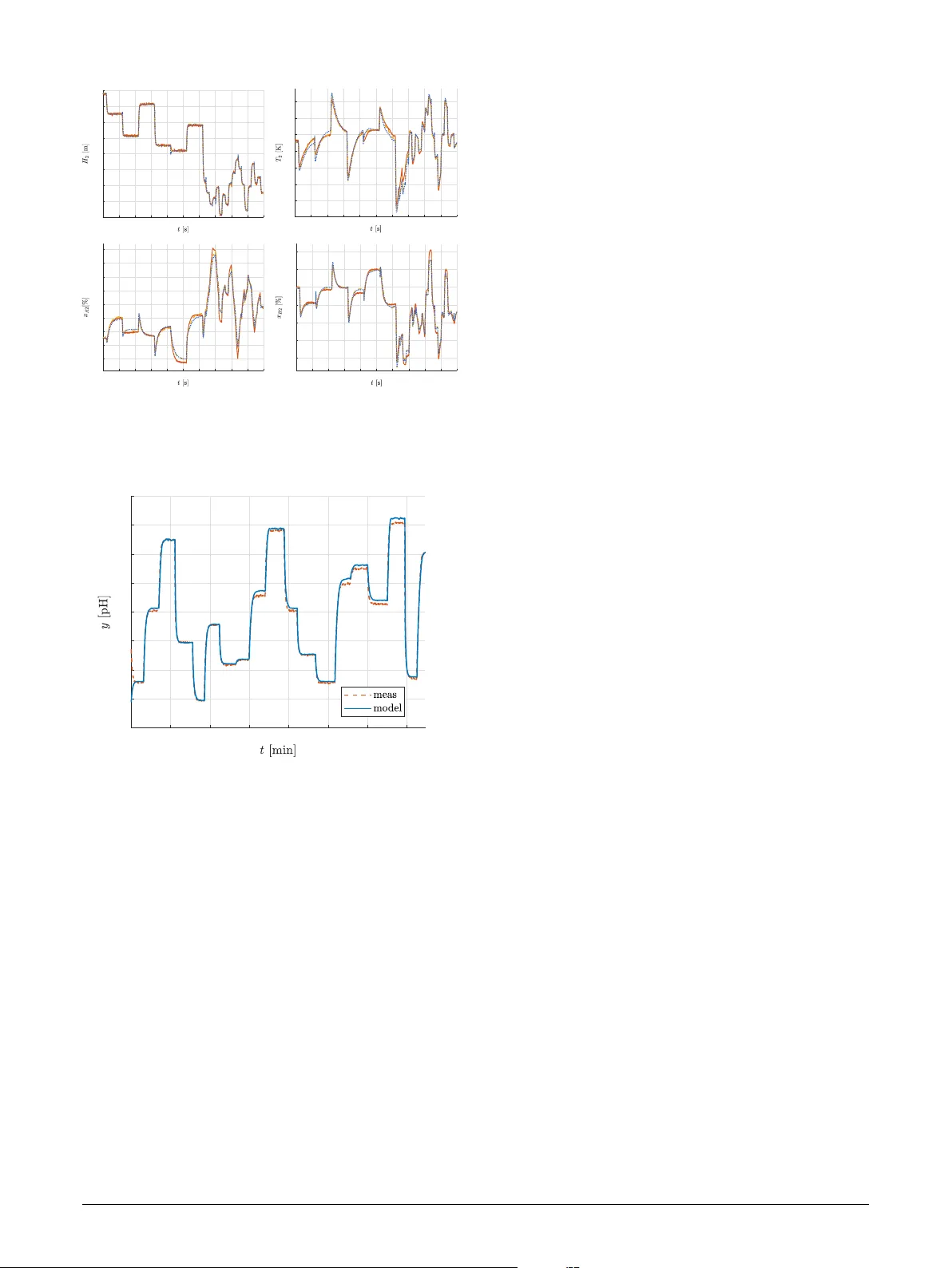
Ph ysics-inf or med str uctured lear ning of a class of recur rent neural netw orks wit h guaranteed properties Daniele Ra v asio a,b , ∗ , Claudia Sbardi a , Marcello Farina a and Andrea Ballarino b a Dipartimento di Elettr onica, Informazione e Bioing egneria (DEIB), P olitecnico di Milano, Via P onzio 34/5, Milan, 20133, Italy b Istituto di Sistemi e T ecnologie Industriali Intelligenti per il Manifatturier o A vanzato (STIIMA) - Consiglio Nazionale delle Ricerche (CNR), Via A . Cor ti 12, Milan, 20133, Italy A R T I C L E I N F O Keyw ords : Large-scale systems phy sics-informed lear ning recurrent neural networks A B S T R A C T This paper proposes a physics-inf ormed lear ning framework for a class of recurrent neural networks tailored to large-scale and networ ked systems. The approach aims to lear n control-oriented models that preserve the str uctural and stability proper ties of the plant. The learning algor ithm is formulated as a conv ex optimisation problem, allowing the inclusion of linear matr ix inequality constraints to enf orce desired system features. Fur thermore, when the plant exhibits structural modular ity , the re- sulting optimisation problem can be parallelised, requiring communication only among neighbour ing subsystems. Simulation results show the effectiveness of the proposed approach. 1. Introduction 1.1. Motivation The modelling and control of large-scale and netw orked systems (LSSs) composed of multiple interacting subsys- tems is a research area t hat has attracted increasing attention, driven b y the need to manage complex, high-dimensional plants [ 17 , 28 ]. Examples include pow er networks, manufac- turing processes, and transpor tation systems. Within this set- ting, centralised control strategies are of ten inadequate due to scalability issues, communication constraints, and pr ivacy concerns. A common approach to address t hese challeng es is to exploit t he str uctural modular ity of t he plant to decompose the ov erall contr ol problem into smaller , w eakl y coupled subproblems, each managed by a local controller , leading to decentralised or distributed control architectures [ 23 ]. How e ver , the design of decentralised or distr ibuted contr ol schemes relies on the av ailability of accurate plant models that exhibit a str ucture consistent with t he intended decom- posed control system architecture [ 28 , 10 ]. The definition of first-pr inciples models f or LSSs of- ten becomes impractical due to their high dimensionality and complexity . In this context, recurrent neural netw orks (RNNs) [ 16 ] ha v e emerged as po werful tools f or modelling complex plants, owing to their ability to capture long-term and nonlinear temporal dependencies directly from data. Ne vertheless, purely black -box models may fail to capture the underl ying comprehensive phy sical/structural properties of t he real system. This lack of physical consistency may result in unreliable or non-interpretable models, which might be inadequate f or control design. This limitation has moti- vated recent research on nov el techniques [ 2 , 11 ] aimed at incorporating prior physical know ledge, such as structural inf ormation, directly into the model training process. ∗ Corresponding author daniele.ravasio@polimi.it (D. Ravasio); claudia.sbardi@mail.polimi.it (C. Sbardi); marcello.farina@polimi.it (M. Far ina); andrea.ballarino@stiima.cnr.it (A. Ballar ino) Besides structural proper ties, when the plant e xhibits properties such as input-to-state stability (ISS, [ 26 ]) or incre- mental ISS ( 𝛿 ISS, [ 1 ]), it is desirable to enf orce t hem to the RNN model. Enforcing stability proper ties at the lear ning stage is relevant from tw o complement ar y perspectiv es [ 2 ]. First, from a physical perspective, it aims to ensure con- sistency with pr ior know ledge of the plant qualitative be- ha viour, thereby improving the reliability and inter pretabil- ity of the obtained model. Second, from a control-oriented perspective, it provides a theoretical tool that can be directly lev erag ed dur ing control design. This idea has been explored in sever al works for the design of control schemes with stability and performance guarantees (see, e.g., [ 3 , 24 ]). The 𝛿 ISS, in par ticular, is a robust stability property t hat guar- antees t he existence of robust positivel y inv ariant sets [ 1 ], which are essential ing redients in the design of robust control algorit hms [ 21 , 20 ]. An impor tant challenge is that standard RNN training techniq ues are generall y centralised and computationally de- manding [ 14 ], which makes them unsuitable for LSSs char - acterised by high dimensionality and, in some cases, lim- ited a vailability of measurements from all subsystems. This limitation ma y stem, f or example, from pr ivacy concer ns or from t he geographical distr ibution of the subsys tems. In addition, str uctural changes in the plant, such as modification of communication constraints, maintenance inter ventions, or component failur es, can require reconfigurability of both t he model and the contr oller [ 17 ]. These issues highlight the need for faster and scalable model learning strategies t hat can operate in a distributed manner at the subsystem lev el. 1.2. Statement of the problem In this wor k we assume t hat the dynamic plant/system  under analy sis is endow ed with manipulable inputs, col- lected in the input vector 𝑢 ∈ ℝ 𝑚 , and measurable outputs, collected in the output vector 𝑦 ∈ ℝ 𝑝 . The aim of this wor k is to develop a framew ork for learning a phy sics- inf ormed recurrent neural netw ork model of the plant  , in which selected phy sical f eatures of t he system are directly Daniele Ravasio et al.: Preprint submitted to Elsevier Page 1 of 16 𝑦 2 𝒫 2 𝑢 2 𝑢 𝑢 1 𝒫 1 𝑦 1 𝑦 𝒫 Figure 1: Mo dula r system structure for a simple case where 𝑛 s = 2 . embedded in the learning process. Concer ning the av ailable data, we make the follo wing assumption. Assumption 1. An informative dataset of input-output data pr eviously collected from the system  is available. The data consists of an applied input sequence  d = { 𝑢 d ( 𝑘 )} 𝑁 d 𝑘 =1 , wher e the scalar 𝑁 d r epr esents the sequence length, and a measur ed output sequence  d = { 𝑦 d ( 𝑘 )} 𝑁 d 𝑘 =1 . The resulting model is intended to provide an accurate representation suitable for control design. The f ocus is on two key aspects: (i) t he construction of a modular model inspired by t he plant str ucture, which can be directly used in the synthesis of a distributed or a decentralised control scheme, and (ii) the incor poration of stability guarantees, so that the resulting model inher its t he stability proper ties of  . 1.2.1. Im posing the modular plant structure Many larg e-scale and complex plants are characterised by a structural modularity which can be un veiled by physi- cal inspection or through data-driven approac hes (see, e.g., [ 18 ]). In particular, we can often define a number 𝑛 s of subplants  𝑖 , where 𝑖 ∈  = {1 , … , 𝑛 s } , each characterised by a local manipulable input vector 𝑢 𝑖 ∈ ℝ 𝑚 𝑖 and a vector 𝑦 𝑖 ∈ ℝ 𝑝 𝑖 of local measurable outputs. In this work w e assume that  𝑛 s 𝑖 =1 𝑚 𝑖 = 𝑚 and  𝑛 s 𝑖 =1 𝑝 𝑖 = 𝑝 , in such a w ay that 𝑢 and 𝑦 are partitioned in a non-ov erlapping fashion, i.e., 𝑢 =  𝑢 ⊤ 1 … 𝑢 ⊤ 𝑛 s  ⊤ 𝑦 =  𝑦 ⊤ 1 … 𝑦 ⊤ 𝑛 s  ⊤ W e assume here that ph ysical interconnections among sub- plants can also be defined, see, e.g., Figure 1 . In general, we sa y t hat t he subplant  𝑗 has a direct influence on (or, in a g raph-theoretical ter minology , is neighbor of) subplant  𝑖 (with 𝑖 ≠ 𝑗 ) if t here e xists an interconnection vector 𝜈  𝑖𝑗 of variables of  𝑗 which is an input f or  𝑖 . V ector 𝜈  𝑖𝑗 ma y include entr ies of 𝑢 𝑗 and of 𝑥 𝑗 , t he latter defining the inter nal state of  𝑗 (some of whose elements may be measurable, i.e., included in 𝑦 𝑗 ). This induces t he definition of t he graph   = {  ,   } , whose edges cor respond to the subplants  𝑖 f or all 𝑖 ∈  , and the pair ( 𝑖, 𝑗 ) is a vertex (i.e., ( 𝑖, 𝑗 ) ∈   ) if and only if 𝜈  𝑖𝑗 ≠ 0 . More specifically , f or all 𝑖 ∈  we can define the f ollo wing neighboring sets:   𝑢,𝑖 ≔ { 𝑗 ∈  ⧵ { 𝑖 } ∶ 𝜈  𝑖𝑗 ≠ 0 includes entries of 𝑢 𝑗 } and   𝑥,𝑖 ≔ { 𝑗 ∈  ⧵ { 𝑖 } ∶ 𝜈  𝑖𝑗 ≠ 0 includes entries of 𝑥 𝑗 } . In Section 4 we propose a methodology to identify 𝑛 s sub- models  𝑖 , with 𝑖 = 1 , … , 𝑛 s , each endow ed with an input/output pair ( 𝑢 𝑖 , 𝑦 𝑖 ) , and interconnected with each other through an interconnection topology induced by the modular system structure defined abov e. Note that, even in model-based contexts, the model decom- position problem is crucial and critical. In fact, as anal- ysed, e.g., in [ 10 ], while over lapping decompositions lead to higher -order submodels  𝑖 with dense (e.g., all-to-all) interconnection structures, non-over lapping decompositions typically lead to submodels  𝑖 with reduced orders and minimal interconnection structures (which may , unless we perform fur ther simplifications, cor respond to the plant real interconnection str uctures). In view of the better scalability of t he latter decomposition, in Section 4 we propose a data- based counter par t of non-ov erlapping decompositions where we lear n submodels, par tially coupled through inputs and/or internal s tates, reflecting t he interconnection graph of the real plant. 1.2.2. Im posing stability guarantees When the plant  enjoy s cer tain stability properties, it is desirable to enforce t he same proper ties on the model. The stability proper ties of  may be deduced from the qualitative beha viour of the plant or inferred numer ically from av ailable input-output data. In this work, in view of the f act that we cast the lear ning problem as a conv e x optimisation one, we can enfor ce the stability proper ties exhibited by the plant through suitable constraints expressed in the form of linear matr ix inequal- ities (LMIs) [ 4 ]. In Section 5 we propose an LMI-based sufficient condition on the weights of the considered model class that guarantees its 𝛿 ISS and exploit this condition to enforce this property , dur ing the learning phase, on the model. Notabl y , when the plant is characterised by a modular structure, the proposed methodology can be lev eraged to impart the 𝛿 ISS proper ty both to t he local submodels  𝑖 , 𝑖 = 1 , … , 𝑛 𝑠 , and to the ov erall structured model resulting from their interconnection. Note that, alt hough in this work we consider t he 𝛿 ISS property , the gener al methodology proposed in Section 5 is not limited to t his setting and can be extended to enforce alternative properties, provided that suitable conditions on the weights of the considered RNN model class can be expressed in ter ms of LMIs. 1.3. State of the art The inclusion of physical know ledge in the definition of learning strategies for RNN models has received consider- able attention in the literature as an attempt to ov ercome the limitations of black -bo x modelling. Along t his line of research, sev eral phy sics-inf ormed approaches ha v e been dev eloped within standard gradient-based training frame- wor ks [ 2 , 11 , 5 ]. One of the most widely adopted approac hes to incor po- rate physical constraints consists in augmenting t he train- ing objective with suit ably designed regular isation ter ms. Daniele Ravasio et al.: Preprint submitted to Elsevier P age 2 of 16 Phy sics-guided loss functions can be designed to enforce phy sical law s such as conservation pr inciples or stability inequalities. With specific reference to stability proper ties, this strategy has been employ ed to enforce ISS and 𝛿 ISS conditions in various RNN architectures [ 2 ]. How e ver , this approach suffers from sev eral limit ations [ 15 ]. First of all, t he conditions to be imposed on the model parameters to impart stability are commonly par ticularly conservative, often compromising the quality of the so- obtained learned models. Also, since t he t hese conditions are not enforced as str ict constraints, there are no guarantees that the resulting model will satisfy the desired physical properties, necessitating a posterior i v erification. Addition- ally , if not designed appropr iately , these regularisation ter ms ma y lead to optimisation issues or to a deg radation of the modelling accuracy . Finally , finding a trade-off between modelling performance and the satisfaction of the physical conditions can be non-trivial and typically in vol v es tr ial- and-er ror tuning. A not able class, essentially different from the ones ad- dressed in the latter works, is represented by the class of recurrent equilibrium netw orks (RENs) introduced in [ 22 ]. These models admit a direct parameter isation that allow s contractivity and robust stability guarantees to be enforced without the need to introduce additional penalty ter ms in the loss function. Ho we ver , t he approach proposed in [ 22 ] may become difficult to apply when one seek s to impose specific structural constraints on t he model matr ices, for instance to reflect the interconnection topology of a larg e-scale plant. An alter native to physics-guided loss functions consists of defining a-pr ior i model classes which embed physical pr ior know ledge. Phy sics-guided architectures can be constr ucted by exploiting the intr insic modular ity of RNNs to enforce consistency wit h phy sical properties such as monotonicity or zero-sum constraints. This approach is particularly relev ant when the data-generating plant exhibits a modular str ucture. In t his case, the underlying structural inf or mation can be reflected in the model by adopting a sparsely connected RNN that is consistent wit h the system topology . This approach has been in ves tigated in [ 29 ] for enf orcing str uctural prop- erties in chemical flow sheet models and in [ 2 ] for lear ning a structured RNN model of a chemical process. How e ver , gradient-based training strategies are gener ally inherently non-conv ex and prone to t he presence of local minima. Moreov er , t hey suffer from significant scalability limitations, as widely adopted methods such as backpr op- ag ation through time typically rely on centralised imple- mentations and are difficult to parallelise [ 16 , 14 ]. This can restrict their applicability to larg e-scale systems, where computational and memory requirements grow rapidly with the system size, potentially resulting in t he so-called curse of dimensionality [ 11 ]. 1.4. Paper objectives and structure Motiv ated by the considerations made in the previous sections, in t his work we propose a novel learning framew ork f or RNNs having the structure of REN models. In par ticular , inspired by the approach proposed in [ 13 ] in t he case of echo state netw orks (ESNs), we adopt a computationally lightweight g radient-free method which relies on a least- squares minimisation problem or , in case of noisy data, on a set-membership approach extending the work proposed in [ 8 ] in several directions. Import antly , in this wor k we apply t his approach to the identification of control-or iented models that preser ve t he structural and stability proper ties of t he plant. The lear ning algor ithm is f ormulated as a con ve x optimisation problem, allowing the inclusion of LMI constraints to enf orce desired sys tem f eatures. Impor t antly , when the plant exhibits structural modular ity , the resulting optimisation problem can be parallelised, requiring commu- nication only among neighbour ing subsystems and resulting scalable and numerically well suited to t ackle large-scale and structured plants. The paper is structured as follo ws. In Section 2 we first define the considered model class, its f eatures, as well as its well-posedness property . Then, in Section 3 we define the main approaches used for well-posed model training; these approaches are exploited in Sections 4 and 5 in case we need to identify models wit h a plant-inspired modular structure and with embedded guaranteed stability proper ties, respectivel y . Simulation tests are reported in Section 6 and conclusions are dra wn in Section 7 . Ev entually , for clar ity of exposition, all proofs are repor ted in the Appendix. 1.5. Notation and preliminaries Given a vector 𝑣 ∈ ℝ 𝑛 , 𝑣 ( 𝑖 ) denotes its 𝑖 -th entr y . Given a matrix 𝑀 ∈ ℝ 𝑛 × 𝑛 , 𝑀 ( 𝑖 ) denotes its 𝑖 -th row , and 𝑀 ⊤ its traspose. Let ℤ + denote the set of positive integers (ex clud- ing zero), 𝕊 𝑛 + the set of real symmetr ic positive definite ma- trices, and 𝔻 𝑛 + the set of real diagonal positive definite matr i- ces. W e denote the sequence ( 𝑢 (0) , … , 𝑢 ( 𝑁 )) by { 𝑢 ( 𝑘 )} 𝑁 𝑘 =0 . The matr ix 𝐼 𝑛 denotes the 𝑛 × 𝑛 identity matr ix. Given 𝑛 matrices 𝑀 1 , … , 𝑀 𝑛 , we denote by diag( 𝑀 1 , … , 𝑀 𝑛 ) the block -diagonal matr ix wit h 𝑀 1 , … , 𝑀 𝑛 on its main diagonal blocks. Given an index set  = {1 , … , 𝑛 } ⊆ ℤ + , its cardinal- ity is denoted by    . Assuming that all matrices 𝑀 𝑖 ha ve t he same number of row s, we define [ 𝑀 𝑖 ] 𝑖 ∈  ≔ [ 𝑀 𝑖 1 … 𝑀 𝑖 𝑛 ] . Consider two index sets  ,  ⊆ {1 , … , 𝑛 } and a matr ix 𝑀 , which is partitioned into 𝑛 × 𝑛 non-ov erlapping blocks 𝑀 𝑖,𝑗 . W e denote this block par tition by 𝑀 = [ 𝑀 𝑖,𝑗 ] 𝑖 ∈  ,𝑗 ∈  . Also, we denote by ( 𝑀 )  ,  the matr ix obt ained by keeping only the ro w-bloc ks of 𝑀 index ed by  and the column- blocks index ed by  . Given a vector 𝑣 partitioned into 𝑚 non-ov erlapping subv ectors 𝑣 𝑖 , 𝑖 = 1 , … , 𝑚 , we denote by ( 𝑣 )  the vector obtained by keeping only the subvectors 𝑣 𝑖 such that 𝑖 ∈  . Giv en a v ector 𝑣 ∈ ℝ 𝑚 and a set   ⊆ ℝ 𝑚 , we define the function dist ( 𝑣,   ) = min  𝑣 ∈    𝑣 −  𝑣  2 A continuous function 𝛼 ∶ ℝ ≥ 0 → ℝ ≥ 0 is a class  -function if 𝛼 ( 𝑠 ) > 0 f or all 𝑠 > 0 , it is str ictly increasing and 𝛼 (0) = 0 . Also, a continuous function 𝛼 ∶ ℝ ≥ 0 → ℝ ≥ 0 is a class  ∞ - function if it is a class  -function and 𝛼 ( 𝑠 ) → ∞ as 𝑠 → ∞ . Finally , a continuous function 𝛽 ∶ ℝ ≥ 0 × ℤ ≥ 0 → ℝ ≥ 0 is a class  -function if 𝛽 ( 𝑠, 𝑘 ) is a class  -function with respect to 𝑠 for all 𝑘 , it is str ictly decreasing in 𝑘 for all 𝑠 > 0 , Daniele Ravasio et al.: Preprint submitted to Elsevier P age 3 of 16 and 𝛽 ( 𝑠, 𝑘 ) → 0 as 𝑘 → ∞ for all 𝑠 > 0 . Consider a general nonlinear discrete-time system descr ibed by , 𝑥 ( 𝑘 + 1) = 𝑓 ( 𝑥 ( 𝑘 ) , 𝑢 ( 𝑘 )) (1) where 𝑘 ∈ ℤ ≥ 0 is the discrete-time index, 𝑥 ∈ ℝ 𝑛 is the state vector , 𝑢 ∈ ℝ 𝑚 is the input vector , and 𝑓 ∶ ℝ 𝑛 × ℝ 𝑚 → ℝ 𝑛 . W e introduce t he follo wing definitions [ 22 , 1 ]. Definition 1. System ( 1 ) is said to be contr acting with r ate 𝛼 ∈ (0 , 1) if, for any two initial conditions 𝑥 𝑎 (0) , 𝑥 𝑏 (0) ∈ ℝ 𝑛 , given the same sequence { 𝑢 ( 𝑘 )} 𝑁 𝑘 =0 , where 𝑁 ∈ ℤ + , the state sequences 𝑥 𝑎 ( 𝑘 ) , 𝑥 𝑏 ( 𝑘 ) satisfy,  𝑥 𝑎 ( 𝑘 ) − 𝑥 𝑏 ( 𝑘 )  ≤ 𝜌𝛼 𝑘  𝑥 𝑎 (0) − 𝑥 𝑏 (0)  , for some 𝜌 ∈ ℝ + . □ Definition 2. System ( 1 ) is said to be 𝛿 ISS with respect to  ⊆ ℝ 𝑛 and  ⊆ ℝ 𝑚 if  is robust positively invariant for ( 1 ) and ther e exist functions 𝛽 ∈  and 𝛾 ∈  ∞ such that for any 𝑘 ∈ ℤ ≥ 0 , any pair of initial states 𝑥 𝑎 (0) , 𝑥 𝑏 (0) ∈  , and any pair of input 𝑢 𝑎 , 𝑢 𝑏 ∈  , it holds that  𝑥 𝑎 ( 𝑘 ) − 𝑥 𝑏 ( 𝑘 )  ≤ 𝛽 (  𝑥 𝑎 (0) − 𝑥 𝑏 (0)  , 𝑘 ) + 𝛾 (max ℎ ≥ 0  𝑢 𝑎 ( ℎ ) − 𝑢 𝑏 ( ℎ )  ) . □ Definition 3. A function 𝑉 ( 𝑥 𝑎 , 𝑥 𝑏 ) is a dissipation-form 𝛿 ISS Lyapunov function for system ( 1 ) if  is robust posi- tivel y inv ariant for ( 1 ) and ther e exist  ∞ -functions 𝛼 1 , 𝛼 2 and 𝛼 3 , and a  -function 𝛼 4 such that, for any pair of states 𝑥 𝑎 ( 𝑘 ) ∈  and 𝑥 𝑏 ( 𝑘 ) ∈  , and any pair of inputs 𝑢 𝑎 ( 𝑘 ) ∈  and 𝑢 𝑏 ( 𝑘 ) ∈  , it holds that 𝛼 1 (  𝑥 𝑎 ( 𝑘 )− 𝑥 𝑏 ( 𝑘 )  ) ≤ 𝑉 ( 𝑥 𝑎 ( 𝑘 ) , 𝑥 𝑏 ( 𝑘 )) ≤ 𝛼 2 (  𝑥 𝑎 ( 𝑘 )− 𝑥 𝑏 ( 𝑘 )  ) , 𝑉 ( 𝑥 𝑎 ( 𝑘 + 1) , 𝑥 𝑏 ( 𝑘 + 1)) − 𝑉 ( 𝑥 𝑎 ( 𝑘 ) , 𝑥 𝑏 ( 𝑘 )) ≤ − 𝛼 3 (  𝑥 𝑎 ( 𝑘 ) − 𝑥 𝑏 ( 𝑘 )  ) + 𝛼 4 (  𝑢 𝑎 ( 𝑘 ) − 𝑢 𝑏 ( 𝑘 )  ) . □ A sufficient condition such t hat system ( 1 ) is 𝛿 ISS is stated in the follo wing theorem [ 1 ]. Theorem 1. If syst em ( 1 ) admits a dissipation-form 𝛿 ISS Lyapuno v function ov er the sets  and  , then it is 𝛿 ISS with respect to such sets, in the sense of Definition 2 . □ 2. The selected recurr ent neural netw or k class 2.1. The recurrent neural networ k model The RNN considered in this paper is a deep (i.e., multi- la yer) architecture comprising 𝑛 neurons in the reservoir , whose states are collected in the vector 𝑥 ∈ ℝ 𝑛 . The RNN takes an input 𝑢 ∈ ℝ 𝑚 and produces an output 𝑦 ∈ ℝ 𝑝 . In order to simplify the lear ning process, we adopt a training approach inspired by the ESN training algorit hm proposed in [ 13 ]. Accordingl y , the RNN model is descr ibed as 𝑥 ( 𝑘 + 1) = 𝐴 𝑥 𝑥 ( 𝑘 ) + 𝐵 𝑢 𝑢 ( 𝑘 ) + 𝐵 o 𝑠 𝑠 ( 𝑘 ) + 𝐵 𝑦 𝑦 ( 𝑘 ) (2a) 𝑠 ( 𝑘 ) = 𝜎 (  𝐴 𝑥 𝑥 ( 𝑘 ) +  𝐵 𝑢 𝑢 ( 𝑘 ) +  𝐵 o 𝑠 𝑠 ( 𝑘 ) +  𝐵 𝑦 𝑦 ( 𝑘 )) (2b) 𝑦 ( 𝑘 ) = 𝐶 𝑥 ( 𝑘 ) + 𝐷 𝑢 ( 𝑘 ) + 𝐷 𝑠 𝑠 ( 𝑘 ) (2c) Matrices 𝐴 𝑥 ∈ ℝ 𝑛 × 𝑛 , 𝐵 𝑢 ∈ ℝ 𝑛 × 𝑚 , 𝐵 o 𝑠 ∈ ℝ 𝑛 × 𝜈 , 𝐵 𝑦 ∈ ℝ 𝑛 × 𝑝 ,  𝐴 𝑥 ∈ ℝ 𝜈 × 𝑛 ,  𝐵 𝑢 ∈ ℝ 𝜈 × 𝑚 ,  𝐵 o 𝑠 ∈ ℝ 𝜈 × 𝜈 , and  𝐵 𝑦 ∈ ℝ 𝜈 × 𝑝 are treated as hyper parameters, which are selected bef ore training. On the other hand, matr ices 𝐶 ∈ ℝ 𝑛 × 𝑝 , 𝐷 ∈ ℝ 𝑝 × 𝑚 , and 𝐷 𝑠 ∈ ℝ 𝑝 × 𝜈 are free trainable parameters. Moreov er , 𝜎 ( ⋅ ) ∶ ℝ 𝜈 → ℝ 𝜈 is a decentralised vector of sigmoidal activation functions applied element-wise, i.e., 𝜎 ( 𝑣 ) =  𝜎 (1) ( 𝑣 (1) ) … 𝜎 ( 𝜈 ) ( 𝑣 ( 𝜈 ) )  ⊤ , where 𝜎 ( 𝑖 ) ( ⋅ ) , f or 𝑖 = 1 , … , 𝜈 , are h yper parameters that must be selected so as to fulfil the follo wing assumption. Assumption 2. Each component 𝜎 ( 𝑖 ) ∶ ℝ → ℝ , 𝑖 = 1 , … , 𝜈 , is a sigmoid function, i.e., a bounded, twice con- tinuously differentiable function with positive first derivative at eac h point and one and only one inflection point in 𝜎 ( 𝑖 ) (0) = 0 . Also, 𝜎 ( 𝑖 ) ( ⋅ ) is Lipschitz continuous with unitar y Lipschitz constant and suc h that 𝜎 ( 𝑖 ) (0) , 𝜕 𝜎 ( 𝑖 ) ( 𝑣 ( 𝑖 ) ) 𝜕 𝑣 ( 𝑖 )    𝑣 ( 𝑖 ) =0 = 1 and 𝜎 ( 𝑖 ) ( 𝑣 ( 𝑖 ) ) ∈ [−1 , 1] , ∀ 𝑣 ( 𝑖 ) ∈ ℝ . 2.2. Hyperparameters definition Similarl y to the ESN training algor ithm [ 13 ], the hyper - parameters 𝑛 (i.e., the RNN order), 𝜈 (i.e., the number of entries of 𝑠 ), 𝜎 ( 𝑖 ) (the nonlinear ity type), for 𝑖 = 1 , … , 𝜈 , and the matr ices in ( 2a )-( 2b ) are user-generated before training. In par ticular, matr ices ( 𝐵 𝑢 , 𝐵 𝑜 𝑠 , 𝐵 𝑦 ,  𝐵 𝑢 ,  𝐵 𝑦 ) can take random values. On the other hand, matr ices ( 𝐴 𝑥 ,  𝐴 𝑥 ,  𝐵 o 𝑠 ) must be defined according to t he follo wing proposition [ 22 ]. Proposition 1. Under Assumption 2 , if there exist  𝛼 ∈ (0 , 1) and matrices 𝑃 o ∈ 𝕊 𝑛 + and Λ o ∈ 𝔻 𝜈 + , such that   𝛼 2 𝑃 o −  𝐴 ⊤ 𝑥 Λ o −Λ o  𝐴 𝑥 2Λ o − Λ o  𝐵 o 𝑠 −  𝐵 o ⊤ 𝑠 Λ o  −  𝐴 ⊤ 𝑥 𝐵 o 𝑠 ⊤  𝑃 o  𝐴 𝑥 𝐵 o 𝑠  ≻ 0 , (3) then, model ( 2 ) is well-posed and contr acting with r ate 𝛼 <  𝛼 . □ Note that, b y appl ying t he Schur complement to ( 3 ) and by substituting 𝑍 𝑥 = 𝑃 o 𝐴 𝑥 ,  𝑍 𝑥 = Λ o  𝐴 𝑥 , and  𝑍 𝑠 = Λ o  𝐵 o 𝑠 , condition ( 3 ) is equivalent to      𝛼 2 𝑃 o −  𝑍 ⊤ 𝑥 𝑍 ⊤ 𝑥 −  𝑍 𝑥 2Λ o −  𝑍 𝑠 −  𝑍 ⊤ 𝑠 𝐵 o 𝑠 ⊤ 𝑃 o 𝑍 𝑥 𝑃 o 𝐵 o 𝑠 𝑃 o     ≻ 0 , (4) Theref ore, contractivity and well-posedness of the untrained model ( 2 ) can be guaranteed by solving the LMI ( 4 ) with decision variables 𝑃 o ∈ 𝕊 𝑛 + , Λ o ∈ 𝔻 𝜈 + , 𝑍 𝑥 ∈ ℝ 𝑛 × 𝑛 ,  𝑍 𝑥 ∈ ℝ 𝜈 × 𝑛 , and  𝑍 𝑠 ∈ ℝ 𝜈 × 𝜈 , and then setting 𝐴 𝑥 = 𝑃 −1 o 𝑍 𝑥 , Daniele Ravasio et al.: Preprint submitted to Elsevier P age 4 of 16  𝐴 𝑥 = Λ −1 o  𝑍 𝑥 , and  𝐵 o 𝑠 = Λ −1 o  𝑍 𝑠 . Note that t he contractivity property plays the same role as the echo state proper ty in [ 13 ]. In par ticular, this property is impor tant dur ing training, as it guarantees that the state trajectories of ( 2 ) asymptoticall y depend only on the dr iving input signals ( 𝑢, 𝑦 ) , while the effect of the initial conditions vanishes asymptoticall y o ver time. Thanks to t his prop- erty , we can le verag e the linear-in-the-parameters str ucture of ( 2c ) with respect to t he free parameters to formulate the learning problem as a con ve x optimisation problem. A general drawbac k of the proposed approach is that fixing the matr ices in ( 2a )-( 2b ) a pr iori reduces t he number of free parameters, which may lead to low er performance compared with conv entional g radient-based training methods. Note, how e ver , that this limit ation can be mitigated by resor ting to methods f or informed hyper parameter selection, along the lines of [ 25 ]. 2.3. The trained model In this wor k, model ( 2 ) is ref er red to as the untrained model. After the training of t he free parameters 𝐶 , 𝐷 , and 𝐷 𝑠 (see Section 3 for details), one can use the output relation ( 2c ) into ( 2a )-( 2b ) and define 𝐴 = 𝐴 𝑥 + 𝐵 𝑦 𝐶 , 𝐵 = 𝐵 𝑢 + 𝐵 𝑦 𝐷 , 𝐵 𝑠 = 𝐵 o 𝑠 + 𝐵 𝑦 𝐷 𝑠 ,  𝐴 =  𝐴 𝑥 +  𝐵 𝑦 𝐶 ,  𝐵 =  𝐵 𝑢 +  𝐵 𝑦 𝐷 , and  𝐵 𝑠 =  𝐵 o 𝑠 +  𝐵 𝑦 𝐷 𝑠 . In t his wa y , we can rewrite ( 2 ) as 𝑥 ( 𝑘 + 1) = 𝐴𝑥 ( 𝑘 ) + 𝐵 𝑢 ( 𝑘 ) + 𝐵 𝑠 𝑠 ( 𝑘 ) (5a) 𝑠 ( 𝑘 ) = 𝜎 (  𝐴𝑥 ( 𝑘 ) +  𝐵 𝑢 ( 𝑘 ) +  𝐵 𝑠 𝑠 ( 𝑘 )) (5b) 𝑦 ( 𝑘 ) = 𝐶 𝑥 ( 𝑘 ) + 𝐷 𝑢 ( 𝑘 ) + 𝐷 𝑠 𝑠 ( 𝑘 ) (5c) Note that, when  𝐵 𝑠 has a lower tr iangular str ucture, the components of 𝑠 ( 𝑘 ) can be computed explicitl y , row by row , from ( 5b ). Theref ore, model ( 5 ) is w ell-posed by constr uc- tion, i.e., equation ( 5b ) admits a unique solution 𝑠 ( 𝑘 ) for any given pair ( 𝑥 ( 𝑘 ) , 𝑢 ( 𝑘 )) . In t he general case in which  𝐵 𝑠 is full, as discussed in [ 22 , 19 ], a sufficient condition for model ( 5 ) to be also well-posed is the existence of a matr ix Λ ∈ 𝔻 𝜈 + such that 2Λ − Λ  𝐵 𝑠 −  𝐵 𝑠 Λ ⊤ ≻ 0 . (6) Notabl y , ( 6 ) will be imposed, through the inclusion of suit- able matr ix inequalities, in the training procedure. 3. Learning unstructured models As discussed, the approach proposed in this section is inspired by the one proposed in [ 13 ] f or ESNs. In par tic- ular, consider ing model ( 2 ), t he hyperparameters are pre- viously defined and only matrices 𝐶 , 𝐷 , and 𝐷 𝑠 are free training parameters. For notational reasons, we define 𝜃 =  𝐶 𝐷 𝐷 𝑠  ∈ ℝ 𝑝 × 𝑟 . The advantage of this approach is that of reducing the train- ing problem to a conv ex and comput ationally lightweight one, which can be optimally solved using standard conv e x optimisation techniq ues. In this section we present two al- ternative procedures for training unstr uctured models. First, the algor ithm described in Section 3.1 is based on the f ormulation of the lear ning problem as a least-squares minimisation. Howe v er , in real-w orld applications, the out- put data are of ten subject to uncer tainty , which can affect the accuracy of the estimated parameters. Specifically , when noise is present, t he least-squares approach may no longer pro vide cor rect and consistent estimates due to the possi- ble cor relation of the noise in t he output equation. As a result, the least-squares estimator 𝜃 LS can become biased, potentiall y deg rading the resulting model per f ormance. For this reason, inspired by [ 8 , 25 ], in Section 3.2 we provide an alter native approach based on set-membership which, among other t hings, does not need any assumption on t he noise probability distribution. 3.1. Least-squar es learning procedur e The identification of 𝜃 can be performed according to Algorit hm 1 . Note t hat the procedure descr ibed in Algorit hm 1 does not Algorithm 1 Least-squares learning 1: Simulate ( 2a )–( 2b ) from a random initial condition 𝑥 (0) , using the dataset input sequence  d and output sequence  d . This yields the trajectories { 𝑥 d ( 𝑘 )} 𝑁 d 𝑘 =1 and { 𝑠 d ( 𝑘 )} 𝑁 d 𝑘 =1 , which repre- sent t he evolution of t he variables 𝑥 ( 𝑘 ) and 𝑠 ( 𝑘 ) , respectivel y . 2: Define Φ ≔     𝑥 d ( 𝜏 w + 1) ⊤ 𝑢 d ( 𝜏 w + 1) ⊤ 𝑠 d ( 𝜏 w + 1) ⊤ ⋮ ⋮ ⋮ 𝑥 d ( 𝑁 d ) ⊤ 𝑢 d ( 𝑁 d ) ⊤ 𝑠 d ( 𝑁 d ) ⊤     , 𝑌 d ≔     𝑦 d ( 𝜏 w + 1) ⊤ ⋮ 𝑦 d ( 𝑁 d ) ⊤     , where the washout period 𝜏 w ∈ ℤ + is an additional hyper pa- rameter introduced to accommodate the initial model transient due to the random initialisation. 3: Compute the solution 𝜃 ⋆ to t he least-squares problem 𝜃 ⋆ = ar g min 𝜃 𝐽 ( 𝜃 ) , 𝐽 ( 𝜃 ) = 1 𝑁 d − 𝜏 w   𝑌 d − Φ 𝜃 ⊤   2 . (7) guarantee, in general, the well-posedness of the model ( 5 ). In pr inciple, this proper ty could be enforced by minimising 𝐽 ( 𝜃 ) while, at the same time, imposing the well-posedness condition ( 6 ). Howe v er, this results in a bilinear optimisation problem, which can be computationally intensive and prone to numer ical issues. T o obtain a tractable formulation of this problem, w e intro- duce the follo wing proposition. Proposition 2. The optimisation problem min 𝑠 ∈ ℝ + ,𝐻 ∈ ℝ 𝑝 × 𝑟 𝑠, subject to:  𝑠 𝐻 − ( 𝑄 −1 d Φ ⊤ 𝑌 d ) ⊤  𝑄 𝐻 ⊤ −  𝑄𝑄 −1 d Φ ⊤ 𝑌 d  𝑄  ⪰ 0 (8a) Daniele Ravasio et al.: Preprint submitted to Elsevier P age 5 of 16 wher e 𝑄 d = Φ ⊤ Φ and 𝜃 ⋆ = 𝐻  𝑄 −1 , is equivalent to ( 7 ) , if, for any 𝛾 ∈ ℝ + ,  𝑄 = 𝛾 𝑄 d . (9) Mor eov er , define matr ices 𝐻 e ∈ ℝ 𝑝 × 𝑛 + 𝑚 and 𝐻 𝑠 ∈ ℝ 𝑝 × 𝜈 such that 𝐻 =  𝐻 e , 𝐻 𝑠  . If ther e exist matrices  𝑄 e ∈ 𝕊 𝑛 + 𝑚 + and 𝑄 𝑠 ∈ 𝔻 𝜈 + such that  𝑄 = diag(  𝑄 e , 𝑄 𝑠 ) , and the condition 2 𝑄 𝑠 −  𝐵 o 𝑠 𝑄 𝑠 −  𝐵 𝑦 𝐻 𝑠 − 𝑄 𝑠  𝐵 o ⊤ 𝑠 − 𝐻 ⊤ 𝑠  𝐵 ⊤ 𝑦 ≻ 0 , (10) holds, then model ( 5 ) is well-posed. □ The proof of Proposition 2 is provided in the Appendix. This result allow s us to formulate the learning problem of well- posed models as an LMI one. Howe v er , note that the equality condition ( 9 ) is optimal f or training, but it cannot be verified in general, par ticularl y under condition ( 10 ). Inspired by [ 7 ], we relax ( 9 ) by consider ing  𝑄 e and 𝑄 𝑠 as optimisation variables and replacing ( 9 ) with the follo wing inequalities  𝑄 − 1 𝑁 d − 𝜏 w 𝑄 d + 𝜆𝐼 𝑟 ⪰ 0 −  𝑄 + 1 𝑁 d − 𝜏 w 𝑄 d + 𝜆𝐼 𝑟 ⪰ 0 (11) where 𝜆 ∈ ℝ + is a furt her optimisation variable to be minimised. Based on t hese considerations, we can now replace Step 3 of Algorit hm 1 with Algor ithm 2 . Specifically , we compute 𝜃 ⋆ as 𝜃 ⋆ = W ellP osed_LS ( 𝑌 d , Φ , 𝑟, 𝜈 , 𝑝, 𝐵 o 𝑠 , 𝜏 w , 𝛽 ) , where 𝛽 ∈ ℝ + is a design parameter . Algorithm 2 W ellP osed_LS Req uire: 𝑌 d , Φ , 𝑟 , 𝜈 , 𝑝 , 𝐵 o 𝑠 , 𝜏 w , 𝛽 Ensure: 𝜃 ⋆ 1: Solve min 𝑠,𝜆 ∈ ℝ + ,  𝑄 e ∈ 𝕊 𝑟 − 𝜈 + , 𝑄 𝑠 ∈ 𝔻 𝜈 + , 𝐻 e ∈ ℝ 𝑝 ×( 𝑟 − 𝜈 ) , 𝐻 𝑠 ∈ ℝ 𝑝 × 𝜈 𝑠 + 𝛽 𝜆 subject to: ( 8a ) , ( 10 ) , ( 11 ) . (12) 2: Set 𝜃 ⋆ = 𝐻  𝑄 −1 , where 𝐻 = [ 𝐻 e , 𝐻 𝑠 ] and  𝑄 = diag(  𝑄 e , 𝑄 𝑠 ) . 3.2. The set membership approac h The algor ithm proposed in this section addresses the case in which biased and inaccurate parameter estimation may result when measurements are affected by additive bounded noise, i.e. 𝑦 d ( 𝑘 ) = 𝑦 ( 𝑘 ) + 𝜂 ( 𝑘 ) . (13) where 𝜂 ( 𝑘 ) verifies t he follo wing. Assumption 3. The noise satisfies  𝜂 ( 𝑘 )  ≤  𝜂 for all 𝑘 ∈ ℤ + , where  𝜂 ∈ ℝ 𝑝 + is known. The main idea behind t his approach, previousl y explored in [ 8 , 25 ] is to str ucture the training into two steps. First we compute the set, ref er red to as the f easible parameter set (FPS), of all model parameterisations consistent with t he a vailable dat a. Then we e xtract from this set the parameter value that satisfies the desired proper ties and achiev es t he best performance on a validation dat aset according to a chosen suitability index. Note also t hat, since our goal is to lear n control-or iented models, the resulting model uncer tainty bound provides valuable information that can be employ ed within robust control schemes, along t he lines of [ 8 ], to account for possi- ble model uncer tainty . In this case we assume also t hat a validation dataset is a vailable, which satisfies the follo wing. Assumption 4. A validation dataset independent from the one used for training is available. This dataset consists of an input sequence  v = { 𝑢 v ( 𝑘 )} 𝑁 v 𝑘 =1 and a measured output sequence  v = { 𝑦 v ( 𝑘 )} 𝑁 v 𝑘 =1 . 3.2.1. Definition of the FPS T o define the FPS, we introduce t he vectors 𝜙 d ( 𝑘 ) ≔ [ 𝑥 d ( 𝑘 ) ⊤ , 𝑢 d ( 𝑘 ) ⊤ , 𝑠 d ( 𝑘 )] ⊤ and 𝜙 ( 𝑘 ) ≔ [ 𝑥 ( 𝑘 ) ⊤ , 𝑢 ( 𝑘 ) ⊤ , 𝑠 ( 𝑘 ) ⊤ ] ⊤ , where 𝑥 d ( 𝑘 ) and 𝑠 d ( 𝑘 ) (respectiv ely , 𝑥 ( 𝑘 ) and 𝑠 ( 𝑘 ) ) are obtained by simulating model ( 2 ) wit h the dat aset sequences (  d ,  d ) (respectively , the ideal sequences { 𝑢 ( 𝑘 ) , 𝑦 ( 𝑘 )} 𝑁 d 𝑘 =0 ). Since 𝑢 ( 𝑘 ) = 𝑢 d ( 𝑘 ) for all 𝑘 , ( 13 ) can be rewritten as 𝑦 ( 𝑖 ) d ( 𝑘 ) = 𝜃 ( 𝑖 ) 𝜙 d ( 𝑘 ) + 𝜖 𝑖 ( 𝑘 ) + 𝜂 ( 𝑖 ) ( 𝑘 ) , f or all 𝑖 = 1 , … , 𝑝 , where 𝜖 𝑖 ( 𝑘 ) = − 𝜃 ( 𝑖 ) 𝑤 d ( 𝑘 ) accounts f or the effect of the measurement noise on t he state predictions, and 𝑤 d ( 𝑘 ) = 𝜙 d ( 𝑘 ) − 𝜙 ( 𝑘 ) =     𝑥 d ( 𝑘 ) − 𝑥 ( 𝑘 ) 0 𝑠 d ( 𝑘 ) − 𝑠 ( 𝑘 )     ∈ ℝ 𝑟 . The follo wing proposition can be pro ved. Proposition 3. Under Assumptions 2 and 3 , if the RNN ( 2 ) satisfies condition ( 3 ) , then: (i) model ( 2 ) is 𝛿 ISS; (ii) ther e exis t functions 𝛽 ∈  and 𝛾 ∈  ∞ such that for any 𝑘 ∈ ℤ + , it holds that  𝑥 d ( 𝑘 )− 𝑥 ( 𝑘 )  ≤  𝑤 𝑥 ( 𝑘 ) ≔ 𝛽 (  𝑥 d (0)− 𝑥 (0)  , 𝑘 )+ 𝛾 (  𝜂 ); (iii) for any 𝑘 ∈ ℤ + , ther e exist Σ( 𝑘 ) ∈ 𝔻 𝜈 + wher e Σ( 𝑘 ) ⪯ 𝐼 𝜈 suc h that  𝑠 d ( 𝑘 ) − 𝑠 ( 𝑘 )  ≤  𝑤 𝑠 ( 𝑘 ) , where  𝑤 𝑠 ( 𝑘 ) ≔  ( 𝐼 𝜈 − Σ( 𝑘 )  𝐵 o 𝑠 ) −1 Σ( 𝑘 )  𝐴 𝑥   𝑤 𝑥 ( 𝑘 ) +  ( 𝐼 𝜈 − Σ( 𝑘 )  𝐵 o 𝑠 ) −1 Σ( 𝑘 )  𝐵 𝑦   𝜂 . Daniele Ravasio et al.: Preprint submitted to Elsevier P age 6 of 16 The proof of Proposition 3 has been postponed to the ap- pendix for clar ity reasons. In the light of it, if the model hyperparameters are chosen as descr ibed in Section 2.2 , t hen  𝜖 𝑖 ( 𝑘 )  ≤  𝜖 𝑖 ≔  𝐶 ( 𝑖 )   𝑤 𝑥 ( 𝑘 ) +  𝐷 ( 𝑖 ) 𝑠   𝑤 𝑠 ( 𝑘 ) f or all 𝑘 ∈ ℤ + and for all 𝑖 = 1 , … , 𝑝 . Exploiting the boundedness of 𝜖 𝑖 , the FPS Θ can be defined f ollowing the procedure outlined in Algorit hm 3 [ 8 ]. The parameter 𝛼 𝑖 in ( 14 ) accounts for t he uncer tainty arising Algorithm 3 FPS_computation Req uire: { 𝑦 d ( 𝑘 )} 𝑁 d 𝑘 = 𝜏 w +1 , { 𝜙 d ( 𝑘 )} 𝑁 d 𝑘 = 𝜏 w +1 , 𝑟 , 𝑝 , 𝜏 w ,  𝜂 Ensure: Θ 1: for 𝑖 = 1 , … , 𝑝 do 2: Solv e the optimisation problem 𝜆 𝑖 = min 𝜆 ∈ ℝ ≥ 0 , 𝐾 ∈ ℝ 𝑟 𝜆 subject to    𝑦 ( 𝑖 ) d ( 𝑘 ) − 𝐾 ⊤ 𝜙 d ( 𝑘 )    ≤ 𝜆 +  𝜂 ( 𝑖 ) , ∀ 𝑘 ∈ { 𝜏 w + 1 , … , 𝑁 d } . 3: Compute   𝜖 𝑖 = 𝛼 𝑖 𝜆 𝑖 , 𝛼 𝑖 > 1 . (14) 4: end for 5: Constr uct the FPS Θ = Θ 1 ( 𝛼 1 ) × ⋯ × Θ 𝑝 ( 𝛼 𝑝 ) , where, for all 𝑘 = 𝜏 w + 1 , … , 𝑁 d , Θ 𝑖 ( 𝛼 𝑖 ) =  𝜃 ( 𝑖 ) ∈ ℝ 1× 𝑟 ∶    𝑦 ( 𝑖 ) d ( 𝑘 ) − 𝜃 ( 𝑖 ) 𝜙 d ( 𝑘 )    ≤   𝜖 𝑖 +  𝜂 ( 𝑖 )  . from the finite number of measurements in the dataset, and satisfies 𝛼 𝑖 → 1 + as 𝑁 d increases. A practical w ay to define 𝛼 𝑖 is to set t his parameter , for all 𝑖 = 1 , … , 𝑝 , at t he minimum value such t hat the least square model parametrisation 𝜃 LS , lies within Θ . In par ticular, we set, f or all 𝑖 = 1 , … , 𝑝 [ 25 ], 𝛼 𝑖 = max 𝑘 ∈{ 𝜏 w +1 , … ,𝑁 d }  𝑦 ( 𝑖 ) ( 𝑘 ) − 𝜃 ( 𝑖 ) LS 𝜙 d ( 𝑘 )  −  𝜂 ( 𝑖 ) 𝜆 𝑖 . (15) If, howe v er, ( 15 ) yields an FPS such t hat 𝜃 LS ∉ Θ , this outcome indicates a possibly incorrect choice of the model class, and t he procedure should therefore be repeated with different hyperparameters. 3.2.2. Scenar io sampling of the FPS No w t hat the FPS is defined, w e need to deter mine the optimal model parameter isation 𝜃 ⋆ ∈ Θ that achie ves t he highest per f ormance on t he validation dataset. How e ver , since exploring all possible values 𝜃 ∈ Θ ma y be computationally intract able, we restrict the analysis to 𝑁 s scenarios 𝜃 [ 𝑡 ] , for 𝑡 = 1 , … , 𝑁 s , drawn from Θ . For each scenar io, model ( 5 ) is simulated using the validation dataset input sequence  v , resulting in the output simulated trajectory { 𝑦 [ 𝑡 ] ( 𝑘 )} 𝑁 v 𝑘 =1 . To assess the model per f ormance of each scenar io, follo wing the approach in [ 8 ], we compute t he minimum distance of t he simulated output of scenar io 𝑡 from the noisy output data tube   ( 𝑘 ) as 𝑑 [ 𝑡 ] ≔ min 𝑘 = 𝜏 w +1 , … ,𝑁 v dist ( 𝑦 [ 𝑡 ] ( 𝑘 ) ,   ( 𝑘 )) , (16) where   ( 𝑘 ) ≔ {  𝑦 ( 𝑘 ) ∈ ℝ 𝑝 ∶   𝑦 ( 𝑖 ) ( 𝑘 )− 𝑦 ( 𝑖 ) v ( 𝑘 )  ≤  𝜂 ( 𝑖 ) , ∀ 𝑖 = 1 , … , 𝑝 } . The optimal parameter value 𝜃 ⋆ is t hen selected as the one associated wit h the minimum distance 𝑑 ⋆ ≔ min 𝑡 =1 , … ,𝑁 s 𝑑 [ 𝑡 ] . The follo wing result provides a cr iterion for selecting t he number of scenarios 𝑁 s [ 8 ]. Proposition 4. Let 𝜃 [ 𝑁 s +1] ∈ Θ be a random matr ix with pr obability distribution ℙ 𝜃 [ 𝑁 s +1] ov er Θ . Also, let 𝜖 ∈ (0 , 1) and 𝛽 ∈ (0 , 1) be two user -defined constants. F or all 𝑁 s ≥ 1 such that 𝑁 s ≥ log 1− 𝜖 ( 𝛽 ) , then with probability 1 − 𝛽 it holds that ℙ { 𝜃 [ 𝑁 s +1] ∈ Θ ∶ 𝑑 [ 𝑁 s +1] < 𝑑 ⋆ } ≤ 𝜖 . How e ver , t his approach does not generally ensure that the model extracted from the FPS satisfies the well-posedness condition ( 6 ). Given 𝜃 [ 𝑡 ] ∈ Θ , t he closest f easible parameter  𝜃 [ 𝑡 ] satisfying ( 6 ) can be computed by solving the LMI problem min { 𝑐 𝑖 ∈ ℝ + } 𝑝 𝑖 =1 ,  𝑄 e ∈ 𝕊 𝑟 − 𝜈 + , 𝑄 𝑠 ∈ 𝔻 𝜈 + , 𝐻 e ∈ ℝ 𝑝 ×( 𝑟 − 𝜈 ) , 𝐻 𝑠 ∈ ℝ 𝑝 × 𝜈 𝑝  𝑖 =1 𝑐 𝑖 (17a) subject to:  𝑐 𝑖 𝜃 [ 𝑡 ] ( 𝑖 )  𝑄 − 𝐻 ( 𝑖 ) ( 𝜃 [ 𝑡 ] ( 𝑖 )  𝑄 − 𝐻 ( 𝑖 ) ) ⊤  𝑄  ⪰ 0 , ∀ 𝑖 = 1 , … , 𝑝 (17b) LMI ( 10 ) and setting  𝜃 [ 𝑡 ] = 𝐻  𝑄 −1 , where 𝐻 = [ 𝐻 e , 𝐻 𝑠 ] and  𝑄 = diag(  𝑄 e , 𝑄 𝑠 ) . Note t hat minimising 𝑐 𝑖 under constraint ( 17b ) is equivalent to minimising the weighted nor m  𝜃 [ 𝑡 ] ( 𝑖 ) −  𝜃 [ 𝑡 ] ( 𝑖 )   𝑄 . The overall set membership lear ning procedure is summarised in Algor ithm 4 . 4. Learning structured models In this section we address the design of a ph ysics- inf ormed procedure to der iv e a modular plant model, where the modular ity is inspired by that of the plant  . In par- ticular, we discuss how to identify a number 𝑛 s of sub- models  𝑖 , each cor responding with a subplant  𝑖 , with 𝑖 = 1 , … , 𝑛 s , each having as local input and output the pair ( 𝑢 𝑖 , 𝑦 𝑖 ) and where interconnections wit h t he other submodels occur t hrough suit able interconnection variables 𝜈  𝑖𝑗 , for 𝑗 ≠ 𝑖 . T o this regard, the main modelling choice lies in t he twof old selection of (i) the model interconnection netw ork, and (ii) the coupling variables. Regar ding (i), we need to define which submodels hav e a direct influence on  𝑖 f or all 𝑖 ∈  , i.e., t he values of 𝑗 ≠ 𝑖 such that 𝜈  𝑖𝑗 ≠ 0 . At the same time, problem (ii) requires to define how 𝜈  𝑖𝑗 , when not identically equal to zero, is composed. For mally speaking, the scope is to define, for all Daniele Ravasio et al.: Preprint submitted to Elsevier P age 7 of 16 Algorithm 4 Set membership lear ning 1: Simulate ( 2a )–( 2b ) from a random initial condition 𝑥 (0) , using the dataset input sequence  d and output sequence  d . This yields t he trajectories { 𝑥 d ( 𝑘 )} 𝑁 d 𝑘 =1 and { 𝑠 d ( 𝑘 )} 𝑁 d 𝑘 =1 . 2: Compute the FPS Θ = FPS_computation ({ 𝑦 d ( 𝑘 )} 𝑁 d 𝑘 = 𝜏 w +1 , { 𝜙 d ( 𝑘 )} 𝑁 d 𝑘 = 𝜏 w +1 , 𝑟, 𝑝, 𝜏 w ,  𝜂 ) . 3: for all 𝑡 = 1 , … , 𝑁 s do 4: Extract a parameter sample 𝜃 [ 𝑡 ] ensuring that the model is well-posed 𝜃 [ 𝑡 ] = W ellPosed_scenario_sampling (Θ , 𝑡, 𝜈 , 𝑝,  𝐵 o 𝑠 ) 5: if  𝜃 [ 𝑡 ] ∉ Θ then 6: Set 𝑑 [ 𝑡 ] = 𝑀 , where 𝑀 is a larg e positive scalar. 7: else 8: Simulate model ( 5 ) using the dataset input sequence  v , resulting in the output trajector y { 𝑦 [ 𝑡 ] ( 𝑘 )} 𝑁 d 𝑘 =1 . 9: Compute 𝑑 [ 𝑡 ] according to ( 16 ). 10: end if 11: end for 12: Select 𝜃 ⋆ = 𝜃 [ 𝑡 ⋆ ] , where 𝑡 ⋆ ≔ ar g min 𝑡 ∈{1 , … ,𝑁 s } 𝑑 [ 𝑡 ] . Algorithm 5 W ellP osed_scenario_sampling Req uire: Θ , 𝑟 , 𝜈 , 𝑝 ,  𝐵 o 𝑠 Ensure:  𝜃 s 1: Randomly extract 𝜃 s from (Θ , ℙ 𝜃 s ) . 2: Solve ( 17 ). 3: Set  𝜃 s = 𝐻  𝑄 −1 , where 𝐻 = [ 𝐻 e , 𝐻 𝑠 ] and  𝑄 = diag(  𝑄 e , 𝑄 𝑠 ) . 𝑖 ∈  , t he neighbor ing sets:   𝑢,𝑖 ≔ { 𝑗 ∈  ⧵ { 𝑖 } ∶ 𝜈  𝑖𝑗 ≠ 0 includes entries of 𝑢 𝑗 } and   𝑥,𝑖 ≔ { 𝑗 ∈  ⧵ { 𝑖 } ∶ 𝜈  𝑖𝑗 ≠ 0 includes state variables of  𝑗 } . As also discussed in Section 1.2.1 , problems (i) and (ii) are str ictly connected toge ther, and their solution essentially depends upon the adopted decomposition approach: as dis- cussed, in t his w ork we make reference to non-ov erlapping decomposition. This approach allow s us to lear n models wit h a sparse interconnection str ucture that reflects the topology of the plant  by retaining only t he direct phy sical links betw een subplants. 4.1. The proposed modular learning approach The proposed modelling approach requires to set   𝑢,𝑖 =   𝑢,𝑖 and   𝑥,𝑖 =   𝑥,𝑖 and to compose also t he state 𝑥 and vector 𝑠 of ( 2 ) by 𝑛 s non-ov erlapping sub-vectors 𝑥 𝑖 ∈ ℝ 𝑛 𝑖 and 𝑠 𝑖 ∈ ℝ 𝜈 𝑖 , respectively , where  𝑛 s 𝑖 =1 𝑛 𝑖 = 𝑛 and  𝑛 s 𝑖 =1 𝜈 𝑖 = 𝜈 . As discussed, this modelling choice is consistent with non- ov erlapping decompositions adopted in a model-based frame- wor k [ 10 ]. On t he one hand, the dimensionality of t he submodels is reduced, leading to improv ed inter pretability and low er computational cos t. On t he other hand, as a downside, enforcing on the RNN a structure consistent with the interconnection patter n of the underlying plant inevitably introduces approximations. In par ticular, it is impor tant to remark that we ma y perform an appro ximation ev ery time we set 𝜈  𝑖𝑗 = 0 if and only if 𝜈  𝑖𝑗 = 0 and that such approximation highly depends upon the sampling time 1 . In principle, there are two w a ys to embed t he desired interconnection str ucture into the model ( 2 ): imposing t his structure on the matrices in ( 2a )( 2b ), or on t he free pa- rameters. How ev er , since the matr ices in ( 2a )( 2b ) act as hyperparameters in the proposed lear ning algorit hm, the first option would essentially fix the intensity of t he imposed interconnections to arbitrar y values. Conv ersel y , str ucturing the free parameters allow s the intensity of the imposed interconnections to be lear ned from data. Based on t his remark, t he matr ices in ( 2a )–( 2b ) are selected with a block -diagonal str ucture, i.e., 𝐴 = diag( 𝐴 1 , … , 𝐴 𝑛 s ) , 𝐵 = diag( 𝐵 1 , … , 𝐵 𝑛 s ) , 𝐵 𝑠 = diag(  𝐵 𝑠, 1 , … ,  𝐵 𝑠,𝑛 s ) , 𝐵 𝑦 = diag(  𝐵 𝑦, 1 , … ,  𝐵 𝑦,𝑛 s ) ,  𝐴 = diag(  𝐴 1 , … ,  𝐴 𝑛 s ) ,  𝐵 = diag(  𝐵 1 , … ,  𝐵 𝑛 s ) ,  𝐵 𝑠 = diag(  𝐵 𝑠, 1 , … ,  𝐵 𝑠,𝑛 s ) ,  𝐵 𝑦 = diag(  𝐵 𝑦, 1 , … ,  𝐵 𝑦,𝑛 s ) . (18) where 𝐴 𝑖 ∈ ℝ 𝑛 𝑖 × 𝑛 𝑖 , 𝐵 𝑖 ∈ ℝ 𝑛 𝑖 × 𝑚 𝑖 , 𝐵 𝑠,𝑖 ∈ ℝ 𝑛 𝑖 × 𝜈 𝑖 , 𝐵 𝑦,𝑖 ∈ ℝ 𝑛 𝑖 × 𝑝 𝑖 ,  𝐴 𝑖 ∈ ℝ 𝜈 𝑖 × 𝑛 𝑖 ,  𝐵 𝑖 ∈ ℝ 𝜈 𝑖 × 𝑚 𝑖 ,  𝐵 𝑠,𝑖 ∈ ℝ 𝜈 𝑖 × 𝜈 𝑖 , and  𝐵 𝑦,𝑖 ∈ ℝ 𝜈 𝑖 × 𝑝 𝑖 , f or all 𝑖 ∈  . On the other hand, t he free parameters are str uctured in accordance wit h the interconnection graph, i.e., 𝐶 ∈  , 𝐷 ∈  , 𝐷 𝑠 ∈  𝑠 , (19) where  ∶ =  𝐶 ∈ ℝ 𝑝 × 𝑛 ∶ 𝐶 = [ 𝐶 𝑖,𝑗 ] 𝑖,𝑗 ∈  , 𝐶 𝑖,𝑗 ∈ ℝ 𝑝 𝑖 × 𝑛 𝑗 , 𝐶 𝑖,𝑗 = 0 if 𝑗 ∉   𝑥,𝑖 ∪ { 𝑖 }  ,  ∶ =  𝐷 ∈ ℝ 𝑝 × 𝑚 ∶ 𝐷 = [ 𝐷 𝑖,𝑗 ] 𝑖,𝑗 ∈  , 𝐷 𝑖,𝑗 ∈ ℝ 𝑝 𝑖 × 𝑚 𝑗 , 𝐷 𝑖,𝑗 = 0 if 𝑗 ∉   𝑢,𝑖 ∪ { 𝑖 }  ,  𝑠 ∶ =  𝐷 𝑠 ∈ ℝ 𝑝 × 𝜈 ∶ 𝐷 𝑠 = diag( 𝐷 𝑠, 1 , … , 𝐷 𝑠,𝑛 s ) , 𝐷 𝑠,𝑖 ∈ ℝ 𝑝 𝑖 × 𝜈 𝑖  . At a submodel lev el, this results in 𝑥 𝑖 ( 𝑘 + 1) = 𝐴 𝑥,𝑖 𝑥 𝑖 ( 𝑘 )+ 𝐵 𝑢,𝑖 𝑢 𝑖 ( 𝑘 )+ 𝐵 o 𝑠,𝑖 𝑠 𝑖 ( 𝑘 ) + 𝐵 𝑦,𝑖 𝑦 𝑖 ( 𝑘 ) (20a) 1 T o understand this statement, recall that 𝜈  𝑖𝑗 = 0 means that there is no direct connection between the variables of the subplants  𝑗 and  𝑖 , i.e., that, in a physics-based continuous-time mathematical model of the plant, the inter nal variables of plant  𝑗 do not appear in the dynamics of  𝑖 . Howe ver , a direct pat h between  𝑗 and  𝑖 may be present in   : in this case, in the cor responding discrete-time model obtained by zero- order-hold discretization, the inter nal variables of plant  𝑗 will appear in the dynamics of  𝑖 . This is discussed, for the linear case, in [ 9 ]. As discussed in [ 9 ], the der ivation of modular discrete-time models suitable for decentralised and distributed controller design requires the adoption of appro ximation methods (e.g., the so-called mixed Euler -ZOH), whic h introduce approximation er rors t hat vanish only if the sampling time 𝑇 s → 0 . This consideration sheds some light also on learning (sampled dat a- based) structured models, since it clar ifies t hat any derived structured discrete-time model will unav oidably lead to appro ximations, and that the approximation er ror can be reduced by reducing the sampling time, whose choice becomes import ant and cr itical. Daniele Ravasio et al.: Preprint submitted to Elsevier P age 8 of 16 𝑠 𝑖 ( 𝑘 ) = 𝜎 𝑖 (  𝐴 𝑥,𝑖 𝑥 𝑖 ( 𝑘 )+  𝐵 𝑢,𝑖 𝑢 𝑖 ( 𝑘 )+  𝐵 o 𝑠,𝑖 𝑠 𝑖 ( 𝑘 )+  𝐵 𝑦,𝑖 𝑦 𝑖 ( 𝑘 )) (20b) 𝑦 𝑖 ( 𝑘 ) =  𝑗 ∈   𝑥,𝑖 ∪{ 𝑖 } 𝐶 𝑖,𝑗 𝑥 𝑗 ( 𝑘 ) +  𝑗 ∈   𝑢,𝑖 ∪{ 𝑖 } 𝐷 𝑖,𝑗 𝑢 𝑗 ( 𝑘 ) + 𝐷 𝑠,𝑖 𝑠 𝑖 ( 𝑘 ) (20c) f or eac h 𝑖 ∈  , where 𝜎 𝑖 ( ⋅ ) ∶ ℝ 𝜈 𝑖 → ℝ 𝜈 𝑖 . Specificall y , the state dynamics of the submodels are fully decoupled, while the output of each submodel depends on its own state and input and on t he state and input of its neighbors. 4.2. The learning algorithm In this context, we replace Assumptions 1 and 4 with the f ollowing one. Assumption 5. Each subsyst em  𝑖 , for 𝑖 ∈  , has access to a training dataset consisting of an applied input sequence  d ,𝑖 = { 𝑢 d ,𝑖 ( 𝑘 )} 𝑁 d 𝑘 =1 and a measured output sequence  d ,𝑖 = { 𝑦 d ,𝑖 ( 𝑘 )} 𝑁 d 𝑘 =1 , and to a validation dataset consisting of an applied input sequence  v ,𝑖 = { 𝑢 v ,𝑖 ( 𝑘 )} 𝑁 v 𝑘 =1 and a measur ed output sequence  v ,𝑖 = { 𝑦 v ,𝑖 ( 𝑘 )} 𝑁 v 𝑘 =1 . From the structural perspective, ( 20 ) is similar to ( 2 ): each subsystem  𝑖 has to per form the procedure described in Al- gorit hm 6 , which essentially cor responds with the procedure described in Section 2 , parallelised across the subsystems. After identification of the free parameter vector 𝜃 𝑖 , we define matr ices 𝐴 𝑖 = 𝐴 𝑥,𝑖 + 𝐵 𝑦,𝑖 𝐶 𝑖,𝑖 , 𝐵 𝑖 = 𝐵 𝑢,𝑖 + 𝐵 𝑦,𝑖 𝐷 𝑖,𝑖 , 𝐵 𝑠,𝑖 = 𝐵 𝑜 𝑠,𝑖 + 𝐵 𝑦,𝑖 𝐷 𝑠,𝑖 ,  𝐴 𝑖 =  𝐴 𝑥,𝑖 +  𝐵 𝑦,𝑖 𝐶 𝑖,𝑖 ,  𝐵 𝑖 =  𝐵 𝑢,𝑖 +  𝐵 𝑦,𝑖 𝐷 𝑖,𝑖 ,  𝐵 𝑠,𝑖 =  𝐵 𝑜 𝑠,𝑖 +  𝐵 𝑦,𝑖 𝐷 𝑠,𝑖 , 𝐵 𝑤,𝑖 = 𝐵 𝑦,𝑖 , and  𝐵 𝑤,𝑖 =  𝐵 𝑦,𝑖 , f or all 𝑖 ∈  . The so-obtained submodel  𝑖 is therefore 𝑥 𝑖 ( 𝑘 + 1) = 𝐴 𝑖 𝑥 𝑖 ( 𝑘 )+ 𝐵 𝑖 𝑢 𝑖 ( 𝑘 )+ 𝐵 𝑠,𝑖 𝑠 𝑖 ( 𝑘 )+ 𝐵 𝑤,𝑖 𝑤 𝑖 ( 𝑘 ) 𝑠 𝑖 ( 𝑘 ) = 𝜎 𝑖   𝐴 𝑖 𝑥 𝑖 ( 𝑘 )+  𝐵 𝑖 𝑢 𝑖 ( 𝑘 )+  𝐵 𝑠,𝑖 𝑠 𝑖 ( 𝑘 )+  𝐵 𝑤,𝑖 𝑤 𝑖 ( 𝑘 )  𝑦 𝑖 ( 𝑘 ) = 𝐶 𝑖,𝑖 𝑥 𝑖 ( 𝑘 ) + 𝐷 𝑖,𝑖 𝑢 𝑖 ( 𝑘 ) + 𝐷 𝑠,𝑖 𝑠 𝑖 ( 𝑘 ) + 𝑤 𝑖 ( 𝑘 ) (21) where the ter m 𝑤 𝑖 ( 𝑘 ) =  𝑗 ∈   𝑦,𝑖 𝐶 𝑖,𝑗 𝑥 𝑗 ( 𝑘 ) +  𝑗 ∈   𝑢,𝑖 𝐷 𝑖,𝑗 𝑢 𝑗 ( 𝑘 ) , accounts for the effect of phy sical couplings of neighbouring subsystems. The learning procedure descr ibed in Algor ithm 6 is inher- ently scalable. In fact, the computational comple xity g ro ws with t he size of the individual submodel rat her than with t he size of the full model. Additionall y , data ex chang e occurs only between neighbour ing subsystems and inv ol v es only input and state inf ormation, making the approac h well- suited to settings with pr ivacy constraints. Note, in f act, that the RNN state generally does not cor respond to physicall y meaningful (and t heref ore sensitive) q uantities. In contrast, output data, which are usually more sensitiv e, remain local to each subsystem. Furt hermore, since 𝑛 𝑖 ≤ 𝑛 , for all 𝑖 ∈  , t his approach yields reduced-order models, thereby significantly reducing the number of decision variables when the model is employ ed in a decentralised or distributed control scheme. Algorithm 6 Distributed str uctured lear ning 1: for all 𝑖 ∈  do 2: Simulate the local state dynamics ( 20a )–( 20b ) from a ran- dom initial condition 𝑥 𝑖 (0) , using the local dataset (  d ,𝑖 ,  d ,𝑖 ) , resulting in the trajectories { 𝑥 d ,𝑖 ( 𝑘 )} 𝑁 d 𝑘 =0 and { 𝑠 d ,𝑖 ( 𝑘 )} 𝑁 d 𝑘 =0 . 3: Define t he local data vectors 𝑋 d ,𝑖 ≔     𝑥 d ,𝑖 ( 𝜏 w + 1) ⊤ ⋮ 𝑥 d ,𝑖 ( 𝑁 d ) ⊤     , 𝑈 d ,𝑖 ≔     𝑢 d ,𝑖 ( 𝜏 w + 1) ⊤ ⋮ 𝑢 d ,𝑖 ( 𝑁 d ) ⊤     , 𝑆 d ,𝑖 ≔     𝑠 d ,𝑖 ( 𝜏 w + 1) ⊤ ⋮ 𝑠 d ,𝑖 ( 𝑁 d ) ⊤     , 𝑌 d ,𝑖 ≔     𝑦 d ,𝑖 ( 𝜏 w + 1) ⊤ ⋮ 𝑦 d ,𝑖 ( 𝑁 d ) ⊤     . 4: Receiv e the sequences 𝑈 d ,𝑗 and 𝑋 d ,𝑗 from all 𝑗 ∈   𝑢,𝑖 and 𝑗 ∈   𝑥,𝑖 , respectively . 5: Define t he local free parameter 𝜃 𝑖 ≔  ( 𝐶 ) { 𝑖 } ,   𝑥,𝑖 ∪{ 𝑖 } ( 𝐷 ) { 𝑖 } ,   𝑢,𝑖 ∪{ 𝑖 } 𝐷 𝑠,𝑖  ∈ ℝ 𝑝 𝑖 × 𝑟 𝑖 . 6: if the least-squares approach is selected then 7: Define Φ 𝑖 ≔   𝑋 d ,𝑗  𝑗 ∈   𝑥,𝑖 ∪{ 𝑖 }  𝑈 d ,𝑗  𝑗 ∈   𝑢,𝑖 ∪{ 𝑖 } 𝑆 d ,𝑖  . 8: Compute 𝜃 ⋆ 𝑖 = W ellP osed_LS ( 𝑌 d ,𝑖 , Φ 𝑖 , 𝑟 𝑖 , 𝜈 𝑖 , 𝑝 𝑖 , 𝐵 o 𝑠,𝑖 , 𝜏 w , 𝛽 ) . 9: else 10: Define, for all 𝑘 = 𝜏 w + 1 , … , 𝑁 d , 𝜙 d ,𝑖 ( 𝑘 ) ≔  𝑥 d ,𝑖 ( 𝑘 ) ⊤ 𝑢 d ,𝑖 ( 𝑘 ) ⊤ 𝑠 d ,𝑖 ( 𝑘 ) ⊤  11: Compute t he local FPS Θ 𝑖 = FPS_computation  { 𝑦 d ,𝑖 ( 𝑘 )} 𝑁 d 𝑘 = 𝜏 w +1 , { 𝜙 d ,𝑖 ( 𝑘 )} 𝑁 d 𝑘 = 𝜏 w +1 , 𝑟 𝑖 , 𝑝 𝑖 , 𝜏 w ,  𝜂 𝑖  , where  𝜂 𝑖 ∈ ℝ 𝑝 𝑖 is t he noise bound associated wit h 𝑦 𝑖 . 12: end if 13: end for 14: if the set-membership approach is selected then 15: for all 𝑡 ∈ {1 , … , 𝑁 s } do 16: for all 𝑖 ∈  do 17: Extract a sample 𝜃 [ 𝑡 ] 𝑖 ensuring the well-posedness of  𝑖 𝜃 [ 𝑡 ] 𝑖 = W ellPosed_scenario_sampling (Θ 𝑖 , 𝑟 𝑖 , 𝜈 𝑖 , 𝑝 𝑖 ,  𝐵 o 𝑠,𝑖 ) 18: end for 19: if ∃ 𝑖 ∈  such that 𝜃 [ 𝑡 ] 𝑖 ∉ Θ 𝑖 then 20: Set 𝑑 [ 𝑡 ] = 𝑀 , where 𝑀 is a larg e positiv e scalar . 21: else 22: Simulate in parallel the submodels  𝑖 , for all 𝑖 ∈  , using the local input sequences {  v ,𝑖 } 𝑛 𝑠 𝑖 =1 , resulting in the output trajector y { 𝑦 [ 𝑡 ] ( 𝑘 )} 𝑁 v 𝑘 =0 . 23: Compute 𝑑 [ 𝑡 ] according to ( 16 ). 24: end if 25: end for 26: Select 𝜃 ⋆ 𝑖 = 𝜃 [ 𝑡 ⋆ ] 𝑖 f or all 𝑖 ∈  . 27: end if Daniele Ravasio et al.: Preprint submitted to Elsevier P age 9 of 16 5. Learning models with stability guarantees In this section we address the design of physics-inf ormed procedures f or der iving a plant model t hat enjo ys the same stability property of t he plant  . As discussed, we f ocus on the 𝛿 ISS property , which is a strong and robust stability prop- erty that, among other t hings, can be lev eraged to simplify the design of theoretically sound control algor ithms [ 24 , 3 ]. 5.1. Learning unstructured st able models In t his section we discuss how the procedures presented in Section 3 for training unstructured models can be mod- ified to ensure that the lear ned model ( 5 ) enjoy s the 𝛿 ISS property .To do t his, the follo wing proposition is required. Proposition 5. Consider the untrained model ( 2 ) and let Assumption 2 hold. If there exist matr ices 𝐻 𝑥 ∈ ℝ 𝑝 × 𝑛 , 𝐻 𝑢 ∈ ℝ 𝑝 × 𝑚 , 𝐻 𝑠 ∈ ℝ 𝑝 × 𝜈 , 𝑄 C ,  𝑄 𝑥 ∈ 𝕊 𝑛 + , 𝑄 D ,  𝑄 𝑢 ∈ 𝕊 𝑚 + ,and 𝑄 𝑠 ∈ 𝔻 𝜈 + , such that the condition       𝑄 C −  𝑄 𝑥 − 𝑄 C  𝐴 ⊤ 𝑥 − 𝐻 ⊤ 𝑥  𝐵 ⊤ 𝑦 0 𝑄 C 𝐴 ⊤ 𝑥 + 𝐻 ⊤ 𝑥 𝐵 ⊤ 𝑦 −  𝐴 𝑥 𝑄 C −  𝐵 𝑦 𝐻 𝑥 𝑈 w −  𝐵 𝑢 𝑄 D −  𝐵 𝑦 𝐻 𝑢 𝑄 𝑠 𝐵 ⊤ 𝑠 0 − 𝑄 D  𝐵 ⊤ 𝑢 − 𝐻 ⊤ 𝑢  𝐵 ⊤ 𝑦  𝑄 𝑢 𝑄 D 𝐵 ⊤ 𝑢 + 𝐻 ⊤ 𝑢 𝐵 ⊤ 𝑦 𝐴 𝑥 𝑄 C + 𝐵 𝑦 𝐻 𝑥 𝐵 𝑠 𝑄 𝑠 𝐵 𝑢 𝑄 D + 𝐵 𝑦 𝐻 𝑢 𝑄 C       ⪰ 0 , (22) holds, wher e 𝑈 w = 2 𝑄 S −  𝐵 o 𝑠 𝑄 S −  𝐵 𝑦 𝐻 𝑠 − 𝑄 S  𝐵 o ⊤ 𝑠 − 𝐻 ⊤ 𝑠  𝐵 ⊤ 𝑦 , then, setting 𝜃 = 𝐻  𝑄 −1 , wher e 𝐻 = [ 𝐻 𝑥 , 𝐻 𝑢 , 𝐻 𝑠 ] and  𝑄 = diag( 𝑄 C , 𝑄 D , 𝑄 𝑠 ) , model ( 5 ) is 𝛿 ISS with r espect to ℝ 𝑛 and ℝ 𝑚 . □ The proof of Proposition 5 is provided in the Appendix for clarity reasons. Exploiting this result, we can now modify the tw o training approaches descr ibed in Section 3 to ensure that ( 5 ) is well-posed and 𝛿 ISS. On t he one hand, as far as the least-squares approach is concerned, we need to replace Step 3 in Algor ithm 1 wit h Algorit hm 7 . More specifically , we compute 𝜃 ⋆ as 𝜃 ⋆ = W ellP osed_ 𝛿 ISS_LS ( 𝑌 d , Φ , 𝑟, 𝑛, 𝑚, 𝑝, 𝐴 𝑥 , 𝐵 𝑢 , 𝐵 o 𝑠 , 𝐵 𝑦 ,  𝐴 𝑥 ,  𝐵 𝑢 ,  𝐵 o 𝑠 ,  𝐵 𝑦 , 𝜏 w , 𝛽 ) . On the other hand, regarding the set-membership procedure, we need to replace Step 4 in Algorit hm 4 wit h Algorit hm 8 . In par ticular, we extract 𝜃 [ 𝑡 ] as 𝜃 [ 𝑡 ] = W ellPosed_ 𝛿 ISS_scenar io_sampling (Θ , 𝑟, 𝑛, 𝑚, 𝑝, 𝐴 𝑥 , 𝐵 𝑢 , 𝐵 o 𝑠 , 𝐵 𝑦 ,  𝐴 𝑥 ,  𝐵 𝑢 ,  𝐵 o 𝑠 ,  𝐵 𝑦 , 𝜏 w , 𝛽 ) . 5.2. Learning structured st able models In this section we address the problem of impar ting the 𝛿 ISS dur ing the training of structured plant models. In particular, we f ocus on two aspects: (i) imparting the 𝛿 ISS to the single submodel  𝑖 , where 𝑖 ∈  ; (ii) imparting the 𝛿 ISS to the ov erall structured model  obtained by interconnecting the submodels  𝑖 , for all 𝑖 ∈  . Algorithm 7 W ellP osed_ 𝛿 ISS_LS Req uire: 𝑌 d , Φ , 𝑟 , 𝑛 , 𝑚 , 𝑝 , 𝐴 𝑥 , 𝐵 𝑢 , 𝐵 o 𝑠 , 𝐵 𝑦 ,  𝐴 𝑥 ,  𝐵 𝑢 ,  𝐵 o 𝑠 ,  𝐵 𝑦 , 𝜏 w , 𝛽 Ensure: 𝜃 ⋆ 1: Solve min 𝑠,𝜆 ∈ ℝ + , 𝑄 C ,  𝑄 𝑥 ∈ 𝕊 𝑛 + , 𝑄 D ,  𝑄 𝑢 ∈ 𝕊 𝑚 + , 𝑄 𝑠 ∈ 𝔻 𝜈 + , 𝐻 𝑥 ∈ ℝ 𝑝 × 𝑛 , 𝐻 𝑢 ∈ ℝ 𝑝 × 𝑚 , 𝐻 𝑠 ∈ ℝ 𝑝 × 𝜈 𝑠 + 𝛽 𝜆, subject to: ( 8a ) , ( 10 ) , ( 11 ) , ( 22 ) 2: Set 𝜃 ⋆ = 𝐻  𝑄 −1 , where 𝐻 = [ 𝐻 𝑥 , 𝐻 𝑢 , 𝐻 𝑠 ] and  𝑄 = diag( 𝑄 C , 𝑄 D , 𝑄 𝑠 ) . Algorithm 8 W ellP osed_ 𝛿 ISS_scenar io_sampling Req uire: Θ , 𝑟 , 𝑛 , 𝑚 , 𝑝 , 𝐴 𝑥 , 𝐵 𝑢 , 𝐵 o 𝑠 , 𝐵 𝑦 ,  𝐴 𝑥 ,  𝐵 𝑢 ,  𝐵 o 𝑠 ,  𝐵 𝑦 , Ensure:  𝜃 s 1: Randomly extract 𝜃 s from (Θ , ℙ 𝜃 s ) . 2: Solve min { 𝑐 𝑖 ∈ ℝ + } 𝑝 𝑖 =1 , 𝑄 C ,  𝑄 𝑥 ∈ 𝕊 𝑛 + , 𝑄 D ,  𝑄 𝑢 ∈ 𝕊 𝑚 + , 𝑄 𝑠 ∈ 𝔻 𝜈 + , 𝐻 𝑥 ∈ ℝ 𝑝 × 𝑛 , 𝐻 𝑢 ∈ ℝ 𝑝 × 𝑚 𝐻 𝑠 ∈ ℝ 𝑝 × 𝜈 𝑝  𝑖 =1 𝑐 𝑖 subject to: ( 17b ) , ( 10 ) , ( 22 ) 3: Set 𝜃 ⋆ = 𝐻  𝑄 −1 , where 𝐻 = [ 𝐻 𝑥 , 𝐻 𝑢 , 𝐻 𝑠 ] and  𝑄 = diag( 𝑄 C , 𝑄 D , 𝑄 𝑠 ) . 5.2.1. Im parting the 𝛿 ISS to the submodels The follo wing proposition provides a condition f or t he 𝛿 ISS of  𝑖 . Proposition 6. Consider the local dynamics ( 20 ) for the 𝑖 - th submodel, where 𝑖 ∈  and let Assumption 2 hold. Define the vector 𝑣 𝑖 ( 𝑘 ) ≔ [( 𝑥 ( 𝑘 )) ⊤   𝑥,𝑖 , ( 𝑢 ( 𝑘 )) ⊤   𝑢,𝑖 ∪{ 𝑖 } ] ⊤ ∈ ℝ 𝑛 𝑣,𝑖 and matrices 𝐵 o 𝑣,𝑖 ∶ =  ( 𝐴 𝑥 ) { 𝑖 } ,   𝑥,𝑖 , ( 𝐵 𝑢 ) { 𝑖 } ,   𝑢,𝑖 ∪{ 𝑖 }  ,  𝐵 o 𝑣,𝑖 ∶ =  (  𝐴 𝑥 ) { 𝑖 } ,   𝑥,𝑖 , (  𝐵 𝑢 ) { 𝑖 } ,   𝑢,𝑖 ∪{ 𝑖 }  , 𝐷 𝑣,𝑖 ∶ =  ( 𝐶 ) { 𝑖 } ,   𝑥,𝑖 , ( 𝐷 ) { 𝑖 } ,   𝑢,𝑖 ∪{ 𝑖 }  . Assume that there exist matrices 𝐻 𝑥,𝑖 ∈ ℝ 𝑝 𝑖 × 𝑛 𝑖 , 𝐻 𝑣,𝑖 ∈ ℝ 𝑝 𝑖 × 𝑛 𝑣,𝑖 , 𝐻 𝑠,𝑖 ∈ ℝ 𝜈 𝑖 × 𝑝 𝑖 , 𝑄 C ,𝑖 ,  𝑄 𝑥,𝑖 ∈ 𝕊 𝑛 𝑖 + , 𝑄 V ,𝑖 ,  𝑄 𝑣,𝑖 ∈ 𝕊 𝑛 𝑣,𝑖 + , and 𝑄 S ,𝑖 ∈ 𝔻 𝜈 𝑖 + , such that the condition       𝑄 C ,𝑖 −  𝑄 𝑥,𝑖 − 𝑄 C ,𝑖  𝐴 ⊤ 𝑥,𝑖 − 𝐻 ⊤ 𝑥,𝑖  𝐵 ⊤ 𝑦,𝑖 0 𝑄 C ,𝑖 𝐴 ⊤ 𝑥,𝑖 + 𝐻 ⊤ 𝑥,𝑖 𝐵 ⊤ 𝑦,𝑖 −  𝐴 𝑥,𝑖 𝑄 C ,𝑖 −  𝐵 𝑦,𝑖 𝐻 𝑥,𝑖 𝑈 w ,𝑖 −  𝐵 o 𝑣,𝑖 𝑄 V ,𝑖 −  𝐵 𝑦,𝑖 𝐻 𝑣,𝑖 𝑄 S ,𝑖 𝐵 ⊤ 𝑠,𝑖 0 − 𝑄 V ,𝑖  𝐵 o 𝑣,𝑖 ⊤ − 𝐻 ⊤ 𝑣,𝑖  𝐵 ⊤ 𝑦,𝑖  𝑄 𝑣,𝑖 𝑄 V ,𝑖 𝐵 o 𝑣,𝑖 ⊤ + 𝐻 ⊤ 𝑣,𝑖 𝐵 ⊤ 𝑦,𝑖 𝐴 𝑥,𝑖 𝑄 C ,𝑖 + 𝐵 𝑦,𝑖 𝐻 𝑥,𝑖 𝐵 𝑠,𝑖 𝑄 S ,𝑖 𝐵 o 𝑣,𝑖 𝑄 V ,𝑖 + 𝐵 𝑦,𝑖 𝐻 𝑣,𝑖 𝑄 C ,𝑖       ⪰ 0 , (23) holds, where 𝑈 w ,𝑖 = 2 𝑄 S ,𝑖 −  𝐵 o 𝑠,𝑖 𝑄 S ,𝑖 −  𝐵 𝑦,𝑖 𝐻 𝑠,𝑖 − 𝑄 S ,𝑖  𝐵 o ⊤ 𝑠,𝑖 − 𝐻 ⊤ 𝑠,𝑖  𝐵 ⊤ 𝑦,𝑖 . Setting 𝜃 𝑖 = 𝐻 𝑖  𝑄 −1 𝑖 , wher e 𝐻 𝑖 = [ 𝐻 𝑥,𝑖 𝐻 𝑣,𝑖 𝐻 𝑠,𝑖 ] and  𝑄 𝑖 = diag( 𝑄 C ,𝑖 , 𝑄 V ,𝑖 , 𝑄 S ,𝑖 ) , the trained model ( 21 ) of Daniele Ravasio et al.: Preprint submitted to Elsevier P age 10 of 16  𝑖 is 𝛿 ISS with respect to ℝ 𝑛 𝑖 and ℝ 𝑛 𝑣,𝑖 , i.e., where 𝑣 𝑖 ( 𝑘 ) is accounted for as the exog enous input/perturbation vector . □ The proof of Proposition 6 can be f ound in t he Appendix. In view of it, the distributed procedure presented in Section 4 can be modified so as to guarantee the well-posedness and 𝛿 ISS of  𝑖 . In particular, Algorit hm 6 is modified as fol- low s: • Step 8 is replaced by 𝜃 ⋆ 𝑖 = W ellPosed_ 𝛿 ISS_LS ( 𝑌 d ,𝑖 , Φ 𝑖 , 𝐴 𝑥,𝑖 , 𝐵 𝑣,𝑖 , 𝐵 o 𝑠,𝑖 , 𝐵 𝑦,𝑖 ,  𝐴 𝑥,𝑖 ,  𝐵 𝑣,𝑖 ,  𝐵 o 𝑠,𝑖 ,  𝐵 𝑦,𝑖 , 𝜏 w , 𝛽 ) • Step 17 is replaced by 𝜃 ⋆ 𝑖 = W ellPosed_ 𝛿 ISS_scenar io_sampling ( 𝐴 𝑥,𝑖 , 𝐵 𝑣,𝑖 , 𝐵 o 𝑠,𝑖 , 𝐵 𝑦,𝑖 ,  𝐴 𝑥,𝑖 ,  𝐵 𝑣,𝑖 ,  𝐵 o 𝑠,𝑖 ,  𝐵 𝑦,𝑖 , Θ 𝑖 ) 5.2.2. Im parting the 𝛿 ISS to the ov erall plant model The follo wing proposition provides a condition f or t he 𝛿 ISS of the str uctured model  . Proposition 7. Consider the untrained model ( 2 ) , struc- tur ed accor ding to ( 18 )( 19 ) , and let Assumption 2 hold. Assume that ther e exist matrices • 𝐻 𝑥 ∈  , 𝐻 𝑢 ∈  , and 𝐻 𝑠 = diag( 𝐻 1 𝑠 , … , 𝐻 𝑛 𝑠 𝑠 ) wher e 𝐻 𝑖 𝑠 ∈ ℝ 𝑝 𝑖 × 𝜈 𝑖 for all 𝑖 ∈  , • 𝑄 C = diag( 𝑄 1 C , … , 𝑄 𝑛 s C ) , 𝑄 D = diag( 𝑄 1 D , … , 𝑄 𝑛 s D ) , and 𝑄 𝑠 = diag( 𝑄 1 𝑠 , … , 𝑄 𝑛 s 𝑠 ) , where 𝑄 𝑖 C ∈ 𝕊 𝑛 𝑖 + , 𝑄 𝑖 D ∈ 𝕊 𝑚 𝑖 + , and 𝑄 𝑖 𝑠 ∈ 𝔻 𝜈 𝑖 + for all 𝑖 ∈  , such that condition ( 22 ) holds. Then, setting 𝜃 𝑖 = 𝐻 𝑖  𝑄 −1 𝑖 for all 𝑖 ∈  , wher e 𝐻 𝑖 =  ( 𝐻 𝑥 ) { 𝑖 } ,   𝑥,𝑖 ∪{ 𝑖 } ( 𝐻 𝑢 ) { 𝑖 } ,   𝑢,𝑖 ∪{ 𝑖 } 𝐻 𝑖 𝑠  , (24) and  𝑄 𝑖 = diag  ( 𝑄 C )   𝑥,𝑖 ∪{ 𝑖 } ,   𝑥,𝑖 ∪{ 𝑖 } , ( 𝑄 D )   𝑢,𝑖 ∪{ 𝑖 } ,   𝑢,𝑖 ∪{ 𝑖 } , 𝑄 𝑖 𝑠  , (25)  is 𝛿 ISS with respect to ℝ 𝑛 and ℝ 𝑚 . □ The proof of Proposition 7 has been mov ed to t he Appendix f or better clarity . To exploit this result, we define t he sets  C ∶ =  𝑄 C ∈ 𝕊 𝑛 + ∶ 𝑄 C = diag( 𝑄 1 C , … , 𝑄 𝑛 s C ) , 𝑄 𝑖 C ∈ 𝕊 𝑛 𝑖 +  and  D ∶ =  𝑄 D ∈ 𝕊 𝑚 + ∶ 𝑄 D = diag( 𝑄 1 D , … , 𝑄 𝑛 s D ) , 𝑄 𝑖 D ∈ 𝕊 𝑚 𝑖 +  . Algorit hm 6 is modified as follo ws: • Step 8 is remov ed, and t he follo wing centralised prob- lem is solv ed min 𝑠 𝑖 ,𝜆 𝑖 ∈ ℝ + , ∀ 𝑖 ∈   𝑄 𝑥 ∈ 𝕊 𝑛 + ,  𝑄 𝑢 ∈ 𝕊 𝑚 + 𝑄 C ∈  C ,𝑄 D ∈  D ,𝑄 𝑠 ∈ 𝔻 𝜈 + 𝐻 𝑥 ∈  ,𝐻 𝑢 ∈  ,𝐻 𝑠 ∈  𝑠 𝑛 s  𝑖 =1  𝑠 𝑖 + 𝛽 𝜆 𝑖  , (26a) subject to: ( 22 ) , ∀ 𝑖 ∈  ∶  𝑠 𝑖 𝐻 𝑖 − ( 𝑄 −1 d ,𝑖 Φ ⊤ 𝑖 𝑌 d ,𝑖 ) ⊤  𝑄 𝑖 𝐻 ⊤ 𝑖 −  𝑄 𝑖 𝑄 d ,𝑖 −1 Φ ⊤ 𝑖 𝑌 d ,𝑖  𝑄 𝑖  ⪰ 0 ,  𝑄 𝑖 − 1 𝑁 d − 𝜏 w 𝑄 d ,𝑖 + 𝜆 𝑖 𝐼 𝑟 𝑖 ⪰ 0 , −  𝑄 𝑖 + 1 𝑁 d − 𝜏 w 𝑄 d ,𝑖 + 𝜆 𝑖 𝐼 𝑟 𝑖 ⪰ 0 , 2 𝑄 𝑖 𝑠 −  𝐵 o 𝑠,𝑖 𝑄 𝑖 𝑠 −  𝐵 𝑦,𝑖 𝐻 𝑖 𝑠 − 𝑄 𝑖 𝑠  𝐵 o ⊤ 𝑠,𝑖 − 𝐻 𝑖 ⊤ 𝑠  𝐵 ⊤ 𝑦,𝑖 ≻ 0 (26b) where 𝐻 𝑖 and  𝑄 𝑖 are computed according to ( 24 ) and ( 25 ). The local parameters are then computed by setting 𝜃 ⋆ 𝑖 = 𝐻 𝑖  𝑄 −1 𝑖 , for all 𝑖 ∈  . • Steps 16–18 are remov ed. A sample  𝜃 [ 𝑡 ] 𝑖 is randomly extracted from (Θ 𝑖 , ℙ  𝜃 [ 𝑡 ] 𝑖 ) f or all 𝑖 ∈  , and t he f ollowing centralised optimisation problem is solv ed min { 𝑐 𝑖 𝑗 ∈ ℝ + } 𝑝 𝑖 𝑗 =1 , ∀ 𝑖 ∈   𝑄 𝑥 ∈ 𝕊 𝑛 + ,  𝑄 𝑢 ∈ 𝕊 𝑚 + 𝑄 C ∈  C ,𝑄 D ∈  D ,𝑄 𝑠 ∈ 𝔻 𝜈 + 𝐻 𝑥 ∈  ,𝐻 𝑢 ∈  ,𝐻 𝑠 ∈  𝑠 𝑛 s  𝑖 =1 𝑝 𝑖  𝑗 =1 𝑐 𝑖 𝑗 , (27a) subject to: ( 22 ) , ∀ 𝑖 ∈  ∶  𝑐 𝑖 𝑗 𝜃 [ 𝑡 ] 𝑖 ( 𝑗 )  𝑄 𝑖 − 𝐻 ( 𝑗 ) 𝑖 ( 𝜃 [ 𝑡 ] ( 𝑗 )  𝑄 𝑖 − 𝐻 ( 𝑗 ) 𝑖 ) ⊤  𝑄 𝑖  ⪰ 0 , ∀ 𝑗 =1 , … , 𝑝 𝑖 ( 26b ) where 𝐻 𝑖 and  𝑄 𝑖 are computed according to ( 24 ) and ( 25 ). W e finally set 𝜃 [ 𝑡 ] 𝑖 = 𝐻 𝑖  𝑄 −1 𝑖 , for all 𝑖 ∈  . Note that t he optimisation problems ( 26 ) and ( 27 ) must be sol ved in a centralised manner due to t he 𝛿 ISS con- straint ( 22 ). To impro ve scalability , future w ork will be dev oted to the parallelisation of ( 26 ) and ( 27 ), e.g., along the lines of [ 6 ]. Finally , note that, in view of the modular structure of t he inv ol ved matr ices, t he number of decision variables (and hence t he comput ational complexity) of t he problem is low er than in t he case of unstr uctured systems. 6. Simulations In t his section the proposed physics-inf ormed lear ning framew ork is validated through two case studies: t he training of the structured model of t he chemical plant descr ibed in [ 27 ] and the lear ning of the 𝛿 ISS model of the pH- neutralisation process previously considered in [ 12 ]. 6.1. Learning the structured model of a chemical plant In this section we apply Algor ithm 6 to the dat a dra wn from t he chemical plant described in [ 27 ]. The plant consists of two reactors and a separator . A pure reactant A enters the Daniele Ravasio et al.: Preprint submitted to Elsevier P age 11 of 16 reactors, where it is conv erted into the desired product B. Product B can fur ther react to form the undesired side product C. Inside the reactors, t he reaction is controlled by adjusting the inlet flow rates 𝐹 f 𝑖 of reactant A and t he external heat inputs 𝑄 𝑖 , 𝑖 = 1 , 2 . The mixture from the second reactor enters t he separator , where additional heat 𝑄 3 is supplied. The resulting distillate is split between the downs tream process and a recycle stream 𝐹 R directed back to the first reactor . Inside the two reactors and t he separator, the mixture level 𝐻 𝑖 , t he temperature 𝑇 𝑖 , and t he concentrations of reactants A and B, denoted by 𝑥 A ,𝑖 and 𝑥 B ,𝑖 , respectivel y , 𝑖 = 1 , 2 , 3 , are measured. The resulting physical model is a nonlinear process consisting of 𝑛 = 12 states and 𝑚 = 6 inputs. W e refer the reader to [ 27 ] f or a detailed descr iption of the model. As discussed in [ 27 ], t he plant exhibits a modular str ucture. In par ticular, it consists of 𝑛 s = 3 interacting subplants. For each subplant  𝑖 , where 𝑖 ∈ {1 , 2 , 3} , the vector of measured variables is 𝑦 𝑖 = [ 𝐻 𝑖 , 𝑥 A 𝑖 , 𝑥 B 𝑖 , 𝑇 𝑖 ] ⊤ . The control input vectors are defined for 𝑖 = 1 , 2 as 𝑢 𝑖 = [ 𝐹 f 𝑖 , 𝑄 𝑖 ] ⊤ , whereas, f or the subsystem 3 , 𝑢 3 = [ 𝐹 R , 𝑄 3 ] ⊤ . Based on these considerations, the RNN model has been structured into three interconnected submodels with ( 𝑛 1 , 𝜈 1 ) = (12 , 4) , ( 𝑛 2 , 𝜈 2 ) = (22 , 4) , ( 𝑛 3 , 𝜈 3 ) = (21 , 5) , and 𝜎 ( 𝑗 ) 𝑖 = t anh( ⋅ ) f or all 𝑖 ∈  and 𝑗 = 1 , … , 𝜈 𝑖 , where t anh( ⋅ ) denotes the hyperbolic tangent function. Moreov er , the follo wing neighbouring sets ha v e been defined:   𝑥, 1 =   𝑢, 1 = {3} ,   𝑥, 2 =   𝑢, 2 = {1} , and   𝑥, 3 =   𝑢, 3 = {2} . Three independent datasets hav e been collected wit h a sam- pling time 𝑇 s = 0 . 1 [s]: a training dataset of length 𝑁 d = 8000 , and validation and test datasets of lengt h 𝑁 v = 𝑁 t = 4000 . Each dataset has been generated by f eeding the simulator based on the physical equations of the plant with multilevel pseudo-random signals designed to ex cite the system ov er different operating frequencies and regions. Bounded additive white noise has been introduced in the final measurements to account f or measurement uncer tainty . Finally , t he dat a hav e been nor malised so that each variable lies within the inter val [0 , 1] . Assuming that each submodel has access to its local mea- surements only , the distr ibuted training of t he t hree submod- els has been car r ied out using Algor ithm 6 . In par ticular, two structured plant models ha ve been der iv ed: one based on the least-squares approach and the other on set-membership. T o evaluate the per f ormance of the so-obt ained models, the f ollowing FIT [%] index has been computed f or each output: FIT = 100  1 − 1 𝑁 t − 𝜏 w 𝑁 t  𝑘 = 𝜏 w +1  𝑦 ( 𝑖 ) ( 𝑘 ) − 𝑦 ( 𝑖 ) t ( 𝑘 )   𝑦 ( 𝑖 ) t ( 𝑘 ) − 𝑦 av g ,𝑖   , where 𝑦 t ∈ ℝ 𝑝 denotes the test dat aset output and 𝑦 av g ,𝑖 denotes the a verag e value of 𝑦 ( 𝑖 ) t ( 𝑘 ) . T able 1 repor ts t he fitting indices of the two models. Both models achie v e satisf actory per f ormance; how ev er , the set- membership approach att ains a higher av erag e FIT index, suggesting improv ed modelling accuracy . These results can Output Least-squa res [%] Set memb ership [%] 𝐻 1 97 . 83 97 . 80 𝑥 𝐴 1 85 . 65 85 . 46 𝑥 𝐵 1 87 . 60 86 . 12 𝑇 1 81 . 93 86 . 61 𝐻 2 96 . 12 97 . 02 𝑥 𝐴 2 87 . 12 87 . 33 𝑥 𝐵 2 87 . 93 87 . 28 𝑇 2 81 . 18 86 . 46 𝐻 3 66 . 72 65 . 34 𝑥 𝐴 3 82 . 10 82 . 31 𝑥 𝐵 3 74 . 54 76 . 81 𝑇 3 79 . 66 83 . 49 A verage 84.03 85.17 T able 1 Compa rison betw een set memb ership and least-squares ap- p roaches. also be visuall y inspected in Figure 2 , where, for compact- ness, only the modelling per f ormance on t he test dataset f or submodel  2 is repor ted. Although a direct comparison of the results would be unfair due to t he possibly different operating conditions under which the plant data are collected, we compare our results with t hose in [ 2 ], at least from a general and qualitative perspective. In [ 2 ] the same chemical plant is modelled using a structured RNN composed of three long short-ter m memory networks and trained using a standard gradient- based algor ithm, i.e., Truncated Back -Propagation Through Time (TBPTT). Differently from the approach proposed in this paper, the training procedure in [ 2 ] is centralised and requires access to output measurements from all subsystems. As repor ted in [ 2 , Figure 7], the training requires approxi- mately 500 epochs to conv erg e to a satisf actory solution and is t heref ore computationally more intensive than t he lear ning methods proposed in this paper . Despite t his, comparing the fitting indices repor ted in T able 1 with those in [ 2 , T able 2], our approach yields comparable results, even though mea- surement noise is considered in our setting. 6.2. Learning the 𝛿 ISS model of a pH-neutralisation process In t his section we consider t he case of the pH-neutralisation process described in [ 12 ]. The physical model of t he process, described in detail in [ 12 ], is a continuous-time SISO system. The input 𝑢 is the inlet alkaline-base flow rate, while the measured output 𝑦 is the pH of the outlet flow rate. A simulator based on the phy sical equations of t he system has been implemented in MA TLAB f or dat a generation: two independent sequences of length 𝑁 d = 5000 and 𝑁 t = 1500 , used for training and testing, respectiv ely , ha ve been collected with a sampling time 𝑇 s = 15 [s] by e xciting the simulator with a multilev el pseudo-random signal. Additive white noise has subsequently been added to the final measurements, and the data ha ve been normalised so that both inputs and outputs lie wit hin the inter v al [0 , 1] . An RNN model with 𝑛 = 14 , 𝜈 = 8 , and 𝜎 ( 𝑖 ) = t anh( ⋅ ) , f or Daniele Ravasio et al.: Preprint submitted to Elsevier P age 12 of 16 0 10 20 30 40 50 60 70 80 90 100 20.5 21 21.5 22 22.5 23 23.5 24 24.5 0 10 20 30 40 50 60 70 80 90 100 315 320 325 330 335 340 345 0 10 20 30 40 50 60 70 80 90 100 0.47 0.48 0.49 0.5 0.51 0.52 0.53 0.54 0.55 0 10 20 30 40 50 60 70 80 90 100 0.39 0.4 0.41 0.42 0.43 0.44 0.45 Figure 2: Reactor 2 mo delling: prediction of the RNN mo del obtained using least-square (blue) and set-memb ership (yel- lo w) compared to the ground truth (red). 0 50 100 150 200 250 300 350 5.5 6 6.5 7 7.5 8 8.5 9 9.5 Figure 3: pH-neutralisation mo delling: prediction of the RNN mo del compared to the ground truth. 𝑖 = 1 , … , 8 , satisfying the 𝛿 ISS property , has been obt ained using Algorit hm 1 , follo wing the procedure described in Section 5.1 . The modelling per f ormances of t he resulting model on the test dat aset are sho wn in Figure 3 . As can be seen, the model achiev es remarkable per f ormance, with a FIT index of 90 . 93% . 7. Conclusions In this paper a framew ork f or phy sics-inf ormed lear ning of a class of RNNs has been presented. First, the unstruc- tured learning problem has been addressed. The lear ning problem is f ormulated as a con ve x optimisation one, en- abling the inclusion of LMI constraints. Leveraging these re- sults, the training of physics-inf ormed models preser ving the plant ’ s str uctural and stability properties has been addressed. Notabl y , when the plant exhibits a modular str ucture, the training can be performed in a distributed manner, making the approach well-suited to large-scale plants. Future work will focus on using t he models obt ained using t he proposed approach f or decentralised or distributed control design. A. Proof of the main results In this appendix, we report the proofs of t he main results of the paper . Bef ore proceeding, w e present the f ollo wing lemma, which pro vides a sufficient condition f or ensur ing that model ( 5 ) is 𝛿 ISS. Lemma 1. Consider the dynamics ( 5 ) , and let Assumption 2 hold. If ther e exist matrices 𝑃 , 𝑄 𝑥 ∈ 𝕊 𝑛 + , 𝑄 𝑢 ∈ 𝕊 𝑚 + , and Λ ∈ 𝔻 𝜈 + such that      𝑃 − 𝑄 𝑥 −  𝐴 ⊤ Λ 0 𝐴 ⊤ 𝑃 −Λ  𝐴 2Λ − Λ  𝐵 𝑠 −  𝐵 ⊤ 𝑠 Λ −Λ  𝐵 𝐵 ⊤ 𝑠 𝑃 0 −  𝐵 ⊤ Λ 𝑄 𝑢 𝐵 ⊤ 𝑃 𝑃 𝐴 𝑃 𝐵 𝑠 𝑃 𝐵 𝑃      ⪰ 0 , (28) then, ( 5 ) is 𝛿 ISS. □ Proof of Lemma 1 In order to prov e the 𝛿 ISS of ( 5 ), we show the existence of a dissipation-f orm 𝛿 ISS L yapuno v function. In par ticular , we consider, as a candidate, 𝑉 ( 𝑥 1 ( 𝑘 ) , 𝑥 2 ( 𝑘 )) ≔  𝑥 1 ( 𝑘 ) − 𝑥 2 ( 𝑘 )  2 𝑃 , and we sho w that condition ( 28 ) implies Δ 𝑉 ≤ −  Δ 𝑥 ( 𝑘 )  2 𝑄 𝑥 +  Δ 𝑢 ( 𝑘 )  2 𝑄 𝑢 . (29) where Δ 𝑉 ≔ 𝑉 ( 𝑥 1 ( 𝑘 + 1) , 𝑥 2 ( 𝑘 + 1)) − 𝑉 ( 𝑥 1 ( 𝑘 ) , 𝑥 2 ( 𝑘 )) , Δ 𝑥 ( 𝑘 ) = 𝑥 1 ( 𝑘 ) − 𝑥 2 ( 𝑘 ) , and Δ 𝑢 ( 𝑘 ) = 𝑢 1 ( 𝑘 ) − 𝑢 2 ( 𝑘 ) . For each 𝑗 = 1 , 2 , consider 𝑥 𝑗 ( 𝑘 ) ∈ ℝ 𝑛 and 𝑢 𝑗 ( 𝑘 ) ∈ ℝ 𝑚 , and denote 𝑣 𝑗 ( 𝑘 ) ≔  𝐴𝑥 𝑗 ( 𝑘 ) +  𝐵 𝑢 𝑗 ( 𝑘 ) +  𝐵 𝑠 𝑠 𝑗 ( 𝑘 ) , 𝑠 𝑗 ≔ 𝜎 ( 𝑣 𝑗 ) , and 𝑥 𝑗 ( 𝑘 + 1) ≔ 𝐴𝑥 𝑗 ( 𝑘 ) + 𝐵 𝑢 𝑗 ( 𝑘 ) + 𝐵 𝑠 𝑠 𝑗 ( 𝑘 ) . The dynamcis of Δ 𝑥 is Δ 𝑥 ( 𝑘 + 1) = 𝐴 Δ 𝑥 ( 𝑘 ) + 𝐵 Δ 𝑢 ( 𝑘 ) + 𝐵 𝑠 Δ 𝑠 ( 𝑘 ) , (30) where Δ 𝑠 ( 𝑘 ) ≔ 𝑠 1 ( 𝑘 ) − 𝑠 2 ( 𝑘 ) . Under Assumption 2 , in view of [ 19 , Lemma 2], it holds that (Δ 𝑣 ( 𝑘 ) − Δ 𝑠 ( 𝑘 )) ⊤ ΛΔ 𝑠 ( 𝑘 ) ≥ 0 , (31) f or any Λ ∈ 𝔻 𝜈 + , where Δ 𝑣 ( 𝑘 ) ≔ 𝑣 1 ( 𝑘 ) − 𝑣 2 ( 𝑘 ) . Noting t hat Δ 𝑣 ( 𝑘 ) =  𝐴 Δ 𝑥 ( 𝑘 ) +  𝐵 Δ 𝑢 ( 𝑘 ) +  𝐵 𝑠 Δ 𝑠 ( 𝑘 ) , condition ( 31 ) is equiv alent to (  𝐴 Δ 𝑥 ( 𝑘 ) +  𝐵 Δ 𝑢 ( 𝑘 ) + (  𝐵 𝑠 − 𝐼 𝜈 )Δ 𝑠 ( 𝑘 )) ⊤ ΛΔ 𝑠 ( 𝑘 ) ≥ 0 , (32) Defining 𝜙 s = [Δ 𝑥 ( 𝑘 ) ⊤ , Δ 𝑠 ( 𝑘 ) ⊤ , Δ 𝑢 ( 𝑘 ) ⊤ ] , condition ( 32 ) implies that 𝜙 ⊤ s      𝐴 ⊤  𝐵 ⊤ 𝑠 − 𝐼 𝜈  𝐵 ⊤     Λ  0 𝐼 𝜈 0  𝜙 s Daniele Ravasio et al.: Preprint submitted to Elsevier P age 13 of 16 + 𝜙 ⊤ s     0 𝐼 𝜈 0     Λ   𝐴  𝐵 𝑠 − 𝐼 𝜈  𝐵  𝜙 s ≥ 0 , which is equivalent to 𝜙 s     0  𝐴 Λ 0 Λ  𝐴 −2Λ +  𝐵 ⊤ 𝑠 Λ + Λ  𝐵 𝑠 Λ  𝐵 0  𝐵 Λ 0     𝜙 s ≥ 0 . (33) W e can exploit ( 33 ) to guarantee ( 29 ), by imposing Δ 𝑉 + 𝜙 ⊤ s     0  𝐴 Λ 0 Λ  𝐴 −2Λ +  𝐵 ⊤ 𝑠 Λ + Λ  𝐵 𝑠 Λ  𝐵 0  𝐵 Λ 0     𝜙 s ≤ −  Δ 𝑥 ( 𝑘 )  2 𝑄 𝑥 +  Δ 𝑢 ( 𝑘 )  2 𝑄 𝑢 , (34) Using ( 30 ), it follo ws t hat Δ 𝑉 = ( 𝐴 Δ 𝑥 ( 𝑘 ) + 𝐵 Δ 𝑢 ( 𝑘 ) + 𝐵 𝑠 Δ 𝑠 ( 𝑘 )) ⊤ 𝑃 ( 𝐴 Δ 𝑥 ( 𝑘 )+ 𝐵 Δ 𝑢 ( 𝑘 ) + 𝐵 𝑠 Δ 𝑠 ( 𝑘 )) − Δ 𝑥 ( 𝑘 ) ⊤ 𝑃 Δ 𝑥 ( 𝑘 ) = 𝜙 ⊤         𝐴 ⊤ 𝐵 ⊤ 𝑠 𝐵 ⊤     𝑃  𝐴 𝐵 𝑠 𝐵  −     𝑃 0 0 0 0 0 0 0 0         𝜙. Substituting the der ived e xpression for Δ 𝑉 , condition ( 34 ) is equivalent to 𝜙 ⊤ s      𝐴 ⊤ 𝐵 ⊤ 𝑠 𝐵 ⊤     𝑃  𝐴 𝐵 𝑠 𝐵  −     𝑃 − 𝑄 𝑥 −  𝐴 Λ 0 −Λ  𝐴 2Λ −  𝐵 ⊤ 𝑠 Λ − Λ  𝐵 𝑠 −Λ  𝐵 0 −  𝐵 Λ 𝑄 𝑢      𝜙 s ≤ 0 . (35) A sufficinent condition for ( 35 ) is     𝑃 − 𝑄 𝑥 −  𝐴 ⊤ Λ 0 −Λ  𝐴 2Λ − Λ  𝐵 𝑠 −  𝐵 ⊤ 𝑠 Λ −Λ  𝐵 0 −  𝐵 ⊤ Λ 𝑄 𝑢     −     𝐴 ⊤ 𝐵 ⊤ 𝑠 𝐵 ⊤     𝑃  𝐴 𝐵 𝑠 𝐵  ⪰ 0 , which, by resor ting to the Schur complement, is equivalent to ( 28 ), completing the proof. □ Proof of Proposition 2 . The first step of the proof show s that solving ( 7 ) is equiv alent to solving ( 8 ). T o show this, first we use ( 9 ) in 𝐽 ( 𝜃 ) = 1 𝑁 w d  𝑌 d − Φ 𝜃 ⊤  2 = 1 𝑁 w d ( 𝑌 ⊤ d 𝑌 d + 𝜃 Φ ⊤ Φ 𝜃 ⊤ − 2 𝜃 Φ ⊤ 𝑌 d ) , where 𝑁 w d = 𝑁 d − 𝜏 w obtaining 𝐽 ( 𝜃 ) = 1 𝛾 𝑁 w d ( 𝛾 𝑌 ⊤ d 𝑌 d + 𝜃 𝛾 𝑄 d 𝜃 ⊤ − 2 𝜃 𝛾 𝑄 d 𝑄 −1 d Φ ⊤ 𝑌 d ) = 1 𝛾 𝑁 w d ( 𝛾 𝑌 ⊤ d 𝑌 d + 𝜃  𝑄  𝑄 −1  𝑄𝜃 ⊤ − 2 𝜃  𝑄𝑄 −1 d Φ ⊤ 𝑌 d ) No w , we set 𝜃 = 𝐻  𝑄 −1 , and we consider 𝐻 as an optimisa- tion variable. It follo ws t hat 𝐽 ( 𝐻 ) = 1 𝛾 𝑁 w d ( 𝛾 𝑌 ⊤ d 𝑌 d + 𝐻  𝑄 −1 𝐻 ⊤ − 2 𝐻 𝑄 −1 d Φ ⊤ 𝑌 d ) . Minimising 𝐽 ( 𝐻 ) is equivalent to minimising  𝐽 ( 𝐻 ) = ( 𝐻 − ( 𝑄 −1 d Φ ⊤ 𝑌 d ) ⊤  𝑄 )  𝑄 −1 ( 𝐻 ⊤ −  𝑄 ( 𝑄 −1 d Φ ⊤ 𝑌 d )) . The minimisation of  𝐽 ( 𝐻 ) can be rewritten as min 𝑠 ∈ ℝ ,𝐻 ∈ ℝ 𝑝 × 𝑛 + 𝑚 𝑠 subject to: 𝑠 ≥  𝐽 ( 𝐻 ) (36) By resor ting to the Schur complement, problem ( 36 ) is equiv alent to ( 8 ). The second step of t he proof show s t hat condition ( 10 ) is equiv alent to ( 6 ), i.e., it is a sufficient condition for the well- posedness of model ( 5 ). Since  𝑄 = diag(  𝑄 e , 𝑄 𝑠 ) , it holds that 𝐻 𝑠 = 𝐷 𝑠 𝑄 𝑠 . Theref ore, condition ( 10 ) can be rewritten as 2 𝑄 𝑠 − (  𝐵 o 𝑠 +  𝐵 𝑦 𝐷 𝑠 ) 𝑄 𝑠 − 𝑄 𝑠 (  𝐵 o 𝑠 +  𝐵 𝑦 𝐷 𝑠 ) ⊤ ≻ 0 . Left- and right-multiplying this inequality by Λ = 𝑄 −1 𝑠 , and recalling that  𝐵 𝑠 =  𝐵 o 𝑠 +  𝐵 𝑦 𝐷 𝑠 , yields condition ( 6 ), which completes the proof. □ Proof of Proposition 3 . To prov e (i) , we define matr ices 𝐵  𝑢 ≔ [ 𝐵 𝑢 , 𝐵 𝑦 ] and  𝐵  𝑢 ≔ [  𝐵 𝑢 ,  𝐵 𝑦 ] , and the vect or  𝑢 ( 𝑘 ) ≔ [ 𝑢 ( 𝑘 ) ⊤ , 𝑦 ( 𝑘 ) ⊤ ] ⊤ . Model ( 2a )-( 2b ) can be rewritten as 𝑥 ( 𝑘 + 1) = 𝐴 𝑥 𝑥 ( 𝑘 ) + 𝐵  𝑢  𝑢 ( 𝑘 ) + 𝐵 o 𝑠 𝑠 ( 𝑘 ) , 𝑠 ( 𝑘 ) = 𝜎 (  𝐴 𝑥 𝑥 ( 𝑘 ) +  𝐵  𝑢  𝑢 ( 𝑘 ) +  𝐵 o 𝑠 𝑠 ( 𝑘 )) . (37) In view of Lemma 1 , a sufficient condition such that ( 37 ) is 𝛿 ISS is that t here exist matrices 𝑃 , 𝑄 𝑥 ∈ 𝕊 𝑛 + , 𝑄  𝑢 ∈ 𝕊 𝑚 + 𝑝 + , and Λ ∈ 𝔻 𝜈 + , such that      𝑃 − 𝑄 𝑥 −  𝐴 ⊤ 𝑥 Λ 0 𝐴 ⊤ 𝑥 𝑃 −Λ  𝐴 𝑥 2Λ − Λ  𝐵 o 𝑠 −  𝐵 o ⊤ 𝑠 Λ −Λ  𝐵  𝑢 𝐵 o ⊤ 𝑠 𝑃 0 −  𝐵 ⊤  𝑢 Λ 𝑄  𝑢 𝐵 ⊤  𝑢 𝑃 𝑃 𝐴 𝑥 𝑃 𝐵 o 𝑠 𝑃 𝐵  𝑢 𝑃      ⪰ 0 . (38) By congr uence transf ormation [ 4 ], condition ( 38 ) is equiv a- lent to the condition      𝑃 − 𝑄 𝑥 −  𝐴 ⊤ 𝑥 Λ 𝐴 ⊤ 𝑥 𝑃 0 −Λ  𝐴 𝑥 2Λ − Λ  𝐵 o 𝑠 −  𝐵 o ⊤ 𝑠 Λ 𝐵 o ⊤ 𝑠 𝑃 −Λ  𝐵  𝑢 𝑃 𝐴 𝑥 𝑃 𝐵 o 𝑠 𝑃 𝑃 𝐵  𝑢 0 −  𝐵 ⊤  𝑢 Λ 𝐵 ⊤  𝑢 𝑃 𝑄  𝑢      ⪰ 0 . (39) W e set 𝑃 = 𝑃 o , Λ = Λ o , and 𝑄 𝑥 = (1 −  𝛼 2 ) 𝑃 o . By lev eraging the Schur complement, condition ( 39 ) can be rewritten as 𝑀 P − 𝐻 ⊤ P 𝑄 −1  𝑢 𝐻 P ⪰ 0 , (40) Daniele Ravasio et al.: Preprint submitted to Elsevier P age 14 of 16 where 𝐻 P = [0 , −  𝐵 ⊤  𝑢 Λ o , 𝐵 ⊤  𝑢 𝑃 o ] and 𝑀 P =      𝛼 2 𝑃 o −  𝐴 ⊤ 𝑥 Λ o 𝐴 ⊤ 𝑥 𝑃 o −Λ o  𝐴 𝑥 2Λ o − Λ o  𝐵 o 𝑠 −  𝐵 o ⊤ 𝑠 Λ o 𝐵 o 𝑠 ⊤ 𝑃 o 𝑃 o 𝐴 𝑥 𝑃 o 𝐵 o 𝑠 𝑃 o     . Since ( 3 ) holds by assumption, it follo w s that 𝑀 P ⪰  𝓁 𝐼 2 𝑛 + 𝜈 , f or some  𝓁 ∈ ℝ + . Theref ore, condition ( 40 ) is satisfied if 𝐻 ⊤ P 𝑄 −1  𝑢 𝐻 P ⪯  𝓁 𝐼 2 𝑛 + 𝜈 , which holds if and only if  𝐻 ⊤ P 𝑄 −1  𝑢 𝐻 P  ≤  𝓁 . (41) Note that there alwa ys exists 𝑄  𝑢 ∈ 𝕊 𝑚 + 𝑝 + which ensures ( 41 ). For ex ample, noting that  𝐻 ⊤ P 𝑄 −1  𝑢 𝐻 P  ≤  𝐻 P  2  𝑄 −1  𝑢  ≤  𝐻 P  2 𝜆 m 𝑖𝑛 ( 𝑄  𝑢 ) , we can choose 𝑄  𝑢 = diag( 𝛾 1 , … , 𝛾 𝑚 + 𝑝 ) , wit h 𝛾 𝑖 ≥  𝐻 P  2 ∕  𝓁 f or all 𝑖 = 1 , … , 𝑚 + 𝑝 . The proof of (ii) f ollow s the same arguments of the proof of [ 8 , Proposition 3.1]. Defining  𝑢 d ( 𝑘 ) ≔ [ 𝑢 d ( 𝑘 ) ⊤ , 𝑦 d ( 𝑘 ) ⊤ ] ⊤ , the 𝛿 ISS proper ty of ( 37 ) implies that t here exist functions 𝛽 ∈  and 𝛾 ∈  ∞ such that for any 𝑘 ∈ ℤ + , it holds t hat  𝑥 d ( 𝑘 )− 𝑥 ( 𝑘 )  ≤ 𝛽 (  𝑥 d (0)− 𝑥 (0)  , 𝑘 )+ 𝛾 (max ℎ ≥ 0   𝑢 d ( ℎ )−  𝑢 ( ℎ )  ) . Since  𝑢 d ( 𝑘 ) −  𝑢 ( 𝑘 ) = [0 , 𝜂 ( 𝑘 ) ⊤ ] ⊤ , and 𝜂 ( 𝑘 ) ≤  𝜂 by assumption, it follo w s that max ℎ ≥ 0   𝑢 d ( ℎ ) −  𝑢 ( ℎ )  ≤  𝜂 , and theref ore t hat  𝑥 d ( 𝑘 ) − 𝑥 ( 𝑘 )  ≤  𝑤 𝑥 ( 𝑘 ) . T o pro ve (iii) , we define Δ 𝑥 ≔ 𝑥 d ( 𝑘 ) − 𝑥 ( 𝑘 ) , Δ 𝑠 ≔ 𝑠 d ( 𝑘 ) − 𝑠 ( 𝑘 ) , 𝑣 d ≔  𝐴 𝑥 𝑥 d ( 𝑘 ) +  𝐵 𝑢 𝑢 d ( 𝑘 ) +  𝐵 o 𝑠 𝑠 d ( 𝑘 ) +  𝐵 𝑦 𝑦 d ( 𝑘 ) , and 𝑣 ≔  𝐴 𝑥 𝑥 ( 𝑘 ) +  𝐵 𝑢 𝑢 ( 𝑘 ) +  𝐵 o 𝑠 𝑠 ( 𝑘 ) +  𝐵 𝑦 𝑦 ( 𝑘 ) . It f ollow s that Δ 𝑣 ≔ 𝑣 d − 𝑣 =  𝐴 𝑥 Δ 𝑥 +  𝐵 o 𝑠 Δ 𝑠 +  𝐵 𝑦 𝜂 ( 𝑘 ) . (42) By the mean value theorem, since 𝜎 ( 𝑖 ) ( ⋅ ) is continuous and differentiable, for all 𝑣 ( 𝑖 ) , 𝑣 ( 𝑖 ) + Δ 𝑣 ( 𝑖 ) ∈ ℝ , there exists a scalar 𝑣 ⋆ 𝑖 such that 𝑣 ⋆ 𝑖 ∈ [ 𝑣 ( 𝑖 ) , 𝑣 ( 𝑖 ) + Δ 𝑣 ( 𝑖 ) ] if Δ 𝑣 ( 𝑖 ) ≥ 0 , or 𝑣 ⋆ 𝑖 ∈ [ 𝑣 ( 𝑖 ) + Δ 𝑣 ( 𝑖 ) , 𝑣 ( 𝑖 ) ] if Δ 𝑣 ( 𝑖 ) < 0 , such that Δ 𝑠 ( 𝑖 ) ≔ 𝜎 ( 𝑖 ) ( 𝑣 ( 𝑖 ) + Δ 𝑣 ( 𝑖 ) ) − 𝜎 ( 𝑣 ( 𝑖 ) ) = 𝛿 𝜎 𝑖 ( 𝑣 ⋆ 𝑖 )Δ 𝑣 ( 𝑖 ) , ∀ 𝑖 = 1 , … , 𝜈 (43) where 𝛿 𝜎 𝑖 ( 𝑣 ⋆ 𝑖 ) ≔ 𝜕 𝜎 ( 𝑖 ) ( 𝑣 ( 𝑖 ) ) 𝜕 𝑣 ( 𝑖 )      𝑣 ⋆ 𝑖 . Defining Σ( 𝑘 ) ≔ diag( 𝛿 𝜎 1 ( 𝑣 ⋆ 1 ) , … , 𝛿 𝜎 𝜈 ( 𝑣 ⋆ 𝜈 )) and using ( 42 ), we can wr ite ( 43 ) in compact form as Δ 𝑠 = Σ( 𝑘 )Δ 𝑣 = Σ( 𝑘 )(  𝐴 𝑥 Δ 𝑥 +  𝐵 o 𝑠 Δ 𝑠 +  𝐵 𝑦 𝜂 ( 𝑘 )) . (44) In view of Assumption 2 , it holds t hat 0 < 𝛿 𝜎 𝑖 ( 𝑣 ⋆ 𝑖 ) ≤ 1 , for all 𝑖 = 1 , … , 𝜈 , which implies Σ( 𝑘 ) ∈ 𝔻 𝜈 + and Σ( 𝑘 ) ⪯ 𝐼 𝜈 . Since ( 2 ) satisfies condition ( 3 ) by assumption, which im- plies 𝑀 P ≻ 0 , it follo ws that there exist Λ o ∈ 𝔻 + such t hat 2Λ o − Λ o  𝐵 o 𝑠 −  𝐵 o ⊤ 𝑠 Λ o ≻ 0 . (45) According to [ 19 , Lemma 1], condition ( 45 ) implies that the matr ix 𝐼 𝜈 − Σ( 𝑘 )  𝐵 o 𝑠 is full rank and hence inv ertible. Consequentl y , solving ( 44 ) f or Δ 𝑠 yields Δ 𝑠 = ( 𝐼 𝜈 − Σ( 𝑘 )  𝐵 o 𝑠 ) −1 Σ( 𝑘 )(  𝐴 𝑥 Δ 𝑥 +  𝐵 𝑦 𝜂 ( 𝑘 )) . Taking the norm of Δ 𝑠 , it follo ws that  Δ 𝑠  ≤  ( 𝐼 𝜈 − Σ( 𝑘 )  𝐵 o 𝑠 ) −1 Σ( 𝑘 )  𝐴 𝑥  Δ 𝑥  +  ( 𝐼 𝜈 − Σ( 𝑘 )  𝐵 o 𝑠 ) −1 Σ( 𝑘 )  𝐵 𝑦  𝜂 ( 𝑘 )  . Finally , exploiting the bounds  Δ 𝑥  ≤  𝑤 𝑥 ( 𝑘 ) and  𝜂 ( 𝑘 )  ≤  𝜂 , it follo w s t hat  Δ 𝑠  ≤  𝑤 𝑠 ( 𝑘 ) , completing t he proof. □ Proof of Proposition 5 T o prov e Proposition 5 , we need to show that condition ( 22 ) implies ( 28 ), and hence it guaran- tees the 𝛿 ISS of ( 5 ). Since  𝑄 = diag( 𝑄 C , 𝑄 D .𝑄 𝑠 ) and 𝐻 = 𝜃 ⋆  𝑄 , it f ollo ws t hat 𝐻 𝑥 = 𝐶 𝑄 C , 𝐻 𝑢 = 𝐷𝑄 D , and 𝐻 𝑠 = 𝐷 𝑠 𝑄 𝑠 . Moreov er , recalling t hat 𝐴 = 𝐴 𝑥 + 𝐵 𝑦 𝐶 , 𝐵 = 𝐵 𝑢 + 𝐵 𝑦 𝐷 , 𝐵 𝑠 = 𝐵 o 𝑠 + 𝐵 𝑦 𝐷 𝑠 ,  𝐴 =  𝐴 𝑥 +  𝐵 𝑦 𝐶 ,  𝐵 =  𝐵 𝑢 +  𝐵 𝑦 𝐷 , and  𝐵 𝑠 =  𝐵 o 𝑠 +  𝐵 𝑦 𝐷 𝑠 , condition ( 22 ) is equivalent to      𝑄 C −  𝑄 𝑥 − 𝑄 C  𝐴 ⊤ 0 𝑄 C 𝐴 ⊤ −  𝐴𝑄 C 2 𝑄 𝑠 −  𝐵 𝑠 𝑄 𝑠 − 𝑄 𝑠  𝐵 ⊤ 𝑠 −  𝐵 𝑄 D 𝑄 𝑠 𝐵 𝑠 0 − 𝑄 D  𝐵 ⊤  𝑄 𝑢 𝑄 D 𝐵 ⊤ 𝐴𝑄 C 𝐵 𝑠 𝑄 𝑠 𝐵 𝑄 D 𝑄 C      ⪰ 0 . (46) No w , set 𝑃 = 𝑄 −1 C , 𝑄 𝑥 = 𝑃  𝑄 𝑥 𝑃 , 𝑄 𝑢 = 𝑄 −1 D  𝑄 𝑢 𝑄 −1 D , and Λ = 𝑄 −1 𝑠 . Lef t- and r ight-multipl ying ( 46 ) by 𝑀 = diag( 𝑃 , Λ , 𝑄 −1 D , 𝑃 ) and 𝑀 ⊤ , we obtain ( 28 ), completing the proof. □ Proof of Proposition 6 T o prov e Proposition 6 , we rewrite the dynamics ( 20 ) with respect to the input 𝑣 𝑖 as 𝑥 𝑖 ( 𝑘 + 1)= 𝐴 𝑥,𝑖 𝑥 𝑖 ( 𝑘 ) + 𝐵 o 𝑣,𝑖 𝑣 𝑖 ( 𝑘 )+ 𝐵 o 𝑠,𝑖 𝑠 𝑖 ( 𝑘 )+ 𝐵 𝑦,𝑖 𝑦 𝑖 ( 𝑘 ) 𝑠 𝑖 ( 𝑘 ) = 𝜎 𝑖 (  𝐴 𝑥,𝑖 𝑥 𝑖 ( 𝑘 ) +  𝐵 o 𝑣,𝑖 𝑣 𝑖 ( 𝑘 )+  𝐵 o 𝑠,𝑖 𝑠 𝑖 ( 𝑘 )+  𝐵 𝑦,𝑖 𝑦 𝑖 ( 𝑘 )) 𝑦 𝑖 ( 𝑘 ) = 𝐶 𝑖,𝑖 𝑥 𝑖 ( 𝑘 )+ 𝐷 𝑣,𝑖 𝑣 𝑖 ( 𝑘 )+ 𝐷 𝑠,𝑖 𝑠 𝑖 ( 𝑘 ) (47) Defining 𝐵 𝑣,𝑖 ≔ 𝐵 o 𝑣,𝑖 + 𝐵 𝑦,𝑖 𝐷 𝑣,𝑖 and  𝐵 𝑣,𝑖 ≔  𝐵 o 𝑣,𝑖 +  𝐵 𝑦,𝑖 𝐷 𝑣,𝑖 , ( 47 ) can be rewritten in st ate space f orm as 𝑥 𝑖 ( 𝑘 + 1) = 𝐴 𝑖 𝑥 𝑖 ( 𝑘 ) + 𝐵 𝑣,𝑖 𝑣 𝑖 ( 𝑘 ) + 𝐵 𝑠,𝑖 𝑠 𝑖 ( 𝑘 ) 𝑠 𝑖 ( 𝑘 ) = 𝜎 𝑖 (  𝐴 𝑖 𝑥 𝑖 ( 𝑘 ) +  𝐵 𝑣,𝑖 𝑣 𝑖 ( 𝑘 ) +  𝐵 𝑠,𝑖 𝑠 𝑖 ( 𝑘 )) 𝑦 𝑖 ( 𝑘 ) = 𝐶 𝑖,𝑖 𝑥 𝑖 ( 𝑘 ) + 𝐷 𝑣,𝑖 𝑣 𝑖 ( 𝑘 ) + 𝐷 𝑠,𝑖 𝑠 𝑖 ( 𝑘 ) (48) Since the dynamics ( 48 ) has the same str ucture as ( 5 ), condition ( 23 ) provides a sufficient condition for t he 𝛿 ISS of ( 48 ) in view of Proposition 5 . □ Proof of Proposition 7 In view of ( 24 )-( 25 ), it f ollo ws that f or all 𝑖 ∈  , ( 𝐻 𝑥 ) { 𝑖 } , { 𝑗 } = 𝐶 𝑖,𝑗 ( 𝑄 C )   𝑥,𝑖 ∪{ 𝑖 } ,   𝑥,𝑖 ∪{ 𝑖 } if 𝑗 ∈   𝑥,𝑖 ∪ { 𝑖 } and ( 𝐻 𝑥 ) { 𝑖 } , { 𝑗 } = 𝐶 𝑖,𝑗 = 0 if 𝑗 ∉   𝑥,𝑖 ∪ { 𝑖 } . Theref ore, it f ollow s that 𝐻 𝑥 = 𝐶 𝑄 C . By applying a similar reasoning, it is possible to show that 𝐻 𝑢 = 𝐷𝑄 D , and 𝐻 𝑠 = 𝐷 𝑠 𝑄 𝑠 . Theref ore, assuming that ( 22 ) holds,  is 𝛿 ISS in view of Proposition 5 . □ Ref erences [1] Bay er , F ., Bürger , M., Allgö wer , F ., 2013. Discrete-time incremental ISS: A framework for robust NMPC, in: 2013 ECC, IEEE. pp. 2068– 2073. Daniele Ravasio et al.: Preprint submitted to Elsevier P age 15 of 16 [2] Bonassi, F., Farina, M., Xie, J., Scattolini, R., 2022. On recur rent neural networ ks for lear ning-based control: recent results and ideas f or future dev elopments. Journal of Process Control 114, 92–104. [3] Bonassi, F ., La Bella, A., Far ina, M., Scattolini, R., 2024. Nonlinear MPC design for incrementally ISS systems with application to gru netw orks. Automatica 159, 111381. [4] Boyd, S., El Ghaoui, L., Feron, E., Balakr ishnan, V ., 1994. Linear matrix inequalities in system and control t heory . SIAM. [5] Bradley , W ., Kim, J., Kilwein, Z., Blakely , L., Eydenberg, M., Jalvin, J., Laird, C., Boukouvala, F ., 2022. Perspectiv es on t he integ ration between first-pr inciples and data-driven modeling. Computers & Chemical Engineer ing 166, 107898. [6] Conte, C., Jones, C.N., Morari, M., Zeilinger, M.N., 2016. Distributed synthesis and stability of cooperative distr ibuted model predictive control for linear systems. Aut omatica 69, 117–125. [7] DAmico, W ., Farina, M., 2023. Virtual reference feedback tuning for linear discrete-time systems with robust st ability guarantees based on set membership. Automatica 157, 111228. [8] DAmico, W ., La Bella, A., Farina, M., 2025. Dat a-driven control of echo state-based recur rent neural networks with robust stability guarantees. Sys tems & Control Letters 195, 105974. [9] Farina, M., Colaner i, P ., Scattolini, R., 2013. Block -wise discretiza- tion accounting for str uctural constraints. Automatica 49, 3411–3417. [10] Farina, M., Scattolini, R., 2018. Distributed MPC for large-scale systems, in: Handbook of Model Predictive Control. Springer, pp. 239–258. [11] Hao, Z., Liu, S., Zhang, Y ., Ying, C., Feng, Y ., Su, H., Zhu, J., 2022. Phy sics-informed machine lear ning: A sur ve y on problems, methods and applications. arXiv preprint arXiv:2211.08064 . [12] Henson, M.A., Seborg, D.E., 2002. Adaptive nonlinear control of a ph neutralization process. IEEE TCST 2, 169–182. [13] Jaeger , H., 2001. The echo state approach to analysing and training recurrent neural networ ks-with an er ratum note. Bonn, Germany: GMD technical report 148, 13. [14] Keuper , J., Preundt, F .J., 2016. Distributed training of deep neural netw orks: Theoretical and practical limits of parallel scalability, in: 2016 2nd MLHPC W orkshop, IEEE. pp. 19–26. [15] Krishnapr iyan, A., Gholami, A., Zhe, S., Kirby , R., Mahoney , M.W ., 2021. Character izing possible failure modes in physics-inf ormed neural networks. neurIPS 34, 26548–26560. [16] LeCun, Y ., Bengio, Y ., Hinton, G., 2015. Deep lear ning. nature 521, 436–444. [17] Maestre, J.M., Negenborn, R.R., et al., 2014. Distributed model predictive control made easy . volume 69. Springer . [18] Materassi, D., Salapaka, M.V ., 2012. On t he problem of reconstruct- ing an unknown topology via locality properties of the wiener filter . IEEE transactions on automatic control 57, 1765–1777. [19] Ra vasio, D., Abdulaziz, B., Farina, M., Ballarino, A., 2025. Develop- ment of a velocity form for a class of RNNs, wit h application to offset- free nonlinear MPC design. URL: . [20] Ra vasio, D., Bella, A.L., Farina, M., Ballarino, A., 2026. Recur rent neural network -based robust control systems with regional proper ties and application to MPC design. URL: 20334 . [21] Ra vasio, D., Far ina, M., Ballarino, A., 2024. LMI-based design of a robust model predictive controller f or a class of recurrent neural netw orks wit h guaranteed properties. IEEE Control Systems Letters 8, 1126–1131. [22] Re va y , M., W ang, R., Manchester , I.R., 2023. Recurrent equilibrium netw orks: Flexible dynamic models with guaranteed stability and robustness. IEEE Transactions on Automatic Control 69, 2855–2870. [23] Scattolini, R., 2009. Architectures for distributed and hierarchical model predictive control–a review . JPC 19, 723–731. [24] Schimperna, I., Magni, L., 2024. Robust constrained nonlinear model predictive control with gated recur rent unit model. Automatica 161, 111472. [25] Sgadari, C., La Bella, A., Farina, M., 2026. A new approach for combined model class selection and parameters learning for auto- regressive neural models. arXiv prepr int arXiv:2601.17442 . [26] Sontag, E.D., 2008. Input to state stability: Basic concepts and results, in: Nonlinear and optimal control t heory . Spr inger , pp. 163–220. [27] Stew art, B.T., Wright, S.J., Ra w lings, J.B., 2011. Cooperative dis- tributed model predictive control for nonlinear systems. JPC 21, 698– 704. [28] T ang, W ., Daoutidis, P ., 2018. Netw ork decomposition for dis- tributed control t hrough community detection in input–output bipar - tite g raphs. JPC 64, 7–14. [29] Wu, Z., Rincon, D., Chr istofides, P .D., 2020. Process structure-based recurrent neural networ k modeling for model predictive control of nonlinear processes. JPC 89, 74–84. Daniele Ravasio et al.: Preprint submitted to Elsevier P age 16 of 16