Adaptive Subspace Modeling With Functional Tucker Decomposition

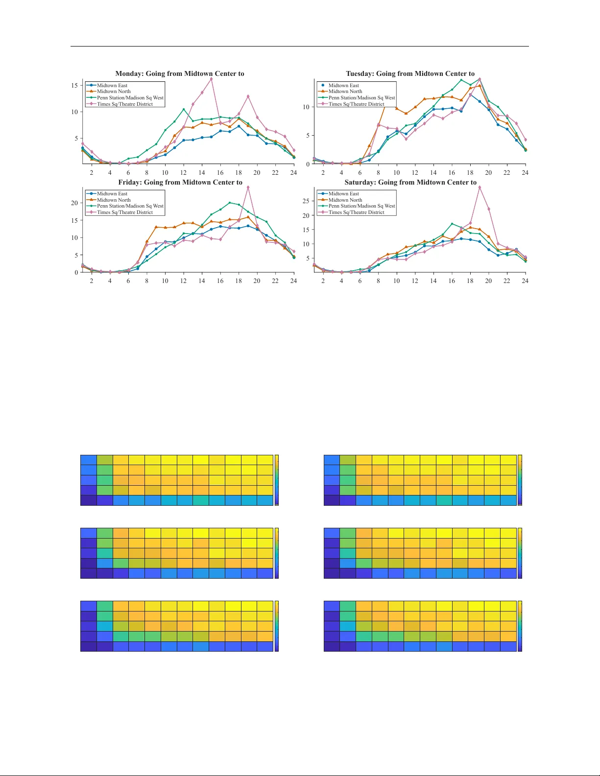
A D A P T I V E S U B S P A C E M O D E L I N G W I T H F U N C T I O N A L T U C K E R D E C O M P O S I T I O N P R E P R I N T Noah Steidle KU Leuven noahmaximilian.steidle@kuleuven.be Joppe De J onghe KU Leuven joppe.dejonghe@kuleuven.be Mariya Ishteva KU Leuven mariya.ishteva@kuleuven.be March 27, 2026 A B S T R AC T T ensors provide a structured representation for multidimensional data, yet discretization can obscure important information when such data originates from continuous processes. W e address this limitation by introducing a functional T ucker decomposition (FTD) that embeds mode-wise continuity constraints directly into the decomposition. The FTD emplo ys reproducing k ernel Hilbert spaces (RKHS) to model continuous modes without requiring an a-priori basis, while preserving the multi-linear subspace structure of the T ucker model. Through RKHS-driv en representation, the model yields adaptiv e and expressi ve factor descriptions that enable targeted modeling of subspaces. The value of this approach is demonstrated in domain-variant tensor classification. In particular , we illustrate its ef fectiveness with classification tasks in hyperspectral imaging and multiv ariate time-series analysis, highlighting the benefits of combining structural decomposition with functional adaptability . Keyw ords T ensor · T ucker decomposition · Reproducing kernel Hilbert space · Classification 1 Introduction T ensors and tensor decompositions have been used in a wide variety of applications to model high-dimensional discrete data or measurements, structured in a tabular scheme. Examples of tensor decompositions include the canonical polyadic decomposition (CPD) and T ucker decomposition (TD), which hav e been widely applied in signal processing, chemometrics and numerical analysis contexts [1]. As a method, tensor models process data entries in their discrete and tabular format. Howe ver , in practice, discrete data captured in the tensor may originate from a continuous system which moti vates the realization of a tensor with one or more continuous modes. Mathematically , this structure is called a quasitensor , generalizing the notion of quasimatrices [14]. Standard tensor decompositions such as CPD and TD do not take into account the continuity of quasitensors originating from smooth data processes, effecti vely losing this information. T o this end, sev eral publications hav e aimed at addressing the idea of functional modes in the context of the CPD and TD. For instance, the authors of [17] proposed to constrain the elements of the functional factor matrix to come from a smooth B-spline basis. Beylkin et al. [2] introduced a CPD model where all the modes are functional which corresponds to functional regression in three dimensions and is related to the work of Dolgov et al. [3] who apply the same idea to the TD with Chebyshev interpolation for the functional modes. Also, structured data fusion proposed in [13] provides a general optimization and modeling framework which includes mode-wise smoothness constraints via its factor-structure transformations. More recent examples include the work of T ang, Larsen, Han and K olda [15, 8, 4] which culminated in the CP- HiFi decomposition that allo ws arbitrary numbers of continuous modes with a k ernel-based functional representation. Adaptiv e subspace modeling with functional T ucker decomposition P R E P R I N T Moreov er, Qian et al. [10] approached a smooth T ucker tensor decomposition by adding temporal smoothing penalties to better model continuous measurements of blood pressure and heart rates. In this work we inv estigate a functional Tuck er decomposition (FTD), driv en by the theoretical foundation of qua- sitensors and RKHS. The aim of this decomposition is to extract subspace information in each mode while retaining continuity in a specified mode. Consequentially , the functional representation can be used for interpolation of the func- tional mode powered by the multi-linear structure of the input tensor . Furthermore, the model enables domain transfer in a classification conte xt, building upon the classification approach dri ven by the T ucker decomposition introduced in [11]. This is done by le veraging the functional representation, which allows to construct a tailored classification model at test time, incorporating a priori kno wledge about the functional mode, compared to a fixed model used during test- ing. Namely , the functional mode enables an adaptiv e change of sampling points which construct the model tensor during the testing phase. This allows the model to be tailored based on a priori knowledge of the test data without the need to specify and train a new model. Figure 1 illustrate the framework of adaptiv e subspace modeling based on the FTD. ( a ) ( b ) ( c ) Figure 1: Overview of the domain transfer framework driven by the functional Tuck er decomposition (FTD). (a) An input tensor X is interpreted as slices in the third mode corresponding to sampling points x 1 , x 2 , x 3 , and x 4 . (b) The FTD allows to describe the functional mode in terms of different sampling points e x 1 , e x 2 , e x 3 , and e x 4 . (c) The adapted sampling points e x 1 , e x 2 , e x 3 , and e x 4 allow to reconstruct the tensor X in a different domain, yielding a ne w tensor e X . In the follo wing, we outline notation and technical preliminaries, as well as the methodology of TD-based classification in Section 2. In a next step, the model and optimization formulation for the functional T ucker decomposition as well as an algorithmic strategy to solve the optimization problem is presented in Section 3. Finally , Section 4 provides experimental results with semi-synthetic data and two real-world datasets that showcase the benefits of combining structural decomposition with functional adaptability in the context of interpolation and classification. 2 Notation and preliminaries 2.1 T ensors and T uck er decomposition In the following, v ectors are denoted by bold lowercase Roman letters (e.g., a , b ), matrices by bold uppercase Roman letters (e.g., A , B ) and tensors by bold uppercase calligraphy letters (e.g., X , Y ). Following [1], a tensor X ∈ R m × n × p is said to be of or der ord ( X ) = 3 , referring to its number of dimensions, also known as ways or modes . The slices of X 2 Adaptiv e subspace modeling with functional T ucker decomposition P R E P R I N T are its 2 -w ay subtensors which can be obtained by fixing all b ut two indices of the tensor . For k ∈ [3] := { 1 , 2 , 3 } , the mode- k fibers of X are defined by the 1 -way subtensors obtained by fixing ev ery b ut the k th mode index. X ( k ) denotes the unfolding of X over its k th mode, as described in [7], i.e., the columns of a mode- k unfolding are the mode- k tensor fibers. The tensor-times-matrix pr oduct or k -mode pr oduct Y = X • k A defines a mode-wise multiplication of a tensor X with a matrix A via Y ( k ) = AX ( k ) , i.e., the matrix A is acting on the mode- k fiber of X . Let || · || denote the matrix Frobenius norm. Giv en a positive definite matrix K ∈ R p × p , define the weighted matrix norm via || W || 2 K = s X i =1 w T i Kw i = v ec( W )( I s ⊗ K ) v ec( W ) (1) for a matrix W ∈ R p × s . Furthermore, || X || describes the norm of X which equals the square root of the sum of all squared tensor entries, i.e., || X || = q P i P j P k x 2 ij k . It holds || X || = || X ( k ) || for each mode- k unfolding of X . Finally , ⊗ denotes the Kronecker product. The follo wing three properties from [1] of the Kronecker product will be helpful ( A ⊗ B ) T = A T ⊗ B T , (2) ( A ⊗ B ) ( C ⊗ D ) = ( AC ) ⊗ ( BD ) , (3) v ec  ACB T  = ( B ⊗ A ) vec( C ) . (4) Classical tabular tensors represent discrete measurements within their modes. Lifting this restriction to allow con- tinuous processes in part of the modes yields the concept of quasitensors which naturally generalize the notion of quasimatrices [14]. A quasimatrix e A ∈ R ∞× s describes an ordered set of s univ ariate functions defined on the same interval, e A = [ a 1 · · · a s ] where a γ : R → R for γ ∈ [ s ] . Ev aluating the quasimatrix e A on a set of p evaluation points I = { x 1 · · · x p } ⊂ R yields a (tab ular) matrix b A I ∈ R p × s as follows b A I =     a 1 ( x 1 ) a 2 ( x 1 ) · · · a s ( x 1 ) a 1 ( x 2 ) a 2 ( x 2 ) · · · a s ( x 2 ) . . . . . . . . . . . . a 1 ( x p ) a 2 ( x p ) · · · a s ( x p )     ∈ R p × s . An analogous approach expands the concept of quasimatrices to quasitensors e T ∈ R m × n ×∞ and their ev aluated counterpart b T I ∈ R m × n × p . In the following work, we consider quasitensors that consist of two discrete modes and one continuous mode. Nonetheless, the number of discrete modes can be expanded arbitrarily . W ithout loss of generality , the continuous mode of a tensor is assumed to correspond to the last dimension. Recent findings built upon the theoretical foundation of quasimatrices and quasitensor to dev elop decompositions of matrices and tensors which model continuous processes in at least one of their modes [17, 2, 3, 15, 8, 4, 10]. Similar to matrix decompositions such as the singular v alue decomposition (SVD), tensors can be decomposed. The rank- ( q , r , s ) T uck er decomposition aims to approximate a tensor X ∈ R m × n × p by a cor e tensor G ∈ R q × r × s and factor matrices A ∈ R m × q , B ∈ R n × r and C ∈ R p × s such that X ≈ G • 1 A • 2 B • 3 C (5) [5, 18]. An alternative way to express the T ucker formulation in eq. (5) is X ≈ [ [ G ; A , B , C ] ] . Gi ven an exact T ucker decomposition, i.e., X = [ [ G ; A , B , C ] ] , its unfoldings can be directly computed via X (1) = A G (1) ( C ⊗ B ) T = A ( G • 2 B • 3 C ) (1) ; (6) X (2) = B G (2) ( C ⊗ A ) T = B ( G • 1 A • 3 C ) (2) ; (7) X (3) = C G (3) ( B ⊗ A ) T = C ( G • 1 A • 2 B ) (3) . (8) From a computational perspective, the second formulation of eqs. (6) to (8) is usually more efficient as it sav es the computation of a Kronecker product. In general, solving the T ucker decomposition problem jointly for all factor matrices is challenging. Consequently , optimization formulations typically rely on alternating least-squares (ALS) methods that estimate one f actor matrix at a time through mode-wise optimization, followed by the computation of the core tensor in a final step. Algorithms based on this framework include the higher-order singular value decomposition (HOSVD), the sequentially truncated HOSVD (ST-HOSVD), and higher-order orthogonal iteration (HOOI) [1]. 3 Adaptiv e subspace modeling with functional T ucker decomposition P R E P R I N T 2.2 Classification using HOSVD The classification method considered in this work is a multidimensional variant of the Soft Independent Modeling by Class Analogy (SIMCA) algorithm [21], in its high-dimensional version initially presented by Sav as and Eld ´ en [11]. The approach follows the principle of class modeling (CM) by constructing a small set of basis arrays from the HOSVD of the tensor of stacked samples for each category with the aim of describing dominant properties. The algorithm operates in two steps: first, within the training stage, class models are constructed from the training data by truncation of the HOSVD of the tensor of stacked samples. Second, in the testing stage, a residual between an unknown input and each class model is computed and used to propose a class. Even though the seminal paper of this method did not consider the optimization of model parameters or the validation of the model in separate steps, it is noted that a full implementation of class modeling by means of SIMCA includes both these important steps. Further information on model parameter optimization and model validation within the SIMCA re gime can be found in [20]. T raining stage Let C denote the number of classes. W ithout loss of generality , assume that each sample is of the form X ∈ R n × p . The first step of the method works on training data which consists of all training samples of a class µ ∈ [ C ] stacked along the first mode, yielding the tensor X µ training ∈ R M µ × n × p , where M µ is the number of training samples for class µ and n × p is the size of each training sample. A rank-( M µ , r , s ) T ucker decomposition of X µ training is computed via the HOSVD as X µ training ≈ G µ • 1 A µ • 2 B µ • 3 C µ for r ≤ n and s ≤ p . Then, by setting D µ = G µ • 2 B µ • 3 C µ and D µ ν = D µ ( ν, : , :) for all ν ∈ [ M µ ] , it holds X µ training ≈ D µ • 1 A µ and the matrices { D µ 1 , . . . , D µ k } span a small and dominant subspace that characterizes class µ for a truncation param- eter k < M µ . In other words, the basis for class µ is gi ven by T µ = ( D µ ν ) k ν =1 where each D µ ν is normalized. Here, we note that the computation via the HOSVD guarantees orthogonality of D µ ν for all ν and µ due to the all-orthogonality of the core G µ ; this will prove helpful in the test stage. Finally , this process is repeated for all classes µ 1 , . . . , µ C , yielding the corresponding class-wise bases T µ 1 , . . . , T µ C . T est stage Let Y ∈ R n × p be a normalized test sample without a class label. In order to assign it to a class, the goal is to find the basis which provides the best approximation of Y . This translates to the minimization problems min α µ 1 ,...,α µ k || Y − k X ν =1 α µ ν D µ ν || with unkno wns α µ 1 , . . . , α µ k . Owing to the orthonormality of D µ ν the solution is given by b α µ ν = ⟨ Y , D µ ν ⟩ . As a result, the residual can be computed via R ( µ ) = || Y − k X ν =1 b α µ ν D µ ν || 2 = 1 − k X ν =1 ⟨ Y , D µ ν ⟩ 2 according to the orthonormality of D µ ν for all ν ∈ [ k ] [11]. At last, the test sample Y ∈ R n × p is assigned to the class µ ∗ where R ( µ ∗ ) is minimal. 2.3 Reproducing k ernel Hilbert spaces (RKHS) For the purpose of modeling the functional mode in the T ucker decomposition, the functions are chosen from a r epro- ducing kernel Hilbert space (RKHS). A RKHS is a Hilbert space of functions with useful representation properties through the notion of a kernel. More precisely , for a non-empty set I = { x 1 , . . . , x p } with x i ∈ R for all i ∈ [ p ] , let K : I × I → R be a symmetric positi ve semidefinite (psd) kernel function with corresponding kernel matrix K defined by its elements K ij = K ( x i , x j ) . A prominent example is the Gaussian kernel which is defined via K ( x i , x j ) = exp  − ( x i − x j ) 2 2 c 2  4 Adaptiv e subspace modeling with functional T ucker decomposition P R E P R I N T for a parameter c  = 0 . In the following, functions f and g are constructed via f ( · ) = p X i =1 α i K ( · , x i ) and g ( · ) = p X j =1 β j K ( · , x j ) for α i , β j ∈ R and x i , x j ∈ I for i, j ∈ [ p ] . This leads to the natural definition of a dot product by ⟨ f , g ⟩ K = P p i,j =1 α i β j K ( x i , x j ) and, accordingly , the induced norm || f || K := p ⟨ f , f ⟩ K . Now , the space of linear combinations of the kernel which is completed with respect to || f || K , i.e., H K := span {K ( · , x i ) | x i ∈ I } , is called a reproducing kernel Hilbert space (RKHS). The important r epr oducing kernel pr operty states that ⟨K ( · , x i ) , f ⟩ K = f ( x i ) for x i ∈ I . This means that a function f at a point x i can be ev aluated by taking an inner product with the ev aluated kernel K ( · , x i ) [12]. Furthermore, theorem 1 displays the Repr esenter theorem which states that a large subset of infinite dimensional optimization problems ov er H K admits solutions in terms of linear combinations of the kernel ev aluated on a finite set of particular design points {K ( · , x 1 ) , . . . , K ( · , x p ) } . Theorem 1 (Repr esenter theorem [12]) Denote by Ω : [0 , ∞ ) → R a strictly monotonic increasing function, by I = { x 1 , . . . , x p } a set, and by c : ( I × R 2 ) p → R ∪ {∞} an arbitrary loss function. Then each minimizer f ∗ ∈ H K of the r e gularized risk c (( x 1 , y 1 , f ∗ ( x 1 )) , . . . , ( x p , y p , f ∗ ( x p ))) + Ω( || f ∗ || K ) admits a r epresentation of the form f ∗ ( · ) = p X i =1 w i K ( · , x i ) . In the following, analogous to [15], we only consider the important variant of theorem 1, originally stated by [6], focusing on the point-wise mean squared loss c (( x 1 , y 1 , f ( x 1 )) , . . . , ( x p , y p , f ( x p ))) = 1 p p X i =1 ( y i − f ( x i )) 2 and Ω( || f || K ) = λ 2 || f || 2 K for λ > 0 . This setup guarantees an accessible solution of the form f ∗ ( · ) = p X i =1 w i K ( · , x i ) = b K w , for some w ∈ R p and a quasimatrix b K = K ( · , x ) ∈ R ∞× p for x = [ x 1 x 2 . . . x p ] T which - ev aluated at the design points in I - corresponds to the kernel matrix K ∈ R p × p . This representation will prove fa vorable to the optimization problem in Section 3. 3 Functional T ucker decomposition In this section we derive a Functional T ucker decomposition (FTD) by employing the theory of reproducing kernel Hilbert spaces (RKHS). T o this end, we first incorporate the RKHS formulation into the T ucker model by adjusting the corresponding optimization problem in Section 3.1. In Section 3.2, we deriv e closed form solutions for each variable of the optimization problem individually . Finally , the solutions are merged into the algorithmic formulation in Section 3.2.3. It is noted that the following deriv ation is based on input tensors with two discrete modes and one continuous mode. Nonetheless, the theory can be generalized to arbitrary numbers of discrete modes thanks to the mode-wise perspectiv e of the optimization problem. 5 Adaptiv e subspace modeling with functional T ucker decomposition P R E P R I N T 3.1 Setup Let m, n, p, q , r ∈ N with q ≤ m and r ≤ n and I ⊂ R . Finding a functional rank-( q , r , s ) T ucker decomposition, translates to decomposing a quasitensor e T ∈ R m × n ×∞ as e T = [ [ G ; A , B , e C ] ] (9) for a core tensor G ∈ R q × r × p , factor matrices A = [ a 1 · · · a q ] ∈ R m × q and B = [ b 1 · · · b r ] ∈ R n × r , as well as a quasimatrix e C ∈ R ∞× s . In practice, a tensor like above is considered for a discrete set of measurements in the continuous mode which yields a discrete tabular tensor . Therefore, define the tensor b T I ∈ R m × n × p as the quasitensor e T e valuated at a set of p design points I = { x 1 , . . . , x p } ⊂ R in the third mode. This yields a classical rank-( q , r , s ) T ucker decomposition by ev aluating eq. (9) according to b T I = [ [ G ; A , B , b C I ] ] , where b C I ∈ R p × s is the quasimatrix ev aluated at the design points in I , i.e., b C I =     c 1 ( x 1 ) c 2 ( x 1 ) · · · c s ( x 1 ) c 1 ( x 2 ) c 2 ( x 2 ) · · · c s ( x 2 ) . . . . . . . . . . . . c 1 ( x p ) c 2 ( x p ) · · · c s ( x p )     . Introducing the RKHS methodology outlined in Section 2.3, the functions c γ in e C = [ c 1 · · · c s ] for γ ∈ [ s ] are chosen from a RKHS with kernel function K : I × I → R where I = { x 1 , . . . , x p } ⊂ R ; this yields a kernel matrix K ∈ R p × p . Then, for the corresponding weight matrix W ∈ R p × s , the functions c γ are described via c γ ( · ) = p X k =1 w kγ K ( · , x k ) , or c C I = KW according to the Representer Theorem described in theorem 1. As a result, for an e valuated input tensor b T I , this yields the optimization problem min G , A , B , W 1 2 || b T I − G • 1 A • 2 B • 3 KW || 2 + λ || W || 2 K , (10) for G ∈ R q × r × s , A ∈ R m × q , B ∈ R n × r , W ∈ R p × s and a regularization parameter λ > 0 . Hereby , the re gularization term stems from the Representer Theorem in Section 2.3. In the following, for fixed I = { x 1 , . . . , x p } , we will denote b T I by b T . 3.2 Optimization problem The following section outlines how to solve the optimization problem eq. (10) independently for factor matrices of discrete modes A and B , the weight matrix W and the core tensor G . In addition to the mathematical solution, we outline algorithmic details to illustrate how the procedure is carried out in practice. 3.2.1 Solution for discr ete modes W ithout loss of generality , the goal is to find a solution to min A 1 2 || b T − G • 1 A • 2 B • 3 KW || 2 (11) for all other variables fix ed. By mode- 1 unfolding, the solution to the problem is described via b T (1) = A ( G • 2 B • 3 KW ) (1) , according to eq. (6). This formulation is computationally more efficient because it avoids explicitly forming the Kronecker product. Analogously , for B it follo ws from eq. (7) that b T (2) = B ( G • 1 A • 3 KW ) (2) . After solving the linear system, the solution is orthogonalized; for instance, by employing a SVD. In this case, the factor matrices A and B are replaced by their left leading singular vectors, while the remaining components of the de- composition are absorbed into the core tensor . Consequently , the factor matrices A and B can be treated as orthogonal in the subsequent steps. 6 Adaptiv e subspace modeling with functional T ucker decomposition P R E P R I N T 3.2.2 Solution for continuous mode The goal is to find a solution to min W 1 2 || b T − G • 1 A • 2 B • 3 KW || 2 + λ || W || 2 K sub j . to W ∈ R p × s for λ > 0 . After extracting the objecti ve function and writing it as F : R p × s → R dependent on W F ( W ) = 1 2 || b T − G • 1 A • 2 B • 3 KW || 2 + λ || W || 2 K the first part can be unfolded with respect to the third mode and rewritten according to 1 2 || b T (3) − KWG (3) ( B ⊗ A ) T || 2 F = 1 2 || vec( b T (3) ) − vec( KWG (3) ( B ⊗ A ) T ) || 2 2 = 1 2 || vec( b T (3) ) − (( B ⊗ A ) G T (3) ⊗ K ) v ec( W ) || 2 2 , by employing eqs. (4) and (8), while without loss of generalization the regularization part can be reformulated via λ 2 || W || 2 K = λ 2 v ec ( W ) T ( I s ⊗ K ) v ec( W ) by using eq. (1). Computing the gradient of F with respect to vec( W ) yields [( B ⊗ A ) G T (3) ⊗ K ] T [v ec( b T (3) ) − ((( B ⊗ A ) G T (3) ⊗ K ) v ec( W ))] + λ ( I s ⊗ K ) v ec( W ) which, by factoring out v ec( W ) and setting it equal to 0 returns [(( B ⊗ A ) G T (3) ⊗ K ) T (( B ⊗ A ) G T (3) ⊗ K ) + λ ( I s ⊗ K )] v ec( W ) = [( B ⊗ A ) G T (3) ⊗ K ] T v ec( b T (3) ) By properties eq. (2) and eq. (3) of the Kronecker product, this is equi valent to [( G (3) ( B ⊗ A ) T ( B ⊗ A ) G T (3) ) ⊗ K 2 + λ ( I s ⊗ K )] v ec( W ) = [ G (3) ( B ⊗ A ) T ⊗ K ] v ec( b T (3) ) Then I s ⊗ K can be factored out according to ( I s ⊗ K )( G (3) ( B T B ⊗ A T A ) G (3) T ⊗ K + λI sp ) vec( W ) = ( I s ⊗ K )[ G (3) ( B ⊗ A ) T ⊗ I p ] vec( b T (3) ) which, assuming K is full rank, leads to ( G (3) G T (3) ⊗ K + λI sp ) vec( W ) = v ec( b T (3) ( B ⊗ A ) G T (3) ) due to the orthogonality of A and B and Equation (4). Again, the right hand side with the Kronecker product can be rewritten in terms of v ec(( b T • 1 A T • 2 B T ) (3) G T (3) ) and the resulting linear system is solved for W . Solution for cor e tensor The goal is to find a solution to min G 1 2 || b T − G • 1 A • 2 B • 3 KW || 2 sub j . to G ∈ R q × r × s for all other variables fix ed. In vectorized form, this is equi valent to the linear least squares problem min G 1 2 || vec( b T ) − ( KW ⊗ B ⊗ A ) vec( G ) || 2 2 sub j . to G ∈ R q × r × s with yields the system of linear equations ( KW ⊗ B ⊗ A ) vec( G ) = vec( b T ) . Howe ver , computing the Kronecker product KW ⊗ B ⊗ A might be computationally infeasible for matrices of larger size due to the amount of memory needed. 7 Adaptiv e subspace modeling with functional T ucker decomposition P R E P R I N T Therefore, in the algorithm, we use an alternative strategy to avoid the Kronecker product by exploiting the non- uniqueness of the T ucker decomposition. It holds that any T ucker decomposition with truncated core tensor , i.e., q < m , r < n and s < p , can be reformulated as a T ucker decomposition with orthogonal factors [1, 5.4]. For this reason, we orthogonalize the factor matrices of the discrete modes A and B and update the core tensor G accordingly after every update of the factors. This approach has already been described in the solution for discrete modes in Section 3.2.1. Turning to the factor matrix of the continuous mode C = KW , this approach would not work as the functional model is not in variant to orthogonalization. Nonetheless, the orthogonal factor matrices A and B can be used to update the core tensor in the first and second mode via Y = b T • 1 A T • 2 B T , before the final core tensor in matrix format is obtained by solving the linear system CG (3) = Y (3) where Y (3) is the 3 -mode unfolding of Y . 3.2.3 Algorithm A pseudo implementation for the computation of the functional T ucker decomposition for a 3 -way tensor with two tabular dimensions and continuous third mode is depicted in Algorithm 1. The orthogonalization step explained in Sections 3.2.1 and 3.2.2 is based on the SVD. For instance, the factor matrix A is decomposed according to A = U 1 Σ 1 V T 1 . Then, the factor matrix is updated to be U 1 while Σ 1 V T 1 is pushed to the core, i.e., G ← G • 1 (Σ 1 ∗ V T 1 ) . The same holds for B . Furthermore, the placeholder function RESHAPE reshapes vectors to matrices and matrices to tensors according to the inserted dimensions. Finally , a break condition is b uilt into the algorithm based on the change of the relati ve approximation error | ϵ t − ϵ t − 1 | between iterations t − 1 and t . If the change is smaller than a pre-defined threshold τ multiplied by the norm of the input tensor, the algorithm is concluded. 4 Experimental results In this section, we demonstrate the capabilities of adapti ve subspace modeling with the functional Tuck er decompo- sition through three experiments. First, a semi-synthetic dataset, built on the traditional task of digit classification, is considered, while the second and third experiment turn to real-world data in the realm of classification of multi- variate time-series and hyperspectral images. By stacking samples in an additional mode, all three examples inv olve 4 -way tensors. Since the datasets contain only one continuous mode (with the remaining modes being discrete), the theoretical framew ork presented above remains applicable. 4.1 Semi-synthetic data 4.1.1 Dataset The first experiment examines a semi-synthetic dataset which builds upon the US postal service (USPS) database [9]. The USPS dataset consists of 16 × 16 images of digits from 0 to 9 stemming from ZIP code scans of US Postal mail en velopes and - among others - was used to sho wcase the classification with the HOSVD in [11]. By introducing an additional mode based on continuous functions, we can le verage adaptiv e subspace modeling within the FTD and analyze the adapted digit classification problem in this extended setting. T o this end, each digit is split into two parts. These sub-parts are then individually multiplied via an outer product with class-specific function ev aluations and recombined afterw ards. The process of expanding a digit by a continuous mode is illustrated in fig. 2. From a technical perspectiv e, the functions associated with class c are represented by two e valuation v ectors s c, upper ∈ R p and s c, lower ∈ R p . For a sample Y c ∈ R 16 × 16 of class c , the tensorized sample Y c ∈ R 16 × 16 × p is constructed as Y c = Y lower c ◦ s c, lower + Y upper c ◦ s c, upper . Here, Y lower c denotes the sample with its upper half set to zero, while Y upper c corresponds to the image with its lower half set to zero. By choosing the vectors s c, lower and s c, upper to be linearly independent, the mode- 3 rank of Y c is guaranteed to be 2 . Repeating this process for all samples of a certain digit class c ∈ { 0 , 1 , . . . , 9 } , the final class objects are obtained by stacking samples of the same class in the first mode, yielding a tensor X c ∈ R N c × 16 × 16 × p . Here, N c denotes the number of samples for the respectiv e class. W e construct s c, lower and s s c, upper by fitting smoothing 8 Adaptiv e subspace modeling with functional T ucker decomposition P R E P R I N T Algorithm 1 Functional T ucker decomposition for 3 -way tensor with continuous third mode Input: T ∈ R m × n × p , K ∈ R p × p , M A X I T E R S ∈ N , τ ∈ R + Output: { G , A , B , W } such that T ≈ G • 1 A • 2 B • 3 KW 1: Initialize A ∈ R m × q , B ∈ R n × r , W ∈ R p × s , G ∈ R q × r × s 2: T ← || T || 3: C ← KW 4: f or t = 1 , 2 , . . . , M A X I T E R S do 5: 6: A 1 ← Solution of A 1  G (1) ( C ⊗ B ) T  = T (1) 7: [ U 1 , Σ 1 , V 1 ] ← SVD ( A 1 , q ) 8: A ← U 1 Update 1st discrete factor matrix 9: G ← G • 1 (Σ 1 V T 1 ) Update core tensor 10: 11: B 1 ← Solution of  G (2) ( C ⊗ A ) T  = T (2) 12: [ U 2 , Σ 2 , V 2 ] ← SVD ( B 1 , r ) 13: B ← U 2 Update 2nd discrete factor matrix 14: G ← G • 2 (Σ 2 V T 2 ) Update core tensor 15: 16: L ← G (3) G T (3) ⊗ K + λI sp 17: R ← vec( T (3) ( B ⊗ A ) G T (3) ) 18: W v ec ← Solution of LW v ec = R 19: W ← RESHAPE ( W v ec , [ p s ]) 20: C ← KW Update continuous factor matrix 21: Y ← T • 1 A T • 2 B T 22: G (3) ← Solution of CG (3) = Y (3) 23: G ← RESHAPE ( G (3) , [ q r s ]) Update core tensor 24: 25: ϵ t ← || T − G • 1 A • 2 B • 3 C || / T Check stop condition 26: if t > 1 and | ϵ t − ϵ t − 1 | < τ T then 27: break 28: end if 29: 30: end f or 31: r eturn { G , A , B , W } splines to 10 uniform random samples from (1 , 10) and e valuating them at p = 50 points. In general, 85% of the data is used for training while the remaining 15% are reserv ed for testing. In the following, we will use the semi-synthetic digit dataset to illustrate the classification in the context of a changed domain after training. T o this end, tw o dif ferent sampling domains are considered in training and test. Finally , the goal is to bridge both steps by application of adaptiv e subspace modeling with the FTD. W ith the purpose of representing two dif ferent domains for training and test, the av ailable set of p sampling points is split. Specifically , the training is based on every fourth sampling point in the continuous mode, i.e., the training employs the tensor built of slices X c (: , : , : , i ) for i ∈ { 1 , 5 , 9 , . . . , 45 , 49 } . Then, the computation of the FTD, based on this reduced domain, enables the interpolation of missing sampling points by definition of an alternati ve kernel according to the complete set of p = 50 sampling points. For illustration purposes, the reconstruction of X 5 (1 , 5 , 5 , :) , i.e., the continuous mode of X for the first sample of class 5 and the pixel at position (5 , 5) , is displayed in fig. 3. In particular , the reconstruction is compared for Gaussian kernel parameters d ∈ { 1 , 2 , 3 , 4 } . It is noted that the selection of the Gaussian kernel parameter is relev ant for achieving an accurate reconstruction. Furthermore, although the reconstructed curves provide a satisfactory approximation of the true function for suitable d , it is noted, that the distribution of sampling points inherently limits the best possible approximation. 9 Adaptiv e subspace modeling with functional T ucker decomposition P R E P R I N T c u t Figure 2: Illustration of e xpanding a digit sample by an additional mode based on two independent smoothing splines. 0 0.1 0.2 0.3 0.4 0.5 0.6 0.7 0.8 0.9 1 1 2 3 4 5 6 7 8 d=1 Original Reconstruction 0 0.1 0.2 0.3 0.4 0.5 0.6 0.7 0.8 0.9 1 2 3 4 5 6 7 8 d=2 Original Reconstruction 0 0.1 0.2 0.3 0.4 0.5 0.6 0.7 0.8 0.9 1 2 3 4 5 6 7 8 d=3 Original Reconstruction 0 0.1 0.2 0.3 0.4 0.5 0.6 0.7 0.8 0.9 1 2 3 4 5 6 7 8 d=4 Original Reconstruction Figure 3: Original and reconstruction of X 5 (1 , 5 , 5 , :) . 10 Adaptiv e subspace modeling with functional T ucker decomposition P R E P R I N T 4.1.2 Classification After having illustrated the interpolation capacity of the FTD, the functional approximation is used for classification in the context of a domain transfer . As before, the training data is constructed by restricting the sampling points to e very fourth index, before the FTD yields a corresponding factorization. In a next step, the goal is to run the classification on data with a dif ferent sampling domain. Therefore, the test data is adjusted to only contain ev ery av ailable sample point between indices 1 and 13 ; this necessitates a domain transfer . By employing the same number of sample points for training and test, we make sure the FTD can be compared to the HOSVD. In order to incorporate the domain transfer , after obtaining the functional Tuck er decomposition, the reconstruction of the class tensor is computed by employing the alternativ e kernel with corresponding domain, i.e., the set of sample points between indices 1 and 13 . This yields a reconstruction of the class tensor in the ne w domain. Then, the HOSVD of the reconstruction enables the HOSVD-driv en classification approach described in Section 2.2. This approach is repeated for all classes and, finally , an unknown sample can be classified by comparing it to all av ailable bases and choosing the best according to the lowest residual. The algorithm is run with Gaussian kernel parameter d = 4 . The truncation parameters are set to 5 in the spatial mode and 2 in the continuous mode, according to existing knowledge from [11] and construction of the continuous mode. Finally , figs. 4 and 5 illustrate the results with and without the adaptiv e subspace modeling by the FTD model. In particular , fig. 4 indicates the success rates for different choices of truncation in the sample mode, while fig. 5 focuses on the macro F1 score for a more balanced perspectiv e on the multi-class dataset. Indi vidually , the figures compare the corresponding metrics with equal sets of sampling points for training and test on the left hand side, while the right hand side is based on different training and test domains. While equal sampling points used in training and test yield similar classification results for the HOSVD and FTD, different sampling points necessitate a domain transfer , as can be seen by the decay in classification po wer of the HOSVD and comparable accuracy of the FTD. k 1 2 3 4 5 6 7 8 9 10 Success rate 0.8 0.85 0.9 0.95 1 Equal training and test domains HOSVD (trained and tested on indices 1:4:50) FTD (trained and tested on indices 1:4:50) k 1 2 3 4 5 6 7 8 9 10 Success rate 0.8 0.85 0.9 0.95 1 Differ ent training and test domains HOSVD (trained on indices 1:4:50, tested on indices 1:1:13) FTD (trained on indices 1:4:50, transferred to 1:1:13) Figure 4: Success rates of HOSVD- and FTD-driven classification for equal (l.h.s.) and dif ferent (r .h.s.) training and test domains for the semi-synthetic digit data. While the FTD and the HOSVD achie ve comparable performance when the sampling points during training and test match, a noticeable performance gap emerges when dif ferent sampling points are used. 4.2 Multivariate time-series data: T rip records of NYC taxis in 2024 4.2.1 Dataset Since 2009, the NYC T axi and Limousine Commission (TLC) provides monthly taxi trip records capturing various fields such as pickup and drop-off dates, times and locations [16]. The following analysis considers NYC taxi trip 11 Adaptiv e subspace modeling with functional T ucker decomposition P R E P R I N T k 1 2 3 4 5 6 7 8 9 10 Macro F1 Score 0.8 0.85 0.9 0.95 1 k 1 2 3 4 5 6 7 8 9 10 Macro F1 Score 0.8 0.85 0.9 0.95 1 Equal training and test domains Differ ent training and test domains HOSVD (trained and tested on indices 1:4:50) FTD (trained and tested on indices 1:4:50) HOSVD (trained on indices 1:4:50, tested on indices 1:1:13) FTD (trained on indices 1:4:50, transferred to 1:1:13) Figure 5: Macro F1 scores of HOSVD- and FTD-driv en classification for equal (l.h.s.) and different (r .h.s.) training and test domains for the semi-synthetic digit data. As with the classification accuracy , the FTD and HOSVD perform similarly when training and test use identical sampling points. When the sampling points dif fer , howe ver , the adaptiv e subspace modeling allows the FTD to adapt accordingly . records from 2024, restraining the dataset to relev ant trips that either begin or end at one of the locations listed in table 1. The data is aggregated to hourly counts of trip records between two locations, split by day of the week. Hence, T able 1: Relev ant subset of NYC taxi pickup and drop-off locations. Index Zone Location ID 1 Midtown Center 161 2 Midtown East 162 3 Midtown North 163 4 Penn Station/Madison Sq W est 186 5 T imes Sq/Theatre District 230 for each class c ∈ { Monday , T uesday , . . . , Sunday } , a 4 -way tensor X c ∈ R N c × 5 × 5 × 24 cov ering 5 pickup and drop- off locations over 24 hours is considered. Hereby , the number of samples in class c is denoted by N c . For instance, the measurement X T uesday (4 , 2 , 3 , 9) = 5 indicates that 5 trips were recorded from Midtown East to Midtown North on the fourth T uesday of 2024 between 8am and 9am. For illustration purposes, fig. 6 presents yearly av erages per time of the day for Monday , T uesday , Friday and Saturday going from Midtown Center (Location ID 161 ) to the other locations. In a consistent approach to the previous experiment, the goal is to run the classification with a change of sampling points. Hence, the training data is based on e very second sampling point in the continuous mode, i.e., the training uses the tensor built of slices X c (: , : , : , i ) for i ∈ { 1 , 3 , 5 , . . . , 21 , 23 } . The goal is to run the classification on a different set of design points to illustrate the adaptive subspace modeling. In this case, the domain for testing is set to be every hour between 8 and 19 . 4.2.2 Classification Before the domain transfer , in a first step, the ov erall number of N = 348 samples is partitioned into subsets for training + validation ( 85% ) and test ( 15% ). Without existing knowledge of the dataset, 5 -fold cross validation is ex ecuted on the training + validation data to determine optimal ranks for the classification. Hereby , the validation runs the classification based on the HOSVD as explained in Section 2.2 and the resulting classification accuracies are determined for dif ferent combinations of truncation in the sample mode, in the modes for pickup and drop-of f locations 12 Adaptiv e subspace modeling with functional T ucker decomposition P R E P R I N T 2 4 6 8 10 12 14 16 18 20 22 24 5 10 15 Monday: Going fr om Midtown Center to Midtown East Midtown North Penn Station/Madison Sq W est T imes Sq/Theatre District 2 4 6 8 10 12 14 16 18 20 22 24 0 5 10 T uesday: Going fr om Midtown Center to Midtown East Midtown North Penn Station/Madison Sq W est T imes Sq/Theatre District 2 4 6 8 10 12 14 16 18 20 22 24 0 5 10 15 20 Friday: Going fr om Midtown Center to Midtown East Midtown North Penn Station/Madison Sq W est T imes Sq/Theatre District 2 4 6 8 10 12 14 16 18 20 22 24 5 10 15 20 25 Saturday: Going fr om Midtown Center to Midtown East Midtown North Penn Station/Madison Sq W est T imes Sq/Theatre District Figure 6: Y early av erage of NYC taxi trip records per time of the day going from Midtown Center (Location ID 161 ) to Midtown East (Location ID 162 ), Midtown North (Location ID 163 ), Penn Station/Madison Sq W est (Location ID 186 ) and T imes Sq/Theatre District (Location ID 230 ) on Mondays, T uesdays, Fridays and Saturdays. and the time mode. Here, HOSVD is employed instead of FTD to ensure that the f actorization remains independent of the specific domain transfer under consideration. Resulting heatmaps are displayed in fig. 7. While the results indicate symmetry in the ranks for pickup and drop-off locations, a rank greater than 1 is suggested by the v alidation results for both. Furthermore, depending on the truncation in the sample mode, the optimal hour rank gro ws in magnitude from 5 to 10 . W e note that these ranks are considered optimal by validation according to the HOSVD. Y et, the HOSVD does not consider the smoothness constraint, implying that optimal ranks for adaptive subspace modeling may be slightly larger . 1 2 3 4 5 6 7 8 9 1 0 1 1 12 HourRank 5 4 3 2 1 Startlocatio nRank k=5 0.2 0.3 0.4 0.5 0.6 0.7 1 2 3 4 5 6 7 8 9 1 0 1 1 12 HourRank 5 4 3 2 1 Endloca tionRank k=5 0.2 0.3 0.4 0.5 0.6 0.7 1 2 3 4 5 6 7 8 9 1 0 1 1 12 HourRank 5 4 3 2 1 Startlocatio nRank k=10 0.2 0.3 0.4 0.5 0.6 0.7 1 2 3 4 5 6 7 8 9 1 0 1 1 12 HourRank 5 4 3 2 1 Endloca tionRank k=10 0.2 0.3 0.4 0.5 0.6 0.7 1 2 3 4 5 6 7 8 9 1 0 1 1 12 HourRank 5 4 3 2 1 Startlocatio nRank k=15 0.2 0.3 0.4 0.5 0.6 0.7 1 2 3 4 5 6 7 8 9 1 0 1 1 12 HourRank 5 4 3 2 1 Endloca tionRank k=15 0.2 0.3 0.4 0.5 0.6 0.7 Figure 7: Results of 5 -fold cross validation in terms of HOSVD classification accuracy for different combinations of truncation in the sample mode (denoted by k ), in the modes for pickup and drop-off locations and the time mode. 13 Adaptiv e subspace modeling with functional T ucker decomposition P R E P R I N T The resulting classification accuracies and macro F1 scores on the test dataset are displayed in figs. 8 and 9. As before, after training the model on e very second av ailable sampling point the results are inferred on dif ferent sampling points. In this case, the considered slices are all indices between 8 and 19 . Furthermore, as suggested by the validation, the hour rank was set to 10 while the truncation for both the pickup and drop-off locations is symmetrically defined to be 4 . The Gaussian kernel is employed with parameter d = 1 . k 5 10 15 20 25 30 Success rate 0 0.1 0.2 0.3 0.4 0.5 0.6 0.7 0.8 0.9 1 k 5 10 15 20 25 30 Success rate 0 0.1 0.2 0.3 0.4 0.5 0.6 0.7 0.8 0.9 1 Equal training and test domains Differ ent training and test domains HOSVD (trained and tested on indices 1:2:24) FTD (trained and tested on indices 1:2:24) HOSVD (trained on indices 1:2:24, tested on indices 8:1:19) FTD (trained on indices 1:2:24, transferred to 8:1:19) Figure 8: Success rates of HOSVD- and FTD-dri ven classification for equal (l.h.s.) and different (r .h.s.) training and test domains for the NYC taxi trip data. On the left-hand side, classification accuracies of the FTD and the HOSVD-based model are similar , both lying around 0 . 7 . On the right-hand side, howe ver , a clear gap emerges due to the domain transfer: while the FTD still achiev es an accuracy of approximately 0 . 7 , the HOSVD-based classification drops to about 0 . 3 . Both the results in terms of the classification accuracy , as well as the macro F1 score indicate a successful transfer of the domain when comparing the metrics of the HOSVD and the FTD on the right-hand side of the figures. The variation of the results between the HOSVD and FTD in the context of equal training and test domains might be an artifact of the smaller sample size in combination with the random initialization of the computations. 4.3 Hyperspectral image data: Hyperspectral images of mangos 4.3.1 Dataset In this final study , we address the classification of close-range hyperspectral image (HSI) data under a domain transfer scenario. Here, the change of domain is represented by different wav elengths present in the data. The overall dataset consists of hyperspectral images of mangos cate gorized into three ripeness classes: UNRIPE , RIPE and O VERRIPE [19]. Images were recorded using a Specim FX 10 camera, resulting in 224 channels in a spectral range from 400 to 1000 nm and a spatial dimension of 64 × 64 . Moreover , the dataset consists of 121 samples in total which splits up into 39 , 52 and 30 instances of classes UNRIPE , RIPE and O VERRIPE , respectively . As before, the goal is to run the classification with a change of domain. Therefore, let the training domain be defined by ev ery fourth av ailable sampling value in the spectral mode, while the classification results are inferred on data consisting of every sampling value between indices 100 and 155 which translates to the spectral range from 604 . 9250 to 714 . 3090 nm. 4.3.2 Classification T runcation parameters were determined by stratified 5 -fold cross-validation comparing the classification accuracies yielded by the HOSVD-based classification approach. In particular , the truncation in the sample mode, the spatial mode and the spectral mode was tested on 85% of all av ailable samples. Hereby , due to a symmetry argument, the spatial rank was set equal for both spatial dimensions. T wo heatmaps displaying the results for truncations in the 14 Adaptiv e subspace modeling with functional T ucker decomposition P R E P R I N T k 5 10 15 20 25 30 Macro F1 Score 0 0.1 0.2 0.3 0.4 0.5 0.6 0.7 0.8 0.9 1 k 5 10 15 20 25 30 Macro F1 Score 0 0.1 0.2 0.3 0.4 0.5 0.6 0.7 0.8 0.9 1 Equal training and test domains Differ ent training and test domains HOSVD (trained and tested on indices 1:2:24) FTD (trained and tested on indices 1:2:24) HOSVD (trained on indices 1:2:24, tested on indices 8:1:19) FTD (trained on indices 1:2:24, transferred to 8:1:19) Figure 9: Macro F1 scores of HOSVD- and FTD-driv en classification for equal (l.h.s.) and different (r .h.s.) training and test domains for the NYC taxi trip data. The Macro F1 scores confirm the discriminativ e po wer observed in the domain-transfer setting, consistent with the findings from the classification accuracy . When the training and test sampling domains coincide, both the FTD and the HOSVD perform similarly . In contrast, under domain transfer, the HOSVD scores drop to approximately 0 . 3 , whereas the FTD maintains a stable Macro F1 score of around 0 . 7 as before. sample mode at k = 5 and k = 10 are displayed in fig. 10. The v alidation suggests the optimal spatial rank higher than the spectral rank. As a result, for testing, a spatial rank of 18 and a spectral rank of 6 were considered. Based on the parameters identified in the validation step, the results on the remaining test data are given in terms of the classification accuracy in fig. 11 and macro F1 scores in fig. 12, respectively . As before, the left-side of the charts considers the equal domain in training as in testing, while the right hand-side inv estigates the domain transfer for the FTD. The left-hand panels of both charts fig. 11 and fig. 12 illustrate the consistent performance of HOSVD and FTD under identical training conditions. In contrast, the right-hand panels illustrate the effect of the adaptive subspace modeling on the classification results. While the success rates of the HOSVD-based classification do not exceed the 40% threshold - which corresponds to always predicting RIPE in the classification process - the continuous FTD model achie ves a classification accurac y of more than 60% for k = 10 . Figure 12 supports this finding by considering the macro F1 score, which compensates for class imbalance by weighting all classes equally . Consequently , the performance gap between HOSVD and FTD becomes e ven more pronounced in this figure. 5 Conclusions In this paper , we proposed a functional T ucker decomposition (FTD) which models continuity in one tensor mode using the flexible representation capabilities of reproducing kernel Hilbert spaces (RKHS). Building on this concept, we dev eloped an adaptive subspace modeling framew ork that supports domain transfer in the continuous mode, allowing for applications such as classification. The proposed approach joins recent advances in functional tensor mode modeling. Howe ver , the FTD builds on the T ucker decomposition (TD) instead of the Canonical Polyadic decomposition (CPD). This choice inherently shifts emphasis to ward subspace structure rather than explicit interpretation of indi vidual modes. This change of perspecti ve prov es helpful when leveraging mode-wise subspace information for the purpose of classification in the presence of a domain transfer , as was shown in three different experiments. Furthermore, from a technical perspective, the model setup driven by RKHS provides a broad and rigorous framework with computational tractability , structural flexibility and smoothness control. 15 Adaptiv e subspace modeling with functional T ucker decomposition P R E P R I N T 1 2 3 4 5 6 7 8 9 10 1 1 12 13 14 15 16 17 18 19 20 SpatialRa nk 20 18 16 14 12 10 8 6 4 2 SpectralRan k k=5 0.25 0.3 0.35 0.4 0.45 0.5 0.55 0.6 0.65 0.7 1 2 3 4 5 6 7 8 9 10 11 12 13 14 15 16 17 18 19 20 SpatialRank 20 18 16 14 12 10 8 6 4 2 SpectralRank k=10 0.35 0.4 0.45 0.5 0.55 0.6 0.65 0.7 Figure 10: Results of 5 -fold cross v alidation in terms of HOSVD classification accuracy for different combinations of truncation in the sample mode (denoted by k ), displayed as spatial rank ov er spectral rank. k 1 2 3 4 5 6 7 8 9 10 Success rate 0 0.1 0.2 0.3 0.4 0.5 0.6 0.7 0.8 0.9 1 k 1 2 3 4 5 6 7 8 9 10 Success rate 0 0.1 0.2 0.3 0.4 0.5 0.6 0.7 0.8 0.9 1 Equal training and test domains Differ ent training and test domains HOSVD (trained and tested on indices 1:4:224) FTD (trained and tested on indices 1:4:224) HOSVD (trained on indices 1:4:224, tested on indices 100:1:155) FTD (trained on indices 1:4:224, transferred to 100:1:155) Figure 11: Success rates of HOSVD- and FTD-driv en classification for equal (l.h.s.) and different (r .h.s.) training and test domains for the mango HSI data. W ithout domain transfer , HOSVD and FTD yield comparable classification performance. When the training and testing domains differ , howe ver , the results diver ge: HOSVD fails to achiev e accuracy abov e random chance, whereas FTD successfully extracts discriminativ e features, reaching classification accuracies of up to 0 . 61 . 16 Adaptiv e subspace modeling with functional T ucker decomposition P R E P R I N T k 1 2 3 4 5 6 7 8 9 10 Macro F1 Score 0 0.1 0.2 0.3 0.4 0.5 0.6 0.7 0.8 0.9 1 k 1 2 3 4 5 6 7 8 9 10 Macro F1 Score 0 0.1 0.2 0.3 0.4 0.5 0.6 0.7 0.8 0.9 1 HOSVD (trained and tested on indices 1:4:224) FTD (trained and tested on indices 1:4:224) HOSVD (trained on indices 1:4:224, tested on indices 100:1:155) FTD (trained on indices 1:4:224, transferred to 100:1:155) Equal training and test domains Differ ent training and test domains Figure 12: Macro F1 scores of HOSVD- and FTD-driv en classification for equal (l.h.s.) and different (r .h.s.) training and test domains for the mango HSI data. FTD and HOSVD achie ve comparable performance when training and testing occur in the same domain. Under domain transfer , howe ver , the scores split: FTD still indicates discriminativ e classification power , while HOSVD fails to demonstrate any meaningful classification ability . The theory was validated with an expanded version of the digit classification problem and demonstrated on multi- dimensional, real-world datasets, including trip-record multiv ariate time-series and hyperspectral imaging data. The application to 2024 NYC taxi trip records stands as an example for the broad range of time series av ailable across various domains such as economics, healthcare and climate sciences. As the assumptions of continuity generally hold for time-series, our method has the potential to enrich multi-way classification in most of these areas. With regards to chemical data, the analysis of hyperspectral images (HSIs) presented a rich playing field for our frame work due to the multi-dimensional structure of hyperspectral images and their assumed continuity in the spectral mode. The move tow ards classification combined the perks of the FTD: equiv alence of subspace information and adaptiv e subspace modeling. As HSI sampling is time-consuming and expensiv e, the FTD framew ork might offer remedy , as adaptiv e subspace modeling enables smooth transitions between different camera setups while still keeping the data compatible with a solid tensor-based classification approach. While the proposed adaptiv e subspace modeling with the FTD is effecti ve and prov es beneficial in real-world ap- plications, expansions and further theoretical dev elopments are possible. For instance, the current formulation is restricted to one continuous mode because of computational considerations regarding the solution for the core ten- sor . Even though this setup already covers many real-world applications, an expansion to an FTD with multiple continuous modes could be interesting for medical challenges such as the analysis of electrocardiogram (ECG) or electroencephalogram (EEG) data with multiple channels. Another important open research question is the design point selection. Although this choice may be application-dependent or constrained by measurement av ailability , in- vestigating general strategies for determining optimal sampling points in RKHS models could yield more stable and adaptable methods. Such strategies may ev en merit consideration during the planning of data acquisition. Further extensions of the present method include adaptations that address missing data or unaligned sampling schemes, in line with [8, 15]. In addition, transferring the continuity constraint to alternati ve tensor decompositions - such as the tensor train decomposition – presents a promising direction for future work. Acknowledgments This work was supported by KU Leuv en under project C2E/23/007 and by the Research Foundation – Flanders (FWO) through the fundamental research fellowship 11A2H25N. 17 Adaptiv e subspace modeling with functional T ucker decomposition P R E P R I N T References [1] G . B A L L A R D A N D T . G . K O L DA , T ensor Decompositions for Data Science , Cambridge Uni versity Press, 2025. [2] G . B E Y L K I N A N D M . J . M O H L E N K A M P , Algorithms for numerical analysis in high dimensions , SIAM Journal on Scientific Computing, 26 (2005), pp. 2133–2159. [3] S . D O L G OV , D . K R E S S N E R , A N D C . S T R O S S N E R , Functional tuc ker appr oximation using c hebyshev interpola- tion , SIAM Journal on Scientific Computing, 43 (2021), pp. A2190–A2210. [4] R . H A N , P . S H I , A N D A . R . Z H A N G , Guaranteed functional tensor singular value decomposition , Journal of the American Statistical Association, 119 (2024), pp. 995–1007. [5] F. L . H I T C H C O C K , The expr ession of a tensor or a polyadic as a sum of pr oducts , Journal of Mathematics and Physics, 6 (1927), pp. 164–189. [6] G . K I M E L D O R F A N D G . W A H B A , Some results on tchebyc heffian spline functions , Journal of Mathematical Analysis and Applications, 33 (1971), pp. 82–95. [7] T. G . K O L D A A N D B . W . B A D E R , T ensor decompositions and applications , SIAM revie w , 51 (2009), pp. 455– 500. [8] B . W . L A R S E N , T . G . K O L D A , A . R . Z H A N G , A N D A . H . W I L L I A M S , T ensor decomposition meets rkhs: Efficient algorithms for smooth and misaligned data , 2024. [9] Y . L E C U N , B . B O S E R , J . S . D E N K E R , D . H E N D E R S O N , R . E . H O W A R D , W. H U B B A R D , A N D L . D . J A C K E L , Backpr opagation applied to handwritten zip code r ecognition , Neural Computation, 1 (1989), pp. 541–551. [10] L . Q I A N , R . N . A U R O R A , N . M . P U N JA B I , A N D I . G AY NA N OV A , Smooth tensor decomposition with applica- tion to ambulatory blood pr essure monitoring data , 2025. [11] B . S A V A S A N D L . E L D ´ E N , Handwritten digit classification using higher or der singular value decomposition , Pattern Recognition, 40 (2007), pp. 993–1003. [12] B . S C H ¨ O L K O P F A N D A . J . S M O L A , Learning with Kernels: Support V ector Machines, Regularization, Opti- mization, and Be yond , The MIT Press, 12 2001. [13] L . S O R B E R , M . V A N B A R E L , A N D L . D E L A T H A U W E R , Structur ed data fusion , IEEE Journal of Selected T opics in Signal Processing, 9 (2015), pp. 586–600. [14] G . W. S T E WA RT , Afternotes Goes to Graduate School , Society for Industrial and Applied Mathematics, 1998. [15] R . T A N G , T. K O L D A , A N D A . R . Z H A N G , T ensor decomposition with unaligned observations , SIAM Journal on Matrix Analysis and Applications, 47 (2026), pp. 107–131. [16] N . T A X I A N D L . C O M M I S S I O N , Tlc trip recor d data 2024 . https://www.nyc.gov/site/tlc/about/ tlc- trip- record- data.page , 2024. Accessed: 2025-07-23. [17] M . E . T I M M E R M A N A N D H . A . K I E R S , Thr ee-way component analysis with smoothness constr aints , Computa- tional statistics & data analysis, 40 (2002), pp. 447–470. [18] L . R . T U C K E R , Some mathematical notes on thr ee-mode factor analysis , Psychometrika, 31 (1966), p. 279–311. [19] L . A . V A R G A , J . M A K OW S K I , A N D A . Z E L L , Measuring the ripeness of fruit with hyperspectral imaging and deep learning , in 2021 International Joint Conference on Neural Networks (IJCNN), 2021, pp. 1–8. [20] R . V I TAL E , M . C O C C H I , A . B I A N C O L I L L O , C . R U C K E B U S C H , A N D F. M A R I N I , Class modelling by soft independent modelling of class analogy: why , when, how? a tutorial , Analytica Chimica Acta, 1270 (2023), p. 341304. [21] S . W O L D , P attern r ecognition by means of disjoint principal components models , Pattern Recognition, 8 (1976), pp. 127–139. 18