Nonperturbative Resummation of Divergent Time-Local Generators

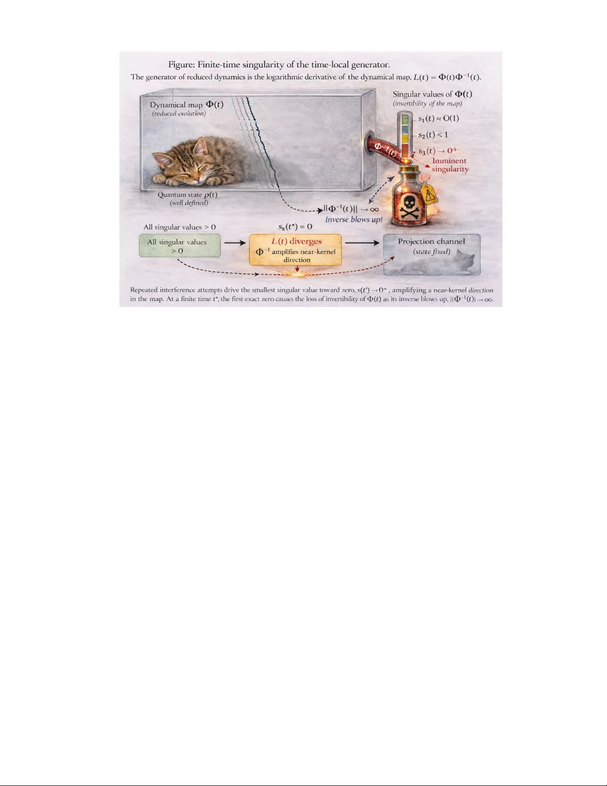
Nonp erturbativ e Resummation of Div ergen t Time-Lo cal Generators Dragomir Da vidovic 1 , ∗ 1 Scho ol of Physics, Ge or gia Institute of T e chnolo gy, USA (Dated:) Time-lo cal generators of op en quantum systems are generically divergen t at long times, even though the reduced dynamics remains regular. W e construct, by analytic con tinuation, nonpertur- bativ e dynamical maps consisten t with these generators. F or the weak-coupling un biased spin– b oson mo del, this construction yields an explicit dynamical map that nonp erturbatively resums the TCL generator and exp oses ho w the divergences signal the approac h to a singular time at whic h the reduced dynamics b ecomes nonin vertible. The reconstructed map is v alidated against TEMPO sim ulations at short times and the exactly solv able rotating-w a ve model at all times. In the full spin–b oson mo del, the same con tinuum mechanism pro duces b oth an early-time anisotrop y , with a measurable phase shift that pro vides a signature of the environmen tal correlation and the pointer direction, and a late-time singularity at which the reduced dynamics b ecomes noninv ertible. By con trast, in the rotating-wa ve mo del the map approac hes this p oin t without reaching it and remains in vertible at all times. These results establish a nonp erturbative framework for reconstructing reduced dynamics from divergen t time-lo cal generators, diagnosing the onset of noninv ertibilit y , and iden tifying experimentally accessible early-time signatures of environmen t-induced anisotrop y . I. INTR ODUCTION Reduced op en quantum system evolution is describ ed b y a completely p ositive trace -preserving (CPTP) dy- namical map Φ( t ) acting on the densit y matrix [1]. A time-lo cal master equation represen ts the same ev olution through a generator L ( t ) deﬁned b y L ( t ) = ˙ Φ( t )Φ − 1 ( t ) . (1) Th us the time-lo cal generator is the logarithmic deriv a- tiv e of the dynamical map and exists only while the map remains inv ertible. F ormally , time -local master equations are derived from the time-con volutionless pro jection-op erator expan- sion [2]. This provides one of t wo exact pro jection- op erator represen tations of reduced dynamics, the other b eing the Nak a jima–Zwanzig memory-kernel equa- tion [1]. In a cumulan t expansion for sto chastic linear diﬀer- en tial equations, the time-local generator is obtained through the cum ulant (v an Kamp en) resummation de- riv ed from the F eynman disentanglemen t theorem [3, 4]. In this method, Φ( t ) is reorganized in to an exp onen tial of cum ulants K n ( t ) that enco de progressively higher-order system–bath interactions. A remark able feature of this construction is that it remains v alid in the gen uinely quan tum regime, where interaction op erators at diﬀer- en t times do not commute. When bath correlations de- ca y suﬃcien tly rapidly , the expansion remov es the secular gro wth presen t in the Dyson series order b y order. Ho wev er, when en vironmental correlations decay slo wly , the cum ulant expansion generically diverges at long time scales, with div ergences app earing already at ∗ dragomir.davido vic@ph ysics.gatech.edu fourth order [5] and not remov ed by resummation of the leading cumulan ts [6]. This o ccurs even though the un- derlying propagator remains w ell deﬁned, consisten t with con vergence of the Dyson expansion [7]. Rather than signaling a breakdo wn of the reduced dy- namics, the divergence reﬂects the approac h to a rank c hange of the dynamical map. A singular v alue v anishes and the corresp onding time-lo cal generator b ecomes un- b ounded [Eq. (1)]. It therefore signals the approach to a noninv ertible quan tum channel, as illustrated by the Sc hr¨ odinger-cat example in Fig. 1. Once the singular time is crossed, the reduced dynamics no longer retains enough information to resurrect the initial superp osition. T o sho w that nonin v ertibility indeed o ccurs, w e exploit the fact that the resummed cumulan t expansion remains w ell deﬁned at early time scales. Its controlled gro wth at early times carries signatures of b oth an imp ending singularit y and an exp erimentally accessible anisotropy in the coherence dynamics. W e use this early-time b e- ha vior to deﬁne an analytic contin uation of the reduced dynamics. The map is then reconstructed using the F eyn- man disentanglemen t theorem, with the Da vies reference semigroup serving as the anc hor of the con tinuation. The generator is then recov ered, with its singular structure made explicit through the logarithmic deriv ative of the reconstructed map, Eq. (1). The main conceptual result of this paper then follows: in contin uum environmen ts with slowly decaying corre- lations, the same con tinuum mec hanism pro duces tw o distinct eﬀects. At early times it generates an anisotropy in the nonsecular coherence transfer, with a measurable phase shift that carries information ab out the en viron- men tal correlation and the p ointer direction. A t late times, the dynamical map reaches rank deﬁciency at ﬁ- nite time. The present metho d reveals the microscopic origin of b oth eﬀects. It lies in the coupling betw een non- secular coherence dynamics and the p ole–branch struc- ture of the bath correlation function [8]. After the Marko- 2 || FIG. 1. Finite-time loss of inv ertibility of the dynamical map induced by system–environmen t interactions. Mark ovian relax- ation, nonsecular coherence mixing, and the Khalﬁn tail jointly drive the smallest singular v alue tow ard zero. The rep eated crac k-like features reﬂect successive destructive interference b etw een the exp onen tial contribution and the bath correlation function, progressively suppressing coherence. A t the ﬁnal crack, a singular v alue v anishes, marking noninv ertibilit y . Bey ond this point, resurrection of the initial sup erp osition from the reduced dynamics is no longer possible. vian decay has b een completed and the dynamics crosses o ver to the nonexp onential deca y law [9], the secular and nonsecular coherence con tributions acquire a common asymptotic tail but cross ov er to that tail at paramet- rically diﬀerent times. The same con tinuum structure that pro duces an early observ able anisotrop y ultimately driv es the loss of inv ertibility . As a concrete illustration, w e apply the metho d to the w eak-coupling unbiased spin–boson mo del and sho w how the reconstructed dynamics exhibits b oth an early-time anisotrop y in the coherence transfer and a ﬁnite-time loss of inv ertibilit y . A useful b enchmark is provided by the exactly solv able rotating-wa v e appro ximation (R W A) mo del. In this c ase, the reduced dynamical map comes v ery close to the same singular p oint but do es not reach it b ecause of the residual phase mismatch. The R W A dynamics therefore remains in v ertible, even though it ex- hibits the same late-time nonexp onen tial deca y la w. Bey ond its role in revealing the singular structure of the generator, the present metho d oﬀers a practical computational adv antage. The disentanglemen t pro ce- dure eﬀectively separates the environmen tal modes, so their resummed inﬂuence enters p olynomially through bath correlation functions rather than via multiplicativ e Hilb ert-space embeddings. As discussed in Sec. I I I, the exp onen tial complexit y associated with Hilbert-space en- largemen t—or with inﬂuence-functional approac hes—is replaced b y polynomial scaling, establishing a fundamen- tally diﬀeren t computational strategy for op en-system dynamics. A further p oin t concerns the regime of applicabilit y of the metho d. The present approach relies on in vertible maps to diagnose the onset of noninv ertibility . This is justiﬁed by the density of inv ertible CPTP maps in the set of all CPTP maps. Any nonin vertible c hannel can b e obtained as a limit of inv ertible channels with arbitrar- ily small but nonzero coherences or p opulations in the discarded subspace. In actual calculations, the reconstructed map is ob- tained from a truncated or partially resummed cum ulant expansion. Such approximations can exhibit spurious b eha vior near the singular p oin t: the smallest singular v alue ma y reach zero and subsequently increase, artiﬁ- cially restoring inv ertibilit y . Physically , the v anishing of a singular v alue marks los s of inv ertibilit y and the as- so ciated collapse of distinguishability along a direction in state space. Any apparent restoration of inv ertibil- it y would therefore require passage through a non-CPTP regime, as shown in Sec. VI I I A. W e therefore identify the onset of noninv ertibilit y with the ﬁrst zero of the small- est singular v alue and restrict the reconstructed map to times up to this p oin t. W e now position the present approac h relative to pre- vious treatments of time-lo cal generators. In regimes where the dynamical map remains in v ertible and the gen- erator stays regular, a n umber of complementary con- 3 structions are av ailable. Explicit dilations exist for cer- tain time-lo cal quantum Marko v pro cesses [10], op erator- algebra metho ds can derive generators directly from mi- croscopic dynamics in sp eciﬁc settings [11], and related w ork seeks Lindblad generators consisten t with conserv a- tion la ws and thermalization for systems weakly coupled to baths [12]. Related exact examples also o ccur in solv- able mo dels, including linearly coupled harmonic systems in teracting with a harmonic bath [13], where the Gaus- sian structure allows the dynamical map to b e written explicitly , as well as excitation-conserving Hamiltonians suc h as the R W A, where the reduced dynamics can b e solv ed analytically [14]. A diﬀerent situation arises for contin uum environ- men ts with slowly decaying bath correlations, where late- time divergences of time-lo cal generators were ﬁrst ob- tained analytically in sp ecial infrared regimes within a fourth-order TCL expansion [5], and w ere later sho wn to b e generic rather than infrared-sp eciﬁc [6]. Anal- yses of higher-order TCL dynamics in speciﬁc mo dels further sho w that late-time non-Marko vianit y is regime dep enden t and ma y either increase or decrease at long times [15]. Existing strategies typically address these diﬃculties by mo difying the generator itself, for example through pseudoinv erse constructions [16], eﬀective-ﬁeld- theory resummations [17], or b y enforcing complete p os- itivit y via pro jection onto the nearest CPTP map [18]. The presen t work takes a complementary viewp oin t. Starting from a generator that b ecomes singular at long times, we do not attempt to regularize the singularity . Instead, w e analytically contin ue the dynamical map ob- tained from the generator and interpret the singular b e- ha vior. Outline. The remainder of the paper develops the dynamical-map reconstruction and its physical inter- pretation. W e ﬁrst formulate the reduced-dynamics framew ork and introduce the disen tangled represen tation based on a time-local generator. W e then analyze the re- constructed singularities in a rotating-wa v e b enc hmark, and ﬁnally apply the metho d to the full spin–b oson dy- namics. I I. THE ST ANDARD OPEN SYSTEM SETUP W e consider a ﬁnite–level quantum system weakly cou- pled to a bosonic environmen t. The total Hamiltonian is H T = H S + H B + H I . (2) The system Hamiltonian is diagonal in its energy eigen- basis, H S = N X n =1 E n | n ⟩⟨ n | , (3) with Bohr frequencies ω nm = E n − E m . The en vironment consists of baths of harmonic mo des H B = X k,α ω k,α b † k,α b k,α , (4) where α and k denote the bath and mo de indices, respec- tiv ely . Diﬀerent baths are assumed to b e uncorrelated. and the coupling is taken in separable form H I = X α A α ⊗ F α , (5) where A α is a dimensionless Hermitian system op erator that couples the system to bath α , normalized to hav e op erator norm of order unit y and F α = X k g k,α ( b k,α + b † k,α ) (6) is a Hermitian bath op erator with coupling constants g k,α ∝ λ ≪ 1. Bath correlations The reduced dynamics are gov erned by the bath cor- relation function C α ( t ) = ⟨ F α ( t ) F α (0) ⟩ β , (7) deﬁned with resp ect to a thermal equilibrium state at in verse temperature β . The bath is characterized b y the sp ectral density ˜ J α ω = π X k g 2 k,α δ ( ω − ω k,α ) , ω > 0 , (8) where the tilde denotes zero temp erature. W e employ the canonical contin uum environmen ts used in the spin– b oson mo del [19], ˜ J α ω = 2 π λ 2 ω s ω s − 1 c e − ω /ω c Θ( ω ) , (9) where ω c is the ultraviolet cutoﬀ frequency and s is the sp ectral exp onen t (Ohmic s = 1, sub–Ohmic 0 < s < 1, sup er–Ohmic s > 1). The thermal sp ectral density is J α ω = ˜ J α ω 1 − e − β ω , ω > 0 , (10) with the extension to negativ e frequencies ﬁxed b y de- tailed balance, J α − ω = e − β ω J α ω . (11) The bath correlation function admits the F ourier rep- resen tation C α ( t ) = 1 π Z ∞ −∞ dω J α ω e − iω t , (12) whic h at zero temp erature reduces to ˜ C α ( t ) = 2 λ 2 ω 2 c Γ( s + 1) (1 + iω c t ) s +1 . (13) 4 Half–sided transform A central quantit y is the half–sided F ourier transform Γ α ω = Z ∞ 0 dt C α ( t ) e iω t = J α ω + iS α ω , (14) whic h is analytic for Im ω > 0. Its ﬁnite-time coun terpart deﬁnes the memory kernel Γ α ω ( t ) = Z t 0 dτ C α ( τ ) e iω τ , (15) whic h is entire in ω and conv erges to Γ α ω as t → ∞ . Assumptions The analysis assumes a controlled weak–coupling op en–system limit with well separated dynamical scales. 1. We ak c oupling. λ 2 ≪ 1 , whic h is necessary for the Davies generator L 0 to pro vide the leading reduced dynamics. 2. R esolve d system fr e quencies. The bath-induced relaxation rate remains small compared with the Bohr frequencies, γ ∼ J ( ω nm ) ≪ | ω nm | . whic h in the spin–b oson mo del reduces to γ ≪ ∆. These scale separations are the necessary and suf- ﬁcien t conditions underlying the v an Ho v e weak- coupling limit and ensure the existence of a well- deﬁned p ole contribution to the dynamics. 3. Continuum envir onment. The bath is taken in the thermo dynamic limit with a contin uous sp ectral densit y (9) and ﬁnite cutoﬀ ω c , producing long– time branc h–cut contributions resp onsible for non- exp onen tial (Khalﬁn) decay . 4. Sep ar ate d timesc ales. There exists an intermediate time window T 1 , T 2 ≪ t ≪ t rec , with relaxation times T 1 , 2 and recurrence time t rec . The reconstruction and in terpretation of generator singularities apply in this regime. These conditions deﬁne the parameter domain in whic h div ergences of the time–lo cal generator are interpreted. I II. TIME-LOCAL GENERA TOR T o uncov er the structure of the divergen t generator, w e ﬁrst examine the cumulan t (v an Kampen) expansion. In this formulation the propagator can b e written as a time–ordered exp onential, Φ( t ) = T exp  Z t 0 dτ L ( τ )  , L ( t ) = ∞ X n =0 L n ( t ) , (16) where the cumulan ts L n ( t ) enco de progressively higher- order system–bath interactions [3, 4]. Eac h cum ulant eﬀectiv ely resums an inﬁnite subset of Dyson terms, so that resumming the cum ulant hierarch y amoun ts to a nested resummation of the Dyson expansion. The b eha vior of this expansion in slowly decaying en- vironmen ts was analyzed in Ref. [6]. That work show ed that resummation of the leading cumulan ts generates conjugate pairs of mo des, one exp onen tially deca ying and the other exp onentially growing. This pairing fol- lo ws from the an tisymmetry of the renormalized transi- tion frequencies inherited from the Bohr sp ectrum. As a result, the bath-induced imaginary parts enter with op- p osite signs for the tw o paired transitions: if one mo de acquires a p ositive decay rate, its conjugate necessarily acquires the opp osite rate. When environmen tal mem- ory cannot suppress the growing comp onen t, the cumu- lan t expansion diverges and the corresp onding time-local generator b ecomes unbounded. Building on Ref. [6], we construct a partially resummed TCL generator and extend the result to the case of mul- tiple uncorrelated baths, L ( t ) = − i [ H S , · ] + K ( t ) , (17) with the resummed dissipator K nm,ij ( t ) = X α A α ni A α j m  Γ α ω ( j ) in ( t ) ( t ) +  Γ α ω ( i ) j m ( t ) ( t )  ⋆  − X α,k h δ j m A α nk A α ki Γ α ω ( j ) ik ( t ) ( t ) + δ ni A α j k A α km  Γ α ω ( i ) j k ( t ) ( t )  ⋆ i , (18) where the renormalized complex frequencies are ω ( j ) in ( t ) = ω in − i h X c,α  | A α ic | 2 Γ α ω ic ( t ) − | A α nc | 2 Γ α ω nc ( t )  + X α 2 J α 0 ( t ) A α j j  A α nn − A α ii  i . (19) The ﬁrst term is the F ermi–Golden–Rule contribution, while the second term Ω α j ni ( t ) = 2 J α 0 ( t ) A α j j  A α nn − A α ii  is the sp ectral–o v erlap correction due to bath α , that cou- ples p opulations and coherences b eyond Born–Mark o v theory . F or reference, and to clarify these expressions, the explicit matrix elemen ts for the spin–boson mo del coupled to a single bath are given in App endix A. 5 The time-lo cal generator, Eq. (18), has a Redﬁeld- t yp e sup erop erator form. This do es not imply a second- order p erturbativ e approximation. F or a bilinear system– en vironment in teraction H I = A ⊗ B , eliminating the en vironmental degrees of freedom pro duces sup eropera- tors comp osed of com binations of Aρ and ρA (as well as related op erators) at all p erturbative orders. The ap- p earance of a Redﬁeld-like tensor therefore follows from the structure of the interaction Hamiltonian and from the selection of the leading cumulan ts, rather than from a truncation at O ( λ 2 ). The same op erator structure also arises in exact Gaussian TCL resummations [13]. Diﬀeren t en vironments enter the generator through the sum ov er bath indices. In structured sp ectral densities, where the index α lab els distinct environmen tal mo des coupled to the system, Mark o vian em bedding approac hes require introducing additional degrees of freedom for eac h mo de [20]. The resulting enlarged Hilbert space therefore gro ws exp onen tially with the num b er of oscillators. By con trast, the resummed TCL generator incorpo- rates the inﬂuence of each mo de through bath correla- tion functions and scales only linearly with the n um- b er of modes. The TCL approach therefore remains tractable even for highly structured environmen ts con- taining a large num b er of sp ectral features. As discussed ab ov e, this an tisymmetry pro duces paired frequency comp onents in the generator. The imaginary parts generated by the bath correlation function there- fore enter with opp osite signs for the tw o transitions. If the component associated with ω ( j ) in acquires a deca y rate γ ( j ) in ( t ) > 0, the conjugate comp onent necessarily acquires the rate − γ ( j ) in ( t ). This also implies a proliferation of renormalized frequencies through the additional index j , although this additional structure is absent in the exam- ples considered in the present pap er. Gener ator validity r ange. The generator L ( t ) ob- tained from Ref. [6] establishes an internally consistent description up to a ﬁnite time scale t L t L ≈ s + 1 ν 2 , ν 2 = 1 T 2 , where T 2 is the decoherence time. The estimate was ob- tained using a time-indep endent reference generator L M in tro duced in Ref. [6]. This time corresp onds to the min- im um of the generator deviation ∥ L ( t ) − L M ∥ : b efore t L the norm decreases, while for t > t L it b egins to increase as the gro wing modes of the generator become dominant. The Da vies generator L 0 (deﬁned b elo w) can also b e used instead of L M . The diﬀerence ∥ L M − L 0 ∥ is time- indep enden t and of order O ( λ 2 ), so b y the triangle in- equalit y the lo cation of the minimum of ∥ L ( t ) − L 0 ∥ o c- curs at the same time scale. The deﬁnition of t L is there- fore not reference-dep enden t. Thus, thereafter we use L 0 as the standard reference generator. F or t ≪ t L the time-lo cal generator approaches the Da vies w eak-coupling generator L 0 deﬁned below. As the diﬀerence L ( t ) − L 0 decreases the dynamics b ecomes eﬀectiv ely Marko vian on the v an Hov e time scale. The semigroup therefore acts as a transient ﬁxed point of the time-lo cal evolution. F or t ≳ t L the b ehavior reverses. The paired growth mo des identiﬁed ab o ve prev ail and the norm ∥ L ( t ) − L 0 ∥ b egins to increase. The generator ceases to b e a p ertur- bation of L 0 and mo ves aw a y from the Mark ovian regime. In the presen t work we eﬀectiv ely use L ( t ) as input data on the interv al t ≲ t L , where the cumulan t resummation remains con trolled but the growth mo des are already vis- ible. The dynamical map is then obtained by analytic con tinuation. The reference generator L 0 is taken to b e the Davies w eak-coupling generator [21], i.e. the Mark ovian semi- group selected by the v an Hov e weak-coupling limit of the microscopic Hamiltonian: L 0 = − i [ H S + H LS , · ] + K 0 , (20) where K 0 is the dissipator with matrix elements (see, e.g., Ref. [21, 22]) [ K 0 ] nm,ij = X α 2 A α ni A α j m δ ω in ,ω j m J α ω in − δ ni δ j m X α,k  | A α nk | 2 J α ω nk + | A α j k | 2 J α ω j k  . (21) The Lamb-shift Hamiltonian H LS has matrix elements [ H LS ] nm = δ nm X α,k | A nk | 2 S α ω nk . (22) The specialization of L 0 to the spin–boson model is giv en in Sec. VI I A. In the v an Hov e scaling τ = tλ 2 the reduced dynamics con verges to this semigroup, lim λ → 0   ρ ex ( τ /λ 2 ) − e L 0 τ /λ 2 ρ (0)   = 0 , (23) so e L 0 t pro vides provides the leading reduced dynamics in this weak-coupling sense. IV. FEYNMAN DISENT ANGLEMENT THEOREM T o determine a dynamical map whose logarithmic deriv ative repro duces the resummed time-lo cal genera- tor, we parameterize the exact map relative to the con- tractiv e reference semigroup: ρ ex ( t ) = Φ ex ( t ) ρ (0) =  e L 0 t + C ex ( t )  ρ (0) . (24) Here C ex ( t ) is an O ( λ 2 ) correction sup erop erator de- scribing deviations from the reference evolution, with C ex (0) = 0 so that Φ(0) = I .[23] The exact map satisﬁes the master equation ˙ Φ ex ( t ) = L ex ( t )Φ ex ( t ) , Φ ex (0) = 1 . (25) 6 Split the generator as L ex ( t ) = L 0 + δ L ( t ) . (26) The F eynman disentangling theorem then gives Φ ex ( t ) = e L 0 t T exp  Z t 0 dτ e − L 0 τ δ L ( τ ) e L 0 τ  . (27) Equiv alently , Φ ex ( t ) = e L 0 t T exp  Z t 0 dτ e − L 0 τ  L ex ( τ ) − L 0  e L 0 τ  . (28) Since δ L ( t ) = O ( λ 2 ), expansion to O ( λ 2 ) gives Φ ex ( t ) = e L 0 t  1 + Z t 0 dτ e − L 0 τ δ L ( τ ) e L 0 τ  + O ( λ 4 ) . (29) Inserting the factor e L 0 t in to the in tegral and compar- ing with Eq. (24), we iden tify the correction C ex ( t ) to accuracy O ( λ 2 ) as C ex ( t ) = Z t 0 dτ e L 0 ( t − τ )  L ex ( τ ) − L 0  e L 0 τ + O ( λ 4 ) . (30) The singularity of the map can mak e the n orm ∥ L ex ( t ) ∥ v ery large, but do es not pro duce a corresp onding growth of the dynamical map. Consequently the correction C ex ( t ) also remains ﬁnite. The time integral in Eq. (30) suppresses the divergence of L ex ( t ) b ecause the growth directions of the generator are w eighted by the contrac- tiv e Davies semigroup. It would therefore be incorrect to in terpret the in tegral as a regularization of the genera- tor. Rather, the forward semigroup action comp ensates the singular gro wth and reconstructs the second-order con tribution to the dynamical map. W e now make the crucial step: the same contractiv e mec hanism applies when L ex ( t ) is replaced by the par- tially resummed generator L ( t ). What app ears as an ex- p onen tially growing correction in the generator pro duces only a small con tribution to the resulting map. This mo- tiv ates deﬁning an approximate map through C ( t ) = Z t 0 dτ e L 0 ( t − τ )  L ( τ ) − L 0  e L 0 τ . (31) The net map is then written as e L 0 t + C ( t ), where the in tegral disentangles the map from the singular growth of the appro ximate generator. T o av oid repeated ter- minology , w e refer to this map interc hangeably as the r e c onstructe d or disentangle d map. In Eq. (31), the exp onentially large deviations of the generator from L 0 are increasingly suppressed b y the semigroup contraction as time progresses b ey ond t L . By con trast, for times of order t ≲ t L , where ∥ L ( t ) − L 0 ∥ is still decreasing, the growing mo des app ear only as weak eﬀects and are only partially suppressed by the contrac- tiv e dynamics. As a result, the disen tangled map eﬀec- tiv ely provides an analytic con tin uation of the resummed TCL generator, anchored in the growing mo des visible in the time window where the cum ulant construction re- mains controlled. The corresp onding reconstructed gen- erator is then obtained by taking the logarithmic deriv a- tiv e. Note that the result in Eq. (31) is nonp erturbativ e b e- cause the truncation applies only to the disentanglemen t step, not to the generator L ( t ), whic h is partially re- summed and contains nested contributions from all or- ders of the in teraction. Numerical results in this pap er w ere obtained by solving the reconstruction equation ˙ C ( t ) − L 0 C ( t ) =  L ( t ) − L 0  e L 0 t , (32) whic h is equiv alen t to Eq. (31) but pro vides improv ed n u- merical stability . The diﬀerential formulation also makes clear that the gro wing mo des of L ( t ) are preceded by the reference contraction. Also note that separating the integrand in to L ( τ ) and − L 0 parts gives C ( t ) = Z t 0 dτ e L 0 ( t − τ ) L ( τ ) e L 0 τ − Z t 0 dτ e L 0 ( t − τ ) L 0 e L 0 τ , (33) since L 0 comm utes with its exp onen tial, Z t 0 dτ e L 0 ( t − τ ) L 0 e L 0 τ = t e L 0 t L 0 . (34) Hence Φ( t ) = e L 0 t − t e L 0 t L 0 + Z t 0 dτ e L 0 ( t − τ ) L ( τ ) e L 0 τ = e L 0 t  I − tL 0 + Z t 0 dτ e − L 0 τ L ( τ ) e L 0 τ  . (35) The last pair of equations sho w that the disentangle- men t pro cedure necessarily pro duces a linear-in-time con- tribution prop ortional to tL 0 . A purely exp onential de- ca y therefore requires that the contribution generated b y L ( τ ) provide an equal and opp osite linear term. The exis- tence of exp onen tial relaxation thus imposes a constraint on the generator, as will b e seen in the applications b e- lo w. V. R W A MODEL AND EXACT DYNAMICS W e consider the spin-b oson mo del H = H S + H B + H I , H S = ∆ 2 σ z , H I = A ⊗ F . (36) W e sp ecialize to unbiased transv erse coupling, A = 1 2 σ x . (37) Throughout the main text w e further restrict to zero temp erature. Excitation pro cesses are then absent, so 7 an y loss of inv ertibilit y of the reduced dynamics cannot b e attributed to thermal mixing and must instead orig- inate from coherent system–bath interaction. In several expressions we write the matrix element A 2 12 explicitly as 1 / 4; this factor should b e understoo d as A 2 12 , A 2 21 , or | A 12 | 2 , dep ending on con text, and th us the formal- ism extends trivially to an arbitrary transverse coupling direction. In the rotating-wa v e approximation we retain only n umber-conserving terms, H I ≈ 1 2 ( σ + ⊗ F − + σ − ⊗ F + ) , (38) F + = X k g k b † k , F − = X k g ∗ k b k , (39) so that the total excitation n um b er N = σ + σ − + P k b † k b k is conserved. At T = 0 the dynamics from a single- excitation preparation is therefore conﬁned to the N = 1 sector. F or an initial sup erp osition | Ψ(0) ⟩ = c 1 | 1 ⟩ + c 2 | 2 ⟩ , | c 1 | 2 + | c 2 | 2 = 1 , (40) the exact reduced state has the form [14] ρ exact ( t ) =  | c 1 f ( t ) | 2 c 1 c ∗ 2 f ( t ) c ∗ 1 c 2 f ∗ ( t ) 1 − | c 1 f ( t ) | 2  , (41) corresp onding to the quantum dynamical map Φ f ( t ) =    | f ( t ) | 2 0 0 0 1 − | f ( t ) | 2 1 0 0 0 0 f ⋆ ( t ) 0 0 0 0 f ( t )    , (42) in the ordering ( ρ 11 , ρ 22 , ρ 21 , ρ 12 ). So all reduced dynam- ics is determined by the surviv al amplitude f ( t ). The coherence sector contributes t wo singular v alues equal to | f | , while the p opulation blo ck yields one singular v alue of order | f | 2 , and one of order unity . Hence, as f ( t ) → 0 three singular v alues sim ultaneously v anish and the map approac hes a rank-one pro jection. The time–lo cal generator is obtained by inserting Eq. (42) into Eq. (1): L f ( t ) =       ˙ f f + ˙ f ⋆ f ⋆ 0 0 0 − ˙ f f − ˙ f ⋆ f ⋆ 0 0 0 0 0 ˙ f ⋆ f ⋆ 0 0 0 0 ˙ f f       . (43) Consequen tly the time-lo cal generator div erges at the ze- ros of the surviv al amplitude. In the R W A mo del, the transverse Blo ch comp onent satisﬁes x ( t ) − iy ( t ) = 2 ρ 12 ( t ) = f ( t ) [ x (0) − iy (0)] . Th us the evolution acts on the ( x, y ) plane as an isotropic con traction com bined with a rotation. In the in teraction picture, f I ( t ) = e − i ∆ t f ( t ) obeys the exact V olterra equation ˙ f I ( t ) = − 1 4 Z t 0 dτ C ( t − τ ) e i ∆( t − τ ) f I ( τ ) . (44) Equation (44) is iden tical to the surviv al–amplitude equation derived by Peres for quantum decay in to a con- tin uum sp ectrum [9]. In such systems the surviv al ampli- tude contains tw o distinct comp onents: an exp onen tial term asso ciated with a p ole of the resolven t, and a de- la yed correlation term arising from the contin uum sp ec- trum. As ﬁrst shown b y Khalﬁn [8], the con tinuum part necessarily pro duces non-exp onen tial long-time behavior. In the presen t mo del the same p ole and branch–cut struc- ture appears through the bath correlation function C ( t ), whic h generates an algebraic tail that interferes with the exp onen tial p ole contribution. The explicit solution in the Sc hr¨ odinger picture is [14] f ( t ) = 1 4 π Z ∞ 0 dω e − iω t J ω (∆ − ω + S ω / 4) 2 + ( J ω / 4) 2 . (45) The integral representation conﬁrms that the coherence amplitude remains ﬁnite and smo oth for all times. Thus, a divergence of the logarithmic deriv ativ e ˙ f ( t ) /f ( t ) can o ccur only when the denominator b ecomes arbitrarily small. This realizes the mechanism an ticipated in the In tro duction: the reduced state remains regular while the dynamical map approaches loss of inv ertibilit y , and the singularity app ears only in the logarithmic generator represen tation. Equation (45) makes explicit that the surviv al ampli- tude is a F ourier transform of a b ounded sp ectral densit y determined by the bath. Consequently the late-time b e- ha vior cannot remain purely exp onen tial and must cross o ver to the algebraic decay . FIG. 2. Represen tative long-time dynamics of the coherence amplitude | f ( t ) | . (a,b) Log–linear and log–log plots show- ing the crossov er from exp onen tial (Marko vian) to p ow er-law (non-Mark ovian) decay . Near the phase lo c k-in time t P , in- terference pro duces oscillations. Black: Ohmic bath ( s = 1, λ 2 = 0 . 025); red: sub-Ohmic bath ( s = 1 / 3, λ 2 = 0 . 01). In b oth cases ω c = 4, ∆ = 1. Represen tative exact solutions for several sp ectral ex- p onen ts are shown in Fig. 2. The coherence magni- tude | f ( t ) | crosses from an initial exp onential decay to 8 a late-time algebraic tail at the time scale t P , deﬁned b y Eq. (50). Near t P , destructive in terference b et ween these t wo con tributions pro duces deep minima in | f ( t ) | . A. P ole–plus–tail interference In the weak–coupling regime the integrand in Eq. (45) is is sharply p eaked near ˜ ∆ = ∆ + S (∆) / 4. Expanding ab out this p eak yields a Loren tzian lineshap e and the Wigner–W eisskopf (Mark ovian) exp onential contribution f M ( t ) = e − [ i ˜ ∆+ J ∆ / 4] t , (46) whic h accurately describ es the coherence for t ≲ t P . A t late times the dominan t frequencies scale as ω ∼ 1 /t , and the lineshap e in Eq. (45) is con trolled b y its lo w–frequency b ehavior. Rapidly oscillating contribu- tions av erage out and only the low-frequency part of the sp ectrum survives. Appro ximating the denominator by its ω = 0 v alue then giv es the tail f C ( t ) ≈ 1 4[∆ + S 0 / 4] 2 , C ( t ) , (47) whic h captures the algebraic decay for t ≳ t P . The ex- act coherence is therefore w ell approximated by the t wo– comp onen t form f ( t ) ≈ f M ( t ) + f C ( t ) . (48) Destructiv e interference b et ween f M and f C pro duces times at which f ( t ) b ecomes anomalously small, ap- proac hing the kernel of the dynamical map. The time t P follo ws from the balance betw een the Mark ovian p ole contribution and the long–time tail, | f M ( t P ) | = | f C ( t P ) | . F rom Eq. (46) one has | f M ( t ) | = e − t/T 2 , while the bath correlator for a sp ectral density J ( ω ) ∝ ω s e − ω /ω c yields the asymptotic tail | f C ( t ) | ∝ ( ω c t ) − ( s +1) . Equating the t wo giv es e − t P /T 2 ∼ ( ω c t P ) − ( s +1) , (49) so that t P T 2 ∼ ( s + 1) ln( ω c t P ) . In the weak–coupling regime ω c T 2 ≫ 1, replacing t P in- side the logarithm by T 2 up to subleading lnln corrections yields t P ∼ ( s + 1) T 2 ln( ω c T 2 ) ∼ ( s + 1) T 2 ln 1 λ 2 . (50) Near t P , interference b et w een f M and f C pro duces nar- ro w modulation windo ws in | f ( t ) | , ranging from transient bursts to near–extinctions and accompanied by near- π phase slips at destructive interference [Fig. 3(a,b)]. FIG. 3. Coherence magnitude (a) and phase (b) near t P in the R W A mo del. Constructive interference pro duces bursts, while destructive interference leads to near-extinction. The phase undergo es a rapid rotation approaching a π slip, con- sisten t with the map remaining inv ertible. Red dotted: ex- act solution; blac k solid: tw o-component mo del. Parameters: s = 1 / 3, λ 2 = 0 . 01, ω c = 4, ∆ = 1. The dynamical map b ecomes strictly non-in vertible only if f ( t ) = 0 at a ﬁnite time. F or a con tinuum environ- men t this requires exact destructive in terference b et ween the p ole con tribution and the bath-correlation tail. Such cancellation requires ﬁne tuning of sp ectral phases and is therefore non-generic for con tinuum R W A-Hamiltonians. The interference pro duces v ery small but nonzero v al- ues of f ( t ), so the map remains inv ertible at all ﬁnite times while approaching a non-in v ertible channel asymp- totically . VI. R W A CUMULANT EXP ANSION A. Reference and TCL Generators W e now apply the general cum ulant analysis to the R W A V olterra equation (44) using the v an Kamp en ordered-cum ulant expansion. As in the general case, for algebraically deca ying bath correlation functions, cumu- lan ts beyond a critical order n max ( s ) display late-time gro wth [6]. Resumming the leading growing cumulan ts reorganizes this algebraic gro wth in to an exp onential time dep endence. This leading resummation is a spe- cial case of the complex renormalization introduced in Eq. (19) and deﬁnes the inﬂated TCL generator. Details are presented in App endix B. The time-dep endent renormalized frequency is given 9 b y u ( t ) = ω − i 4 Γ ω ( t ) , (51) while the surviv al amplitude in the in teraction picture satisﬁes ˙ f I f I      resum = − 1 4 Γ u ( t ) ( t ) + O ( λ 4 ) . (52) The Sc hr¨ odinger-picture partially resummed generator is then obtained from Eq. (43) by replacing ˙ f /f with its resummed counterpart, yielding L ( t ) =  L pop ( t ) 0 0 L coh ( t )  , (53) in the vectorization order ρ 11 , ρ 22 , ρ 21 , ρ 12 . Here L pop ( t ) = 1 2  − Re Γ u ( t ) ( t ) 0 Re Γ u ( t ) ( t ) 0  , (54) and L coh ( t ) =  i ∆ − 1 4 Γ ⋆ u ( t ) ( t ) 0 0 − i ∆ − 1 4 Γ u ( t ) ( t )  . (55) The generator exhibits exp onen tial gro wth at long times, since Im u ( t ) < 0 as t → ∞ . R emark The full ordered-cumulan t resummation con- tains nested renormalizations (App endix B) that can shift the renormalized frequency onto a diﬀeren t analytic branc h, u = ω − i 4 Γ ω − i 4 Γ ω − i 4 Γ ω − ... , (56) where w e suppress the time dep endence for clarity . Such branc h shifts can qualitatively mo dify the long-time structure of the resummation, including its inv ertibil- it y prop erties. In the present work we restrict the re- construction to the analytic branch Eq. (51) that is con tinuously connected to the weak-coupling (Da vies) limit. This choice preserves contin uity with the micro- scopic weak-coupling theory and deﬁnes the branch used throughout. The role of the self-consistent renormaliza- tions in Eq. (56) is left for future work. B. Disen tangled Map for the R W A F or the R W A Hamiltonian, the Da vies generator de- comp oses into population and coherence sectors, ( L 0 ) pop = 1 2  − J ∆ 0 J ∆ 0  , (57) and ( L 0 ) coh =  i ˜ ∆ − 1 4 J ∆ 0 0 − i ˜ ∆ − 1 4 J ∆  . (58) Because [ L ( t ) , L 0 ] = 0, the reconstruction in tegral (31) simpliﬁes to C ( t ) = e L 0 t Z t 0 dτ [ L ( τ ) − L 0 ] . (59) W e deﬁne the complex Bohr frequency z = ∆ − i 4 Γ ∆ . (60) Using the explicit matrices ab o ve, the reconstructed coherence amplitude f ( t ) = ρ 12 ( t ) /ρ 12 (0) b ecomes f ( t ) =  1 + Γ ∆ 4 t  e − iz t − 1 4 e − iz t Z t 0 dτ Γ u ( τ ) ( τ ) . (61) The linear prefactor in front of the ﬁrst exp onen tial in Eq. (61) originates from the disentanglemen t identit y Eq. (35). Its cancellation is clariﬁed b elow. 1. Markovian Appr oximation for the F r e quency T o obtain a closed analytic description of the dynam- ics, we consider the asymptotic regime t ≫ τ C , where τ C ≡ 1 /ω c is the bath correlation time. The condi- tion t ≫ τ C is typically asso ciated with the onset of the Mark ovian limit [24]. In the regime t ≫ τ C w e freeze the frequency renor- malization in Eq. (51) at its asymptotic v alue and treat the p ole as time indep enden t, u ( t ) → z . This is justiﬁed because the bath correlation function has already decay ed on the scale τ C , so the self-energy con- tribution entering u ( t ) has reached its stationary limit. In contrast, we retain the explicit time dep endence of the memory kernel in Eqs. (54) and (55). The cumulan t in tegral contin ues to grow and pro duces the large loga- rithmic deriv ativ e Γ z ( t ) even after the renormalized fre- quency has saturated. Consequently the late-time b ehav- ior is gov erned b y a stationary p ole but a time-dependent generator. The resulting surviv al amplitude simpliﬁes to f ( t ) =  1 + 1 4 Γ ∆ t  e − iz t − 1 4 Σ z ( t ) , (62) where Σ z ( t ) = Z t 0 dτ τ C ( t − τ ) e − iz τ (63) is termed the diagonal kernel. It gov erns the late-time nonexp onen tial decay of the surviv al amplitude. The diagonal kernel admits the con tour representation Σ z ( t ) = − 1 2 π Z ∞ + iγ −∞ + iγ dω e − iω t Γ ω ( z − ω ) 2 , (64) where the contour oﬀset iγ lies ab ov e all singularities of the integrand. This form pro vides the starting p oin t for the asymptotic analysis b elow. 10 2. Wigner–Weisskopf R e gime T o leading order in λ 2 , the contour in tegral in Eq. (64) yields the surviv al amplitude f ( t ) = e − iz t + 1 4 π Z ∞ 0 dω e − iω t δ J ω ( z − ω ) 2 , (65) where δ J ω = J ω − J ∆ . The p ole contribution together with the on–shell part of the branch cut on ω ∈ R + cancels the linear term Γ ∆ t/ 4 generated by the disentanglemen t theorem, leav- ing the pure exponential decay of the v an Hov e limit. The remaining integral is the residual branc h–cut correction. 3. Khalﬁn R e gime A t long times the p ole contribution has fully deca yed, and the dynamics is go v erned entirely b y the contin- uum comp onen t. The remaining amplitude is there- fore determined by the highly oscillatory F ourier integral in (65), whose leading b eha vior is controlled b y the ana- lytic structure of the sp ectral density . One obtains f ( t ) ≃ C ( t ) 4 z 2 , (66) so that the coherence amplitude is directly prop ortional to the bath correlation function. This agrees, up to O ( λ 2 ) corrections in z , with the Khalﬁn long-time tail of the exact solution (47). C. Exact Solution versus Con tinuation Figure 4 veriﬁes the analytic contin uation pro cedure b y solving the reconstruction equation (32) numerically , without inv oking the asymptotic approximation t ≫ τ C . P anel (a) sho ws the ea rly-time generator matrix ele- men t L 11 , 11 ( t ) obtained from the resummed TCL expan- sion and from the exact solution. The agreement demon- strates that the TCL generator captures the correct an- alytic structure at short times. This regime was termed “secular inﬂation” in Ref. [6], but that description is mis- leading in this time range, since the growth is ph ysical and repro duced by the exact solution. P anel (b) fo cuses on the time t P where destructive in terference strongly suppresses the surviv al amplitude f ( t ) and the dynamical map b ecomes nearly singular. The generator reconstructed from the dynamical map matc hes the exact generator b efore, at, and after the spik e, except at the very near-singular p eaks. The agree- men t b eyond the spike reﬂects that the map remains in- v ertible, allowing the contin uation pro cedure to recov er the correct generator across the near-singular region. FIG. 4. Numerical v alidation of the con tinuation pro cedure. (a) Early-time generator element L 11 , 11 ( t ): re- summed TCL (blue) agrees with the exact result (red). (b) Near t P , destructive in terference suppresses f ( t ) and pro duces a sharp generator spike. The generator reconstructed from the disen tangled map (black) repro duces the exact result (red) b e- fore, at, and after the spike. Parameters: s = 1 / 3, λ 2 = 0 . 01, ω c = 4, ∆ = 1, T = 0. D. F rom the R W A to the F ull Spin–Boson Mo del With the R W A benchmark in hand, w e now turn to the full spin–boson mo del. The R W A b enchmark isolates the mec hanism resp onsible for the generator spike: in terfer- ence b etw een the exp onen tial p ole and the algebraic cor- relation tail strongly suppresses the surviv al amplitude f ( t ) and drives the dynamical map close to singularity . The map nevertheless remains inv ertible at all times, ex- cept for a measure-zero set of phase-matching conditions, admitting analytic contin uation across the full time do- main. In the full spin–b oson mo del, how ev er, counter– rotating terms induce nonsecular coherence transfer and in tro duce an anisotropy that b ecomes pronounced in the Khalﬁn regime. The resulting interference then conv erts the near-singular b eha vior of the surviv al amplitude into a true singularity . VI I. FULL SPIN-BOSON MODEL W e now consider a tw o–lev el system coupled to a b osonic en vironmen t through the full interaction term A = σ x / 2 in the Hamiltonian Eq. (36). The coupling op erator A is the qubit observ able to which the en vi- ronmen t is sensitive. Information ab out the eigenstates 11 of A leaks into the bath, suppressing distinguishabilit y b et w een states that diﬀer primarily along this direction. The central questions are: (i) what signatures of this anisotrop y appear in the dynamics, and (ii) whether this suppression approac hes rank deﬁciency only asymptoti- cally , as in the R W A Hamiltonian, or reac hes a nonin- v ertible p oin t at ﬁnite time. A. Reference and TCL Generators in the SBM The reference generator is given by Eqs. (57) and (58), with ˜ ∆ = ∆ + 1 4 ( S ∆ − S − ∆ ) including the correct Lamb shift, in con trast to the naiv e rotating-w av e appro ximation [25]. In the reference dy- namics, the coherence evolv es as a uniform contraction at rate J ∆ / 4 combined with a rotation at frequency ˜ ∆. Because the contraction is isotropic, the singular v alues of the transverse propagator are equal and strictly p ositiv e for any ﬁnite time. Consequently the reference channel Φ 0 ( t ) remains inv ertible for all t < ∞ . The TCL generator matrix elements are obtained by sp ecializing the results of App endix A to the unbiased spin–b oson mo del at zero temp erature. The p opulation and coherence dynamics decouple, so the TCL generator reads L ( t ) =  L pop ( t ) 0 0 L coh ( t )  . (67) The generator dep ends on a time–dep endent renormal- ized transition frequency ∆ ′ ( t ) = ∆ − i 4 (Γ ∆ ( t ) − Γ − ∆ ( t )) . (68) F or times t ≫ τ C the frequency approaches its Marko- vian limit ∆ ′ ( ∞ ) ≡ a = ∆ − i 4  Γ ∆ + Γ ∗ − ∆  = ˜ ∆ − i 4 J ∆ . (69) In the following, analytical computations are p er- formed within this Mark o v approximation for the fre- quency . Numerical computations, ho wev er, are carried out without this approximation by solving Eq. (32) di- rectly . F or compactness we introduce the notation Γ ± ( t ) ≡ Γ ± ∆ ′ ( t ) ( t ) . The coherence blo ck then takes the form L coh ( t ) =  ℓ 21 , 21 ( t ) ℓ 21 , 12 ( t ) ℓ 12 , 21 ( t ) ℓ 12 , 12 ( t )  , (70) with matrix elements ℓ 12 , 12 ( t ) = − i ∆ − 1 4  Γ + ( t ) + Γ ∗ − ( t )  , (71) ℓ 21 , 12 ( t ) = 1 4  Γ + ( t ) + Γ ∗ − ( t )  , (72) ℓ 21 , 21 ( t ) = ℓ ∗ 12 , 12 ( t ) (73) ℓ 12 , 21 ( t ) = ℓ ∗ 21 , 12 ( t ) . (74) The diagonal elements contain the Bohr frequency ∆ together with the dissipative combination Γ + ( t ) + Γ ∗ − ( t ), whic h go verns the decay of the coherence amplitudes. By con trast, the oﬀ–diagonal elements ℓ 21 , 12 ( t ) and ℓ 12 , 21 ( t ) generate nonsecular transfer b etw een the tw o coherence comp onen ts ρ 12 and ρ 21 . The dissipative parts of the secular and nonsecular sectors ha ve equal magnitude and opp osite sign, whereas only the secular rates con tains the unitary splitting − i ∆. More generally , for a transverse coupling A = 1 2  σ ·  a in the plane orthogonal to the energy basis, the nonsecular coupling acquires a phase set by the p ointer direction  a . The choice A = σ x / 2 used here yields a real coupling, whereas A = σ y / 2 would yield a purely imaginary one. By contrast, the diagonal decay rates are indep endent of the p oin ter direction. The anisotropy of the coherence dynamics is therefore carried by the phase of the nonsec- ular coherence channel. The p opulation blo ck has an analogous structure, L pop ( t ) =  ℓ 11 , 11 ( t ) ℓ 11 , 22 ( t ) ℓ 22 , 11 ( t ) ℓ 22 , 22 ( t )  , (75) with matrix elements ℓ 11 , 11 ( t ) = − 1 2 Re Γ + ( t ) (76) ℓ 11 , 22 ( t ) = 1 2 Re Γ − ( t ) (77) ℓ 22 , 11 ( t ) = − ℓ 11 , 11 ( t ) (78) ℓ 22 , 22 ( t ) = − ℓ 11 , 22 ( t ) . (79) B. Disen tangled Map Substituting the generator into the disentanglemen t form ula Eq. (31) yields the matrix elements of the dy- namical map. The intermediate algebra is given in the App endix D. In the coherence sector tw o distinct comp onen ts ap- p ear, Φ 12 , 12 ( t ) =  1 + Γ ∆ + Γ − ∆ 4 t  e − i ˜ ∆ t − J ∆ 4 t − 1 4 e − i ˜ ∆ t − J ∆ 4 t Z t 0 dτ  Γ ∆ ′ ( τ ) ( τ ) + Γ ⋆ − ∆ ′ ( τ ) ( τ )  , (80) and Φ 21 , 12 ( t ) = 1 4 e i ˜ ∆ t − J ∆ 4 t Z t 0 dτ e − 2 i ˜ ∆ τ ×  Γ ∆ ′ ( τ ) ( τ ) + Γ ∗ − ∆ ′ ( τ ) ( τ )  . (81) The diagonal component contains the reference semi- group con tribution together with a memory correction, whereas the oﬀ–diagonal comp onen t is generated en tirely b y the bath memory . 12 The other matrix elements are obtained by complex conjugation, Φ 21 , 21 = Φ ∗ 12 , 12 and Φ 12 , 21 = Φ ∗ 21 , 12 . The linear prefactor in Eq. (80) is a non–Mark ovian term gen- erated by the disentanglemen t theorem [see Eq. (35)]. It will b e canceled by the integral contribution, restoring the v an Hov e limit. The p opulation dynamics can b e reconstructed using the same disentanglemen t pro cedure as in the coherence sector. The calculation is algebraically more cum bersome b ecause the p opulation blo c k couples the tw o diagonal comp onen ts of the densit y matrix, so the main results are summarized in Subsubsection VI I E, while the full deriv ation is deferred to App endix D 3. C. Diagonal Coherence Dynamics The resulting in tegrals are ev aluated in the Mark ov appro ximation for the frequency argument. The diagonal coherence element b ecomes Φ 12 , 12 ( t ) =  1 + Γ ∆ + Γ ∗ − ∆ 4 t  e − iat − 1 4 Σ sbm a ( t ) , (82) where Σ sbm a ( t ) = Σ a ( t ) + e − J ∆ t/ 2 [Σ − a ( t )] ∗ , (83) with Σ a ( t ) deﬁned in Eq. (63). The tw o terms represent the emission and absorption contributions, resp ectiv ely . As in the R W A, the diagonal k ernel admits the con tour represen tation Σ sbm a ( t ) = − 1 2 π Z ∞ + iγ −∞ + iγ dω e − iω t Γ ω +  Γ − ω ∗ + iJ ∆ / 2  ∗ ( ω − a ) 2 . (84) where the contour oﬀset iγ lies ab ov e all singularities of the integrand. 1. Diagonal Wigner–Weisskopf R e gime in the SBM As in the R W A, to leading order in λ 2 the con tour in tegral yields [Φ( t )] 12 , 12 = e − iat + 1 4 π Z ∞ 0 dω  e − iω t δ J ω ( a − ω ) 2 + e iω t − J ∆ t/ 2 J ω ( a ∗ + ω ) 2  , (85) where δ J ω = J ω − J ∆ . The p ole contribution together with the on–shell part of the branch cut on ω ∈ R + cancels the linear term (Γ ∆ + Γ ∗ − ∆ ) t/ 4 generated by the disen tanglement theorem, leaving the pure exp onen tial deca y of the v an Hov e limit. The remaining integral is the residual branch–cut correction. 2. Diagonal Khalﬁn R e gime in the SBM A t long times t → ∞ , the dominant frequencies scale as ω ∼ 1 /t , so the denominators may b e expanded in ω . The leading term is then prop ortional to the bath correlation function, and the resulting Khalﬁn tail is [Φ( t )] 12 , 12 = 1 4∆ 2 h C ( t ) + e − J ∆ t/ 2 C ( t ) ∗ i . (86) 3. Pole–plus–tail interfer enc e Com bining the exponential and algebraic contributions yields the interpolation formula Φ 12 , 12 ( t ) ≈ e − iat + 1 4∆ 2 h C ( t ) + e − J ∆ t/ 2 C ( t ) ∗ i , (87) v alid for t ≫ τ C . The absorption contribution in Eq. (87) is subleading relativ e to the reference exp onential e − iat and therefore has little eﬀect on the observ able dynamics. Keeping only the leading part of each con tribution, one may write Φ 12 , 12 ( t ) ≈ e − iat + C ( t ) 4∆ 2 , (88) whic h provides a uniformly accurate interpolation for t ≫ τ C . Up to this p oin t, the structure remains essen tially the same as in the R W A mo del. D. Oﬀ–diagonal coherence dynamics The oﬀ–diagonal element diﬀers qualitatively from the R W A case and therefore requires a separate analysis. It is central to the main results: anisotropy , the emergence of the p oin ter direction, pro jective behavior, and the loss of inv ertibilit y . Since the oﬀ–diagonal map elemen t is O ( λ 2 ), replacing ˜ ∆ b y ∆ in nonoscillatory prefactors and denominators c hanges the result only at O ( λ 4 ). W e mak e this replace- men t as con venien t in the deriv ation, while retaining ˜ ∆ in oscillatory phases and trigonometric functions, where the Lamb shift contributes to the long-time phase. In the Marko v approximation for the frequency , Eq. (81) can b e rewritten as Φ 21 , 12 ( t ) = 1 4 h Z a ( t ) + e − J ∆ t/ 2 [ Z − a ( t )] ∗ i , (89) where we introduced the oﬀdiagonal k ernel Z x + iy ( t ) = Z t 0 dτ C ( t − τ ) sin( xτ ) x e y τ . (90) T aking the Laplace transform and inv erting along the Brom wich con tour gives Φ 21 , 12 ( t ) = − 1 8 π Z ∞ + iγ −∞ + iγ dω e − iω t Γ ω +  Γ − ω ∗ + iJ ∆ / 2  ∗ ( ω + iJ ∆ / 4) 2 − ˜ ∆ 2 . (91) 13 The result separates naturally into p ole and branch–cut con tributions. 1. Oﬀ-diagonal Wigner–Weisskopf r e gime in SBM Pole c ontribution. Ev aluating the residues at ω ± = ± ˜ ∆ − iJ ∆ / 4 yields Φ pole 21 , 12 ( t ) = i 8 ˜ ∆ e − J ∆ t/ 4 h e − i ˜ ∆ t  Γ a + (Γ − a ) ∗  (92) − e + i ˜ ∆ t  Γ − a ⋆ + (Γ a ⋆ ) ∗ i . (93) In the weak–coupling limit a → ∆ − i 0 + , this reduces to Φ pole 21 , 12 ( t ) = − i 4 e − J ∆ t/ 4 cos( ˜ ∆ t ) ∆ (Γ ∗ ∆ + Γ − ∆ ) , (94) whic h traces a one–dimensional tra jectory in the complex plane. Br anch–cut c ontribution. The emission and absorp- tion contin ua give Φ cut 21 , 12 ( t ) = − 1 4 π Z ∞ 0 dω e − iω t J ω ( ω + iJ ∆ / 4) 2 − ˜ ∆ 2 − e − J ∆ t/ 2 4 π Z ∞ 0 dω e iω t J ω ( ω + iJ ∆ / 4) 2 − ˜ ∆ 2 . (95) Unlik e the diagonal sector, the resolv ent has only ﬁrst- order p oles. The on-shell and oﬀ-shell contributions can nev ertheless b e determined by contour deformation, as sho wn in Subsubsection D 2 d of App endix D. One ﬁnds the on-shell contribution Φ cut , em 21 , 12 ( t ) = iJ ∆ 4∆ e − J ∆ t/ 4 e − i ˜ ∆ t (96) v alid to O ( λ 2 ). The absorption integral has no p ole in the upp er half–plane and therefore pro duces only subleading oﬀ–resonan t con tributions. Adding Eq. (96) to the p ole term (94) yields the p ole plus on–shell contribution Φ pole+shell 21 , 12 ( t ) = e − J ∆ t/ 4 X ( t ) , (97) where X ( t ) is a real function X ( t ) = 1 4∆ h J ∆ sin( ˜ ∆ t ) − ( S ∆ − S − ∆ ) cos( ˜ ∆ t ) i = 1 4 | Γ ∆ + Γ ∗ − ∆ | ∆ sin( ˜ ∆ t − θ ) = X 0 sin( ˜ ∆ t − θ ) . (98) The phase is determined b y the ratio of the Lamb shift to the sp ectral density , θ = tan − 1 S ∆ − S − ∆ J ∆ . (99) Th us the tra jectory of Φ pole+shell 21 , 12 lies on the real axis in the complex plane. Because part of this anisotropy arises from the branch-cut contribution, the phase shift is not determined solely b y the p ole structure, but al- ready carries a signiﬁcan t imprint of the contin uum en- vironmen t. As a result, a p ole-only treatment such as Blo c h–Redﬁeld misses part of the anisotropy and pre- dicts a diﬀerent phase structure. 2. Comp arison with Blo ch–R edﬁeld dynamics Blo c h–Redﬁeld dynamics misses the branc h-cut part of the anisotropy . In this case, the transfer amplitude Φ 21 , 12 ( t ) b ecomes complex, with a phase that diﬀers from that of the disentangled map. The Blo ch–Redﬁeld map can be constructed explicitly b y applying the disen tanglement pro cedure of Sec. IV to the Bloch–Redﬁeld generator. This generator is obtained from the partially resummed TCL generator b y replacing the renormalized frequency (19) with the bare transition frequency in the dissipator (18). F or example, Eq. (81) giv es, in the Marko vian approximation, l 21 , 12 ( τ ) → Γ ∆ + Γ ∗ − ∆ 4 . The corresp onding nonsecular map element follows di- rectly from Eq. (81) by replacing Γ ∆ ′ ( τ ) ( τ ) + Γ ∗ − ∆ ′ ( τ ) ( τ ) → Γ ∆ + Γ ∗ − ∆ and p erforming the elementary in tegral: Φ BR 21 , 12 ( t ) = e − J ∆ t/ 4 X B R ( t ) , (100) with X B R ( t ) = X 0 e iθ sin( ˜ ∆ t ) . (101) The tra jectory of Φ BR 21 , 12 ( t ) therefore lies along a line ro- tated by an angle θ with resp ect to the real axis, with no phase oﬀset in the oscillation. F or consistency with n umerical calculations that do not emplo y the Mark ovian approximation for the fre- quency , we also solv e the Blo c h–Redﬁeld master equation with time-dep endent co eﬃcients in the numerical simu- lations [26]. The diﬀerence b etw een Eqs. (98) and (101) is b oth qualitativ e and signiﬁcant. In the disentangled map, the anisotrop y is enco ded as a phase shift of oscillations along the p ointer axis. In Blo c h–Redﬁeld dynamics, b y con- trast, the same anisotrop y app ears instead as a rotation of the oscillation axis, with no phase shift. Although the Blo c h–Redﬁeld generator is accurate to O ( λ 2 ), the coherence dynamics it generates need not b e accurate to that order. Related inconsistencies of Blo c h–Redﬁeld dynamics ha ve b een discussed previously for population dynamics [5, 27 – 29]. Here the same is- sue arises in the coherence dynamics, not only quanti- tativ ely but also qualitativ ely , since Blo ch–Redﬁeld can 14 ev en predict the wrong anisotropy direction. This may app ear to contradict the fact that the asymptotic co- herence in Bloch–Redﬁeld dynamics remains accurate to O ( λ 2 ) [5, 27 – 29]. How ever, the asymptotic amplitude can b e correct ev en if the tra jectory is not. More gen- erally , this sho ws that correcting a master equation to repro duce the exp ected asymptotic state do es not by it- self guarantee dynamical accuracy [30]. The diﬀerences b et ween the Blo c h–Redﬁeld, disentan- gled, and n umerically exact TEMPO (time-evolving ma- trix pro duct op erator) dynamics [31] are illustrated in Fig. 5. T o compare the oscillations, we pro ject Φ BR 21 , 12 ( t ) on to its maximal quadrature by rotating out the trivial oscillatory phase, ˜ Φ BR 21 , 12 ( t ) = e − iθ Φ BR 21 , 12 ( t ) . (102) This aligns the signal with the direction of maximal os- cillation amplitude, for which the orthogonal quadra- ture v anishes, as would be done exp erimentally when the p oin ter basis is not kno wn a priori. The TEMPO results agree very closely with the disentangled map prediction, while the Blo c h–Redﬁeld results exhibit a systematic de- viation due to the absence of the phase shift. The amplitude of this anisotrop y eﬀect in Φ 21 , 12 is O ( λ 2 ), but in this channel it con tributes at leading order, since the reference contribution v anishes. It therefore ap- p ears already at early times, b efore the ov erall signal is strongly suppressed by exp onen tial deca y , and is in prin- ciple accessible by quan tum pro cess tomograph y . Measuring the asso ciated phase provides direct access to the bath correlation function and an early signature of the pointer direction. F or example, in the scaling limit ω c → ∞ for an Ohmic bath, θ → − π / 2. In this regime, a detector coupled to a broadband electromagnetic en- vironmen t, suc h as an Unruh–DeWitt detector, should exhibit the corresponding phase shift in its coherence dy- namics. 3. Oﬀ-Diagonal Khalﬁn T ail in the SBM The remaining oﬀ–shell con tinuum con tribution to the disen tangled map is ev aluated in Subsection D 2 of Ap- p endix D. Adding this contribution to the exp onen tial part in Eq. (97) gives Φ 21 , 12 ( t ) = e − J ∆ t/ 4 X ( t ) + C ( t ) 4∆ 2 . (103) This expression shares the same asymptotic tail as the diagonal coherence element in Eq. (88). This reveals a sharp contrast b et ween the Marko vian regime and the late-time Khalﬁn-tail regime. In the Mark ovian regime, the nonsecular map element is sup- pressed by O ( λ 2 ) relative to the secular term. This sup- pression originates from the oscillatory structure of the in teraction-picture generator: a veraging o v er times of or- der T 2 reduces the nonsecular contribution and yields the asymmetry characteristic of the Davies semigroup. FIG. 5. Real part of the nonsecular transfer amplitude Φ 21 , 12 ( t ). The disentangled map (red), obtained by numeri- cally solving the reconstruction equation (32), is compared with TEMPO simulations (black dashed) and the Blo c h– Redﬁeld prediction (blue). The disentangled result agrees closely with TEMPO and shows that the anisotropy is en- co ded as a phase shift of oscillations along the p ointer direc- tion. Bloch–Redﬁeld, which retains only the p ole contribu- tion, misses the branc h-cut part of the anisotrop y and instead predicts a rotated oscillation axis with no phase shift. The ﬁgure therefore provides an early-time, experimentally acces- sible signature of the contin uum contribution that is absent in p ole-only treatments. Parameters: ∆ = 1, ω c = 4, s = 1, λ 2 = 0 . 025, θ = − 0 . 625, T = 0. In the Khalﬁn-tail regime, b y con trast, this oscillatory a veraging no longer con trols the dynamics. The exponen- tial con tribution has already deca yed, and the con tinuum tail dominates b oth secular and nonsecular elements. As a result, the secular and nonsecular map elements acquire the same asymptotic tail, and the Marko vian asymmetry is lost. Understanding how Khalﬁn tails reorganize co- herence hierarchies in multicoherence systems is an in- teresting direction for future work. E. P opulation dynamics The p opulation dynamics can b e reconstructed using the same disentanglemen t pro cedure as in the coherence sector. The deriv ation is more cum b ersome and is given in Subsection D 3 of App endix D. The ﬁnal result simpliﬁes considerably . After cancel- lation of the disen tanglemen t–induced linear term, the p opulation map takes the aﬃne form Φ pop ( t ) =  e − J ∆ t/ 2 0 1 − e − J ∆ t/ 2 1  + B ∞  1 1 − 1 − 1  , (104) to leading order in λ 2 . The stationary p opulation is determined by B ∞ = − 1 4 ∂ ω S ω   − ∆ , (105) 15 whic h is an O ( λ 2 ) correction and coincides with the excited–state p opulation of the mean–force Gibbs state. The absence of a Khalﬁn tail in Eq. (104) is notable. Although the same algebra used to derive the coherence dynamics is applied here, no branc h–cut con tribution ap- p ears in the p opulation sector. The populations therefore relax purely exp onen tially . W e note in passing that this contrasts with the R W A mo del, where the p opulations inherit the coherence tail, rev ealing a spurious feature of the appro ximation. VI II. COMPLETE DYNAMICAL MAP F OR THE SBM W e now assemble the ingredients derived ab o v e. The reduced dynamics contains three distinct contributions: (i) Mark ovian relaxation and decoherence, describ ed b y the reference semigroup e L 0 t ; (ii) an exp onentially damp ed nonsecular coherence term, given b y Eq. (97); and (iii) the algebraic Khalﬁn tail, which follows from Eqs. (88) and (103), [Φ( t )] coh , Khal = | C ( t ) | 4∆ 2  e − iϕ c e iϕ c e − iϕ c e iϕ c  , (106) where ϕ c = − π ( s + 1) / 2 is the phase of the bath correla- tion function. T ogether they give the weak–coupling spin–b oson dy- namical map at zero temp erature Φ( t ) = Φ GAD ( t ) + e − J ∆ t/ 4 X ( t ) T + | C ( t ) | 2∆ 2 P coh . (107) Equation (107) is v alid to leading order in λ 2 . In par- ticular, exponential decay rates are retained in resummed form, but their prefactors are ev aluated at leading order, whic h dep end on the matrix element, while all nonexp o- nen tial con tributions are included at O ( λ 2 ). Φ GAD ( t ) is the generalized amplitude–damping chan- nel with relaxation parameter γ ( t ) = 1 − e − J ∆ t/ 2 , (108) and excitation probability p = B ∞ . (109) The operator T ( ρ ) = ρ T exc hanges the coherence com- p onen ts ρ 12 ↔ ρ 21 and generates a real, anisotropic non- secular correction. The Khalﬁn tail generates an asymptotic coherence blo c k that is the coherence pro jection of a map consist- ing of a unitary rotation follo wed b y pro jection onto the p oin ter axis P ( ρ ) = X ± P ± U † c ρ U c P ± , (110) where P ± = 1 2 ( I ± σ x ) , U c = e − iϕ c σ z / 2 . (111) Note that Eq. (110) do es not corresp ond to a rotation of the p ointer axis. Rather, the state is ﬁrst rotated and then pro jected onto the axis ﬁxed by the in teraction Hamiltonian. Equation (107) is the central result of this work. It pro vides an explicit quantum dynamical map for the un- biased spin–b oson mo del in the weak–coupling regime, separating the con tributions of relaxation, nonsecular co- herence mixing, and long–time pro jection driven b y bath memory . It is completely p ositive and trace preserving up to corrections of order O ( λ 2 ). A. Finite-time loss of inv ertibility The three contributions in Eq. (107)—Marko vian re- laxation, nonsecular coherence mixing, and the Khalﬁn tail—pla y distinct roles whose com bined action drives the smallest singular v alue of the dynamical map to zero at a ﬁnite time. Let t P denote the smallest time at whic h | Φ 12 , 12 ( t P ) | = | Φ 12 , 21 ( t P ) | . A t this time the dynamical map loses inv ertibilit y . This follo ws directly from the singular–v alue decompo- sition of the coherence blo c k,  Φ 21 , 21 ( t ) Φ 21 , 12 ( t ) Φ 12 , 21 ( t ) Φ 12 , 12 ( t )  , whose singular v alues are σ ± ( t ) = | Φ 12 , 12 ( t ) | ± | Φ 12 , 21 ( t ) | . (112) Th us σ − ( t P ) = 0, signaling loss of inv ertibilit y . The matrix elements follo w directly from the map (107), Φ 12 , 12 ( t ) = e − J ∆ t/ 4 − i ˜ ∆ t + C ( t ) 4∆ 2 , (113) Φ 12 , 21 ( t ) = | Γ ∆ + Γ ∗ − ∆ | 4∆ e − J ∆ t/ 4 sin( ˜ ∆ t − θ ) + C ( t ) 4∆ 2 . (114) Both terms exhibit interference b et ween an exp onen- tially damp ed contribution and the bath correlation func- tion. When their amplitudes b ecome comparable, de- structiv e interference suppresses the amplitude, though incomplete phase matching preven ts exact cancellation in the individual terms, Eqs. (113) and (114). The loss of inv ertibilit y ultimately arises b ecause the secular and nonsecular comp onen ts of the map share iden tical Khalﬁn tails but exhibit parametrically diﬀer- en t Marko vian comp onents. The oﬀ-diagonal term is 16 FIG. 6. Smallest singular v alue σ − ( t ) of the coherence com- p onen t of the map. At early times, σ − ( t ) follo ws the ex- p onen tial decay set b y the Da vies reference ﬂo w. A t late times, in terference betw een pole and branc h–cut con tribu- tions produces oscillatory minima (inset) that drive σ − ( t ) to zero, marking nonin vertibilit y . Same parameters as in Fig. 5. O ( λ 2 ) and therefore enters the interference regime ear- lier. By the time the diagonal comp onent reaches this regime, the oﬀ-diagonal con tribution is already lo ck ed to the Khalﬁn tail. Destructiv e interference at the later time then suppresses the diagonal amplitude b elo w the common Khalﬁn tail, forcing the tw o con tributions to cross. At this crossing, a singular v alue v anishes and the dynamical map loses inv ertibility . Th us, the crossing follo ws from three ingredients: Mark ovian deca y , the Khalﬁn tail and its destructive in- terference with the Mark ovian decay , and the sharing of the same Khalﬁn tail b y the secular and nonsecular com- p onen ts. The ﬁrst tw o are indep endently established: exp onen tial decay in the Davies limit and nonexp onen- tial late-time tails in the Khalﬁn–Peres theory of decay . The present deriv ation establishes the third. Once these three ingredients are recognized, the crossing follows di- rectly and do es not require following the full deriv ation in detail. Bey ond the crossing, the oﬀ-diagonal contribution ex- ceeds the diagonal amplitude in magnitude, violating the CP condition. The Choi matrix then develops a negativ e eigen v alue, and any subsequent reop ening of the singu- lar v alue o ccurs outside the CPTP domain. As noted in the introduction, we therefore restrict the reconstructed dynamics to times up to the ﬁrst zero. Figure 6 shows the suppression of the singular v alue σ − ( t ) to zero. Prior to t P , the environmen t suppresses the coherence amplitude, but the map remains in vertible and the dynamics is reversible. A t t = t P , the crossing of amplitudes drives σ − ( t ) to zero, indicating irreversible loss of information ab out the initial state. The ﬁnite-time collapse admits a natural interpreta- tion in the language of measurement theory . While the in teraction Hamiltonian deﬁnes the p ointer axis in the sense of environmen t-induced sup erselection [32], the ef- fectiv e direction selected b y the dynamics at ﬁnite times is determined by the interference b etw een the general- ized amplitude-damping contribution and the Khalﬁn tail. Thus, the p ointer axis directs the dynamics tow ard nonin vertibilit y , but the actual collapse o ccurs along a dynamically selected direction set b y the in terplay of the diﬀeren t comp onen ts of the map. In this sense, the col- lapse direction is not ﬁxed by the p ointer basis alone, but is determined by the interference of the dynamical con tributions. IX. DISCUSSION AND CONCLUSION W e hav e developed an analytic contin uation pro ce- dure that reconstructs a nonperturbative dynamical map from divergen t p erturbativ e time-lo cal generators. The metho d provides a controlled extrap olation b ey ond the regime of v alidity of perturbation theory , with v ery go o d agreemen t with the exactly solv able R W A mo del and with numerically exact TEMPO simulations at short times. In the R W A, the dynamical map remains inv ertible at all times (except for a measure-zero set of phase-matching conditions), allo wing analytic contin uation across the full time domain. This establishes a b enchmark for the metho d and clariﬁes that divergen t generators arise from the time-lo cal representation. Applying the con tinuation pro cedure to the unbiased spin–b oson model, w e obtain a closed-form dynamical map at leading order and ﬁnd that the smallest singular v alue v anishes at a time t P ∼ ( s + 1) T 2 log(1 /λ 2 ) , signaling a loss of in vertibilit y . This eﬀect is generated b y the pro jectiv e action of the contin uum environmen t enco ded in the Khalﬁn tail, which enforces a common long-time limit, while the secular and nonsecular com- p onen ts decay at the same rate in the early Mark ovian regime but with parametrically diﬀerent amplitudes. As these comp onents cross ov er to the common asymptotic tail at diﬀerent times, destructive in terference drives the singular v alue to zero b efore full con vergence to that tail is reached. The same con tinuum mechanism also pro duces an early-time anisotropy in the nonsecular coherence- transfer channel. This contribution is O ( λ 2 ), but leading in that channel since the reference term v anishes. The phase shift of this anisotropy is therefore, in principle, fal- siﬁable by quantum pro cess tomograph y . Its observ ation w ould provide clear evidence of the branch-cut inﬂuence of the con tinuum environmen t and an early signature of the mechanism that later drives the loss of inv ertibility . More generally , the loss of inv ertibilit y reﬂects a trans- fer of quan tum information from the subsystem into system–en vironment correlations, leading to a ﬁnite-time loss of distinguishability in the reduced dynamics. Ex- tending the present framework to m ulticoherence systems ma y provide a useful setting for studying ho w this loss of 17 lo cal distinguishabilit y develops across larger coherence man yfolds and how late-time con tinuum eﬀects reorga- nize the information enco ded in the reduced state. This p ersp ectiv e also suggests p ossible applications to accelerated quantum systems. Acceleration-induced anisotrop y may pro vide a framework in which informa- tion loss, quan tum pro cess tomograph y , and measurable signatures of acceleration-induced quantum noise can b e analyzed within the presen t framew ork. Exploring these questions, including p ossible connections to Unruh-like phenomena, remains an interesting direction for future w ork. A complementary arena where the present framework oﬀers particular adv antages is that of structured envi- ronmen ts. The technique pro vides a scalable nonp er- turbativ e route to treating complex sp ectral densities, including coherence dynamics and energy transp ort in molecular and amorphous systems. This is esp ecially relev ant in settings where resonance-mediated transfer pro cesses and dense vibronic structure b oth shap e the dynamics [33, 34]. Sev eral extensions of the present framew ork remain to be developed. A central next step is the inclusion of pure dephasing and ﬁnite-temp erature environmen ts, ﬁrst at the qubit lev el. This is a fundamental exten- sion rather than a routine one, since dephasing can qualitativ ely reorganize the reduced dynamics, including the crosso ver from Davies-t yp e relaxation to F¨ orster-lik e transp ort and the breakdo wn of simple thermalization b eha vior at intermediate dephasing. Additional direc- tions include larger op en quantum systems and multi- lev el, m ulticoherence settings. T ogether, these directions p osition the presen t w ork as a ﬁrst step to w ard a broader nonp erturbativ e description of op en quantum system dy- namics. A CKNOWLEDGMENTS The author thanks Jiahao Chen for v aluable discus- sions and for extending the resummed TCL generator to the multi-bath regime, and Sirui Chen for helpful discus- sions. This w ork w as supp orted b y the School of Physics at the Georgia Institute of T echnology through a seed gran t. The author remains fully resp onsible for the con- ten t. App endix A: Partially Resummed TCL Generator for the Spin–Boson Mo del This app endix provides an explicit representation of the partially resummed TCL generator to clarify the structure of Eqs. (18) and (19), whose physical conten t ma y b e obscured by the density of indices in the main text. The expressions given here are intended b oth as a guide to interpretation and as a reference for practical implemen tation. The formul ation also serves as a starting p oin t for fu- ture extensions of the present framework to ﬁnite tem- p erature and biased spin–b oson mo dels, where sp ectral o verlap pla y a signiﬁcant role in the dynamics. W e write the time-lo cal generator in the eigenbasis of the system Hamiltonian H S = ∆ 2 σ z , where indices 1 , 2 denote the eigenstates of σ z . The system–bath coupling op erator is written in this basis as A nm = ⟨ n | A | m ⟩ . W e assume A 11 = − A 22 . The bath enters through the correlation function C ( t ) = ⟨ B ( t ) B (0) ⟩ β , (A1) and its one-sided F ourier transform Γ ω ( t ) = Z t 0 dτ e iω τ C ( τ ) . (A2) All correlation functions are ev aluated at ﬁnite temp era- ture. W e also deﬁne the zero-frequency comp onent J 0 ( t ) = Z t 0 dτ C ( τ ) . (A3) Excluding the sp ectral ov erlap, the interaction renor- malizes the bare level splitting ∆ into a time-dep enden t complex quantit y ∆ ′ ( t ) = ∆ − i | A 12 | 2  Γ ∆ ( t ) − Γ − ∆ ( t )  . (A4) a. R ole of the sp e ctr al-overlap shift. The partial re- summation introduces a sp ectral-ov erlap shift of the renormalized splitting, suc h that the eﬀectiv e frequencies en tering the bath resp onse functions acquire imaginary con tributions of the form ∆ ′ ( t ) ± 4 iJ 0 ( t ) A 2 11 . W e there- fore deﬁne Ω( t ) = 4 A 2 11 J 0 ( t ) , (A5) whic h approaches the asymptotic decay rate of the oﬀ- diagonal densit y-matrix elements (the transverse dephas- ing rate of the Davies generator) in the long-time limit. The o verlap shift enters the p opulation sector with + i Ω( t ), whereas the coherence blo ck dep ends on − i Ω( t ). This sign asymmetry has a direct dynamical consequence: the p opulation dynamics is stabilized (broadening the eﬀectiv e transition frequencies appearing in the rates), while the coherence sector is destabilized, producing large or negative eﬀective rates in the logarithmic time-local generator. The generator preserves trace and Hermiticity of the densit y matrix. Consequently , its matrix elemen ts satisfy X n L nn,ij ( t ) = 0 , (A6) and L nm,ij ( t ) = L ⋆ mn,j i ( t ) . (A7) Therefore only an indep enden t subset of comp onents needs to b e sp eciﬁed; all others follow from Eqs. (A6)– (A7). 18 b. Population se ctor. L 11 , 11 ( t ) = − 2 | A 12 | 2 Re Γ ∆ ′ ( t )+ i Ω( t ) ( t ) , (A8) L 11 , 22 ( t ) = 2 | A 12 | 2 Re Γ − ∆ ′ ( t )+ i Ω( t ) ( t ) . (A9) All remaining p opulation elements follow from trace preserv ation, Eq. (A6). c. Population–c oher enc e c ouplings. L 21 , 11 ( t ) = 2 A 21 A 11  Γ ∆ ′ ( t )+ i Ω( t ) ( t ) − iS 0 ( t )  , (A10) L 21 , 22 ( t ) = 2 A 21 A 11 h − Γ ⋆ − ∆ ′ ( t )+ i Ω( t ) ( t ) − iS 0 ( t ) i . (A11) All remaining couplings follo w from the Hermiticit y con- dition Eq. (A7). d. Coher enc e se ctor. L 21 , 21 ( t ) = i ∆ − Ω( t ) − | A 12 | 2 h Γ ⋆ ∆ ′ ( t ) − i Ω( t ) ( t ) +Γ − ∆ ′ ( t ) − i Ω( t ) ( t )  , (A12) L 12 , 21 ( t ) = | A 12 | 2 h Γ ⋆ ∆ ′ ( t ) − i Ω( t ) ( t ) + Γ − ∆ ′ ( t ) − i Ω( t ) ( t ) i . (A13) e. Coher enc e-to-p opulation tr ansfer. The coherence-to-p opulation transfer term is L 11 , 21 ( t ) = 2 A 12 A 11 J 0 ( t ) , (A14) and trace preserv ation, Eq. (A6), implies L 22 , 21 ( t ) = − L 11 , 21 ( t ). All other coherence elements are obtained from Eq. (A7). These expressions completely determine the TCL gen- erator for the qubit spin–b oson mo del and reduce, in the zero-temp erature limit, to the unbiased case discussed in the main text. App endix B: TCL Generator in the R W A R o admap. Starting from the V olterra iteration of the R W A surviv al amplitude, we (i) expand the solution in to iterates f n , (ii) construct the v an Kamp en cumulan ts K 2 n via the recursion Eq. (B11), (iii) isolate the secular struc- ture using the ∆–identit y Eq. (B19), and (iv) show (to O ( λ 6 )) that the resulting cum ulant series matches the nested–frequency form Eq. (B30). 1. Iterated solution and cumulan t recursion In tegrating b oth sides of Eq. (44) from 0 to t and c hanging the order of in tegration yields a V olterra in- tegral equation of the second kind, f ′ ( t ) = 1 − 1 4 Z t 0 dτ Γ ω ( t − τ ) f ′ ( τ ) , (B1) with the memory kernel Γ ω ( t ) deﬁned in Eq. (15), ev alu- ated at ω = ∆. T o reduce notational clutter, throughout this app endix f is understo o d to b e in the interaction picture (so we omit the prime). W e use the shorthand for time ordered integrals as Z · · · Z t ← dt 1 ...n = Z t 0 dt 1 Z t 1 0 dt 2 · · · Z t n − 1 0 dt n . Let us write down individual terms of the series ob- tained by iterating Eq. (B1). Deﬁning f ( t ) ≡ f 0 + f 1 + f 2 + f 3 + . . . , we ha ve f 0 = 1 , (B2) f 1 = − 1 4 Z t 0 dt 1 Γ ω ( t − t 1 ) , (B3) f 2 =  − 1 4  2 Z Z t ← dt 12 Γ ω ( t − t 1 )Γ ω ( t 1 − t 2 ) , (B4) f 3 =  − 1 4  3 Z Z Z t ← dt 123 Γ ω ( t − t 1 )Γ ω ( t 1 − t 2 )Γ ω ( t 2 − t 3 ) . (B5) F or the deriv atives we obtain ˙ f 0 = 0 , (B6) ˙ f 1 = − 1 4 Γ ω ( t ) , (B7) ˙ f 2 =  − 1 4  2 Z t 0 dt 1 Γ ω ( t − t 1 )Γ ω ( t 1 ) , (B8) ˙ f 3 =  − 1 4  3 Z Z t ← dt 12 Γ ω ( t − t 1 )Γ ω ( t 1 − t 2 )Γ ω ( t 2 ) . (B9) According to the v an Kamp en cumulan t series, the co- herence generator admits the expansion ˙ f f = K 2 + K 4 + K 6 + . . . . (B10) Multiplying b y f and collecting equal p o wers of λ 2 yields the recursive relation K 2 n = ˙ f n − n − 1 X j =1 K 2 n − 2 j f j , (B11) whic h is a sp ecial case of the general recursion for TCL cum ulants [35]. The three lo west orders are K 2 = ˙ f 1 , (B12) K 4 = ˙ f 2 − f 1 ˙ f 1 , (B13) K 6 = ˙ f 3 − f 1 ˙ f 2 − f 2 ˙ f 1 + f 2 1 ˙ f 1 . (B14) Substituting the explicit iterates gives, for the R W A 19 mo del, K 2 = − 1 4 Γ ω ( t ) , (B15) K 4 = 1 16 Z t 0 dt 1  Γ ω ( t − t 1 ) − Γ ω ( t )  Γ ω ( t 1 ) , (B16) K 6 = − 1 4 3 Z Z t ← dt 12 Γ ω ( t − t 1 )Γ ω ( t 1 − t 2 )Γ ω ( t 2 ) + 1 4 3 Z t 0 dt 1 Γ ω ( t 1 ) Z t 0 dt 2 Γ ω ( t − t 2 )Γ ω ( t 2 ) + 1 4 3 Γ ω ( t ) Z Z t ← dt 12 Γ ω ( t − t 1 )Γ ω ( t 1 − t 2 ) − 1 4 3 Γ ω ( t )  Z t 0 dt 1 Γ ω ( t 1 )  2 . (B17) 2. Secular structure from the ∆ identit y Deﬁne D ( t, t 1 ) = ∆Γ ω ( t, t 1 ) ≡ Γ ω ( t ) − Γ ω ( t 1 ) , Γ ≡ Γ ω ( t ) . (B18) This satisﬁes the identit y [6] Z · · · Z t ← dt 1 ...n D ( t, t − t n ) = ( − i ) n n ! ∂ n Γ ω ( t ) ∂ ω n . (B19) Th us the ∆–structure suppresses p olynomial secular terms ( ∼ t n ) in the time–ordered integrals; an y resid- ual secular gro wth is restricted to deriv atives of Γ ω ( t ), whic h b ecome dominant for algebraically deca ying C ( t ). Using ∆, the fourth–order cumulan t b ecomes K 4 = 1 4 2 Z t 0 dt 1 D ( t, t − t 1 )  D ( t, t 1 ) − Γ  = i 4 2 Γ ∂ Γ ∂ ω + 1 4 2 Z t 0 dt 1 D ( t, t − t 1 ) D ( t, t 1 ) ≡ i 4 2 Γ ∂ Γ ∂ ω + 1 4 2 H ω ( t ) , (B20) where we introduced H ω ( t ) = Z t 0 dt 1 D ( t, t − t 1 ) D ( t, t 1 ) . (B21) Next, con v erting the double in tegrals in B17 into time– ordered form via Z t 0 dt 1 X ( t 1 ) Z t 0 dt 2 Y ( t 2 ) = Z Z t ← dt 12 [ X ( t 1 ) Y ( t 2 ) + X ( t 2 ) Y ( t 1 )] , w e obtain K 6 = − 1 4 3 Z Z t ← dt 12 n  Γ − D ( t, t − t 1 )  Γ − D ( t, t 1 − t 2 )  Γ − D ( t, t 2 )  −  Γ − D ( t, t 1 )  Γ − D ( t, t 2 )  2Γ − D ( t, t − t 2 ) − D ( t, t − t 1 )  − Γ  Γ − D ( t, t − t 1 )  Γ − D ( t, t 1 − t 2 )  +2Γ  Γ − D ( t, t 1 )  Γ − D ( t, t 2 )  o (B22) = K D 6 + K D 2 6 + K D 3 6 . (B23) The cum ulant structure remov es the zeroth order in ∆, so the leading nonzero contributions are linear in ∆, with ∆ 2 and higher p ow ers subleading. Using Eq. (B19) and Z Z t ← dt 12 D ( t, t − t 1 ) = Z Z t ← dt 12 D ( t, t 2 ) , the linear term yields K D 6 = 1 4 3 Γ 2 Z Z t ← dt 12 D ( t, t 2 ) = − 1 4 3 1 2! Γ 2 ∂ 2 Γ ∂ ω 2 . (B24) The quadratic contribution is K D 2 6 = − Γ 4 3 Z Z t ← dt 12 n D ( t, t 1 − t 2 ) D ( t, t 2 ) − D ( t, t 1 ) D ( t, t − t 2 ) − D ( t, t 1 ) D ( t, t − t 1 ) − D ( t, t 2 ) D ( t, t − t 2 ) o . (B25) Using Z t 0 dτ Γ ω ( τ ) = t Γ ω ( t ) + i ∂ Γ ω ( t ) ∂ ω , (B26) and Z t 0 dt 1 Γ ω ( t 1 )Γ ω ( t − t 1 ) = t Γ 2 ω ( t )+ 2 i Γ ω ( t ) ∂ Γ ω ( t ) ∂ ω + H ω ( t ) , (B27) one ﬁnds that the secular ( ∼ t ) parts cancel b etw een the t wo lines of Eq. (B25), leaving only subleading contribu- tions. The leading cubic term K ∆ 3 6 remains ﬁnite and w e k eep it implicit. Collecting terms gives K 6 = Γ 4 3  ∂ Γ ω ( t ) ∂ ω  2 − i ∂ H ω ( t ) ∂ ω  + K ∆ 3 6 . (B28) 3. Matc hing to nested frequency renormalization Summing the cumulan ts to O ( λ 6 ) yields K = K 2 + K 4 + K 6 = − Γ 4 + i 4 2 Γ ∂ Γ ∂ ω + 1 4 2 H ω ( t ) − Γ 2 2! 4 3 ∂ 2 Γ ∂ ω 2 + Γ 4 3  ∂ Γ ω ( t ) ∂ ω  2 − i ∂ H ω ( t ) ∂ ω  + K ∆ 3 6 . (B29) 20 One ma y v erify that these terms coincide with the T aylor expansion of the nested–frequency form through O ( λ 6 ): K = − 1 4 Γ ω − i 4 Γ ω − i 4 Γ ω + 1 4 2 H ω − i 4 Γ ω + K D 3 6 + . . . . (B30) The ﬁrst term exhibits frequency renormalizations nested to second order. T runcating Eq. (B30) at order O ( λ 2 ) gives K ( t ) ≈ − 1 4 Γ u ( t ) ( t ) , u ( t ) = ω − i 4 Γ ω ( t ) , (B31) whic h yields the leading resummed quantities in Eqs. (51) and (52) of the main text. If the frequency renormalization is iterated indeﬁnitely , as implied by Eq. (B30), one obtains the self-consistent equation u ( t ) = ω − i 4 Γ u ( t ) ( t ) , (B32) whic h formally corresponds, in the limit t → ∞ , to the p ole in the low er half-plane of the exact solution, Eq. (45), if such a solution existed. How ev er, due to the m ultiv alued nature of Γ ω , no consistent solution exists in C . Successive iterations lead to discontin uous changes in the frequency , b etw een p ositiv e and negative imaginary parts. This b ehavior is illustrated in Fig. 7, whic h sho ws the time ev olution of the renormalized frequency (real part) for increasing nesting order. A t low order, the dy- namics remains smo oth and w eakly oscillatory . With eac h additional iteration, late-time oscillations b ecome progressiv ely more pronounced, reﬂecting the increas- ing sensitivit y to the multiv aluedness of Γ ω . This se- quence demonstrates the approach to the branch-cut, or Riemann-sheet, structure of the exact solution, which is reco vered only in the inﬁnite-order limit. As a function of time, Eq. (B32) admits a unique so- lution up to a critical time t un < t P . Beyond this p oint, the solutions b ecome multiv alued and the dynamical map loses in vertibilit y . T o remain within the inv ertible regime, w e therefore do not employ the fully nested solution and instead retain only a single iteration in the frequency renormalization. App endix C: Disentanglemen t in the R W A These appendices present a uniﬁed deriv ation of the dynamical maps used in the main text. W e b egin with the R W A mo del, where the commuting structure allows the disentanglemen t form ula to b e ev aluated in closed form and cleanly exposes the p ole/branch–cut decomp o- sition. The spin–b oson app endices then build on this structure. The diagonal coherence c hannel follows the same logic with the addition of the absorption contri- bution, the oﬀ–diagonal c hannel develops the p ole–plus– shell mechanism that determines the pointer direction, FIG. 7. Time evolution of the real part of the renormal- ized frequency for increasing nesting order of the frequency renormalization: (a) second order, (b) third order, and (c) higher-order nesting. As the nesting order increases, late-time oscillations b ecome progressively enhanced, reﬂecting the ap- proac h to the branch-cut (Riemann-sheet) structure of the exact solution. The inﬁnite-order limit corresp onds to the nonp erturbativ e contin uum contribution. s = 1 / 3, λ 2 = 0 . 01, ω c = 4, ∆ = 1. and the p opulation sector reduces to an aﬃne extension of the Davies semigroup without a Khalﬁn tail. 1. Reconstructed Dynamical Map in the R W A Mo del W e deriv e the reduced dynamical map for the rotating– w av e (R W A) model directly from the disen tanglement in tegral (C4). The reduced state ob eys the time–lo cal master equa- tion d dt ρ ( t ) = L ( t ) ρ ( t ) . (C1) Let L 0 = lim t →∞ L ( t ) (C2) denote the asymptotic (Da vies) generator. The exact dynamical map may be written as ρ ( t ) = Φ( t ) ρ (0) , Φ( t ) = e L 0 t + C ( t ) , (C3) 21 with C ( t ) = Z t 0 dτ e L 0 ( t − τ )  L ( τ ) − L 0  e L 0 τ . (C4) 2. R W A simpliﬁcation F or the R W A Hamiltonian, the TCL generator and the Da vies generator are diagonal in the Bohr op erator basis and therefore commute, [ L ( t ) , L 0 ] = 0 . (C5) Hence the exp onentials in Eq. (C4) comm ute with L ( τ ) − L 0 , and the reconstruction simpliﬁes to C ( t ) = e L 0 t Z t 0 dτ  L ( τ ) − L 0  . (C6) 3. Coherence dynamics in the R W A Pro jecting onto the coherence op erator | 1 ⟩⟨ 2 | giv es f ( t ) = ρ 12 ( t ) ρ 12 (0) = [Φ( t )] 12 , 12 . (C7) Let the eigenv alue of L 0 in this sector b e [ L 0 ] 12 , 12 = − iz , z = ∆ − i 4 Γ ∆ . (C8) Using Eq. (C6), [ C ( t )] 12 , 12 = e − iz t 4 h Γ ∆ t − Z t 0 dτ Γ u ( τ ) ( τ ) i . (C9) F or times t ≫ τ C , the Marko v approximation for the frequency applies, u ( τ ) ≃ z . Using the bath correlation kernel Γ z ( t ) = Z t 0 dτ ′ C ( τ ′ ) e iz τ ′ , (C10) w e obtain Z t 0 dτ Z τ 0 dτ ′ C ( τ ′ ) e iz τ ′ = Z t 0 dτ ′ C ( τ ′ ) e iz τ ′ ( t − τ ′ ) . (C11) Deﬁne the diagonal kernel Σ z ( t ) = Z t 0 dτ τ C ( t − τ ) e − iz τ . (C12) Then [ C ( t )] 12 , 12 = Γ ∆ t 4 e − iz t − 1 4 Σ z ( t ) , (C13) from which Eq. (62) in the main text follows. 4. Sp ectral represen tation The Laplace transform of Eq. (C12) is ˜ Σ z ( s ) = ˜ C ( s ) ( s + iz ) 2 , (C14) where ˜ C ( s ) = Z ∞ 0 dt e − st C ( t ) (C15) is the ordinary Laplace transform of the bath correlation function. Using the standard sp ectral represen tation C ( t ) = 1 π Z ∞ 0 dω J ω e − iω t , (C16) one also deﬁnes the half-sided F ourier-Laplace transform Γ ω = J ω + iS ω = Z ∞ 0 dt C ( t ) e iω t . (C17) The quantit y Γ ω is simply the Laplace transform ˜ C ( s ) ev aluated at s = − iω by analytic contin uation W e ev aluate the inv erse transform using the Bromwic h con tour, Σ z ( t ) = 1 2 π i Z i ∞ + γ − i ∞ + γ ds e st ˜ Σ z ( s ) = 1 2 π Z ∞ + iγ −∞ + iγ dω e − iω t ˜ ˜ Σ z ( ω ) , (C18) where the contour oﬀset iγ lies ab ov e all singularities of the integrand. Thus Σ z ( t ) = − 1 2 π Z ∞ + iγ −∞ + iγ dω e − iω t Γ ω ( z − ω ) 2 . (C19) whic h is Eq. (64) of the main text. F or t > 0, the factor e − iω t suppresses the con tribution from the large semicircle in the low er half–plane, so the con tour may b e deformed down w ard. The analytic con- tin uation of Γ ω to the low er half–plane contains a branc h cut on the p ositiv e real axis, while ( z − ω ) − 2 pro duces a second–order p ole at ω = z . Therefore Σ z ( t ) = Σ pole z ( t ) + Σ bc z ( t ) , (C20) with Σ pole z ( t ) = i Res ω = z  e − iω t Γ ω ( z − ω ) 2  , (C21) and Σ bc z ( t ) = − 1 2 π Z ∞ 0 dω e − iω t Γ + ω − Γ − ω ( z − ω ) 2 . (C22) Here Γ ± ω ≡ lim ϵ ↓ 0 Γ ω ± iϵ (C23) denote the b oundary v alues on the tw o sides of the branch cut. 22 5. P ole contribution from the Bromwic h contour W e now ev aluate the residue term in Eq. (C21). Since the only isolated singularit y enclosed by the deformed con tour is the second–order p ole at ω = z , Res ω = z  Γ ω e − iω t ( z − ω ) 2  = d dω  Γ ω e − iω t      ω = z = ( ∂ ω Γ ω − it Γ ω ) ω = z e − iz t . (C24) Therefore Σ pole z ( t ) = e − iz t h t Γ z + i ∂ ω Γ ω   z i . (C25) Substituting this in to Eq. (C20) and then into Eqs. (C13) and (C3) gives [Φ( t )] 12 , 12 =  1 + Γ ∆ t 4  e − iz t − 1 4 e − iz t h t Γ z + i ∂ ω Γ ω   z i − 1 4 Σ bc z ( t ) =  1 + Γ ∆ − Γ z 4 t − i 4 ∂ ω Γ ω   z  e − iz t − 1 4 Σ bc z ( t ) . (C26) 6. Branc h discontin uit y and the 2 J ∆ iden tity The Sokhotski–Plemelj identit y for the half–sided transform implies Γ + ω − Γ − ω = 2 J ω . (C27) The Davies rate is the upp er b oundary v alue, Γ ∆ = Γ + ∆ , whereas z = ∆ − i Γ ∆ / 4 lies in the low er half–plane, so Γ z = Γ − ∆ + ( z − ∆) ∂ ω Γ − ω | ∆ + O ( λ 6 ) , since z − ∆ = O ( λ 2 ) and ∂ ω Γ ω = O ( λ 2 ). Thus Γ ∆ − Γ z = 2 J ∆ − ( z − ∆) ∂ ω Γ − ω | ∆ + O ( λ 4 ) . (C28) A t the time scale t ∼ T 1 = 2 /J ∆ , substituting into Eq. (C26) yields the leading con tribution [Φ( t )] 12 , 12 ≈  1 + J ∆ t 2  e − iz t − 1 4 Σ bc z ( t ) . (C29) The p ole contribution alone therefore does not restore exp onen tial decay . 7. Ev aluation of the branch–cut integral Split J ω = J ∆ + δ J ω . The constant part gives the on–shell contribution, Σ bc , shell ( t ) = − J ∆ π Z ∞ −∞ dω e − iω t ( z − ω ) 2 . (C30) Closing the con tour in the lo wer half–plane, the second–order p ole at z yields Z ∞ −∞ dω e − iω t ( z − ω ) 2 = − 2 π t e − iz t . (C31) Therefore Σ bc , shell ( t ) = 2 J ∆ t e − iz t . (C32) 8. Wigner–W eisskopf Regime in the R W A Using Eqs. (C22), (C29), and (C32), we obtain [Φ( t )] 12 , 12 =  1 + J ∆ t 2  e − iz t − J ∆ t 2 e − iz t + 1 4 π Z ∞ 0 dω e − iω t δ J ω ( z − ω ) 2 . (C33) The tw o linear con tributions cancel, lea ving the exp onen- tial as the leading b eha vior: [Φ( t )] 12 , 12 = e − iz t + 1 4 π Z ∞ 0 dω e − iω t δ J ω ( z − ω ) 2 . (C34) This is Eq. (65) of the main text. 9. Khalﬁn regime in the R W A A t late times the exp onential term in Eq. (C34) may b e neglected, so f ( t ) ≃ 1 4 π Z ∞ 0 dω e − iω t J ω ( z − ω ) 2 . (C35) On the c hosen analytic branch, z lies in the low er half–plane, so the denominator nev er v anishes for real ω ≥ 0. F or standard sp ectral densities the integrand is absolutely in tegrable, and the Riemann–Leb esgue lemma implies f ( t ) → 0 as t → ∞ . A t large times the integral is dominated by low fre- quencies. Expanding the denominator around ω = 0 giv es 1 ( z − ω ) 2 = 1 z 2 + O ( ω ) , (C36) so that f ( t ) ≃ 1 4 z 2 1 π Z ∞ 0 dω e − iω t J ( ω ) = C ( t ) 4 z 2 . (C37) This is Eq. (66) of the main text. 23 App endix D: Disentanglemen t in the Spin–Boson Mo del Before pro ceeding, w e note that all analytic expres- sions in this and the previous app endix were v eriﬁed against numerical solutions of the reconstruction equa- tion (32), providing an independent chec k of the Laplace transforms and con tour manipulations used in this paper. 1. Diagonal Coherence Dynamics This channel diﬀers from the R W A deriv ation only b y the additional absorption contribution, so the p ole/branc h–cut analysis can be reused almost v erbatim. The disentanglemen t of the diagonal coherence element in the spin–b oson mo del pro ceeds analogously to the R W A Hamiltonian. The explicit matrix element reads Φ 12 , 12 ( t ) = e ( L 0 ) 12 , 12 t + Z t 0 dτ e ( L 0 ) 12 , 12 ( t − τ ) ×  l 12 , 12 ( τ ) − ( L 0 ) 12 , 12  e ( L 0 ) 12 , 12 τ = h 1 + 1 4 (Γ ∆ + Γ ∗ − ∆ ) t i e − iat − 1 4 e − iat Z t 0 dτ h Γ ∆ ′ ( τ ) ( τ ) +  Γ − ∆ ′ ( τ ) ( τ )  ∗ i , (D1) whic h yields Eq. (80) of the main text. The t wo terms in the integran d represent the emission and absorption con tributions, resp ectiv ely . F or t ≫ τ C w e employ the Marko v approximation for the frequency , ∆ ′ ( t ) ≃ a = ˜ ∆ − iJ ∆ / 4 , Γ ± ( τ ) ≡ Γ ± a ( τ ) , whic h giv es Eq. (82) of the main text, Φ 12 , 12 ( t ) =  1 + Γ ∆ + Γ ∗ − ∆ 4 t  e − iat − 1 4 Σ sbm a ( t ) , (D2) where Σ sbm a ( t ) = e − iat Z t 0 dτ h Γ a ( τ ) +  Γ − a ( τ )  ∗ i . (D3) Pro ceeding as in Eq. (C11), the time in tegration yields Eq. (83) of the main text, Σ sbm a ( t ) = Σ a ( t ) + e − J ∆ t/ 2  Σ − a ( t )  ∗ , (D4) with Laplace transform ˜ Σ sbm a ( s ) = ˜ C ( s ) +  ˜ C  s ∗ + J ∆ / 2  ∗ ( s + ia ) 2 . (D5) Equiv alently , in F ourier–Laplace form with s = − iω and ˜ C ( s ) = Γ ω , ˜ ˜ Σ sbm a ( ω ) = − Γ ω +  Γ − ω ∗ + iJ ∆ / 2  ∗ ( ω − a ) 2 . (D6) The tw o terms in the numerator represent emission and absorption, resp ectively . The inv erse Laplace transform is ev aluated using a Brom wich con tour, Σ sbm a ( t ) = 1 2 π Z ∞ + iγ −∞ + iγ dω ˜ ˜ Σ sbm a ( ω ) e − iω t . (D7) Inserting Eq. (D6) into Eq. (D7) yields Eq. (84) of the main text. The emission contribution is iden tical to the R W A case, so the pole–plus–branch–cut analysis of the previous ap- p endix applies after the substitution z → a . In partic- ular, the linear term Γ ∆ t/ 4 in Eq. (D1) is canceled by the emission p ole together with its on–shell branch–cut con tribution. Similarly , the p ole in the absorption term cancels the non–Mark ovian term (Γ ∗ − ∆ t/ 4) e − iat , since J − ∆ = 0. This restores the purely exp onen tial Mark ovian limit. The remaining branch–cut integral at ω ∗ = iJ ∆ / 2 aris- ing from the absorption contribution is ev aluated b y the substitution ω = − ω ′ + iJ ∆ / 2, which leads to the ﬁnal in tegral in Eq. (85) of the main text. 2. Oﬀ-diagonal coherence dynamics. The ev aluation pro ceeds in three steps. First, the co- herence kernel is written in terms of the bath correlation function, leading to the representation Eq. (D14). Sec- ond, the Laplace transform allows the dynamics to b e ex- pressed as a Bromwic h contour integral, whose analytic structure separates naturally into p ole and contin uum con tributions. Finally , we ev aluate these contributions: the p oles and the on–shell branc h–cut comp onen t pro- duce the exp onen tial decay and determine the p oin ter direction, while the oﬀ–shell branch–cut comp onen t gen- erates the non–Marko vian contin uum correction and the Khalﬁn tail. a. Time-domain r epr esentation The oﬀ-diagonal element Φ 21 , 12 ( t ) = C 21 , 12 ( t ) reads Φ 21 , 12 ( t ) = Z t 0 dτ e ( L 0 ) 21 , 21 ( t − τ ) l 21 , 12 ( τ ) e ( L 0 ) 12 , 12 τ = e ia ∗ t Z t 0 dτ e − 2 i ˜ ∆ τ l 21 , 12 ( τ ) . (D8) where l 21 , 12 ( t ) is given b y Eq. (72). This yields Φ 21 , 12 = Φ emi 21 , 12 + Φ abs 21 , 12 = 1 4 e ia ∗ t Z t 0 dτ e − 2 i ˜ ∆ τ × h Γ ∆ ′ ( τ ) ( τ ) +  Γ − ∆ ′ ( τ ) ( τ )  ∗ i . (D9) 24 Emplo ying the Marko vian appro ximation for the fre- quency ∆ ′ ( t ) ≃ a gives an emission integral I ( t ) = Z t 0 dτ e − 2 i ˜ ∆ τ Γ ∆ ′ ( τ ) = Z t 0 dτ e − 2 i ˜ ∆ τ Z τ 0 dx C ( x ) e iax (D10) In terchanging the order of integration and p erforming the τ –in tegration yields I ( t ) = Z t 0 dx C ( t − x ) e − i ˜ ∆ t + J ∆ 4 ( t − x ) sin( ˜ ∆ x ) ˜ ∆ . (D11) Inserting a ∗ = ˜ ∆ + iJ ∆ / 4, the emission term b ecomes 1 4 e ia ⋆ t I ( t ) = 1 4 Z t 0 dx C ( t − x ) e − J ∆ 4 x sin( ˜ ∆ x ) ˜ ∆ (D12) = 1 4 Z a ( t ) . (D13) The net matrix element reads Φ 21 , 12 ( t ) = 1 4 h Z a ( t ) + e − J ∆ t/ 2  Z − a ( t )  ∗ i , (D14) where we introduced the kernel Z x + iy ( t ) ≡ Z t 0 dτ C ( t − τ ) sin( xτ ) x e y τ . (D15) The last t wo equations yield Eqs. (89) and (90), resp ec- tiv ely . b. L aplac e r epr esentation Next we ev aluate the Laplace transform of Eq. (D14). The Laplace transform of the k ernel is ˜ Z x + iy ( s ) = Z ∞ 0 Z x + iy ( t ) e − st = ˜ C ( s ) x 2 + ( s − y ) 2 . (D16) Hence, ˜ Φ 21 , 12 ( s ) = 1 4 ˜ C ( s ) +  ˜ C ( s ∗ + J ∆ / 2)  ∗ ( s + J ∆ / 4) 2 + ˜ ∆ 2 . (D17) In the F ourier—Laplace represen tation s = − iω and ˜ C ( s ) = Γ ω , ˜ ˜ Φ 21 , 12 ( ω ) = − 1 4 Γ ω +  Γ − ω ∗ + iJ ∆ / 2  ∗ ( ω + iJ ∆ / 4) 2 − ˜ ∆ 2 . (D18) In tegrating along the Bromwic h contour giv es Eq. (91) of the main text, Φ 21 , 12 ( t ) = − 1 8 π Z ∞ + i 0 + −∞ + i 0 + dω e − iω t Γ ω +  Γ − ω ∗ + iJ ∆ / 2  ∗ ( ω + iJ ∆ / 4) 2 − ˜ ∆ 2 . (D19) The analytic structure of the integrand contains p oles at ω = ± ˜ ∆ − iJ ∆ / 4 together with a branch cut along the real axis. Accordingly the coherence separates into Φ 21 , 12 ( t ) = Φ pole ( t ) + Φ cut ( t ) . (D20) c. Oﬀ-diagonal p ole c ontribution The pole contribution is obtained from the residues in the low er half plane at ω ± = ± ˜ ∆ − iJ ∆ / 4. After straigh tforward algebra, this yields Eq. (92) of the main text: Φ pole 21 , 12 ( t ) = i 8 ˜ ∆ e − J ∆ t/ 4 h e − i ˜ ∆ t  Γ a +  Γ − a  ∗  − e + i ˜ ∆ t  Γ − a ⋆ +  Γ a ⋆  ∗ i . (D21) In the weak–coupling limit a → ∆ − i 0 + , the pole contribution reduces to Eq. (94) of the main text: Φ pole 21 , 12 ( t ) = − i 4 e − J ∆ t/ 4 cos( ˜ ∆ t ) ˜ ∆ (Γ ∗ ∆ + Γ − ∆ ) . (D22) d. Oﬀ-diagonal br anch–cut c ontribution In the emission comp onent (in tegrand prop ortional to  Γ − ω ∗ + iJ ∆ / 2  ∗ in Eq. (D19)), the c hange of v ariables ω → − ω puts the branch–cut con tribution into the form Φ cut 21 , 12 ( t ) = − 1 4 π Z ∞ 0 dω e − iω t J ω ( ω + iJ ∆ / 4) 2 − ˜ ∆ 2 − e − J ∆ t/ 2 4 π Z ∞ 0 dω e + iω t J ω ( ω + iJ ∆ / 4) 2 − ˜ ∆ 2 . (D23) This yields Eq. (95) of the main text. The t wo terms in Eq. (D23) corresp ond to the emission and absorption contin ua. These con tributions behav e dif- feren tly . The emission branch cut pro duces an on–shell comp onen t that com bines with the pole term and de- termines the p ointer direction, whereas the absorption con tinuum contains no suc h on–shell contribution and con tributes only to the remaining contin uum correction. W e ﬁrst analyze the emission contin uum contribution I ( t ) ≡ − 1 4 π Z ∞ 0 dω e − iω t J ω ( ω + iJ ∆ / 4) 2 − ˜ ∆ 2 . (D24) T o ev aluate I ( t ) we deform the contour into the low er half plane. The integral then separates into an on–shell residue and a vertical contour con tribution, I ( t ) = I shell ( t ) + I vert ( t ) . (D25) 25 The denominator has p oles at ω ± = − iJ ∆ 4 ± ˜ ∆ . (D26) The p ole in the fourth quadrant, ω p = ˜ ∆ − iJ ∆ 4 , (D27) giv es the residue I shell ( t ) = i 4 ˜ ∆ J ω p e − iω p t = i 4 ˜ ∆ J ω p e − i ˜ ∆ t e − J ∆ t/ 4 . (D28) This on–shell con tribution arises solely from the emis- sion branch cut and yields Eq. (96) of the main text. It com bines with the p ole term (D22) to pro duce Φ pole+shell 21 , 12 ( t ) = e − J ∆ t/ 4 X ( t ) , (D29) where X ( t ) is given in Eq. (98) of the main text. The remaining terms arise from the contin uum con- tributions. In contrast to the emission branch cut, the absorption con tin uum does not produce an on–shell com- p onen t and therefore con tributes only through the re- maining vertical contour integral. The vertical segment is oriented from − i ∞ to 0. W riting ω = − iy , y : ∞ → 0 , dω = − i dy , (D30) one ﬁnds Z 0 − i ∞ f ( ω ) dω = i Z ∞ 0 f ( − iy ) dy . (D31) Since ( − iy + iJ ∆ / 4) 2 − ˜ ∆ 2 = − h ˜ ∆ 2 +  y − J ∆ / 4  2 i , (D32) and J − iy = 2 π λ 2 ω c  − iy ω c  s e iy /ω c = 2 π λ 2 ω 1 − s c y s e − iπ s/ 2 e iy /ω c , (D33) the vertical contribution becomes I vert ( t ) = − iλ 2 ω 1 − s c e − iπ s/ 2 2 Z ∞ 0 dy y s e − y t e iy /ω c ˜ ∆ 2 +  y − J ∆ / 4  2 . (D34) The exp onen tial factor e − y t restricts the dominant inte- gration region to y ∼ t − 1 . F or times t ≫ ˜ ∆ − 1 , ω − 1 c this implies y ≪ ˜ ∆ , ω c o ver the dominant region. The phase factor e iy /ω c and the denominator ˜ ∆ 2 +  y − J ∆ / 4  2 ma y therefore b e replaced, to leading order, by their endp oin t v alues at y = 0. This gives I vert ( t ) ≈ − iλ 2 ω 1 − s c e − iπ s/ 2 2( ˜ ∆ 2 + J 2 ∆ / 16) Z ∞ 0 dy y s e − y t , t ≫ ˜ ∆ − 1 , ω − 1 c . (D35) The remaining integral is elementary , Z ∞ 0 dy y s e − y t = Γ( s + 1) t − ( s +1) , (D36) and therefore I vert ( t ) ≈ − iλ 2 ω 1 − s c e − iπ s/ 2 2 Γ( s + 1) ˜ ∆ 2 + J 2 ∆ / 16 t − ( s +1) . (D37) Th us, inserting Eq. (13), the vertical contribution already exhibits the Khalﬁn tail for t ≫ ˜ ∆ − 1 , ω − 1 c . The absorption branch cut is treated similarly . Since it remains oﬀ shell, it pro duces no additional on–shell term and contributes only the analogous con tinuum piece, Φ abs , cut 21 , 12 ( t ) ∼ e − J ∆ t/ 2 C ( t ) ∗ 4∆ 2 . (D38) It is therefore exp onen tially suppressed at late times, so that the asymptotic tail of the full branch–cut con tribu- tion is Φ cut 21 , 12 ( t ) ∼ C ( t ) 4∆ 2 . (D39) Collecting all contributions, the oﬀ–diagonal coherence dynamics therefore consists of an exp onen tially damp ed p ole–plus–shell term that selects the p oin ter direction, together with a con tinuum correction whose asymptotic form is the Khalﬁn tail. 3. P opulation Dynamics W e ﬁrst derive the dise n tangled p opulation map to leading order in weak coupling and then determine its Wigner–W eisskopf asymptotics. In the p opulation sector the Da vies reference generator is ( L 0 ) pop = J ∆ 2  − 1 0 1 0  , (D40) with exp onential e ( L 0 ) pop t =  e − J ∆ t/ 2 0 1 − e − J ∆ t/ 2 1  . (D41) The resummed generator reads L pop ( t ) = 1 2 Re  − Γ + ( t ) Γ − ( t ) Γ + ( t ) − Γ − ( t )  . (D42) Inserting this into the disentanglemen t formula, C pop ( t ) = Z t 0 dτ e ( L 0 ) pop ( t − τ )  L pop ( τ ) − ( L 0 ) pop  e ( L 0 ) pop τ , (D43) 26 and noting that the exp onential matrices are real, the real part may b e taken outside the integral. One obtains C pop ( t ) =  A ( t ) B ( t ) − A ( t ) − B ( t )  , (D44) with A ( t ) = J ∆ t 2 e − J ∆ t/ 2 − e − J ∆ t/ 2 2 Re Z t 0 dτ h Γ + ( τ ) −  e J ∆ τ / 2 − 1  Γ − ( τ ) i (D45) B ( t ) = 1 2 Re Z t 0 dτ e − J ∆ ( t − τ ) / 2 Γ − ( τ ) . (D46) The disentangled p opulation map therefore b ecomes Φ pop ( t ) =  e − J ∆ t/ 2 + A ( t ) B ( t ) 1 − e − J ∆ t/ 2 − A ( t ) 1 − B ( t )  . (D47) The key point is that the apparen t secular term in A ( t ) is cancelled by the memory contribution, so that at Wigner–W eisskopf time scales the p opulation sector reduces to the Davies semigroup plus an O ( λ 2 ) static correction. T o ev aluate B ( t ), we substitute Γ − ( τ ) = Z τ 0 ds C ( s ) e − ias , a = ˜ ∆ − iJ ∆ / 4 , (D48) in to Eq. (D46). Interc hanging the order of integration and p erforming the elementary τ –in tegration yields B ( t ) = 1 J ∆ Re Z t 0 ds C ( s ) e − ias  1 − e − J ∆ ( t − s ) / 2  . (D49) Separating the tw o terms gives B ( t ) = 1 J ∆ Re h Z t 0 ds C ( s ) e − ias − e − J ∆ t/ 2 Z t 0 ds C ( s ) e − i ( a + iJ ∆ / 2) s i . (D50) Using the kernel in tro duced ab o ve, Γ z ( t ) ≡ Z t 0 dτ C ( τ ) e iz τ , (D51) this b ecomes B ( t ) = 1 J ∆ Re h Γ − a ( t ) − e − J ∆ t/ 2 Γ − ( a + iJ ∆ / 2) ( t ) i . (D52) T o ev aluate A ( t ), w e write A ( t ) = J ∆ t 2 e − J ∆ t/ 2 − e − J ∆ t/ 2 2 Re I A ( t ) , (D53) where I A ( t ) ≡ Z t 0 dτ h Γ + ( τ ) −  e J ∆ τ / 2 − 1  Γ − ( τ ) i . (D54) Using Γ ± ( τ ) = Z τ 0 ds C ( s ) e ± ias , a = ˜ ∆ − iJ ∆ / 4 , (D55) and exchanging the order of in tegration, the tw o contri- butions may b e expressed in terms of the kernels Γ z ( t ) ≡ Z t 0 dτ C ( τ ) e iz τ , Σ z ( t ) ≡ Z t 0 dτ τ C ( t − τ ) e − iz τ . (D56) After straightforw ard algebra one obtains I A ( t ) = e iat Σ a ( t ) − 2 J ∆ e J ∆ t/ 2 Γ − a ( t ) + 2 J ∆ Γ − ( a + iJ ∆ / 2) ( t ) + e − iat Σ − a ( t ) . (D57) Using Eq. (D52), the ﬁnal expression for A ( t ) b ecomes A ( t ) = J ∆ t 2 e − J ∆ t/ 2 + B ( t ) − e − J ∆ t/ 2 2 Re h e iat Σ a ( t ) + e − iat Σ − a ( t ) i , (D58) where a = ˜ ∆ − iJ ∆ / 4 . (D59) Eqs. (D47), (D52), and (D58) giv e the disen tangled p opulation map prior to taking asymptotic limits. 4. Wigner–W eisskopf asymptotics of the p opulation sector A t the Wigner–W eisskopf time scale t ∼ O ( λ − 2 ), only O ( λ 0 ) terms m ultiplying the reference exp onential are retained. As in the coherence sector, the explicit linear term ( J ∆ t/ 2) e − J ∆ t/ 2 in Eq. (D58) is cancelled by the com bined con tribution of the pole and the on–shell com- p onen t of the emission branch cut (see, e.g., Eq. (C32)). The intermediate steps follow the same pro cedure as in the R W A Laplace–transform analysis and are therefore not rep eated here. W e now determine the asymptotic form of the p opu- lation map by examining A ( t ) in Eq. (D58). As in the coherence sector, the kernels Σ z ( t ) are decomp osed into p ole and branch–cut contributions, Σ z ( t ) = Σ pole z ( t ) + Σ bc z ( t ) , (D60) where Σ pole z ( t ) = e − iz t h t Γ z + i ∂ ω Γ ω   z i , (D61) whic h is identical to Eq. (C25). After the cancellation of the linear terms in Eqs. (D58) and D61, the remaining terms are exp onen tially decay- ing and O ( λ 2 ). The reference semigroup in Eq. (D41) therefore dominates, giving to leading order A ( t ) = B ( t ) . (D62) 27 The corresponding p opulation dynamics therefore tak es the form of an aﬃne map on the p opulation vector, Φ pop ( t ) =  e − J ∆ t/ 2 0 1 − e − J ∆ t/ 2 1  + B ( t )  1 1 − 1 − 1  . (D63) A t long times the second term in Eq. (D52) v anishes, since its internal growth is ov ercomp ensated by the ex- ternal factor e − J ∆ t/ 2 . Therefore B ∞ = 1 J ∆ Re Γ − a . (D64) Expanding Γ − a ab out − ∆ and using Re Γ − ∆ = 0 at zero temp erature, one obtains B ∞ = − 1 4 ∂ ω S ω   − ∆ , (D65) whic h is precisely the O ( λ 2 ) stationary excited–state p opulation, in agreemen t with the mean–force Gibbs state. F or t → ∞ , the oscillatory part of Γ − a ( t ) is gov erned b y the p ole contribution, so B ( t ) approaches B ∞ exp o- nen tially fast. No branch–cut contribution survives in the p opulation. Hence, Eq. (D63) reduces to the p opulation map in Eq. (104) of the main text. T ogether, these app endices show that the same dis- en tanglement framework underlies all sectors of the dy- namics, while the diﬀerent analytic structures of the cor- resp onding kernels determine whether the late-time b e- ha vior is purely exp onen tial, aﬃne, or Khalﬁn-tailed. [1] H.-P . Breuer and F. Petruccione, The The ory of Op en Quantum Systems (Oxford Universit y Press, Oxford, 2002). [2] S. Chaturvedi and F. Shibata, Zeitschrift f ¨ ur Physik B Condensed Matter 35 , 297 (1979). [3] N. V an Kamp en, Ph ysica 74 , 215 (1974). [4] N. V an Kamp en, Ph ysica 74 , 239 (1974). [5] E. Crowder, L. Lamp ert, G. Manc handa, B. Shoﬀeitt, S. Gadamsetty , Y. Pei, S. Chaudhary , and D. Davido vi´ c, Ph ys. Rev. A 109 , 052205 (2024). [6] L. Lamp ert, S. Gadamsetty , S. Chaudhary , Y. Pei, J. Chen, E. Crowder, and D. Da vidovi ´ c, Physical Review A 111 , 042214 (2025). [7] ´ Angel Riv as and S. F. Huelga, Op en Quantum Systems: An Intr o duction , SpringerBriefs in Physics (Springer, Heidelb erg, 2012). [8] L. A. Khalﬁn, Sov. Phys. JETP 6 , 1053 (1958). [9] A. P eres, Annals of Physics 129 , 33 (1980). [10] G. Amato, H.-P . Breuer, and B. V acchini, Physical Re- view A 99 , 052120 (2019). [11] A. S. T rushechkin, Pro ceedings of the Steklov Institute of Mathematics 313 , 246 (2021). [12] D. T upk ary , A. Dhar, M. Kulk arni, and A. Purk ay astha, Ph ysical Review A 109 , 032205 (2024). [13] A. D’Abbruzzo, V. Giov annetti, and V. Cavina, Phys. Rev. Lett. 135 , 240401 (2025). [14] W.-M. Zhang, P .-Y. Lo, H.-N. Xiong, M. W.-Y. T u, and F. Nori, Physical review letters 109 , 170402 (2012). [15] P . Kumar, K. P . Ath uly a, and S. Ghosh, Phys. Rev. B 113 , 045404 (2026). [16] C. Blumenfeld, Mo difying the time-conv olutionless mas- ter equation via the moore-p enrose pseudoin v erse (2025), arXiv:2511.02556 [quan t-ph]. [17] G. Kaplanek and C. Burgess, Journal of High Energy Ph ysics 2020 , 1 (2020). [18] A. D’Abbruzzo, D. F arina, and V. Giov annetti, Phys. Rev. X 14 , 031010 (2024). [19] A. J. Leggett, S. Chakrav arty , A. T. Dorsey , M. P . A. Fisher, A. Garg, and W. Zwerger, Rev. Mo d. Phys. 59 , 1 (1987). [20] A. Nazir and G. Schaller, The reaction co ordinate map- ping in quantum thermo dynamics, in Thermo dynamics in the Quantum R e gime: F undamental Asp e cts and New Dir e ctions , edited b y F. Binder, L. A. Correa, C. Gogolin, J. Anders, and G. Adesso (Springer International Pub- lishing, Cham, 2018) pp. 551–577. [21] E. B. Davies, Comm. Math. Phys. 39 , 91 (1974). [22] D. Da vidovi ´ c, Quantum 4 , 326 (2020). [23] Similar use of a contractiv e semigroup as a leading ref- erence evolution app ears in rigorous weak-coupling ap- proac hes [36, 37]. In those works the semigroup approxi- mates the exact reduced dynamics, whereas here it serv es as the reference tra jectory relativ e to which the dynam- ical map is reconstructed. [24] H.-P . Breuer and F. P etruccione, The the ory of op en quantum systems (Oxford Universit y Press, Oxford, 2007). [25] C. Fleming, N. I. Cummings, C. Anastop oulos, and B. L. Hu, Journal of Physics A: Mathematical and Theoretical 43 , 405304 (2010). [26] R. Hartmann and W. T. Strunz, Ph ys. Rev. A 101 , 012103 (2020). [27] C. H. Fleming and N. I. Cummings, Phys. Rev. E 83 , 031117 (2011). [28] J. Thingna, J.-S. W ang, and P . H¨ anggi, The Journal of Chemical Physics 136 , 194110 (2012), h ttps://doi.org/10.1063/1.4718706. [29] D. T upk ary , A. Dhar, M. Kulk arni, and A. Purk ay astha, Ph ys. Rev. A 105 , 032208 (2022). [30] T. Beck er, A. Schnell, and J. Thingna, Ph ys. Rev. Lett. 129 , 200403 (2022). [31] A. Strathearn, P . Kirton, D. Kilda, J. Keeling, and B. W. Lo vett, Nat. Commun. 9 , 3322 (2018). [32] W. H. Zurek, Reviews of Mo dern Ph ysics 75 , 715 (2003). [33] T. F orster, Naturwissenschaften 33 , 166 (1946). [34] N. Lorenzoni, T. Lacroix, J. Lim, D. T amascelli, S. F. Huelga, and M. B. Plenio, Science Adv ances 11 , eady6751 (2025). [35] K. Nestmann and C. Timm, Time-con volutionless master equation: Perturbativ e expansions to arbitrary order and 28 application to quantum dots (2019), [cond-mat.mes-hall]. [36] W. De Ro eck and A. Kupiainen, in Annales Henri Poinc ar ´ e , V ol. 14 (Springer, 2013) pp. 253–311. [37] M. Merkli, Quantum 6 , 615 (2022).

Nonperturbative Resummation of Divergent Time-Local Generators

Original Paper

Comments & Academic Discussion

Leave a Comment

Original Paper

Related Papers

Comments & Academic Discussion

Leave a Comment