Maximizing Qubit Throughput under Buffer Decoherence and Variability in Generation
Quantum communication networks require transmission of high-fidelity, uncoded qubits for applications such as entanglement distribution and quantum key distribution. However, current implementations are constrained by limited buffer capacity and qubi…
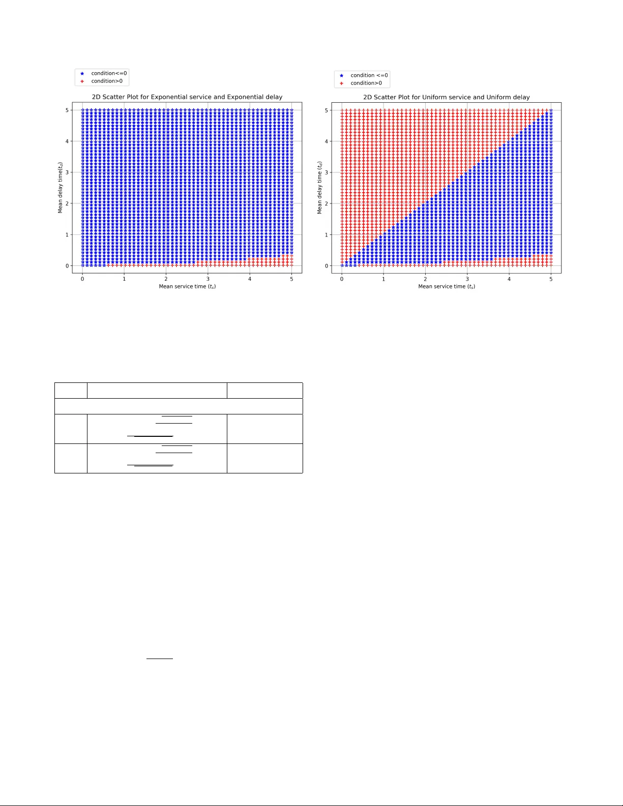
Authors: Padma Priyanka, Avhishek Chatterjee, Sheetal Kalyani
1 Maximizing Qubit Throughput under Buf fer Decoherence and V ariability in Generation Padma Priyanka, A vhishek Chatterjee, and Sheetal Kalyani Abstract —Quantum communication networks r equire trans- mission of high-fidelity , uncoded qubits for applications such as entanglement distribution and quantum k ey distribution. Howev er , current implementations are constrained by limited buffer capacity and qubit decoherence, which degrades qubit quality while waiting in the buffer . A key challenge arises from the stochastic nature of qubit generation: there exists a random delay ( D ) between the initiation of a generation request and the a vailability of the qubit. This induces a fundamental trade- off—early initiation increases buffer waiting time and hence decoherence, whereas delayed initiation leads to server idling and reduced throughput. W e model this system as an admission control problem in a finite-buffer queue, where the reward associated with each job is a decreasing function of its sojour n time. W e derive analytical conditions under which a simple “no-lag” policy—wher e a new qubit is generated immediately upon the av ailability of buffer space—is optimal. T o addr ess scenarios with unknown system parameters, we further de velop a Bayesian learning framework that adaptiv ely optimizes the admission policy . In addition to quantum communication systems, the proposed model is appli- cable to delay-sensiti ve IoT sensing and service systems. Index T erms —Quantum Communication; Qubit Decoherence; I . I N T R O D U C T I O N Quantum communication networks are rapidly gaining prominence through practical deployments. A crucial step in many of these practical quantum communication systems is the transmission of high-quality uncoded qubits to an intended destination. For the quantum internet, it is important to generate entangled pairs rapidly and send one qubit from each pair to the intended destination [1], [2]. For quan- tum key distribution, transmitting specially designed (and randomly chosen) high-quality qubits at a high rate is a crucial step [1], [2]. In some of these applications, quantum error-correcting codes may improve performance. Howe ver , current technologies do not allo w for sophisticated quantum encoding and decoding, as this w ould require a miniature f ault- tolerant quantum computer , which is not realizable at present. Hence, in current systems, uncoded qubits are transmitted for entanglement sharing and ke y distribution [2]–[4]. In [5]–[7], the classical Shannon capacity of such systems with qubit decoherence in the transmission b uffer w as studied. Motiv ated by the constraints of current quantum technologies, in this paper the metric of interest is the rate of transmission of uncoded qubits at a pre-specified acceptable quality . In This work was supported in parts by ANRF India through grant CRG/2023/005345. The authors are with the Department of Electrical Engineering, Indian Institute of T echnology Madras, Chennai, India. addition to uncoded qubits, this work considers another prac- tical issue faced by current quantum communication systems: transmission buf fers have small capacity ( ≤ 2 ). This is due to the fact that most quantum communication systems rely on single-photon transmission, and current photonic b uffers hav e limited capacity [8], [9]. W e consider the case where at most one qubit can wait in the transmission buf fer while the qubit generated immedi- ately before it is being transmitted. The decision to start the generation of the ne xt qubit is taken based on the state of the transmission buf fer . This decision must balance between two undesirable cases: (i) a qubit generated too early waits for a long time in the buf fer and decoheres, and (ii) a qubit generated so late that the transmitter experiences a long idle time. These two scenarios result in poor quality and low throughput, respecti vely . Balancing between these two cases is key to maximizing the throughput of high-quality qubits, which we refer to as the re war d in the technical sections of the paper . This quantity is sometimes referred to as goodput in the literature on communication networks [10]. The mathematical formulation of the above qubit transmis- sion problem, as discussed later in Sec. II, is equiv alent to a stationary policy for admitting a job into a finite queue (buffer size 2 ), where the queue is served by a server with random service times, and an admitted job arrives after a random delay from the time of its admission by the policy . The objective in this scenario is to maximize the av erage rew ard across jobs, where the rew ard for a job is a decreasing function of its sojourn time, i.e., the total time the job spends in the system after arri val. Interestingly , as discussed in Sec. II, the same mathematical formulation is also useful in delay-constrained sensing and communication for memory-constrained IoT de vices. It also turns out that a similar formulation closely represents the prob- lem of serving a large number of customers with reasonable service quality in certain online and offline service sectors. In general, understanding the trade-of f between the quality of qubits and their throughput, and choosing the appropriate operating point, is crucial in many quantum communication scenarios; hence, it is a topic of activ e research [3], [4], [11]– [13]. A. Main Contributions The first contribution of this work is the formulation of the abov e qubit generation problem as an admission (or calling) problem in a finite-b uffer queue. The goal is to maximize the av erage rew ard of the finite-buf fer queueing system, where 2 each job accrues a rew ard that is a general function of its sojourn time. This formulation is sho wn to be useful in IoT and delay-sensitiv e communications, as well as in certain service platforms. Building on this formulation, we analytically characterize the region of distributions and parameters for which the simplest implementable policy is optimal: admit (or call) a job as soon as the job in service departs. Since IoT sensors have limited computational capability , and integrating complicated semiconductor electronics with optical buf fers in quantum communication systems is challenging, the abo ve simple pol- icy is highly desirable. Finally , we de velop a Bayesian learning framework that enables policy optimization without prior knowledge of arri val or service time distributions, thereby relaxing the classical assumption of full distributional information. The Bayesian learning framew ork is adaptiv e in nature and therefore can also handle mean drift and mean shift, which are important practical issues in quantum communications [14], [15]. B. Organization The remainder of this paper is organized as follo ws. Section II describes the system model and preliminaries. Section III presents the analytical framework and theoretical results. Section IV reports the simulation results. Section V concludes the paper and discusses the directions for future work. I I . S Y S T E M M O D E L In a traditional queuing system, a server serves jobs sequen- tially in their order of arriv al. While the server serves a job the jobs which arriv ed behind it wait in a queue, which can hold a large number of jobs. Here, motiv ated by the applications discussed above, we consider the follo wing server and queue system. The service times of the jobs are i.i.d. { S i } . There is an infinite reservoir of jobs from which the queue calls jobs. Howe ver , there are random i.i.d. delays { D i } between calling (or admitting) a job and its arriv al to the queue. At most two jobs can be in the queue at any point of time, with one of them in service. The problem in hand is to decide when the next job should be called after the waiting job goes into service. This decision should be chosen to optimize a long-term average reward of the system, which depends on the sojourn times of the jobs. For most practical queuing systems, stationary policies are sought due to their ease of implementation and good performance [16], [17]. The most natural class of policies for this setting is the choice of a lag ∆ , between the waiting job entering service and calling the next job into the b uffer . In this work, we consider policies for which ∆ is chosen deterministically . Let { T i } be the respecti ve sojourn times of jobs i = 1 , 2 , . . . , under a particular polic y taken by the queue for calling jobs. Sojourn time of a job is its service time plus the time spent waiting in the queue. For most practical queuing systems, stationary policies are sought due to their ease of implementation. A stationary policy leads to a stationary and ergodic queue ev olution and hence, the rate of processing of jobs is well defined and so is the stationary distribution of sojourn times. W e denote them by λ and T , respecti vely . For job i , the system earns a rew ard f ( T i ) , where f is a non-negati ve and non-increasing function of the sojourn time. Let N ( t ) be the total number of jobs served by the queue up to time t . The central problem of this paper is the following. max ∆ ≥ 0 lim t →∞ 1 t N ( t ) X i =1 f ( T i ) . The above limit is almost surely deterministic and finite for all ∆ ≥ 0 , since the queueing system is stable. Though the abov e problem is quite simple to state, related problems in the simpler case with infinite buf fer, are known to be intractable [18]. Hence, a complete analytical or algorithmic solution for obtaining the optimal ∆ in the finite buf fer case is intractable. Here, we take an important first step by analytically charac- terizing practically verifiable conditions under which a simple policy of no lag, i.e. ∆ = 0 , is optimal. This intuiti ve polic y of calling the ne xt jobs as soon as the pre vious job enters service is easy to implement and hence, is the natural choice in many practical systems. Our analytical result giv es conditions when this intuitiv e policy is indeed the best policy . Later , we propose a Bayesian learning scheme that chooses ∆ adapti vely by learning from the past re wards. The abo ve limit can be re written as a simple expression in terms of expectation with respect to the stationary distribution of the queue. Clearly , for any finite ∆ , N ( t ) → ∞ almost surely , if S and D have proper distributions (i.e., no mass at infinity). Thus, the limit lim t →∞ 1 t P N ( t ) i =1 f ( T i ) can be rewritten as lim t →∞ N ( t ) t 1 N ( t ) P N ( t ) i =1 f ( T i ) . For any finite ∆ , since the system is stationary and er godic [16], [17], [19], N ( t ) t → λ and 1 N ( t ) P N ( t ) i =1 f ( T i ) → E [ f ( T )] , almost surely . Here, the expectation is with respect to the stationary distribution of the sojourn time. Thus, the above problem can be reformulated as: find the ∆ ≥ 0 that maximizes the expected re ward, G = λ E [ f ( T )] , which is equal to the long-term average reward. As discussed in Sec. I, though quantum communication is the main moti vation of the abov e problem, it has direct applica- tions in multiple other domains. Here, we first discuss how the abov e formulation is natural for the quantum communication scenarios discussed in Sec. I. Follo wed by this we discuss how the problem emerges in applications like IoT and delay sensitiv e communication. Finally , we discuss its application in service sectors. Application in Quantum Communication: Decoherence of uncoded qubits in the transmission b uffer , and how that leads to a tradeoff between high qubit transmission rate and quality of qubits hav e been discussed in Sec. I. This tradeoff naturally leads to a natural metric: throughput or rate of transmission of qubits that are above a certain quality lev el (a.k.a. quantum state fidelity [1]). In the well known erasure and depolarizing noise models for qubit decoherence [1], qubits remain uncorrupted with a probability 1 − p and with probability p it degenerates into a useless quantum state (erasure or maximally mixed state). The probability of a qubit being uncorrupted, 1 − p , 3 decreases with the time a qubit spends in contact with the en vironment (sojourn time in the transmission buf fer or queue, in our case) and is captured by a non-negati ve and non- increasing function f ( · ) of its sojourn time. Thus, the ex- pected number of uncorrupted qubits transmitted per unit is lim t →∞ 1 t E P N ( t ) i =1 f ( T i ) , which, by Fubini-T onelli theorem [20] is E h lim t →∞ 1 t P N ( t ) i =1 f ( T i ) i = lim t →∞ 1 t P N ( t ) i =1 f ( T i ) . Since the last limit is almost surely deterministic for any stationary policy for generating qubits based on the buf fer state. Applications in IoT and Delay Sensitive Communications: W ireless IoTs are often used for monitoring critical processes. Sensors in IoT devices sense the en vironment and share the measurements as packets over a multiple access wireless channel, which is closely modeled as a serv er with random service times. If the sensor sends samples or measurements frequently , the receiver or the decision center will hav e many highly delayed measurements, resulting in delay in decision making. On the other hand, too fe w samples will also lead to delay in decision making. A tradeof f would be send measurements or packets as frequently as possible while ensuring a tolerable delay [21]–[23]. Mathematically , if { T i } are delays of the samples, the goal is to maximize the number of samples delivered per unit time with low delay , i.e., max E { T i ,V i } 1 t P N ( t ) i =1 1( T i ≤ V i ) . Here, N ( t ) is the number of samples deliv ered by t and V i is the threshold (possibly random) by which sample or packet i must be deliv ered. In general, E V i 1( T i ≤ V i ) would be f ( T i ) , where f depends on the distribution of V i . Thus, the whole expression is equiv alent to N ( t ) t · 1 N ( t ) E { T i } P N ( t ) i =1 f ( T i ) . Also, since in many applications IoT sensors are frugal, the b uffer for holding samples or packets before transmission is often small ( ≪ 10 ) [24]. Thus, the queueing problem discussed above is indeed the right problem to consider in this setting as well. Application in Customer Service: Consider a real-time scenario where a hospital or restaurant’ s customer waiting room has limited capacity and can accommodate only one or two customers maximum at a time. If customers experience longer waiting times, their satisf action decreases, which results in negati ve online feedback or revie w . The service portal’ s effecti ve re venue for a customer is a combination of service charge and the customer’ s satisfaction. This effecti ve rev enue can be modeled as a function f ( T ) , where T represents the total time in the system. This function f is naturally non- increasing in T and can be of exponential or polynomial form [25]–[28], depending on the application. The objectiv e here would be to maximize the total expected effecti ve re venue per unit time, which is again λ E [ f ( T )] . I I I . A N A L Y T I C A L A P P R O AC H W e first consider a general non-increasing and non-negati ve function f ( T ) . Later we consider f ( T ) = exp( − κT ) moti- vated by the application in quantum communications [1], [3], [6]. W e also consider f ( T ) = 1 ( T +1) γ inspired by the IoT sensing and customer service applications [21], [25]–[28]. The sojourn time T of a typical job in the system is its waiting time W plus its service time S . The waiting time W aiting T ime ∆ Delay t = t 2 2 nd job arrives t = t 2 + w 2 nd job goes for service t = t 2 + w + ∆ Call 3 rd job t = t 2 + w + ∆ + d 3 rd job arrives Fig. 1. Calculation of inter-arri val time W depends on the service of the job before it, the lag ∆ in calling the current job and the delay D in its arriv al. Here, we assume the lag is deterministic. Thus, despite the service, delay and lag being independent, the sojourn times of the jobs are correlated. Here our interest is in the quantity λ E [ f ( T )] , which is well defined and finite. First, we understand the relation between waiting time W of the current job and the service time of the previous job, which we denote by S − 1 . This would allow us to e valuate both E [ f ( T )] and λ and thus obtain G . Let the interarri val time between two jobs be denoted by IA T. Then, by elementary rene wal theorem [19], the rate of arriv al of jobs λ = 1 E [ IA T ] . A job is called ∆ time after the previous job has gone into service and it arri ves D time after calling. Thus, IA T is nothing but the sum of the waiting time of the pre vious job, ∆ and D . This is shown in Fig. 1. Thus, E [ IA T ] = ∆ + E [ D ] + E [ W ] . Here, the last term is the expected waiting time of the previous job, which, by stationarity , is equal to E [ W ] . Clearly , T = W + S and W is independent of S . So, E [ f ( T )] = E [ f ( W + S )] . For obtaining E [ W ] , note that the called job reaches ∆ + D time after calling and the job in service (previous job) takes S − 1 time to get served. Thus, if the called job reaches before the previous job is served, it has to wait for the remaining service to be completed. But, if it reaches after the service has been completed, it does not wait at all. Hence, W = max( S − 1 − ∆ − D, 0) . Thus, for a deterministically chosen lag, the expression for the general rew ard becomes G = E [ f ( W + S )] ∆ + E [ D ] + E [ W ] (1) A. General re war d with general function f(T) for general service distrib ution and g eneral delay distribution T o determine the optimal lag, we start with the general service distribution and the general delay distribution with well-defined e xponential moments for general function f ( T ) . Theorem 1. The general r ewar d function G associated with the proposed queueing system, characterized by general ser- vice and a gener al delay distrib ution, with a g eneral function f and a deterministically chosen lag, attains its global maximum at ∆ = 0 , if the following conditions holds: E [ D + S + 1] p E [( f ′ ( S )) 2 ] E [ f ( S + S − 1 )] ≤ 1 p P ( S − 1 − D > 0) − p P ( S − 1 − D > 0) 4 Pr oof. The re ward function is given by G = E [ f ( S + W )] ∆ + E [ D ] + E [ W ] (2) An important intermediate result that we use in this setting is the follo wing lemma, which is pro ved later . d E [ W ] d ∆ = − P ( S − D > ∆) T o maximize the rew ard function over ∆ , the deriv ativ e of rew ard function w .r .t ∆ is giv en by dG d ∆ = E f ′ ( S + W ) dW d ∆ (∆ + E [ D ] + E [ W ]) (∆ + E [ D ] + E [ W ]) 2 − 1 + d E [ W ] d ∆ E [ f ( S + W )] (∆ + E [ D ] + E [ W ]) 2 (3) If ( dG d ∆ < 0 , ∀ ∆ ≥ 0) ⇐ ⇒ ( Numerator of equation (3) < 0 , ∀ ∆ ≥ 0) , then optimal ∆ = 0 . If f(x) is a decreasing function, then f ′ ( x ) < 0 and | f ′ ( x ) | decreases as x increases. Therefore, f ′ ( S + W ) dW d ∆ ≤ | f ′ ( S ) || 1 ( S − 1 − D > ∆) | The first term in the numerator of the equation (3) is upper bounded by (∆ + E [ D ] + E [ S ]) E [ | f ′ ( S ) || 1 ( S − 1 − D > ∆)] ≤ (∆ + E [ D ] + E [ S ]) p E [( f ′ ( S )) 2 ] p E [ 1 ( S − 1 − D > ∆)] (Cauchy–Schwarz inequality) ≤ (∆ + E [ D ] + E [ S ]) p E [( f ′ ( S )) 2 ] p P ( S − 1 − D > ∆) (Lemma 1) ≤ E [ D + S ] p E [( f ′ ( S )) 2 ] P ( S − 1 − D > ∆) + p ∆ 2 E [( f ′ ( S )) 2 ] P ( S − 1 − D > ∆) ≤ E [ D + S ] p E [( f ′ ( S )) 2 ] P ( S − 1 − D > 0) + p E [( f ′ ( S )) 2 ] P ( S − 1 − D > 0) ≤ E [ D + S + 1] p E [( f ′ ( S )) 2 ] P ( S − 1 − D > 0) For ∆ ≤ 1 , we hav e ∆ 2 P ( S − 1 − D > ∆) ≤ P ( S − 1 − D > ∆) ≤ P ( S − 1 − D > 0) . For ∆ > 1 we assumed ∆ 2 P ( S − 1 − D > ∆) is decreasing with ∆ . The second term in the numerator of the equation (3) is P ( S − 1 − D ≤ ∆) E [ f ( S + W )] ≥ P ( S − 1 − D ≤ 0) E [ f ( S + max( S − 1 − D , 0))] (Both terms attain their minimum when ∆ = 0 ) ≥ P ( S − 1 − D ≤ 0) E [ f ( S + S − 1 )] , ∀ ∆ Therefore ∆ = 0 is optimal if E [ D + S + 1] p E [( f ′ ( S )) 2 ] P ( S − 1 − D > 0) ≤ P ( S − 1 − D ≤ 0) E [ f ( S + S − 1 )] = ⇒ E [ D + S + 1] p E [( f ′ ( S )) 2 ] E [ f ( S + S − 1 )] ≤ 1 p P ( S − 1 − D > 0) − p P ( S − 1 − D > 0) Lemma 1. d E [ W ] d ∆ = − P ( S − D > ∆) (4) Pr oof. W aiting time W is gi ven by W = max( S − 1 − ∆ − D , 0) (5) dW d ∆ = − 1 ( S − 1 − D > ∆) + α 1 ( S − 1 − D = ∆) where − 1 ≤ α ≤ 0 . The second term is zero if S − 1 and D are continuos random v ariables. Let U = S − 1 − D , then max( U − ∆ , 0) = ( U − ∆ if U > ∆ 0 elseif U ≤ ∆ d d ∆ max( U − ∆ , 0) = ( − 1 if U > ∆ 0 elseif U ≤ ∆ = ⇒ dW d ∆ = − 1 ( S − 1 − D > ∆) Therefore, d E [ W ] d ∆ = d d ∆ E [max( S − 1 − ∆ − D , 0)] = E [ d d ∆ max( S − 1 − ∆ − D , 0)] = E [ d d ∆ max( U − ∆ , 0)] = Z d d ∆ max( U − ∆ , 0) f U ( u ) du = Z U > ∆ − 1 .f U ( u ) du = − Z U > ∆ f U ( u ) du = − P ( S − 1 − D > ∆) = − P ( S − D > ∆) (Since the system is stationary) The condition deri ved in Theorem 1 is a sufficient condition for the optimal lag to be ∆ = 0 , and it holds for any function f . Howe ver , in practice, f mostly ha ve exponential or polynomial form [1], [5]–[7], [29]. Therefore, we first consider the exponential function f , which is practically moti vated by applications in quantum communication, where decoherence ef fects naturally lead to exponential penalties in the sojourn time [1], [5], [6]. W e also study a polynomial re ward function, motiv ated by IoT 5 sensing and customer service applications in which perfor- mance metrics are closely related to the moments of delay [21], [25]–[28]. For both exponential and polynomial reward functions, the resulting sufficient conditions admit insightful interpretations. In particular, the exponential rew ard function corresponds to moment generating functions of the sojourn time, while the polynomial reward function is directly related to ne gati ve moments. B. General r ewar d with exponential function f(T) for general service distrib ution and g eneral delay distribution Here, we consider f ( T ) = exp( − κT ) and our interest is in the quantity λ E [exp( − κT )] , which is well defined and finite. So, E [exp( − κT )] = E [exp( − κW )] E [exp( − κS )] . Henceforth, for any random v ariable X and any real number a , we shall denote E [exp( aX )] by M X ( a ) , whenev er it is well defined. Note that M W ( − κ ) and M S ( − κ ) are well defined and finite since W and S are non-negati ve. Thus, G = M W ( − κ ) M S ( − κ ) ∆ + E [ D ] + E [ W ] . From the knowledge of the distribution of S , M S ( − κ ) can be obtained. For obtaining M W ( − κ ) ,the waiting time is W = max( S − 1 − ∆ − D , 0) , which implies M W ( − κ ) ≤ min( M S ( − κ ) M ∆ ( κ ) M D ( κ ) , 1) by Jensen’ s inequality and independence of S − 1 , ∆ and D . The term M S ( − κ ) replaces M S − 1 ( − κ ) in the above expres- sion since for a stationary system they are the same. Since the lag ∆ is chosen deterministically , the term M ∆ ( κ ) = e κ ∆ . This implies that the follo wing expression is a surrogate for G that upper-bounds it. G sur = M S ( − κ ) min( M S ( − κ ) e κ ∆ M D ( κ ) , 1) ∆ + E [ D ] + E [ W ] (6) Later , we shall discuss the utility of this surrogate upper bound for e xponential f . Corollary 1. The gener al r ewar d function G associated with the pr oposed queueing system c haracterized by general service and a general delay distribution for the exponential function f ( x ) = exp( − κx ) and deterministically chosen lag, attains its global maximum at ∆ = 0 , if it satisfies the condition κ E [ D + S + 1] p M S ( − 2 κ ) ( M S ( − κ )) 2 ≤ 1 p P ( S − 1 − D > 0) − p P ( S − 1 − D > 0) Pr oof. Let f ( x ) = exp( − κx ) . Then, E [( f ( S )] = E [ e − κS ] = M S ( − κ ) , E [( f ′ ( S )) 2 ] = E [ e − 2 κS ] = M S ( − 2 κ ) . By substi- tuting these in to the general sufficient condition for optimal ∆ = 0 we get the following κ E [ D + S + 1] p M S ( − 2 κ ) ( M S ( − κ )) 2 ≤ 1 p P ( S − 1 − D > 0) − p P ( S − 1 − D > 0) Corollary 2. The gener al r ewar d function G associated with the pr oposed queueing system char acterized by gener al ser- vice and gener al delay distrib ution for polynomial function f ( x ) = 1 ( x +1) γ and deterministically chosen lag, attains its global maximum at ∆ = 0 , if it satisfies the condition γ E [ D + S + 1] p E [( S + 1) − 2 γ − 2 ] E [( S + S − 1 + 1) − γ ] ≤ 1 p P ( S − 1 − D > 0) − p P ( S − 1 − D > 0) Pr oof. Let f ( x ) = 1 ( x +1) γ . Then, E [( f ( S )] = E [( S + 1) − γ ] , E [( f ′ ( S )) 2 ] = γ 2 E [( S + 1) − 2 γ − 2 ] . By substituting these in to the general suf ficient condition for optimal ∆ = 0 we get the following γ E [ D + S + 1] p E [( S + 1) − 2 γ − 2 ] E [( S + S − 1 + 1) − γ ] ≤ 1 p P ( S − 1 − D > 0) − p P ( S − 1 − D > 0) If we consider optimizing the surrogate rew ard function for the exponential function, which is an upper bound, we get a set of simpler conditions that are easier to check. Hence, we discuss them below . Theorem 2. The surr ogate r ewar d function G sur associated with the pr oposed queueing system char acterized by general service and a g eneral delay distrib ution for exponential func- tion f ( x ) = exp( − κx ) and deterministically chosen lag, attains its global maximum at ∆ = 0 , if one of the following conditions holds: 1) M S ( − κ ) M D ( κ ) ≥ 1 2) 1 κ ln 1 M D ( κ ) M S ( − κ ) + E [ D ] + [ E [ W ]] ∆=0 < 1 κ P ( D > S ) The detailed proof of Theorem 2 is given in Appendix A. The abov e-deriv ed results establish the conditions under which ∆ = 0 is the optimal choice to attain a maximum v alue of the reward function. The optimal value of ∆ for different conditions is giv en in T able I. Ho wev er , it is not clear what fraction of distributions and their parameters satisfy these conditions. T o gain a better understanding of this, we visualize the parameter space for the exponential function by plotting the regions where the optimality condition in T able I holds. The plotted regions are colour-coded to represent dif ferent ranges of parameter values and their corresponding effects on the system’ s behaviour . This helps to identify and interpret the boundaries of the parameter space where ∆ = 0 is optimal, providing a clearer insight into the practical applicability of the theoretical results. The 2D scatter plot of the reward function against service and delay time parameters is plotted in Fig. 2 for different service and delay distributions to identify the region that satisfies the desired conditions given in T able I. If the service and delay parameters are chosen within the blue region which 6 (a) (b) Fig. 2. 2D scatter plot of the reward function v ersus service and delay time parameters. (a) Exponential service and exponential delay distrib ution. (b) Uniform service and uniform delay distribution T ABLE I G E N E R A L D I S T R I B U T I O N C O N D I T I O N TO FI N D O P T I M A L ∆ S.No Condition Optimal ∆ ∆ is chosen deterministically for any general function f 1 E [ D + S + 1] √ E [( f ′ ( S )) 2 ] E [ f ( S + S − 1 )] − 1 − P ( S − 1 − D> 0) √ P ( S − 1 − D> 0) ≤ 0 ∆ = 0 2 E [ D + S + 1] √ E [( f ′ ( S )) 2 ] E [ f ( S + S − 1 )] − 1 − P ( S − 1 − D> 0) √ P ( S − 1 − D> 0) > 0 Depends on κ , service and delay parameter satisfies condition 1 gi ven in T able I, then ∆ = 0 is the optimal choice of the lag. If the parameters are chosen in the red region which does not satisfy Condition 1, the optimal lag value depends on κ , service, and delay parameters. C. Grid sear ch as a benchmark A grid search approach can be used to empirically determine the optimal lag ∆ , ev en when the service and delay time distributions are unknown. In this approach, the queue is simulated by generating n service and delay samples with the mean service time t s and the mean delay time t d from the unknown underlying service and delay distribution. For each value of ∆ , the reward E [ f ( T )] E [ I AT ] is estimated from the simulated data. The grid search identifies the optimal calling time ∆ sim that has a maximum simulated re ward G sim . The grid search can only serve as a benchmark since one will not have access to the large set of samples from the activ e queue. The Bayesian learning method of fers a principled alternativ e frame work for this problem by incorporating prior information and sequentially updating posterior beliefs based on observ ed data. D. Bayesian Estimation of optimal ∆ In Section II-A, an optimal job-calling policy was proposed for general service and delay distributions that maximizes the rew ard function. The lag is deterministic, and we showed in Theorems 1,2 that under certain conditions, ∆ = 0 is optimal lag time. Here, we are trying to find the optimal ∆ for cases that do not fall under these Theorems. In the general case, mathematically , it is quite hard to get a closed-form expression for the reward function in order to find the optimal lag. For example, when the service and delay distributions are uniform or exponential, expressions for the re- ward function and the corresponding conditions can be derived to determine the optimal v alue of ∆ . In contrast, obtaining such expressions becomes mathematically intractable when the distrib utions follo w a truncated normal form. The natural question that arises is, if we cannot theoretically determine the optimal lag time, can we learn it using Bayesian methodology? In practice, the distrib utions of service and delay time may not be known. Hence, the optimal calling distribution has to be learned over time. T o address this, we estimate the optimal lag using a para- metric Bayesian learning approach. In this approach, the lag ∆ is modelled as a random variable with a distribution character- ized by parameter θ . The conjugate prior distribution, namely the gamma distribution for the parameter of the estimated lag is maintained and updated for ev ery data sample, as samples arriv e. The Bayesian approach relies on conjugate prior distribu- tions to ensure analytical tractability . Howe ver , for heavy- tailed distributions, such as the Generalized Pareto Distribu- tion (GPD) and the Hyper-Exponential Distribution (HED), conjugate priors are complex. So, we model the optimal lag distribution using an exponential distrib ution [30] since 7 Algorithm 1 Proposed Algorithm Initialization α 0 = 1 , β 0 = 1 , ∀ j = 1 , 2 , ..., N . Server State = S, Server busy = b , Server idle = i . for j= 1,2,...,N samples do Draw a sample ˆ θ ∼ G ( α j − 1 , β j − 1 ) t = 1 ˆ θ if j = 1 and S j = i then β j ← β j − 1 + t α j ← α j − 1 + ϵ idle else if j = 1 and S j = b then β j ← β j − 1 + t α j ← α j − 1 + ϵ busy else if S j = i and S j − 1 = i then β j ← β j − 1 + t α j ← α j − 1 + ϵ idle else if S j = b and S j − 1 = b then β j ← β j − 1 + t α j ← α j − 1 + ϵ busy end if end if end f or 1) It is non-negati ve. 2) It is a maximum entropy distribution among all continu- ous PDFs defined on [0, ∆ ]. With a fixed specified mean, it is the least informative distribution. 3) Its conjugate prior is simple, i.e., the gamma distrib ution. The lag is assumed to be a sample from an exponential distribution with parameter θ i.e., ∆ ∼ E xp ( θ ) = θ e − θt The mean of the distribution is 1 /θ , which corresponds to the mean lag time. Therefore, to determine the lag time(t), we consider the in verse of the sample obtained from the prior distribution. Physically , 1 /θ signifies the mean time duration to call the next job . As we w ould like to learn this value and use it as a proxy for optimal lag time. The conjugate Gamma prior for θ is parameterized by α and β , i.e, θ ∼ G ( α, β ) . p ( θ ) = β α Γ( α ) θ α − 1 e − β θ 1) W orking of Algorithm: Our objective is to estimate the optimal lag time to call the next job . The queue is simulated by drawing a sample from the service and delay distribution. The lag time is found by drawing a sample ˆ θ from the conjugate posterior distrib ution and taking the in verse. The motiv ation for sampling from the Gamma posterior distrib ution, rather than using its mean α/β , is to enable exploration of both smaller and larger lag values, thereby increasing the likelihood of conv erging to the optimal lag duration. As the number of observations increases, the parameters of the distribution are updated, and the v ariance of the Gamma distrib ution decreases. The posterior distribution of θ is gi ven by p ( θ | x ) ∝ β α Γ( α ) θ α − 1 e − β θ θ e − θx ∝ θ α +1 − 1 e − ( β + x ) θ p ( θ | x ) ∼ Γ( α + 1 , β + x ) The posterior distribution seen ov er n samples is giv en by p ( θ | x 1 , x 2 , ..., x n ) ∼ Γ( α + n 0 , β + n X j =1 x j ) where n 0 is the number of optimal lag time periods. As the number of observed lag samples x j increases, the posterior distribution p ( θ | x 1 , x 2 , ..., x n ) concentrates around the maxi- mum lik elihood estimate. The hyperparameters α and β are updated when both the current and previous server states are identical, i.e., both idle or both busy . If one state is idle and the other is b usy , the server is considered to be in steady state, and no update is performed. The parameter α tracks the number of optimal lag periods that have been elapsed for the chosen lag sample 1/ ˆ θ . W e assume ϵ idle and ϵ busy optimal periods ha ve passed if both the present and previous server status are idle and busy respectiv ely . The parameters ϵ idle and ϵ busy determine ho w the conjugate posterior parameters are updated in response to recent server activity . The lag time is in versely proportional to the α , for each lag sample α is updated depending on the server status. If the present and previous server state is idle, this indicates that a decrease in lag time is possible due to server av ailability which means that the mean lag time can be decreased, α is increased by ϵ idle . Similarly , if the present and previous server states are busy , the mean lag time should be increased, α is increased by ϵ busy . This action serves to increase the lag time, likely as a response to high server load. The parameter β is updated by observed lag period if both present and previous server status are either idle or busy . Therefore after observing n samples, α is updated by n 0 , which gi ves number of optimal lag periods and β gives the total duration of observ ed optimal lag period. By continuously updating the parameters with each ne w sample, we arrive at an appropriate lag time distribution and the posterior mean con ver ges to the optimal mean lag time. Further , when the service and delay distributions themselves change ov er time, and the change is unknown, the Bayesian method can adapt to the change. In such non-stationary settings, a Bayesian approach can adapt more naturally to these changes by continuously updat- ing the posterior as new observ ations arrive, allowing it to track distrib utional shifts more effecti vely . I V . S I M U L A T I O N R E S U LTS In this section, we present simulation results of the grid search and Bayesian estimation methods for estimating the optimal lag time that maximizes the reward function. In all simulations, the reward is computed using the exponential form f ( T ) = exp( − κT ) due to its mathematical tractability . 8 Fig. 3. Comparison of Grid search estimated rew ard and the theoretical surrogate rew ard for different service and delay distributions with t s = 1 , t d = 0 . 33 T ABLE II C O M P A R I S O N OF B AY E S I A N E S T I M AT E D RE W A R D A N D TH E T H E O R E T I C A L S U R R O G AT E R E W A R D F O R DI FF E R E N T S E RV I C E A N D D E L AY D I S T R I B U T I O N S t s t d G sur G be G tb Case A: Exponential service and Exponential delay distribution 1 0.33 0.90910 0.8969 0.8888 0.5 0.1667 1.8308 1.7946 1.7779 Case B: Exponential service and Uniform delay distribution 1 0.33 0.9657 0.9628 0.9527 0.5 0.1667 1.9485 1.9359 1.9161 Case C: Uniform service and Uniform delay distribution 1 0.33 1.9139 1.8908 1.8934 0.5 0.1667 3.8410 3.7841 3.7506 Case D: Uniform service and Exponential delay distribution 1 0.33 1.6455 1.6451 1.6321 0.5 0.1667 3.2914 3.2816 3.2545 Case E: Exponential service and T runcated Normal delay distribution 1 0.33 - 0.7497 - 0.5 0.1667 - 1.2584 - Case F: T runcated Normal service and T runcated Normal delay distribution 1 0.33 - 0.7419 - 0.5 0.1667 - 1.0148 - A. Grid sear ch results In Fig. 3, the grid search estimated rew ard is compared with the theoretical surrogate re ward for t s = 1 , t d = 0 . 33 . W e observed that the estimated rew ard curve for the grid search matches the theoretical surrogate reward for a chosen service and the delay time. Therefore, all the abov e observations reinforce our theoretical results. B. Bayesian estimation r esults The optimal lag is estimated using the proposed Bayesian approach by modelling the queue with exponential or general service-time and delay-time distributions. For the general case, uniform, exponential, and truncated normal distributions are Fig. 4. Comparision of Bayesian estimated rew ard and theoretical surrogate rew ard for different service and delay distributions with t s = 1 , t d = 0 . 33 considered. In the proposed algorithm 1, the hyperparameters α and β are adapti vely updated depending on the server av ailability . The parameters ϵ idle , ϵ busy play an important role in updating the conjugate posterior distribution parameters. T o find an appropriate value for ϵ idle , ϵ busy , extensi ve e valuation studies are done and found that ϵ idle = 3 , ϵ busy = 1 works well. In all the cases, the queue is simulated for 50000 samples with ϵ idle = 3 , ϵ busy = 1 and the optimal lag is estimated using Bayesian method. Once the Bayesian algorithm has con ver ged, the optimal lag is determined. Due to inherent randomness in each run, the estimated mean lag may v ary across trials. Hence, the reward function is ev aluated to enable comparison with the surrogate theoretical rew ard. The reward function E [exp( − κT )] E [ I AT ] , is calculated using last 5000 samples. In Fig. 4 and T able II, for different service and delay distribution the Bayesian estimated reward G be is compared with the theoretical surrogate re ward G sur and observ ed G be is approximately equal to G sur . In Fig. 4, it is observed that the Bayesian estimated reward rapidly conv erges to the theoretical surrogate rew ard within the initial few samples and subsequently adapts to changes in the underlying distribution. The theoretical surrogate reward v alue G tb is calculated for the Bayesian estimated lag time and compared it with true theoretical surrogate re ward G sur . It was observed that G tb and G sur values were very close, confirming that Bayesian estimation is effecti ve for finding the optimal calling time. In T able II, for cases A to D, the system is stationary and we could derive the theoretical expressions for the rew ard function. In T able II, for cases E,F the system is stationary , but obtaining a closed form theoretical expressions for the surrogate rew ard function is very difficult for exponential service and truncated normal delay distribution and truncated normal service and delay distributions. In these cases, we estimated the rew ard function G be using Bayesian methods and observed the rew ard value is close to the grid search simulated reward G sim . 1) Mean shift of service and delay distribution: W e now consider scenarios in which the system’ s characteristics vary 9 (a) (b) Fig. 5. Mean-shift comparison of Bayesian estimated reward and the theoretical surrogate re ward for exponential service and e xponential delay distributions. (a) Gradual change in mean of service and delay distribution. (b) Abrupt change in mean of service and delay distribution. ov er time, either gradually or abruptly . In the proposed theory and grid search we take expectation to calculate the rew ard function under the assumption of a stationary system. The proposed algorithm employs sequential Bayesian esti- mation to enable continuous learning, allo wing it to adapt to changes in the parameters of the service and delay distributions by updating the posterior distribution, without discarding prior observations. In Fig. 5a, the mean service and delay times are gradu- ally changed linearly and the Bayesian estimated re ward is calculated using the sliding window method. In Fig. 5b, the mean service and delay times are changed for e very 10000 samples and the Bayesian estimated reward is calculated with- out considering the transient phase. In Fig. 5, for the gradual and abrupt change in the mean service and delay distribution, the Bayesian estimated rew ard G be is approximately equal to the theoretical surrogate reward G sur . In non-stationary cases, for each pair of mean service and delay times ( t s , t d ) respectiv ely , the theoretical re ward function is e valuated o ver different lag-time samples, and the maximum reward is chosen as the theoretical surrogate rew ard. In contrast, the Bayesian approach does not require prior knowledge of changes in mean service and delay times, it adaptiv ely learns and estimates the rew ard from the observed data. Therefore, the proposed algorithm exhibits robustness by effecti vely adapting to both rapid and gradual changes in the service and delay parameters through continuous posterior updates enabled by sequential Bayesian estimation. V . C O N C L U S I O N This paper addresses the practical challenge of maximiz- ing the throughput of high-quality qubits in the presence of decoherence and limited transmission buffer capacity . By formulating the qubit generation process as an admission control problem for a finite-b uf fer queue, we develop a rigorous analytical framework that characterizes the trade- off between qubit fidelity and transmission rate. W e deriv e verifiable conditions under which a simple and implementable zero-lag admission policy is optimal. T o account for the limitations of static analytical results in time-v arying en vironments [14], [15], we further propose a parametric Bayesian learning algorithm that enables the system to adaptiv ely learn optimal generation times without prior kno wledge of the underlying distrib utions. The proposed frame work provides actionable insights for the design of ef ficient quantum communication systems. More- ov er , the results extend naturally to other delay-sensiti ve set- tings, including memory-constrained IoT networks and service systems. Future work will consider extensions to more general buf fer architectures and multi-user network scenarios. A P P E N D I X P R O O F O F T H E O R E M 2 Pr oof. If M S ( − κ ) M D ( κ ) ≥ 1 , the reward function is given by G = M S ( − κ ) ∆ + E [ D ] + E [ W ] (7) T o maximize the reward function o ver ∆ , the denominator should be minimized over ∆ . The deriv ativ e of denominator is giv en by 1 + d d ∆ ( E [ W ]) . By Lemma 1, the deri vati ve of the denominator, gi ven by P ( S − D ≤ ∆) , is an increasing function of ∆ . This implies that the rew ard function decreases as ∆ increases, and the re ward function G is maximum at ∆ = 0 . If M S ( − κ ) M D ( κ ) < 1 , the reward function is given by G = M S ( − κ )( M S ( − κ ) e κ ∆ M D ( κ )) ∆ + E [ D ] + E [ W ] (8) Let ∆ ∗ be the smallest ∆ for which M D ( κ ) M S ( − κ ) e κ ∆ = 1 . For ∆ > ∆ ∗ , the denominator of the reward function increases 10 with an increase in ∆ while the numerator remains the same. So, the optimal ∆ cannot be greater than ∆ ∗ . Thus, the search space is reduced to [0 , ∆ ∗ ] . Note that ∆ ∗ is gi ven by 1 κ ln 1 M S ( − κ ) M D ( κ ) (9) W e consider dG d ∆ on [0 , ∆ ∗ ] . Note that if it is negati ve on [0 , ∆ ∗ ] , the optimal choice of ∆ is 0 . After some algebraic manipulations on the deriv ativ e of G with respect to ∆ , we observe that the condition dG d ∆ < 0 is equiv alent to ∆ + E [ D ] + E [ W ] − 1 κ P ( S − D ≤ ∆) < 0 If the maximum value over the range [0 , ∆ ∗ ] of the expression in the left hand side of the above condition is less than 0 , then dG d ∆ < 0 on [0 , ∆ ∗ ] . Clearly , the expression in the left hand side of the abo ve condition has a linear increasing term in ∆ and other terms, E [ W ] and ( − P ( S − D ≤ ∆)) , that decreases with ∆ . Thus, if ∆ ∗ + E [ D ] + [ E [ W ]] ∆=0 − 1 κ P ( S − D ≤ 0) < 0 (10) then dG d ∆ < 0 on [0 , ∆ ∗ ] . Substituting the value of ∆ ∗ in equation (10), we obtain the follo wing condition: 1 κ ln( 1 M D ( κ ) M S ( − κ ) ) + E [ D ] + [ E [ W ]] ∆=0 − 1 κ P ( S − D ≤ 0) < 0 (11) Hence, when the distribution satisfies the condition given in equation (11), the rew ard function is maximized at ∆ = 0 . R E F E R E N C E S [1] M. A. Nielsen and I. L. Chuang, Quantum Computation and Quantum Information . Cambridge: Cambridge Univ ersity Press, 2000. [2] R. V . Meter, Quantum Networking . Hoboken, NJ, USA: Wiley , 2014. [3] M. Pant, H. Krovi, D. T owsley , L. T assiulas, L. Jiang, P . Basu, D. En- glund, and S. Guha, “Routing entanglement in the quantum internet, ” npj Quantum Information , vol. 5, no. 1, p. 25, 2019. [4] W . Dai, T . Peng, and M. Z. Win, “Quantum queuing delay , ” IEEE Journal on Selected Areas in Communications , vol. 38, pp. 605–618, Mar . 2020. [5] A. Chatterjee, K. Jagannathan, and P . Mandayam, “Qubits through queues: The capacity of channels with waiting time dependent errors, ” arXiv preprint arXiv:1804.00906 , 2018. [6] K. Jagannathan, A. Chatterjee, and P . Mandayam, “Qubits through queues: The capacity of channels with waiting time dependent errors, ” in 2019 National Conference on Communications (NCC) , pp. 1–6, IEEE, 2019. [7] P . Mandayam, K. Jagannathan, and A. Chatterjee, “The classical capacity of additiv e quantum queue-channels, ” IEEE Journal on Selected Areas in Information Theory , vol. 1, no. 2, pp. 432–444, 2020. [8] J.-S. T ang, Z.-Q. Zhou, Y .-T . W ang, Y .-L. Li, X. Liu, Y .-L. Hua, Y . Zou, S. W ang, D.-Y . He, G. Chen, et al. , “Storage of multiple single-photon pulses emitted from a quantum dot in a solid-state quantum memory , ” Natur e communications , vol. 6, no. 1, p. 8652, 2015. [9] S.-H. W ei, B. Jing, X.-Y . Zhang, J.-Y . Liao, H. Li, L.-X. Y ou, Z. W ang, Y . W ang, G.-W . Deng, H.-Z. Song, et al. , “Quantum storage of 1650 modes of single photons at telecom wav elength, ” npj Quantum Infor- mation , vol. 10, no. 1, p. 19, 2024. [10] J. F . Kurose, Computer networking: A top-down appr oach featuring the internet, 3/E . Pearson Education India, 2005. [11] J. Mandalapu, K. Jagannathan, and A. Thangaraj, “Capacity achieving channel codes for an erasure queue-channel, ” IEEE T ransactions on Communications , vol. 72, no. 12, pp. 7374–7386, 2024. [12] D. Chandra, A. S. Cacciapuoti, M. Caleffi, and L. Hanzo, “Direct quan- tum communications in the presence of realistic noisy entanglement, ” IEEE T ransactions on Communications , v ol. 70, no. 1, pp. 469–484, 2022. [13] A. S. Cacciapuoti, M. Calef fi, R. V . Meter, and L. Hanzo, “When entanglement meets classical communications: Quantum teleportation for the quantum internet, ” IEEE Tr ansactions on Communications , vol. 68, no. 6, pp. 3808–3833, 2020. [14] D. La very , Y . Huang, D. Semrau, R. I. Kille y , and P . Bayv el, “Polar- ization drift channel model for coherent fibre-optic systems, ” Scientific Reports , vol. 6, p. 21217, 2016. [15] Z. W ang, Y . Li, H. Zhang, X. Liu, S. Chen, and R. W . Boyd, “Fast adap- tiv e optics for high-dimensional quantum communications in turbulent channels, ” Communications Physics , vol. 8, p. XX, 2025. [16] R. S. Sutton, A. G. Barto, et al. , Reinforcement learning: An introduc- tion , vol. 1. MIT press Cambridge, 1998. [17] R. Srikant and L. Y ing, Communication networks: An optimization, contr ol and stochastic networks perspective . Cambridge University Press, 2014. [18] A. Mandal, A. Chatterjee, K. Jagannathan, et al. , “T owards maximizing nonlinear delay-sensitive rewards in queuing systems, ” in 2023 21st International Symposium on Modeling and Optimization in Mobile, Ad Hoc, and W ireless Networks (WiOpt) , pp. 1–8, IEEE, 2023. [19] R. W . W olff, “Stochastic modeling and the theory of queues, ” Pr entice- hall , 1989. [20] R. Durrett, Probability: theory and examples , vol. 49. Cambridge univ ersity press, 2019. [21] R. D. Y ates, “ Age of information in networks: Moments, distribution, and sampling, ” IEEE T rans. Commun. , vol. 69, no. 3, pp. 1038–1056, 2021. [22] S. Kaul, R. D. Y ates, and M. Gruteser , “Status updates through queues, ” in Proc. IEEE INFOCOM , pp. 1–9, 2012. [23] A. M. Bedewy , Y . Sun, and N. B. Shroff, “ A general frame work for the age of information, ” IEEE T rans. Commun. , vol. 68, no. 10, pp. 5961– 5976, 2020. [24] R. Hamidouche, Z. Aliouat, A. A. A. Ari, and M. Gueroui, “ An efficient clustering strategy av oiding buf fer overflo w in iot sensors: A bio-inspired based approach, ” IEEE Access , vol. 7, pp. 156733–156751, 2019. [25] J. A. Alvarado-V alencia, G. C. Tueti Silva, and J. R. Montoya-T orres, “Modeling and simulation of customer dissatisfaction in w aiting lines and its effects, ” Simulation , vol. 93, no. 2, pp. 91–101, 2017. [26] Z. Fang, X. Luo, and M. Jiang, “Quantifying the dynamic effects of service recov ery on customer satisfaction: Evidence from chinese mobile phone markets, ” Journal of Service Researc h , vol. 16, no. 3, pp. 341– 355, 2013. [27] G. Loewenstein and D. Prelec, “ Anomalies in intertemporal choice: Evidence and an interpretation, ” The quarterly journal of economics , vol. 107, no. 2, pp. 573–597, 1992. [28] J. E. Mazur , “ An adjusting procedure for studying delayed reinforce- ment, ” in The effect of delay and of intervening events on reinfor cement value , pp. 55–73, Psychology Press, 2013. [29] V . Siddhu, A. Chatterjee, K. Jagannanthan, P . Mandayam, and S. T ayur , “Unital qubit queue-channels: classical capacity and product decoding, ” IEEE T ransactions on Quantum Engineering , 2024. [30] V . Raj, I. Dias, T . Tholeti, and S. Kalyani, “Spectrum access in cognitive radio using a two-stage reinforcement learning approach, ” IEEE J ournal of Selected T opics in Signal Pr ocessing , v ol. 12, no. 1, pp. 20–34, 2018.
Original Paper
Loading high-quality paper...
Comments & Academic Discussion
Loading comments...
Leave a Comment