Landau Analysis in the Grassmannian

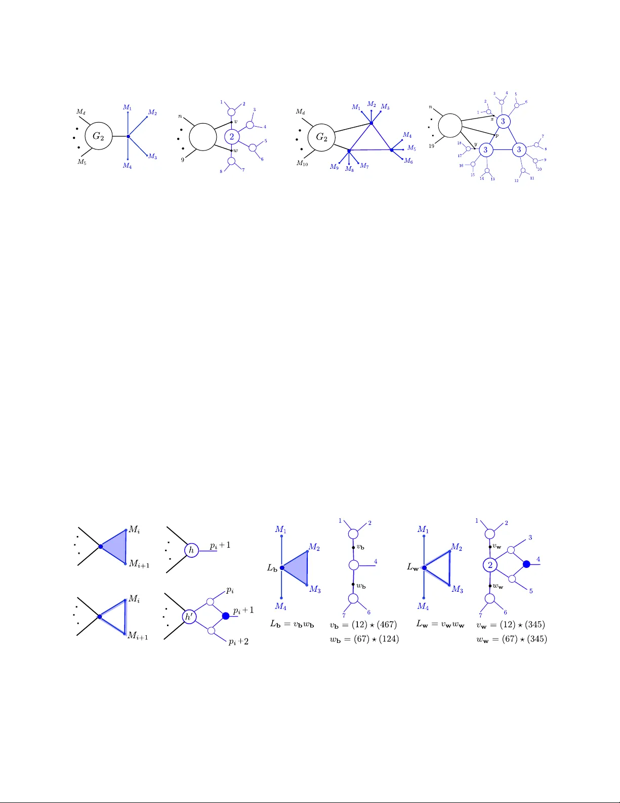
Landau Analysis in the Grassmannian Benjamin Hollering, Elia Mazzucc helli, Matteo P arisi, and Bernd Sturmfels Abstract Momen tum t wistors for scattering amplitudes in particle physics are lines in three- space. W e dev elop Landau analysis for F eynman in tegrals in this setting. The resulting discriminan ts and resultan ts are iden tiﬁed with Hurwitz and Chow forms of incidence v arieties in pro ducts of Grassmannians. W e study their degrees and factorizations, and the kinematic regimes in whic h the ﬁb ers of the Landau map are rational or real. Iden tifying this map with the amplituhedron map on p ositroid v arieties, and the asso ciated recursions with promotion maps, yields a geometric mechanism for the emergence of p ositivit y and cluster structures in planar N = 4 sup er Y ang–Mills theory . MPP-2026-49 1 In tro duction In p erturbativ e quantum ﬁeld theory , the computation of scattering amplitudes requires the ev aluation of F eynman integrals. After integration, the resulting amplitude is a meromorphic, m ultiv alued function of the external kinematic data. In general, the class of functions that can arise is not known a priori : amplitudes may in volv e m ultiple p olylogarithms, elliptic in tegrals, Calabi-Y au p eriods, etc. Ev en in the absence of a complete classiﬁcation of the relev an t function space, one ma y still ask a fundamen tal structural question: where are the singularities of the amplitude, such as p oles and branc h cuts, lo cated in kinematic space? A t the lev el of the in tegrand, the situation is considerably diﬀerent. Before integration, one has a rational function of the external and lo op kinematics. Its singularities are p oles. L andau analysis pro vides a systematic framew ork, ro oted in algebraic geometry , for studying these p oles and how they give rise to singularities of the integrated amplitude, thereb y creating a bridge betw een integrands and integrals [ 37 ]. The outcome is a collection of discriminan ts in kinematic space containing the singularities of the corresp onding in tegral. The explicit form of F eynman in tegrals dep ends on the choice of kinematic v ariables [ 49 ]. Recen t w ork of F ev ola, Mizera and T elen [ 23 , 40 ] dev elops algebraic geometry for Landau analysis in the framework of Gel’fand, Kapranov and Zelevinsky [ 27 ]. They use the Lee- P omeransky represen tation of F eynman integrals [ 49 ]. There, the integrand is go verned b y the graph p olynomial U + F . Its co eﬃcien ts are linear functions in the kinematic parameters. One seeks sp ecial parameter v alues for which the hypersurface {U + F = 0 } is singular. The 1 principal Landau determinan t in [ 23 ] is a v ariant of the principal A -determinant in [ 27 ]. It factors into irreducible discriminants whic h identify the leading singularities of the integral. Our approach rests on the momentum represen tation of F eynman in tegrals, form ulated with momen tum twistors [ 35 ] and the Grassmannian Gr(2 , 4). This formalism provides a natural compactiﬁcation of spacetime, in which c onformal symmetries of complexiﬁed Mink o wski spacetime are realized by the linear action of SL(4 , C ) [ 19 , 39 ]. W riting N and D as p olynomials in the Pl ¨ uc k er co ordinates of d + ℓ lines in P 3 , our in tegrals take the form I ( M ) = Z Γ N ( L ; M ) D ( L ; M ) d µ ( L ) . (1) The F eynman in tegral ( 1 ) is a function of the d external lines M = ( M 1 , . . . , M d ) ∈ Gr(2 , 4) d . One integrates o v er ℓ internal lines L = ( L 1 , . . . , L ℓ ) ∈ Gr(2 , 4) ℓ , for some cycle Γ and measure d µ on Gr(2 , 4) ℓ . The denominator D is a pro duct ov er pairwise line incidences, corresp onding to propagator conditions of F eynman integrals, written as in [ 36 , Eq. (2)]: D ( L ; M ) := Y a 0 . This implies p ositivit y of LS discriminants and supp orts the exp ectation that amplitudes in planar N = 4 SYM are regular on M > 0 ; • r ationality : sp ecial ﬁbers whose p oin ts are rational functions of the external kinematics M . The sp ecialized LS discriminan ts and SLS resultants factor into cluster v ariables for a higher Grassmannian. This persp ective sheds ligh t on the emergence of cluster structures in scattering amplitudes in planar N = 4 SYM. Pr op erty of the ﬁb er Ge ometric/physic al interpr etation Generic size LS degree Change of size LS discriminant and SLS resultant Realit y of p oin ts P ositivit y , regularit y on M > 0 Rationalit y of p oin ts Cluster structure 2 Momen tum twistor v ariables are well-suited for planar dual conformal inv ariant in te- grals [ 19 ]. Our results therefore ha v e direct applications to scattering amplitudes in planar N = 4 sup er Y ang–Mills (SYM) theory , where additional remark able structures arise, no- tably p ositive ge ometries and cluster algebr as [ 6 , 28 ]. A t ﬁxed multiplicit y and lo op order, the full color-ordered amplitude can b e written as a single integral of the form ( 1 ), whose in tegrand is the c anonic al form of the lo op amplituhedron [ 6 ]. The on-shell v arieties con- sidered in this work arise naturally in the b oundary stratiﬁcation of lo op amplituhedra. This p ersp ectiv e also suggests reﬁnements of Landau analysis in volving the amplituhedron b oundary and its adjoint h yp ersurface, which enco des the numerator N in ( 1 ) [ 13 , 15 , 46 ]. Related geometric approac hes in momentum-t wistors include the work of Song He et al. [ 33 ]. Another remark able structure of planar N = 4 SYM is the app earance of cluster algebras in the singularities of amplitudes, ﬁrst observ ed b y Golden et al. [ 28 ]. This was follo w ed b y the discov ery of cluster adjac encies [ 17 ] and related structures [ 31 ], culminating in the cluster b ootstrap program [ 11 ]. The recent w ork [ 21 ] explains the emergence of cluster structures at tree lev el in terms of the p ositiv e geometry of the amplituhedron. The k ey idea is to form ulate BCFW recursion in terms of maps b etw een cluster algebras, the BCFW pr omotion maps . These cluster structures are closely tied to striking p ositivit y phenomena in planar N = 4 SYM. A central exp ectation is that singularities of amplitudes do not in tersect p ositive kinematic sp ac e M > 0 , namely the quotient of a p ositive Grassmannian b y the torus action. Amplitudes are regular on M > 0 . F rom this p ersp ectiv e, Landau analysis provides a natural arena in which to study b oth p ositivit y and the cluster structure of amplitude singularities. What has remained missing in the literature is a ﬁrst-principles explanation for the emer- gence of p ositivit y and cluster structures in planar N = 4 SYM, together with a systematic algebraic-geometric framew ork for Landau analysis in momentum-t wistor space. W e provide suc h a framew ork by treating the ﬁb ers of the Landau map as primary ob jects and studying their size, degeneration, realit y , and rationalit y . The main question we address is how these ﬁb ers can b e studied intrinsically in terms of line-incidence geometry on Gr(2 , 4), and how their geometry con trols (leading, sup er-leading, and next-to-leading) Landau singularities. Our answ er combines algebraic geometry , combinatorics, and computation: we in terpret LS discriminan ts and SLS resultan ts as m ultigraded Hurwitz forms and Cho w forms, dev elop recursiv e factorization form ulas for them, and relate their positive and rational regimes to p ositroid geometry , promotion maps, and amplituhedra. This yields a mec hanism for the emergence of positivity and cluster algebraic structures in scattering amplitudes of planar N = 4 SYM, while providing eﬀectiv e to ols for computing Landau singularities. W e now discuss the structure and main contributions of this pap er. In Section 2 we re- view the representation in ( 1 ) from F eynman integrals in momen tum space. This translation arises b ecause (complexiﬁed) Mink o wski space is naturally compactiﬁed b y the Grassman- nian Gr(2 , 4). This explains why lines in P 3 and their incidences make up the denominator ( 2 ) of the integrand, and serves as the foundation for our approach to Landau analysis. Section 3 starts with a review, based on [ 36 ], of the incidence v ariety V G of a F eynman graph G . This leads us to the Landau map ψ u in ( 9 ). The ﬁbers of ψ u are the main ob jects of study in this article. W e fo cus on planar Landau diagrams arising from outerplanar graphs G . In our language G is the subgraph of the dual to a Landau diagram, whose vertices corresp ond to loop v ariables. Theorem 3.2 c haracterizes the irreducible decomp osition of 3 their incidence v arieties. In Section 4 we in tro duce discriminants for leading singularities (LS) and resultan ts for sup er-leading singularities (SLS). W e deﬁne these as m ultigraded Cho w forms [ 42 ] and Hurwitz forms [ 44 ] of line incidence v arieties. This ensures that they are irreducible. W e deriv e explicit form ulas for small graphs in Proposition 4.2 and Theorem 4.4 . In Section 5 w e determine the degree of the SLS resultan t (Theorem 5.1 ) and the exp ected degree of the LS discriminan t (Prop osition 5.3 ). Example 5.4 shows how these degrees are found with the soft w are from [ 44 , Section 6]. Section 6 is concerned with next-to-leading singularities (NLS). Here the general ﬁb er of the Landau map ψ u is a curve. The double b o x diagram yields an elliptic curve (see Theorem 6.3 ). The ﬁb er b ecomes a singular curve when the NLS discriminan t v anishes. Higher genus cases are featured in Examples 6.2 and 6.5 . The classical Poisson form ula [ 27 , § 13.1.A] computes the resultant of sev eral p olynomials b y ev aluating one p olynomial at the common zeros of the others. This leads to recursiv e form ulas for resultants. In Section 7 w e dev elop an analogous theory for LS discriminan ts and SLS resultan ts. The main results in that section are the factorization formulas in Theorems 7.4 and 7.8 . In [ 12 ] the authors explored recursive structures in Landau analysis relying on the optical theorem for scattering amplitudes. By contrast, our approach is ro oted in algebraic geometry , and it arises naturally in the language of discriminants and resultants [ 27 ]. In Section 8 w e assume that the b oundary lines in M satisfy certain prescrib ed incidences. Ph ysically , when tw o external lines intersect, the corresp onding external momen tum at that v ertex of the dual graph is on shell; otherwise it is oﬀ shell, while the propagators remain massless. This degenerations allow for geometric constructions for all p oin ts in the ﬁb er of the Landau map. These constructions translate in to rational form ulas, like those in Example 8.4 . Theorems 8.6 and 8.8 describ e this scenario for trees and triangulated ℓ -gons. Rational ﬁb ers yield factorizations of the LS discriminant, as shown in Theorem 8.11 . Section 9 centers around the Realit y Conjecture 9.1 , whic h states that the ﬁb er of the Landau map is fully real whenever the b oundary data M come from the p ositiv e Grassman- nian. Aﬃrmative results for special cases app ear in Proposition 9.2 and Theorem 9.6 . W e also presen t computational v alidations of our conjecture using tools from n umerical algebraic geometry [ 8 ]. These imply that the LS discriminant is Grassmann cop ositive (Theorem 9.6 ). P ositroids and amplituhedra hav e b ecome imp ortan t for particle ph ysics in recent years. W e connect these with line incidence v arieties in Section 10 . Our Landau map ψ u equals the amplituhedron map on a p ositroid v ariety . This rests on plabic graphs, Grassmann graphs and v ector-relation conﬁgurations [ 20 , 22 ]. Theorems 10.1 and 10.6 iden tify LS discriminants and SLS resultan ts with Chow-Lam forms and Hurwitz-Lam forms [ 45 ]. In Section 11 we show that the promotion maps in tro duced in [ 22 ] matc h our recursiv e line constructions, in whic h solutions to Sch ub ert problems are substituted in to discrimi- nan ts for smaller graphs. This pro vides the geometric mechanism underlying the recursive factorization of Landau singularities and connects rational Landau diagrams with rational p ositroids. Section 12 is devoted to the Cluster F actorization Conjecture 12.7 , which states that the irreducible factors of rational LS discriminants are cluster v ariables. This explains the emergence of cluster structures in Landau singularities from ﬁrst principles. There w e pro v e this conjecture for trees in Theorem 12.6 and present further examples b ey ond the tree case. In Section 13 we conclude with a discussion of directions for future research. 4 2 F rom F eynman Graphs to Lines in 3-Space Lines and the co ordinates that represent them corresp ond to momentum twistors in physics. The denominator D ( L ; M ) seen in ( 2 ) is a function of ℓ + d momentum twistors L i and M j . This function is a pro duct of pr op agators . The resulting p olynomial is a pairwise pro duct of momen tum twistors. A factor v anishes if and only if the tw o lines of a pair in tersect in P 3 . In what follo ws w e deriv e this represen tation ( 1 ) for a F eynman in tegral, and we explain where the lines in P 3 come from. This section is exp ository , and it is intended primarily for mathematicians to whom the many diﬀeren t lives of a F eynman integral are unfamiliar. Our p oin t of departure is the momen tum representation [ 49 , Section 2.5.1]. In what follo ws, w e assume that the given F eynman graph is planar and that spacetime is four-dimensional. W e start with d external momenta p 1 , . . . , p d and ℓ in ternal momenta k 1 , . . . , k ℓ . Each of these is a v ector in Minko wski space R 1 , 3 . In co ordinates, we write p i = ( p i 0 , p i 1 , p i 2 , p i 3 ) for i ∈ [ d ] and k j = ( k j 0 , k j 1 , k j 2 , k j 3 ) and j ∈ [ ℓ ]. Here we abbreviate [ ℓ ] = { 1 , . . . , ℓ } . Momen tum v ectors are multiplied using the Loren tzian inner pro duct on R 1 , 3 . F or example, p i · k j = p i 0 k j 0 − p i 1 k j 1 − p i 2 k j 2 − p i 3 k j 3 and k 2 j = k j · k j = k 2 j 0 − k 2 j 1 − k 2 j 2 − k 2 j 3 . (3) W e draw the giv en F eynman graph as a planar diagram. The diagram has ℓ lo ops and d legs (p endant edges). Let e b e the n um b er of in ternal edges. There are e + 1 − ℓ in ternal v ertices. W e direct the d + e edges arbitrarily . Each directed edge is lab eled by a momentum v ector as follows. The d legs are lab eled b y p 1 , . . . , p d . F or eac h lo op we select one of its edges, and w e lab el these edges b y k 1 , . . . , k ℓ . The other e − ℓ in ternal edges are lab eled so that momen tum conv ersation holds at every in ternal vertex. This means that the sum of the lab els of the incoming edges equals the sum of the lab els of the outgoing edges. With this rule, every edge has a unique lab el, which is an integer linear combination of the p i and k j . k 1 − k 3 + p 8 + p 9 + p 1 k 2 − k 1 + p 2 + p 3 + p 4 k 3 − k 2 + p 5 + p 6 + p 7 k 1 + p 1 k 2 − p 5 k 1 k 2 k 1 − p 2 k 2 + p 4 k 3 + p 7 k 3 − p 8 k 3 p 2 p 4 p 1 p 8 p 7 p 3 p 6 p 9 p 5 Figure 1: The triple p en tagon is a F eynman graph at ℓ = 3 lo ops for d = 9 in teracting particles. 5 W e write P = ( p 1 , . . . , p d ) ∈ ( R 1 , 3 ) d for the external momen ta and K = ( k 1 , . . . , k ℓ ) ∈ ( R 1 , 3 ) ℓ for the lo op momen ta. With this abbreviation, our F eynman integral takes the form I ( P ) = Z Γ N ( K ; P ) D ( K ; P ) d µ ( K ) , (4) for some cycle Γ and some integration measure d µ on ( C 1 , 3 ) ℓ . Here N , D are p olynomials in the coordinates of the momenta. The denominator D ( K ; P ) is the pro duct of the squares of all d + ℓ edge lab els. F or the legs we multiply the squares p 2 i = p 2 i 0 − p 2 i 1 − p 2 i 2 − p 2 i 3 . The in ternal edges con tribute the squares of certain linear com binations of the p i and k j . The in ternal momenta are integrated out in ( 4 ) and the resulting integral I ( P ) is a function of the external momenta. This function is transcenden tal, and one is interested in its analytic prop erties. Of sp ecial interest are the singularities, namely p oles and branch cuts. Landau analysis largely disregards the numerator, and, for our purp oses, w e ma y set N ( K ; P ) = 1. W e illustrate the labeling and the construction of the in tegral for a F eynman graph called the triple p entagon . Here ℓ = 3 , d = 9 and e = 12, so the graph has ten in ternal v ertices. One central triv alent v ertex is surrounded by a ring of nine vertices, each of which has a leg. The central vertex lies on three p en tagons. In the i th p en tagonal lo op, we use the lab el k i for the edge opp osite to the central v ertex. The lab eled triple p en tagon is shown in Figure 1 . In Figure 1 we see that, at each of the ten vertices, the sum of the incoming lab els equals the sum of the outgoing lab els. At the central vertex this is due to momen tum conv ersation: p 1 + p 2 + p 3 + p 4 + p 5 + p 6 + p 7 + p 8 + p 9 = 0 in R 1 , 3 . W e now p erform a linear change of co ordinates. Namely we replace each of the momenta b y dual v ariables. This means that w e introduce momen tum v ectors for eac h of the regions in the F eynman graph. The nine external regions are lab eled by x 1 , x 2 , . . . , x 9 . The three p en tagons are lab eled by y 1 , y 2 , y 3 , as sho wn in Figure 2 . The rule is that the v ariable labeling a directed edge is the diﬀerence of the v ariables of the regions it separates. In our example, k 1 = x 2 − y 1 , k 2 = x 5 − y 2 , k 3 = x 8 − y 3 , p 1 = x 1 − x 2 , p 2 = x 2 − x 3 , p 3 = x 3 − x 4 , . . . , p 9 = x 9 − x 1 . The co ordinates ( X , Y ) are called dual variables , b ecause they reﬂect the duality of planar graphs. Note that in general the num b er of particles of a F eynman graph need not b e the same as the num b er of external regions d . In dual v ariables, D ( K ; P ) in ( 4 ) b ecomes D ( X ; Y ) = ( x 1 − y 1 ) 2 ( x 2 − y 1 ) 2 ( x 3 − y 1 ) 2 ( x 4 − y 2 ) 2 ( x 5 − y 2 ) 2 ( x 6 − y 2 ) 2 ( x 7 − y 3 ) 2 ( x 8 − y 3 ) 2 ( x 9 − y 3 ) 2 ( y 1 − y 2 ) 2 ( y 2 − y 3 ) 2 ( y 3 − y 1 ) 2 . As b efore, each of the 12 factors in this pro duct is ev aluated using the Loren tzian inner pro duct ( 3 ). F or instance, the third factor is written in scalar quantities as follows: ( x 3 − y 1 ) 2 = ( x 30 − y 10 ) 2 − ( x 31 − y 11 ) 2 − ( x 32 − y 12 ) 2 − ( x 33 − y 13 ) 2 . (5) W e ﬁnally p erform a second linear change of co ordinates, namely from the dual v ariables ( X , Y ) to momentum t wistors ( L , M ) = ( L 1 , . . . , L ℓ , M 1 , . . . , M d ). Each L j and each M k is a line in P 3 . The ℓ + d lines can b e represented as the ro w spans of 2 × 4 matrices as follo ws: L j =  1 0 y j 0 + y j 3 y 1 j − iy 2 j 0 1 y j 1 + iy j 2 y j 0 − y j 3  and M k =  1 0 x k 0 + x k 3 x k 1 − ix k 2 0 1 x k 1 + ix k 2 x k 0 − x k 3  . (6) 6 y 1 y 2 y 3 x 1 x 6 x 2 x 5 x 3 x 4 x 7 x 9 x 8 L 1 L 2 L 3 M 3 M 1 M 2 M 4 M 6 M 5 M 7 M 8 M 9 Figure 2: Regions of the triple p en tagon lab eled b y dual v ariables (left). The dual graph lab eled b y momentum twistors (righ t). These are lines in 3-space with prescribed incidences. Here, i = √ − 1. The formula ( 6 ) is derived in [ 36 , Section 8]. Its key prop ert y is as follows: the determinant of an y 4 × 4 matrix obtained by stacking tw o of the 2 × 4 matrices v anishes if and only if the t wo lines in tersect in P 3 . Remark ably , the factors in the denominator of our integrand are precisely the algebraic translations of this geometric condition. This is the con ten t of [ 36 , Equation (29)]. F or instance, the expression in ( 5 ) is the 4 × 4 determinant ⟨ L 1 M 3 ⟩ := det  L 1 M 3  = ( x 30 − y 10 ) 2 − ( x 31 − y 11 ) 2 − ( x 32 − y 12 ) 2 − ( x 33 − y 13 ) 2 . W e use the notation ⟨ L j L k ⟩ and ⟨ L j M k ⟩ for such 4 × 4 determinants. Eac h of these deter- minan ts is the inner pro duct of tw o Pl ¨ uck er co ordinate vectors, as in [ 36 , Equation (2)]. In summary , for the triple p en tagon, the denominator D ( L ; M ) in ( 2 ) is the pro duct ⟨ L 1 M 1 ⟩⟨ L 1 M 2 ⟩⟨ L 1 M 3 ⟩⟨ L 2 M 4 ⟩⟨ L 2 M 5 ⟩⟨ L 2 M 6 ⟩⟨ L 3 M 7 ⟩⟨ L 3 M 8 ⟩⟨ L 3 M 9 ⟩⟨ L 1 L 2 ⟩⟨ L 1 L 3 ⟩⟨ L 2 L 3 ⟩ . (7) The 12 factors corresp ond to the 12 edges in the dual graph on the right in Figure 2 . The denominator is D ( X ; Y ) in dual v ariables, and it equals D ( K ; P ) in ( 4 ) when written in the original momen tum co ordinates. The latter is the pro duct of the 12 edge lab els in Figure 1 . The same t w o co ordinate transformations can b e carried out for any planar F eynman graph. One ends up with a graph with ℓ vertices L i and d vertices M k , lik e that shown on the right of Figure 2 . The latter graph sp eciﬁes incidence relations among ℓ + d lines in P 3 . T o study singularities of the in tegral ( 1 ), one in tro duces L andau diagr ams . A Landau diagram lo oks lik e a scalar F eynman graph, and it represents a stratum in the v anishing lo cus of ( 2 ). The left picture in Figure 2 is a Landau diagram for the underlying F eynman in tegral, where all propagators in ( 7 ) are set to zero. In the follo wing, we rather work with the dual graph to a Landau diagram, as for example the graph on the right in Figure 2 . F or simplicit y , we also refer to the dual graph as the Landau diagram. That diagram precisely enco des the incidences of lines in 3-space cutting out the stratum under consideration. 7 3 Incidence V arieties and the Landau Map W e now turn to incidence v arieties of lines in P 3 , follo wing the set-up in [ 36 , Section 3]. Our am bient space Gr(2 , 4) ℓ is the pro duct of ℓ Grassmannians which sits inside ( P 5 ) ℓ via the Pl ¨ uck er em b edding. F or a graph G ⊂  [ ℓ ] 2  , the incidence v ariet y V G is the set of tuples ( L 1 , . . . , L ℓ ) such that ⟨ L i L j ⟩ = 0 for all ij ∈ G . The dimension of V G and a characterization for which graphs V G is irreducible or a complete in tersection is given in [ 36 , Section 5]. The multide gr e e [ V G ] is the class of the incidence v ariety V G in the Cho w ring A ∗  ( P 5 ) ℓ , Z  = Z [ t 1 , t 2 , . . . , t ℓ ] / ⟨ t 6 1 , t 6 2 , . . . , t 6 ℓ ⟩ . W e write this as a homogeneous p olynomial whose degree is the co dimension of V G in ( P 5 ) ℓ : [ V G ] = X u ∈ N ℓ γ u · t 5 − u 1 1 t 5 − u 2 2 · · · t 5 − u ℓ ℓ . (8) Here u runs ov er nonnegative in teger v ectors u with | u | = P ℓ i =1 u i = dim( V G ) =: d . The co eﬃcien t γ u is the LS de gr e e of the auxiliary graph G u , whic h is obtained by attaching u i p endan t edges at the v ertex i of G . Hence G u has ℓ + d vertices and | G | + d edges. In relation to Section 2 , the auxiliary graph G u should b e understo od as the planar dual of a le ading L andau diagr am . Geometrically , the LS degree γ u is the degree of the L andau map ψ u : Gr(2 , 4) ℓ + r → Gr(2 , 4) d , ( L , M ) → M . (9) This map deletes the ℓ internal lines. The ﬁb er of ψ u o v er a p oin t M = ( M 1 , . . . , M d ) ∈ Gr(2 , 4) d consists of all line conﬁgurations L = ( L 1 , . . . , L ℓ ) which satisfy d Sch ub ert condi- tions. Namely , the i th line L i is required to satisfy ⟨ L i M j ⟩ = 0 for the u i external lines M j where j is inciden t to i in G u . Hence, γ u coun ts the exp ected n umber of leading singularities. Example 3.1 (T riangle) . Let ℓ = 3 and G = { 12 , 13 , 23 } . The v ariety V G is the union of t w o irreducible comp onen ts V [3] and V ∗ [3] of dimension d = 9 in Gr(2 , 4) 3 . Conﬁgurations in V [3] are triples of concurren t lines, while conﬁgurations in V ∗ [3] are triples of coplanar lines. W e ha ve [ V G ] = [ V [3] ] + [ V ∗ [3] ], and the t wo irreducible components ha v e the same multidegree: [ V [3] ] = [ V ∗ [3] ] = 4 t 1 t 2 t 3 ( t 1 + t 2 )( t 1 + t 3 )( t 2 + t 3 ) = 4  X π ∈ S 3 t 3 π (1) t 2 π (2) t π (3)  + 8 t 2 1 t 2 2 t 2 3 . W e no w ﬁx u = (3 , 3 , 3). The graph G u is sho wn on the right in Figure 2 . The LS degree γ u equals 16 = 8 + 8. Indeed, given 9 general lines M = ( M 1 , . . . , M 9 ) in P 3 , there are precisely 8 concurrent triples L = ( L 1 , L 2 , L 3 ) which satisfy the 9 Sch ub ert conditions they imp ose: ⟨ L 1 M 1 ⟩ = ⟨ L 1 M 2 ⟩ = ⟨ L 1 M 3 ⟩ = ⟨ L 2 M 4 ⟩ = ⟨ L 2 M 5 ⟩ = ⟨ L 2 M 6 ⟩ = ⟨ L 3 M 7 ⟩ = ⟨ L 3 M 8 ⟩ = ⟨ L 3 M 9 ⟩ = 0 . Similarly , there are 8 coplanar triples L satisfying these equations. These L form a Cayley o ctad , i.e. they are found by in tersecting three quadratic surfaces in P 3 . See [ 36 , Example 3.2]. 8 The physical meaning of the Landau map ψ u concerns the singularities of the F eynman in tegral ( 4 ). In Section 2 we show ed that this integral can b e written in the form ( 1 ), where we are integrating ov er L in Gr(2 , 4) ℓ and the resulting function of M has its domain in Gr(2 , 4) d . The denominator D ( L ; M ) is the pro duct of propagators, and these form an arrangemen t of h yp ersurfaces. Higher-co dimension singular lo ci are obtained by intersecting subsets of these hypersurfaces, that is, by setting a subset of propagators to zero, D i 1 = · · · = D i k = 0. Singularities of maximal co dimension are called le ading singularities (LS). These are the p oin ts in the ﬁb ers of ψ u . Their num b er is the LS degree γ u , which w e read oﬀ from [ V G ]. An imp ortan t ingredien t in our framew ork is the decomp osition of the v ariet y V G in to irreducible comp onen ts. W e denote these irreducible v arieties by V G,σ where σ runs ov er an appropriate ﬁnite set of lab els. F or man y graphs of interest, these lab els arise from concurren t and coplanar triples, as seen in Example 3.1 . W e will no w mak e this precise. In graph theory , a graph G on [ ℓ ] is called outerplanar if it is a subgraph of a triangulated ℓ -gon. The v ertices are lab eled in cyclic order 1 , 2 , . . . , ℓ . Being outerplanar is a strong form of planarity . Similar to Kuratowski’s c haracterization of planar graphs by excluded minors, a graph G is outerplanar if and only if it has no subgraph that is a sub division of K 4 or K 2 , 3 . If G is outerplanar then its triangles are visible in the planar drawing. W e write τ ( G ) for the n umber of triangles. F or instance, if G is a triangulated ℓ -gon then τ ( G ) = ℓ − 2 and the v ariety V G has 2 ℓ − 2 irreducible comp onen ts [ 36 , Theorem 4.10]. These comp onen ts are lab eled by the bicolorings σ of the triangles. A black triangle means that three lines are concurren t, while a white triangle means that they are coplanar. See [ 36 , Figure 1] for ℓ = 4. Theorem 3.2. L et G b e an outerplanar gr aph. Then the incidenc e variety V G is a c omplete interse ction. It has pr e cisely 2 τ ( G ) irr e ducible c omp onents, as describ e d ab ove, one for e ach bic oloring σ of the triangles. In p articular, V G is irr e ducible when the gr aph G is triangle-fr e e. Pr o of. Every outerplanar graph G is (2 , 3)-sparse, i.e. it is independent in the rigidit y matroid [ 36 , Remark 4.4]. W e claim that G is strictly con traction stable. This notion was deﬁned in [ 36 , Section 5]. W e then conclude, b y [ 36 , Theorem 5.4], that V G is a complete intersection. Our claim states that, for an y partition J = { J 1 , . . . , J r } of [ ℓ ] with singletons omitted: | G J | + 4( | J 1 | + | J 2 | + · · · + | J r | − r ) > | G | . In this formula, G J is the graph on ℓ − s J v ertices obtained by iden tifying all vertices in eac h J i , merging parallel edges, and deleting resulting lo ops. Here s J = | J 1 | + · · · | J r | − r . Note that the graph ( G { J 1 } ) { J 2 } obtained by ﬁrst con tracting with resp ect to the partition { J 1 } and then { J 2 } is the same as that obtained by con tracting with resp ect to { J 1 , J 2 } . Therefore, it suﬃces to prov e the inequalit y for partitions with only one blo c k. Let J = { J 1 } b e a partition of [ ℓ ] with one non-singleton blo c k. W e m ust sho w that | G | − | G J | < 4 | J 1 | − 4. Let J c 1 = [ ℓ ] \ [ J 1 ], and H = { ij ∈ G | i ∈ J 1 , j ∈ J c 1 } , and K = { i ∈ J c 1 | ij ∈ G for some j ∈ J 1 } . The num b ers of edges in our graphs are | G | = | G [ J 1 ] | + | G [ J c 1 ] | + | H | and | G J | = | G [ J c 1 ] | + | K | , where G [ S ] is the subgraph of G induced on S . Hence, | G | − | G J | = | G [ J 1 ] | + | H | − | K | . Since G is (2,3)-sparse, | G [ J 1 ] | ≤ 2 | J 1 | − 3, so it remains to show that | H | − | K | < 2 | J 1 | − 1. 9 Note that H is bipartite with parts J 1 and K . As a minor of G , it is outerplanar. It is easy to show, b y induction, that | H | ≤ 2 | J 1 | + | K | − 2 for an y outerplanar bipartite graph H . W e next pro v e that V G has 2 τ ( G ) irreducible comp onen ts indexed by bicolorings of G ’s triangles. F or ℓ ≤ 3 this is clear. Let ℓ > 3. Since G is outerplanar, there exists a vertex v of degree r ≤ 2. Consider the map π : Gr(2 , 4) ℓ → Gr(2 , 4) ℓ − 1 whic h forgets the line asso ciated to v . The image of π is V e G , where e G is the graph on ℓ − 1 vertices obtained from G by deleting v . By our induction hypothesis, V e G = X e G has 2 τ ( e G ) irreducible comp onen ts. Let V ˜ σ ⊂ V e G b e an y irreducible comp onent, giv en by a bicoloring ˜ σ of the τ ( e G ) triangles in e G . Supp ose that r = 1. The ﬁb er is irreducible and π deﬁnes a ﬁb er bundle ov er V ˜ σ . Hence there exists an irreducible comp onen t V σ ⊂ V G asso ciated to V ˜ σ . In this case, τ ( G ) = τ ( e G ) and thus V G has 2 τ ( G ) irreducible comp onen ts indexed by the bicolorings of triangles of G . No w supp ose that r = 2 and denote b y u and w the vertices adjacen t to v . If uw / ∈ G , then π − 1 ( V ˜ σ ) is again irreducible and the desired result follows as in the r = 1 case. Lastly , if r = 2 and uw ∈ G , τ ( G ) = τ ( ˜ G ) + 1 and the ﬁb er π − 1 ( V ˜ σ ) = V σ w ∪ V σ b is the union of t w o irreducible v arieties corresp onding to the bicolorings of the new triangle { u, v , w } in G . The concurren t comp onen t V σ b can b e parametrized by taking the line corresp onding to v to b e spanned by the intersection p oin t of L u and L w and a new generic p oin t in P 3 . The coplanar comp onen t V σ w can b e parametrized similarly . This parametrization yields a Zariski-open subset of V σ b where L u  = L w , how ever since V G is strictly contraction-stable, the subv ariety X G where all ℓ lines are distinct is equal to V G . Th us we see that π − 1 ( V ˜ G ) = V G = X G has 2 τ ( G ) irreducible comp onen ts indexed b y the bicolorings of the triangles of G as required. A planar graph can hav e more or few er irreducible comp onen ts than 2 τ ( G ) , where τ ( G ) is the n umber its triangles in a planar drawing. Example 3.3. A ﬁrst example is the kite graph G = { 12 , 13 , 14 , 23 , 34 , 25 , 45 } . The v ariet y V G is a complete intersection of co dimension 7, but it has six irreducible components, whereas G has only tw o triangles: 6 > 2 τ ( G ) = 4. Note that G is a subgraph of the wheel W 5 . Understanding the irreducible decomposition for planar graphs b eyond the outerplanar case remains an interesting op en problem. A ﬁrst family for which such a decomp osition is kno wn is giv en b y the wheel graphs G = W ℓ : by [ 36 , Theorem 4.9], the n um b er of irreducible comp onen ts is 2 τ ( G ) − 2 τ ( G ), which is smaller than the exp ected count 2 τ ( G ) . 4 Discriminan ts and Resultan ts Fix a graph G on [ ℓ ], and let d b e the dimension of its incidence v ariet y V G . Consider u ∈ N ℓ suc h that | u | = d and γ u ≥ 2. F or generic external data M ∈ Gr(2 , 4) d , the ﬁb er ψ − 1 u ( M ) con tains precisely γ u line conﬁgurations L . W e are interested in the condition on M suc h that tw o p oin ts in ψ − 1 u ( M ) come together. This condition gives a hypersurface in Gr(2 , 4) d , deﬁned by a unique (up to scaling) p olynomial ∆ G,u ( M ), whic h we call the LS discriminant . First supp ose that V G is irreducible. In this case, ∆ G,u ( M ) is an irreducible p olynomial. Namely , it is precisely the multigr ade d Hurwitz form of V G . This is deﬁned in [ 44 ] and it represen ts a h yp ersurface in ( P 5 ) d . This hypersurface lives in Gr( u 1 , 6) × · · · × Gr( u d , 6), 10 and w e write it in primal Stiefel co ordinates. This means that M is represented b y a 6 × d matrix whose columns are Pl ¨ uck er co ordinates on the d factors of ( P 5 ) d . F urthermore, in our application to Landau analysis, w e alw a ys restrict ∆ G,u ( M ) to Gr(2 , 4) d . This means that eac h column of the 6 × d matrix represen ting M satisﬁes the quadratic Pl ¨ uck er relation. Example 4.1 ( ℓ = 1) . W e hav e u = (4), as in [ 36 , Example 3.1], and ψ − 1 u ( M ) consists of the t w o lines that are incident to four lines M 1 , M 2 , M 3 , M 4 . Here the LS discriminan t equals ∆ K 1 , (4) = det    0 M 1 M 2 M 1 M 3 M 1 M 4 M 1 M 2 0 M 2 M 3 M 2 M 4 M 1 M 3 M 2 M 3 0 M 3 M 4 M 1 M 4 M 2 M 4 M 3 M 4 0    , where M i M j := ⟨ M i M j ⟩ . (10) This Gram determinan t v anishes when the tw o lines coincide. See [ 44 , Example 6.1]. W e next analyze the graph G = { 12 } with ℓ = 2 v ertices. Set u = (4 , 3). F or simplicit y of notation we write L = ( X , Y ) and M = ( A, B , C , D ; E , F , G ). The v ariety V G is the h yp ersurface in Gr(2 , 4) 2 deﬁned by X Y = 0. The equations for our Sch ub ert problem are AX = B X = C X = D X = E Y = F Y = GY = 0 . (11) These are inner pro duct lik e AX = a 12 x 34 − a 13 x 24 + a 14 x 23 + a 23 x 14 − a 24 x 13 + a 34 x 12 . The LS degree equals γ u = 4, i.e. there are four pairs L ∈ V G suc h that ( 11 ) holds. The LS discriminant ∆ G,u has degree (4 , 4 , 4 , 4 , 4 , 4 , 4) in the entries of the seven giv en Pl¨ uck er v ectors A, B , C , D , E , F , G . W e will present an explicit formula in Prop ositions 4.2 and 4.3 . Assuming that A, B , C, D , E , G span R 6 , and in tro ducing v ariables x 1 , x 2 , . . . , x 6 , we write X = x 1 A + x 2 B + x 3 C + x 4 D + x 5 E + x 6 G. This basic choice is recorded in the following Gram matrix, whic h is symmetric of size 6 × 6: G =       0 AB AC AD AE AG AB 0 B C B D B E B G AC B C 0 C D C E C G AD B D C D 0 DE DG AE B E C E D E 0 E G AG B G C G D G E G 0       . (12) Our assumption that X intersects A, B , C , D yields four linear equations in x 1 , . . . , x 6 , namely AX = AB x 2 + AC x 3 + ADx 4 + AE x 5 + AGx 6 = 0 , B X = AB x 1 + B C x 3 + B D x 4 + B E x 5 + B Gx 6 = 0 , C X = AC x 1 + B C x 2 + C D x 4 + C E x 5 + C Gx 6 = 0 , D X = AD x 1 + B D x 2 + C D x 3 + DE x 5 + DGx 6 = 0 . (13) The Pl ¨ uck er relation X X = 2( x 12 x 34 − x 13 x 24 + x 14 x 23 ) = 0 implies the quadratic constraint X X = AB x 1 x 2 + AC x 1 x 3 + ADx 1 x 4 + · · · + D E x 4 x 5 + DGx 4 x 6 + E Gx 5 x 6 = 0 . (14) F or the LS discriminant, w e require that the tw o transversal lines of E , F , G and X coincide: det    0 E F E G E X E F 0 F G F X E G F G 0 GX E X F X GX 0    = ( AE 2 F G 2 − 2 AE AF E G F G − · · · + AG 2 E F 2 ) x 2 1 + · · · = 0 . (15) 11 Prop osition 4.2. The LS discriminant e quals 1 / det( G ) 2 times the r esultant of six e quations in six unknowns, namely the four line ar forms in ( 13 ) and the two quadrics in ( 14 ) and ( 15 ). Pr o of. W e consider four linear equations Tx = 0 and tw o quadratic equations x t Ux = x t Vx = 0, where T is a 4 × 6 matrix and U and V are symmetric 6 × 6 matrices. The resultan t is a polynomial of degree 20 in the 66 = 4 · 6 + 2 ·  7 2  unkno wn en tries of these matrices. Namely , it has degree 4 in each ro w of T and it is quadratic in each of U and V . W e now substitute ( 13 ) for T , ( 14 ) for U , and ( 15 ) for V . A computation shows that the resulting p olynomial is nonzero, and it has degree 26 = 4 + 4 + 4 + 4 + 2 + 8 in the 28 quantities AB , AC , . . . , F G . More precisely , it is multihomogeneous of degree (8 , 8 , 8 , 8 , 8 , 4 , 8) in the sev en Pl¨ uck er v ectors A, B , C , D , E , F , G . The extraneous factor has degree (4 , 4 , 4 , 4 , 4 , 0 , 4). W e ﬁnd that it is the square of the determinant of the Gram matrix G . It remains to giv e a form ula for the resultan t Res 1 , 1 , 1 , 1 , 2 , 2 of six homogeneous equations in six unknowns, of the indicated degrees. Let f 1 , f 2 , f 3 , f 4 denote the linear forms in Tx , and set f 5 = xUx t and f 6 = xVx t . Our formula is an explicit p olynomial in the 66 co eﬃcien ts. F or i = 0 , 1 , . . . , 6, write σ i for the op erator which replaces the unknowns x 1 , . . . , x i with new unkno wns y 1 , . . . , y i . Let ∆ b e the 6 × 6 matrix whose entries are the divided diﬀerences ∆ ij = σ i − 1 ( f j ) − σ i ( f j ) x i − y i for 1 ≤ i, j ≤ 6 . The B´ ezoutian B is the 6 × 6-matrix whose entries are the mixed partials ∂ 2 det(∆) /∂ x i ∂ y j . These entries are multilinear forms in the co eﬃcien ts of our p olynomials f 1 , f 2 , f 3 , f 4 , f 5 , f 6 . Prop osition 4.3. The r esultant for four line ar forms and two quadrics in six unknowns is Res 1 , 1 , 1 , 1 , 2 , 2 ( T , U , V ) = det  B T t T 0  . (16) This 10 × 10 determinant is a p olynomial of de gr e e (4 , 4 , 4 , 4 , 2 , 2) in the 66 c o eﬃcients. Pr o of. This is an instance of the determinantal formulas for resultants derived by D’Andrea and Dic kenstein in [ 14 ]. The critical degree for our equations is t 6 = 1 + 1 + 1 + 1 + 2 + 2 − 6 = 2. Setting t = 1 in [ 14 , Lemma 5.3], w e obtain the blo ck matrix of size 10 × 10 sho wn in ( 16 ). F or general graphs, the v ariet y V G is reducible. In this case, ∆ G,u is a pro duct whose irreducible factors include the LS discriminan ts ∆ G,σ,u of the comp onen ts V G,σ . In addition, there are certain mixed factors. W e sho w this for the triangle graph G = K 3 with u = (3 , 3 , 3). Theorem 4.4. The LS discriminant ∆ K 3 ,u has de gr e e (48 , 48 , 48) . It has thr e e irr e ducible factors, c orr esp onding to the thr e e sc enarios for two of the 8 + 8 solutions to c ome to gether: • the LS discriminant ∆ K 3 ,u, b of the c oncurr ent c omp onent V [3] has de gr e e (16 , 16 , 16) , • the LS discriminant ∆ K 3 ,u, w of the c oplanar c omp onent V ∗ [3] has de gr e e (16 , 16 , 16) , • the squar e of the irr e ducible mixe d LS discriminant, which has de gr e e (8 , 8 , 8) . The last factor vanishes when a solution of ( 11 ) on V [3] mer ges with a solution on V ∗ [3] . 12 This theorem is prov ed by a symbolic computation with Macaulay2 [ 30 ]. In the next section we discuss an indep enden t v alidation based on the techniques in [ 44 , Section 6]. Another singular scenario for the integral ( 1 ) arises when the Sch ub ert problem is ov er- constrained, namely if u ∈ N ℓ satisﬁes | u | = d + 1. The Landau map ψ u is not surjective, but its image is a hypersurface in Gr(2 , 4) d +1 . This hypersurface is deﬁned by a p olynomial R G,u whic h we call the SLS r esultant . A sup erle ading singularity (SLS) arises when R G,u ( M ) = 0. Example 4.5 ( ℓ = 1) . The SLS resultant is the condition for the ﬁv e lines M j in P 3 to hav e a common transv ersal. This is the determinant of the Gram matrix for ﬁv e Pl ¨ uc ker vectors: R K 1 , (5) ( M ) = det      0 M 1 M 2 M 1 M 3 M 1 M 4 M 1 M 5 M 1 M 2 0 M 2 M 3 M 2 M 4 M 2 M 5 M 1 M 3 M 2 M 3 0 M 3 M 4 M 3 M 5 M 1 M 4 M 2 M 4 M 3 M 4 0 M 4 M 5 M 1 M 5 M 2 M 5 M 3 M 5 M 4 M 5 0      . (17) W e see that this SLS resultant has degree (2 , 2 , 2 , 2 , 2) as a hypersurface in ( P 5 ) 5 . Example 4.6 ( ℓ = 2) . Let G = { 12 } and u = (4 , 4). W e augment the system ( 11 ) by one more equation H Y = 0. Here, the SLS resultan t R G,u is a large irreducible p olynomial whic h is homogeneous of degree 4 in each of the eight Pl ¨ uc k er vectors in M = ( A, B , . . . , G, H ). Example 4.7 ( ℓ = 3) . Let G = K 3 as in Theorem 4.4 , but now we tak e u = (4 , 3 , 3). The SLS resultan t is the pro duct of tw o irreducible factors, one for each irreducible comp onen t of V G . Eac h of these tw o factors has degree (8 , 8 , 8 , 8; 4 , 4 , 4; 4 , 4 , 4) in the 10 external lines in M . W e conclude that the SLS resultant R K 3 ,u has degree (16 , 16 , 16 , 16; 8 , 8 , 8; 8 , 8 , 8). In the next section we shall see that these num b ers are the LS degrees γ u − e i for i = 1 , 2 , 3. 5 Cho w and Hurwitz Osserman and T rager [ 42 ] introduced the m ultigraded Chow forms for arbitrary subv arieties in a pro duct of pro jectiv e spaces. Their deﬁnition sho ws that the multigraded Chow forms of the incidence v ariety V G are precisely the SLS resultants R G,u , for the v arious vectors u ∈ N d that satisfy | u | = d + 1. These Chow forms are multiplicativ e o v er the irreducible decomp osition of V G . Hence R G,u is the pro duct of the irreducible SLS resultants R G,u,σ , where V G,σ ranges o v er the comp onen ts of V G . F or instance, if G is outerplanar then this pro duct is o ver the 2 τ ( G ) bicolorings of the triangles of G . F rom [ 42 , Theorem 1.2] we obtain: Theorem 5.1. The SLS r esultant R G,u is a homo gene ous p olynomial of de gr e e γ u − e i in the six Pl ¨ ucker c o or dinates of e ach of the u i external lines that ar e attache d to vertex i of G . It is imp ortant to recognize the diﬀeren t co ordinate systems that o ccur in this result. In the setting of [ 42 ], the m ultigraded Chow form is a hypersurface in Gr( u 1 , 6) × · · · × Gr( u d , 6), and the degree γ u − e i refers to Pl ¨ uc k er co ordinates on the i th factor Gr( u i , 6). Eac h line that is attached to the i th vertex of G has its own six Pl ¨ uc ker co ordinates, and w e write these as the rows of a u i × 6 matrix. That matrix furnishes primal Stiefel co ordinates for Gr( u i , 6) in 13 the set-up of Osserman and T rager. Since the u i × u i minors of this u i × 6 Stiefel matrix are linear in each row, the degree of R G,u in each of the u i lines in the i -th blo c k of M coincides with the degree on Gr( u i , 6) in [ 42 ]. And this is the co eﬃcien t γ u − e i in the m ultidegree [ V G ]. Examples 4.6 and 4.7 illustrate Theorem 5.1 . W e present a case study for a larger graph. Example 5.2 ( ℓ = 5) . Consider the triangulated p en tagon G = { 12 , 13 , 14 , 15 , 23 , 34 , 45 } . Its ideal I G is radical, and a complete intersection by [ 36 , Theorem 5.4]. W e also know from [ 36 , Theorem 4.10] that the ideal has the prime decomp osition I G = I 12345 ∩ I ∗ 12345 ∩ ( I 123 + I ∗ 1345 ) ∩ ( I ∗ 123 + I 1345 ) ∩ ( I 1234 + I ∗ 145 ) ∩ ( I ∗ 1234 + I 145 ) ∩ ( I 123 + I ∗ 134 + I 145 ) ∩ ( I ∗ 123 + I 134 + I ∗ 145 ) . Since I G is a complete intersection, its multidegree is the pro duct of its generating degrees: [ I G ] = 32 t 1 t 2 t 3 t 4 t 5 ( t 1 + t 2 )( t 1 + t 3 )( t 1 + t 4 )( t 1 + t 5 )( t 2 + t 3 )( t 3 + t 4 )( t 4 + t 5 ) . The expansion is a sum of 82 terms of degree 12, whose co eﬃcien ts add up to 4096. F or each of the eigh t irreducible components V G,σ w e compute the multidegree [ V G,σ ], and w e c heck that these add up correctly , i.e. [ I 12345 ] + [ I ∗ 12345 ] + · · · + [ I ∗ 123 + I 134 + I ∗ 145 ] = [ I G ]. Among the eigh t summands, there are four distinct pairs of multidegrees. Namely , we ﬁnd the follo wing: (a) [ I 12345 ] = [ I ∗ 12345 ] has 30 terms with co eﬃcien ts in { 4 , 8 } , (b) [ I 123 + I ∗ 1345 ] = [ I ∗ 123 + I 1345 ] has 56 terms with co eﬃcien ts in { 4 , 8 , 12 , 16 , 24 } , (c) [ I 1234 + I ∗ 145 ] = [ I ∗ 1234 + I 145 ] has 56 terms with co eﬃcien ts in { 4 , 8 , 12 , 16 , 24 } , (d) [ I 123 + I ∗ 134 + I 145 ] = [ I ∗ 123 + I 134 + I ∗ 145 ] has 82 terms with co eﬀs in { 4 , 8 , 12 , 16 , 20 , 24 , 32 } . Equipp ed with this data, w e can now apply Theorem 5.1 to deriv e the exp ected m ultidegrees of all irreducible SLS resultants R G,u,σ . Here σ is a bicoloring that marks one of the eight irreducible comp onen ts, and u ranges o ver all vectors in N 5 that satisfy | u | = d + 1 = 14. W e consider the ﬁv e vectors u that hav e four entries 2 and one entry 3. Each vector sp eciﬁes a graph G u with 19 vertices and 21 edges, and hence a planar Landau diagram with 19 regions. The degrees of the asso ciated SLS resultants are listed in the following table: u = (2 , 3 , 3 , 3 , 3) (3 , 2 , 3 , 3 , 3) (3 , 3 , 2 , 3 , 3) (3 , 3 , 3 , 2 , 3) (3 , 3 , 3 , 3 , 2) (a) (0 , 8 , 8 , 8 , 8) (8 , 0 , 8 , 8 , 8) (8 , 8 , 0 , 8 , 8) (8 , 8 , 8 , 0 , 8) (8 , 8 , 8 , 8 , 0) (b) (16 , 8 , 24 , 16 , 16) (8 , 0 , 8 , 8 , 8) (24 , 8 , 16 , 16 , 16) (16 , 8 , 16 , 0 , 8) (16 , 8 , 16 , 8 , 0) (c) (16 , 16 , 16 , 24 , 8) (16 , 0 , 8 , 16 , 8) (16 , 8 , 0 , 16 , 8) (24 , 16 , 16 , 16 , 8) (8 , 8 , 8 , 8 , 0) (d) (32 , 16 , 32 , 32 , 16) (16 , 0 , 8 , 16 , 8) (32 , 8 , 16 , 24 , 16) (32 , 16 , 24 , 16 , 8) (16 , 8 , 16 , 8 , 0) Observ e that the degree in the Pl ¨ uc k er co ordinates of each external line M j attac hed to the same internal line L i is the same. F or instance, the ﬁrst entry (0 , 8 , 8 , 8 , 8) in the table ab ov e reﬂects that this SLS resultan t has degree 0 in the 2 external lines attac hed to v ertex 1, and degree 8 in the external lines attac hed to all other v ertices. The last ro w (d) concerns the t wo most in teresting comp onen ts V G,σ , where σ assigns alternating colors to the three triangles in G . The SLS resultant in the middle is an irreducible p olynomial of degree (32 , 8 , 16 , 24 , 16) in M = ( M 1 , M 2 , M 3 , M 4 , M 5 ). T o obtain the degree of R G,u , we add the degrees of R G,u,σ 14 for each of the eight comp onen ts giv en b y the bicolorings σ . Since the degrees are preserved under Ho dge star duality , we add twice the four degrees in the third column. W e see that the reducible SLS resultant R G,u = Q σ R G,u,σ has degree (160 , 64 , 64 , 128 , 96) in M . Pratt, So domaco and Sturmfels [ 44 ] introduced the multigraded Hurwitz forms for an arbitrary sub v ariety in a pro duct of pro jective spaces. Their deﬁnition shows that the m ulti- graded Cho w forms of the incidence v ariety V G are precisely the LS discriminan ts ∆ G,u , for the v arious v ectors u ∈ N d that satisfy | u | = d . These Hurwitz forms are reducible when V G has m ultiple comp onen ts. But the factorization is more complicated than that for Chow forms. W e saw this in Theorem 4.4 for the incidence v ariety of the triangle, V K 3 ⊂ ( P 5 ) 3 . A complete understanding of the factorization prop erties of LS discriminants would re- quire a multigraded extension of the results in [ 48 , Section 4] on degenerations of Hurwitz forms. W e shall not pursue this here, but instead w e often work with irreducible V G or restrict to an irreducible comp onen t V G,σ . F or instance, we can take G to b e a triangle-free outerplanar graph. Ev en the sp ecial case when G is a tree is of in terest for our application. Consider the ℓ + | G | equations that deﬁne V G in ( P 5 ) ℓ . First, w e ha ve the ℓ Pl ¨ uck er relations, and these ha v e degrees 2 e i for i = 1 , . . . , ℓ . Second, w e ha ve the equations ⟨ L i L j ⟩ = 0 for all edges ij ∈ G , and these hav e degrees e i + e j . Since V G is a complete intersection, the follo wing formula holds for its multidegree from which one easily extracts the LS degrees γ u : [ V G ] = 2 ℓ · t 1 t 2 · · · t ℓ · Y ij ∈ G ( t i + t j ) . (18) In [ 44 , Section 6], the authors compare V G with the complete intersection deﬁned by generic equations of the same degrees. The following result is pro ved in [ 44 , Corollary 6.3]. Prop osition 5.3. The LS discriminant ∆ G,u is a p olynomial of de gr e e ( b 1 , . . . , b ℓ ) wher e b i ≤ 2 γ u + X j ∈ [ ℓ ] u j + δ ij > 0 γ u + e i − e j ·  1 − u j − δ ij + degree G ( i )  for al l i ∈ [ ℓ ] . (19) The righ t hand side in ( 19 ) is the exp ected degree of the LS discriminan t. Here δ ij is Kronec k er’s delta, and degree G ( i ) is the n umber of edges in G that are incident to vertex i . W e conjecture that equalit y holds in ( 19 ) if we tak e extraneous factors in to consideration. Let us explain what this conjecture means for ℓ = 2. The LS discriminant ∆ K 2 , (4 , 3) w as featured in Proposition 4.2 , where w e sa w that its degree is ( b 1 , b 2 ) = (4 , 4). The upper b ound in Proposition 5.3 equals (8 , 4). This is the true degree of the multigraded Hurwitz form for the complete in tersection of degrees (2 , 0) , (0 , 2) , (1 , 1) in P 5 × P 5 . When sp ecializing to V G , we obtain ∆ K 2 , (4 , 3) times an extraneous factor of degree (4 , 0). That extraneous factor is the LS discriminant ( 10 ) for the external lines A, B , C , D that are inciden t to X in ( 11 ). Pratt et al. [ 44 , Section 6] developed softw are in the computer algebra system Macaulay2 for computing the exp ected degrees of all LS discriminants ∆ G,u for a ﬁxed graph G . Here u ranges ov er all terms in the m ultidegree [ V G ]. In particular, the softw are also outputs all the LS degrees γ u . Illustrations of how to use this Macaulay2 co de are given in [ 44 , Figure 5] for ℓ = 2 and in [ 44 , Figure 6] for ℓ = 3. In what follo ws we discuss a larger example. 15 Example 5.4 (5-cycle) . Fix ℓ = 5 and G = { 12 , 23 , 34 , 45 , 15 } . The expansion of [ V G ] = 32 t 1 t 2 t 3 t 4 t 5 ( t 1 + t 2 )( t 2 + t 3 )( t 3 + t 4 )( t 4 + t 5 )( t 1 + t 5 ) has 31 monomials γ u t 5 − u 1 1 · · · t 5 − u 5 5 . Each of them satisﬁes | u | = 15 = dim( V G ). W e compute the exp ected degrees of all LS discrimi- nan ts ∆ G,u . The command is multidegHurwitz ( 5 , {{ 1 , 2 } , { 2 , 3 } , { 3 , 4 } , { 4 , 5 } , { 1 , 5 }} ). F or instance, for u = (2 , 3 , 3 , 3 , 4), the output reveals that the exp ected degree of ∆ G,u equals (32 , 64 , 96 , 128 , 192). The unique monomial in [ V G ] with γ u = 64 comes from u = (3 , 3 , 3 , 3 , 3). Here, the exp ected degree of the LS discriminan t ∆ G,u equals (256 , 256 , 256 , 256 , 256). A key ingredien t for computing the exp ected degrees of LS discriminants is the m ultisec- tional genus [ 44 , eqn (12)] of the incidence v ariety V G . W e introduce this in the next section. 6 NLS Geometry Fix a graph G ⊆  [ ℓ ] 2  and let d b e the dimension of its incidence v ariet y V G ⊆ Gr(2 , 4) ℓ . Ev ery vector u ∈ N ℓ sp eciﬁes a new graph G u with e := P ℓ i =1 u i p endan t edges. The Landau map ψ u : V G u → Gr(2 , 4) e tak es conﬁgurations to its external lines. The ﬁbers of ψ u ha v e exp ected dimension d − e , which we now assume to b e nonnegativ e. If d = e then the ﬁb er is ﬁnite, its p oints are the le ading singularities (LS), and its cardinality is the LS de gr e e . Landau analysis is concerned with the discriminant of the Landau map ψ u . This discrim- inan t is the hypersurface in Gr(2 , 4) e whose p oints corresp ond to singular ﬁb ers. F or e = d , w e get the LS discriminant , which v anishes when tw o of the leading singularities collide. W e are here in terested in the next case, when the ﬁbers are curv es. W e th us set e = d − 1. The ﬁb er of the Landau map ψ u o v er a general p oint M ∈ Gr(2 , 4) e is a smo oth pro jective curv e. When this curv e is singular, then our in tegral has a next-to-le ading singularity (NLS) . Our section title NLS geometry refers to the study of these curv es and their degenerations. Dep ending on u , it can happ en that the general ﬁb er ψ − 1 ( M ) is a reducible curv e. The geometric gen us of this curv e is called the NLS genus of the graph G u . If the curv e is smo oth and irreducible then this is the familiar gen us of the corresp onding Riemann surface. The h yp ersurface in Gr(2 , 4) e whose ﬁb ers are singular curv es is the NLS discriminant ∆ G,u . Of course, we could go on and examine the case e = d − 2 where the ﬁbers are surfaces and w e get an NNLS discriminant. F or e = d − 3, the ﬁb ers would be threefolds and we get N 3 LS discriminan ts, etc. The ultimate Landau analysis would inv olve all of these discriminan ts. F or starters, we here fo cus on the case of NLS discriminants where the ﬁb ers are curves. Hence, for the rest of this section, we ﬁx e = d − 1 and we consider u ∈ N ℓ with | u | = e . Example 6.1 ( ℓ = 1) . Here e = 3 and u = (3). The ﬁb er of the Landau map ψ u consists of all lines X which intersect three given lines M 1 , M 2 , M 3 in P 3 . This ﬁb er is a plane conic, so the NLS genus is 0. The NLS discriminan t ∆ G,u v anishes when the conic degenerates to t w o lines. It is a p olynomial with 978 monomials of degree (3 , 3 , 3) in the unknowns ( M 1 , M 2 , M 3 ). T o compute ∆ G,u , we consider the linear equations M 1 X = M 2 X = M 3 X = 0 in unkno wns x ij . W e solv e it for three of the six unkno wns, say x 23 , x 24 , x 34 , and w e plug in to the Pl ¨ uc k er quadric X X . The result is a quadratic form in x 12 , x 13 , x 14 whose co eﬃcien ts are trilinear in ( M 1 , M 2 , M 3 ). The Hessian determinan t of this quadratic form equals ∆ G,u . 16 W e deﬁne the multise ctional genus of the graph G to b e the generating function g ( G ) = X | u | = e g u · t 5 − u 1 1 · · · t 5 − u ℓ ℓ , where g u is the NLS gen us of G u . This is the gen us of the generic ﬁb er of the Landau map ψ u . One can compute g ( G ) with the Macaulay2 implementation described in [ 44 , Section 6]. F or instance, for the graph with ℓ = 2, the command on the left in [ 44 , Figure 2] shows that g ( K 2 ) = t 4 1 − t 3 1 t 2 + t 2 1 t 2 2 − t 1 t 3 2 + t 4 2 . (20) The expected degree of the LS discriminan t on the right in ( 19 ) is determined from the m ultisectional genus via the formula 2( g u − e i + γ u − 1), which is found in [ 44 , Theorem 3.4]. F or instance, for the tw o-edge graph K 2 with u = (4 , 3), we recov er the exp ected degree  2( g 3 , 3 + γ 4 , 3 − 1) , 2( g 4 , 2 + γ 4 , 3 − 1)  =  2(1 + 4 − 1) , 2( − 1 + 4 − 1)  = (8 , 4) . This equals (4 , 0) plus the true degree (4 , 4), as explained in [ 44 , Example 6.2] and after Prop osition 5.3 . W e next compute the NLS genera for the larger graph from Example 5.4 . Example 6.2 (5-cycle) . Fix ℓ = 5 and G = { 12 , 23 , 34 , 45 , 15 } . The multisectional genus g ( G ) is a p olynomial with 735 terms of degree 11 in t 1 , t 2 , t 3 , t 4 , t 5 . W e compute this in Macaulay2 by t yping multiGenera(5, {{ 1,2 } , { 2,3 } , { 3,4 } , { 4,5 } , { 1,5 }} ) . The output sho ws that the largest NLS gen us is g u = 65. This arises for u = (3 , 2 , 2 , 2 , 2) and four others. Also interesting is u = (3 , 2 , 2 , 3 , 1), for which the ﬁb er ψ − 1 ( M ) is a curve of genus g u = 33. A graph with ﬁve v ertices is rather large when it comes to ﬁnding explicit formulas for the NLS discriminan t. W e therefore return to ℓ = 2, with the aim of extending Prop ositions 4.2 and 4.3 to the NLS setting, where now the Landau diagram is a double b ox . Namely , we ﬁx G = K 2 and u = (3 , 3). W e drop the external line D in ( 11 ). The ﬁb er ψ − 1 ( M ) consists of all pairs ( X , Y ) ∈ V G suc h that AX = B X = C X = 0 and E Y = F Y = GY = 0. This is an elliptic curv e. W e saw in ( 20 ) that the NLS gen us is g (3 , 3) = 1. Geometrically , our elliptic curv e is obtained by in tersecting tw o quadratic surfaces in P 3 . The ﬁrst quadric contains the lines A, B , C , and the second quadric contains the lines E , F , G . This deﬁnes them uniquely . Theorem 6.3. The NLS discriminant for the double b ox is a p olynomial ∆ K 2 , (3 , 3) of de gr e e 12 in the Pl ¨ ucker c o or dinates of e ach of the six external lines A, B , C ; E , F , G . It is the mixe d discriminant of two symmetric 4 × 4 matric es U and V whose entries ar e given in ( 21 ). Pr o of. The mixed discriminan t of U and V is the discriminant of the univ ariate quartic f ( t ) = det( U + tV ). According to [ 9 , Lemma 2.1], this has 67753552 monomials of degree (12 , 12). It v anishes precisely when the quartic curv e deﬁned by U and V is singular in P 3 . The unique quadratic surface containing the lines A, B , C in P 3 is the zero set of the quadratic form x t U x = ⟨ Ax | B | C x ⟩ . This is the compact notation to b e deﬁned b elo w ( 25 ). 17 It translates in to the following explicit formulas for the entries u ij of the 4 × 4 matrix U : u 11 = 2 a 23 b 24 c 34 − 2 a 23 b 34 c 24 − 2 a 24 b 23 c 34 + 2 a 24 b 34 c 23 + 2 a 34 b 23 c 24 − 2 a 34 b 24 c 23 u 12 = ( − b 13 c 24 + b 14 c 23 − b 23 c 14 + b 24 c 13 ) a 34 + ( a 13 c 24 − a 14 c 23 + a 23 c 14 − a 24 c 13 ) b 34 +( − a 13 b 24 + a 14 b 23 − a 23 b 14 + a 24 b 13 ) c 34 u 13 = ( − b 12 c 34 − b 14 c 23 + b 23 c 14 + b 34 c 12 ) a 24 + ( a 12 c 34 + a 14 c 23 − a 23 c 14 − a 34 c 12 ) b 24 +( − a 12 b 34 − a 14 b 23 + a 23 b 14 + a 34 b 12 ) c 24 u 14 = ( b 12 c 34 − b 13 c 24 + b 24 c 13 − b 34 c 12 ) a 23 + ( − a 12 c 34 + a 13 c 24 − a 24 c 13 + a 34 c 12 ) b 23 +( a 12 b 34 − a 13 b 24 + a 24 b 13 − a 34 b 12 ) c 23 u 22 = 2 a 13 b 14 c 34 − 2 a 13 b 34 c 14 − 2 a 14 b 13 c 34 + 2 a 14 b 34 c 13 + 2 a 34 b 13 c 14 − 2 a 34 b 14 c 13 u 23 = ( b 12 c 34 + b 13 c 24 − b 24 c 13 − b 34 c 12 ) a 14 + ( − a 12 c 34 − a 13 c 24 + a 24 c 13 + a 34 c 12 ) b 14 +( a 12 b 34 + a 13 b 24 − a 24 b 13 − a 34 b 12 ) c 14 u 24 = ( − b 12 c 34 + b 14 c 23 − b 23 c 14 + b 34 c 12 ) a 13 + ( a 12 c 34 − a 14 c 23 + a 23 c 14 − a 34 c 12 ) b 13 +( − a 12 b 34 + a 14 b 23 − a 23 b 14 + a 34 b 12 ) c 13 u 33 = 2 a 12 b 14 c 24 − 2 a 12 b 24 c 14 − 2 a 14 b 12 c 24 + 2 a 14 b 24 c 12 + 2 a 24 b 12 c 14 − 2 a 24 b 14 c 12 u 34 = ( − b 13 c 24 − b 14 c 23 + b 23 c 14 + b 24 c 13 ) a 12 + ( a 13 c 24 + a 14 c 23 − a 23 c 14 − a 24 c 13 ) b 12 +( − a 13 b 24 − a 14 b 23 + a 23 b 14 + a 24 b 13 ) c 12 u 44 = 2 a 12 b 13 c 23 − 2 a 12 b 23 c 13 − 2 a 13 b 12 c 23 + 2 a 13 b 23 c 12 + 2 a 23 b 12 c 13 − 2 a 23 b 13 c 12 (21) The unique quadratic surface V con taining the lines E , F , G in P 3 is giv en by the same form ulas, but no w with u, a, b, c replaced b y v , e, f , g . If w e perform these substitutions in the discriminant of f ( t ) = det( U + tV ) then w e obtain the NLS discriminant ∆ K 2 , (3 , 3) . Remark 6.4. W e also consider u = (4 , 2) for the graph G = K 2 . Here the Landau diagram is a p en tagon attached to a triangle. W e see from ( 20 ) that the NLS genus is negative, namely g (4 , 2) = − 1. This reﬂects the fact that the general ﬁb er of the Landau map ψ u consists of t w o disjoin t conics. Indeed, the disjoin t union of tw o curv es of genus 0 has genus − 1. W e note that the form ulas in ( 21 ) can also b e used for the LS discriminant for the triangle graph G = K 3 . Namely , the Sch ub ert problem for the concurren t comp onen t V [3] amoun ts to intersecting three quadratic surfaces in P 3 . This is the Cayley o ctad in [ 36 , Example 8.3]. Eac h of the three quadrics is determined by a triple of lines, and the explicit form ula for its symmetric 4 × 4 matrix is given in ( 21 ). The LS discriminant for V [3] is the discriminant of these three quadrics. It is known that this discriminant has degree 16 in the en tries of each of the three symmetric 4 × 4 matrices. This explains the degree of ∆ K 3 , b ,u in Theorem 4.4 . W e conclude this section with a discussion of the NLS geometry arising from three lines. Example 6.5 ( ℓ = 3) . The chain G = { 12 , 23 } has NLS genus g u = 5 for u = (3 , 3 , 3). Indeed, the three Sc h ub ert conditions at eac h v ertex deﬁne a P 2 inside P 5 . The general ﬁb er of ψ u is a curve in ( P 2 ) 3 deﬁned by ﬁve equations, of degrees (2 , 0 , 0) , (0 , 2 , 0) , (0 , 0 , 2) for the Grassmannians Gr(2 , 4), and of degrees (1 , 1 , 0) and (0 , 1 , 1) for the line incidences. The general complete in tersection in ( P 2 ) 3 deﬁned by these ﬁve degrees is a smo oth and irreducible curve of genus 5. W e see this by t yping multiGenera(3, {{ 1,2 } , { 2,3 }} ) . Next consider the triangle G = K 3 = { 12 , 13 , 23 } , and let u = (3 , 3 , 2). Here the NLS gen us is 9. The general ﬁb er is the disjoint union of tw o irreducible curves of genus 5, one on V [3] and one on V ∗ [3] . The gen us of suc h a disjoin t union equals 5 + 5 − 1 = 9, and this is the NLS genus. Note that 9 is also the genus for a general complete intersection curv e of degrees (2 , 0 , 0) , (0 , 2 , 0) , (0 , 0 , 2) , (1 , 1 , 0) , (1 , 0 , 1) , (0 , 1 , 1) inside the am bient space P 2 × P 2 × P 3 . 18 Remark 6.6. Our terminology is organized by the dimension of the generic ﬁb er of the Landau map: zero-dimensional ﬁb ers are le ading , one-dimensional ﬁb ers next-to-le ading , t w o-dimensional ﬁbers next-to-next-to-le ading , and so on. This diﬀers from some ph ysics con v entions, where le ading L andau singularities correspond to strata of highest co dimension in the on-shell space, and suble ading ones to strata of lo w er co dimension [ 16 ]. The t wo con v entions agree when the minimal ﬁb er dimension is 0, but not in general. F or instance, the highest-co dimension stratum of the 3 -mass triangle in Example 6.1 is next-to-le ading in our terminology , since its generic ﬁb er is a curve, but le ading in the usual ph ysics sense. 7 Recursiv e F orm ulas W e no w present a recursive metho d for ev aluating LS discriminants and SLS resultants. In b oth cases, w e start with a context-free example and then apply it to the p en tab o x ( ℓ = 2). Example 7.1. Consider the following system of tw o p olynomials in t wo unknowns x and y : f ( x ) = a 2 x 2 + a 1 x + a 0 , g ( x, y ) = b 22 x 2 y 2 + b 21 x 2 y + b 12 xy 2 + b 20 x 2 + b 11 xy + b 02 y 2 + b 10 x + b 01 y + b 00 . (22) In the recursive method, we solv e f ( x ) = 0 with the formula x ( ± ) = − a 1 ± √ a 2 1 − 4 a 0 a 2 2 a 2 . Plugging the ro ots in to g ( x, y ) and taking the product yields a rational function of degree 0 in a 0 , a 1 , a 2 :  Disc y ( g )   x = x (+)  ·  Disc y ( g )   x = x ( − )  = a − 4 2 · Res x ( f , Disc y ( g )) = a − 4 2 · Disc( f , g ) . (23) The discriminant of ( 22 ) is an irreducible p olynomial with 150 terms of degree (4 , 4): Disc( f , g ) = a 4 2 b 4 01 − 8 a 4 2 b 00 b 2 01 b 02 + 16 a 4 2 b 2 00 b 2 02 + · · · − 16 a 3 0 a 1 b 10 b 20 b 2 22 + 16 a 4 0 b 2 20 b 2 22 . (24) This example is relev ant for the LS discriminan t of the p entabox ( ℓ = 2). Let L = ( X , Y ), M (1) = ( A, B , C , D ), and M (2) = ( E , F , G ), as in Prop osition 4.2 . In the following, we write in tersections and joins of linear subspaces in pro jective space P 3 using the Grassmann-Ca yley algebra [ 22 , Section 2.4]. Here we use the symbol ⋆ for intersection ∧ , and concatenation for join ∨ . W e set p ( x ) = d 1 + xd 2 , where D = d 1 d 2 , and q ( y ) = g 1 + y g 2 , where G = g 1 g 2 . Note that D = d 1 d 2 = d 1 ∨ d 2 means that D is the line spanned b y the p oin ts d 1 and d 2 . Then X := ( p ( x ) B ) ⋆ ( p ( x ) C ) satisﬁes ⟨ B X ⟩ = ⟨ C X ⟩ = ⟨ D X ⟩ = 0, and Y := ( q ( y ) E ) ⋆ ( q ( y ) F ) satisﬁes ⟨ E Y ⟩ = ⟨ F Y ⟩ = ⟨ GY ⟩ = 0. W e ha v e t wo more constraints, deﬁned b y f ( x ) = ⟨ AX ⟩ and g ( x, y ) = ⟨ X Y ⟩ . These are now written precisely as in ( 22 ), with co eﬃcien ts a 2 = ⟨ d 2 A | B | d 2 C ⟩ , a 1 = ⟨ d 1 A | B | d 2 C ⟩ + ⟨ d 2 A | B | d 1 C ⟩ and a 0 = ⟨ d 1 A | B | d 1 C ⟩ , (25) and similarly for the b ij . The quantities ⟨ abc | de | f g h ⟩ := ⟨ abcd ⟩⟨ ef g h ⟩ − ⟨ abce ⟩⟨ d f g h ⟩ are the chain p olynomials . Their expansions app eared in ( 21 ). W e obtain the following result. Prop osition 7.2. The LS discriminant of the b ox ( ℓ = 1 ) and the p entab ox ( ℓ = 2) ar e • Disc x ( f ) = a 2 1 − 4 a 0 a 2 = ∆ K 1 , (4) ( M (1) ) , 19 • Disc( f , g ) = ⟨ B C ⟩ 2 ⟨ B D ⟩ 2 ⟨ C D ⟩ 2 · ∆ K 2 , (4 , 3) ( M ) . This is exactly the formula in ( 24 ). Pr o of. The ﬁrst statemen t is pro ven b y symbolic computation in Macaulay2 [ 30 ], and the second was v eriﬁed on sp ecializations of M . W e now prov e that the tw o sides hav e the same degree. Since the degree of ∆ K 2 , (4 , 3) is (4 , 4 , 4 , 4 , 4 , 4 , 4) in the Pl ¨ uck er co ordinates of the external lines, the righ t hand side has degree (4 , 8 , 8 , 8 , 4 , 4 , 4). On the other hand, the a i ha v e degree (1 , 1 , 1 , 1 , 0 , 0 , 0) while the b ij ha v e degree (0 , 1 , 1 , 1 , 1 , 1 , 1). Since ( 24 ) has degree (4 , 4) in the a i and b ij , we see that the degree of the left hand side in the Pl ¨ uck er co ordinates equals 4(1 , 1 , 1 , 1 , 0 , 0 , 0) + 4(0 , 1 , 1 , 1 , 1 , 1 , 1) = (4 , 8 , 8 , 8 , 4 , 4 , 4). This result enables us to compute ∆ K 2 , (4 , 3) recursiv ely . F rom ( 23 ), w e obtain  Disc y ( g )   x = x (+)  ·  Disc y ( g )   x = x ( − )  = ∆ K 1 , (4) ( X (+) , M (1) ) · ∆ K 1 , (4) ( X ( − ) , M (1) ) , where X ( ± ) ( M (1) ) =  p ( x ( ± ) ) B  ⋆  p ( x ( ± ) ) C  with x ( ± ) = − a 1 ± p a 2 1 − 4 a 0 a 2 2 a 2 . (26) W e renormalize the solutions as L ± ( M (1) ) = ε ( M (1) ) · X ( ± ) ( M (1) ) by ε ( M (1) ) = 2 a 2 p ⟨ B C ⟩⟨ B D ⟩⟨ C D ⟩ , with a 2 as in ( 25 ) . (27) This ensures that the solutions L ± ( M (1) ) ha v e degree (1 , 1 , 1 , 1) in M (1) = ( A, B , C , D ). Com bining this with ( 23 ), we obtain the following recursiv e formula for the LS discriminant: ∆ K 2 , (4 , 3) ( M ) = Y σ ∈{±} ∆ K 1 , (4) ( φ ± ( M )) . (28) Here the righ t hand side uses the tw o four-mass b ox substitution maps φ ± : Gr(2 , 4) 4+3 → Gr(2 , 4) × Gr(2 , 4) 3 , ( M (1) 1 , . . . , M (1) 4 , M (2) ) 7→ ( L ± ( M (1) ) , M (2) ) . (29) One chec ks that b oth sides of ( 28 ) hav e indeed degree (4 , 4 , . . . , 4) in the external lines. W e now v astly generalize Prop osition 7.2 . W e partition the v ertex set [ ℓ ] of G into t wo non-empt y subsets V 1 and V 2 . Let G 1 and G 2 b e the induced subgraphs on V 1 and V 2 , resp ectiv ely . Then, G = G 1 ∪ G 2 ∪ E , where E is the set of edges connecting V 1 and V 2 . Let u = ( u 1 , u 2 ) b e a term in the m ultidegree of V G , partitioned according to V 1 and V 2 . Set d := d 1 + d 2 with d i = | u i | . Pic k any external degeneration H u = H u 1 ∪ H u 2 and denote the corresp onding Landau diagrams b y L = G u ∪ H u , L 1 = G 1 ,u 1 ∪ H u 1 and L 2 = G 2 ,u 2 ∪ H u 2 ∪ E , and their asso ciated Landau maps by ψ and ψ i . W e say that L is r e ducible with r esp e ct to L 1 if d 1 = dim( V G 1 ) = | u 1 | . Geometric considerations imply the following result. Prop osition 7.3. L et L b e a L andau diagr am that is r e ducible with r esp e ct to L 1 . Then, ψ − 1 ( M ) = [ L (1) ∈ ψ − 1 1 ( M (1) )  ( L (1) , L (2) ) : L (2) ∈ ψ − 1 2 ( φ L (1) ( M ))  . (30) The substitution map in ( 30 ) is the algebr aic function given by evaluating at a solution: φ L (1) : Gr(2 , 4) d → Gr(2 , 4) | E | + d 2 , M = ( M (1) , M (2) ) 7→ ( L (1) , M (2) ) . (31) 20 Figure 3: A Landau diagram which is reducible with resp ect to L 1 = G 1 ,u 1 ∪ H u 1 . In the following w e write ψ − 1 1 ( M (1) ) =  L (1) 1 , . . . , L (1) γ 1  with L (1) r = L (1) r ( M (1) ), where γ 1 is the LS degree of L 1 , and φ r = φ L (1) r for the corresponding substitution maps for r = 1 , . . . , γ 1 . Theorem 7.4. L et L b e a L andau diagr am that is r e ducible with r esp e ct to L 1 . Then, ∆ L ( M ) = E ( M (1) ) · γ 1 Y r =1 ∆ L 2 ( φ r ( M )) , (32) wher e the extr ane ous factor E is a r ational function in the Pl¨ ucker c o or dinates of M (1) . Pr o of. The pro duct ( 32 ) is a symmetric function in the roots of the zero-dimensional p olyno- mial system given b y L 1 . It is a rational function in the Pl ¨ uc ker co ordinates in M whic h has degree zero in the those of M (1) . By Proposition 7.3 , the function ( 32 ) v anishes when tw o p oin ts in ψ − 1 ( M ) coincide. Hence, ∆ L 1 divides the numerator of the pro duct in ( 32 ). The extraneous factor E ( M (1) ) arises from the ambiguit y in deﬁning the points L (1) r in ψ − 1 1 ( M (1) ), and consequen tly the substitution maps φ r . It can b e set to one by redeﬁnition of ( 31 ). It follo ws from ( 28 ) that the extraneous factor E ( M (1) ) in ( 32 ), whic h is pro duced by the four-mass b o x recursion describ ed in ( 26 ) and ( 29 ), is alwa ys equal to one. Corollary 7.5. In The or em 7.4 , let L 1 b e the b ox and φ ± as in ( 29 ). Then, ∆ L ( M ) = Y σ ∈{±} ∆ L 2 ( φ ± ( M )) . Corollary 7.5 is applicable whenev er u i = 4 for some i . This holds for an y u in the multi- degree of V G if G is a tree. It is also true when G is a cycle and u = (4 , 3 , . . . , 3 , 2 , 3 , . . . , 3). W e now turn to the case of SLS resultants, and again start with a con text-free example. Example 7.6. W e augment f ( x ) and g ( x, y ) from ( 22 ) by h ( y ) = c 2 y 2 + c 1 y + c 0 . The resultan t of these equations is an irreducible p olynomial with 1340 terms of degree (4 , 4 , 4): Res( f , g , h ) = a 4 2 b 4 02 c 4 0 − 2 a 1 a 3 2 b 3 02 b 12 c 4 0 + a 2 1 a 2 2 b 2 02 b 2 12 c 4 0 + · · · − 2 a 3 0 a 1 b 10 b 3 20 c 4 2 + a 4 0 b 4 20 c 4 2 . (33) W e apply a recursiv e metho d as in Example 7.1 , solving for the ro ots x ( ± ) of f , and we ﬁnd  Res y ( g , h )   x = x (+)  ·  Res y ( g , h )   x = x ( − )  = a − 4 2 · Res y (Res x ( f , g ) , h ) = a − 4 2 · Res( f , g , h ) . (34) 21 W e adapt ( 34 ) to our setting, by introducing parameters x, y for X , Y as ab ov e. W e set f ( x ) = ⟨ AX ⟩ , g ( x, y ) = ⟨ X Y ⟩ and h ( y ) = ⟨ H Y ⟩ . Similarly to Prop osition 7.2 , w e obtain: Prop osition 7.7. The p entagon ( ℓ = 1 ) and double p entagon ( ℓ = 2) have the SLS r esultants • Res x ( f , ⟨ E X ⟩ ) = ⟨ B C ⟩⟨ C D ⟩⟨ B D ⟩ · R K 1 , (5) ( A, B , C , D , E ) , • Res( f , g , h ) = ⟨ B C ⟩ 2 ⟨ B D ⟩ 2 ⟨ C D ⟩ 2 ⟨ E F ⟩ 2 ⟨ E G ⟩ 2 ⟨ F G ⟩ 2 · R K 2 , (4 , 4) ( M ) . Just like for the LS discriminant, we again obtain a recursive form ula: R K 2 , (4 , 4) ( M ) = Y σ ∈{±} R K 1 , (5) ( φ ± ( M )) . (35) W e extend the recursion in Theorem 7.4 from LS discriminants to SLS resultan ts, and obtain: Theorem 7.8. If a sup er-le ading L andau diagr am L is r e ducible with r esp e ct to L 1 , then R L ( M ) = E ( M (1) ) · γ 1 Y r =1 R L 2 ( φ r ( M )) , (36) wher e the extr ane ous factor E is a r ational function in the Pl¨ ucker c o or dinates of M (1) . Corollary 7.9. In the set-up of Cor ol lary 7.5 , with L 1 the b ox and φ ± as in ( 29 ), we have R L ( M ) = Y σ ∈{±} R L 2 ( φ ± ( M )) . (37) W e conclude by discussing a scenario when the Landau diagram is not reducible. Prop osition 7.10. Fix the L andau diagr am L = G u wher e G is the ℓ -cycle and u = (3 , . . . , 3) . The LS discriminant ∆ L is the discriminant of a univariate p olynomial f ℓ ( x ) of de gr e e 2 ℓ +1 . Pr o of. Let M ( i ) 1 , M ( i ) 2 , M ( i ) 3 b e the external lines at vertex i ∈ [ ℓ ]. W e parametrize the line at v ertex ℓ as L ℓ ( x ) = ( p ( x ) M ( ℓ ) 2 ) ⋆ ( p ( x ) M ( ℓ ) 3 ), where p ( x ) = u + xv with M ( ℓ ) 1 = uv . Consider the SLS resultant of a path e G on [ ℓ − 1] with ˜ u = (4 , 3 , . . . , 3 , 4), with external data M ( i ) j at i ∈ [ ℓ − 1], and an extra line L ℓ ( x ) at vertices 1 and ℓ − 1. W e view this SLS resultan t as a p olynomial f ℓ ( x ) = R e G, ˜ u  L ℓ ( x ) , M (1) , . . . , M ( ℓ − 1) , L ℓ ( x )  in one v ariable x . The degree of f ℓ ( x ) equals 2 · 2 ℓ = 2 ℓ +1 . The discriminant of f ℓ ( x ) in x is equal to the full LS discriminant ∆ L , up to p ossibly some extraneous factors. W e now describ e the case of ℓ = 3. Example 7.11. Let G = K 3 and u = (3 , 3 , 3). Here, f 3 ( x ) factors in to t w o irreducible p olynomials, each of degree eight. Its discriminant has the three factors in Theorem 4.4 , one for the concurrent comp onen t, one for the coplanar comp onen t, and one for the mixed part. W e explain how to obtain f 3 ( x ) from our recursive approac h. W e follo w the notation as in the pro of of Prop osition 7.10 , and we use ( 28 ). W e ﬁnd that f 3 ( x ) equals the resultant R K 2 , (4 , 4)  L 3 ( x ) , M (1) , M (2) , L 3 ( x )  = Y σ ∈{±} R K 1 , (5)  L ( σ ) ( x ) , M (1) , L 3 ( x )  , where L ( σ ) ( x ) = L ( σ )  L 3 ( x ) , M (2)  as b elo w ( 26 ). Each factor is a Gram determinant ( 17 ). The pro duct of the tw o 5 × 5 Gram matrices, sp ecialized to this setting, is a rational function of M . Hence f 3 ( x ) is the determinant of a 5 × 5 matrix with p olynomial entries in M and x . 22 8 Rationalit y Fix a graph G on [ ℓ ] and u ∈ N ℓ with | u | = d = dim( V G ). W e assume that G is outerplanar. The Landau diagram G u is a planar graph with external vertices lab eled cyclically b y [ d ]. The ﬁber ψ − 1 u ( M ) of the Landau map ψ u is irreducible o ver the rational function ﬁeld Q ( M ). It consists of γ u p oin ts that are algebraic functions of M . It is generally impossible to express these γ u p oin ts in terms of radicals. Hence, writing down the LS discriminan t is non-trivial. W e now degenerate the external lines M so that the ﬁb er is given by rational functions. F ollo wing [ 36 , Section 8], w e ﬁx a graph H u on [ d ], and w e require M to lie in V H u ⊆ Gr(2 , 4) d . W e denote the resulting Landau diagram b y L = G u ∪ H u . The induced Landau map ψ L : V G ∪ H u → V H u pro jects conﬁgurations of ℓ + d lines onto conﬁgurations of d lines. W e seek a sparse graph H u whic h yields LS degree man y rational form ulas for the ℓ internal lines L in terms of the d external lines M . If this rationality prop ert y holds then w e sa y that L is a r ational Landau diagram. The ph ysical meaning of this degeneration is that when tw o external lines in tersect, the momen tum ﬂo wing in the corresponding vertex of the dual graph is on-shell (massless), in contrast to the non-in tersecting case which is oﬀ-shell (massive). W e assume that u i ≥ 2 for all i ∈ [ ℓ ]. Let H △ u b e the graph with one edge among the v ertices in [ d ] that are neigh b ours of any given i ∈ [ ℓ ]. Th us H △ u is a graph on [ d ] with ℓ edges. The graph L △ := G △ u := G u ∪ H △ u has one p endan t triangle attac hed to eac h original v ertex i ∈ [ ℓ ] and u i − 2 p endant edges at each vertex i . Each triangle giv es rise to three constrain ts on the incidence v ariety V △ G of the graph G △ . This denotes the graph we obtain b y deleting the p endan t edges from G △ u . W e write the incidences of this graph G △ as ⟨ L i M ( i ) 1 ⟩ = ⟨ L i M ( i ) 2 ⟩ = ⟨ M ( i ) 1 M ( i ) 2 ⟩ = 0 for i ∈ [ ℓ ] . (38) Here M ( i ) 1 and M ( i ) 2 are the external lines that are connected by an edge in H △ u . The equations ( 38 ) imply that the lines L i , M ( i ) 1 , M ( i ) 2 are either concurrent or coplanar. W e assign a bicoloring σ ext to the p endan t triangles and w e incorp orate this into the bicoloring σ = ( σ int , σ ext ), where σ int colors the triangles of G . Then, σ lab els one irreducible comp onen t V △ G,σ of the v ariety V △ G . A priori, the irreducible comp onen t V △ G,σ is a subv ariety of ( P 5 ) 3 ℓ . W e consider the Landau map ψ △ L : V △ G → ( P 5 ) 2 ℓ whic h tak es a conﬁguration of 3 ℓ lines ( L , M ) to the tuple of ℓ inciden t pairs M = ( M ( i ) 1 , M ( i ) 2 : i ∈ [ ℓ ]). W e write ψ △ L ,σ for the restriction of the Landau map ψ △ L to the irreducible comp onent V △ G,σ of V △ G . Prop osition 8.1. The generic ﬁb er of ψ △ L ,σ is an irr e ducible variety of dimension d − 2 ℓ . This variety is natur al ly emb e dde d in the pr o duct P 2 × P 2 × · · · × P 2 of ℓ pr oje ctive planes. Pr o of. The bicoloring σ sp eciﬁes for each i ∈ [ ℓ ] whether the triple in ( 38 ) is concurren t or coplanar. Since M ( i ) 1 and M ( i ) 2 are are giv en, this means that L i either passes through a giv en p oin t, or it lies in a given plane. In each case, the set of such lines L i forms a plane P 2 . Example 8.2 ( ℓ = 3) . Fix the triangle G = K 3 . Then G △ is an outerplanar graph with 3 ℓ = 9 v ertices and 12 edges. These form 4 triangles, so there are 2 4 = 16 bicolorings σ . Eac h of them speciﬁes an irreducible component V △ G,σ . F or instance, if σ assigns blac k to all 4 triangles, then the p oin ts in V △ G,σ are trees of 9 lines in P 3 that meet at 4 intersection p oints. F or ﬁxed external lines M ( i ) j , the ﬁb er of ψ △ L ,σ is a threefold of multidegree t 1 t 2 t 3 in ( P 2 ) 3 . 23 W e use the notation W △ σ for the generic ﬁber of the Landau map ψ △ L ,σ . This is a v ariety in the new am bient space ( P 2 ) ℓ whose co ordinates are also denoted L = ( L 1 , L 2 , . . . , L ℓ ). These are no w vectors of length three, so there are no more Pl ¨ uc ker quadrics to b e considered. Indeed, the irreducible comp onen ts of the ℓ systems in ( 38 ) sp ecify the ambien t space ( P 2 ) ℓ . Let σ = ( σ int , σ ext ) where σ int colors the internal triangles in G , and σ ext colors the ℓ external triangles. Let W △ σ ext denote the v ariety deﬁned by the bilinear equation ⟨ L i L j ⟩ for the edges ij ∈ G . This is reducible if G has triangles, and all its irreducible comp onen ts W △ ( σ ext ,σ int ) ha v e the same co dimension | G | in ( P 2 ) ℓ . The multidegrees of these v arieties satisfy [ W △ σ ext ] = X σ int  W △ ( σ ext ,σ int )  ∈ A ∗  ( P 2 ) ℓ  = Z [ t 1 , . . . , t ℓ ] / ⟨ t 3 1 , . . . , t 3 ℓ ⟩ . (39) W e shall b e interested in scenarios when all co eﬃcients in the m ultidegree [ W △ σ ] are 0 or 1. T o study this, we return to the v ariety V △ G in its original deﬁnition. Recall that u i ≥ 2 for all i ∈ [ ℓ ], and hence d = P ℓ i =1 u i ≥ 2 ℓ . The graph H △ u has d v ertices but only ℓ edges. The Landau map ψ △ L of the Landau diagram L △ = G △ u ∪ H △ u tak es V △ G on to V △ H , and its generic ﬁb er consists of ﬁnitely man y p oin ts. These points are distributed ov er the irreducible comp onen ts V △ G,σ . W e are in terested in the case when each comp onent V △ G,σ in tersects the ﬁb er of ψ △ L in precisely one p oint. If this happ ens then L △ is a rational Landau diagram. W e say that G △ is rational if the Landau diagram G △ u ∪ H △ u is rational for every u . Prop osition 8.3. Supp ose that, for e ach summand [ W △ σ ] which app e ars in the multide gr e e ( 39 ), the monomials have only c o eﬃcients 0 and 1 . Then G △ is a r ational L andau diagr am. Pr o of. The ﬁber of ψ △ L is sp eciﬁed b y a tuple M where each pair of lines M ( i ) 1 , M ( i ) 2 spans a plane P i in P 3 and intersects in a p oin t p i ∈ P 3 . Consider the restriction ψ △ L ,σ to one irreducible comp onen t V △ G,σ . The bicoloring σ determines whether L i lies in that plane or whether it passes through that p oint. In either case, the L i is represented b y a p oin t in P 2 . The num b er of solutions L ∈ ( P 2 ) ℓ to these constraints for σ is a co eﬃcien t of [ W △ σ ]. Our h yp othesis implies that there is only one solution, whic h is a rational expression in M . W e no w discuss the rational graph for our running example, the triangle G = K 3 . The simpler formulas for the b ox in the rational setting can b e found in Example 8.10 . W e will write the rational ﬁb ers using the Grassmann-Ca yley algebra, with notation as in Section 7 . Example 8.4 ( ℓ = 3) . Fix G = K 3 and u = (3 , 3 , 3). The graph G △ u has 12 v ertices and 15 edges. Let σ ∈ { b lack , w hite } 4 where σ 1 is the color of the in ternal triangle. Let M i = M ( i ) 3 . W e also denote by p i the intersection p oin t of M ( i ) 1 with M ( i ) 2 and by P i the plane they span. There are 8 distinct bicolorings of G △ , up to symmetry . The 8 p oin ts in the ﬁb er are: bbbb : L =  p 1 q , p 2 q , p 3 q  , q = ( p 1 M 1 ) ⋆ ( p 2 M 2 ) ⋆ ( p 3 M 3 ) , wbbb : L =  p 1 q 1 , p 2 q 2 , p 3 q 3  , q i = M i ⋆ ( p 1 p 2 p 3 ) , bbb w : L =  p 1 q , p 2 q , ( M 3 ⋆ P 3 ) q  , q = ( p 1 M 1 ) ⋆ ( p 2 M 2 ) ⋆ P 3 , wbb w : L =  p 1 ( M 1 ⋆ Q ) , p 2 ( M 2 ⋆ Q ) , P 3 ⋆ Q  , Q = p 1 p 2 ( M 3 ⋆ P 3 ) , bb ww : L =  p 1 q , ( M 2 ⋆ P 2 ) q , ( M 3 ⋆ P 3 ) q  , q = ( p 1 M 1 ) ⋆ P 2 ⋆ P 3 , 24 wb ww : L =  p 1 ( M 1 ⋆ Q ) , P 2 ⋆ Q, P 3 ⋆ Q  , Q = p 1 ( M 2 ⋆ P 2 )( M 3 ⋆ P 3 ) , b www : L =  ( M 1 ⋆ P 1 ) q , ( M 2 ⋆ P 2 ) q , ( M 3 ⋆ P 3 ) q  , q = P 1 ⋆ P 2 ⋆ P 3 , wwww : L =  P 1 ⋆ Q, P 2 ⋆ Q, P 3 ⋆ Q  , Q = ( M 1 ⋆ P 1 )( M 2 ⋆ P 2 )( M 3 ⋆ P 3 ) . In each case, L = ( L 1 , L 2 , L 3 ) is given by a rational expression in terms of the 9 lines in M . The next example shows that the degeneration H △ u do es not alwa ys make L △ rational. Example 8.5 (Cycles) . Let L △ with G = C ℓ the cycle on ℓ ≥ 4 vertices and u = (3 , 3 , . . . , 3). The LS degree equals 2 ℓ +1 . W e claim that the monomial t 2 1 · · · t 2 ℓ has co eﬃcient 2 in [ W △ σ ]. The idea is the follo wing. T o compute the ﬁb er of ψ △ L for a giv en bicoloring σ ∈ { b , w } ℓ , we op en the cycle at the vertex ℓ , as in Prop osition 7.10 . W e solv e the equations asso ciated to L △ along the path from 1 to ℓ − 1, and w e are left with one degree of freedom. By closing the system at vertex ℓ we are left to solv e the resultant of ﬁv e lines, which by equation ( 17 ) yields a quadratic equation in one v ariable. Hence, the Pl ¨ uc ker co ordinates of the lines in the ﬁb er of ψ △ L b elong to a degree-t w o ﬁeld extension of Q ( M ). In particular, L △ is not rational. W e next show that triv alent trees give rise to rational ﬁb ers. Theorem 8.6. L et G b e a trivalent tr e e on [ ℓ ] . F or e ach of the 2 ℓ bic olorings σ , the variety W △ σ is irr e ducible and its multide gr e e has c o eﬃcients 0 or 1 . Henc e G △ is a r ational gr aph. Pr o of. Since V G is a complete intersection b y [ 36 , Theorem 5.4], so is V △ G in ( P 5 ) 3 ℓ . This implies that the generic ﬁb er of ψ △ L is a complete intersection in ( P 5 ) ℓ . Its m ultidegree equals 2 ℓ ℓ Y i =1 t 1+ u i i Y ij ∈ G ( t i + t j ) . (40) There are 2 ℓ p ossible bicolorings σ of the p endan t triangles, eac h of whic h gives an irreducible comp onen t V △ G,σ . The only p ossible monomials whic h can app ear in the multidegree of V △ G,σ are those app earing in the m ultidegree of V △ G . If we divide these monomials by t 3 1 t 3 2 · · · t 3 ℓ then we get the monomials that can o ccur in the multidegree of W △ σ , which liv es in ( P 2 ) ℓ . W e no w pro ve by induction that eac h of these monomials appear with co eﬃcien t 1. If G is the graph with 1 v ertex and no edges, then G △ has 4 p endan t edges and one triangle, whic h is either blac k or white. In either case, W △ σ = P 2 , which has multidegree 1. If ℓ ≥ 2 then w e consider an y v ertex i of G whic h has at least 4 neigh b ors in G △ . Since the bicoloring σ is ﬁxed, the Sc hubert problem has a unique solution L i whic h dep ends rationally on M . By propagating the solution through the tree, and w e ﬁnd that there is a unique solution on eac h comp onen t V △ G,σ to the Sc h ub ert problem for an y monomial in the m ultidegree ( 40 ). Remark 8.7. The rational degeneration in Theorem 8.6 is minimal in the follo wing sense. If G is a triv alen t tree and u is suc h that u i ≥ 2 for all i , then G u ∪ H is rational if and only if H = H △ u . Moreo v er, the assumption on G b eing triv alen t is necessary . T o see this, let G b e the one-vertex graph and u = (0 , 4 , 4 , 4 , 4). Then the Landau diagram G △ u is not rational. Theorem 8.8. L et G b e a triangulation of the ℓ -gon whose dual gr aph is a p ath with p endant e dges. Then G △ is r ational. However, for other triangulations, G △ ne e d not b e r ational. 25 Pr o of. The pro of of the rationalit y statement is analogous to that of Theorem 8.6 . F or the last claim, let ℓ = 6 and G = { 12 , 13 , 23 , 34 , 35 , 45 , 56 , 15 , 16 } with u = (2 , 3 , 2 , 3 , 2 , 3). W e consider the irreducible comp onent V △ G,σ of V △ G,u where the triangles 123 , 156 , 345 are colored blac k, and 135 is white. A computation shows that the LS degree of this comp onen t is 58. Among the solutions, 32 are rational, while the other 16 require a quadratic extension. W e now brieﬂy share an example with a remark able combinatorial structure. Let T ℓ b e the triangulation of the cyclically lab eled ℓ -gon with diagonals (2 , ℓ ) , ( ℓ, 3) , (3 , ℓ − 1) , . . . , ( v ℓ − 1 , v ℓ + 1), where v ℓ = ⌈ ℓ 2 + 1 ⌉ . Let F ℓ = F ℓ − 1 + F ℓ − 2 with F 0 = 0 and F 1 = 1 b e the Fib onac ci numb ers . The following result is deriv ed from Theorem 8.8 , using an application of ( 18 ). Corollary 8.9. L et u ∈ N ℓ b e such that u i = 3 for i ∈ { 1 , 2 , v ℓ } and u i = 2 otherwise. The LS de gr e e of ( T ℓ ) u is e qual to 2 ℓ F ℓ +1 . Mor e over, the L andau diagr am ( T ℓ ) u ∪ H △ u is r ational. Rational Landau diagrams are important because the factors of their LS discriminan ts are exp ected to b e cluster v ariables, as w e shall see in Section 12 . This is related to the positivity structures in Section 9 . The following example illustrates this in the simplest scenario. Example 8.10 ( ℓ = 1) . The LS discriminan t ∆ K 1 , (4) is the Gram determinant of the four lines M 1 , M 2 , M 3 , M 4 . If t wo of these lines are incident, so ⟨ M 1 M 2 ⟩ = 0, then this simpliﬁes to det    0 0 M 1 M 3 M 1 M 4 0 0 M 2 M 3 M 2 M 4 M 1 M 3 M 2 M 3 0 M 3 M 4 M 1 M 4 M 2 M 4 M 3 M 4 0    =  ⟨ M 2 M 3 ⟩⟨ M 1 M 4 ⟩ − ⟨ M 1 M 3 ⟩⟨ M 2 M 4 ⟩  2 . (41) Using notation as in Example 8.4 we can write this expression as ∆ K 1 , (4) = ⟨ L ( b ) L ( w ) ⟩ , where L ( b ) = ( p M 3 ) ⋆ ( p M 4 ) , L ( w ) = ( P ⋆ M 3 )( P ⋆ M 4 ) . (42) W e no w discuss in detail the rational factorization of the LS discriminan t for the triangle. W e use the follo wing notation for the three factors in the generic regime of Theorem 4.4 : ∆ L = ∆ L , b · ∆ L , w · ∆ L , mix , (43) Eac h of the three discriminants will now break into a pro duct of many smaller factors. Theorem 8.11. L et L = G u ∪ H △ u with G = K 3 and u = (3 , 3 , 3) . The ﬁb er of ψ L is given in Example 8.4 . The lab els { b , w } 4 index the vertic es of the 4 -cub e. The ful l LS discriminant ∆ L has 32 irr e ducible factors, one for e ach e dge of the 4 -cub e. The discriminant on the irr e ducible c omp onent of V G asso ciate d to σ int ∈ { b , w } factors into 12 p erfe ct squar es as: ∆ L ,σ int = Y σ 1 , σ 2 ⟨ L ( σ 1 ) i L ( σ 2 ) i ⟩ . (44) The pr o duct is over p airs σ 1 , σ 2 of bic olorings whose ﬁrst c omp onent is σ int and which diﬀer by only one c olor at p osition i in σ ext . The mixe d p art factors into 8 p erfe ct squar es as: ∆ L , mix = Y σ ⟨ p ( σ ) P ( σ ) ⟩ . (45) The p oint p ( σ ) and plane P ( σ ) c ome fr om the bic oloring σ ∈ { b , w } 3 of the external triangles. 26 Pr o of. W e ﬁrst prov e ( 44 ). The concurren t discriminan t ∆ L , b v anishes when the lines L ( σ 1 ) i and L ( σ 2 ) i in Example 8.4 coincide. Hence ⟨ L ( σ 1 ) i L ( σ 2 ) i ⟩ divides ∆ L , b . Equation ( 44 ) follows b y coun ting the degrees in the Pl ¨ uc k er co ordinates of M and comparing with Theorem 4.4 . W e next prov e ( 45 ). It follows from the constructions in Example 8.4 that L ( b ,σ ) i = L ( w ,σ ) i if and only if p ( σ ) lies in P ( σ ) . It follows that ⟨ p ( σ ) P ( σ ) ⟩ divides the mixed LS discriminan t ∆ L , mix . W e again reach the conclusion b y coun ting degrees and comparing with Theorem 4.4 . W e exp ect Theorem 8.11 to generalize to other rational Landau diagrams L . The full LS discriminan t ∆ L factorizes into man y factors, one for eac h irreducible comp onent of V G , and one for the mixed LS discriminants. All factors should b e analogous to those for the triangle. Conjecture 8.12. Given any r ational L andau diagr am L , the LS discriminant on e ach irr e- ducible c omp onent of V G c an b e expr esse d as in ( 44 ) , and similarly the mixe d LS discriminant as in ( 45 ) . Both pr o ducts run over al l external c olorings that ar e admissible for L . The following example explains what we mean by “admissible external colorings”. Example 8.13 (T riangulated Square) . Let L = G u ∪ H △ u with G = { 12 , 23 , 13 , 34 , 14 } and u = (2 , 3 , 3 , 3). The LS degree equals 48, and H △ u is a minimal rational degeneration of G u . The ﬁb er of ψ L is in bijection with the following bicolorings σ ⊂ { b , w } 6 of the triangles in G △ . If the colors σ 1 and σ 2 of the t w o in ternal triangles are distinct, then all external colorings ( σ 3 , σ 4 , σ 5 , σ 6 ) are allo wed. If they ha ve the same color, then the external triangle at vertex 1 must ha v e that same color. The num b er of such σ is indeed 2 · 2 4 + 2 · 2 3 = 48. By Prop osition 5.3 , the exp ected degree of ∆ L is (160 , 176 , 256 , 176). W e v eriﬁed that this is consistent with Conjecture 8.12 . The degrees in the prop osed factorization add up to (160 , 176 , 256 , 176). As an example, let σ = ( ∗ bbbbw ) and let L ( ∗ ) 1 denote the line at v ertex 1 in the ﬁb er of ψ L . These tw o lines are given explicitly b y the following geometric formulas: L ( b ) 1 = p 1  ( p 1 p 2 p 3 ) ⋆ ( p 3 P 3 ) ⋆ ( p 4 P 4 )  , L ( w ) 1 = P 1 ⋆   P 1 ⋆ ( p 2 P 2 ) ⋆ ( p 3 P 3 )  p 3 p 4  . The term ⟨ L ( b ) 1 L ( w ) 1 ⟩ is a factor of degree (2 , 2 , 2 , 2) in the LS discriminant of V ( b , w ) ⊆ V G . Similarly , we can construct all 48 rational lines, and hence all factors ( 44 ) and ( 45 ) of ∆ L . 9 P ositivit y and Realit y In Section 8 we examined when the ﬁb er of the Landau map ψ L is rational in the external lines M . W e now study when the ﬁb er ψ − 1 L ( M ) is real. W e seek conﬁgurations M of real lines M 1 , . . . , M d with the prop ert y that all γ u complex points in ψ − 1 L ( M ) ha v e real co ordinates. Our answer will produce large families of fully real Sch ub ert problems. F rom the ph ysics p ersp ectiv e, reality is tigh tly linked to positivity of Landau discriminan ts and to the exp ectation that planar N = 4 SYM amplitudes are regular functions on the p ositive c onﬁgur ation sp ac e , whic h is the quotient of the p ositive Grassmannian by the torus action. Recall that a real k × n matrix Z is total ly p ositive if all its k × k minors are p ositive. W e write Mat > 0 k × n for the semi-algebraic set of these matrices. Its image in the Grassmannian Gr( k , n ) is denoted Gr > 0 ( k , n ) and called the p ositive Gr assmannian . An element f in the 27 function ﬁe ld R (Gr( k , n )) is called Gr assmann c op ositive if it is regular on Gr > 0 ( k , n ) and has no zeros there. Th us f represen ts a rational function that is strictly p ositiv e on Gr > 0 ( k , n ). W e in tro duce a notion of p ositivit y for the external lines of a planar Landau diagram. The tuple M = ( M 1 , . . . , M d ) in Gr(2 , 4) d is p ositive if each line M i is spanned by a pair ( z p i , z p i +1 ) of consecutive columns of a totally p ositiv e matrix Z = [ z 1 | · · · | z n ] ∈ Mat > 0 4 × n ( R ) Here 1 = p 1 < · · · < p d ≤ n ≤ 2 d , and, if the lines M i , M i +1 are inciden t, then p i +1 = p i + 1. Conjecture 9.1 (Realit y Conjecture) . L et G b e an outerplanar gr aph, with cyclic al ly lab ele d vertic es in [ ℓ ] , and ﬁx any of its planar L andau diagr ams L = G u ∪ H u . If M is p ositive then the numb er of p oints in the ﬁb er ψ − 1 L ( M ) e quals the LS de gr e e, and these p oints ar e al l r e al. This section presents strong evidence for this result, b oth theoretical and computational. W e argue that Conjecture 9.1 can b e approached by recursively decomp osing the graph G . A k ey play er is the substitution map ( 31 ), which w e shall view as a cluster promotion map [ 22 ]. Our next result oﬀers a ﬁrst glimpse on the connection to p ositroids and cluster algebras. Prop osition 9.2. The discriminant ( 10 ) and the r esultant ( 17 ) ar e Gr assmann c op ositive. Pr o of. F or the LS discriminan t ∆ K 1 , (4) ( M ), this result was established in [ 5 , Section 4]. W e here presen t a pro of for the SLS resultan t R K 1 , (5) ( M ). It rests on the birational parametriza- tion R 24 > 0 → Gr > 0 (4 , 10) of the p ositive Grassmannian that is given b y the 4 × 10 matrix Z =            1 0 0 0 g + k + o + s + v + x 1 0 0 gh +( g + k ) l +( g + k + o ) p +( g + k + o + s ) t +( g + k + o + s + v ) w d + h + l + p + t + w 1 0 ghi +( g h +( g + k ) l ) m +( g h +( g + k ) l +( g + k + o ) p ) q + ( gh +( g + k ) l +( g + k + o ) p +( g + k + o + s ) t ) u de +( d + h ) i +( d + h + l ) m + ( d + h + l + p ) q +( d + h + l + p + t ) u b + e + i + m + q + u 1 ( ghi + ( g h +( g + k ) l ) m + ( g h +( g + k ) l + ( g + k + o ) p ) q ) r ( de +( d + h ) i +( d + h + l ) m +( d + h + l + p ) q ) r ( b + e + i + m + q ) r r ( ghi +( g h +( g + k ) l ) m ) n ( de +( d + h ) i +( d + h + l ) m ) n ( b + e + i + m ) n n ghij ( de + ( d + h ) i ) j ( b + e + i ) j j 0 def ( b + e ) f f 0 0 bc c 0 0 0 a            t . This parametrization is asso ciated with the aﬃne p erm utation (5 , 6 , 7 , 8 , 9 , 10 , 11 , 12 , 13 , 14) in the theory of p ositroids. W e found the matrix Z with Bourjaily’s Mathematica pac k age [ 7 ]. W riting M i for the line spanned b y columns z 2 i − 1 and z 2 i , w e now substitute Z into the Gram determinant ( 17 ). The determinant ev aluates to a p olynomial of degree 30 in the 24 parameters a, b, . . . , x . W e see that each of its 5917 monomials has a p ositiv e co eﬃcien t. Consider a substitution map ¯ φ : Mat 4 , 2 d → Mat 4 , 2 d ′ , with d > d ′ ≥ 2. Then ¯ φ extends to: • a map ˜ φ : Gr(4 , 2 d ) → Gr(4 , 2 d ′ ), b et ween Grassmannians Gr(4 , 2 s ) ≃ Mat 4 , 2 s / GL(4); • a map φ : Gr(2 , 4) d → Gr(2 , 4) d ′ , b et ween spaces of lines Gr(2 , 4) s ≃ Mat 4 , 2 s / GL(2) s . If the map ¯ φ sends totally p ositive matrices to totally p ositive matrices, then ˜ φ sends the p ositiv e Grassmannian to the p ositiv e Grassmannian, and φ sends p ositiv e line conﬁgurations to p ositiv e line conﬁgurations. If this holds, then we sa y that these maps are c op ositive . Lemma 9.3. The four-mass b ox substitution maps φ ± in ( 29 ) ar e c op ositive. 28 Pr o of. Let [ z 1 | z 2 | · · · | z 2 d ] ∈ Mat > 0 4 × 2 d and M i = z 2 i − 1 z 2 i . Then φ ± ( M ) is the conﬁguration of lines spanned b y consecutiv e pairs of columns in the matrix e z ± = [ v ± | w ± | z 9 | z 10 | . . . | z 2 d − 1 | z 2 d ], with X ± = v ± w ± as in ( 26 ) are tw o transversals to the four lines M 1 , . . . , M 4 . On these lines w e selected the p oin ts v ± = X ± ∩ M 1 and w ± = X ± ∩ M 2 . Note that X ± = L ± as lines, from ab o ve ( 27 ), and ( 27 ) is non-v anishing on the p ositiv e Grassmannian as its square is a Lauren t monomial in cluster v ariables on Gr(4 , 8). It follo ws that φ ± are cop ositiv e if and only if the 4 × (2 d − 6) matrices e z ± are b oth totally p ositive. The latter p oin t follows from the results in [ 22 , Section 10]. The maps asso ciated to e z ± are essen tially the same as the 4 -mass pr omotion maps ˜ φ ± : Gr(4 , n ) → Gr(4 , n ′ ), with n = 2 d and n ′ = n − 4, mapping [ z 1 | z 2 | · · · | z n ] to [ z 1 | w ± | v ± | z 8 | z 9 | · · · | z n ]. By [ 22 , Corollary 10.12], the maps ˜ φ ± are cop ositiv e, and hence so are φ ± . W e will discuss promotion maps extensiv ely in Section 11 . W e can combine the cop ositivit y of φ ± with Prop osition 7.3 to obtain the following. Theorem 9.4. The R e ality Conje ctur e 9.1 is true when the gr aph G is a tr e e. Pr o of. W e prov e this b y induction on ℓ . Fix u so that | u | = dim( V G ). Since G is a tree, V G is a complete in tersection and its m ultidegree is given by ( 18 ). Moreov er, the tree G has a vertex i with u i = 4. Let e 1 , . . . , e s b e the edges of G connected to i . W e apply Prop osition 7.3 to G 1 ∪ E ∪ G 2 , where G 1 is the one-vertex graph, E = { e 1 , . . . , e s } , and G 2 = ∪ s i =1 ˜ G i with the tree ˜ G i b eing the subgraph of G connected to i via the edge e i . The claim follows b y inductio n, where we com bine Proposition 7.3 with Lemma 9.3 . In particular, Lemma 9.3 guarantees inductiv ely t hat the maps φ ± are well-deﬁned on the set of p ositiv e conﬁgurations M , so that the recursiv e construction of Prop osition 7.3 works. Remark 9.5. In the Reality Conjecture 9.1 , w e allow for the p ossibilit y that tw o real p oints in ψ − 1 L ( M ) collide if they come from diﬀerent irreducible comp onents of V G . Our conjecture concerns eac h individual comp onen t V G,σ separately . Namely , whenever M is p ositiv e, we w an t the ﬁb er of the restricted Landau map ψ L | V G,σ o v er M to b e reduced and fully real. Theorem 9.6. Supp ose that the R e ality Conje ctur e 9.1 holds for a planar L andau diagr am L . Then the LS discriminant for e ach irr e ducible c omp onent of V G is Gr assmann c op ositive. Pr o of. Let ∆ L b e the irreducible LS discriminant asso ciated with the comp onen t V G,σ . By Conjecture 9.1 , for every p ositiv e M ∈ Gr > 0 (4 , 2 d ) the ﬁb er ψ − 1 L ( M ) consists of exactly the LS degree many real p oints. In particular, no such M lies in the branch lo cus of ψ L for the comp onen t V G,σ . Hence ∆ L ( M )  = 0 for all M ∈ Gr > 0 (4 , 2 d ). Since Gr > 0 (4 , 2 d ) is connected (indeed, it is homeomorphic to a ball [ 43 ]), the contin uous function ∆ L has constan t sign there. Fixing its ov erall sign to b e p ositiv e at one p oin t of Gr > 0 (4 , 2 d ), we conclude that ∆ L ( M ) > 0 for all p ositive M . Hence ∆ L is Grassmann cop ositiv e. Corollary 9.7. The LS discriminant is Gr assmann c op ositive whenever the gr aph G is a tr e e. W e now turn to Grassmann cop ositivity for SLS resultan ts. This w as shown for the p en- tagon diagram ( ℓ = 1) in Prop osition 9.2 . W e conjecture that Grassmann cop ositivity holds for the multigraded Cho w form of every irreducible v ariety V G,σ , provided G is outerplanar. In other words, the conclusion of Theorem 9.6 is expected to b e v alid for all sup er-leading Landau diagrams. What we can show here is the following analogue to Corollary 9.7 . 29 Prop osition 9.8. The SLS r esultant is Gr assmann c op ositive wheneve r the gr aph G is a tr e e. Pr o of. The pro of is again by induction on ℓ . Since L is sup er-leading and G is a tree, we can assume that there exists a vertex i of G with u i = 4. In fact, if this is not the case, there exists a sup er-leading sub diagram L ′ of L , and R L = R L ′ . The pro of is now similar to that of Theorem 9.4 . W e use Corollary 7.9 to reduce the tree by remo ving the vertex i . It is our aim to extend the results ab ov e to graphs which are not trees. One approach we pursued is computer exp erimen ts. Namely , w e underto ok a thorough study of the reality of ﬁb ers using metho ds from numerical algebraic geometry . In what follo ws, we rep ort on the computations we carried out with the softw are HomotopyContinuation.jl [ 8 ]. W e ﬁrst chec ked that the Realit y Conjecture 9.1 holds for all outerplanar graphs with ℓ = 3 , 4 vertices. F or each graph G and v ector u such that γ u  = 0, w e solved the square system of equations which cut out V G,u for 10 5 random choices of p ositiv e line conﬁgurations M . These are spanned b y a pair of consecutiv e columns of a totally p ositiv e matrix Z . W e then veriﬁed that eac h of the LS degree many solutions is real, meaning that the imaginary part of the co ordinates of each solution is less than some tolerance. F or all such outerplanar graphs, we found only real solutions across our 10 5 random p ositiv e external lines M . W e then c hec ked numerically that the substitution maps for b oth G = K 2 and u = (4 , 3) as well as G = K 3 and u = (3 , 3 , 3) are cop ositiv e. This p ositivit y result means that w e can use the graphs as ‘seeds’ for the recursions as in Proposition 7.3 to pro ve that certain inﬁnite families of graphs satisﬁes the Reality Conjecture 9.1 . F or example, G = K 3 with u = (4 , 3 , 2) can b e obtained from a recursion from the p en tab o x G = K 2 and u = (4 , 3). T o do this, w e again solve the system of equations whic h cut out V G,u n umerically for external lines M coming from a totally p ositiv e matrix Z 1 whic h is a submatrix of a 4 × n totally p ositiv e matrix Z = [ Z 1 | Z 2 ]. In the case of G = K 3 , the matrix Z 1 has size 4 × 18 and Z 2 has size 4 × ( n − 18). W e then solv e the system for the lines L 1 , L 2 , L 3 and form the points x = L 1 ∩ M 1 , p = L 1 ∩ L 2 , y = L 2 ∩ M 9 , where M 1 , . . . , M 9 are the external lines attac hed to G = K 3 arranged in cyclic order. Lastly , we chec k that for each solution, the matrix [ x | p | y | Z 2 ] is totally p ositiv e, though it suﬃces to chec k for n = 21, i.e. that the 4 × 6 matrix [ x | p | y | Z 2 ] is totally p ositiv e. This implies that the substitution maps asso ciated to G = K 3 are copositive and suggests that Corollary 9.7 also holds for diagrams made by iteratively gluing together triangles. An analogous statement would hold for the p entabox G = K 2 . 10 P ositroid V arieties In this section we establish a connection b etw een incidences of lines in P 3 and Grassmannians in higher dimensions. LS degrees, discriminants and resultan ts ha ve natural interpretations in terms of p ositroid v arieties [ 2 , 7 ] and their amplituhedron maps [ 6 , 20 ]. Moreov er, lines in the ﬁb ers of Landau maps are obtained from v ector conﬁgurations asso ciated with positroids. W e ﬁx a graph G on [ ℓ ], and we assume for simplicit y that G is outerplanar. The Landau diagram G u is planar for all u ∈ N ℓ with | u | = d = dim( V G ). W e ﬁx an irreducible comp onen t V G,σ of the v ariety V G . By Theorem 3.2 , this is indexed by a bicoloring σ of the triangles in G . A black triangle means that three lines are concurrent. A white triangle means that they 30 are coplanar. W e denote by V G,σ,u the comp onen t of V G u corresp onding to σ , and by ψ G,σ,u the asso ciated Landau map. The LS degree γ G,σ,u is the co eﬃcien t in the m ultidegree [ V G,σ ] whic h coun ts the solutions to our Sch ub ert problem. The LS discriminan t ∆ G,σ,u v anishes when tw o solutions come together. In this section, w e write ∆ G,σ,u as a p olynomial in the en tries of a 4 × n matrix M where n = 2 d and the d lines are spanned by consecutiv e columns. Let r = r ( G, σ ) b e the largest in teger such that all line incidences from V G,σ are realized b y lines spanning the full pro jectiv e space P r − 1 . Fix suc h a realization and pic k u i generic p oin ts on its i -th line. Let M G,σ,u b e the rank r matroid giv en b y these d = | u | points in P r − 1 . Planarity ensures that, after relab eling, the matroid M G,σ,u is a p ositroid. The dual of this p ositroid has rank k := d − r on the same ground set [ d ]. W e extend this dual by d new elemen ts which are parallel to the giv en d elements. This yields a p ositroid Π G,σ,u of rank k on [ n ] = [2 d ]. The ranks r and k dep end on c hoice of coloring σ of G . Namely , r grows with the num b er of black triangles. If all triangles are white then r is small and k is large. W e iden tify Π G,σ,u with its p ositroid v ariety in Gr( k , n ). The dimension of this v ariety is 4 k . The ( m = 4) amplituhedron map Z from Gr( k , n ) to Gr( k , k + 4) restricts to a ﬁnite-to- one map on the v ariety Π G,σ,u . Here Z is an y matrix whose k ernel is the ro w space of M . The degree of the map Z : Π G,σ,u → Gr( k , k + 4) is the interse ction numb er of the p ositroid. Our main result states that this is a faithful represen tation of our Sch ub ert problem in 3-space. Theorem 10.1. The LS de gr e e γ G,σ,u e quals the interse ction numb er of the p ositr oid Π G,σ,u . Solutions to the Schub ert pr oblem given by M c orr esp ond to subsp ac es L ∈ Π G,σ,u such that L ⊆ kernel( M ) . Henc e, the LS discriminant ∆ G,σ,u e quals the Hurwitz-L am form of Π G,σ,u . Before w e get to the pro of of Theorem 10.1 , w e need to explain the ingredien ts in the statemen t. The Hurwitz-L am form was deﬁned in [ 45 , Section 5] for an y sub v ariety V of dimension 4 k in Gr( k , n ). F or a general p oin t P ∈ Gr( n − 4 , n ), the Grassmannian Gr( k , P ) is a sub v ariet y of co dimension 4 k in Gr( k , n ). The in tersection Gr( k , P ) ∩ V consists of ﬁnitely man y p oints. Lemma 5.1 in [ 45 ] refers to this n umber as the Hurwitz-L am de gr e e of V . It app ears as a co eﬃcien t in the Sch ub ert expansion of the class [ V ] ∈ A ∗ (Gr( k , n )). The Hurwitz-Lam form HL V is the lo cus of p oints P where the in tersection is not transverse [ 45 , eqn (21)]. Theorem 10.1 applies this to the sp ecial case when V is the p ositroid v ariet y Π G,σ,u . The branc h locus of the amplituhedron map Z : V → Gr( k , k + 4) is obtained from the Cho w-Lam form HL V b y substituting twistor co ordinates, as explained in [ 45 , Theorem 5.2]. Example 10.2 ( ℓ = 3) . Fix the triangle G = K 3 with u = (3 , 3 , 3), d = dim( V G ) = 9, and n = 18. Here σ is either black ( b ) or white ( w ), indicating whether the three lines are concurren t or coplanar. W e b egin with σ = w , so V G, w ,u = V ∗ [3] . Then r = r ( G, w ) = 3 b ecause the three lines m ust lie in a plane P 2 . The rank 3 matroid M G, w ,u has three non- bases 123, 456, 789, namely the p oin ts on the three in ternal lines that lie on the nine external lines. The dual M ∗ G, w ,u has rank k = 6, with three non-bases 456789, 123789 and 123456. The common realization space of the t w o matroids has dimension 15. Indeed, the three non-bases imp ose indep enden t constrain ts on the Grassmannian Gr(3 , 9) ≃ Gr(6 , 9) whic h has dimension 18. W e obtain the rank 6 p ositroid Π G, w ,u from M ∗ G, w ,u b y simply duplicating eac h p oint. In matroid language, w e create 9 pairs of parallel elements. The realization space of Π G, w ,u is the p ositroid v ariety in Gr(6 , 18). It has dimension 4 k = 24 = 15 + 9. W e 31 no w ﬁx nine general lines in P 3 . These external data are written as a 4 × 18 matrix M . The subspace P = k ernel( M ) is an element in Gr(14 , 18). The sub-Grassmannian Gr(4 , P ) has dimension 48 in the 72-dimensional am bient Grassmannian Gr(4 , 18), and it in tersects the p ositroid v ariety Π G,σ,u in eight p oints. Indeed, the LS degree is 8. This is the intersection n um b er of Π G,σ,u , and hence Hurwitz-Lam degree in [ 45 , Lemma 5.1]. Tw o of the eight p oin ts come together for sp ecial matrices M . The condition for this is the LS discriminan t ∆ G,σ,u , which has degree 16 in each column of M . Theorem 10.1 identiﬁes ∆ G,σ,u with the Hurwitz-Lam form of Π G,σ,u , which has degree 16 in the Pl ¨ uc ker co ordinates on Gr(14 , 18). W e next consider σ = b , so V G, b ,u = V [3] . Here, r = r ( G, b ) = 4 b ecause the three concurren t lines span P 3 . No w, M G, b ,u is the transversal matroid of rank 4 given b y a matrix    ⋆ ⋆ ⋆ ⋆ ⋆ ⋆ ⋆ ⋆ ⋆ ⋆ ⋆ ⋆ 0 0 0 0 0 0 0 0 0 ⋆ ⋆ ⋆ 0 0 0 0 0 0 0 0 0 ⋆ ⋆ ⋆    . Its dual has rank k = 5. The common realization space has dimension 11 in Gr(4 , 9) ≃ Gr(5 , 9). W e get the rank 5 p ositroid Π G, b ,u b y duplicating each p oin t. The v ariet y Π G, b ,u liv es in Gr(5 , 18) and its dimension is 4 k = 20 = 11 + 9. W e again ﬁx nine lines in P 3 , written as a 4 × 18 matrix M , and represen ting a p oin t P = kernel( M ) in Gr(14 , 18). The sub-Grassmannian Gr(5 , P ) has dimension 45 in the 65-dimensional Grassmannian Gr(5 , 18), and it in tersects the p ositroid v ariet y Π G, b ,u also in eigh t p oin ts. The LS degree 8 is the in tersection num b er of Π G, b ,u . Two p oints come together when M is in the LS discriminant ∆ G, b ,u . This has degree 16 in each column of M . Theorem 10.1 identiﬁes ∆ G, b ,u with the Hurwitz-Lam form of Π G, b ,u , which has degree 16 in the Pl ¨ uc ker co ordinates on Gr(14 , 18). W e used geometric language to describ e the passage from line incidences to p ositroid v arieties. A more precise combinatorial v ersion is needed for the pro of of Theorem 10.1 . F or this, we employ the ve ctor-r elation c onﬁgur ations (VRCs) from [ 1 , 22 ], and the representation of p ositroids by plabic gr aphs [ 43 ]. These are pla nar bic olored graphs with ordered boundary v ertices. In our construction, plabic graphs asso ciated with uniform matroids U k ′ ,n ′ app ear naturally as subgraphs. The case of primary in terest is k ′ = n ′ − 2, shown in Figure 5 . W e depict the plabic graph for U k ′ ,n ′ b y a degree- n ′ v ertex v lab eled by k ′ , and we refer to h ( v ) = k ′ as its helicity . In the sp ecial cases U 1 ,n ′ and U n ′ − 1 ,n ′ , the vertex is dra wn white and blac k, resp ectively . The resulting plabic graphs are also called Gr assmann gr aphs [ 41 , 43 ]. Starting from the graph G on [ ℓ ], w e construct the plabic graph G := G G,σ,u whic h represen ts the p ositroid Π G,σ,u , as follows. On each vertex i of G , place a vertex v i of G . F or j ∈ [ ℓ ] b elonging to the same black region of σ , connect ev ery vertex v j to a common blac k v ertex. F or every edge ij of G that do es not lie in a black region, connect v i and v j b y an edge. F or each b oundary v ertex i of G , attac h u i white trip o ds to v i . Finally , assign to eac h v ertex v i the helicity h ( v i ) = deg ( v i ) − 2. Here the degree is counted after the previous step. The p ositroid Π G is read oﬀ from the plabic graph G as follows. Its matroid bases are the source sets of p erfe ct orientations of G . These are orientations of G suc h that ev ery internal v ertex v has exactly h ( v ) incoming edges. The source set consists of those elemen ts i for whic h the edge adjacen t to the b oundary vertex i is oriented a w ay from i . Each source set 32 Figure 4: Plabic graphs G G,σ,u for σ = b on the left and for σ = w in the center. The p erfect orien tation for G G, w ,u on the righ t has the source set { 1 , 3 , 5 , 7 , 9 , 13 } . This is a basis of Π G . has cardinalit y k , and this is the rank of the p ositroid. The p ositroid v ariety Π G liv es in the Grassmannian Gr( k , n ). Figure 4 shows the plabic graphs for the p ositroids in Example 10.2 . Another con v enient wa y to give a p ositroid Π G is b y a p erm utation π G of the set [ n ]. Starting at a b oundary vertex i and tra v elling in to G , one turns h ( v ) times clo ckwise whenev er encoun tering a vertex v . This path ev entually terminates at a b oundary vertex π G ( i ) of G . The positroid Π G, w ,u in Example 10.2 is th us enco ded by the p erm utation π G, w ,u = (2 , 11 , 4 , 15 , 6 , 1 , 8 , 17 , 10 , 3 , 12 , 7 , 14 , 5 , 16 , 9 , 18 , 13). The path 2 → 11 shows π G, w ,u (2) = 11. With the p ositroid Π G , we asso ciate a ve ctor-r elation c onﬁgur ation [ 22 , Deﬁnition 3.2]. A VR C is an assignment of v ectors v b ∈ C 4 to the blac k vertices b of G and co eﬃcients r e ∈ C ∗ to the edges e such that, for each white vertex w , there is a linear relation P e =( wb ) r e v b = 0. W e consider VRCs up to gauge tr ansformations , b y the natural GL(4)-action and rescalings that preserve the linear relations. Let z 1 , . . . , z n b e the v ectors assigned to the b oundary v ertices of G . Then z = [ z 1 | · · · | z n ] ∈ Gr(4 , n ), and the v ectors v b at the in ternal v ertices determine p oin ts in P 3 . W e denote b y C z ( G ) the set of VRCs of Π G with ﬁxed b oundary z . Giv en an irreducible comp onent V G,σ of V G and u ∈ N ℓ , we can construct p oints in the ﬁb er of its Landau map ψ G,σ,u from the VRCs of the p ositroid Π G,σ,u . This corresp ondence will also pla y an imp ortan t role later on, in connection with p ositivity and cluster algebras. Prop osition 10.3. L et z b e a 4 × n matrix, and let M z = ( M 1 , . . . , M d ) b e the external lines which ar e sp anne d by p airs of c onse cutive c olumns of z . Then ψ − 1 G,σ,u ( M z ) ≃ C z ( G G,σ,u ) . Pr o of. W e ﬁrst construct a map from VRCs to line conﬁgurations in V G,σ,u . F or each vertex i of G , there is a corresp onding vertex v i of G := G G,σ,u . This vertex determines a cop y of the plabic graph G n ′ for the uniform matroid U n ′ − 2 ,n ′ , where n ′ is the degree of v i , see Figure 5 . In an y VR C on G n ′ , the v ectors w 1 , . . . , w n ′ on the b oundary v ertices are collinear. Hence they span a line L ( v i ) ⊂ P 3 . These lines satisfy the incidence relations prescrib ed by G u and σ . Indeed, if t wo vertices v i and v j form an edge in G , then the lines L ( v i ) and L ( v j ) are inciden t. They intersect in the p oint w ij = L ( v i ) ∩ L ( v j ) assigned in the VR C to the blac k v ertex lying on the edge ( ij ). If vertices i, j, s of G form a white triangle in σ , then the lines L ( v i ) , L ( v j ) , L ( v s ) are coplanar, since their in tersection p oin ts w ij , w j s , w is are distinct. If i, j , s form a blac k triangle in σ , then L ( v i ) , L ( v j ) , L ( v s ) are concurren t, since they share the p oin t w corresp onding to the blac k v ertex connected to v i , v j , v s in G . Finally , let u i b e a white v ertex of G b elonging to the trip od attached to the b oundary vertices lab eled p i , p i +1 . 33 Then L ( u i ) = M i , since L ( u i ) is spanned by the v ectors z p i and z p i +1 . Thus every VRC with b oundary z determines a conﬁguration of lines L = ( L ( v 1 ) , . . . , L ( v ℓ )) satisfying the incidence relations prescrib ed by G u and σ , with ﬁxed external lines M z . Hence L ∈ ψ − 1 G,σ,u ( M z ). Con v ersely , given L = ( L ( v 1 ) , . . . , L ( v ℓ )) in ψ − 1 G,σ,u ( M z ), we can reconstruct the VRC. F or ev ery in ternal blac k v ertex b lying on an edge { v i , v j } , set w b = L ( v i ) ∩ L ( v j ). These p oin ts determine the vectors assigned to the blac k v ertices. The b oundary vectors are ﬁxed b y z , and the linear relations at white vertices are then uniquely ﬁxed (up to gauge transformations) b y the linear relations among these v ectors. This reconstructs a VRC with b oundary z . The GL(4)-action on z acts b y pro jective transformations on the lines L in P 3 . Therefore, if z and z ′ are related b y the GL(4)-action, then ψ − 1 G,σ,u ( M z ) ≃ ψ − 1 G,σ,u ( M z ′ ). Con versely , supp ose z and z ′ satisfy M z = M z ′ , i.e. they diﬀer by a GL(2) d -action acting indep enden tly on each external line. Then C z ( G ) ≃ C z ′ ( G ), since ev ery internal blac k vertex b of G lies on an edge connecting tw o v ertices v i , v j . The asso ciated v ector w b = L ( v i ) ∩ L ( v j ) is therefore determined b y the lines L ( v i ) and L ( v j ), which dep end only on the external lines M i = ( z p i z p i +1 ) = ( z ′ p i z ′ p i +1 ). This establishes the asserted identiﬁcation ψ − 1 G,σ,u ( M z ) ≃ C z ( G ). Figure 5: Left: V ertex of a Grassmann graph of degree n ′ and helicit y h ( v ) = n ′ − 2. Cen ter: Plabic graphs for the p ositroid U n ′ − 2 ,n ′ . Right: Grassmann graph G G,σ,u in Example 10.5 , with σ = { bbww } . The p ositroid v ariet y Π G,σ,u in Gr(10 , 30) has dimension 40 of in tersection num b er 24. Sho wn in orange is the bicoloring σ of the sub divided hexagon G u . Recen t work of Ev en-Zohar, P arisi, Sherman-Bennett, T essler and Williams in [ 22 ] es- tablished the follo wing relation b etw een VRCs of p ositroids and the amplituhedron map. Theorem 10.4 ([ 22 ], Theorem 6.8) . L et Π G b e a p ositr oid variety in Gr( k , n ) , and let z b e any p oint in the Gr assmannian Gr(4 , n ) . Then C z ( G ) ≃ Gr( k , z ⊥ ) ∩ Π G , with z ⊥ = k ernel( z ) . When Π G has dimension 4 k , the set C z ( G ) is ﬁnite, and its cardinalit y equals the in ter- section num b er of Π G , which is the degree of the amplituhedron map restricted to Π G . Pr o of of The or em 10.1 . Com bining Theorem 10.4 with Prop osition 10.3 iden tiﬁes the Lan- dau ﬁber ψ − 1 G,σ,u ( M z ) with the amplituhedron ﬁber Gr( k , z ⊥ ) ∩ Π G,σ,u . In particular, the degree 34 of the Landau map ψ G,σ,u on the irreducible comp onent V G,σ,u coincides with the degree of the amplituhedron map on the p ositroid v ariety Π G,σ,u . F rom this w e get Theorem 10.1 . Example 10.5 (Fibonacci) . W e revisit Corollary 8.9 with ℓ = 6, diagonals 26 , 35 , 36 and u = (3 , 3 , 2 , 3 , 2 , 2). F or each of the 2 4 = 16 bicolorings σ , we hav e a p ositroid v ariet y Π G,σ,u , see Figure 5 for σ = ( bb ww ). Up to Ho dge duality , there are 8 diﬀeren t bicolorings. The sum of the intersection n umbers of the Π G,σ,u giv es 2 · (16 + 24 + 64 + 48 + 24 + 40 + 32 + 8) = 512 = 2 6 · 8 = 2 ℓ F ℓ +1 . This is the LS degree of V G u , as exp ected from Corollary 8.9 . Theorem 10.1 extends naturally to v ector lab els u ∈ N e for v alues of e other than d . F or e = d − 1 w e can view the curv e ψ − 1 G,σ,u ( M ) inside the p ositroid v ariety asso ciated with G, σ, u , and we get similar p ositroid mo dels for NLS geometry , N 2 LS geometry and b eyond. W e conclude this section with SLS singularities, so we make this explicit for e = d + 1. The p ositroid v ariety Π G,σ,u is deﬁned exactly as ab o v e, but no w for | u | = e = d + 1. W e here consider its Chow-Lam form, as deﬁned in [ 45 ]. See Example 1.2 and Section 4 in [ 45 ]. Theorem 10.6. The Chow-L am form of the p ositr oid variety Π G,σ,u e quals the SLS r esultant R G,σ,u of G u with bic oloring σ . External line c onﬁgur ations M ∈ Gr(2 , 4) d +1 that lie in the image of its L andau map ψ G,σ,u c orr esp ond to subsp ac es L ∈ Π G,σ,u such that L ⊆ kernel( M ) . Example 10.7 ( ℓ = 1) . The p ositroid for u = (5) is denoted β = (2 , 2 , 2 , 2 , 2) in [ 45 , Example 4.7]. It is the uniform rank 2 matroid U 2 , 5 with each elemen t duplicated. Its Cho w-Lam form is displa yed in [ 45 , Equation (18)]. This matches ( 17 ) in Example 4.5 . 11 Promotion Maps In our recursiv e approac h to LS discriminan ts in Section 7 , internal lines are replaced b y new lines determined by smaller subgraphs via substitution maps . By the results of Section 10 , these lines are elemen ts in the ﬁb er of the Landau map of the corresp onding subgraph, whic h can b e constructed via the VRCs of the p ositroid asso ciated to that subgraph. When in terpreted as maps on Grassmannians, these substitution maps coincide with the pr omotion maps introduced in [ 22 ]. In that work, promotion maps were conjectured to b e p ositiv e. If true, this w ould imply that our substitution maps preserve copositivity , i.e. they send p ositive conﬁgurations of lines to p ositive conﬁgurations. W e now illustrate this in the simplest case. Example 11.1 (4-mass b ox promotion) . Giv en four generic lines M (1) = ( M 1 , M 2 , M 3 , M 4 ), the ﬁb er ψ − 1 K 1 , (4) ( M (1) ) consists of tw o lines L + ( M (1) ) and L − ( M (1) ). These are algebraic functions of M (1) , deﬁned lo cally on Gr(2 , 4) 4 \ { ∆ K 1 , (4) = 0 } . Giv en an y p ositive line conﬁguration M = ( M (1) , M 5 , M 6 , M 7 ), the cop ositivit y of the substitution map φ ± in ( 29 ) means that the conﬁgurations ( L ± ( M (1) ) , M 5 , M 6 , M 7 ) are p ositive. W e no w reform ulate this condition on Grassmannians. W rite M i = z 2 i − 1 z 2 i and L ± = v ± w ± , where the p oin ts are deﬁned by v ± = L ± ∩ M 1 and w ± = L ± ∩ M 4 . The lines L ± ( M (1) ) are the same as those in ( 26 ) up to rescaling and relab eling of the lines M (1) . Then, for [ z 1 | · · · | z 14 ] ∈ Gr > 0 (4 , 14), w e hav e [ v ± | w ± | z 9 | · · · | z 14 ] ∈ Gr > 0 (4 , 8). This is Lemma 9.3 . The vectors v ± , w ± w e use to represen t the line L ± app ear in the VRC of the p ositroid Π G,σ,u , see Figure 6 . 35 The map ˜ φ : Gr(4 , 14) → Gr(4 , 8) , [ z 1 | · · · | z 14 ] 7→ [ v ± | w ± | z 9 | · · · | z 14 ] from Example 11.1 is a pr omotion map . W e recall the general deﬁnition of promotion maps from [ 22 , Section 4.2]. Let Π G b e a p ositroid v ariety in Gr( k , n ) of dimension 4 k and intersection n um b er γ > 0. Fix a generic p oin t z ∈ Gr(4 , n ) and consider the corresp onding set C z ( G ) of VR Cs for Π G . By Theorem 10.4 , this set has γ elements, corresp onding to the γ vector-relation conﬁgurations with b oundary z . F or a blac k vertex b of G , let w (1) b ( z ) , . . . , w ( γ ) b ( z ) b e the vectors asso ciated to b in these γ conﬁgurations. No w add a disk D (a blob ) with n ′ b oundary vertices inside one of the faces of G , whic h w e call the c or e . Connect the j -th boundary vertex of D to a blac k vertex b j of G so that the resulting graph remains planar. Fix r ∈ [ γ ]. The asso ciated pr omotion map ˜ φ r : Gr(4 , n ) → Gr(4 , n ′ ) sends z to the matrix [ w ( r ) b 1 ( z ) | · · · | w ( r ) b n ′ ( z )] whose j -th column is the vector assigned to the black v ertex b j in the r -th VRC. Example 11.2 (T riangle) . W e consider the promotion map whose core is the p ositroid Π K 3 , w , (3 , 3 , 3) in Example 10.2 . Its intersection num b er is γ = 8. See Figures 4 and 6 for the blob attac hment. F or a ﬁxed z ∈ Gr(4 , n ), there are 8 VRCs with b oundary z . Let x ( r ) , p ( r ) , y ( r ) b e the vectors app earing in these VR Cs as shown in Figure 6 , with r ∈ [8]. Consider the lines L ( r ) 1 = x ( r ) p ( r ) and L ( r ) 3 = p ( r ) y ( r ) , with x ( r ) = L ( r ) 1 ∩ ( z 1 z 2 ) and y ( r ) = L ( r ) 3 ∩ ( z 17 z 18 ). F or a ﬁxed r ∈ [8], the promotion map ˜ φ r : Gr(4 , n ) → Gr(4 , n − 15) sends z to the p oint [ x ( r ) | p ( r ) | y ( r ) | z 19 | · · · | z n ], where x ( r ) , p ( r ) , y ( r ) are algebraic functions of z 1 , . . . , z 18 . This is the same matrix discussed at the end of Section 7 , whose p ositivit y we v eriﬁed n umerically . In particular, if ˜ φ r is cop ositiv e, meaning that it restricts to a map ˜ φ r : Gr > 0 (4 , n ) → Gr > 0 (4 , n − 15), then the substitution map for G = K 3 is cop ositiv e. Generalizing the ab o v e example, the cop ositivit y of substitution maps φ on lines seen in Section 7 follows from the cop ositivit y of the corresp onding promotion maps ˜ φ on the Grassmannian in this section. The latter is the sub ject of the main conjecture of [ 22 ]. Conjecture 11.3 ([ 22 ]) . L et ˜ φ : Gr(4 , n ) → Gr(4 , n ′ ) b e a pr omotion map. Then ˜ φ is c op ositive, i.e. it r estricts to a map ˜ φ : Gr > 0 (4 , n ) → Gr > 0 (4 , n ′ ) . W e now explain how promotion maps arise in the recursion of Section 7 . Our setting is that of Prop osition 7.3 where L is a planar Landau diagram. The follo wing construction generalizes the examples where L 1 is the 4-mass-b o x and the triangle shown in Figure 6 . Supp ose V L 1 is irreducible (or consider one of its irreducible comp onen ts) and let Π G 1 b e the asso ciated p ositroid v ariety with intersection n um b er γ . Let L (1) b e one of the γ points in the ﬁb er ψ − 1 1 ( M (1) ). The lines in L (1) are spanned by pairs of vectors in a collection w 1 coming from one of the γ VRCs in C z 1 ( G 1 ). The substitution map φ sends M = ( M (1) , M (2) ) to ( L (1) , M (2) ). On Grassmannians, this corresponds to a map ˜ φ sending z = ( z 1 , z 2 ) to ( w 1 , z 2 ). In this wa y we obtain γ suc h maps, corresp onding to the γ VR Cs of C z 1 ( G 1 ). The map ˜ φ is a promotion map with core G 1 and a blob D attac hed to black vertices of G 1 . The attac hmen t is chosen so that if a line L ( i ) 1 is spanned by w ( p i ) 1 and w ( p i +1) 1 , then the b oundary v ertices p i and p i + 1 of D are connected to black vertices adjacen t to the vertex v i of G 1 , ensuring that L ( v i ) = L ( i ) 1 . As L is planar, this attac hmen t can b e p erformed in a planar w ay . W e no w turn to r ational pr omotion maps . This refers to Section 8 , where the p oin ts in the ﬁb ers w ere giv en by rational formulas. In particular, the recursive formulas of Section 7 36 Figure 6: Illustrations of the substitution maps for the 4-mass box (left) and the triangle (righ t). W e display their promotion maps, and some relev ant vectors of their VRCs. for the LS discriminants yield substitution maps that are rational maps. What can we say ab out their cop ositivit y prop erties? T o address this question, w e ﬁrst extend the relations b et w een p ositroids, VR Cs, and line incidence v arieties from Section 10 to the rational case. Let G △ b e a rational graph and ﬁx u together with an irreducible comp onen t V △ G,σ,u . W e asso ciate to it a p ositroid Π △ G,σ,u with plabic graph G = G △ G,σ,u as follows. Start from the plabic graph G ′ = G G,σ,u corresp onding to the p ositroid v ariet y Π G,σ,u deﬁned in Section 10 . If the lines M i , M i +1 , L s = L ( v s ) are concurren t (that is, if i, j, s form a blac k triangle in σ ), then we remo v e the tw o trip o ds in G ′ attac hed to v s and connect v s directly to the b oundary v ertex lab eled p i + 1. If the lines M i , M i +1 , L s = L ( v s ) are coplanar (that is, if i, j, s form a white triangle in σ ), then we merge the t wo trip o ds in G ′ attac hed to v s as sho wn in Figure 7 . Corollary 11.4. The LS de gr e e of the L andau map on the irr e ducible c omp onent V △ G,σ,u and the interse ction numb er of the p ositr oid variety Π △ G,σ,u ar e b oth e qual to 1 . Mor e over, the p oint in the ﬁb er of the L andau map c an b e c onstructe d r ational ly fr om the VRC of Π △ G,σ,u . Consider the v ertex v i of G that corresp onds to a v ertex i of G . If w i , u i are t w o v ectors in the VR C assigned to distinct edges inciden t to v i , then the line L i = w i u i is w ell deﬁned. The resulting conﬁguration ( L 1 , . . . , L ℓ ) is in the ﬁb er of the Landau map, as in Prop osition 10.3 . Figure 7: Left: The p ositroids when the external lines lie on a white or blac k triangle. Center and right: Line conﬁgurations, their p ositroids, and VR Cs for the 3-mass b o x. Example 11.5 ( ℓ = 1) . Consider the 3 -mass b ox . This corresp onds to G △ σ,u where G u is the 4-mass b ox and σ ∈ { b , w } . In Figure 7 we draw the plabic graph G := G △ G,σ,u , some vectors 37 in the VRC of C z ( G ), and the p oin t L σ = ( L σ ) in the ﬁb er of the Landau map for external lines M z . Here z = [ z 1 | · · · | z 7 ] is a ﬁxed 4 × 7 matrix, the b oundary v ertices of G are lab eled 1 , . . . , 7, and the external lines are M 1 = ( z 1 , z 2 ), M 2 = ( z 3 , z 4 ), M 3 = ( z 4 , z 5 ), M 4 = ( z 6 , z 7 ). Also in the rational regime, substitution maps are promotion maps. How ev er, these maps are more sp ecial, as they are rational. These rational promotion maps are b eliev ed to b e cop ositiv e b y Conjecture 11.3 , and they are further conjectured to deﬁne cluster quasi- homomorphisms . In particular, they send cluster v ariables to (pro ducts of ) cluster v ariables. 12 Cluster V ariables Cluster algebras are remark able comm utativ e rings, in tro duced b y F omin and Zelevinsky [ 25 ] in the study of total p ositivity and representation theory . They no w app ear in man y ar- eas of mathematics, including T eic hm ¨ uller theory , mirror symmetry , P oisson geometry , and mathematical physics. See [ 24 ] for an introduction. A pro jective v ariet y X has a cluster structur e if its co ordinate ring C [ X ] is a cluster algebra. A cluster x = { x 1 , . . . , x n } is a collection of co ordinates deﬁning a torus c hart on X . One passes from x to another cluster x ′ = x \{ x i } ∪ { x ′ i } by p erforming a mutation . This replaces a v ariable x i b y a new v ariable x ′ i via an exchange r elation x i x ′ i = P i + Q i , where P i and Q i are monomials in x \{ x i } . The elemen ts of a cluster are cluster variables . Starting from an initial cluster and p erforming all p ossible mutations pro duces the set of all cluster v ariables. This set can b e ﬁnite or inﬁnite. Grassmannians admit cluster structures [ 47 ]. F or example, Gr(2 , n ) has a ﬁnite cluster structure. Its cluster v ariables are the Pl ¨ uc ker co ordinates ⟨ ij ⟩ indexed b y arcs of an n - gon, and clusters corresp ond to collections of arcs forming triangulations of the n -gon. Each cluster contains 2 n − 3 independent Pl ¨ uck er coordinates, whic h equals dim Gr(2 , n ) + 1. There are Catalan-man y clusters. The cluster structure interacts b eautifully with p ositivit y . Each cluster pro vides a p ositivity test : Gr > 0 (2 , n ) is the lo cus where the 2 n − 3 cluster v ariables of any ﬁxed cluster are p ositive. This forces all  n 2  Pl ¨ uc k er co ordinates to b e p ositiv e. F or k ≥ 3 and n large enough, the cluster algebra of Gr( k , n ) has inﬁnite t yp e, and its com binatorics is muc h richer. Cluster v ariables are no longer only Pl ¨ uck er co ordinates, but they are homogeneous p olynomials in the Pl ¨ uc ker co ordinates of arbitrarily high degree. No general classiﬁcation of these cluster v ariables is known. Nevertheless, clusters still pro vide a p ositivit y test for Gr > 0 ( k , n ). Every cluster v ariable is Grassmann cop ositiv e. F or example, ⟨ 2451 ⟩⟨ 3672 ⟩ − ⟨ 2453 ⟩⟨ 1672 ⟩ is a cluster v ariable for Gr(4 , 7). It is p ositiv e on Gr > 0 (4 , 7). Cluster v ariables provide an inﬁnite family of Grassmann cop ositiv e p olynomials. P osi- tivit y can b e made manifest by expressing a cluster v ariable in terms of a given cluster: it b ecomes a Laurent polynomial with p ositiv e co eﬃcients. This is the celebrated L aur ent phe- nomenon [ 24 ]. In Section 9 we also in tro duced a family of Grassmann cop ositiv e functions, namely the LS discriminants and SLS resultants, which are multi-graded Hurwitz and Chow forms [ 44 ] for line incident v arieties [ 36 ]. It is natural to ask whether they hav e any relation to cluster v ariables. This question is also motiv ated by the ph ysics of scattering amplitudes. The ﬁrst connection b et ween particle physics and cluster algebras was made b y Golden– Gonc haro v–Spradlin–V ergu–V olovic h [ 28 , 29 ], who describ ed singularities of scattering am- plitudes of planar N = 4 SYM using cluster v ariables for Gr(4 , n ). Remark able cluster 38 adjac encies were later discov ered by Drummond–F oster–G ¨ urdo˘ gan [ 17 ]. F or related versions in v olving Landau singularities see in [ 31 ]. These adv ances led to the cluster b o otstrap pro- gram [ 11 ], which enabled cutting-edge computations. Nevertheless, a pro of or explanation why cluster structures should arise in particle physics has since b een b ey ond reac h. When amplitudes are rational functions and no integration is needed (at tree level), the recen t adv ances in [ 21 ] explain the cluster structure gov erning the singularities of scattering amplitudes in terms of the p ositive geometry of the amplituhedron. A crucial to ol w as the BCFW r e cursion and the introduction of BCFW pr omotion maps at the level of the cluster algebra C [Gr(4 , n )] that mimic the recursive structures of amplitudes and preserve the cluster properties. These maps are examples of cluster quasi-homomorphisms [ 26 ]. Given a map ˜ φ : Gr(4 , n ) → Gr(4 , n ′ ) with n ′ ≤ n , we can consider its pullback ˜ φ ∗ : C [Gr(4 , n ′ )] → C [Gr(4 , n )]. If ˜ φ is a cluster quasi-homomorphism, then it maps cluster v ariables in Gr(4 , n ′ ) to Lauren t monomials in cluster v ariables in Gr(4 , n ), and it preserv es cluster structures. Going further, Even-Zohar et al. [ 22 ] in tro duced a general framew ork conjectured to generate inﬁnite families of cluster quasi-homomorphisms from plabic graphs. Their cluster pr omotion maps are exactly our promotion maps in Section 11 in the special case when they are rational. In this work, we introduced Landau analysis on the Grassmannian to understand the singularities of scattering amplitudes at an y lo op order. Our (N)LS discriminants and SLS resultan ts are Landau singularities that can arise in amplitudes and F eynman integrals, ev en if one is not able to compute such in tegrals explicitly . In Section 9 we pro vided structural results for some of these singularities, proving their cop ositivit y and conjecturing a general mec hanism for cop ositivit y . In what follo ws w e reveal how the cluster structures emerge. If the external data are positive and the Landau diagram is planar, we exp ect LS discrim- inan ts to factor in to cluster v ariables in the rational regime. Remark ably , the substitution maps φ r in Theorem 7.4 are exp ected to b e cluster promotion maps. This yields a v ast class of graphs whose LS discriminants factor into pro ducts of cluster v ariables. W e start by illustrating this phenomenon with tw o examples in the rational regime, one from Section 8 : Example 12.1 (Three-Mass Box) . Let L = G u ∪ H △ u where G = K 1 and u = 4. If the external lines attac hed to G are 12 , 23 , 45 , 67 then the LS discriminan t in ( 41 ) equals ∆ K 1 , (4) = ( ⟨ 2451 ⟩⟨ 3672 ⟩ − ⟨ 2453 ⟩⟨ 1672 ⟩ ) 2 = ⟨ 245 | 13 | 267 ⟩ 2 . (46) This is the square of a cluster v ariable for Gr(4 , 7). Example 12.2 ( ℓ = 2) . Let L = G u ∪ H △ u with G = K 2 and u = (4 , 3). Let a 1 a 2 , a 3 a 4 , a 4 a 5 , a 6 a 7 b e the external lines attached to v ertex 1 and b 1 b 2 , b 2 b 3 , b 4 b 5 those attac hed to vertex 2. By Theorem 7.4 , the LS discriminant ∆ K 2 , (4 , 3) can b e written in terms of LS discriminants of b o xes ∆ K 1 , (4) . In particular, it is divisible b y φ ∗ b ∆ K 1 , (4) · φ ∗ w ∆ K 1 , (4) . That pro duct equals ⟨ b 2 b 4 b 5 | b 1 b 3 | b 2 , ( a 4 a 1 a 2 ) ⋆ ( a 4 a 6 a 7 ) ⟩ 2 · ⟨ b 2 b 4 b 5 | b 1 b 3 | b 2 , ( a 3 a 4 a 5 ) ⋆ ( a 1 a 2 ) , ( a 3 a 4 a 5 ) ⋆ ( a 6 a 7 ) ⟩ 2 , (47) where each factor is φ ∗ σ ⟨ b 2 b 4 b 5 | b 1 b 3 | b 2 b 6 b 7 ⟩ 2 , and φ ∗ σ substitutes the line ( b 6 b 7 ) with L ( σ ) as in ( 42 ) for σ ∈ { b , w } . Since the expression in ( 47 ) has degree 4 in the Pl ¨ uck er co ordinates of eac h external line, w e conclude there is no extraneous factor, and ( 47 ) equals ∆ K 2 , (4 , 3) . 39 The considerations in Section 7 , together with Example 12.2 , imply that the substitution maps φ b and φ w , deﬁned by substituting the lines L ( b ) and L ( w ) as in ( 42 ), never pro duce extraneous factors in ( 32 ). The three-mass b o x is the Landau diagram in Example 12.1 . Prop osition 12.3. L et L b e a L andau diagr am r e ducible by the thr e e-mass b ox L 1 . Then ∆ L = φ ∗ b ∆ L 2 · φ ∗ w ∆ L 2 . (48) Conjecture 12.4. Fix a r ational L andau diagr am L 1 and r e c al l the setting of The or em 7.4 . The p oints in the ﬁb er ψ − 1 1 ( M (1) ) c an b e expr esse d r ational ly in M (1) , namely as p olynomials in the Gr assmann–Cayley algebr a, such that the extr ane ous factor in ( 32 ) is e qual to one. Figure 8: Recursion on lines for σ = b and σ = w , with the corresp onding promotion map. Returning to cluster algebras, w e now deﬁne rational promotion maps b et ween Grass- mannians, as shown in Figure 8 . Let σ ∈ { b , w } and consider the maps ˜ φ σ : Gr(4 , n ) → Gr(4 , n − 5) that send [ z 1 | z 2 | · · · | z n ] to [ v σ | w σ | z 8 | · · · | z n ]. F or σ = b we set v b = (12) ⋆ (467) and w b = (67) ⋆ (124), while for σ = w w e deﬁne v w = (12) ⋆ (345) and w w = (67) ⋆ (345). These vectors arise from the VRCs in Example 11.5 and Figure 7 . They determine the lines L ( w ) = v w w w and L ( b ) = ⟨ 1267 ⟩ v b w b in ( 42 ). The ˜ φ σ b elong to the general families of rational promotion maps in [ 22 ], whic h are conjectured to b e cluster quasi-homomorphisms. If this holds, then it provides an inductive mec hanism ensuring that the LS discriminant ∆ L in ( 48 ) factors into a pro duct of cluster v ariables. W e prov e this statement in Theorem 12.6 . Lemma 12.5. The maps ˜ φ b and ˜ φ w ar e cluster quasi-homomorphisms. Pr o of. Extending ˜ φ σ , let φ σ : Gr(4 , n ) → Gr(4 , n − 3) b e the map whic h sends [ z 1 | z 2 | · · · | z n ] to [ z 1 | v σ | w σ | z 7 | z 8 | · · · | z n ]. W e lab el the n − 3 columns in the image by 1 , 2 , 6 , 7 , 8 , . . . , n . The initial cluster Σ for Gr(4 , n − 3) has the follo wing 4( n − 7) + 1 Pl ¨ uck er co ordinates as cluster v ariables: {⟨ 126 i ⟩ : i ∈ [8 , n ] } , {⟨ 12 i, i + 1 ⟩ : i ∈ [7 , n − 1] } , {⟨ 1 i, i + 1 , i + 2 ⟩ : i ∈ [6 , n − 2] } , together with the v ariables ⟨ 1267 ⟩ , ⟨ 2678 ⟩ , and {⟨ i, i + 1 , i + 2 , i + 3 ⟩ : i ∈ [6 , n − 3] } . Eac h of these is mapp ed b y φ ∗ b to a product of Pl ¨ uc ker co ordinates; for instance, w e ha v e φ ∗ b ( ⟨ 1267 ⟩ ) = ⟨ 1267 ⟩⟨ 1467 ⟩⟨ 1247 ⟩ , φ ∗ b ( ⟨ 126 i ⟩ ) = ⟨ 124 i ⟩⟨ 1467 ⟩⟨ 1267 ⟩ , and φ ∗ b ( ⟨ 2678 ⟩ ) = ⟨ 4678 ⟩⟨ 1247 ⟩⟨ 1267 ⟩ . Likewise, φ ∗ w maps each elemen t of Σ to a pro duct of cluster v ari- ables. F or example φ ∗ w ( ⟨ 1267 ⟩ ) = ⟨ 1267 ⟩⟨ 1345 ⟩⟨ 3457 ⟩ and φ ∗ w ( ⟨ 126 i ⟩ ) = ⟨ 345 | 76 | i 12 ⟩⟨ 1345 ⟩ , φ ∗ w ( ⟨ 2678 ⟩ ) = ⟨ 345 | 21 | 678 ⟩⟨ 3457 ⟩ . Here some of the factors are quadratic cluster v ariables. Using the tec hniques of [ 22 , Section 8], one v eriﬁes that φ b and φ w are cluster quasi- homomorphisms. In particular, φ b is closely related to the BCFW pr omotion map in [ 20 , Section 4]. Since φ ∗ σ maps cluster v ariables in to pro ducts of these, so do the maps ˜ φ ∗ σ . 40 Theorem 12.6. Consider a planar L andau diagr am L = G u ∪ H △ u wher e G is a tr e e, as in The or em 9.4 . Then the LS discriminant of L factorizes into a pr o duct of cluster variables. Pr o of. W e use induction on [ ℓ ]. The base case is Example 8.10 : ∆ K 1 , (4) ( M 1 , M 2 , M 3 , M 4 ) is a cluster v ariable when M 1 and M 2 are inciden t. F or the inductiv e step, Prop osition 12.3 expresses the LS discriminant of L in terms of LS discriminants of smaller diagrams via the substitution maps φ σ . By Lemma 12.5 , the corresp onding Grassmannian maps ˜ φ σ are cluster quasi-homomorphisms. Since ˜ φ σ and φ σ diﬀer only b y the m ultiplicativ e factor ⟨ 1267 ⟩ , whic h is itself a cluster v ariable, it follo ws that if ˜ φ σ maps cluster v ariables to pro ducts of cluster v ariables, then so do es φ σ . This completes the induction, and it prov es the theorem. The three-mass b ox recursion in Figure 8 can b e applied whenev er the Landau diagram con tains a vertex with u i = 4 and H contains an edge b et w een tw o external lines attached to i . W e expect Theorem 12.6 to generalize to a v ast class of graphs G . The follo wing conjecture is imp ortan t because it oﬀers an ab-initio explanation for the app earance of cluster structures in the Landau analysis of singularities arising in planar N = 4 SYM scattering amplitudes. Conjecture 12.7 (Cluster F actorization Conjecture) . L et L = G u ∪ H △ u wher e G is an outerplanar gr aph. Then the LS discriminant of L factors into a pr o duct of cluster variables. W e no w turn to Landau diagrams which are not reducible. Let L = G u ∪ H △ u with G = K 3 and u = (3 , 3 , 3). W e write all factors in ( 44 ) explicitly , and we argue that each of them is a cluster v ariable. Let a 1 a 2 , a 2 a 3 , a 4 a 5 denote the external lines at v ertex 1, and similarly with b i and c i for v ertices 2 and 3. The 15 vectors giving the lines form a totally p ositiv e 4 × 15 matrix z whose columns are ordered as a 1 a 2 . . . a 5 b 1 b 2 . . . b 5 c 1 c 2 . . . c 5 . Then, the concurren t discriminan t ∆ L , b is a polynomial in the Pl ¨ uc k ers of z given by the 12 factors: ∆ L , b = ⟨ a 2 a 4 a 5 | a 1 a 3 | a 2 ( b 2 b 4 b 5 ) ⋆ ( c 2 c 4 c 5 ) ⟩ 2 · ⟨ a 2 a 4 a 5 | a 1 a 3 | a 2 ( b 2 b 4 b 5 ) ⋆ ( c 1 c 2 c 3 ) ⟩ 2 · ⟨ a 2 a 4 a 5 | a 1 a 3 | a 2 ( b 1 b 2 b 3 ) ⋆ ( c 1 c 2 c 3 ) ⟩ 2 · (permutations of a, b, c ) . (49) The mixed LS discriminant ∆ L , mix is the pro duct of the following eigh t factors: ⟨ a 2 b 2 c 2 , ( a 2 a 4 a 5 ) ⋆ ( b 2 b 4 b 5 ) ⋆ ( c 2 c 4 c 5 ) ⟩ · ⟨ ( a 1 a 2 a 3 ) ⋆ ( a 4 a 5 ) , b 2 c 2 , ( a 1 a 2 a 3 ) ⋆ ( b 2 b 4 b 5 ) ⋆ ( c 2 c 4 c 5 ) ⟩ ·⟨ ( a 1 a 2 a 3 ) ⋆ ( a 4 a 5 ) , ( b 1 b 2 b 3 ) ⋆ ( b 4 b 5 ) , ( c 1 c 2 c 3 ) ⋆ ( c 4 c 5 ) , ( a 1 a 2 a 3 ) ⋆ ( b 1 b 2 b 3 ) ⋆ ( c 1 c 2 c 3 ) ⟩ ·⟨ ( a 1 a 2 a 3 ) ⋆ ( a 4 a 5 ) , ( b 1 b 2 b 3 ) ⋆ ( b 4 b 5 ) , c 2 , ( a 1 a 2 a 3 ) ⋆ ( b 1 b 2 b 3 ) ⋆ ( c 2 c 4 c 5 ) ⟩ · (p erm utations of a, b, c ) . Both of the pro ducts ab o v e hav e degree 16 in the Pl ¨ uc k er co ordinates of each external line. W e v eriﬁed that eac h factor of ∆ L , b and ∆ L , w is a cubic cluster v ariable for Gr(4 , 15). By con trast, the factors in ∆ L , mix are not cluster v ariables, since they are not Grassmann cop ositiv e. They change sign even when the external lines are p ositiv e; see Remark 9.5 . W e conclude the section with the rational promotion maps asso ciated with chain-tr e es [ 22 , Deﬁnition 5.7]. Let G b e a chain of s triangles touc hing pairwise at a common vertex, with u = (3 , 3 , 2 , 3 , 2 , . . . , 2 , 3 , 2 , 3 , 3), together with H △ u as in Figure 9 . T ak e all triangles to b e blac k: σ = ( b , . . . , b ). When s = 1 this is the triangle ab o ve. It gives rise to the spurion pr omotion in [ 22 , Section 8.2]. W e would like to use this conﬁguration as a seed for the recursion. The substitution map φ σ sends M = ( M (1) , M (2) ) to ( L 1 , L 3 , . . . , L 2 s +1 , M (2) ). The map ˜ φ σ on the Grassmannian sends [ z 1 | · · · | z n ] to [ z 2 | p 1 | p 2 | · · · | p s | z r | z r +1 | · · · | z n ], where 41 r = 8 s + 6 and p i is the in tersection point of the three concurren t lines of the i -th triangle. F or instance, p 1 = L 1 ∩ L 2 ∩ L 3 , while z 2 = M 1 ∩ M 2 and z r = M 4 s +4 ∩ M 4 s +5 . The lines app earing in the substitution are L 1 = z 2 p 1 , L 2 a +1 = p a p a +1 for a ∈ { 1 , . . . , s − 1 } , and L 2 s +1 = p s z r . The map ˜ φ σ is precisely the promotion map of Figure 9 , whose core is a chain-tr e e of type (3 , 3 , 1 , 3 , 1 , 3 , . . . , 1 , 3 , 1 , 3 , 3) with k = s + 1, as deﬁned in [ 22 , Deﬁnition 5.7]. The map ˜ φ σ should b e a cluster quasi-homomorphism, so φ σ sends cluster v ariables to pro ducts of cluster v ariables. This was prov ed for s = 1 in [ 22 , Section 8.2] and for s = 2 in [ 22 , Section 8.3]. F or s ≥ 3, it is co vered by [ 22 , Conjecture 4.16]. These examples suggest that kissing-triangle conﬁgurations provide natural seeds for recursion in Landau analysis and give rise to inﬁnite families of promotion maps compatible with cluster structures. Figure 9: Left: Recursion on lines whose seed is a chain of triangles. Right: The corresp ond- ing cluster promotion map whose core is a c hain-tree of type (3 , 3 , 1 , 3 , 1 , 3 , . . . , 1 , 3 , 3). 13 F uture Directions Throughout this pap er we hav e seen that Landau analysis in the Grassmannian allows us to exploit conﬁgurations of lines in 3-space [ 36 ] to giv e concrete proofs of established conjectures in physics and to compute nov el examples. Notably , w e applied our new geometric approach to prov e the Realit y Conjecture 9.1 for trees, and we sho w ed that the LS discriminant factors into a pro duct of cluster v ariables in the rational regime (Theorem 12.6 ). This new p erspective on Landau analysis op ens many do ors for future work whic h we no w describ e. 1. Momentum t wistors vs. Lee-P omeransky . F ev ola, Mizera, and T elen [ 23 , 40 ] also used metho ds from algebraic geometry to conduct Landau analysis. Their work uses the Lee-P omeransky representation of a F eynman in tegral whereas we use momentum t wistors. W e presen tly do not understand the connection b etw een these t wo approac hes at the level of the underlying algebraic geometry . This is an imp ortan t op en question. 2. More Landau singularities. Our w ork fo cuses on le ading and sup er-le ading Landau singularities, except for the discussion on the next-to-le ading case in Section 6 . F or full Landau analysis, one has to consider the branc hing lo ci of the maps ψ L restricted to eac h stratum of a ( Whitney ) stratiﬁcation of the domain [ 34 ]. It is therefore desirable to extend our tools and analysis to the case in which the ﬁb er of ψ L has dimension ≥ 2. What should b e the analogue to rationality and reality for sub-leading singularities? 42 3. Beyond outerplanar graphs. Most of our Landau diagrams came from outerplanar graphs G . The vertices of G corresp ond to the lo op v ariables in the Landau diagram. W e exp ect that Conjectures 9.1 and 12.7 hold for an y planar Landau diagram. A ﬁrst interesting example arises from the whe el W ℓ with central v ertex ℓ and u ∈ N ℓ suc h that u ℓ = 0. Extending [ 36 , Theorem 4.9], w e must determine the irreducible decomp osition of V G and compute the LS discriminant ∆ G,σ,u for each comp onen t V σ . F or planar graphs whic h are not outerplanar, w e need an analogue to Theorem 3.2 . Our problem is to determine the irreducible decomp osition of V G for any planar graph G . 4. Lo op amplituhedra and other semialgebraic sets. The ℓ -lo op amplituhedron [ 2 ] is a semialgebraic set in Gr(2 , 4) ℓ . It is b elieved to b e a (w eighted) p ositiv e geometry whose canonical form is the in tegrand of scattering amplitudes in planar N = 4 SYM. Our incidence v arieties V G are part of the algebraic b oundaries of loop amplituhedra. It is interesting to study semialgebraic sets inside Gr(2 , 4) ℓ , or our incidence v arieties, b y considering a ﬁxed sign on the p olynomials ⟨ L i L j ⟩ for v arious pairs of indices i, j . These are generalizations of lo op amplituhedra and elements in their b oundary stratiﬁcation. 5. A computer algebra challenge. The full expansion of an LS discriminant or an SLS resultan t is v ery large. Can it b e computed for one irreducible comp onen t V K 3 ,σ of the triangle graph? Determine the num b er of Pl ¨ uck er monomials in M appearing in the expansion of ∆ K 3 ,σ, (3 , 3 , 3) and in the expansion of R K 3 ,σ, (3 , 3 , 4) . F or those who prefer theoretical questions, we reiterate the conjecture stated in [ 44 , Section 6] and after Prop osition 5.3 : equalit y holds in ( 19 ) if we tak e extraneous factors into consideration. 6. Discriminants across diﬀeren t comp onen ts. The LS discriminant of the triangle has three factors (Theorem 4.4 ). One of them, the mixe d LS discriminant , captures when p oin ts from diﬀerent comp onen ts come together. The factorization of the full LS discriminan t ∆ G,u is non-trivial since V G liv es in a pro duct of pro jective spaces. This requires an extension of [ 48 , Theorem 4.1] to the multigraded setting of [ 44 ]. It is unclear whether the mixed LS discriminan ts are actually relev ant for Landau analysis. A priori, they can con tribute to the singularities of the integral ( 1 ). How ever, we saw in Section 12 that ∆ L , mix is not a product of cluster v ariables in the rational regime. This seems to be incompatible with the exp ectation on singularities of N = 4 SYM amplitudes. One p ossible explanation is that the singularities cancel out in the full amplitude. If so, then w e migh t see this b y taking the n umerator in ( 1 ) from the canonical form of the amplituhedron [ 38 ]. It w ould b e interesting to see if this holds. 7. Reﬁned Landau analysis. Landau analysis applied to an integral ( 1 ) yields the L andau variety , whic h knows all singularities of the integral. How ever, the numerator N ( L ; M ) in ( 1 ) may cancel some p otential singularities. The actual set of singularities ma y b e smaller than the full L andau variety . In planar N = 4 SYM theory , this story is particularly nice, since the full color-ordered amplitude can b e written as ( 1 ), where the integra nd is the canonical form of the amplituhedron [ 6 ]. The numerator of the integrand, called the adjoint , was studied recen tly in [ 46 ]. Landau analysis in N = 4 SYM can therefore b e reﬁned using the amplituhedron geometry and its adjoin t 43 h yp ersurface [ 13 , 15 ]. It w ould b e in teresting to connect our work to the amplituhedron, and providing a reﬁned Landau analysis in the language developed in this pap er. 8. Reality for the triangle and further seeds. By Conjecture 9.1 , we exp ect the leading singularities of a planar Landau diagram to b e real if the external data are p ositiv e. Proving this for a graph G allo ws the use of G as a seed for the recursive metho d in Section 7 . In this wa y , one can pro v e realit y of the ﬁb ers, and hence by Theorem 9.6 p ositivit y of LS discriminan ts, for large families of Landau diagrams. W e applied this to the case where G is the one-v ertex graph, therefore proving reality and p ositivit y for Landau diagrams that are trees. It w ould b e nice to prov e that the pro- motion maps asso ciated to (each irreducible comp onen t of ) the triangle graph G = K 3 are cop ositive. This leads us to explore the real algebraic geometry of the Ca yley o ctad. This is a sp ecial case of Conjecture 11.3 , and we veriﬁed it computationally . F urther in teresting seeds are the c hain of kissing triangles in Section 12 , or the cycles G = C ℓ . 9. Rational Landau diagrams. W e saw in Section 12 that the factorization of LS dis- criminan ts into cluster v ariables is tigh tly related to rationalit y , whic h we presented in Section 8 . Theorems 8.6 and 8.8 iden tify tw o classes of graphs G for which the degen- eration G △ yields a rational Landau diagram. On the other hand, such degenerations do not alwa ys yield rational graphs, even if G is outerplanar, see Example 8.5 . It is therefore in teresting to determine the class of planar leading Landau diagrams G u , em b edded in a disk, for which there exists a degeneration H b eing a subset of the cycle on the b oundary of the disk, suc h that G u ∪ H is rational. This would shed light on the class of graphs to which Conjecture 12.7 is exp ected to apply . Also, it would help in understanding which seeds G are required for building all planar rational Landau diagrams, which in turn provides a ﬁrst step tow ards a pro of of Conjecture 12.7 . 10. F urther degenerations. In this pap er w e fo cused on degenerations H of the external lines (kinematics) for planar Landau diagrams embedded in a disk, such that H is a subgraph of the cycle at the boundary of the disk. F or scattering pro cesses with low n um b er of particles, the relev ant Landau diagrams in v olve degenerations for whic h sev eral external lines actually coincide. As observ ed in [ 38 ], w e do not exp ect the asso ciated discriminants to b e cop ositive. In the same reference, how ever, the authors sho w ed that suc h non-copositive singularity is cancelled in the amplitude for N = 4 SYM. It is therefore an in teresting direction to extend the analysis of this pap er to suc h degenerations, and understand their relev ance to amplitudes in N = 4 SYM. 11. Cluster compatibility and adjacency . A set of cluster v ariables is c omp atible if they appear in the same cluster. First, one can in v estigate compatibilit y among the cluster v ariables app earing in a giv en LS discriminan t. A preliminary analysis suggests that these factors are not all compatible. It would b e interesting to learn whether sys- tematic patterns of compatibility or incompatibility emerge. Second, one can study compatibilit y b et w een cluster v ariables arising from diﬀeren t t yp es of Landau singular- ities. F or instance, one ma y examine pairs with one v ariable from an LS discriminan t and another from an NLS discriminan t, as w ell as pairs from successive orders such as N r LS and N r +1 LS. Understanding these compatibility patterns could shed light on the 44 phenomenon of cluster adjac ency , namely the observ ation that cluster v ariables ap- p earing next to each other in the sym b ol of scattering amplitudes are compatible [ 17 ]. 12. Cluster structures on v arieties of lines. The passage from line incidence v arieties in Gr(2 , 4) d to the Grassmannian Gr(4 , 2 d ) was imp ortant for realizing substitution maps as promotion maps and, in the rational case, for uncov ering cluster structures in Section 12 . How ever, this in volv es certain c hoices and often breaks the Gr(2 , 4) d symmetry . It w ould therefore b e desirable to dev elop a framew ork for VR Cs and cluster algebras deﬁned directly on Gr(2 , 4) d . Moreov er, w e exp ect our discriminants and resultan ts, ev en when they are not cluster v ariables, to naturally emerge from the cluster algebra structure. F or example, the LS discriminant ∆ K 1 , (4) of the 4-mass b o x is not itself a cluster v ariable, but it belongs to the dual c anonic al b asis for Gr(4 , 8) and arises from limiting rays and stable ﬁxed p oints of quasi-automorphisms [ 5 , 18 ]. Ac kno wledgemen t : W e thank Jacob Bourjaily , Carlos D’Andrea, Dani Kaufman, Zac k Green b erg, and Cristian V ergu for helpful comm unications. Our researc h w as supported b y the Europ ean Researc h Council through the synergy grant UNIVERSE+, 101118787. Views and opinions expressed are howev er those of the authors only and do not necessarily reﬂect those of the European Union or the Europ ean Research Council Executive Agency . Neither the Europ ean Union nor the granting authorit y can b e held responsible for them. References [1] N. Aﬀolter, M. Glick, P . Pylya vskyy and S. Ramassam y: V e ctor-r elation c onﬁgur ations and plabic gr aphs , Selecta Math. (N.S.) 30 (2024) 1:9. [2] N. Ark ani-Hamed, Y. Bai and T. Lam, Positive ge ometries and c anonic al forms , J. High Energy Phys. 11 (2017) 039. [3] N. Ark ani-Hamed, J. Bourjaily , F. Cachazo, A. Gonc harov, A. Postnik o v, and J. T rnk a: Gr ass- mannian Ge ometry of Sc attering Amplitudes , Cambridge Univ ersit y Press, 2016. [4] N. Ark ani-Hamed, F. Cachazo, C. Cheung and J. Kaplan, A Duality F or The S Matrix , JHEP 03 (2010) 020. [5] N. Ark ani-Hamed, T. Lam and M. Spradlin: Non-p erturb ative ge ometries for planar N = 4 SYM amplitudes , J. High Energy Phys. 6 (2021) 065. [6] N. Ark ani-Hamed and J. T rnk a: The amplituhe dr on , J. High Energy Ph ys. 10 (2014) 030. [7] J. Bourjaily: Positr oids, plabic gr aphs and sc attering amplitudes in Mathematic a , arXiv:1212.6974 . [8] P . Breiding and S. Timme: HomotopyContinuation.jl: A p ackage for homotopy c ontinuation in Julia , Mathematical Soft w are – ICMS 2018, 458–465, Springer, 2018. [9] T. Brysiewicz, C. F evola and B. Sturmfels: T angent quadrics in r e al 3-sp ac e , Le Matematiche 76 (2021) 355-367. [10] F. Cac hazo: Sharp ening the leading singularity , 45 [11] S. Caron-Huot, L. Dixon, J. Drummond, F. Dulat, J. F oster, ¨ O. G ¨ urdo˘ gan, M. von Hipp el, A. McLeo d and G. Papathanasiou: The Steinmann cluster b o otstr ap for N = 4 sup er Y ang– Mil ls amplitudes , P oS CORFU2019 (2020) 003. [12] S. Caron-Huot, M. Correia and M. Giroux: R e cursive L andau analysis , Phys. Rev. Lett. 135 (2025) 131603. [13] D. Chic herin, J. Henn, E. Mazzucchelli, J. T rnk a, Q. Y ang and S.-Q. Zhang: Ge ometric L andau analysis and symb ol b o otstr ap , J. High Energy Phys. 2 (2026) 83. [14] C. D’Andrea and A. Dick enstein: Explicit formulas for the multiv ariate resultant, Journal of Pure and Applied Algebra 164 (2001) 59–86. [15] T. Dennen, I. Prlina, M. Spradlin, S. Stano jevic and A. V olo vich: L andau singularities fr om the amplituhe dr on , J. High Energy Ph ys. 6 (2017) 1–29. [16] T. Dennen, M. Spradlin and A. V olo vic h, L andau Singularities and Symb olo gy: One- and Two-L o op MHV Amplitudes in SYM The ory , JHEP 03 (2016) 069. [17] J. Drummond, J. F oster and ¨ O. G ¨ urdo˘ gan: Cluster adjac ency pr op erties of sc attering ampli- tudes , Phys. Rev. Lett. 120 (2018) 161601. [18] J. Drummond, ¨ O. G ¨ urdo˘ gan and J.-R. Li, T r opic al symmetries of cluster algebr as , arXiv:2601.19779 . [19] J. Drummond and J. Henn: Simple lo op inte gr als and amplitudes in N = 4 SYM , J. High Energy Phys. (2011) 105. [20] C. Ev en-Zohar, T. Lakrec, M. P arisi, M. Sherman-Bennett, R. T essler and L. Williams: Cluster algebr as and tilings for the m = 4 amplituhe dr on , . [21] C. Ev en-Zohar, T. Lakrec, M. P arisi, M. Sherman-Bennett, R. T essler and L. Williams: BCFW tilings and cluster adjac ency for the amplituhe dr on , Pro c. Natl. Acad. Sci. U.S.A. 122 (2025) e2408572122. [22] C. Even-Zohar, M. Parisi, M. Sherman-Bennett, R. T essler and L. Williams: Plabic tangles and cluster pr omotion maps , Journal of Algebra 695 (2026) 14–102. [23] C. F evola, S. Mizera and S. T elen: Princip al L andau determinants , Comput. Phys. Commun. 303 (2024) 109278. [24] S. F omin, L. Williams and A. Zelevinsky: Intr o duction to Cluster Algebr as , Chapters 1–3, arXiv:1608.05735 . [25] S. F omin and A. Zelevinsky , Cluster algebr as I: F oundations , J. Amer. Math. So c. 15 (2002) 497–529. [26] C. F raser: Quasi-homomorphisms of cluster algebr as , Adv. Appl. Math. 81 (2016) 40–77. [27] I. Gel’fand, M. Kaprano v and A. Zelevinsky: Discriminants, R esultants, and Multidimensional Determinants , Birkh¨ auser, Boston, 1994. [28] J. Golden, A. Gonc haro v, M. Spradlin, C. V ergu and A. V olo vich: Motivic amplitudes and cluster c o or dinates , J. High Energy Phys. (2014) 091. [29] J. Golden, A. Goncharo v, M. Spradlin, C. V ergu and A. V olovic h: Cluster p olylo garithms for sc attering amplitudes , J. Phys. A, Math. Theor. 47 (2014) 474005. [30] D. Gra yson and M. Stillman: Mac aulay2, a softwar e system for r ese ar ch in algebr aic ge ometry , a v ailable at www.math.uiuc.edu/Macaulay2/ . [31] ¨ O. G ¨ urdo˘ gan and M. P arisi: Cluster p atterns in L andau and le ading singularities via the amplituhe dr on , Ann. Inst. Henri Poincar ´ e D 10 (2023) 299–336. 46 [32] H. Hannesdottir, A. McLeo d, M. Sc hw artz and C. V ergu: Implic ations of the L andau e quations for iter ate d inte gr als , Phys. Rev. D 105 (2022) L061701. [33] S. He, X. Jiang, J. Liu and Q. Y ang: L andau-b ase d Schub ert analysis , J. High Energy Ph ys. (2025) 53. [34] M. Helmer, G. Papathanasiou and F. T ellander: L andau singularities fr om Whitney str atiﬁ- c ations , . [35] A. Ho dges: Eliminating spurious p oles fr om gauge-the or etic amplitudes , J. High Energy Phys. (2013) 135. [36] B. Hollering, E. Mazzucchelli, M. P arisi and B. Sturmfels: V arieties of lines in 3-sp ac e , arXiv:2511.21333 . [37] L. Landau: On analytic pr op erties of vertex p arts in quantum ﬁeld the ory , Nuclear Ph ysics 13 (1960) 181–192. [38] L. Lippstreu, M. Spradlin, A. Y. Srik an t and A. V olovic h: L andau singularities of the 7-p oint ziggur at. Part II , J. High Energy Phys. (2024) 069 [39] L. Mason and D. Skinner, Dual Sup er c onformal invarianc e, momentum twistors and Gr ass- mannians , J. High Energy Phys. 11 (2009) 045. [40] S. Mizera and S. T elen: L andau discriminants , J. High Energy Ph ys. (2022) 200. [41] R. Mo erman and L. Williams: Gr ass(mannian) tr e es and for ests: variations of the exp onential formula, with applic ations to the momentum amplituhe dr on , Comb. The ory 3 (2023). [42] B. Osserman and M. T rager: Multigr ade d Cayley-Chow forms , Adv ances in Mathematics 348 (2019) 583–606. [43] A. P ostniko v: T otal p ositivity, Gr assmannians, and networks , arXiv:0609764 . [44] E. Pratt, L. So domaco and B. Sturmfels: Multigr ade d Hurwitz forms , . [45] L. Pratt and B. Sturmfels: The Chow-L am form , J. Symbolic Comp. 131 (2025) 102450. [46] K. Ranestad, R. Sinn and S. T elen: A djoints and c anonic al forms of tr e e amplituhe dr a , Math- ematica Scandinavica 130 (2024) 433–466. [47] J. Scott: Gr assmannians and cluster algebr as , Pro c. London Math. So c. 92 (2006) 345–380. [48] B. Sturmfels: The Hurwitz form of a pr oje ctive variety , J. Symbolic Comp. 79 (2017) 186–196. [49] S. W einzierl: F eynman Inte gr als , Springer V erlag, 2022. Authors’ addresses: Ben Hollering, MPI MiS Leipzig, Germany benjamin.hollering@mis.mpg.de Elia Mazzucchelli, MPI Ph ysics, Garc hing, German y eliam@mpp.mpg.de Matteo Parisi, OIST, Okina wa, Japan matteo.parisi@oist.jp Bernd Sturmfels, MPI MiS Leipzig, Germany bernd@mis.mpg.de 47

Landau Analysis in the Grassmannian

Original Paper

Comments & Academic Discussion

Leave a Comment

Original Paper

Related Papers

Comments & Academic Discussion

Leave a Comment