The Symmetric Perceptron: a Teacher-Student Scenario

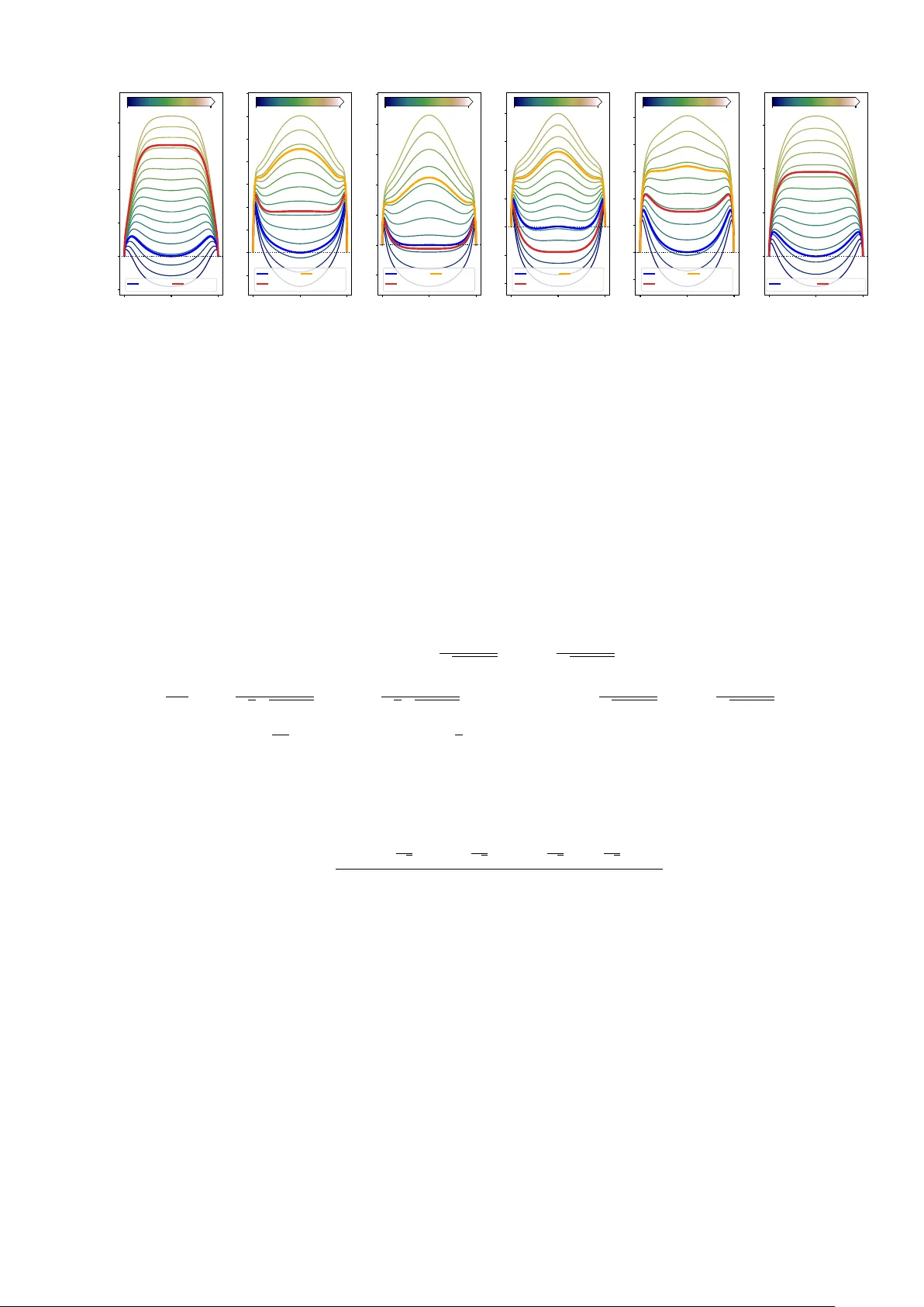
The Symmetric P erceptron: a T eac her-Studen t Scenario Gio v anni Catania, 1, 2 Aurélien Decelle, 1, 3, 4 and Suhanee K orp e 1, 5 , ∗ 1 Dep artamento de Físic a T e óric a, Universidad Complutense de Madrid, 28040 Madrid, Sp ain 2 Institute for Cr oss-disciplinary Physics and Complex Systems IFISC (CSIC-UIB), Campus Universitat Il les Bale ars, 07122 Palma de Mal lor c a, Sp ain. 3 Université Paris-Saclay, CNRS, INRIA T au te am, LISN, 91190 Gif-sur-Yvette, F r anc e. 4 GISC - Grup o Inter disciplinar de Sistemas Complejos 28040 Madrid, Sp ain. 5 Indian Institute of Scienc e Educ ation and R ese ar ch, Bhop al 462066, India W e in tro duce and solv e a teacher-studen t form ulation of the symmetric binary P erceptron, turning a traditionally storage-oriented mo del into a planted inference problem with a guaranteed solution at any sample density . W e adapt the formulation of the symmetric Perceptron which traditionally considers either the u-shap ed p otential or the rectangular one, by including lab els in b oth regions. With this formulation, we analyze b oth the Bay es-optimal regime at for noise-less examples and the effect of thermal noise under tw o different potential/classification rules. Using annealed and quenc hed free-entrop y calculations in the high-dimensional limit, we map the phase diagram in the three control parameters, namely the sample density α , the distance b etw een the origin and one of the symmetric h yp erplanes κ and temperature T , and identify a robust scenario where learning is organized by a second-order instability that creates teacher-correlated sub optimal states, follo wed b y a first-order transition to full alignment. W e show how this structure dep ends on the choice of p oten tial, the interpla y b etw een metastability of the sub optimal solution and its melting to wards the planted configuration, which is relev ant for Monte Carlo-based optimization algorithms. I. INTR ODUCTION The Perceptron [ 1 ] is the simplest sup ervised classification mo del and plays a dual role: it constitutes a foundational elemen t of mo dern deep-learning architectures [ 2 ] and provides a paradigmatic framew ork for analyzing learning dynamics [ 3 , 4 ] and applying statistical-mechanics techniques to learning problems [ 5 ]. Since Gardner’s seminal work on the storage capacity of the spherical Perceptron [ 6 ], and the w ork by Krauth & Mezard on its binary v ersion [ 7 ] a large b o dy of research has explored its thermo dynamic prop erties, phase transitions, and algorithmic b eha vior using to ols originally developed for disordered systems [ 8 – 11 ]. In particular, the teacher-studen t (TS) setting [ 5 , 12 ] has emerged as a natural framew ork to study learning as an inference problem, where a student mo del attempts to reco ver a hidden teac her [ 13 , 14 ] from lab eled examples generated according to the same rule [ 15 , 16 ]. In this work, we fo cus on a symmetric v ersion of the binary P erceptron in a TS setting, where the solution space is symmetric under the in v ersion of the weigh t vector. Unlik e the standard Perceptron, whose decision boundary is a single h yp erplane, the symmetric Perceptron is in v arian t under a global sign flip of the weigh ts, leading to a classification rule defined by tw o symmetric hyperplanes, the distance of which is tuned by the so-called margin parameter κ . This symmetry in tro duces a ric her structure in the space of solutions and naturally gives rise to multiple comp eting phases. Symmetric versions of the P erceptron hav e previously b een studied mainly in the context of storage problems with prescrib ed lab el distributions, often using u-shap ed or rectangular p otentials [ 17 , 18 ]. Here, we adapt this framew ork to the TS scenario by explicitly incorp orating teacher-generated lab els in b oth regions defined by the symmetric decision rule. T o our kno wledge, an analytic mean-field c haracterization of this mo del in the TS setting, including the full phase-diagram structure — in terms of the three control parameters, namely the sample densit y α , the margin parameter κ and temp erature T — has not b een rep orted previously . As w e show, this discrete symmetry qualitativ ely c hanges the learning landscape: it can separate the onset of non-zero but sub-optimal correlations to wards the teacher from full teacher recov ery , pro ducing a characteristic second-order/first-order sequence of transitions. Our analysis combines annealed and quenched calculations of the free entrop y in the high-dimensional limit, using the replica metho d under a replica-symmetric ansatz [ 8 ]. W e inv estigate b oth a piecewise constan t loss, analogous to the original formulation studied b y Gardner, and a linear loss that p enalizes misclassified samples prop ortionally to their distance from the decision b oundary [ 3 ]. This allows us to characterize not only the Bay es-Optimal (BO), zero-temp erature regime—where the student p erfectly matches the teacher—but also the effects of thermal noise and finite temp erature learning dynamics. ∗ suhanee21@iiserb.ac.in 2 Our goal is to characterize the phase diagram of the symmetric binary Perceptron as a function of the sample density α , the margin κ , and the temp erature T . T o this end, we compute the relev ant transition lines — first- and second- order transitions as well as spino dal p oints of the sub-optimal/optimal solution — that determine when information ab out the teacher b ecomes accessible and when full reco very is thermo dynamically fav ored. W e also identify a phase c haracterized by metastable, sub optimal states, in which the system admits solutions that are uncorrelated or partially correlated with the teac her. These transitions control the onset of learning, the developmen t of correlations with the teac her, and the stability of paramagnetic and glassy phases. By systematically comparing different p otentials and temp eratures, we obtain a comprehensive thermo dynamic picture of learning in symmetric Perceptron mo dels. This pap er is organized as follows, in Section II, w e in tro duce the symmetric binary Perceptron mo del under the TS setting and the t wo p otentials, namely the constan t and the linear potentials, under whic h we study the mo del. Next, in Section I I I, we b egin our analysis b y presen ting the annealed computation for the constant p otential. W e provide the expressions for the free energy and the corresp onding saddle-point equations. W e also present the free-energy profiles that clearly depict the phase transitions, spino dal, first-order, and second-order, for different v alues of α and κ at T = 0 , and summarize the resulting phase b ehavior. T o obtain a more rigorous description, we then present the quenched computations and results in Section IV. In particular, w e analyze the Bay es-optimal case and consider b oth p oten tials at finite temp erature. W e show the free-energy profiles for the Bay es-optimal case by v arying α and κ and compare the ( T , α ) phase diagrams for the constant and linear p otentials. Finally , we conclude by summarizing our results and discussing p ossible extensions and future directions of this work. W e provide detailed calculations in the app endices. In App endix A, we present the deriv ation of the annealed disorder computation. In App endix B, we pro vide the quenc hed analysis, with three subsections deriving the results for the Bay es-optimal case, the constant p oten tial, and the linear p otential, resp ectively . I I. DEFINITION OF THE MODEL The classical binary Perceptron formulation consists of classifying a set of M binary examples ξ µ , where each sample liv es in a N − dimensional h yp ercub e ξ µ ∈ {− 1 , 1 } N . In our analysis, we consider the high-dimensional regime where the num b er of samples M scales with the system size N , such that α = M /N ∼ O (1) as M , N → ∞ . The output of a P erceptron is typically considered to b e generated b y the (noise-less) learning rule σ µ = sign( w · ξ µ ) , where σ µ is the output that takes binary v alues {− 1 , 1 } . Geometrically , this implies that a single hyperplane orthogonal to w separates the data p oints in to tw o classes. In the context of a TS scenario, the lab els of the samples are generated b y a teacher P erceptron with a weigh t vector w 0 , whose comp onents are assumed to b e i.i.d. binary v ariables w 0 i ∈ {− 1 , 1 } . The studen t Perceptron learns its weigh ts w using the training sample ξ µ and its corresp onding lab el σ µ 0 generated by the teac her, according to σ µ 0 = sign( w 0 · ξ µ ) . (1) In practice, the lab el is determined by the datum’s p osition relativ e to the separating hyperplane defined b y the teac her. In this pap er, we consider a symmetric version of the Perceptron where if w is a solution to our problem, that is, it classifies all samples correctly , then so is w ′ = − w . This choice symmetrizes the mo del, so that the configuration space is now cut by t w o hyperplanes, defined by κ + w · x = 0 and κ − w · x = 0 , where κ represents the shift of the hyperplane from the origin. In such a case, the Hamiltonian will b e symmetric under the transformation w → − w . A simple visualization of the decision boundary in the symmetric Perceptron for a 2-dimensional mo del ( N = 2 ) is given in Fig. 1 . In the storage formulation, the fundamental question that is addressed is usually ab out the volume of samples that can be classified correctly , given a (typically random) set of M examples, from which the critical capacit y is computed and corresp onds to a SA T-UNSA T transition in the jargon of constraint satisfaction [ 17 – 19 ]. A t ypical choice for theoretical computation is to use random samples and random lab els that can b e contained inside or outside the area delimited by b oth hyperplanes. In the TS formulation [ 9 , 12 ], w e hav e at our disp osal a teac her that generates the lab els, thereb y ensuring that a solution to the problem exists, regardless of the num ber of samples. In the TS formulation, and in the absence of external thermal noise (i.e., at T = 0 ), the teacher guaran ties satisfiability for any α , so the central question b ecomes when the Gibbs measure acquires non-trivial o verlap with the teacher and ho w metastability can obstruct algorithmic reco very . Let us now formalize the symmetric Perceptron mo del. W e can first define a loss function that will, given the lab els of the system and the w eights w , count how many samples are misclassified. The Hamiltonian, or training loss 3 − 2 − 1 0 1 2 − 2 0 2 − 1 1 − 1 FIG. 1. Decision boundary for a symmetric P erceptron in N = 2 with w =  − 1 / √ 2 , 1 / √ 2  and κ = 1 , illustrating a case where the data in the red region are lab elled +1 , while the ones in the blue region are lab eled − 1 . function, asso ciated with the studen t can b e written in the following form H [ w | ξ , w 0 ] = M X µ =1 V ( ω µ , σ µ 0 ) , (2) where we used the notation ω µ = ξ µ · w where ξ denotes the set of patterns ξ µ , µ = 1 , . . . , M and w 0 the teacher’s w eight with σ µ 0 giv en by the decision b oundary of the teacher’s weigh ts as i n Fig. 2 . In practice, if the lab el of a sample is σ 0 = 1 , it should lie inside the hyperplanes defined by the teac her, while in the case σ 0 = − 1 , it should lie outside, as illustrated in Fig. 2 . When fo cusing only on correctly classifying all the lab els, it is enough to just count the n umber of errors. In a statistical ph ysics’ context, it is also common to consider the finite temp erature b ehaviour, b y defining the Gibbs-Boltzmann distribution p ∝ exp( − β H ) of the system to analyse how entropic contribution can comp ete with the minimization of the cost function. T o extend our analysis to the finite temp erature of such ob ject, w e considered tw o different defini tions of the Hamiltonian that are equiv alent in the limit β − 1 = T → 0 . First, we will consider the piecewise constant p otential whic h assigns a constant cost to incorrectly classified samples as shown in Fig. 2 left panel. The analytical formulation of the p oten tial is given by V (0) ( ω , σ 0 ) = ( Θ [ − ω − κ ] + Θ [ ω − κ ] , if σ 0 = 1 , Θ [ κ + ω ] Θ [ κ − ω ] , if σ 0 = − 1 . (3) In this case, any misclassified sample suffers the same unit error: this is typically referred to as the Gibbs learning rule [ 3 , 6 ]. Despite the known problem with the frozen dynamics of suc h p otential [ 20 ], w e consider it to b e m uch easier to deal with in order to solve numerically the phase diagram ov er the entire temp erature range. The second Hamiltonian we consider contains a linear p oten tial whic h assigns a linear cost to the incorrectly classified data p oin ts as shown in Fig. 2 right panel, similarly to the one studied in [ 9 ], which leads to a smo other energy landscap e. The form of the linear p otential is given b elow V (1) ( ω , σ 0 ) = ( ( − ω − κ ) Θ [ − ω − κ ] + ( ω − κ ) Θ [ ω − κ ] , if σ 0 = 1 , ( κ − | ω | ) Θ [ κ + ω ] Θ [ κ − ω ] , if σ 0 = − 1 . (4) This p otential follows the traditional P erceptron cost function [ 3 ] in which misclassified samples that are far aw ay from the decision boundary are penalized more strongly . This potential is more suitable for Mon te Carlo based optimization, giv en its informativ e p otential, it is also exp ected, that when using the constant piece-wise p otential V (0) , the dynamics will be frozen due to entropic barriers, while in the case of linear p otential, it is exp ected that for a large num b er of data, an y lo cal dynamics could find easily a solution [ 20 , 21 ]. This comparison isolates whic h features of the phase diagram are in trinsic to the symmetric decision rule and which depend on the smo othness of the optimization landscap e induced by the choice of the loss. In order to characterize the phase diagram of the symmetric binary Perceptron, w e use the replica approac h to implemen t the mean field theory , [ 6 , 8 , 22 ] to compute the partition functions and free energies for b oth the p otentials, as a function of the inv erse temp erature β , the num b er of sam ples α and the width κ of the p otential Z [ ξ , w 0 ] = X w = {± 1 } N exp  − β H [ w | ξ , w 0 ]  . (5) 4 0 1 V (0) ( ω , + ) V (0) − 2 − 1 0 1 2 ω /κ 0 1 V (0) ( ω , − ) 0 1 V (1) ( ω , + ) V (1) − 2 − 1 0 1 2 ω /κ 0 1 V (1) ( ω , − ) FIG. 2. Left: the p oten tial V (0) for b oth lab els σ 0 = ± 1 . With this p oten tial, any error has a fixed cost. Right: the linear p otential V (1) for b oth lab els σ 0 = ± 1 . This p otential tends to p enalize more errors that are far aw ay from the decision b oundary . where the studen t’s w eigh ts are summed o v er all possible v alues. In the rest of the pap er, w e will consider that the comp onents ξ µ i of the dataset and the teacher weigh ts w 0 i will b e distributed uniformly in in {± 1 } with equal probabilit y p = 1 / 2 , and denote the av erage ov er it as E D [ . ] for the dataset and E w 0 [ . ] for the teacher’s weigh t vector. I I I. ANNEALED FREE ENERGY COMPUT A TION FOR THE PIECE-WISE POTENTIAL In order to understand the physics of the mo del, we provide an analysis of the annealed computation of the free entrop y for the Hamiltonian with the piece-wise constant p otential. In the annealed approximation, instead of computing the disorder-a verage of the logarithm of the partition function, we tak e the logarithm of the a verage of the partition function. Already at T = 0 , the annealed theory reveals a co existence structure in the o verlap b et ween equilibrium configurations and the teacher’s w eights that explains why teacher recov ery can b e discontin uous and is preceded b y an extensive regime in α where sub optimal minima dominate the thermo dynamics. In the following, w e will denote the disorder a v eraged on the dataset as E D and the av erage o v er the teac her w eigh ts as E w 0 . In the thermo dynamic limit, the expression of the free energy , denoted by G is giv en by −G ( κ, α ) annealed = lim N →∞ 1 N log E D , w 0  Z [ ξ , w 0 ]  , (6) where the dataset is D = { ξ µ } M µ =1 , and we analyze the free energy as a function of the margin κ , the inv erse temperature β and the ratio of the num b er of samples and features α . W e put details of the computation in App endix A . T o explain the computation in brief, we introduce the order parameter R = 1 N N X i w i w 0 i (7) represen ting the o verlap b etw een the studen t and the teac her. A v alue R ∼ 0 means that there is no correlation b et ween the teacher and the studen t while R = 1 means the student has found the teac her configuration. When in tro ducing this parameter, the free energy density as decomp oses as given b elow −G = − R ˆ R + G S ( ˆ R ) + α G E ( R ) (8) where ˆ R is the conjugate ov erlap parameter, G S is the en tropic contribution, counting the volume of weigh t con- figurations at fixed ov erlap, and G E is the energetic contribution, which is the av erage training cost per example at a fixed student-teac her ov erlap, representing ho w well a student aligned with the teacher satisfies the constrain ts. Learning is gov erned by a trade-off b etw een en tropy , which fa vors many compatible weigh t configurations, and energy , whic h p enalizes configurations that p o orly satisfy the training constrain ts. While op ening the Hamiltonian V (∆ µ ) in the energetic part, w e split the ∆ -in tegral into disjoint regions according to whether | ∆ | > κ or | ∆ | ≤ κ , yielding 5 − 1 0 1 R − 0 . 2 0 . 0 0 . 2 0 . 4 0 . 6 0 . 8 f κ = 0 . 5 α = 1 . 08 α = 2 . 13 − 1 0 1 R − 0 . 02 0 . 00 0 . 02 0 . 04 0 . 06 0 . 08 0 . 10 0 . 12 0 . 14 κ = 0 . 9 α = 1 . 11 α = 1 . 17 α = 1 . 25 − 1 0 1 R − 0 . 05 0 . 00 0 . 05 0 . 10 0 . 15 0 . 20 0 . 25 κ = 1 . 0 α = 1 . 22 α = 1 . 21 α = 1 . 42 − 1 0 1 R − 0 . 10 − 0 . 05 0 . 00 0 . 05 0 . 10 0 . 15 0 . 20 κ = 1 . 25 α = 1 . 71 α = 1 . 60 α = 2 . 03 − 1 0 1 R − 0 . 05 0 . 00 0 . 05 0 . 10 0 . 15 0 . 20 0 . 25 κ = 1 . 8 α = 4 . 84 α = 5 . 36 α = 5 . 95 − 1 0 1 R 0 . 0 0 . 2 0 . 4 0 . 6 κ = 2 . 2 α = 12 . 47 α = 19 . 41 0 . 8 2 . 4 α 1 . 06 1 . 30 α 1 . 1 1 . 6 α 1 . 45 2 . 20 α 4 . 4 6 . 6 α 10 24 α ( a ) ( b ) ( c ) ( d ) ( e ) ( f ) FIG. 3. Snapshots of free energy profiles at 6 differen t v alues of κ , corresp onding to the thin v ertical lines in Fig. 4 (left panel). Eac h panel ( a ) → ( f ) shows sev eral free energy profiles f ( R ) at differen t v alues of α . The thick er curves corresp ond to the v alues of the first/second order transition and the spino dal (when differen t). In blue we illustrate first order transitions, in red second order ones and in y ellow the melting (spinodal) point of the sub-optimal solution 0 < R < 1 . The colors used here are the same as in Fig. 4 . separate Gaussian contributions from the inactive and active regions, resp ectiv ely , the latter acquiring an additional Boltzmann weigh t e − β . Ev aluating these pieces explicitly leads to the decomp osition of the free energy in tegral. W e obtain the free energy of the system by considering the saddle p oin t of the free energy parameterized b y the order parameter R and its conjugate parameter ˆ R . The saddle-p oint solution reflects a comp etition b etw een the entropic term and the energetic term. The precise deriv ation of the annealed free energy is given in the App endix A . In order to find the equilibrium of the mo del in the thermo dynamic limit, we determine the minima of this free energy by solving n umerically the self-consistent saddle p oint equations (( A6 ) and ( A15 ) given in App endix A ). In this approximation, the expression for the free energy is given by −G = − R ˆ R + ln 2 cosh ˆ R + α ln  2 Z ∞ κ D u  Φ  κ − uR √ 1 − R 2  + Φ  κ + uR √ 1 − R 2  + Z κ − κ D u 2  erf  κ + uR √ 2 √ 1 − R 2  + erf  κ − uR √ 2 √ 1 − R 2  + 2 Z κ − κ D u  Φ  κ − uR √ 1 − R 2  + Φ  κ + uR √ 1 − R 2  e − β  , where D u = exp( − u 2 / 2) / √ 2 π du and Φ( x ) = erfc( x/ √ 2) / 2 . W e exp ect that due to the symmetry of the model, the annealed computation exhibits b oth a kind of paramagnetic phase where no signal can b e detected in the equilibrium measure and th us R = 0 , and a phase where, when enough samples are pro vided the system is capable of retrieving at least partially the teacher R ≥ 0 . In such scenario, we can inv estigate analytically the stability of the paramagnetic solution, and w e found that it is stable up to α (2) c = π  erfc 2 ( κ √ 2 ) + erf 2 ( κ √ 2 ) + 2 erf ( κ √ 2 ) erfc ( κ √ 2 ) e − β  4 e − κ 2 κ 2 (1 − e − β ) , (9) where a second order phase transition would take place. How ev er, the mo del exhibits a richer phenomenology due to a phase co existence betw een the aforemen tioned paramagnetic state or a sub optimal solution with 0 < R < 1 and the teacher configuration R = 1 . The k ey qualitative p oin t is that the free-energy landscap e can develop three comp eting minima (paramagnetic, sub optimal correlated, and teacher), whose crossings generate first-order lines and whose disapp earances define spino dal p oin ts. T o ha ve a clearer understanding, we summarize in Fig. 3 six different free-energy profiles as a function of R at differen t v alues of k (one profile per each panel) and v arying the fraction of samples α av ailable to the students (differen t v alues of α are shown in each panel where α increases from blue-ish to yello w-ish colors). F or small v alues of κ , (see e.g the left-most panel κ = 0 . 5 ) and v arying the density of samples α , the system exhibits a first order phase transition at α (1) c ( α (1) c ≈ 1 . 08 in Fig. 3 -( a )) from a paramagnetic regime R = 0 , to w ards a system fully polarized to wards the teacher, i.e R = 1 . This crossing identifies the first-order transition: at α (1) c the global minimum jumps from R = 0 to R = 1 while the paramagnetic state remains locally stable up to its spino dal p oint. Of course, the 6 0 . 5 1 . 0 1 . 5 2 . 0 κ 10 0 10 1 α Annealed 1st-order PT Spinodal 2nd-order PT 0 . 5 1 . 0 1 . 5 2 . 0 κ 10 0 10 1 α Quenc hed Spinodal 1st Order PT 2nd-order PT FIG. 4. Left: Phase diagram of the symmetric binary Perceptron at T = 0 , using the annealed approximation. Right: Phase diagram of the symmetric binary P erceptron at T = 0 , using the quenched approximation in the Bay es-Optimal setting. The v ertical lines indicate the v alues of κ used on Fig. 3 (resp. Fig. 5 ) for the annealed (resp. quenched) case. In b oth cases, the blue line indicated the first order transition, the red line the second order one and the yello w line the spino dal, that is when the sub-optimal solution disapp ear. In the range of κ where the second order phase transition o ccurs, the dashed-blue line only corresp onding to when the unstable paramagnetic state and the teacher state hav e the same free energy . teac her is in practice unreachable unless the system is initialized close to it in that regime: indeed, the paramagnetic solution remains stable for quite large v alues of α ∼ 2 . 13 (giv en b y Eq. 9 ) un til it melts tow ard the teac her. Therefore, this second threshold of α (red line in Fig ( 3 )) marks the spino dal p oint of the paramagnetic solution. Increasing κ mo difies the phenomenology of the mo del. F or a v alue of κ = 0 . 9 (depicted in Fig. 3 -( b )), after undergoing the first order transition at α (1) c ∼ 1 . 11 , the lo cally stable paramagnetic solution is split, undergoing a second order phase transition (thick red line in Fig. 3 ), into tw o (symmetric) sub optimal solutions but with a large ov erlap with the teac her R > 0 . In this case at α (2) c ∼ 1 . 17 , the second order phase transition now tak es place within the sub dominant paramagnetic. A t higher v alues of α , the tw o sub optimal solutions finally melt tow ard the teacher at α ∼ 1 . 25 (thick orange line). In another in termediate regime at higher v alues of κ , e.g in panels ( c )-( d ), the second order phase transition o ccurs b efore the first order one. In panel ( e ) the phenomenology is the same as in ( b ). Finally , increasing further κ restores the initial b eha vior: e.g. at κ = 2 . 2 (panel ( f )), the situation go es bac k to the extremely small- κ case, with a first order transition taking place b eforehand and no sub optimal solution with 0 < R < 1 exists at an y v alue of α . W e summarize these differen t phases in Fig. 4 (left panel), where we show the v arious critical lines in the ( κ − α ) plane at temperature T = 0 . The 3-phases regime with a sub-optimal solution 0 < R < 1 exists for intermediate v alues of κ , whose spino dal p oin t is depicted in Fig. 4 as an orange line. F rom a numerical p oint of view, the 1 − st order phase transition (blue lines) is computed for a fixed κ and v arying α by lo oking at the p oint where the free energy of the sub-optimal solution (or the paramagnetic one) b ecomes p ositive (i.e larger than the teacher’s one which is n ull). Similarly , the spino dal line corresp onds to the p oint at which starting from an initial condition R ≈ 0 the saddle p oint equation conv erges to the teacher R = 1 . The co de used to generate the critical lines in Fig. 3 (and the other phase diagrams shown in the next section) is included in a op en-access rep ository [ 23 ]. IV. QUENCHED FREE ENERGY COMPUT A TION W e no w turn our analysis tow ards the quenched free energy for the mo del defined b y Eq. ( 5 ). The main thermo- dynamic quantit y pro viding information ab out the system is the quenched av erage of the free energy density , given b y −G ( κ, α, β ) = lim N →∞ 1 N E D , w 0 log Z . (10) 7 0 . 0 0 . 5 1 . 0 R − 0 . 5 0 . 0 0 . 5 1 . 0 1 . 5 2 . 0 f κ = 0 . 3 0 . 0 0 . 5 1 . 0 R − 0 . 1 0 . 0 0 . 1 0 . 2 0 . 3 κ = 0 . 8 0 . 0 0 . 5 1 . 0 R − 0 . 2 − 0 . 1 0 . 0 0 . 1 0 . 2 0 . 3 κ = 0 . 9 0 . 0 0 . 5 1 . 0 R − 0 . 3 − 0 . 2 − 0 . 1 0 . 0 0 . 1 0 . 2 0 . 3 κ = 1 . 0 0 . 0 0 . 5 1 . 0 R − 0 . 25 − 0 . 20 − 0 . 15 − 0 . 10 − 0 . 05 0 . 00 0 . 05 0 . 10 κ = 1 . 2 0 . 0 0 . 5 1 . 0 R − 0 . 4 − 0 . 2 0 . 0 0 . 2 0 . 4 0 . 6 0 . 8 1 . 0 1 . 2 κ = 1 . 5 0 . 8 4 . 0 α 0 . 8 1 . 4 α 0 . 8 1 . 4 α 0 . 6 1 . 4 α 0 . 8 1 . 4 α 0 . 8 4 . 0 α ( a ) ( b ) ( c ) ( d ) ( e ) ( f ) FIG. 5. Snapshots of free energy profiles at 6 different v alues of κ at T = 0 in the Ba yes-Optimal setting. W e can observe a phase diagram that is qualitatively similar to the annealed case. F rom small v alues of κ , we observe first a first order phase transition, follow by a melting tow ard the teacher state at higher v alues of α . Then, w e hav e the at larger κ a second order phase transition b efore the melting. The quenc hed computation is essential in the TS setting b ecause it determines which teacher-correlated states domi- nate in the typic al case, b eyond the optimistic annealed picture. T o calculate the exp ectation of the logarithm of the partition function, w e use the replica trick, which in volv es introducing n replicas and using the following identit y ⟨ log Z ⟩ = lim n → 0 ⟨Z n ⟩ − 1 n (11) By using the replica trick, we end up defining the usual order parameters R a = 1 N N X i w a i w 0 i (12) q ab = 1 N N X i w a i w b i , (13) represen ting resp ectively the ov erlap b etw een the student and the teacher and the ov erlap b etw een different students. The first parameter R a has the same interpretation as in the annealed case, while the second parameter q ab is the o verlap betw een t wo replicas a and b , indicating the presence of p oten tially glassy states. In general, as in the annealed case, the parameter R a indicates the ov erlap with the teacher, and R a ∼ 1 means that the system has found the optimal solution. In such a case, we also hav e that q ab ∼ 1 . A glassy state is detected b y b oth a n ull ov erlap with the teac her R a ∼ 0 , while the o v erlap b etw een tw o studen ts is differen t from zero q ab  = 0 . In order to find the equilibrium of the mo del in the thermodynamic limit, w e assume the replica symmetric (RS) ansatz R = R a and q = q ab ∀ replicas a and b , and pro ceed similarly to the annealed case. In this work, w e obtain the free energy of the system b y considering the saddle p oint of the free energy parameterized b y the order parameters in the RS approximation. In this section, we first start by analyzing the Ba yes-Optimal (BO) results, and finally , w e discuss the b eha vior in temp erature of the tw o different Hamiltonians. A. The Bay esian-Optimal case The Bay es-Optimal scenario, corresp onds to the limit of zero temp erature ( T = 0 ) where the studen t mo del p erfectly matc hes the teacher’s learning algorithm. As established in the analysis of the classical Perceptron [ 3 ], this condition significan tly simplifies the computation. The system is constrained to the Nishimori line [ 5 ], where the o verlap b et ween t wo replicas of the studen t ( q ) b ecomes identical to the o verlap b etw een the studen t and the teacher ( R ). 8 Consequen tly , setting q = R in the replica symmetric ansatz yields the following simplified free energy , −G = − ˆ R 2 ( R + 1) + Z D z ln 2 cosh ( p ˆ Rz + ˆ R ) + α ×  Z D t [Φ ( A + ) + Φ ( A − )] log { [Φ ( A + ) + Φ ( A − )] } + Z D t  1 2 erf  A + √ 2  + 1 2 erf  A − √ 2  log  1 2 erf  A + √ 2  + 1 2 erf  A − √ 2  with A ± = κ ± √ Rt √ 1 − R (14) and Φ( x ) = 1 2 erfc ( x √ 2 ) . In this regime, the only order parameter is therefore given by R = Z D z tanh 2  p ˆ Rz + ˆ R  and the expression for the conjugate parameter ˆ R can be found in App endix B2 . W e can fully appreciate the different phase to which the system go es through as the parameter α is changed and for v arious v alues of κ . Similar to the annealed case, we can compute the threshold up to which the paramagnetic solution is stable, given b y the follo wing form ula: α (2) c = π 2 κ 2 e κ 2 erf  κ/ √ 2  erfc  κ/ √ 2  . (15) The main difference w.r.t. the annealed case is that now the sub-optimal solution 0 < R < 1 seems to alwa ys exist for κ larger than a threshold identified by the p oint where the orange and red lines in Fig. 4 start to ha ve different v alues. B. Beha vior in temp erature W e finally exhibit the b ehavior of the system at finite temp erature. In this case, both potentials are exp ected to exhibit different b ehaviors. W e direct the reader to App endix B1 and B3 for the detailed computation and only write the functional form of the free energy for b oth p otentials here. F or the p oten tial V (0) w e obtain 1 n log G E = Z D t [Φ ( A + ) + Φ ( A − )] log  2 [Φ ( B + ) + Φ ( B − )] + e − β  erf  B + √ 2  + erf  B − √ 2  + + Z D t  1 2 erf  A + √ 2  + 1 2 erf  A − √ 2  log  2 e − β [Φ ( B + ) + Φ ( B − )] + erf  B + √ 2  + erf  B − √ 2  , (16) with A ± = κ √ q ± R t p q − R 2 and B ± = κ ± √ q t √ 1 − q . (17) W e clearly see how the Boltzmann factor e − β con tributes to an extra term in the free energy that tak es into account the possibility to commit an error p enalized by a weigh t β . It is possible to compute the instabilit y of the paramagnetic solution at all temp eratures and v alues of κ , thanks to the spin-flip symmetry of the problem. T o do that, we expand the free energy around R = 0 and lo ok for the p oin t when its second deriv ative computed in R = 0 changes sign. F or this p otential, we find that the instability is given by α (0) 2 nd ( β , κ ) = e κ 2 π h erf  κ √ 2  + e − β erfc  κ √ 2 i h e − β erf  κ √ 2  + erfc  κ √ 2 i 2 κ 2 (1 − e − 2 β ) (18) from which we reco ver the case of the BO case in the limit β → ∞ . The free energy in the case of the V (1) p oten tial tak es the following form 9 1 n log G E = Z D t [Φ ( A + ) + Φ ( A − )] log  [Φ ( B + ) + Φ ( B − )] + e − β κ + β 2 (1 − q ) 2 P 1  + + Z D t  1 2 erf  A + √ 2  + 1 2 erf  A − √ 2  log  e β κ + β 2 (1 − q ) 2 P 2 + 1 2 erf  B + √ 2  + 1 2 erf  B − √ 2  , (19) P 1 = 1 2 e − β √ q t  erf  B − ( κ ) √ 2  − erf  B − (0) √ 2  + 1 2 e β √ q t  erf  B + (0) √ 2  − erf  B + ( − κ ) √ 2  , (20) P 2 = 1 2 e β √ q t erfc  B + ( κ ) √ 2  + 1 2 e − β √ q t erfc  − B − ( − κ ) √ 2  . (21) In this expression, the temp erature dep endent terms are now more complicated, since they hav e to take into account the distance from the decision b oundary . The computation in this case of the instability is more inv olved, yet it can b e analytically done and yields 1 α (1) c = e − κ 2 κβ  2 e β 2 2 erf  κ − β √ 2  + 2 e β 2 2 erf  β √ 2  + erf  κ √ 2   2 e κ 2 2 − 2 e κβ + e 1 2 ( κ 2 + β 2 ) √ 2 π β erf  κ − β √ 2  + e 1 2 ( κ 2 + β 2 ) √ 2 π β erf  β √ 2  +2 e κβ erfc  κ √ 2  + 2 e 1 2 ( κ + β ) 2 erfc  κ + β √ 2  − 2 e 1 2 β (4 κ + β ) erfc  κ + β √ 2  − − e 1 2 ( κ 2 +4 κβ + β 2 ) √ 2 π β erfc  κ √ 2  erfc  κ + β √ 2  /  π  e β 2 2 erf  κ − β √ 2  + e β 2 2 erf  β √ 2  + e κβ erfc  κ √ 2   erf  κ √ 2  + e 1 2 β (2 κ + β ) erfc  κ + β √ 2  . (22) T ak en together, Eqs. ( 18 ) and ( 22 ), these expressions sho w that temp erature do es not merely smear transitions; it reshap es the stability of the R = 0 phase in a loss-dep endent w ay , thereb y con trolling whether learning b egins con tinuously or only via a discontin uous jump. In the follo wing, we provide the full phase diagram in the α − T plane of the system for the sp ecific case κ = 1 . On Fig. 6 (left), we plot the different lines of transitions. W e can see that for T < 0 . 7 , by increasing α we gradually pass from a paramagnetic regime q = R = 0 where the teacher do es not exist tow ard first, the teacher appearing (teac her spino dal line), then a second order phase transition where the paramagnetic state splits in to t wo sub-optimal states, then a first order transition where the teacher state becomes dominan t to end up with the melting of the sub-optimal states. F or high temp erature, the first and second order transitions are in verted as can b e seen. At the dynamical level, it is exp ected that the system is frozen, as already seen for the piece-wise p otential of the usual P erceptron [ 20 ]. On Fig. 6 (right), we plot the same kind of figure when considering the p oten tial V 1 . In this phase diagram, we qualitatively reco ver the part of the same physics as the classical P erceptron. The main difference no w is that a second order transition makes its app earance, and thus the system, for sufficiently high temp eratures, remains trapp ed in a paramagnetic state R = 0 until it crosses the second order phase transition. V. CONCLUSIONS In this pap er, w e hav e presen ted a statistical-mechanical analysis of the symmetric binary P erceptron in a TS scenario. By extending the traditional form ulation of the symmetric Perceptron to explicitly include teacher-generated lab els, w e were able to study learning as an inference problem rather than a pure storage task. This distinction ensures the existence of a solution for all sample densities and shifts the fo cus to the nature of conv ergence tow ard the teacher as the amoun t of data (here tuned by the parameter α in the thermo dynamic limit) increases. Our cen tral finding is that the sign symmetry generically splits learning into tw o stages: the app e ar anc e of teacher correlation via a second-order instabilit y and the sele ction of the teacher via a first-order transition, with a metastable regime in b et ween. Using b oth annealed and quenched free entrop y calculations, we characterized the phase structure of the mo del in the thermo dynamic limit. In the Bay es-optimal, zero-temp erature regime, we found that learning can pro ceed through a sequence of phase transitions whose order dep ends sensitively on the margin κ . In particular, the system ma y exhibit a second-order transition from a paramagnetic phase to sub optimal states with finite ov erlap with the 10 0 . 8 1 . 0 1 . 2 1 . 4 1 . 6 1 . 8 2 . 0 2 . 2 α 0 . 0 0 . 1 0 . 2 0 . 3 0 . 4 0 . 5 0 . 6 0 . 7 0 . 8 T κ = 1 α 2nd c 2ndO PT 1stO PT SupOpt Spinodal ( a ) 0 . 4 0 . 6 0 . 8 1 . 0 1 . 2 1 . 4 1 . 6 α 0 . 00 0 . 05 0 . 10 0 . 15 0 . 20 0 . 25 T κ = 1 T eacher Spino dal 2ndO PT 1stO PT SupOpt Spinodal ( b ) FIG. 6. Left: Phase diagram of the constant p otential V 0 at κ = 1 . Righ t: Phase diagram of the piece-wise constant potential V 1 at κ = 1 . As in the case of the P erceptron, the orange line is exp ected to terminate at (0 , 0) . In this parameter regime, the shap e of the p otential strongly influences the structure of the loss landscap e. F or V 0 , and for sufficiently large T and α , there exists a phase in which the teacher dominates the equilibrium measure, while a typical exp eriment remains trapp ed in completely uncorrelated states. In contrast, for V 1 , the second-order phase transition is alwa ys dominant with resp ect to the other transitions and provides information ab out the teacher well before the latter even becomes a metastable state. teac her, follow ed by a first-order transition tow ard full alignment. This b ehavior highlights the nontrivial role play ed b y symmetry and margin constraints in shaping the learning landscap e. A t finite temperature, the phenomenology becomes even ric her. F or the piecewise constan t p otential, thermal fluctuations introduce additional metastabilit y and spino dal lines, reminiscen t of the frozen dynamics observ ed in earlier studies of the Perceptron [ 20 ]. In contrast, the linear p otential leads to smo other energy landscap es and phase diagrams that more closely resemble those of the classical P erceptron, while still retaining signatures of symmetry- induced transitions absent in the standard mo del. Our results show that the choice of loss function has a qualitative impact on b oth the thermo dynamic phases and the expected dynamical b ehavior of learning algorithms. This ther- mo dynamic organization provides a direct mechanism for algorithmic v ariability: lo cal dynamics can remain trapp ed in sub optimal teac her-correlated states up to spino dals, while smo other losses can reduce barriers without removing the underlying symmetry-driv en transition structure. While our analysis is p erformed within the replica symmetric approximation, one can already anticipate that, in the T = 0 regime, the easy–hard algorithmic threshold is connected to instabilities of the RS solution, namely to the de Almeida–Thouless line [ 24 ], in close analogy with the (classical) Perceptron case. Indeed, at T = 0 computations are carried out in the Bay es-optimal regime, and the emergence of sub optimal solutions is typically asso ciated with the failure of m essage-passing algorithms to conv erge, which in turn signals the onset of the A T instability . Ov erall, this work provides an integrated p ersp ective on the in terplay b etw een symmetry in the decision b oundary , margin constrain ts, and noise in high-dimensional learning problems. Although w e fo cus on a to y mo del, the symmetric P erceptron admits a fully analytic mean-field description within the framew ork of spin-glass theory , making it a v aluable theoretical lab oratory . Beyond its conceptual in terest, this mo del serv es as a minimal setting to inv estigate learning scenarios c haracterized by inherent degeneracies and comp eting solutions. Sev eral directions for future research naturally emerge. On the theoretical side, it would b e imp ortant to address replica-symmetry-breaking effects at low temp eratures, as w ell as to in vestigate the behavior of the A T line [ 24 ] in temp erature and to characterize the emergence of metastable states and their impact on the p erformance of Monte Carlo-based optimization algorithms, as recently emphasized in [ 25 , 26 ]. In addition, within the TS framework dev elop ed here, it would be interesting to study the b ehavior of the model in the presence of interacting copies, where man y similar systems are coupled together [ 16 , 25 – 27 ]. In particular, one could inv estigate how the second-order phase transition identified in this work affects the prop erties of the robust ensemble, b oth in the presence and absence of quiet plan ting. In the Perceptron setting [ 26 ], it has b een shown in the TS regime that coupling multiple copies of the same system tends to suppress the dynamical transition tow ard glassy phases, leading to a mark ed impro vemen t in recov ering the teacher. A natural extension of the present work would therefore b e to understand whether similar mec hanisms op erate in the symmetric Perceptron, and how they influence both the algorithmic landscape and the generalization prop erties of the mo del. 11 A CKNOWLEDGEMENTS Authors ac kno wledge financial supp ort b y the Comunidad de Madrid and the Complutense Univ ersit y of Madrid through the Atracción de T alen to program (Refs. 2019-T1/TIC-13298 & Refs. 2023-5A/TIC-28934), the pro ject PID2021-125506NA-I00 financed by the “Ministerio de Economía y Competitividad, Agencia Estatal de Inv estigación" (MICIU/AEI/10.13039/501100011033), the F ondo Europ eo de Desarrollo Regional (FEDER, UE). [1] F. Rosenblatt, Psyc hological review 65 , 386 (1958). [2] Y. LeCun, Y. Bengio, an d G. Hin ton, nature 521 , 436 (2015). [3] A. Engel, Statistical mechanics of learning (Cambridge Univ ersity Press, 2001). [4] A. C. Co olen, R. Kühn, and P . Sollich, Theory of neural information pro cessing systems (OUP Oxford, 2005). [5] L. Zdeb orová and F. Krzak ala, Adv ances in Physics 65 , 453 (2016) . [6] E. Gardner, Journal of physics A: Mathematical and general 21 , 257 (1988). [7] W. Krauth and M. Mézard, J. Phys. 50 , 3057 (1989) . [8] M. Mezard, G. Parisi, and M. A. Virasoro, Spin glass theory and b eyond, W orld scien tific lecture notes in ph ysics; v. 9 (W orld Scientific, Singapore, 1987). [9] H. S. Seung, H. Sompolinsky , and N. Tishb y , Phys. Rev. A 45 , 6056 (1992) . [10] C. Baldassi, A. Braunstein, N. Brunel, and R. Zecchina, Proc. Natl Acad. Sci. 104 , 11079 (2007) . [11] C. Baldassi, J. Stat. Phys. 136 , 1572 (2009) . [12] H. Somp olinsky , N. Tishb y , and H. S. Seung, Physical Review Letters 65 , 1683 (1990). [13] D. Ac hlioptas and A. Co ja-Oghlan, in 2008 49th Ann ual IEEE Symp osium on F oundations of Computer Science (IEEE, 2008) pp. 793–802. [14] F. Krzak ala and L. Zdeb orová, Ph ysical review letters 102 , 238701 (2009). [15] T. L. H. W atkin, A. Rau, and M. Biehl, Rev. Mo d. Phys. 65 , 499 (1993) . [16] C. Baldassi, C. Borgs, J. T. Chay es, A. Ingrosso, C. Lucib ello, L. Saglietti, and R. Zecchina, Pro ceedings of the National A cademy of Sciences 113 , E7655 (2016) . [17] B. Aubin, W. Perkins, and L. Zdeb oro v á, Journal of Physics A: Mathematical and Theoretical 52 , 294003 (2019) . [18] D. Barbier, A. El Alaoui, F. Krzak ala, and L. Zdeb orov á, Journal of Ph ysics A: Mathematical and Theoretical 57 , 195202 (2024) . [19] M. Mézard and A. Mon tanari, Information, Physics and Computation (Oxford Universit y Press, Oxford, 2009). [20] H. Horner, Zeitschrift für Ph ysik B Condensed Matter 87 , 371 (1992) . [21] H. Horner, Zeitschrift für Ph ysik B Condensed Matter 86 , 291 (1992) . [22] P . Charbonneau, E. Marinari, G. P arisi, F. Ricci-tersenghi, G. Sicuro, F. Zamp oni, and M. Mezard, Spin glass theory and far b eyond: replica symmetry breaking after 40 years (W orld Scientific, 2023). [23] https://github.com/giovact/FixedPointSolver.jl . [24] J. R. de Almeida and D. J. Thouless, Journal of Physics A: Mathematical and General 11 , 983 (1978). [25] M. C. Angelini and F. Ricci-T ersenghi, Physical Review X 13 , 021011 (2023) . [26] G. Catania, A. Decelle, and B. Seoane, Phys. Rev. E 109 , 065313 (2024) . [27] M. Angelini, M. A vila-González, F. D’Amico, D. Mac hado, R. Mulet, and F. Ricci-T ersenghi, arXiv preprin t arXiv:2504.11174 (2025). App endix A: Annealed F ree Energy In this section of the app endix, we provide the calculations for the computation of the annealed free energy for the piecewise p otential defined in Eq. ( 3 ). According to the standard spin-glass calculation of the annealed disorder, we tak e the log of the av eraged partition function. Here we use the indices µ ∈ { 1 , . . . , M } to denote the lab eled data p oin ts and i ∈ { 1 , . . . , N } to denote the comp onents of the weigh t vector. W e write the partition function as Z = exp " − β M X µ V 0 (∆ µ ) # . (A1) W e start by defining the stabilities as ∆ µ = σ 0 µ ξ µ · w √ N , (A2) 12 where σ 0 µ is the lab el generated by the teacher Perceptron giv en b y Eq. ( 1 ), ξ µ is the N − dimensional binary examples and w is the weigh t v ector. Here, w 0 is the weigh t vector corresp onding to the teac her Perceptron. Using ( A2 ) and ( 1 ) and applying delta functions and their F ourier representation, the partition function can b e written as Z = Z M Y µ d ∆ µ d ˆ ∆ µ 2 π Z M Y µ dw 0 µ d ˆ w 0 µ 2 π exp " − β M X µ V 0 (∆ µ ) # × exp " i M X µ ∆ µ ˆ ∆ µ + i M X µ w 0 µ ˆ w 0 µ − i M X µ ˆ ∆ µ σ µ 0 w · ξ µ √ N − i M X µ ˆ w 0 µ w 0 · ξ µ √ N # , (A3) where ˆ ω 0 µ and ˆ ∆ µ are the conjugate v ariables of ω 0 µ and ∆ µ resp ectiv ely introduced through a F ourier transform. No w, w e av erage ov er the comp onents of the w eight vector. Here, w e assume that the comp onen ts are i.i.d.with binary entries such that ξ µ i ∈ {− 1 , 1 } . The av erage ov er the teacher w eight v ector, whose comp onen ts are binary i.i.d v ariables w 0 i ∈ {− 1 , 1 } , will b ecome trivial in the final expression. T aking the a verage of the comp onents ξ µ i in ( A3 ), w e get * exp − i √ N M X µ ˆ ω 0 µ ( w 0 · ξ µ ) − i √ N M X µ ˆ ∆ µ σ µ 0 ( w µ · ξ µ ) !+ { ξ µ } M µ =1 = Y i,µ  exp  − i √ N ξ µ i  ˆ ω 0 µ w i 0 + σ µ 0 ˆ ∆ µ w i   ξ µ i = Y i,µ 2 cosh  i √ N  ˆ ω 0 µ w i 0 + σ µ 0 ˆ ∆ µ w i   ≈ exp   − 1 2 N N ,M X i,µ  ˆ ω 0 µ w i 0 + σ µ 0 ˆ ∆ µ w i  2   , (A4) where in the first line w e use the fact that pattern comp onents are i.i.d., and in the last line we expanded for N → ∞ , k eeping only the first order, the other ones b eing sub dominant in the thermo dynamic limit. Z = Z M Y µ d ∆ µ d ˆ ∆ µ 2 π Z M Y µ dw 0 µ d ˆ w 0 µ 2 π exp " − β M X µ V 0 (∆ µ ) # × exp " i M X µ ∆ µ ˆ ∆ µ + i M X µ w 0 µ ˆ w 0 µ − 1 2 M X µ ( ˆ w 0 µ ) 2 − 1 2 M X µ ( ˆ ∆ µ ) 2 − M X µ ˆ ∆ µ ˆ w 0 µ N X i w i w 0 i N ! # . (A5) W e now introduce the order parameter, namely the ov erlap b etw een the student and the teacher given b y R = 1 N N X i w 0 i w i . (A6) In tro ducing Eq. ( A6 ) in ( A5 ) as a delta function, using the F ourier representation and using ˆ R ′ as the conjugate v ariable for the o verlap R, we get Z = Z dRd ˆ R ′ 2 π / N exp h N  i R ˆ R ′ + G S ( ˆ R ) + αG E ( R ) i , (A7) here G S ( ˆ R ′ a ) is the entropic part as it accounts for the volume of the configurations at the fixed ov erlap R and G E ( R ) is the energetic part of the free energy as it is sp ecific to the Hamiltonian or the cost function. F urthermore, α is the ratio b etw een the num b er of examples and the num b er of features, mathematically α = M / N . The entropic part is giv en as G S ( ˆ R ′ ) = ln N X i  − i ˆ R ′ w i w 0  (A8) 13 and the energetic part as G E ( R ) = ln Z dw 0 √ 2 π Z d ˆ ∆ 2 π Z n Y a d ∆ exp − w 2 0 2 − 1 2  1 − ( R ) 2  ( ˆ ∆) 2 + i∆ ˆ ∆ − i w 0 ˆ ∆ R !! exp h − β V (0) (∆) i . (A9) After considering the sum ov er the binary weigh ts and using ˆ R to denote ˆ R = − i ˆ R ′ in G S ( ˆ R ) , we get the simplified en tropic part as G S ( ˆ R ) = ln 2 cosh( ˆ R ) . (A10) F or the energetic part, the Hamiltonian V 0 (∆) is op ened which leads to breaking down the ∆ -integral into separate regions according to whether | ∆ | > κ or | ∆ | ≤ κ , finally we get G E ( R ) = ln  2 Z ∞ κ D u (Φ ( X + ) + Φ ( X − )) + Z κ − κ D u 2 (erf ( X + ) + erf ( X − )) +2 Z κ − κ D u (Φ ( X + ) + Φ ( X − )) e − β  . (A11) Here after, w e denote w o b y the v ariable u for simplicity and X ± = κ ± uR √ 1 − R 2 . (A12) A dditionally , we use D x = e − x 2 / 2 dx √ 2 π , denoting the standard Gaussian probability measure and Φ( x ) = 1 2 erfc ( x √ 2 ) . Substituting the simplified G S ( ˆ R ) and G E ( R ) in the partition function ( A7 ), we are left with the in tegral ov er the o verlap R and conjugate ˆ R . This in tegral can b e calculated using the saddle p oint approximation as the exp onent in the integrand is linear in N and in the thermo dynamic limit, we hav e N → ∞ . This in tegral is dominated by the saddle p oints in R and ˆ R . In order to write down the saddle p oint equations for the annealed disorder, we introduce Ω as Ω = e − ( κ − Ru ) 2 2(1 − R 2 )  1 + e − 2 κRu 1 − R 2  κR −  1 − e − 2 κRu 1 − R 2  u  √ 2 π (1 − R 2 ) 3 / 2 . (A13) Then the expressions for R and ˆ R in terms of Ω are given by R = tanh ( ˆ R ) (A14) and ˆ R = α h 2 R ∞ κ D u ( − Ω) + R κ − κ Du 2 (Ω) + 2 R κ − κ D u ( − Ω) e − β i G E ( R ) . (A15) Finally , we obtain the free energy for the annealed disorder as −G = − R ˆ R + ln 2 cosh ˆ R + α ln " 2 Z ∞ κ D u (Φ ( X + ) + Φ ( X − )) + Z κ − κ D u 2 (erf ( X + ) + erf ( X − )) + 2 Z κ − κ D u (Φ ( X + ) + Φ ( X − )) e − β # . (A16) App endix B: Quenched F ree Energy In this section, we pro vide the calculations for the computation of quenched free energy for the following three cases: i) the piece-wise p otential in ( 3 ); ii) the Bay es optimalit y case for the piece-wise p otential in ( 3 ) ; and iii) the linear 14 p oten tial in ( 4 ). According to the standard spin-glass calculation of the quenc hed disorder, we introduce n replicas and take the limit n → 0 . ⟨ log Z ⟩ = lim n → 0 ⟨Z n ⟩ − 1 n . (B1) Here we use the indices a, b ∈ { 1 , . . . , n } to denote the replicas, µ ∈ { 1 , . . . , M } to denote the lab eled data p oints and i ∈ { 1 , . . . , N } to denote the comp onents of the weigh t vector. W e write the replicated partition function as Z n = exp " − β n,M X a,µ V  ∆ a µ  # . (B2) W e start by defining the stabilities as ∆ a µ = σ 0 µ ξ µ · w a √ N , (B3) where σ 0 µ is giv en by ( 1 ). Using Eqs. ( B3 ) and ( 1 ) and applying delta functions and their F ourier representation, the partition function can b e written as Z n = Z n,M Y a,µ d ∆ a µ d ˆ ∆ a µ 2 π Z M Y µ dω 0 µ d ˆ ω 0 µ 2 π exp " − β n,M X a,µ V  ∆ a µ  # × exp " i n,M X µ,a ∆ a µ ˆ ∆ a µ + i M X µ ω 0 µ ˆ ω 0 µ − i n,M X a,µ ˆ ∆ a µ σ µ 0 w a · ξ µ √ N − i M X µ ˆ ω 0 µ w 0 · ξ µ √ N # , (B4) where ˆ ω 0 µ and ˆ ∆ a µ are the conjugate v ariables of ω 0 µ and ∆ a µ resp ectiv ely introduced through a F ourier transform. No w, we av erage o ver the comp onents of the w eight vector. Here, w e assume that the comp onents are i.i.d. with binary en tries such that ξ µ i ∈ {− 1 , 1 } . The a verage ov er the teacher weigh t v ector will b ecome trivial in the final expression. T aking the av erage of the comp onents ξ µ i in ( B4 ), we get * exp − i √ N M X µ ˆ ω 0 µ ( w 0 · ξ µ ) − i √ N n,M X a,µ ˆ ∆ a µ σ µ 0 ( w a µ · ξ µ ) !+ { ξ µ } M µ =1 = N ,M Y i,µ * exp " − i √ N ξ µ i ˆ ω 0 µ w i 0 + σ µ 0 n X a ˆ ∆ a µ w a i !#+ ξ µ i = N ,M Y i,µ 2 cosh " i √ N ˆ ω 0 µ w i 0 + σ µ 0 n X a ˆ ∆ a µ w a i !# ≈ exp   − 1 2 N N ,M X i,µ ˆ ω 0 µ w i 0 + σ µ 0 n X a ˆ ∆ a µ w a i ! 2   , (B5) where in the first line w e use the fact that pattern comp onents are i.i.d., and in the last line we expanded for N → ∞ , k eeping only the first order, the other ones b eing sub dominant in the thermo dynamic limit Z n = Z n,M Y a,µ d ∆ a µ d ˆ ∆ a µ 2 π Z M Y µ dw 0 µ d ˆ w 0 µ 2 π exp " − β n,M X a,µ V  ∆ a µ  # × exp i n,M X a,µ ∆ a µ ˆ ∆ a µ + i M X µ w 0 µ ˆ w 0 µ − 1 2 M X µ ( ˆ u µ ) 2 − 1 2 n X a,b M X µ ˆ ∆ a µ ˆ ∆ b µ N X i w a i w b i N ! − n,M X a,µ ˆ ∆ a µ ˆ u µ N X i w a i w 0 i N ! − 1 2 M X µ ˆ w 2 0 µ − n,M X a,µ ˆ ∆ a µ ˆ u µ N X i w a i w 0 i N ! ! . (B6) 15 The disorder av erage results in an effectiv e coupling b etw een replicas a, b and we in tro duce a set of order parameters, namely the ov erlap b et ween student (in replica a ) with the teac her and the o verlap b etw een a student vector from t wo different replicas a and b, resp ectively given b y R a = 1 N N X i w 0 i w a i (B7) q ab = 1 N N X i w a i w b i . (B8) Substituting these definitions in th e expression ( B6 ), we get Z n = Z n Y a,b dq ab d ˆ q ab 2 π / N Z n Y a dR a d ˆ R a 2 π / N exp   N   i n X a,b q ab ˆ q ab + i n X a R a ˆ R a + G S ( ˆ q ab , ˆ R a ) + αG E ( q ab , R a )     , (B9) here G S ( ˆ q ab , ˆ R a ) is the entropic part and G E ( q ab , R a ) is the energetic part of the Hamiltonian. F urther, α is the ratio b et ween the num b er of examples and the num b er of features, mathematically α = M / N . W e define G S ( ˆ q ab , ˆ R a ) = ln N X i   i n X a,b ˆ q ab w a i w b i − i n X a ˆ R a w a i   (B10) and G E ( q ab , R a ) = ln Z dw 0 √ 2 π Z n Y a d ˆ ∆ a 2 π Z n Y a d ∆ a exp − u 2 2 − 1 2 n X a  1 − ( R a ) 2  ( ˆ ∆ a ) 2 − 1 2 n X a κ or | ∆ | ≤ κ , and after taking the log 16 of Z n and sending n → 0 , we get the quenc hed free energy for the piece-wise p otential as − G = − R ˆ R + ˆ q 2 ( q − 1) + Z D z ln 2 cosh ( p ˆ q z + ˆ R ) + α ×  Z D t [Φ ( A + ) + Φ ( A − )] log  2 + ( e − β − 1)  erf  B + √ 2  + erf  B − √ 2  + Z D t  1 2 erf  A + √ 2  + 1 2 erf  A − √ 2  log  2 e − β − ( e − β − 1)  erf  B + √ 2  + erf  B − √ 2  , (C1) where A ± = κ √ q ± R t p q − R 2 and B ± = κ ± √ q t √ 1 − q . (C2) W e use the saddle p oint approximation to calculate the integral o ver the v ariables R, ˆ R , q and ˆ q . T o write the saddle p oin t equations, we first introduce the v ariables Γ , Ξ and Ψ defined resp ectively as Γ = e − ( κ √ q + Rt ) 2 2( q − R 2 ) R  −  1 + e 2 κ √ qRt q − R 2  κR +  − 1 + e 2 κ √ qRt q − R 2  √ q t  2 √ 2 π √ q ( q − R 2 ) 3 / 2 , (C3) Ξ = e − ( κ √ q + Rt ) 2 2( q − R 2 )  1 + e 2 κ √ qRt q − R 2  κ √ q R −  − 1 + e 2 κ √ qRt q − R 2  q t  √ 2 π ( q − R 2 ) 3 / 2 , (C4) and Ψ = e ( κ − √ q t ) 2 2( q − 1) q h 1 + e 2 κ √ q t q − 1  κ √ q +  1 + e 2 κ √ q t q − 1 − 2 q  t i 2 √ 2 π  −  ( q − 1) q  3 / 2 . (C5) Using the definitions ab ov e, we get the following four saddle p oin t equations for the free energy p otential ˆ q = − 2 × α  Z D t ( − Γ) log  2 + ( e − β − 1)  erf  B + √ 2  + erf  B − √ 2  + Z D t [Φ ( A + ) + Φ ( A − )]    Ψ( e − β − 1)  2 + ( e − β − 1) h erf  B + √ 2  + erf  B − √ 2 i    + Z D t (Γ) log  2 e − β − ( e − β − 1)  erf  B + √ 2  + erf  B − √ 2  + Z D t  1 2 erf  A + √ 2  + 1 2 erf  A − √ 2     Ψ(1 − e − β )  2 e − β − ( e − β − 1) h erf  B + √ 2  + erf  B − √ 2 i      ; (C6) ˆ R = α  Z D t ( − Ξ) log  2 + ( e − β − 1)  erf  B + √ 2  + erf  B − √ 2  + Z D t (Ξ) log  2 e − β − ( e − β − 1)  erf  B + √ 2  + erf  B − √ 2  (C7) and q = Z D z tanh 2  p ˆ q z + ˆ R  , (C8) R = Z D z tanh  p ˆ q z + ˆ R  . (C9) 17 B2. Ba yes-Optimal Case at T=0 In the Bay es-Optimal setting, the ov erlap b etw een the teacher and the student is iden tical to the ov erlap b etw een the studen t of tw o replicas that is, q = R in the zero temp erature limit. W e get the following free energy − G = − ˆ R 2 ( R + 1) + Z D z ln 2 cosh ( p ˆ Rz + ˆ R ) + α ×  Z D t [Φ ( C + ) + Φ ( C − )] log (Φ ( C + ) + Φ ( C − )) + Z D t  1 2 erf  C + √ 2  + 1 2 erf  C − √ 2  log  1 2  erf  C + √ 2  + erf  C − √ 2  , (D1) with C ± = κ ± √ Rt √ 1 − R . (D2) W e get the following saddle p oint equations for the Bay es-Optimal case ˆ R = 2 × α  Z D t ( − Υ) log (Φ ( C + ) + Φ ( C − )) + Z D t [Φ ( C + ) + Φ ( C − )]  − Υ Φ ( C + ) + Φ ( C − )  + Z D t (Υ) log  1 2  erf  C + √ 2  + erf  C − √ 2  + Z D t  1 2 erf  C + √ 2  + 1 2 erf  C − √ 2     Υ  1 2 h erf  C + √ 2  + erf  C − √ 2 i      (D3) and R = Z D z tanh 2  p ˆ Rz + ˆ R  , (D4) where we hav e introduced the quantit y Υ defined as Υ = − e − ( √ R t + κ ) 2 2( − 1+ R ) R h 1 + e 2 √ R t κ − 1+ R − 2 R  t +  1 + e 2 √ R t κ − 1+ R  √ R κ i 2 √ 2 π ( − (( − 1 + R ) R )) 3 / 2 . (D5) B3. Linear Poten tial F or the linear p otential, we calculate the b elow given replicated partition function with p otential V (1) (∆ µ ) giv en in ( 4 ) and n replicas, Z n = exp " − β n,M X a,µ V (1)  ∆ a µ  # . (E6) W e get the following expression for G E after plugging the p otential defined in ( 4 ) in ( B13 ): 1 n log G E = Z D t [Φ ( A + ) + Φ ( A − )] log  [Φ ( B + ) + Φ ( B − )] + e − β κ + β 2 (1 − q ) 2 P 1  + + Z D t  1 2 erf  A + √ 2  + 1 2 erf  A − √ 2  log  e β κ + β 2 (1 − q ) 2 P 2 + 1 2 erf  B + √ 2  + 1 2 erf  B − √ 2  + const + O ( n 2 ) , (E7) 18 where we hav e defined P 1 and P 2 as follows P 1 = 1 2 e − β √ q t  erf  B − ( κ ) √ 2  − erf  B − (0) √ 2  + 1 2 e β √ q t  erf  B + (0) √ 2  − erf  B + ( − κ ) √ 2  (E8) and P 2 = cosh( β √ q t ) − 1 2 e β √ q t erf  B + ( κ ) √ 2  + 1 2 e − β √ q t erf  B − ( − κ ) √ 2  = 1 2 e β √ q t erfc  B + ( κ ) √ 2  + 1 2 e − β √ q t erfc  − B − ( − κ ) √ 2  , (E9) using B ± ( κ ) = κ + [ √ q t ± β (1 − q )] √ 1 − q . (E10) W e now compute the deriv ative of all terms. W e first hav e that ∂ q B ± ( κ ) = 1 2 √ q (1 − q ) 3 / 2 [ ∓ √ q (1 − q ) β + t + κ √ q ] . (E11) Next, ∂ q P 1 = − β t 4 √ q e − β √ q t  erf  B − ( κ ) √ 2  − erf  B − (0) √ 2  + β t 4 √ q e β √ q t  erf  B + (0) √ 2  − erf  B + ( − κ ) √ 2  + 1 √ 2 π e − β √ q t h e 1 2 B − ( κ ) 2 ∂ q B − ( κ ) − e 1 2 B − (0) 2 ∂ q B − (0) i + 1 √ 2 π e β √ q t h e 1 2 B + (0) 2 ∂ q B + (0) − e 1 2 B + ( − κ ) 2 ∂ q B + ( − κ ) i (E12) and ∂ q P 2 = β t 4 √ q e β √ q t erfc  B + ( κ ) √ 2  − β t 4 √ q e − β √ q t erfc  − B − ( − κ ) √ 2  − 1 √ 2 π e β √ q t e 1 2 B + ( κ ) 2 ∂ q B + ( κ ) + 1 √ 2 π e − β √ q t e 1 2 B − ( − κ ) 2 ∂ q B − ( − κ ) . (E13) Using the ab o ve deriv ativ es, we get the saddle p oint equations b elow ˆ q = − 2 × α  Z D t ( − Γ) log  Φ ( B + ) + Φ ( B − ) + e − β κ + β 2 (1 − q ) 2 P 1  + Z D t [Φ ( A + ) + Φ ( A − )]    − Ψ + e − β κ + β 2 (1 − q ) 2 P 1 ( ∂ q P 1 − P 1 β 2 2 ) Φ ( B + ) + Φ ( B − ) + e − β κ + β 2 (1 − q ) 2 P 1    + Z D t (Γ) log  e β κ + β 2 (1 − q ) 2 P 2 + 1 2 erf  B + √ 2  + 1 2 erf  B − √ 2  + Z D t  1 2 erf  A + √ 2  + 1 2 erf  A − √ 2     Ψ + e β κ + β 2 (1 − q ) 2 ( ∂ q P 2 − P 2 β 2 2 ) e β κ + β 2 (1 − q ) 2 P 2 + 1 2 erf  B + √ 2  + 1 2 erf  B − √ 2  )      ; (E14) 19 ˆ R = α  Z D t ( − Ξ) log  Φ ( B + ) + Φ ( B − ) + e − β κ + β 2 (1 − q ) 2 P 1  + Z D t (Ξ) log  e β κ + β 2 (1 − q ) 2 P 2 + 1 2 erf  B + √ 2  + 1 2 erf  B − √ 2  (E15) and q = Z D z tanh 2  p ˆ q z + ˆ R  , (E16) R = Z D z tanh  p ˆ q z + ˆ R  . (E17) Finally , we get the quenched free energy for the linear p otential as − G = − R ˆ R + ˆ q 2 ( q − 1) + Z D z ln 2 cosh ( p ˆ q z + ˆ R ) + α ×  Z D t [Φ ( A + ) + Φ ( A − )] log  Φ ( B + ) + Φ ( B − ) + e − β κ + β 2 (1 − q ) 2 P 1  + Z D t  1 2 erf  A + √ 2  + 1 2 erf  A − √ 2  log  e β κ + β 2 (1 − q ) 2 P 2 + 1 2 erf  B + √ 2  + 1 2 erf  B − √ 2  . (E18)