High-Resolution Inertial Dynamics with Time-Rescaled Gradients for Nonsmooth Convex Optimization

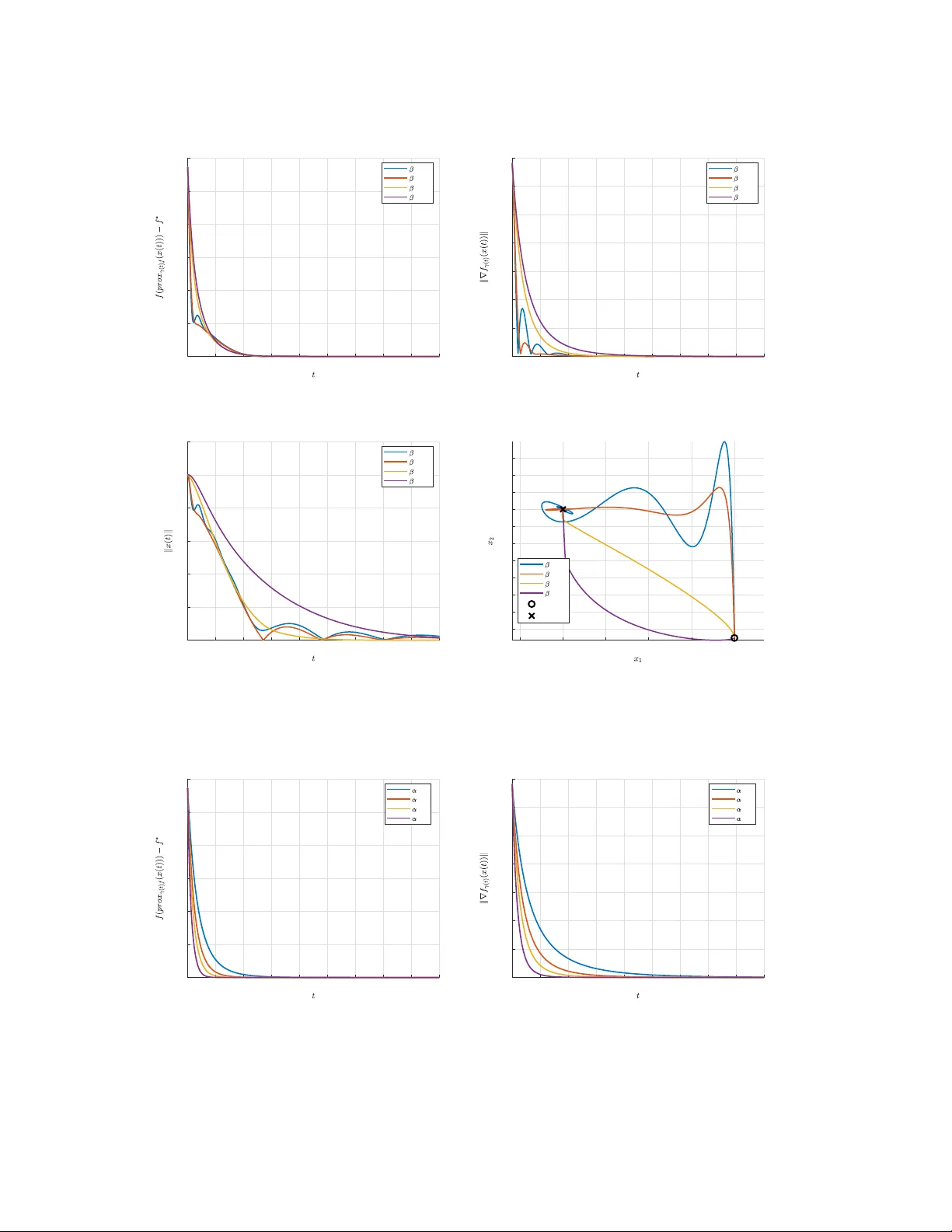
High-Res o lution Inertial Dynamics with T ime-Resc a led Gradients for Nonsmoo t h Con v ex Optimi z ation Manh Hung Le 1 Andrea Simonett o 2 A B S T R A C T . W e study no nsmooth con v ex min imization throu gh a con tinuous-time dynamica l system that can be seen as a high-reso lution ODE of Nestero v Accelera ted Gradient (N A G) adapted to the non smooth case. W e a pply a time-v arying M oreau en velope smoothing to a prop er con vex lo wer semicontin uous ob- jecti ve functi on and introdu ce a contro lled time-rescalin g of the gradie nt, cou pled with a Hessian-dri ven damping term, leadin g to our proposed inertial dynamic. W e prov ide a well-posed ness result for this dynamic al system, and construct a L yapuno v energy function captur ing the combined ef fects of inertia, damping , and smoothing. For an appropr iate scaling, the ener gy dissipat es and yields fast decay of the object ive function and gradient, stabilizati on of veloc ities, and w eak con ver genc e of trajectori es to mini- mizers under mild assumptions . Conceptu ally , the system is a nonsmooth high-r esolution model of Nes- tero v’ s method that clarifies ho w time-v arying smoothing and time rescaling jointly gover n acce leration and s tability . W e further ext end the fr amewor k to th e setting o f maximally mon otone operat ors, for which we propose and anal yze a corresp onding dynamical system and establ ish analogous con ver gence results. W e also present numerical experiments illustratin g the effec t of the main parameters and comparing the propo sed system with se veral be nchmark dynamics. AMS subject classificat ion: 34G20, 3 7N40, 49J 52, 65K10, 90C25. Ke y words and phrases : nonsmooth con vex opti mization; high-res olution dynamics; accelerati on meth- ods; Hessian- driv en damping ; time rescaling; Moreau en velope. 1 Introd uction 1.1 Pr oblem and mo tivation Let H be a real H ilbert space endo wed with the inner product h· , ·i and the associate d norm k · k . W e study the uncons trained con ve x (possib ly nonsmoot h) minimiza tion problem min x ∈H f ( x ) , (1.1) where f : H → R ∪ { + ∞} is prope r , con ve x, and lower semicontin uous, with nonempty sol ution set argmin H f 6 = ∅ . Such nonsmooth con ve x problems arise frequently in applicat ions (signal proc ess- ing, sta tistics, imaging, machine learning ) especi ally due to the presenc e of spars ity-inducin g or lo w- comple xity regulariz ers. First-order accelera ted metho ds, which achie ve faster con ver gence rates by in- corpor ating momentum, are particular ly v aluable for these prob lems. In discrete time, the prototypi cal 1 Unit ´ e de Math ´ ematiques Appliqu ´ ees, ENST A, Institut Polytechnique de Paris, 91120 Palaiseau, France. E-mail: manh- hung.le@ensta.fr 2 Unit ´ e de Math ´ ematiques Appliqu ´ ees, ENST A, Institut Polytechnique de Paris, 91120 Palaiseau, France. E-mail: an- drea.simonetto@ensta.fr 1 2 accele rated method is Nesterov’ s accelerated gradient (NA G) [18], which for smooth con ve x f attains an optimal O (1 /k 2 ) con ver gence rate in function val ue after k iteratio ns—significantl y faster than the O (1 /k ) rate of gradien t descen t or Polyak’ s hea vy-ball metho d [15, 20]. Our aim is to study an inertial (secon d-order) continuou s-time appro ach to solving (1.1), in the spirit of viewing optimization algorith ms throug h the lens of dynamical systems. Over the past decade, continuo us-time modeling of accelera ted methods has provi ded substant ial insights. In particu lar , low-r esolution ordinary dif ferential equations (ODEs) ha ve been deri ved that captur e the leadin g-order beha vior of momentum-base d algo rithms. A landmark result by S u, Boyd, and Candes [21] sho wed that N estero v’ s method can be seen as the discretiza tion of the second-o rder ODE ¨ x ( t ) + α t ˙ x ( t ) + ∇ f ( x ( t )) = 0 , with α = 3 . This van ishing-vis cosity ODE is a continuous- time analog of NA G and achie ves a con ver - gence rate f ( x ( t )) − min f = O (1 /t 2 ) for α ≥ 3 . Subsequent in vestiga tions [9, 10] establishe d tha t by using a slightly lar ger damping coefficien t (ef fectiv ely α > 3 in the abov e ODE ), one can ensure the weak con ver gence of x ( t ) to a minimizer and e ven impro ve the decay rate to o (1 /t 2 ) . This line of work for ged a firm link between N esterov’ s discrete method and L yapuno v-based con ver gence analysis in contin uous time. A complement ary perspe ctiv e was prov ided by W ibison o, Wi lson, and Jordan [23], who formulat ed a Bregman Lagran gian whose Euler–Lagra nge equation recov ers a family o f accele rated flows. Their va riational frame work expla ins m any accelera ted algorithms (includ ing NA G and its non-Eucli dean counte rparts) as dif ferent time-parameteriz ations of a single underl ying trajectory [23 ]. 1.2 High-resolution ODE models While the classical ODE ¨ x ( t ) + 3 t ˙ x ( t ) + ∇ f ( x ) = 0 replica tes NA G’ s O (1 /t 2 ) rate, it does so only at leading orde r and neglec ts certain subtle effects of dis- cretiza tion. Researchers hav e therefore sought higher -resolu tion dif ferential equation s that m ore faithful ly reflect the beha vior of the actual algori thms. A major work in this direc tion was the introd uction of a Hessian- driv en dampin g term by Attouch, Peypou quet, and Redon t [4]. They augmented the Neste rov ODE with an additio nal term in volv ing the Hessian ∇ 2 f , obtaining the flow ¨ x ( t ) + α t ˙ x ( t ) + β ∇ 2 f ( x ( t )) ˙ x ( t ) + ∇ f ( x ( t )) = 0 , with α ≥ 3 and β > 0 . This enrich ed model retains the O (1 /t 2 ) con ver gence rate in fun ction valu e, while dramatic ally reducing oscillatio ns and guarante eing a rapid decay of k∇ f ( x ( t )) k to 0 . The H essian - dri ven dampin g term can be interpr eted geometrica lly as a kind of curv ature-dep endent frictio n: since ∇ 2 f ( x ) ˙ x = d d t ∇ f ( x ( t )) , the extr a term acts like a deri vati ve of the gradie nt and helps to attenuate the oscilla tory ene rgy of the system. Building on this idea, A ttouch , Chbani, Fadili, and Riahi performed a detaile d study of a more general versio n of the above dynamics [5] as (DIN − A VD) α,β ,b ( t ) ¨ x ( t ) + α t ˙ x ( t ) + β ∇ 2 f ( x ( t )) ˙ x ( t ) + b ( t ) ∇ f ( x ( t )) = 0 . They demonst rated via a L yapuno v analysis that the continuo us traje ctory enjoys fast con ver gence of both functi on va lues and gradients. A partic ularly con venien t and theoretic ally rev ealing choice is b ( t ) = 1 + β /t . It is worth noticing that in [5] the authors performed a principled discretiza tion of their second - order dynamical system (DIN − A VD) α,β , 1+ β /t and obtaine d an algorithm named IGAHD; the numerical exp eriments carried out by the auth ors on ℓ 1 , ℓ 1 − ℓ 2 , T V , and nucle ar-no rm models sho wed that IGAHD 3 reduce d oscillatio ns and con ver ge at a faster rate tha n FIST A (the β = 0 case). In a subsequent wo rk, Attouch and Fadili [6] revisi ted the heav y-ball (Polyak) and Nestero v methods from a dynamical systems vie wpoint. They establishe d the so-called high-resol ution ODEs correspondi ng to both m ethods and re- vea led that both in v olve a Hessian-dri ven geomet ric damping term in contin uous time. S pecificall y , they obtain ed the followin g high-resol ution dynamic of N AG: ¨ x ( t ) + √ s ∇ 2 f ( x ( t )) ˙ x ( t ) + α t ˙ x ( t ) +  1 + α √ s 2 t  ∇ f ( x ( t )) = 0 . Their high-res olution appr oach rev eals two additional structures in the continuous -time limit of NA G: 1. A Hessian-dri ven damping term ∇ 2 f ( x ) ˙ x , and 2. A time-rescal ed grad ient of the form  1 + const t  ∇ f ( · ) . Interes tingly , we see that the app earance of Hessia n-dri ven damping can be rig orously understo od as a conseq uence of the high-r esolution ODE framewo rk. Further highlight ing the importanc e of high-re solution modeling, Shi, Du, S u, and Jordan [22] pointed out that the classi cal low-res olution ODEs (such as the Su–Boyd –Candes dynamic) do not actually disting uish between P olyak’ s momentum and Nestero v’ s method in certain regi mes. By deri ving high er-ord er dif fer - ential equation s and applying a symplectic (structu re-preservi ng) integr ator , Shi et al. were able to reco ver true accelerated algori thms in discre te time for smooth stro ngly con vex prob lems, whereas nai ve Euler discre tizations of the basic ODE often fail to do so [22]. A ll of these works undersco re that incorporat ing second -order informatio n (e.g. Hessian damping) and time-rescaled gradients into the continu ous model is crucial for capturin g and explainin g the distinct beha vior of accelerat ed optimizat ion m ethods. 1.3 T ime-rescaled dynamics Another fruitful directio n in conti nuous optimization dynamics is the use of time rescalin g to accelera te con ver gence. In standa rd gradient flow o r Nesterov ’ s flow , time is uniform; but one ca n intentional ly speed up the system’ s e volu tion by rescali ng time (or equi va lently , introduc ing time-va rying coef ficients in the ODE). For example, consider modifying the Nesterov ODE to ¨ x ( t ) + α t ˙ x ( t ) + b ( t ) ∇ f ( x ( t )) = 0 , where b is an increasi ng functio n. As sho wn by Attouch, Chbani, and Riahi [7], the fact or b ( t ) ef fectiv ely accele rates the drivin g gradient force and can yield improv ed decay rates of order O  1 t 2 b ( t )  . 1.4 Mor eau en velope smoothing for nonsmooth problems The d iscussion so far has assumed f is smooth (at least C 1 with Lipschitz gradi ent). Howe ver , our ultimate interes t is the nonsmooth case, where f may not be dif ferentiable . A stand ard approa ch to handle a nonsmoo th con ve x f is to introdu ce its Moreau en velope . For γ > 0 , the Moreau en velope of a proper , con ve x, and lo wer semicontinuo us function f : H → R ∪ { + ∞} with parameter γ is defined by f γ ( x ) := min y ∈H n f ( y ) + 1 2 γ k x − y k 2 o . The unique minimizer in the definition is gi ven by the proximal map pro x γ f ( x ) := arg min y ∈H n f ( y ) + 1 2 γ k x − y k 2 o . The Moreau en velo pe satisfies the followin g classical proper ties: 4 1. f γ is con ve x and continuous ly diffe rentiable ev en if f is nonsmooth ; 2. T he gradie nt is Lipschitz with ∇ f γ ( x ) = 1 γ  x − pro x γ f ( x )  and k∇ f γ ( x ) − ∇ f γ ( y ) k ≤ 1 γ k x − y k ; 3. T he en velope preserv es the set of minimizers, i.e., arg min f γ = arg m in f . Hence, f γ pro vides a smooth approx imation of f that retains the same minimizers and has a controlled gradie nt Lipschi tz constant 1 /γ . This smoothing techniq ue has been le veraged in continuous dynamics by Attouch and Cabot [3], who w ere among the fi rst to analyze an inertial Moreau-en velop e flo w for nonsmoo th optimization . They consider ed the ODE ¨ x ( t ) + α t ˙ x ( t ) + ∇ f λ ( t ) ( x ( t )) = 0 , where λ ( t ) is a smoothin g parameter that may slo wly va ry with time. They prov ed that by approp riately choos ing λ ( t ) , the trajec tory x ( t ) enjo ys ac celerated con ver gence in terms of the smoothe d obj ectiv e: f λ ( t ) ( x ( t )) − f ∗ = o (1 /t 2 ) , along w ith k ˙ x ( t ) k = o (1 /t ) and weak con ver gence of x ( t ) to a minimizer . Furthermor e, these con ver gence rates for the en velope tran slate back to the orig inal objecti ve via a prox - imal shado w argu ment, meaning the true function va lues f ( x ( t )) also approach the optimum. More re- cently , Attouch and Laszl ´ o [11] incorporat ed Hessian-dri ven damping into such an en velope -based inertial dynamic . They sho wed that adding the β d d t ∇ f λ ( x ( t )) term yields similar con ver gence properties as in the smooth case (fast decay of the en velop e’ s gradient norm, etc.) Concurren tly , other researchers hav e exp lored contin uous-time methods that combine en velop e smooth ing with time rescaling or other regul ar- ization techni ques. For exampl e, B ot ¸ and Karapetyants [13] proposed a fast inertia l flow for nonsmoo th con ve x problems that employ s an ex plicit time scaling together with the Moreau en velope smoothing to achie ve acceler ated con ver gence. In a follo w-up work, Karapety ants [17] studied a related continuo us-time approa ch using Tikh onov (ridge) regulari zation of the objecti ve, and provided con ver gence gua rantees for the resulting tra jectories. Other rel ev ant litera ture is captured by the works of [1, 2, 11, 12, 14, 24]. In genera l, these works confirm that the po werful accelerat ion principles kno wn for smooth dynamics (mo- mentum, time rescalin g, etc.) can be successfully transferre d to the nonsmooth setting by working with reg ularized/smoo thed surrogates of f . 1.5 Our dynamics: a nonsmooth high-resolution appr oach with time-rescaled gradients W e buil d on this ric h literatu re by formulating a ne w high- resolution inertial dynamic tailo red to nons- mooth con vex m inimizati on. Our dynamical system employs both the high-res olution framew ork [6 ] and the time-rescaled gradients (as in Attouch–Chban i–Riahi [7]), applied in conjuncti on with a time-v arying Moreau en velope smoothing of f . ¨ x ( t ) + α t ˙ x ( t ) + β d d t h δ ( t ) ∇ f γ ( t ) ( x ( t )) i +  1 + β t  δ ( t ) ∇ f γ ( t ) ( x ( t )) = 0 . ( NS-HR ) α,β (1.2) Here the parameters hav e the follo wing roles: • α > 0 : contro ls the van ishing viscous damping coefficien t α/t ; 5 • β > 0 : weights the Hessian-dri ven damping contrib ution; • γ ( t ) > 0 : specifies the time-va rying smoothing parameter in the M oreau en velop e f γ ( t ) ; • δ ( t ) > 0 : gov erns the time-resc aling of the gradient. Let us stress that the en velo pe yields C 1 smoothn ess with L ipschit z gradient, preserv es arg min f , and lets us encode H essian- driv en damp ing through the time deri va tiv e of ∇ f γ ( t ) without computing Hes- sians. It is worth noti cing that our dynamic s can be seen as a nonsmooth, time-rescal ed extens ion of the (DIN − A VD) α,β , 1+ β /t studie d in the smooth case by Attouch et al. [5 ]. W e will also extend ( NS-HR ) α,β to deal with the problem of fi nding zeros of maximally m onoton e opera- tors. Specifically , we are interested in: Find x ∈ H : 0 ∈ A ( x ) , where A : H → 2 H is a maximally monotone operator . Analogo usly to the case of nonsmooth optimization , we propose the follo wing dynamic: ¨ x ( t ) + α t ˙ x ( t ) + β d d t h δ ( t ) A γ ( t ) ( x ( t )) i +  1 + β t  δ ( t ) A γ ( t ) ( x ( t )) = 0 , ( HR-MMD ) α,β where A γ ( t ) is the Y osi da approx imation of A with constan t γ ( t ) . Partic ularizations and links to existing d ynamics. T he propose d dynamical system (NS - HR) α,β can be viewed as a unifying template that recov ers se ver al cla ssical conti nuous-time models for accelerated optimiza tion as soon as the parameters ( α, β , δ , γ ) are special ized. Low-r esolution and time-resc aled limits. Setting β = 0 remov es the high-reso lution term and yield s a lo w-resolution inertia l en velop e flo w [13] ¨ x ( t ) + α t ˙ x ( t ) + δ ( t ) ∇ f γ ( t ) ( x ( t )) = 0 . When δ ( t ) ≡ 1 , this recov ers the nonsmooth inertial Moreau-en velop e dyna mics studied in [3] (with time- depen dent smoothing). When γ ( t ) is negle cted, one obtain s a time-resc aled N esterov-ty pe flow of the form ¨ x + α t ˙ x + b ( t ) ∇ f ( x ) = 0 [7]. In part icular , taking δ ( t ) ≡ 1 and β = 0 reco vers the Su–Boyd –Cand ` es ODE ¨ x + α t ˙ x + ∇ f ( x ) = 0 in the smooth setting [21]. High-res olution/Hessi an-d rive n damping limits. When β > 0 , the term d dt ( δ ( t ) ∇ f γ ( t ) ( x ( t ))) introdu ces a Hessian-d riv en damping ef fect w ithout ex plicit Hessian computation s, since for smooth f one has d dt ( ∇ f ( x ( t ))) = ∇ 2 f ( x ( t )) ˙ x ( t ) . If f is smooth, δ ( t ) ≡ 1 , and γ ( t ) is neglecte d, (NS - HR) α,β reduce s to the high-resolu tion inertial system (DIN - A VD) α,β , 1+ β/t studie d in [5], which underlies the IGA H D discre tization (in the same paper). Over all, (NS - HR) α,β pro vides a common en velop e-based extensio n of lo w-resolution Nestero v flows, time-rescale d inertial dynamics, and high-resolu tion Hessian-d amped models. Contrib u tion of the paper 1. N onsmooth high-re solution dynamic with time-r escaled gradients. W e propose and stud y the dynamic al system ( NS-HR ) α,β , which can be vie wed as a high-resol ution continu ous-time model tailore d for nons mooth con ve x optimization. This model incorporat es sev eral ke y mechanisms si- multaneo usly: a vanis hing visco us damping term that gov erns long-term sta bilization, a Hessian- dri ven damping component inher ited from the high -resolution ODE perspect ive , and a gradien t 6 T able 1: Particulari zations of (NS - HR) α,β highli ghted in the discuss ion. Paramet er choice Resulting d ynamics Refer ence β = 0 (general δ, γ ) ¨ x ( t ) + α t ˙ x ( t ) + δ ( t ) ∇ f γ ( t ) ( x ( t )) = 0 (lo w- resolu tion inertial en velope flow) [13] β = 0 , δ ( t ) ≡ 1 ¨ x ( t ) + α t ˙ x ( t ) + ∇ f γ ( t ) ( x ( t )) = 0 (nonsmoot h in- ertial Moreau-en velope dynamics with smoothin g) [3] β = 0 , γ ( t ) neglecte d , δ ( t ) = b ( t ) ¨ x ( t ) + α t ˙ x ( t ) + b ( t ) ∇ f ( x ( t )) = 0 (time-re scaled Nestero v-type flow) [7] β = 0 , δ ( t ) ≡ 1 , γ ( t ) neglecte d ¨ x ( t ) + α t ˙ x ( t ) + ∇ f ( x ( t )) = 0 (Su–Boyd–Cand ` es lo w-resolution ODE) [21] β > 0 , δ ( t ) ≡ 1 , γ ( t ) neglecte d , f smooth (DIN - A V D ) α,β , 1+ β /t (high- resolution inertia l system / Hessian-d riv en damping limit) [5] term whose magnitude is appropr iately resca led in time. W e furthe r show that ( NS-HR ) α,β ad- mits an equiv alent first-order formulati on, which plays a crucial role in potential discreti zations. In additi on, we establish a rigorou s well-posedne ss theory for the syst em by pro ving global exis tence and unique ness of solutions under natural assumptio ns on the data. 2. L yapunov framewor k and asymptotics. W e constru ct a L yapunov function specifical ly adapted to ( NS-HR ) α,β . T his function al allo ws us to deri ve a detailed quantitati ve description of the asymptotic beha vior of the trajectories . In particular , we obtain arbitraril y fast decay rates for both objecti ve functi on valu es and gradient norms, demons trating that the system can achi ev e accelera ted con ver - gence in a precise sense. Furthermore, we show stabiliz ation of the velocit y field and prov e the w eak con ver gence of trajector ies to ward minimizers of the underlyin g con ve x functio n, thereby providin g a complete qualitat iv e pictur e of the dynamics. 3. E xtension to maximally monotone operator s. W e propos e the dynamica l system ( HR -MM D ) α,β and ext end the analys is dev eloped in the con vex optimiz ation setting to the broader and more abstra ct frame work of finding zeros of maximall y mono tone ope rators. In this exte nsion, we demonstrat e that the funda mental structural results, includ ing well-pos edness, L yapun ov decay estimates, and con ver gence properties, carry over under appropriate assumpti ons. 4. N umerical experiments and a p r oximal discreti zation perspectiv e. W e complement the theore ti- cal analysis with a series of numerical experimen ts illustratin g the influence of the parameters β and α , as well as compariso ns w ith sev eral benchmark dynamics from the literature. These exper iments highli ght the damping effec t of the Hessian-dr iv en ter m, confirm our theoretical results, and sho w the fa vo rable beha vior of the propos ed system relati ve to competing approach es. In addit ion, we de- ri ve a natural second -order time disc retization of (NS - HR) α,β and sho w that the resu lting implicit scheme can be resolv ed by a single proxima l step, thereby provid ing an algorithmic coun terpart of the continu ous model. 1.6 Paper o utline The remainde r of the paper is org anized as follo ws. Section 2 deri ves an equiv alent first-order reformu- lation of (NS - HR) α,β , and establish es global existen ce and uniquen ess of solution trajectories. Section 3 de velops the main L yapuno v frame work and provides the asymptotic analy sis of the system, includi ng fast decay rates for the Moreau -en velo pe objecti ve residu al and gradient norm, stabilization of velocitie s, 7 and weak con ver gence of trajectories under suitable assumpti ons on the time-depen dent parameters . Sec- tion 4 exten ds the analysis to the setting of maximally monoto ne operators through the corres ponding high-r esolution Y osida-r egulariz ed dynamic. Sectio n 5 discuss es the relationshi p between the two analy- ses and highligh ts similarities and dif ferences between the optimiza tion and m onoto ne-inclusio n settings. Section 6 discusses a natural discretizat ion of (NS - HR) α,β , sho wing that the resulting implicit scheme can be resolved through a single proximal step. Section 7 is dev oted to numerical experimen ts: we in vestiga te the influence of the parameters β and α , and compare the proposed system w ith sev eral referenc e dynam- ics from the literature. F inally , Section 8 concludes the paper and outlines sev eral perspecti ves for future work. 2 W ellposedness of ( NS-HR ) α,β 2.1 First-order ref o rmulatio n of ( NS-HR ) α,β W e start with a fi rst-ord er reformula tion of ( NS-HR ) α,β , w hich we will lev erage in the subsequent proofs. Theor em 2.1 Suppose δ : [ t 0 , + ∞ ) → (0 , + ∞ ) and γ : [ t 0 , + ∞ ) → (0 , + ∞ ) ar e continuo usly dif fer en- tiable functio ns. Let ( x 0 , v 0 , y 0 ) ∈ H 3 satisfy ing v 0 = − β δ ( t 0 ) ∇ f γ ( t 0 ) ( x 0 ) −  α − 1 t 0 − 1 β  x 0 − 1 β y 0 . (2.1) Then, the following ar e equivalent (i) x is a solution to ( NS-HR ) α,β with x ( t 0 ) = x 0 , and ˙ x ( t 0 ) = v 0 . (ii) Ther e exis ts y suc h that ( x, y ) satisfie s ˙ x ( t ) + β δ ( t ) ∇ f γ ( t ) ( x ( t )) +  α − 1 t − 1 β  x ( t ) + 1 β y ( t ) = 0 , (2.2) ˙ y ( t ) −  1 β − α − 2 t  x ( t ) +  1 t + 1 β  y ( t ) = 0 , (2.3) with ( x ( t 0 ) , y ( t 0 )) = ( x 0 , y 0 ) . Pro of. (ii) ⇒ (i). Let us dif ferentiate (2.2): ¨ x ( t ) + β d d t h δ ( t ) ∇ f γ ( t ) ( x ( t )) i +  α − 1 t − 1 β  ˙ x ( t ) − α − 1 t 2 x ( t ) + 1 β ˙ y ( t ) = 0 . This implies ¨ x ( t ) + α t ˙ x ( t ) + β d d t h δ ( t ) ∇ f γ ( t ) ( x ( t )) i −  1 t + 1 β  ˙ x ( t ) − α − 1 t 2 x ( t ) + 1 β ˙ y ( t ) = 0 . (2.4 ) From (2.4), to conclude that x has to satisfy ( NS-HR ) α,β , it suf fices to prov e that −  1 t + 1 β  ˙ x ( t ) − α − 1 t 2 x ( t ) + 1 β ˙ y ( t ) =  1 + β t  δ ( t ) ∇ f γ ( t ) ( x ( t )) . 8 Indeed , from the first-order formulation w e yield −  1 t + 1 β  ˙ x ( t ) − α − 1 t 2 x ( t ) + 1 β ˙ y ( t ) = −  1 t + 1 β h − β δ ( t ) ∇ f γ ( t ) ( x ( t )) −  α − 1 t − 1 β  x ( t ) − 1 β y ( t ) i − α − 1 t 2 x ( t ) + 1 β h 1 β − α − 2 t  x ( t ) −  1 t + 1 β  y ( t ) i =  1 + β t  δ ( t ) ∇ f γ ( t ) ( x ( t )) + h 1 t + 1 β  α − 1 t − 1 β  − α − 1 t 2 + 1 β  1 β − α − 2 t i x ( t ) + h 1 t + 1 β  1 β  − 1 β  1 t + 1 β i y ( t ) . The proof for this implication is thereby completed by noticin g     1 t + 1 β  α − 1 t − 1 β  − α − 1 t 2 + 1 β  1 β − α − 2 t  = 0 ,  1 t + 1 β  1 β  − 1 β  1 t + 1 β  = 0 , and that the initial condition is automaticall y satisfied by the requirement on v 0 exp ressed in Eq. (2.1). (i) ⇒ (ii). D efine y : [ t 0 , + ∞ ) − → H according to the requirement on v 0 exp ressed in E q. (2.1) as well as the equatio n ˙ x ( t ) + β δ ( t ) ∇ f γ ( t ) ( x ( t )) +  α − 1 t − 1 β  x ( t ) + 1 β y ( t ) = 0 . (2.5) As pre viously seen, the dif ferentiatio n of this equation with respec t to t gi ves the second-or der dynamic ¨ x ( t ) + α t ˙ x ( t ) + β d d t h δ ( t ) ∇ f γ ( t ) ( x ( t )) i −  1 t + 1 β  ˙ x ( t ) − α − 1 t 2 x ( t ) + 1 β ˙ y ( t ) = 0 . (2.6 ) From the definition of x and y , namely ( NS -H R ) α,β and (2.5) we ha ve    ¨ x ( t ) + α t ˙ x ( t ) + β d d t h δ ( t ) ∇ f γ ( t ) ( x ( t )) i = −  1 + β t  δ ( t ) ∇ f γ ( t ) ( x ( t )) , −  1 t + 1 β  ˙ x ( t ) =  1 + β t  δ ( t ) ∇ f γ ( t ) ( x ( t )) +  1 t + 1 β  α − 1 t − 1 β  x ( t ) + 1 β  1 t + 1 β  y ( t ) . Plugging these identitie s in (2.6) gi ves −  1 + β t  δ ( t ) ∇ f γ ( t ) ( x ( t )) +  1 + β t  δ ( t ) ∇ f γ ( t ) ( x ( t )) +  1 t + 1 β  α − 1 t − 1 β  x ( t ) + 1 β  1 t + 1 β  y ( t ) − α − 1 t 2 x ( t ) + 1 β ˙ y ( t ) = 0 . Simplification yields 1 β  α − 2 t − 1 β  x ( t ) + 1 β  1 t + 1 β  y ( t ) + 1 β ˙ y ( t ) = 0 . Multiply ing this equation by β giv es (2.3), hence completing the proof.  9 2.2 Existence and uniqueness of a solution trajectory of ( N S-HR ) α,β T o establish the existen ce an d uniquen ess of a soluti on to ( N S -HR ) α,β , we make use of its first-order reformul ation. Set z ( t ) = ( x ( t ) , y ( t )) , and F : [ t 0 , + ∞ ) × H 2 → H 2 defined by F ( t, ( x, y )) = h − β δ ( t ) ∇ f γ ( t ) ( x ) −  α − 1 t − 1 β  x − 1 β y ,  1 β − α − 2 t  x −  1 t + 1 β  y i . (2.7) ( NS-HR ) α,β can no w be written equi vale ntly as ˙ z ( t ) = F ( t, z ( t )) . W e now will rely on the following result [16, Proposition 6.2.1]. Theor em 2.2 [16, Pr oposit ion 6.2.1] Let X be a Banach space, s 0 > 0 , and g : [ s 0 , + ∞ ) × X − → X . Suppo se that g satisfi es the following pr operties: (i) ∀ x ∈ X , g ( · , x ) ∈ L 1 loc ([ s 0 , + ∞ ) , X ) . (ii) F or a.e. t ∈ [ s 0 , + ∞ ) , g ( t, · ) : X − → X is continu ous and satisfies ∀ x, y ∈ X , k g ( t, x ) − g ( t, y ) k ≤ K ( t, k x k + k y k ) k x − y k , wher e K ( · , r ) ∈ L 1 loc ([ s 0 , + ∞ )) ∀ r ≥ 0 . (iii) F or a.e. t ∈ [ s 0 , + ∞ ) , g ( t, · ) : X − → X satisfies k g ( t, x ) k ≤ P ( t )(1 + k x k ) ∀ x ∈ X , wher e P ∈ L 1 loc ([ s 0 , + ∞ )) . Then, for ever y u 0 ∈ X , ther e exists a unique function u ∈ W 1 , 1 loc ([ s 0 , + ∞ ) , X ) , i.e., u is local ly absolutely contin uous on [ s 0 , + ∞ ) , such that ( ˙ u ( t ) = g ( t, u ( t )) for a.e. t ∈ [ s 0 , + ∞ ) , u ( s 0 ) = u 0 . W e are now ready to present and prov e the exist ence and uniquen ess result for ( NS-HR ) α,β . Theor em 2.3 Let t 0 > 0 be an arbitr ary starting time. Suppo se δ : [ t 0 , + ∞ ) → (0 , + ∞ ) and γ : [ t 0 , + ∞ ) → (0 , + ∞ ) ar e continuous ly diffe ren tiable funct ions. Then given any pair ( x 0 , v 0 ) ∈ H 2 , ther e e xists a unique solution trajecto ry x ∈ W 1 , 1 loc ([ t 0 , + ∞ )) that satisfi es ( NS-HR ) α,β almost everywher e on [ t 0 , + ∞ ) with the intial condition ( x ( t 0 ) , ˙ x ( t 0 )) = ( x 0 , v 0 ) . Pro of. One can see that for all ( x, y ) ∈ H 2 , F ( · , x, y ) defined in Eq. (2.7) is continuo us on [ t 0 , + ∞ ) , and therefo re F ( · , x, y ) ∈ L 1 loc ([ t 0 , + ∞ ) , H 2 ) . It remains to verify that F satisfies the last two requiremen ts of T heorem 2.2. V erify that F satisfies the r equ irement (ii) of Theorem 2.2 Giv en ( x, y ) ∈ H 2 and ( u, v ) ∈ H 2 , w e consid er the diff erence k F ( t, x, y ) − F ( t, u, v ) k = h    β δ ( t )  ∇ f γ ( t ) ( u ) − ∇ f γ ( t ) ( x )  +  α − 1 t − 1 β  ( u − x ) + 1 β ( v − y )    2 +     1 β − α − 2 t  ( x − u ) +  1 t + 1 β  ( v − y )    2 i 1 / 2 10 This equality , combined with the 1 γ ( t ) − Lipschitz continu ity of ∇ f γ ( t ) and the triangle inequality , implies k F ( t, x, y ) − F ( t, u, v ) k ≤ β δ ( t ) γ ( t ) k u − x k +    α − 1 t − 1 β    k u − x k + 1 β k v − y k +    1 β − α − 2 t    k x − u k +    1 t + 1 β    k v − y k ≤ a ( t ) k u − x k + b ( t ) k v − y k , where we hav e con veni ently set a ( t ) = β δ ( t ) γ ( t ) +    α − 1 t − 1 β    +    1 β − α − 2 t    , b ( t ) = 1 β +    1 t + 1 β    . W e further obtain k F ( t, x, y ) − F ( t, u, v ) k ≤ K ( t ) k ( x, y ) − ( u, v ) k , where K ( t ) :=  a ( t ) 2 + b ( t ) 2  1 / 2 . As such, since a ∈ L 1 loc ([ t 0 , + ∞ )) and b ∈ L 1 loc ([ t 0 , + ∞ )) , then K ∈ L 1 loc ([ t 0 , + ∞ )) . V erify that F satisfies the r equ irement (iii) of Theore m 2.2 Consider any minimizer of f , which we indicate as x ∗ . From the definition of F , we ha ve k F ( t, x, y ) k ≤    − β δ ( t ) ∇ f γ ( t ) ( x ) −  α − 1 t − 1 β  x − 1 β y    +     1 β − α − 2 t  x −  1 t + 1 β  y    ≤ β δ ( t ) γ ( t ) k x − x ∗ k +     α − 1 t − 1 β    +    1 β − α − 2 t     k x k +  1 β +    1 t + 1 β     k y k ≤ β δ ( t ) γ ( t ) k x ∗ k + a ( t ) k x k + b ( t ) k y k ≤ β δ ( t ) γ ( t ) k x ∗ k + K ( t ) k ( x, y ) k . Set P ( t ) = max  β δ ( t ) γ ( t ) k x ∗ k , K ( t )  . W e obtain k F ( t, x, y ) k ≤ P ( t )(1 + k ( x, y ) k ) . As such, P ∈ L 1 loc ([ t 0 , + ∞ )) . The proof is thereby completed.  3 Con vergence properties of ( NS-HR ) α,β Before going into the con ver gence analysi s of ( NS -H R ) α,β , we need to make the followin g assumption on the va lues of the coef ficients. Assumption 3.1 Let α > 3 , and β > 0 . Let δ , γ : [ t 0 , + ∞ ) → (0 , + ∞ ) be C 1 functi ons satisfying: (i) lim inf t → + ∞ ˙ γ ( t ) tδ ( t ) > 0 . 11 (ii) tδ ( t ) γ ( t ) = O (1 /t ) . (iii) ˙ γ ( t ) γ ( t ) = O (1 /t ) . (iv) T her e exis ts 0 < ζ ≤ α − 3 such that for all lar ge t , 0 ≤ t ˙ δ ( t ) δ ( t ) ≤ α − 3 − ζ . Remark 3.1 Assumption 3.1 is m ild. F or instance , it is verified with the polynomial s δ ( t ) = t p , γ ( t ) = ct p +2 ( t ≥ t 0 > 0) , wher e c > 0 and p ∈ [0 , α − 3) . Indeed : (i) Since ˙ γ ( t ) = c ( p + 2) t p +1 , ˙ γ ( t ) tδ ( t ) = c ( p + 2) t p +1 t · t p = c ( p + 2) , and ther efor e lim inf t → + ∞ ˙ γ ( t ) tδ ( t ) = c ( p + 2) > 0 . (ii) tδ ( t ) γ ( t ) = t · t p ct p +2 = 1 ct = O  1 t  . (iii) ˙ γ ( t ) γ ( t ) = c ( p + 2) t p +1 ct p +2 = p + 2 t = O  1 t  . (iv) Since ˙ δ ( t ) = pt p − 1 , t ˙ δ ( t ) δ ( t ) = t · pt p − 1 t p = p. Choose , for instance , ζ := α − 3 − p 2 ∈ (0 , α − 3) , so that 0 ≤ p ≤ α − 3 − ζ for all lar ge t . Since ar gmin H f 6 = ∅ , we fi x some x ∗ ∈ ar gmin H f . For the con ver gence analysis of ( NS-H R ) α,β , we emplo y the L yapuno v functio n V := V 1 + V σ ,η , w here V 1 ( t ) = a ( t )  f γ ( t ) ( x ( t )) − f ∗  , (3.1) V σ ,η ( t ) = 1 2    σ ( x ( t ) − x ∗ ) + t ˙ x ( t ) + β tδ ( t ) ∇ f γ ( t ) ( x ( t ))    2 + η k x ( t ) − x ∗ k 2 , (3.2) with 0 < σ < α − 1 being chosen later , and the coeffici ents a and η being defined as follows a ( t ) = h t − β ( σ + 1 − α ) i tδ ( t ) , η = σ ( α − σ − 1) 2 . W e will need the followin g technical lemma for the con ver gence analysis. 12 Lemma 3.1 Suppose that δ, γ : [ t 0 , + ∞ ) → (0 , + ∞ ) , and x : [ t 0 , + ∞ ) → H ar e of class C 1 . Suppose that f : H → R ∪ { + ∞} is pr oper , con vex, and lower semiconti nuous. T hen, w e have    d d t [ δ ( t ) ∇ f γ ( t ) ( x ( t ))]    ≤ δ ( t ) γ ( t ) k ˙ x ( t ) k + h 2 δ ( t ) | ˙ γ ( t ) | γ ( t ) 2 + | ˙ δ ( t ) | γ ( t ) i k x ( t ) − x ∗ k . Pro of. The lemma is a direct corolla ry of the more general Lemma 4.2, which w e will prov e later .  W e are now in the positio n to present the con ver gence properties of ( NS-HR ) α,β . Theor em 3.1 Under the standing A ssumption 3.1, and for any solut ion trajector y x : [ t 0 , + ∞ ) → H to ( NS-HR ) α,β , we have (i) f γ ( t ) ( x ( t )) − f ∗ = o  1 t 2 δ ( t )  . (ii) k∇ f γ ( t ) ( x ( t )) k = o  1 t 2 δ ( t )  . (iii) k ˙ x ( t ) k = o ( 1 t ) . (iv) Z + ∞ t 0 t k ˙ x ( t ) k 2 d t < + ∞ . (v) Z + ∞ t 0 t 3 δ ( t ) 2 k∇ f γ ( t ) ( x ( t )) k 2 d t < + ∞ . (vi) if in addition lim inf t → + ∞ t 2 δ ( t ) γ ( t ) > 0 , then x ( t ) con ver ges weakly as t → + ∞ , and its limit belongs to ar gmin H f . Pro of. T he proof proceeds by defining a suitab le L yapunov function and computin g its deriv ati ve. By using the standing assumptio ns, we will then be able to bound key terms and prove items (iv) and (v) . W e then use these bounds to prov e the rates for the ve locity (iii) , the gradient (ii) , and the functional gap (i) . W e then conclude by lev eraging Opial’ s lemma to prove weak con ver gence of the trajecto ry (vi) . As announced , we consider the follo wing L yapun ov function V ( t ) := V 1 ( t ) + V σ ,η ( t ) as defined in E qua- tions (3.1)-(3.2). Along the trajectory x ( t ) , the L yapunov function is nonne gati ve for sufficien tly large t . W e compute the deriv ativ e of V 1 ˙ V 1 ( t ) = ˙ a ( t )  f γ ( t ) ( x ( t )) − f ∗  + a ( t ) d d t f γ ( t ) ( x ( t )) . By the chain rule d d t f γ ( t ) ( x ( t )) = ˙ γ ( t ) d d γ f γ ( x ( t ))     γ = γ ( t ) + D ˙ x ( t ) , ∇ f γ ( t ) ( x ( t )) E . W e now recall a result concerning the deri vati ve of the Moreau en velope f γ with respect to γ [3] d d γ f γ ( x ) = − 1 2 k∇ f γ ( x ) k 2 ∀ x ∈ H . 13 As a result, ˙ V 1 ( t ) = ˙ a ( t )  f γ ( t ) ( x ( t )) − f ∗  − ˙ γ ( t ) a ( t ) 2 k∇ f γ ( t ) ( x ( t )) k 2 + a ( t ) D ˙ x ( t ) , ∇ f γ ( t ) ( x ( t )) . E (3.3) W e now turn to computing the deri vat ive V σ ,η . W e hav e ˙ V σ ,η ( t ) = D σ ( x ( t ) − x ∗ ) + t ˙ x ( t ) + β tδ ( t ) ∇ f γ ( t ) ( x ( t )) , ( σ + 1) ˙ x ( t ) + t ¨ x ( t ) + β d d t h tδ ( t ) ∇ f γ ( t ) ( x ( t )) iE + 2 η h x ( t ) − x ∗ , ˙ x ( t ) i . (3.4) From the expres sion of ( NS-HR ) α,β , w e can expre ss the term t ¨ x ( t ) as t ¨ x ( t ) = − α ˙ x ( t ) − β t d d t h δ ( t ) ∇ f γ ( t ) ( x ( t )) i − ( t + β ) δ ( t ) ∇ f γ ( t ) ( x ( t )) , and by substitut ing this equi v alence into (3.4) and simplifying, we obtain ˙ V σ ,η ( t ) = D σ ( x ( t ) − x ∗ ) + t ˙ x ( t ) + β tδ ( t ) ∇ f γ ( t ) ( x ( t )) , ( σ + 1 − α ) ˙ x ( t ) − tδ ( t ) ∇ f γ ( t ) ( x ( t )) E + 2 η h x ( t ) − x ∗ , ˙ x ( t ) i . Further algebraic manipulat ions yield ˙ V σ ,η ( t ) = h σ ( σ + 1 − α ) + 2 η i h x ( t ) − x ∗ , ˙ x ( t ) i + t ( σ + 1 − α ) k ˙ x ( t ) k 2 + h β ( σ + 1 − α ) − t i tδ ( t ) D ∇ f γ ( t ) ( x ( t )) , ˙ x ( t ) E − σ tδ ( t ) D ∇ f γ ( t ) ( x ( t )) , x ( t ) − x ∗ E − β t 2 δ ( t ) 2    ∇ f γ ( t ) ( x ( t ))    2 . From the con vexit y of f γ ( t ) , we kno w that D ∇ f γ ( t ) ( x ( t )) , x ( t ) − x ∗ E ≥ f γ ( t ) ( x ( t )) − f ∗ . As such, we can upper bound ˙ V σ ,η ( t ) as ˙ V σ ,η ( t ) ≤ h σ ( σ + 1 − α ) + 2 η i h x ( t ) − x ∗ , ˙ x ( t ) i + t ( σ + 1 − α ) k ˙ x ( t ) k 2 + h β ( σ + 1 − α ) − t i tδ ( t ) D ∇ f γ ( t ) ( x ( t )) , ˙ x ( t ) E − σ tδ ( t )  f γ ( t ) ( x ( t )) − f ∗  − β t 2 δ ( t ) 2    ∇ f γ ( t ) ( x ( t ))    2 . (3.5) By adding the expres sions (3.3) with (3.5), w e arri ve at the bound, ˙ V ( t ) ≤  ˙ a ( t ) − σ tδ ( t )  f γ ( t ) ( x ( t )) − f ∗  + h σ ( σ + 1 − α ) + 2 η i h x ( t ) − x ∗ , ˙ x ( t ) i + t ( σ + 1 − α ) k ˙ x ( t ) k 2 −  β t 2 δ ( t ) 2 + ˙ γ ( t ) a ( t ) 2  k∇ f γ ( t ) ( x ( t )) k 2 + n a ( t ) + h β ( σ + 1 − α ) − t i tδ ( t ) oD ∇ f γ ( t ) ( x ( t )) , ˙ x ( t ) E . Substitu ting now the definition of a ( t ) and η , ˙ V ( t ) ≤  ˙ a ( t ) − σ tδ ( t )  f γ ( t ) ( x ( t )) − f ∗  + t ( σ + 1 − α ) k ˙ x ( t ) k 2 −  β t 2 δ ( t ) 2 + ˙ γ ( t ) a ( t ) 2  k∇ f γ ( t ) ( x ( t )) k 2 . 14 From Assumption 3.1 (iv) , one can easily sho w that for a suitably chosen σ ∈ (0 , α − 1) , we hav e ˙ a ( t ) − σ tδ ( t ) ≤ 0 for sufficien tly larg e t . Indeed, a ( t ) =  t − β ( σ + 1 − α )  t δ ( t ) =  t 2 − β ( σ + 1 − α ) t  δ ( t ) . Dif ferentiating , we obtain ˙ a ( t ) =  2 t − β ( σ + 1 − α )  δ ( t ) +  t 2 − β ( σ + 1 − α ) t  ˙ δ ( t ) . Hence ˙ a ( t ) − σ tδ ( t ) =  (2 − σ ) t − β ( σ + 1 − α )  δ ( t ) +  t 2 − β ( σ + 1 − α ) t  ˙ δ ( t ) . Div iding by tδ ( t ) , we get ˙ a ( t ) − σ tδ ( t ) tδ ( t ) = (2 − σ ) − β ( σ + 1 − α ) t +  t − β ( σ + 1 − α )  ˙ δ ( t ) δ ( t ) . Equi vale ntly , ˙ a ( t ) − σ tδ ( t ) tδ ( t ) = (2 − σ ) − β ( σ + 1 − α ) t +  1 − β ( σ + 1 − α ) t  t ˙ δ ( t ) δ ( t ) . By Assumption 3.1 (iv) , there exists 0 < ζ ≤ α − 3 such that for all sufficien tly large t , 0 ≤ t ˙ δ ( t ) δ ( t ) ≤ α − 3 − ζ . Therefore , for all sufficie ntly large t , ˙ a ( t ) − σ tδ ( t ) tδ ( t ) ≤ (2 − σ ) − β ( σ + 1 − α ) t +  1 − β ( σ + 1 − α ) t  ( α − 3 − ζ ) . Letting t → + ∞ , the right-han d side tends to (2 − σ ) + ( α − 3 − ζ ) = α − 1 − ζ − σ. Hence, if we choose σ > α − 1 − ζ , then α − 1 − ζ − σ < 0 . Since 0 < ζ ≤ α − 3 , the interv al ( α − 1 − ζ , α − 1) is nonempty . Thus we m ay choose σ ∈ ( α − 1 − ζ , α − 1) ⊂ (0 , α − 1) . For such a choice of σ , we obtain ˙ a ( t ) − σ tδ ( t ) tδ ( t ) ≤ 0 for all suf ficiently lar ge t . Since tδ ( t ) > 0 for all t , it follo ws that ˙ a ( t ) − σ tδ ( t ) ≤ 0 15 for all suf ficiently lar ge t . As a result, for suffici ently larg e t , ˙ V ( t ) ≤ t ( σ + 1 − α ) k ˙ x ( t ) k 2 −  β t 2 δ ( t ) 2 + ˙ γ ( t ) a ( t ) 2  k∇ f γ ( t ) ( x ( t )) k 2 . (3.6) W e ha ve lim inf t → + ∞ ˙ γ ( t ) tδ ( t ) > 0 by Assumpt ion 3.1 (i) , δ ( t ) > 0 ∀ t ≥ t 0 , and a ( t ) > 0 for sufficie ntly lar ge t . W ith these in mind and the fact that V ( t ) ≥ 0 for suffici ently larg e t , we can integra te (3.6) and obtain Z + ∞ t 0 t k ˙ x ( t ) k 2 d t < + ∞ , (3.7) Z + ∞ T  β t 2 δ ( t ) 2 + ˙ γ ( t ) a ( t ) 2  k∇ f γ ( t ) ( x ( t )) k 2 d t < + ∞ for some T > 0 large enough . (3.8) Here (3.7 ) is exactly item (iv) . W e hav e β t 2 δ ( t ) 2 + ˙ γ ( t ) a ( t ) 2 = β t 2 δ ( t ) 2 + ˙ γ ( t )[ t − β ( σ + 1 − α )] tδ ( t ) 2 . As a result, lim inf t → + ∞ β t 2 δ ( t ) 2 + ˙ γ ( t ) a ( t ) 2 t 3 δ ( t ) 2 = lim inf t → + ∞ β t + ˙ γ ( t )[ t − β ( σ + 1 − α )] 2 t 2 δ ( t ) = lim inf t → + ∞ ˙ γ ( t ) 2 tδ ( t ) > 0 ( by Assumption 3.1 (i) ) . Combining this with (3.8) giv es Z + ∞ t 0 t 3 δ ( t ) 2 k∇ f γ ( t ) ( x ( t )) k 2 d t < + ∞ , (3.9) which pro ves (v) . From the upper bound on the L yapuno v deri v ativ e (3.6), and the reasoning above , we infer that V is also upper bounde d. Moreo ver , from the definition of the L yapuno v function V , w e can further imply that sup t ≥ t 0 k x ( t ) k < + ∞ , (3.10) sup t ≥ t 0 k t ˙ x ( t ) + β tδ ( t ) ∇ f γ ( t ) ( x ( t )) k < + ∞ . (3.11) W e can then use the triangle inequal ity as, k t ˙ x ( t ) k ≤ k t ˙ x ( t ) + β tδ ( t ) ∇ f γ ( t ) ( x ( t )) k + k − β tδ ( t ) ∇ f γ ( t ) ( x ( t )) k . By the 1 γ ( t ) -Lipschit z conti nuity of ∇ f γ ( t ) , the second term is finite, sup t ≥ t 0 k tδ ( t ) ∇ f γ ( t ) ( x ( t )) k ≤ sup t ≥ t 0 tδ ( t ) 1 γ ( t ) k x ( t ) − x ∗ k < + ∞ , where the last inequality holds since su p t ≥ t 0 k x ( t ) k < + ∞ and tδ ( t ) γ ( t ) = O (1 /t ) (by Assumption 3.1 (ii) ). 16 As such and by (3.11), the left hand side is also finite, sup t ≥ t 0 k t ˙ x ( t ) k < + ∞ , or in other words k ˙ x ( t ) k = O (1 /t ) . From Lemma 3.1, we imply t 3    d d t [ δ ( t ) ∇ f γ ( t ) ( x ( t ))]    2 ≤ 2 t 3 δ ( t ) 2 γ ( t ) 2 k ˙ x ( t ) k 2 + 2 t 3 h 2 δ ( t ) | ˙ γ ( t ) | γ ( t ) 2 + | ˙ δ ( t ) | γ ( t ) i 2 k x ( t ) − x ∗ k 2 . Since we ha ve tδ ( t ) γ ( t ) = O (1 /t ) (Assumption 3.1 (ii) ) and k ˙ x ( t ) k = O (1 /t ) , t 3 δ ( t ) 2 γ ( t ) 2 k ˙ x ( t ) k 2 = O  1 t 3  . Addition ally , from Assumption 3.1 (iv) , we hav e that, there exis ts 0 < ζ ≤ α − 3 such that 0 ≤ t ˙ δ ( t ) δ ( t ) ≤ α − 3 − ζ for lar ge t. It follo ws that | ˙ δ ( t ) | ≤ ( α − 3 − ζ ) δ ( t ) t for lar ge t. (3.12) As a result, for suffici ently larg e t t 3    d d t [ δ ( t ) ∇ f γ ( t ) ( x ( t ))]    2 ≤ O  1 t 3  + 2 t 3 h 2 δ ( t ) | ˙ γ ( t ) | γ ( t ) 2 + ( α − 3 − ζ ) δ ( t ) tγ ( t ) i 2 k x ( t ) − x ∗ k 2 (3.13) = O  1 t 3  + 2 t 3 h O  1 t 3  + O  1 t 3 i 2 k x ( t ) − x ∗ k 2 (3.14) = O  1 t 3  , (3.15) where equality (3.14) comes from the fact that su p t ≥ t 0 k x ( t ) k < + ∞ , tδ ( t ) γ ( t ) = O ( 1 t ) (Assumption 3.1 (ii) ), and | ˙ γ ( t ) | γ ( t ) = O ( 1 t ) (Assumption 3.1 (iii) and the fact that ˙ γ ( t ) > 0 for lar ge t ). By the definition of ( NS-HR ) α,β , ¨ x ( t ) = − α t ˙ x ( t ) − β d d t h δ ( t ) ∇ f γ ( t ) ( x ( t )) i −  1 + β t  δ ( t ) ∇ f γ ( t ) ( x ( t )) . Hence, by taking the norm of the left-hand side, squarin g it, subs tituting in the right-h and side, and by using the fact that k a + b + c k 2 ≤ 3( k a k 2 + k b k 2 + k c k 2 ) , we obtain t 3 k ¨ x ( t ) k 2 ≤ 3 α 2 t k ˙ x ( t ) k 2 + 3 β 2 t 3    d d t [ δ ( t ) ∇ f γ ( t ) ( x ( t ))]    2 + 3 t ( t + β ) 2 δ ( t ) 2 k∇ f γ ( t ) ( x ( t )) k 2 . (3.16) From (3.7), (3.13), and (3.9), we deduce that the right-han d side of the abo ve inequal ity be longs to L 1 ([ t 0 , + ∞ )) . Therefore, t 3 k ¨ x ( t ) k 2 ∈ L 1 ([ t 0 , + ∞ )) . (3.17) 17 W e are now ready to pro ve (iii) which is that the rate of con ver gence for ˙ x ( t ) is actuall y k ˙ x ( t ) k = o  1 t  . From (3.7), we ha ve R + ∞ t 0 t k ˙ x ( t ) k 2 d t < + ∞ . So lim inf t → + ∞ t k ˙ x ( t ) k = 0 . Hence, we only nee d to pro ve that lim t → + ∞ t k ˙ x ( t ) k exists. Indeed, d d t t 2 k ˙ x ( t ) k 2 = 2 t k ˙ x ( t ) k 2 + 2 t 2 h ˙ x ( t ) , ¨ x ( t ) i ≤ 2 t k ˙ x ( t ) k 2 + 2 h √ t ˙ x ( t ) , ( t √ t ) ¨ x ( t ) i (use no w: 2 ab ≤ a 2 + b 2 ) ≤ 3 t k ˙ x ( t ) k 2 + t 3 k ¨ x ( t ) k 2 . From (3.7) and (3.17), we deduce that the right-han d side of the abov e inequalit y belongs to L 1 ([ t 0 , + ∞ )) . This implies that lim t → + ∞ t 2 k ˙ x ( t ) k 2 exi sts, and so does lim t → + ∞ t k ˙ x ( t ) k , and we prov e the claim. W e now turn to proving (ii) which is to prove that    ∇ f γ ( t ) ( x ( t ))    = o  1 t 2 δ ( t )  . Recall that from (3.9), we hav e lim inf t → + ∞ t 2 δ ( t )    ∇ f γ ( t ) ( x ( t ))    = 0 . Therefore , we only need to sho w that lim t → + ∞ t 2 δ ( t )    ∇ f γ ( t ) ( x ( t ))    exi sts. T o this end, let us set ξ ( t ) = k t 2 δ ( t ) ∇ f γ ( t ) ( x ( t )) k 2 . W e hav e d d t ξ ( t ) = 2 D t 2 δ ( t ) ∇ f γ ( t ) ( x ( t )) , 2 tδ ( t ) ∇ f γ ( t ) ( x ( t )) + t 2 d d t δ ( t ) ∇ f γ ( t ) ( x ( t )) E = 4 t 3 δ ( t ) 2 k∇ f γ ( t ) ( x ( t )) k 2 + 2 t 4 δ ( t ) D ∇ f γ ( t ) ( x ( t )) , d d t δ ( t ) ∇ f γ ( t ) ( x ( t )) E ≤ 4 t 3 δ ( t ) 2 k∇ f γ ( t ) ( x ( t )) k 2 + 2 t 4 δ ( t ) k∇ f γ ( t ) ( x ( t )) k    d d t δ ( t ) ∇ f γ ( t ) ( x ( t ))    ≤ 4 t 3 δ ( t ) 2 k∇ f γ ( t ) ( x ( t )) k 2 + 2 t 4 δ ( t ) 2 γ ( t ) k∇ f γ ( t ) ( x ( t )) kk ˙ x ( t ) k + +  4 t 4 δ ( t ) 2 | ˙ γ ( t ) | γ ( t ) + 2 t 4 δ ( t ) | ˙ δ ( t ) |  k∇ f γ ( t ) ( x ( t )) k 2 , where the last inequality is true because of L emma 3.1. From (3.9), we ha ve 4 t 3 δ ( t ) 2 k∇ f γ ( t ) ( x ( t )) k 2 ∈ L 1 ([ t 0 , + ∞ )) . Besides, from Assumption 3.1 (ii) , (iii) , and (3.12) , w e ha ve  4 t 4 δ ( t ) 2 | ˙ γ ( t ) | γ ( t ) + 2 t 4 δ ( t ) | ˙ δ ( t ) |  k∇ f γ ( t ) ( x ( t )) k 2 = O  t 3 δ ( t ) 2 k∇ f γ ( t ) ( x ( t )) k 2  , which belong s to L 1 ([ t 0 , + ∞ )) due to (3.9). 18 Addition ally , 2 t 4 δ ( t ) 2 γ ( t ) k∇ f γ ( t ) ( x ( t )) kk ˙ x ( t ) k = 2 t 4 δ ( t ) 2 γ ( t ) r γ ( t ) t k∇ f γ ( t ) ( x ( t )) k s t γ ( t ) k ˙ x ( t ) k ≤ t 4 δ ( t ) 2 γ ( t )  γ ( t ) t k∇ f γ ( t ) ( x ( t )) k 2 + t γ ( t ) k ˙ x ( t ) k 2  = t 3 δ ( t ) 2 k∇ f γ ( t ) ( x ( t )) k 2 + t 5 δ ( t ) 2 γ ( t ) 2 k ˙ x ( t ) k 2 = t 3 δ ( t ) 2 k∇ f γ ( t ) ( x ( t )) k 2 + O ( t k ˙ x ( t ) k 2 ) (thanks to Assumption 3.1 (ii) ) This, combined with (3.9) and (3.7), implies 2 t 4 δ ( t ) 2 γ ( t ) k∇ f γ ( t ) ( x ( t )) kk ˙ x ( t ) k ∈ L 1 ([ t 0 , + ∞ )) . As a result, d d t ξ ( t ) ≤ 4 t 3 δ ( t ) 2 k∇ f γ ( t ) ( x ( t )) k 2 + 2 t 4 δ ( t ) 2 γ ( t ) k∇ f γ ( t ) ( x ( t )) kk ˙ x ( t ) k + +  4 t 4 δ ( t ) 2 | ˙ γ ( t ) | γ ( t ) + 2 t 4 δ ( t ) | ˙ δ ( t ) |  k∇ f γ ( t ) ( x ( t )) k 2 ∈ L 1 ([ t 0 , + ∞ )) . This classically implies that lim t → + ∞ ξ ( t ) exists. W e therefore complete the proof for (ii) . W e hav e no w that by the con vex ity of f γ ( t ) f γ ( t ) ( x ( t )) − f ( x ∗ ) = f γ ( t ) ( x ( t )) − f γ ( t ) ( x ∗ ) ≤ h∇ f γ ( t ) ( x ( t )) , x ( t ) − x ∗ i ≤ k∇ f γ ( t ) ( x ( t )) kk x ( t ) − x ∗ k . Since t 7→ x ( t ) is bounded and k∇ f γ ( t ) ( x ( t )) k = o  1 t 2 δ ( t )  , we hav e f γ ( t ) ( x ( t )) − f ( x ∗ ) = o  1 t 2 δ ( t )  , which pro ves (i) . What remains is to pro ve (vi) w hich is the weak con ver gence of x ( t ) to a minimizer of f as t → + ∞ . W e will rely on the O pial’ s lemma [19], w hich we report here with our notation for completeness . Lemma 3.2 (Opial’ s lemma) L et H be a Hilbert space , and S ⊂ H . Consid er a mapping x : [0 , + ∞ ) − → H . A sume the following (i) for any x ∈ S , lim t → + ∞ k x ( t ) − x k e xists. (ii) Each weak sequential cluster point of the map x is an element of S . Then x ( t ) con ver ges weakly to some element x ∞ ∈ S . T o check that we verify the first item of the Opial’ s lemma, let us conside r h : [ t 0 , + ∞ ) → R n defined by h ( t ) = 1 2 k x ( t ) − x ∗ k 2 , 19 where x ∗ is an arbitrary element of argmin H f . Simple computation yields ˙ h ( t ) = h x ( t ) − x ∗ , ˙ x ( t ) i . ¨ h ( t ) = k ˙ x ( t ) k 2 + h x ( t ) − x ∗ , ¨ x ( t ) i . As a result, ¨ h ( t ) + α t ˙ h ( t ) = k ˙ x ( t ) k 2 + h x ( t ) − x ∗ , ¨ x ( t ) + α t ˙ x ( t ) i . Using the definition of ( NS-HR ) α,β and the abov e equality , w e deduce ¨ h ( t ) + α t ˙ h ( t ) +  1 + β t  δ ( t ) h∇ f γ ( t ) ( x ( t )) , x ( t ) − x ∗ i = k ˙ x ( t ) k 2 − β D x ( t ) − x ∗ , d d t h δ ( t ) ∇ f γ ( t ) ( x ( t )) i E . Recall that ∇ f γ ( t ) is γ ( t ) − cocoerci ve since f γ ( t ) is con ve x has 1 γ ( t ) − Lipschitz gradie nt, that is h∇ f γ ( t ) ( x ( t )) − ∇ f γ ( t ) ( x ∗ ) , x ( t ) − x ∗ i ≥ γ ( t ) k∇ f γ ( t ) ( x ( t )) − ∇ f γ ( t ) ( x ∗ ) k 2 . Using this fact and the Cauchy-Schw arz inequa lity yields t ¨ h ( t ) + α ˙ h ( t ) + ( t + β ) γ ( t ) δ ( t ) k∇ f γ ( t ) ( x ( t )) k 2 ≤ t k ˙ x ( t ) k 2 + β t k x ( t ) − x ∗ k    d d t h δ ( t ) ∇ f γ ( t ) ( x ( t )) i    . Set θ ( t ) = ( t + β ) γ ( t ) δ ( t ) k∇ f γ ( t ) ( x ( t )) k 2 . k ( t ) = t k ˙ x ( t ) k 2 + β t k x ( t ) − x ∗ k    d d t h δ ( t ) ∇ f γ ( t ) ( x ( t )) i    . Recall that x is bounded , t k ˙ x ( t ) k 2 ∈ L 1 ([ t 0 , + ∞ )) and    d d t h δ ( t ) ∇ f γ ( t ) ( x ( t )) i    = O  1 t 3  . W e obta in k ∈ L 1 ([ t 0 , + ∞ ) , R + ) . More over , θ is a nonneg ativ e function. W e are no w in the position to conclu de that lim t → + ∞ h ( t ) exists by in vok ing the follo wing lemma [8]. Lemma 3.3 Suppose h : [ t 0 , + ∞ ) → R is a C 1 functi on and bounded fr om below , wher e t 0 > 0 . Suppo se α > 1 , θ : [ t 0 , + ∞ ) → R + and k ∈ L 1 ([ t 0 , + ∞ ) , R + ) satisfy t ¨ h ( t ) + α ˙ h ( t ) + θ ( t ) ≤ k ( t ) for a.e. x ∈ [ t 0 , + ∞ ) . Then, lim t → + ∞ h ( t ) exi sts. W e now turn to check the second item of the O pial’ s lemma. Let t n → + ∞ and assume that t n ∈ [ t 0 , + ∞ ) and x ( t n ) ⇀ x ∗ as n → + ∞ . This means that h x ( t n ) , y i → h x ∗ , y i as n → + ∞ for e very y ∈ H . W e need to sho w that 0 ∈ ∂ f ( x ∗ ) . It follo ws from    ∇ f γ ( t ) ( x ( t ))    = o  1 t 2 δ ( t )  that lim t → + ∞ t 2 δ ( t ) γ ( t )  x ( t ) − prox γ ( t ) f ( x ( t )  = 0 . 20 Set y ( t ) := x ( t ) − prox γ ( t ) f ( x ( t )) . Since lim inf t → + ∞ t 2 δ ( t ) γ ( t ) > 0 , it follo ws that lim t → + ∞ y ( t ) = 0 and by the definition of proximal operato rs y ( t ) γ ( t ) ∈ ∂ f  x ( t ) − y ( t )  . In particular , y ( t n ) γ ( t n ) ∈ ∂ f  x ( t n ) − y ( t n )  . W e hav e y ( t n ) γ ( t n ) con ver ges strongly to zero and x ( t n ) − y ( t n ) con ver ges weakly to x ∗ . Therefore, by the weak-stro ng closed ness of the graph of ∂ f , we imply that 0 ∈ ∂ f ( x ∗ ) . The second conditio n of the Opial’ s lemma is thereby verified. All in all, we hav e prov ed (vi) , via the Opial’ s lemma, that is that x ( t ) con verg es w eakly as t → + ∞ , and its weak limit belongs to argmin H f .  Remark 3.2 Under the assumptions of Theor em 3.1, one can also obtain the con verg ence rate for the origin al obje ctive function: f  pr ox γ ( t ) f ( x ( t ))  − f ∗ = o  1 t 2 δ ( t )  . Indeed , set p ( t ) := pr ox γ ( t ) f ( x ( t )) . By the definit ion of the Mor eau en velope, f γ ( t ) ( x ( t )) − f ∗ = f ( p ( t )) − f ∗ + 1 2 γ ( t ) k x ( t ) − p ( t ) k 2 ≥ f ( p ( t )) − f ∗ . The conclu sion now follows fr om Theor em 3.1(i). Remark 3.3 In the polynomial re gime of Remark 3.1, namely δ ( t ) = t p , γ ( t ) = ct p +2 , c > 0 , p ∈ [0 , α − 3) , Theor em 3.1 toge ther with Remark 3.2 yields f γ ( t ) ( x ( t )) − f ∗ = o ( t − ( p +2) ) , f  pr ox γ ( t ) f ( x ( t ))  − f ∗ = o ( t − ( p +2) ) , and k∇ f γ ( t ) ( x ( t )) k = o ( t − ( p +2) ) . Since p can be chosen arbitrar ily close to α − 3 , the exp onent p + 2 can be m ade arbitra rily close to α − 1 . Hence , by incr easing α , the dynamic can achie ve arbitra rily fast polynomial con ver genc e rates. 21 Remark 3.4 It is instruct ive to compar e the admiss ible polyn omial r e gime of the pr esent pap er with that consid er ed by B ot and Karape tyants [13]. In our setting, Remark 3.1 allows δ ( t ) = t p , γ ( t ) = ct p +2 , c > 0 , p ∈ [0 , α − 3) . Hence the Mor eau paramete r γ ( t ) gr ows like a power t p +2 with e xponent lar ger or equal to 2 , and this e xponent can be made arbitr arily larg e by incr easing α . On the other hand, in the polynomial setting analyz ed in [13], the M or eau para meter is taken of the form λ ( t ) = λt l , with 0 ≤ l ≤ 1 . Ther efor e, the admissible smoothing re gime in [13] is funda mentally dif fer ent fr om the one consid er ed her e: their theory allows at most polynomial gr owth of or der t , wher eas our frame w ork natu - ral ly cover s More au paramete rs gr owing like t r with r ≥ 2 , and even arbitr arily lar ge r as α incr eases. In this sense, the two models opera te in distinct asymptotic r e gimes. 4 Extension to the setting of maxim a lly monotone operators A broad and unifying way to phrase many optimiza tion and vari ational problems is the follo wing: giv en a real Hilbert space H and a maximally monotone operator A : H → 2 H , fi nd a point x ⋆ ∈ H such that 0 ∈ Ax ⋆ . This zero-finding formulation encompasses first-orde r optimali ty cond itions for con vex minimizatio n (for instan ce, w hen A = ∂ f ), monotone inclusi ons aris ing from constraine d probl ems and KKT systems, as well as equilibrium and vari ational inequa lity models. Maximal monotonic ity is a nat ural regu larity assumpti on guarantee ing that the resolv ent operator is e verywhe re defined and sing le-va lued, which in turn allo ws the use of proximal and splitting m ethods such as the proximal point algorithm, the forward – backw ard scheme, and the D ouglas–Rachfo rd method. T o treat nonr egularity in this case w e resort to Y osi da approximati on. Let A : H → 2 H be a maximally monoton e operator and let λ > 0 . The resolven t of A is defined by J λA := ( I + λA ) − 1 . The Y os ida approx imation of A is the single-v alued operator A λ : H → H gi ven by A λ := 1 λ  I − J λA  , that is, A λ ( x ) = 1 λ  x − J λA ( x )  . Equi vale ntly , one has A λ ( x ) ∈ A  J λA ( x )  and J λA ( x ) = x − λA λ ( x ) . The operator A λ is monotone and 1 λ -Lipschit z con tinuous (in f act, cocoe rciv e w ith constant λ ), and A λ con ver ges to A in the graph sense as λ ↓ 0 . In the part icular case where A = ∂ f for a prop er , lo wer semicont inuous, con vex function f , the resolven t coinc ides with the prox imal mapping J λA = pro x λf and the Y osid a approxi mation reduc es to A λ = ∇ f λ , where f λ denote s the M oreau en velope of f . Analogo usly to the setting of optimizatio n problems, w e propos e the follo wing dynamic: ¨ x ( t ) + α t ˙ x ( t ) + β d d t h δ ( t ) A γ ( t ) ( x ( t )) i +  1 + β t  δ ( t ) A γ ( t ) ( x ( t )) = 0 , ( HR-MMD ) α,β where A γ ( t ) is the Y osi da approx imation of A with constan t γ ( t ) . Before going into the con ver gence analysis of ( HR-MMD ) α,β , we need to make the follo wing standing Assumption s. 22 Assumption 4.1 The following conditi ons hold: (i) A : H → 2 H be a m aximally monotone oper ator . (ii) The set of zer os zer A is nonempty . Assumption 4.2 Let α > 1 , β > 0 , and 0 < σ < α − 1 . Let δ, γ : [ t 0 , + ∞ ) → (0 , + ∞ ) be C 1 functi ons satisfy ing: (i) lim t → + ∞ γ ( t ) t 2 δ ( t ) > 1 4( α − σ − 1) σ . (ii) Ther e exis ts M > 0 such that for all lar ge t , 0 < t ˙ δ ( t ) δ ( t ) ≤ M . (iii) | ˙ γ ( t ) | γ ( t ) = O (1 /t ) . Remark 4.1 A simple way to particular ize the above assumpti ons is to choose δ and γ as power functio ns of t of the form δ ( t ) = t p , γ ( t ) = c t p +2 , wher e c > 1 4( α − σ − 1) σ , and p > 0 . Indeed , we have γ ( t ) t 2 δ ( t ) = c t p +2 t 2 t p = c, hence assumptio n (i) is satisfie d pr ovide d that c > 1 4( α − σ − 1) σ . Nex t, ˙ δ ( t ) = p t p − 1 , so t ˙ δ ( t ) δ ( t ) = p, and ther efor e assumption (ii) holds. F inally , ˙ γ ( t ) = c ( p + 2) t p +1 , so | ˙ γ ( t ) | γ ( t ) = p + 2 t , which shows that assumption (iii) is also satisfie d. Ther efor e, the assumptio ns ar e fulfilled for the choice δ ( t ) = t p , γ ( t ) = c t p +2 , with p > 0 , and c > 1 4( α − σ − 1) σ . The follo wing lemma will be useful for the con ver gence analys is. 23 Lemma 4.1 Let H be a r eal H ilbert space and let rea l numbers a < 0 , c < 0 , ∆ := b 2 − 4 ac < 0 be given. F or x , y ∈ H define P ( x, y ) = a k x k 2 + b h x, y i + c k y k 2 . W e have P ( x, y ) ≤ 0 ∀ ( x, y ) ∈ H 2 . Furthermor e, for two non-ne gative number s m, n the uniform inequa lity P ( x, y ) ≤ − m k x k 2 − n k y k 2 ∀ x, y ∈ H (4.1) holds iff m ≤ − a, n ≤ − c,  − m − a  − n − c  ≥ b 2 4 . (4.2) A partic ular ch oice for ( m, n ) in which (4.1) holds is 0 < m < ∆ 4 c , n = ∆ − 4 mc 4( m + a ) . Note that with this choice , we have n > 0 . Pro of. Let us introduce the bound ed self- adjoint operator A =  a I 1 2 b I 1 2 b I c I  : H 2 − → H 2 , where I is the identi ty on H . W e hav e P ( x, y ) =  ( x, y ) , A ( x, y )  H 2 . Because a < 0 , c < 0 and ∆ < 0 , the 2 × 2 coef fi cient matrix  a 1 2 b 1 2 b c  is negat iv e-definite; hence A ≺ 0 or in other words P ( x, y ) ≤ 0 ∀ ( x, y ) ∈ H 2 . For m, n ≥ 0 put D := − diag ( mI , n I ) =  − mI 0 0 − nI  . Inequa lity (4.1) is equi vale nt to the inequality D − A  0 . (4.3) Explicitl y , D − A =  − m I 0 0 − n I  −  a I 1 2 b I 1 2 b I c I  = − ( m + a ) I − 1 2 b I − 1 2 b I − ( n + c ) I ! . Because each block is a multiple of I , D − A  0 on H 2 if f the scalar matrix B := p − 1 2 b − 1 2 b q ! , p := − m − a, q := − n − c, 24 is positiv e-semidefini te on R 2 . For a symmetric 2 × 2 matrix, B  0 is equi valen t to p ≥ 0 , q ≥ 0 , pq − b 2 4 ≥ 0 . Re-ex pressing p, q in terms of m, n yields exactl y the conditions (4.2) .  For the con ver gence analy sis we employ the L yapuno v function V A ( t ) = 1 2    σ ( x ( t ) − x ∗ ) + t ˙ x ( t ) + β tδ ( t ) A γ ( t ) ( x ( t ))    2 + η k x ( t ) − x ∗ k 2 , where σ > 0 is the constant appea ring in A ssumptio n 4.1 and η > 0 is to be chosen later . In contrast to optimiza tion settings, this L yapunov function does not in vo lve any quanti ty associated with an objecti ve functi on. T aking the deriv ativ e of V A gi ves ˙ V A ( t ) = D σ ( x ( t ) − x ∗ ) + t ˙ x ( t ) + β tδ ( t ) A γ ( t ) ( x ( t )) , ( σ + 1) ˙ x ( t ) + t ¨ x ( t ) + β d d t h tδ ( t ) A γ ( t ) ( x ( t )) iE + 2 η h x ( t ) − x ∗ , ˙ x ( t ) i . (4.4) From ( HR-MMD ) α,β , we hav e t ¨ x ( t ) = − α ˙ x ( t ) − β t d d t h δ ( t ) A γ ( t ) ( x ( t )) i − ( t + β ) δ ( t ) A γ ( t ) ( x ( t )) . Plugging this in (4.4) and simplifications giv e ˙ V A ( t ) = D σ ( x ( t ) − x ∗ ) + t ˙ x ( t ) + β tδ ( t ) A γ ( t ) ( x ( t )) , ( σ + 1 − α ) ˙ x ( t ) − tδ ( t ) A γ ( t ) ( x ( t )) E + 2 η h x ( t ) − x ∗ , ˙ x ( t ) i . W ith further algebraic manipulatio ns, we obtain ˙ V A ( t ) = h σ ( σ + 1 − α ) + 2 η i h x ( t ) − x ∗ , ˙ x ( t ) i + t ( σ + 1 − α ) k ˙ x ( t ) k 2 + h β ( σ + 1 − α ) − t i tδ ( t ) D A γ ( t ) ( x ( t )) , ˙ x ( t ) E − σ tδ ( t ) D A γ ( t ) ( x ( t )) , x ( t ) − x ∗ E − β t 2 δ ( t ) 2    A γ ( t ) ( x ( t ))    2 . Since A γ ( t ) is γ ( t ) − cocoerci ve, D A γ ( t ) ( x ( t )) , x ( t ) − x ∗ E ≥ γ ( t )    A γ ( t ) ( x ( t ))    2 . In turn, ˙ V A ( t ) ≤ h σ ( σ + 1 − α ) + 2 η i h x ( t ) − x ∗ , ˙ x ( t ) i + t ( σ + 1 − α ) k ˙ x ( t ) k 2 + h β ( σ + 1 − α ) − t i tδ ( t ) D A γ ( t ) ( x ( t )) , ˙ x ( t ) E −  σ tγ ( t ) δ ( t ) + β t 2 δ ( t ) 2     A γ ( t ) ( x ( t ))    2 = h σ ( σ + 1 − α ) + 2 η i h x ( t ) − x ∗ , ˙ x ( t ) i + Ω( t ) , 25 where we hav e introduced the new functio n Ω( t ) for ease of notatio n. W e choose η in the L yapuno v function such that σ ( σ + 1 − α ) + 2 η = 0 and define B := α − σ − 1 > 0 . In turn, ˙ V A ( t ) = Ω ( t ) . W e will see that Ω( t ) ≤ 0 for suf ficiently larg e t . T o facil itate the process, let us introdu ce some notations a ( t ) := t ( σ + 1 − α ) , b ( t ) := h β ( σ + 1 − α ) − t i tδ ( t ) , c ( t ) := −  σ tγ ( t ) δ ( t ) + β t 2 δ ( t ) 2  . By Lemma 4.1 and that a ( t ) < 0 and c ( t ) < 0 , in order for Ω( t ) ≤ 0 , it is sufficien t to hav e ∆ ( t ) = b ( t ) 2 − 4 a ( t ) c ( t ) < 0 . Indeed, after elementary computatio ns, we arri ve at ∆( t ) = t 4 δ ( t ) 2 h 1 − β B t  2 − 4 B σ γ ( t ) t 2 δ ( t ) i . Since lim t → + ∞ γ ( t ) t 2 δ ( t ) > 1 4 B σ , w e obtain that ∆( t ) < 0 as long as t is large enough. Addition ally , w e can also compute ∆( t ) 4 tc ( t ) = 4 B σ γ ( t ) t 2 δ ( t ) − (1 − β B t ) 2 4 σ γ ( t ) t 2 δ ( t ) + 4 β t . Therefore lim t → + ∞ ∆( t ) 4 tc ( t ) = 4 B σ L − 1 4 σ L = B − 1 4 σ L > 0 , where L := lim t → + ∞ γ ( t ) t 2 δ ( t ) > 0 . If we choose a ε such that 0 < ε < B − 1 4 σL and set m ( t ) := εt , we hav e for sufficie ntly large t , m ( t ) < ∆( t ) 4 c ( t ) . W e now compute n ( t ) according to Lemma 4.1 defined as n ( t ) := ∆( t ) − 4 m ( t ) c ( t ) 4( m ( t ) + a ( t )) = t σ δ ( t ) γ ( t ) + t δ ( t ) 2  ( t − β B ) 2 + 4 εβ t  4( ε − B ) . It should be noted that n ( t ) > 0 for all t ≥ t 0 . Applying Lemma 4.1 yields for sufficien tly larg e t , say for t ≥ t 1 ≥ t 0 , that ˙ V A ( t ) ≤ − εt k ˙ x ( t ) k 2 − n ( t )    A γ ( t ) ( x ( t ))    2 . (4.5) Inte grating Inequal ity (4.5) gi ves V A ( t ) + Z t t 1 ετ k ˙ x ( τ ) k 2 dτ + Z t t 1 n ( τ )    A γ ( τ ) ( x ( τ ))    2 d τ ≤ V A ( t 1 ) . 26 Combining this inequal ity with the definition of V A , w e obtain the follo wing immediate implicatio ns: sup t ≥ t 0 k x ( t ) k < + ∞ (4.6) sup t ≥ t 0    t ˙ x ( t ) + β tδ ( t ) A γ ( t ) ( x ( t ))    < + ∞ . (4.7) Z + ∞ t 0 t k ˙ x ( t ) k 2 d t < + ∞ . (4.8) Z + ∞ t 1 t 3 δ ( t ) 2    A γ ( t ) ( x ( t ))    2 d t < + ∞ , (4.9) where (4.9) is obtained by noticing that lim t → + ∞ n ( t ) t 3 δ ( t ) 2 = lim t → + ∞ σ γ ( t ) t 2 δ ( t ) + ( t − β B ) 2 + 4 εβ t 4( ε − B ) t 2 = σ L + 1 4( ε − B ) > 0 ( since 0 < ε < B − 1 4 σ L ) . The inequa lity (4.7) can actually be strengthe ned to sup t ≥ t 0 t k ˙ x ( t ) k < + ∞ or equi va lently k ˙ x ( t ) k = O (1 /t ) . (4.10) tδ ( t )    A γ ( t ) ( x ( t ))    = O (1 /t ) or equi valen tly    A γ ( t ) ( x ( t ))    = O  1 t 2 δ ( t )  . (4.11) Indeed , by virtue of the 1 γ ( t ) − Lipschitz continu ity of A γ ( t ) , w e ha ve for all t ≥ t 0 tδ ( t )    A γ ( t ) ( x ( t ))    = tδ ( t )    A γ ( t ) ( x ( t )) − A γ ( t ) ( x ∗ )    ≤ tδ ( t ) γ ( t ) k x ( t ) − x ∗ k ≤ tδ ( t ) γ ( t ) sup t ≥ t 0 k x ( t ) − x ∗ k = O (1 /t ) . The last equality holds since x is bounded and lim t → + ∞ γ ( t ) t 2 δ ( t ) > 1 4 B σ . W e now turn to deriv ing improv ed con ver gence rates for k ˙ x ( t ) k and k A γ ( t ) ( x ( t )) k . The followin g lemma will be useful. Lemma 4.2 Let H be a r eal Hilbert space and let A : H ⇒ H be maximally monotone . F or γ > 0 denote the re solvent J γ A = ( I + γ A ) − 1 and the Y osida appr oximation A γ = 1 γ ( I − J γ A ) . Let δ, γ : [ t 0 , + ∞ ) → (0 , + ∞ ) and x : [ t 0 , + ∞ ) → H be C 1 . Then, for any x ⋆ ∈ zer A and all t ≥ t 0 ,    d d t  δ ( t ) A γ ( t ) ( x ( t ))     ≤ δ ( t ) γ ( t ) k ˙ x ( t ) k + h 2 δ ( t ) | ˙ γ ( t ) | γ ( t ) 2 + | ˙ δ ( t ) | γ ( t ) i k x ( t ) − x ∗ k . Pro of. W e use standar d facts : for each γ > 0 , J γ A is firmly nonexpan siv e, and A γ is 1 /γ -Lipschitz and γ -cocoerc iv e, i.e., k A γ x − A γ y k ≤ 1 γ k x − y k , h A γ x − A γ y , x − y i ≥ γ k A γ x − A γ y k 2 . (4.12) 27 Step 1: A basic b oun d via a zer o of A . Fix x ⋆ ∈ zer A (so J γ A x ⋆ = x ⋆ and A γ ( x ⋆ ) = 0 ). Apply (4.12 ) with y = x ⋆ and use C auchy–Schwar z inequ ality: γ k A γ ( x ) k 2 ≤ h A γ ( x ) , x − x ⋆ i ≤ k A γ ( x ) k k x − x ⋆ k ⇒ k A γ ( x ) k ≤ 1 γ k x − x ⋆ k . (4.13) Step 2: Reso lvent identity and parameter perturbatio n. W e first show the resolv ent identity : for any α, β > 0 and x ∈ H , J αA = J β A  β α I +  1 − β α  J αA  . (4.14) Indeed , let u = J αA x , so ( x − u ) /α ∈ Au . Multiplyi ng by β giv es ( β /α )( x − u ) ∈ β Au , hence u = ( I + β A ) − 1  β α x +  1 − β α  u  = J β A  β α x +  1 − β α  u  , which is (4.14). From (4.14) we deri ve the parameter perturbatio n bound: for α, β > 0 and all x , k A β ( x ) − A α ( x ) k ≤ 2 | β − α | α k A β ( x ) k . (4.15) T o see this, set u = J αA x and v = J β A x . Using (4.14) with α, β swappe d giv es v = J αA  α β x +  1 − α β  v  . By none xpansi veness of J αA , k v − u k ≤     α β − 1  x +  1 − α β  v    = | α − β | β k x − v k . (4.16) No w A β ( x ) − A α ( x ) = x − v β − x − u α =  1 β − 1 α  ( x − v ) + 1 α ( v − u ) , whence, using (4.16), k A β ( x ) − A α ( x ) k ≤ | α − β | αβ k x − v k + 1 α · | α − β | β k x − v k = 2 | α − β | αβ k x − v k . Since k x − v k /β = k A β ( x ) k , w e obtain (4.15). Step 3: Differ ence quotient and limit. Define g ( t ) := δ ( t ) A γ ( t ) ( x ( t )) . For small h 6 = 0 , k g ( t + h ) − g ( t ) k = k δ ( t + h ) A γ ( t + h ) ( x ( t + h )) − δ ( t ) A γ ( t ) ( x ( t )) k ≤ δ ( t ) k A γ ( t ) ( x ( t + h )) − A γ ( t ) ( x ( t )) k | {z } (I) + δ ( t ) k A γ ( t + h ) ( x ( t + h )) − A γ ( t ) ( x ( t + h )) k | {z } (II) + | δ ( t + h ) − δ ( t ) | k A γ ( t + h ) ( x ( t + h )) k | {z } (II I) . Using the 1 /γ -Lipschitz ness in x , (I) ≤ δ ( t ) γ ( t ) k x ( t + h ) − x ( t ) k . 28 Using (4.15) with α = γ ( t ) and β = γ ( t + h ) , (I I) ≤ 2 δ ( t ) | γ ( t + h ) − γ ( t ) | γ ( t ) k A γ ( t + h ) ( x ( t + h )) k . Applying (4.13) at ( x, γ ) = ( x ( t + h ) , γ ( t + h )) yields (I I) ≤ 2 δ ( t ) | γ ( t + h ) − γ ( t ) | γ ( t ) γ ( t + h ) k x ( t + h ) − x ∗ k . Similarly , by (4.13), (I I I) ≤ | δ ( t + h ) − δ ( t ) | γ ( t + h ) k x ( t + h ) − x ∗ k . Div ide by | h | and let h → 0 . Since x, γ , δ are C 1 and ( x, γ ) 7→ A γ ( x ) is contin uous, we obtain    d d t  δ ( t ) A γ ( t ) ( x ( t ))     ≤ δ ( t ) γ ( t ) k ˙ x ( t ) k + h 2 δ ( t ) | ˙ γ ( t ) | γ ( t ) 2 + | ˙ δ ( t ) | γ ( t ) i k x ( t ) − x ∗ k , as claimed.  By Lemma 4.2 and Assumption 4.2, w e obtain    d d t h δ ( t ) A γ ( t ) ( x ( t )) i    = O  1 t 3  . A consequence of this fact is that Z + ∞ t 0 t 3    d d t h δ ( t ) A γ ( t ) ( x ( t )) i    2 d t < + ∞ . (4.17) Further , we ha ve by the definition of the dynamical system, t 3 k ¨ x ( t ) k 2 = t 3    − α t ˙ x ( t ) − β d d t h δ ( t ) A γ ( t ) ( x ( t )) i −  1 + β t  δ ( t ) A γ ( t ) ( x ( t ))    2 ≤ 3 α 2 t k ˙ x ( t ) k 2 + 3 β 2 t 3    d d t h δ ( t ) A γ ( t ) ( x ( t )) i    2 + 3 t ( t + β ) 2 δ ( t ) 2    A γ ( t ) ( x ( t ))    2 . No w , from (4.8), (4.17), and (4.9), w e deduce that the right -hand side of the above inequal ity belongs to L 1 ([ t 0 , + ∞ )) , and hence t 3 k ¨ x ( t ) k 2 ∈ L 1 ([ t 0 , + ∞ )) . (4.18) W e are now ready to prove that the rate of con ver gence for k ˙ x ( t ) k is actually k ˙ x ( t ) k = o  1 t  . Let us recall from (4.8) that R + ∞ t 0 t k ˙ x ( t ) k 2 d t < + ∞ . So lim inf t → + ∞ t k ˙ x ( t ) k = 0 . Hence, we only need to prove that lim t → + ∞ t k ˙ x ( t ) k exists. Indee d, d d t t 2 k ˙ x ( t ) k 2 = 2 t k ˙ x ( t ) k 2 + 2 t 2 h ˙ x ( t ) , ¨ x ( t ) i ≤ 3 t k ˙ x ( t ) k 2 + t 3 k ¨ x ( t ) k 2 . From (4.8) and (4.18), we deduce that the right-han d side of the abo ve inequal ity also belon gs to L 1 ([ t 0 , + ∞ )) . This implies that lim t → + ∞ t 2 k ˙ x ( t ) k 2 exi sts, and so does lim t → + ∞ t k ˙ x ( t ) k . W e now turn to improving the rate    A γ ( t ) ( x ( t ))    = O  1 t 2 δ ( t )  to    A γ ( t ) ( x ( t ))    = o  1 t 2 δ ( t )  . 29 From (4.9), we ha ve lim inf t → + ∞ t 2 δ ( t )    A γ ( t ) ( x ( t ))    = 0 . Therefore , it is sufficie nt to show that lim t → + ∞ t 2 δ ( t )    A γ ( t ) ( x ( t ))    exi sts. T o this end, let us set ξ ( t ) = k t 2 δ ( t ) A γ ( t ) ( x ( t )) k 2 . W e hav e the follo wing chain of implication s, d d t ξ ( t ) = 2 D t 2 δ ( t ) A γ ( t ) ( x ( t )) , 2 tδ ( t ) A γ ( t ) ( x ( t )) + t 2 d d t δ ( t ) A γ ( t ) ( x ( t )) E = 4 t 3 δ ( t ) 2 k A γ ( t ) ( x ( t )) k 2 + 2 t 4 δ ( t ) D A γ ( t ) ( x ( t )) , d d t δ ( t ) A γ ( t ) ( x ( t )) E ≤ 4 t 3 δ ( t ) 2 k A γ ( t ) ( x ( t )) k 2 + 2 t 4 δ ( t ) k A γ ( t ) ( x ( t )) k    d d t δ ( t ) A γ ( t ) ( x ( t ))    ≤ 4 t 3 δ ( t ) 2 k A γ ( t ) ( x ( t )) k 2 + 2 t 4 δ ( t ) 2 γ ( t ) k A γ ( t ) ( x ( t )) kk ˙ x ( t ) k +  4 t 4 δ ( t ) 2 | ˙ γ ( t ) | γ ( t ) + 2 t 4 δ ( t ) | ˙ δ ( t ) |  k A γ ( t ) ( x ( t )) k 2 , where the last inequality follo ws from Lemma 4.2. From 4.9, we hav e that 4 t 3 δ ( t ) 2 k A γ ( t ) ( x ( t )) k 2 ∈ L 1 ([ t 0 , + ∞ )) . In addition, from Assumption 4.2 (ii) , (iii) , we obtain the rate  4 t 4 δ ( t ) 2 | ˙ γ ( t ) | γ ( t ) + 2 t 4 δ ( t ) | ˙ δ ( t ) |  k A γ ( t ) ( x ( t )) k 2 = O  t 3 δ ( t ) 2 k A γ ( t ) ( x ( t )) k 2  , which belong s to L 1 ([ t 0 , + ∞ )) due to (4.9). Moreo ver , 2 t 4 δ ( t ) 2 γ ( t ) k A γ ( t ) ( x ( t )) kk ˙ x ( t ) k = 2 t 4 δ ( t ) 2 γ ( t ) r γ ( t ) t k A γ ( t ) ( x ( t )) k s t γ ( t ) k ˙ x ( t ) k ≤ t 4 δ ( t ) 2 γ ( t )  γ ( t ) t k A γ ( t ) ( x ( t )) k 2 + t γ ( t ) k ˙ x ( t ) k 2  = t 3 δ ( t ) 2 k A γ ( t ) ( x ( t )) k 2 + t 5 δ ( t ) 2 γ ( t ) 2 k ˙ x ( t ) k 2 = t 3 δ ( t ) 2 k A γ ( t ) ( x ( t )) k 2 + O ( t k ˙ x ( t ) k 2 ) (thanks to Assumption 4.2 (i) ) This, combined with (4.8) and (4.9), implies 2 t 4 δ ( t ) 2 γ ( t ) k A γ ( t ) ( x ( t )) kk ˙ x ( t ) k ∈ L 1 ([ t 0 , + ∞ )) . As a result, d d t ξ ( t ) ≤ 4 t 3 δ ( t ) 2 k A γ ( t ) ( x ( t )) k 2 + 2 t 4 δ ( t ) 2 γ ( t ) k A γ ( t ) ( x ( t )) kk ˙ x ( t ) k + +  4 t 4 δ ( t ) 2 | ˙ γ ( t ) | γ ( t ) + 2 t 4 δ ( t ) | ˙ δ ( t ) |  k A γ ( t ) ( x ( t )) k 2 ∈ L 1 ([ t 0 , + ∞ )) . 30 Hence, we can classica lly conclu de that lim t → + ∞ ξ ( t ) exis ts, and so does lim t → + ∞ t 2 δ ( t )    A γ ( t ) ( x ( t ))    . Follo w ing the same lines of proof in the optimiza tion settin g, one can sho w the weak con ver gence of x ( t ) as t → + ∞ to a zero of A . W e, therefore , omit the details. Let us summarize what has been shown in the follo wing theorem. Theor em 4.1 Under the standi ng Assumptions 4.1 and 4.2, and for any solution traject ory x : [ t 0 , + ∞ ) → H to ( HR -MMD ) α,β , we have (i) k A γ ( t ) ( x ( t )) k = o  1 t 2 δ ( t )  . (ii) k ˙ x ( t ) k = o ( 1 t ) . (iii) Z + ∞ t 0 t k ˙ x ( t ) k 2 d t < + ∞ . (iv) Z + ∞ t 0 t 3 δ ( t ) 2 k A γ ( t ) ( x ( t )) k 2 d t < + ∞ . (v) x ( t ) con ver ges weakly as t → + ∞ , and its limit is a zer o of A . 5 Discussion on optimization vs. maximally monotone operators The analys es for nonsmooth con ve x minimizatio n and for maximally monotone operat ors are dev eloped in parallel since the y rely on the same regulari zation mechanism. In both cases, the nons mooth object is replac ed by a single-v alued and Lipschitz continu ous approximatio n: the gradient of the Moreau en velope ∇ f γ ( t ) in the optimizati on setting, and the Y osida approximatio n A γ ( t ) in the operator setting . T his makes it poss ible to define a high-resolu tion in ertial dynamic with H essian- driv en damping and time-rescale d forcin g without assuming second- order smoot hness. When A = ∂ f , the two frame works coincid e exact ly . Indeed, the Y osida approximat ion reduces to A γ = ∇ f γ , and the operator -valu ed dynamic (HR-MM D ) α,β becomes identic al to (NS-HR) α,β . Although the dynamic s are the same, the viewpo ints are slightly diff erent. In the optimization case, the analysis naturally focuse s on the decay of function v alues f γ ( t ) ( x ( t )) − f ⋆ , w hile in the operato r framew ork the emphasis is on the decay of the resi dual k A γ ( t ) ( x ( t )) k , which is the approp riate notion of optimali ty for general monoton e inclusions . This compariso n sh ows that the propo sed dynamics provide a unified framewo rk. Nonsmooth con ve x minimizatio n appea rs as a particular case of the monotone inclus ion prob lem, where additional con vex- analyt ic struct ure allo w s for sharper L yapuno v esti mates. At the same time, the operator formulati on clarifies that the accelerat ion mechanisms studied here are not specific to objecti ve m inimization, but ext end naturally to general monotone operators. It is natural to ask ho w the standi ng assumption s compa re between the two frame works consid ered in this paper: the con vex optimizatio n case (Assumption 3.1) and the maximally monotone inclusio n case (Assumptio n 4.2). A lthoug h the dynamic s hav e the same structur e, the sufficient condition s on the time- depen dent parameters ( δ , γ ) are not the same. Optimization case . In A ssumption 3.1, the ke y require ment is a lower boun d on the rate of vari ation of the smoothing paramete r: lim inf t →∞ ˙ γ ( t ) t δ ( t ) > 0 . 31 In addition, the growth of δ is contro lled by α through Assumption 3.1 (iv) , namely 0 ≤ t ˙ δ ( t ) δ ( t ) ≤ α − 3 − ζ , so in this setting δ canno t grow too fast. In particu lar , for polynomial schedu les δ ( t ) = t p , this condit ion becomes simply t ˙ δ ( t ) δ ( t ) = p, so one must ha ve 0 ≤ p < α − 3 . Therefore , in the optimization case, the time-resca ling δ is explicit ly coup led with the damping parameter α . Maximally monotone case. In Assumption 4.2(i), the role of ˙ γ ( t ) is replaced by a size constraint in v olving γ ( t ) itself: lim t →∞ γ ( t ) t 2 δ ( t ) > 1 4( α − σ − 1) σ . Thus, in the monotone case, what matters is that γ ( t ) be suf ficiently larg e relati ve to t 2 δ ( t ) . Compared with the optimizati on case, the growth contro l on δ is more flexible, since it only requires 0 < t ˙ δ ( t ) δ ( t ) ≤ M , without an expl icit coupling with α . Incomparability . The two families of assu mptions are, in general , incomparabl e. This is already visible for the polynomial choice δ ( t ) = t p , γ ( t ) = c t p +2 . In this case, ˙ γ ( t ) tδ ( t ) = c ( p + 2) , γ ( t ) t 2 δ ( t ) = c, t ˙ δ ( t ) δ ( t ) = p. Optimizatio n may hold while the monotone conditio n fails . A ssume 0 ≤ p < α − 3 . Then Assumption 3.1 (iv) is satisfied, and moreov er ˙ γ ( t ) tδ ( t ) = c ( p + 2) > 0 for ev ery c > 0 , so Assumption 3.1 (i) is also satisfied. Howe ver , if c is chosen too small, namely 0 < c < 1 4( α − σ − 1) σ , then γ ( t ) t 2 δ ( t ) = c 32 stays belo w the thres hold require d in Assumption 4.2 (i ) . Hence the optimization assumptions hol d, whereas the m onoton e ones fail . The failu re is theref ore very explicit: γ v aries fast enou gh for the opti- mization proof, b ut its magnitude is still too small for the quadrat ic estimat e used in the monotone case. Con versely , the monotone assumptio ns m ay hold while the optimizatio n ones fail. Assume now that p ≥ α − 3 . Then t ˙ δ ( t ) δ ( t ) = p ≥ α − 3 , so A ssumption 3.1 (iv) is violated: in the optimizatio n setting, δ grows too fast relati ve to α . O n the other hand, this does not prev ent the monoton e assumpti ons from being satisfied, because Assumption 4.2 (ii) only asks for t ˙ δ ( t ) δ ( t ) ≤ M , which is true here by taking, for instanc e, any M ≥ p . If in addition c > 1 4( α − σ − 1) σ , then Assumption 4.2 (i) is also satisfied. Thus the monoton e frame work admits some polynomial schedules that are exclu ded in the optimization framewo rk. In summary , the incompatibilit y comes from two distin ct sources. In the optimizatio n case, one needs a lo wer boun d on the va riation rate ˙ γ ( t ) / ( tδ ( t )) to gether with a growth restri ction on δ tied to α . In the monotone case, one instead needs a lower bound on the size γ ( t ) / ( t 2 δ ( t )) , while the gro wth of δ is contro lled only in a much looser way . 6 Discr etization of the (NS-HR) α,β dynamic In this section, we deri ve a discrete- time algorith m associa ted with the contin uous dynamic (NS - HR) α,β . Our aim is to construc t a discre tization that reflects the second -order inertia l structure of the system and, at the same time, remains tractab le in the nonsmoot h settin g. As will be seen belo w , although the discretiz a- tion leads to an implicit relation in vol ving the regulariz ed gradien t, this relatio n can be resolved explicit ly throug h a single proximal computat ion at each iteration. This yields a practic al prox imal sche me that can be regard ed as the algorithmic counterpar t of the continuou s high -resolution model. 6.1 Second-orde r discretization W e recall the continuous model (NS-HR) α,β ¨ x ( t ) + α t ˙ x ( t ) + β d dt h δ ( t ) ∇ f γ ( t ) ( x ( t )) i +  1 + β t  δ ( t ) ∇ f γ ( t ) ( x ( t )) = 0 . (6.1) Let t k = k h , and define δ k := δ ( t k ) , γ k := γ ( t k ) , g k := ∇ f γ k ( x k ) = 1 γ k  x k − pro x γ k f ( x k )  . 33 Using the discretiz ation ¨ x ( t ) ≈ x k +1 − 2 x k + x k − 1 h 2 , α t ˙ x ( t ) ≈ α k h ( x k − x k − 1 ) , d dt h δ ∇ f γ ( x ) i ( t ) ≈ δ k g k − δ k − 1 g k − 1 h ,  1 + β t  δ ( t ) ∇ f γ ( t ) ( x ( t )) ≈ β k h δ k − 1 g k − 1 + δ k +1 g k +1 , we obtain x k +1 − 2 x k + x k − 1 h 2 + α k h ( x k − x k − 1 ) + β δ k g k − δ k − 1 g k − 1 h + β k h δ k − 1 g k − 1 + δ k +1 g k +1 = 0 . (D-NSHR) Multiply ing by h 2 and rearran ging yield s x k +1 + s k +1 g k +1 = r k +1 , ( ∗ ) where s k +1 := δ k +1 h 2 , r k +1 := 2 x k − x k − 1 − αh k ( x k − x k − 1 ) − β h ( δ k g k − δ k − 1 g k − 1 ) − β h k δ k − 1 g k − 1 . 6.2 Resolution via a single proximal step W e start from the implicit equatio n obtai ned after discretizati on: x k +1 + s k +1 ∇ f γ k +1 ( x k +1 ) = r k +1 . ( ∗ ) Recall that the Moreau en velope gradient satisfies ∇ f γ ( x ) = 1 γ  x − prox γ f ( x )  . Define u k +1 := prox γ k +1 f ( x k +1 ) . By definition of the proximal operator , x k +1 = u k +1 + γ k +1 g k +1 , g k +1 ∈ ∂ f ( u k +1 ) , and g k +1 = ∇ f γ k +1 ( x k +1 ) . Plugging x k +1 = u k +1 + γ k +1 g k +1 into ( ∗ ) gi ves u k +1 + γ k +1 g k +1 + s k +1 g k +1 = r k +1 . Thus r k +1 − u k +1 = ( γ k +1 + s k +1 ) g k +1 . 34 Since g k +1 ∈ ∂ f ( u k +1 ) , we obtain r k +1 − u k +1 ∈ ( γ k +1 + s k +1 ) ∂ f ( u k +1 ) . This is exactl y the optimality condition of the proximal operato r with parameter λ k +1 := γ k +1 + s k +1 . Therefore , u k +1 = prox λ k +1 f ( r k +1 ) . Once u k +1 is kno wn, g k +1 = r k +1 − u k +1 λ k +1 , and x k +1 = u k +1 + γ k +1 g k +1 = s k +1 λ k +1 u k +1 + γ k +1 λ k +1 r k +1 . 6.3 Algorithm Giv en x 0 , x 1 , α > 0 , β > 0 , h > 0 , and sequen ces { δ k } , { γ k } : For k ≥ 1 : 1. C ompute p k = prox γ k f ( x k ) , g k = x k − p k γ k . 2. Form r k +1 := 2 x k − x k − 1 − αh k ( x k − x k − 1 ) − β h ( δ k g k − δ k − 1 g k − 1 ) − β h k δ k − 1 g k − 1 . 3. C ompute s k +1 = δ k +1 h 2 , λ k +1 = γ k +1 + s k +1 , u k +1 = prox λ k +1 f ( r k +1 ) , x k +1 = s k +1 λ k +1 u k +1 + γ k +1 λ k +1 r k +1 . W e emphasize that the purpose of this section is only to deri ve a natural time-dis crete counte rpart of the contin uous dynamic (NS - HR) α,β . Prelimina ry numerica l experi ments sho w that the algorithm con ver ges under suitabl e parameter choices. H o weve r , a rigorous L yapuno v an alysis of the resulting scheme is bey ond the scope of the present paper and will be the topic of future research. 7 Numerical Experiments In this section, we in vestig ate the numerical beha vior of the prop osed dynamic (NS -HR) α,β and compare it with se ver al related continuous -time models. Our goals are threef old: first, to study the influen ce of the parameter β in our system; seco nd, to exa mine the role of α ; and third, to compare our dynamic with se veral benchmark dynamics from the literature. 35 7.1 Numerical setup W e consider the con ve x nonsmooth objecti ve function f ( x ) = 1 2  x 2 1 + 1000 x 2 2  + k x k 1 , x = ( x 1 , x 2 ) ∈ R 2 . (7.1) This function is separab le, coerc ive , and admits the uniqu e minimizer x ⋆ = (0 , 0) , f ⋆ = f ( x ⋆ ) = 0 . For γ > 0 , the proximal mapping of f can be computed coordinat ewise in closed form: prox γ f ( x ) =   S γ 1+ γ  x 1 1+ γ  S γ 1+1000 γ  x 2 1+1000 γ    , (7.2) where S τ ( ξ ) = sign( ξ ) max {| ξ | − τ , 0 } denote s the soft-th resholding oper ator . Accord ingly , the gradient of the Moreau en velo pe is giv en by ∇ f γ ( x ) = 1 γ  x − prox γ f ( x )  . (7.3) All dif ferential systems are solve d numerical ly by od e45 in MA TLAB. The absol ute and relati ve toler - ances are chosen as AbsTo l = 10 − 10 , RelTo l = 10 − 8 . The inte gration interv al is [ t 0 , T ] = [1 , 50] , and the initial data are x ( t 0 ) = x 0 = (20 , − 15) , ˙ x ( t 0 ) = v 0 = (0 , 0) . For each trajectory x ( · ) , w e monitor the follo wing quantitie s: f  prox γ ( t ) f ( x ( t ))  − f ⋆ , k∇ f γ ( t ) ( x ( t )) k , k x ( t ) k . (7.4) W e also plot the traject ory in the phase plane ( x 1 ( t ) , x 2 ( t )) . Remark on th e diagnostics . When comparing models that are run under differe nt theo ry-prescrib ed smoothin g sche dules, the raw v alues of f ( prox γ ( t ) f ( x ( t ))) − f ⋆ and k∇ f γ ( t ) ( x ( t )) k may start at very dif ferent le vels for reason s that are intrinsi c to the smoot hing scale rat her than to the qualit y of the dynamic s. For this reason, in the cross-model comparison we also use the relati ve quantities f ( prox γ ( t ) f ( x ( t ))) − f ⋆ f ( prox γ ( t 0 ) f ( x ( t 0 ))) − f ⋆ , k∇ f γ ( t ) ( x ( t )) k k∇ f γ ( t 0 ) ( x ( t 0 )) k , (7.5) which prov ide a scale-free comparison of the decay produce d by each model. 36 7.2 Influence of the parameter β W e first study the influence of the parameter β in our proposed dynamic. In this experime nt, α is fi xed at α = 4 , while β is va ried ov er the set β ∈ { 0 . 01 , 0 . 08 , 0 . 8 , 1 . 5 } . The functio ns δ ( t ) and γ ( t ) are chosen according to p = 0 . 5 ∈ (0 , α − 3) , δ ( t ) = t p = t 0 . 5 , γ ( t ) = 0 . 01 t p +2 = 0 . 01 t 2 . 5 . These choices satisfy the polynomial setting in Remark 3.1 . The correspondi ng numerical results are displayed in Figure 1. The obje ctiv e-v alue and gradie nt plots sho w that all choices of β lead to the same qualitat iv e asymptotic beha vior , in agreement with the fact that the con ver gence rates giv en by T heorem 3.1 are gov erned by the fact or t 2 δ ( t ) , hence here by t 2 . 5 , and do not expl icitly depend on β . More precise ly , for the present scaling one has f  pro x γ ( t ) f ( x ( t ))  − f ⋆ = o ( t − 2 . 5 ) , k∇ f γ ( t ) ( x ( t )) k = o ( t − 2 . 5 ) , as t → + ∞ . The role of β is instead clearly visible in the transie nt beha vior and in the geo metry of the trajectori es. The term weigh ted by β is a Hessian-d riv en damping term, and such terms are known to atte nuate the oscilla tions of inertial systems. This ef fect is precisely what is observ ed in Figure 1: as β increase s, the oscillation s in the objecti ve, gradient and norm of trajec tory curves become less pronoun ced, and the traject ories in the phase plane approach the minimizer in a more regu lar and less oscillat ory way . 7.3 Influence of the parameter α W e next analyze the effe ct of the parameter α w hile keeping β fixed at β = 1 . The v alues of α are taken in the set α ∈ { 4 , 5 , 6 , 8 } . The functio ns δ ( t ) and γ ( t ) are chosen according to p = α − 3 . 5 ∈ (0 , α − 3) , δ ( t ) = t p = t α − 3 . 5 , γ ( t ) = 0 . 01 t p +2 = 0 . 01 t α − 1 . 5 . Again, these schedul es fa ll within the polynomial regime cov ered by Remark 3.1. In this regime, Theorem 3.1 yields f  pro x γ ( t ) f ( x ( t ))  − f ⋆ = o  1 t 2 δ ( t )  = o  t − ( α − 1 . 5)  , and k∇ f γ ( t ) ( x ( t )) k = o  1 t 2 δ ( t )  = o  t − ( α − 1 . 5)  . Therefore , the theo retical prediction is that large r values of α should lead to faster con ver gence, because the expo nent α − 1 . 5 increases w ith α . This trend is clearly reflected in Figure 2. In both the objecti ve and gradie nt plots, large r va lues of α produce faster decay , and the separation between the curves is consistent with the orderin g sugge sted by the theoret ical rates. 37 1 2 3 4 5 6 7 8 9 10 0 200 400 600 800 1000 1200 =0.01 =0.08 =0.8 =1.5 (a) Objectiv e gaps 1 2 3 4 5 6 7 8 9 10 0 200 400 600 800 1000 1200 1400 =0.01 =0.08 =0.8 =1.5 (b) Gradient norms 1 2 3 4 5 6 7 8 9 10 0 5 10 15 20 25 30 =0.01 =0.08 =0.8 =1.5 (c) Norms of the trajectories -5 0 5 10 15 20 -14 -12 -10 -8 -6 -4 -2 0 2 4 6 =0.01 =0.08 =0.8 =1.5 x 0 x * (d) Phase-plane t rajectories Figure 1: Influence of the parameter β on the beha vior of (NS - HR) α,β . 1 2 3 4 5 6 7 8 9 10 0 200 400 600 800 1000 1200 = 4 = 5 = 6 = 8 (a) Objectiv e gaps 1 2 3 4 5 6 7 8 9 10 0 200 400 600 800 1000 1200 1400 = 4 = 5 = 6 = 8 (b) Gradient norms Figure 2: Influence of the parameter α on the beha vior of (NS - HR) α,β . 38 7.4 Comparison with baseline and refer ence dynamics W e now compare our proposed dynamic with four benchmark models: 1. the reduced system obtained by setting β = 0 w hile keep ing the same factor δ ( t ) , 2. the further simplified system obtained by setting β = 0 and δ ( t ) ≡ 1 , 3. the Attouch–L ´ aszl ´ o Newton-l ike inertial dynamic [11 ], 4. the Bot–Karapet yants time-sc aled Newton-li ke dynamic [13]. Our d ynamic. For our model, the paramete rs are chosen as α = 4 , β = 1 , δ ( t ) = t 0 . 5 , γ ( t ) = 10 − 4 t 2 . 5 . Accordin g to Theorem 3.1, this choice yields f  pro x γ ( t ) f ( x ( t ))  − f ⋆ = o ( t − 2 . 5 ) , k∇ f γ ( t ) ( x ( t )) k = o ( t − 2 . 5 ) , and weak con ver gence of x ( t ) to a minimizer . O ur dynamic achie ves , for this choice of paramete rs, the acceler ated objecti ve decay o ( t − 2 . 5 ) while also preserving the same o ( t − 2 . 5 ) rate at the lev el of the Moreau-e n velop e gradient. Baseline dynamics. The two baseline models are run with the same values of α , the same initial condi- tions, and the same smoothing schedule γ ( t ) as our dynamic. Attouch–L ´ aszl ´ o dynamic. The Attouch–L ´ aszl ´ o model is the Newto n-like inertial dynamic ¨ x ( t ) + α t ˙ x ( t ) + β d dt ∇ f λ ( t ) ( x ( t )) + ∇ f λ ( t ) ( x ( t )) = 0 . (7.6) For the Attouch–L ´ aszl ´ o model, we use the parameter regime α = 4 , β = 1 , λ ( t ) = λt 2 , λ = 1 . 1 9 . This choice satisfies the assumptio ns of their con ver gence theorem and their theoretic al resul ts implies the weak con ver gence of the trajectory together with f ( prox λ ( t ) f ( x ( t ))) − f ⋆ = o ( t − 2 ) , k∇ f λ ( t ) ( x ( t )) k = o ( t − 2 ) . It is worth emphasizing that this o ( t − 2 ) objecti ve rate is the best theoretical rate obtained in their paper for the conside red m odel. Bot–Karapety ants dynamic. The B ot–Karape tyants model is the time-scal ed Ne wton-like dynamic ¨ x ( t ) + α t ˙ x ( t ) + β ( t ) d dt ∇ f λ ( t ) ( x ( t )) + b ( t ) ∇ f λ ( t ) ( x ( t )) = 0 . (7.7) Compared w ith (7.6), this system introduc es an additional time-scaling funct ion b ( t ) in front of the regu- larized gradien t, and a possibly time-depen dent coef ficient β ( t ) in front of the Hessian term. For the Bot–Karapety ants model, we choose α = 4 , β ( t ) = 1 , b ( t ) = 4 . 1 t 0 . 5 , λ ( t ) = t 0 . 5 , 39 Their theoreti cal resu lts implies w eak con ver gence of the trajector y and the rates f ( prox λ ( t ) f ( x ( t ))) − f ⋆ = o ( t − 2 . 5 ) , k∇ f λ ( t ) ( x ( t )) k = o ( t − 1 . 5 ) . Thus, in the chosen regime, the Bot–Karapety ants dynamic has the same theoretic al objecti ve-v alue decay o ( t − 2 . 5 ) as our dyn amic, bu t a slo wer gradi ent decay . M ore general ly , both the Bot–Karapetyan ts mode l and the propose d dynamic can in principle achie ve arbitrarily fast objecti ve decay by a suitable choice of the time-depende nt coef fi cients; here we deliberately selected parameters so that the two systems hav e the same theoretical objec tiv e-va lue rate, making the comparison m ore informati ve. The comparison plots in 1 2 3 4 5 6 7 8 9 10 0 0.1 0.2 0.3 0.4 0.5 0.6 0.7 0.8 0.9 1 Our dynamic, = 1 = 0, with (t) = 0, = 1 Attouch--Laszlo Bot--Karapetyants (a) Objectiv e gaps 1 2 3 4 5 6 7 8 9 10 0 0.1 0.2 0.3 0.4 0.5 0.6 0.7 0.8 0.9 1 Our dynamic, = 1 = 0, with (t) = 0, = 1 Attouch--Laszlo Bot--Karapetyants (b) Gradient norms 1 2 3 4 5 6 7 8 9 10 0 5 10 15 20 25 30 Our dynamic, = 1 = 0, with (t) = 0, = 1 Attouch--Laszlo Bot--Karapetyants (c) Norms of the trajectories -10 -5 0 5 10 15 20 25 -15 -10 -5 0 5 10 Our dynamic, = 1 = 0, with (t) = 0, = 1 Attouch--Laszlo Bot--Karapetyants x 0 x * (d) Phase-plane t rajectories Figure 3: C ompariso n of (NS - HR) α,β with four ben chmark models: the two baseline syste ms, the Attouch– L ´ aszl ´ o dynamic, and the Bot–Karapety ants dyna mic. Figure 3 sho w that the proposed dynamic compares fa vo rably with all four benchmark systems. Relativ e to the two baseline dynamics, the proposed model ex hibits a clearly more regular beha vior , with reduced oscilla tions and faster decay of both the normalized objecti ve and the normalized gradient. This confirms numerica lly that the combination of Hessia n-driv en damping and time-rescaled regularize d gradients im- pro ves both stability and con ver gence speed. Compared w ith the Attouch–L ´ aszl ´ o dyna mic, our method also performs better in the present experiment . This is consistent with the fact that our chosen scaling yields the faste r theoretic al objecti ve and gradient rates o ( t − 2 . 5 ) , whereas the Attouch–L ´ aszl ´ o model is limited here to the rate o ( t − 2 ) . 40 The most interes ting compariso n is with the Bot–Karapetyan ts dynamic. By constructi on, the two systems ha ve the same theor etical rate o ( t − 2 . 5 ) for the objecti ve val ues. The numerical resul ts nev ertheless sho w an adv antage for the propos ed m odel, which can be seen in the plots in F igure 3. In particular , not only does our dynamic perform better in function value , it also display s a visibly stronger stabilizatio n and a fast er decrea se of the More au-en velope gradien t, in line with the theoretical pre diction o ( t − 2 . 5 ) for our model vers us o ( t − 1 . 5 ) for the Bot–Karapetya nts dynamic. 7.5 Discussion The numerical exper iments sup port the theoreti cal anal ysis de velo ped in the paper . First, the parameter study with respect to β sho ws that the H essian- driv en damping term mainly affe cts the transient regi me by attenu ating oscillatio ns and stabilizi ng the trajectories , while preserving the same asymptotic decay order . Second, the study with respect to α is fully consistent with Theorem 3.1: larger v alues of α lead to lar ger v alues of the expo nent α − 1 . 5 , and the corresp onding plots indeed display fast er con ver gence. Finally , the comparison with the benchmark dynamics highlight s the main strength of the propos ed model. The ne w dynamic combines the damping eff ect of high-reso lution Newton-lik e systems with the acceler - ation induced by time-rescaled gradients. In the present numerical tests, this leads to smaller oscillatio ns, fast er practi cal con ver gence, and, in the m atched -rate comparison with the Bot–Karapetyan ts system, a better balance between objecti ve decrea se and gradient decay . Altogether , these results illustrat e the prac- tical rele va nce of the propos ed continuo us-time model and support its interpre tation as a nonsmooth high- resolu tion inertial dynamic. 8 Conclusion W e introd uced a nonsmoot h high-res olution inertial dynamic combinin g van ishing visco us damping, Hessian- dri ven damping, and time-rescaled gradi ents through the Moreau en velop e. After establis hing an equi va- lent first-order formulatio n, we prov ed global exis tence and uniqueness of traject ories and deriv ed con ver - gence propertie s includin g fast decay of the objecti ve residua l and the Moreau-en velop e gradien t, stabiliza- tion of velocities , and weak con ver gence to minimizers under suitable assumption s on the time-depen dent paramete rs. W e also exte nded the frame work to m aximally m onoto ne operators via the Y osida approxima- tion, sho wing that the proposed approach applie s beyon d con vex minimizatio n. The numerical exp eriments illustr ate the influence of the parameters β and α , confirm the trends predicte d by the theory , and show fa- v orable beha vior of the proposed system compared with se veral benchmark dynamics. F inally , we deriv ed a natural proximal discreti zation of the continu ous model, whose full L yapun ov and con ver gence analysis is left for future work; it would also be interesti ng to explore ext ensions of our dynamics to composite , constr ained, or stochasti c problems. Overall, the results of this paper indicate that the propose d dynamic pro vides a flexible and effec tiv e nonsmoot h high-resolu tion framew ork, combinin g acceleration , dampin g, and time rescali ng in a unified manner . Ackno wledgements This work was partl y supporte d by the Agence N ationa le de la Recherche (ANR) with the project A NR- 23-CE48-00 11-01. 41 Refer ences [1] S. Adly , A contin uous-time inertial Newton method for structur ed monotone inclusions , Evolu tion Equation s and C ontrol Theory , 17:173– 200, 2026. [2] S. Adly , H. Attouch, and J. M. Fadili, Compar ative analysis of acceler ated gra dient algorithms for con vex optimization : high and super r esolution ODE appr oach , Optimizatio n, 2024. [3] H. Attouch and A. Cabot, Con ver genc e of damped inertial dynamics gover ned by r e gulariz ed maxi- mally monotone oper ators , J. Dif ferential Equation s, 264(12):713 8–7182, 2018. [4] H. Attouch, J. Peyp ouquet, and P . Redont, F ast con vex optimization via inertia l dyna mics with Hessian- driven damping , J. Differ ential E quation s, 261(10):57 34–5783, 2016. [5] H. Attouch, Z. Chban i, J. Fad ili, and H. Riahi, F irst -or der optimization algorit hms via inerti al sys- tems w ith Hessian driven damping , Math. Program., 193(1- 2):113–15 5, 2022. [6] H. Attouch and J. Fadili, F r om the Ravine method to the Nester ov method and vice versa: A dynamica l system pers pective , S IA M J. Optim., 32(3):2331– 2357, 2022. [7] H. Attouch, Z. Chbani, and H. Riahi, F ast pr oximal methods via time scaling of damped inertia l dynamics , SIAM J. O ptim., 29(3):2227 –2256, 2019. [8] H. Attouch and J. Peypouqu et, C on ver gence of inertial dynamics and pr oximal algorithms governe d by m aximal monoton e oper ators , Math. P rogram., 174(1-2):3 91–432, 2019. [9] H. Attouch, Z . Chbani, J. Peypouq uet, P . R edont, F ast con ver gence of inerti al dynamics and algo- rithms with asymptot ic vanis hing viscosity , M ath. P rogram., 168:123–1 75, 2018. [10] H. Attouch, J. Peypo uquet, The rate of con ver gence of Nester ov’ s acceler ated for ward -bac kwar d method is actually faster than O (1 /k 2 ) , SIAM J. Optim., 26(3):18 24–1834, 2016. [11] H. Attouc h and S. C. L ´ aszl ´ o, Continuo us Newton- like inertia l dynamics for monotone inclusio ns , Set-V a lued and V ariat ional Analysis, 29:555– 581, 2021. [12] H. Attouch and B. F . Sva iter , A continu ous dynamic al Newton-lik e appr oach to sol ving monoton e inclus ions , S IAM Journal on Control and Optimization, 49:574–59 8, 2011. [13] R. I. Bot ¸ and M . A. K arapety ants, A fast continuous -time appr oach with time scaling for nonsmooth con vex optimization , Adv . Continuou s Discret e Models, 2022(1):Pa per N o. 18, 2022. [14] D. Cortild, C . Delplanc ke, N. Oudjane, and J. Peypou quet, Global Optimizat ion Algorithm thr ough High-Resol ution Sampli ng , arXiv:2 410.13737 [math.OC], 2024. [15] B. Goujaud, A. T aylor , and A. Dieule veut , Pr ovable non-accel eration s of the heavy-ba ll metho d , Mathematic al Programmin g, 2025. [16] A. Haraux, Syst ´ emes D ynamiqu es Dissipatifs et A pplica tions , Masson (1991) [17] M. A. Karape tyants, A fast con tinuous-time appr oach for nonsmoot h con vex optimizatio n using T ikhonov r e gulari zation , preprin t arXiv:2 303.09980, 2023. [18] Y . E. Nestero v , A method of solving a con vex pr ogramming pr oblem with con ver gen ce ra te O (1 /k 2 ) , Sovie t Math. Dokl., 27(2):372 –376, 1983. 42 [19] Z. Opial, W eak con ver gence of the sequen ce of succes sive appr oximatio ns for none xpansi ve map- pings , B ull. A mer . Math. Soc., 73 (1967), pp. 591–597. [20] B. T . P olyak, Some methods of speeding up the con ver gence of iterative methods , U.S. S.R. C omput. Math. M ath. Phys., 4(5):1 –17, 1964. [21] W . Su, S. Boyd, and E. J. C and‘es , A dif fer ential equatio n for modeling Nester ov’ s acceler ated gra- dient m ethod: Theory and insights , J. Mach. Learn. Res., 17(153): 1–43, 2016 . [22] B. Shi, S. S. D u, W . J. Su, and M . I. Jordan, Acceler ation via symplectic discr etization of high- r esolutio n differ ential equations , in A dv ances in N eural Information P rocess ing Systems 32 (NeurIPS 2019) , pp. 9793–9 803, 2019. [23] A. W ibisono, A. C . W ilson, and M. I. Jordan , A varia tional perspec tive on accele rated methods in optimiza tion , P roc. N atl. Acad. Sci. USA, 113(47) :E7351–E7358, 2016. [24] S. W ang, J. Fadili, and P . Ochs, Quasi-Newton Methods for Monotone Inclusions: Efficien t R esolvent Calculus and Primal-Dual Algorithms , SIAM Journal on Imaging Sciences, 18(1): 308–344, 202 5.