Optimization on Weak Riemannian Manifolds

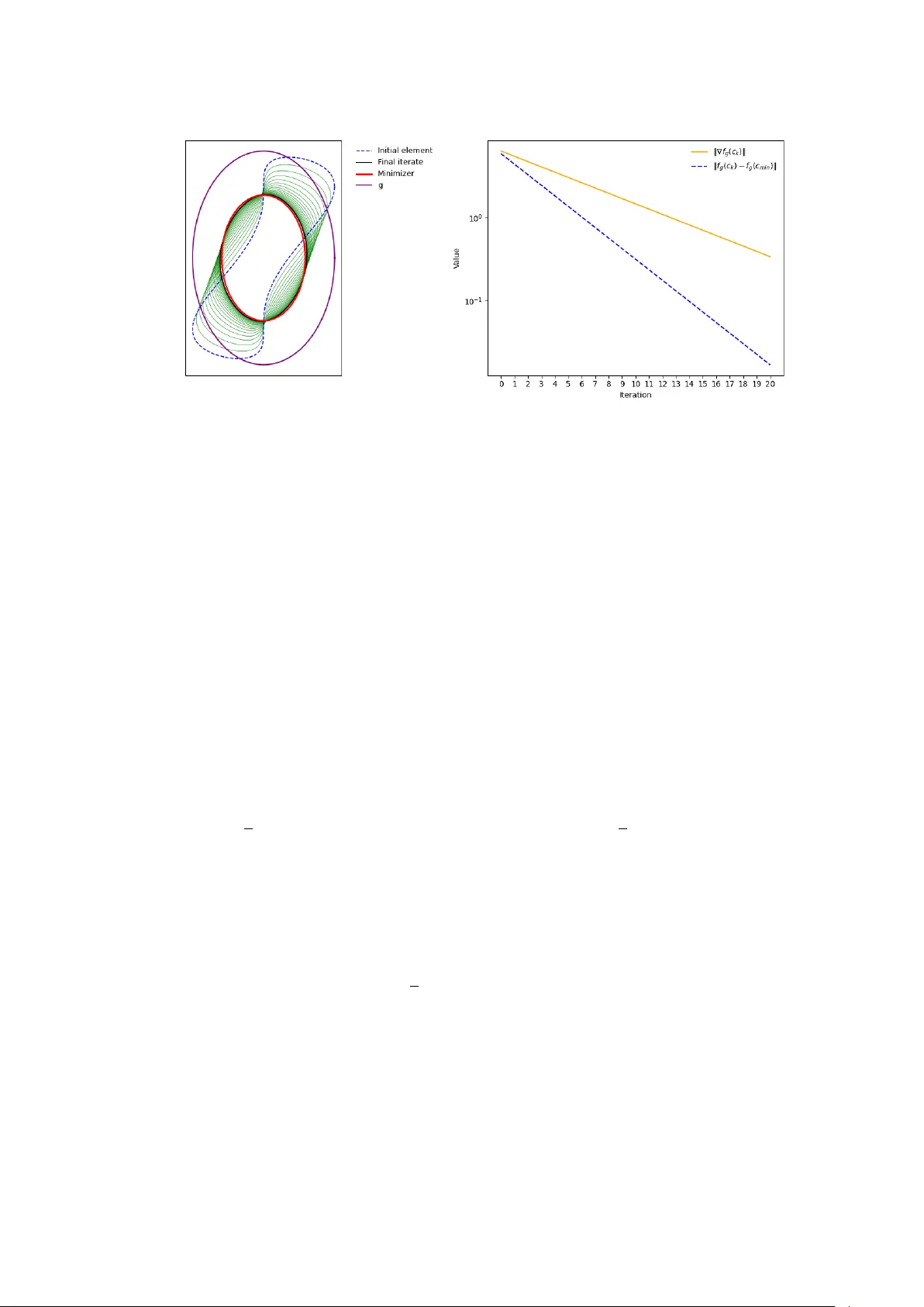
OPTIMIZA TION ON WEAK RIEMANNIAN MANIF OLDS V ALENTINA ZALBER TUS, MAX PFEFFER, AND ALEXANDER SCHMEDING Abstract. Riemannian structures on inﬁnite-dimensional manifolds arise naturally in shap e analysis and shap e optimization. These applications lead to optimization problems on manifolds whic h are not modeled on Banach spaces. The present article dev elops the basic framew ork for optimization via gradien t descent on weak Riemannian manifolds leading to the notion of a Hesse manifold. F urther, foundational prop erties for optimiza- tion are established for several classes of weak Riemannian manifolds connected to shap e analysis and shape optimization. Contents 1. In tro duction 1 2. Preliminaries 4 3. W eak Riemannian Manifolds in Optimization 5 4. Optimalit y Conditions 7 4.1. First-Order Optimality Conditions 8 4.2. Second-Order Optimality Conditions 8 5. The Riemannian Gradien t Descen t Metho d 12 6. Classes of Hesse manifolds and their Optimization-relev ant prop erties 15 6.1. Robust Riemannian manifolds 16 6.2. Strong Riemannian manifolds 19 7. Computation of the Riemannian gradien t and the Riemannian Hessian 20 8. Numerical Exp erimen ts 22 App endix A. Spra ys, connections and metrics 25 References 26 1. Introduction In recent y ears, standard ﬁrst and second order metho ds from con tinuous optimization in euclidean space ha v e b een generalized to Riemannian manifolds, thus kic kstarting the v ery activ e ﬁeld of Riemannian optimization. In particular, m uch researc h has b een done for matrix manifolds [ 1 , 8 ]. Ev en nonsmo oth optimization on smo oth Riemannian manifolds has b een studied extensiv ely [ 9 , 39 ]. In higher-dimensions, it has b een recognized that tensor trees form Riemannian manifolds, allowing for the adaptation of metho ds on matrix manifolds [ 21 ]. Ho wev er, things are muc h less clear when it comes to Riemannian manifolds of inﬁnite dimension. F or the sp ecial case of Hilbert manifolds, optimization using gradien t descen t is classical, see, e.g., the literature ov erview in [ 40 ]. There are natural geometric applications for gradients and their ﬂows on Hilb ert (sub-)manifolds: morse theory [ 33 , 35 ], energy functionals [ 10 ] for knot deformations, optimal transp ort on W asserstein space (see e.g. Date : March 27, 2026. 2020 Mathematics Subje ct Classiﬁc ation. 49K27, 58B20, 58C20, 90C48, 58D30, 49Q10. K ey wor ds and phr ases. (weak) Riemannian manifold, inﬁnite-dimensional optimization, ﬁrst-order con- ditions, v ariational analysis, shap e analysis, shap e optimization. 1 2 V ALENTINA ZALBER TUS, MAX PFEFFER, AND ALEXANDER SCHMEDING [ 2 , 27 , 32 ] for discussions). Beyond Hilb ert manifolds gradient descent techniques t ypically use conjugate gradien ts in reﬂexive Banac h spaces, see e.g. [ 13 , 14 , 42 ]. In the present article w e discuss basic theory for optimization on inﬁnite-dimensional manifolds using gradients and Hessians b eyond the setting of Hilb ert manifolds. One of sev eral challenges arising in the passage to inﬁnite-dimensions is the split b et ween diﬀeren t regimes of Riemannian geometry: Hilb ert manifolds admit str ong Riemannian metrics but manifolds mo deled on more general spaces only admit we ak Riemannian metrics, see [ 37 ]. F or the strong Riemannian metrics, the theory dev elops along the ﬁnite-dimensional lines, see e.g. [ 12 , 20 , 33 ]. Since inﬁnite-dimensional manifolds are not lo cally compact, extra conditions (e.g. P alais-Smale condition (C), [ 35 ]) are required to ensure con v ergence of the gradient sequences. Second order theory using the Riemannian Hessian gets more in volv ed on Hilb ert manifolds. Bey ond Hilb ert manifolds, ev ery Riemannian metric is necessarily a w eak Riemannian metric, i.e., the induced inner pro ducts on the tangen t spaces are only contin uous and do not induce the native top ology . Ev en on an op en subset of an inﬁnite-dimensional Hilb ert space, the inner pro duct induced b y a weak Riemannian metric is in general not equiv alent to the Hilb ert space pro duct of the model space. W eak Riemannian metrics arise in man y applications. W e list sev eral settings where gradients, gradient ﬂo ws and questions from optimization are of central interest in an inﬁnite-dimensional setting: ‚ As pioneered by V.I. Arnold, certain partial diﬀeren tial equations (PDEs) lift to geo desic equations on manifolds of Sob olev mappings (cf. [ 37 , Chapter 7]). These are Hilb ert manifolds with weak Riemannian metrics, cf. e.g. [ 32 ]. ‚ Shap e analysis studies inv ariant metrics and ﬂo ws on weak Riemannian manifolds of mappings and diﬀeomorphism groups, cf. e.g. [ 5 , 28 , 30 , 31 , 43 ]. Here optimization is relev an t in large deformation diﬀeomorphic metric matching (LDDMM), [ 41 ]. See e.g. [ 4 ] for a concrete example inv olving the gradien t ﬂow. ‚ Shap e optimization studies gradients for w eak Riemannian metrics on inﬁnite- dimensional manifolds, see e.g. [ 25 , 26 ]. ‚ (time-)evolving embedded man ifolds and ev olution equations on them lead to gra- dien t ﬂo ws on w eak Riemannian manifolds. The curve-shortening ﬂow studied by Gage and Hamilton and related ﬂows are of this t ype, cf. [ 15 , 38 ] The state of the art to treat these problems is to emplo y one of the follo wing strategies: T reat the qualitativ e b eha viour of gradien t ﬂows. F or example for time-ev olving and shap e manifolds, developmen t of singularities of the gradient ﬂows and geo desic equations are studied without directly employing numerical metho ds, [ 15 , 32 ]. F or optimization sc hemes base on inﬁnite-dimensional manifolds, there are t w o main approac hes: In many relev an t examples, the inﬁnite-dimensional gradien t equations can be translated to ﬁnite-dimensional (partial) diﬀeren tial equations. These are then numerically solv ed using PDE metho ds (e.g. [ 6 , 25 , 26 ]). In the Hilb ert manifold setting, discretisation of the equations are applied together with conditions assuring conv ergence and con v ergence rate, see e.g. [ 12 , 33 , 40 ]. These tec hniques hav e b een generalised to Banach manifolds (e.g. [ 10 , 13 , 14 , 41 , 42 ]) using w eaker notions of gradients and dualities not necessarily induced by (weak) Riemannian metrics. These approac hes either require strong settings (strong metrics, Hilbert manifolds) or exploit connections to ﬁnite dimensional geometry for the discretisation and computation of the descent sc heme. T o the b est of our kno wledge, a general in v estigation of basic optimization algorithms for w eak Riemannian manifolds is so far missing. One aim of the presen t article is to provide an introduction to basic optimization tec h- niques on inﬁnite-dimensional manifolds in the weak setting. W e highligh t pitfalls and OPTIMIZA TION ON WEAK RIEMANNIAN MANIFOLDS 3 c hallenges arising on Riemannian manifolds b eyond the Hilb ert setting. F urther, funda- men tal optimality conditions and conv ergence results for optimization on weak Riemann- ian manifolds are provided. While m uc h of the classical in tuition from ﬁnite-dimensional optimization (as presen ted in [ 8 ]) carries ov er, the absence of the Hilb ert/Banach space structure mak es it a priori unclear, in which sense standard optimalit y conditions gener- alise to w eak Riemannian manifolds. Theorem 1.1 (First-Order Optimalit y) . L et f : M Ñ R b e c ontinously diﬀer entiable on a we ak R iemannian manifold M . Then every lo c al minimizer p P M satisﬁes ∇ f p p q “ 0 , wher e ∇ f denotes R iemannian gr adient of f . This recov ers the familiar necessary condition from ﬁnite-dimensional optimization [ 8 ]. T o extend ﬁrst-order optimality conditions to algorithms, we show that under an addi- tional assumption ensuring suﬃcient structure on weak Riemannian manifolds, the clas- sical ﬁnite-dimensional conv ergence result for the Riemannian gradient descen t [ 8 ] carries o ver to our presen t setting. Theorem 1.2. A l l ac cumulation p oints of the se quenc e of iter ates p p n q n P N gener ate d by the Riemannian desc ent algorithm ar e critic al p oints, and lim n Ñ8 ~ ∇ f p p n q~ “ 0 . wher e ~ ¨ ~ is the norm induc e d by the we ak Riemannian metric. Second order optimality is more complicated due to intricate structure arising in the critical p oints of the Hessian (cf. e.g. Theorem 7.6). Nevertheless, one can pro ve the follo wing: Theorem 1.3 (Second-Order Optimality) . A p oint p P M with ∇ f p p q “ 0 and Hess f p p q p ositive-deﬁnite is a lo c al minimizer if and only if the R iemannian Hessian is c o er cive at that p oint, i.e. ther e exists µ ą 0 such that g p p Hess f p p qr v s , v q ě µ ~ v ~ p , @ v P T p M . Unlik e the ﬁnite-dimensional setting–where p ositiv e deﬁniteness of the Hessian suﬃces– co ercivit y is more restrictiv e here, failing to follo w from p ositiv e deﬁniteness on w eak Riemannian manifolds. Note that this describ es a t ypical phenomenon b ey ond Hilb ert spaces. F or example it is w ell known that conv exit y prop erties on functions used in ﬁnite dimensional optimization, typically force a Banach space to either b e reﬂexive or ev en a Hilb ert space (see e.g. [ 7 , 16 ]). T o establish second-order optimalit y conditions that pro vide, in addition to necessary conditions, a suﬃcient condition for local minima, w e require several additional properties of the underlying weak Riemannian manifold. These prop erties ensure that the Hessian is w ell behav ed and allo w us to dra w conclusions ab out lo cal extrema. A w eak Riemannian manifold satisfying these properties will be called a Hesse manifold . W e sho w that Hesse manifolds constitute a reﬁnement of the existing classiﬁcation in to w eak, robust, and strong Riemannian manifolds. In particular, we demonstrate that: Theorem 1.4. Every r obust R iemannian C 8 - manifold p M , g q is a Hesse manifold. W e then study the robust metrics introduced in [ 28 ] with resp ect to their application in optimization. As a new result, w e prov e that the class of elastic metrics from shap e analysis are robust. Summing up, this leads to the following hierarc h y of Riemannian manifolds: 4 V ALENTINA ZALBER TUS, MAX PFEFFER, AND ALEXANDER SCHMEDING (p ossibly) Inﬁnite-Dimensional manifold Examples Strong Riemannian Robust Riemannian Hesse manifold W eak Riemannian dim ă 8 paracompact Grossmann’s ellipsoid Theorem 6.12 L 2 -metric; elastic metric Theorem 6.7; Theorem 6.8 t wisted ℓ 2 Theorem 3.4 Hilb ert Manifold The structure of the article is as follo ws: T o establish Riemannian optimization on w eak Riemannian manifolds, w e ﬁrst address the primary structural c hallenges. Section 3 in tro duces tw o fundamental restrictions enabling Riemannian optimization in this gen- eralit y , presents examples of pathological b eha vior without them, and veriﬁes that these restrictions preserve the essen tial structure of weak Riemannian manifolds. Building on this foundation, Section 4 derives ﬁrst- and second-order optimality condi- tions in terms of the Riemannian gradient and Hessian. Section 5 in tro duces the Riemann- ian gradient descent metho d and analyzes its conv ergence, showing that classical results carry ov er under mild additional conditions. W e then in tro duce tw o k ey classes - strong and robust Riemannian manifolds - fo cusing on the latter’s construction and structural prop erties (Section 6), while pro ving simpliﬁca- tions for the former. Finally , Section 7 pro vides explicit formulas for Riemannian gradients and Hessians, complemen ted b y numerical examples (Section 8). A c kno wledgemen ts V.Z. was funded by the German research foundation (DFG – Pro jektn ummer 448293816). V. Zalbertus thanks the mathematical institute at NTNU for the hospitalit y during a researc h stay while part of this w ork w as conducted. 2. Preliminaries W eak Riemannian manifolds are often mo deled on lo cally conv ex spaces whic h are in general not Banac h manifolds. The usual calculus, also called F réc het diﬀeren tiability , has to be replaced. W e emplo y Bastiani calculus, see [ 37 , Section 1.4], whic h is based on directional deriv ativ es. This means that a contin uous function f : E Ě U Ñ F on an op en subset of a lo cally con vex space is C 1 if for ev ery x P U, v P E the directional deriv ativ e d f p x ; v q : “ lim h Ñ 0 h ´ 1 p f p x ` hv q ´ f p x qq exists and yields a con tinuous map d f : U ˆ E Ñ F . Using iterated directional deriv ativ es, one likewise deﬁnes C k -mappings for k P N . A map which is C k for all k P N is called smo oth or C 8 . The usual assertions suc h as linearit y of the deriv ativ e and the c hain rule remain v alid. As the chain rule is v alid, w e can deﬁne as in ﬁnite dimensions, manifolds via c harts. A manifold is called a Hilb ert/Banach/F r é chet-manifold if all the mo delling spaces of the manifold are Hilbert/Banach/F réchet spaces. F urther, for a manifold M the tangent spaces T p M are deﬁned via equiv alence classes of curves [ 37 , Def. 1.41] and canonically isomorphic to the mo del space of the manifold. Similarly the tangent bundle and diﬀeren tiability of mappings on manifolds can b e deﬁned. F or the tangen t map of a C 1 -map f : M Ñ N we will write D p f : T p M Ñ T f p p q N , r γ s ÞÑ r f ˝ γ s . F or a v ector bundle π : E Ñ M on a smo oth manifold, we will write Γ p E q for the space of smo oth bundle sections. In the sp ecial case that E “ T M is the tangen t bundle, w e also write V p M q : “ Γ p T M q . OPTIMIZA TION ON WEAK RIEMANNIAN MANIFOLDS 5 When establishing Riemannian metrics on lo cally con vex manifolds b eyond the Hilb ert setting, a crucial distinction arises b etw een we ak and str ong Riemannian metrics, essential for the subsequen t optimization. Deﬁnition 2.1 (W eak/Strong Riemannian Manifold) . Let M be a C 1 -manifold. A we ak R iemannian metric g on M is a smo oth map g : T M ‘ T M Ñ R , p v p , w p q ÞÑ g p p v p , w p q , suc h that g p is s ymmetric, bilinear on T p M ˆ T p M , and g p p v , v q ě 0 with equality iﬀ v “ 0 . If the topology on p T p M , g p q coincides with the subspace top ology of T p M Ă T M , then g is str ong . W e then call p M , g q a we ak/str ong Riemannian manifold . Since we op erate beyond the Banac h setting, there is no natural norm on the spaces we consider. Although the inner pro ducts induce norms, these do not generate the natural top ology , and in particular, the spaces are not complete with resp ect to these norms. R emark 2.2 . T o av oid confusion, we write ~ v ~ p : “ a g p p v , v q for the norm on T p M induced b y the inner pro duct g p , whic h need not b e complete, and } v } for a Banach norm, if we are working in the Banach case. T o facilitate Riemannian optimization in our setting, w e introduce: Deﬁnition 2.3 (Riemannian Gradien t) . Let p M , g q b e a w eak Riemannian C 1 -manifold and f : M Ñ R a C 1 -map. A v ector ﬁeld ∇ f satisfying D p f p v q “ g p p ∇ f p p q , v q @ v P T p M is the R iemannian gr adient of f . Deﬁnition 2.4 (Riemannian Hessian) . Let p M , g q b e a C 2 -manifold with ﬁrst-order 1 Levi–Civita connection ∇ , and f : M Ñ R a C 2 -function with Riemannian gradien t ∇ f . The Riemannian Hessian of f at p is the map Hess f p p q : T p M Ñ T p M , v ÞÑ ∇ v ∇ f p p q . All deﬁnitions and results from inﬁnite-dimensional diﬀeren tial geometry follo w [ 37 ]. F or the readers con v enience w e recall some essential tec hnical objects in Section A. 3. Weak Riemannian Manifolds in Optimiza tion T o in tro duce the subsequen t chapters on optimization on weak Riemannian manifolds, w e ﬁrst specify the setting in whic h Riemannian optimization techniques can b e applied. Although the ob jective of this work is to develop optimization methods on spaces as general as p ossible - namely weak Riemannian manifolds - the weak structure of the underlying geometry requires us to impose sev eral structural assumptions in order to establish a w ell-deﬁned framew ork. Since our optimization approac h relies on Riemannian methods, we fo cus on ﬁrst- and second-order diﬀerential ob jects, in particular the Riemannian gradien t and the Riemann- ian Hessian. These quantities are essential for the form ulation and analysis of ﬁrst- and second-order optimality conditions and gradient-based optimization algorithms. On w eak Riemannian manifolds, how ev er, these ob jects are not a v ailable in general. Recall that for a weak Riemannian C 1 - manifold p M , g q the Riemannian gradient of a C 1 - function f is deﬁned by the unique vector ﬁeld satisfying D p f p v q “ g p p ∇ f p p q , v q for all v P T p M . Since on weak Riemannian manifolds the musical morphism b et ween the tangen t bundle and it’s dual isn’t necessarily surjective [ 37 , 4.4], the existence of the Riemannian gradien t of a function cannot b e guaran teed. The following example 1 a connection is ﬁrst order if its v alue at a point dep ends at most on the 1 -jets of the sections at the p oin t. See Remark 4.5. Ev ery connection on a ﬁnite dimensional manifold is of ﬁrst order. 6 V ALENTINA ZALBER TUS, MAX PFEFFER, AND ALEXANDER SCHMEDING demonstrates a situation in which the Riemannian gradien t fails to exist on the tangent space under consideration. Example 3.1. W e consider the space Imm p S 1 , R 2 q of all smo oth immersions with the in v ariant H 1 ´ metric: g H 1 inv ,c p u, v q : “ g inv ,c p u, v q ` g inv ,c p 9 u, 9 v q . In [ 37 , Section 4] it has b een sho wn, that ` Imm p S 1 , R 2 ˘ , g H 1 inv ,c ˘ is indeed a w eak Riemannian manifold. W e then consider the length functional L : Imm p S 1 , R 2 q Ñ R , L p c q : “ ż S 1 | 9 c | dµ. In [ 38 , Section 4.1] the in v ariant H 1 -gradien t of the length functional L was computed using a Green’s function to solv e the arising ODE. Using the arc-length reparametrisation for c , we write γ : r 0 , L s Ñ R 2 , s ÞÑ c p exp p i s { 2 π q with L : “ L p c q and the Riemannian gradien t becomes: ∇L p s q “ γ p s q ` ż L 0 γ p t q cosh ` | s ´ t | ´ L 2 ˘ 2 sinh ` ´ L 2 ˘ dt. (1) No w (1) will in general not b e diﬀerentiable in s (i.e. in the con tribution b y Green’s func- tion), whence the Riemannian gradien t of L do es not exist as an elemen t in T Imm p S 1 , R 2 q (or for that matter in the tangent space of the one time contin uously diﬀerentiable im- mersion which is the context studied in [ 38 ]). Here the gradien t only exists as an elemen t in the completion of the tangen t space, which can b e identiﬁed with the space H 1 p S 1 , R 2 q of all Sob olev H 1 -functions. R emark 3.2 . The gradient ﬂow induced b y the length functional with resp ect to the in- v ariant L 2 -metric corresp onds to the famous curve shortening ﬂo w studied in [ 15 ]. With resp ect to the in v arian t H 1 -metric, the corresp onding gradient ﬂo w has been studied in [ 38 ]. Nev ertheless, assuming the existence of a Riemannian gradient does not turn out to b e o verly restrictive, since it’s existence do es not, for instance, imply that the metric is strong. In Section 7, we present several examples illustrating the computation of Riemannian gradien ts on weak Riemannian manifolds. In particular, Example 7.5 provides an explicit computation of the Riemannian gradien t of the length functional L on the space of smo oth immersion Imm p S 1 , R 2 q endow ed with the in v arian t L 2 ´ metric, thereb y demonstrating that the existence of the Riemannian gradien t of a function dep ends not only on the function itself but also on the c hosen metric. In the context of Riemannian optimization, where the structure of the Riemannian gra- dien t is essential, but cannot b e guaran teed when w orking on weak Riemannian manifolds, w e in troduce the following deﬁnition for notational con v enience. Deﬁnition 3.3. A C 1 - function f : M Ñ R on a w eak Riemannian C 1 - manifold p M , g q is called a gr adient-admitting function (abbreviated gaf ) if the Riemannian gradient ∇ f p p q exists for all p P M . In addition to the Riemannian gradient, the Riemannian Hessian enco des second-order information ab out the lo cal b eha vior of the function. Consider a w eak Riemannian C 8 - manifold M that admits a ﬁrst-order Levi-Civita connection ∇ . F or a gradient-admitting C 2 - function f on M , recall, that the Riemannian Hessian of f at p P M is deﬁned b y Hess f p p qr u s “ ∇ u ∇ f , u P T p M . Consequen tly , the deﬁnition of the Riemannian Hessian requires not only the existence of the Riemannian gradient but also the av ailability of a ﬁrst-order Levi-Civita connection. OPTIMIZA TION ON WEAK RIEMANNIAN MANIFOLDS 7 This imposes an additional structural restriction on the underlying manifold. In particular, on w eak Riemannian manifolds such a connection do es not exist in general. An explicit example of a w eak Riemannian manifold without a Levi-Civita connection is giv en in [ 5 , p.12]. Ho wev er, the existence of a Levi-Civita connection alone is still not suﬃcien t for our sub- sequen t analysis. In order to carry basis-indep enden t arguments, w e additionally require the existence of a metric spra y , cf. Section A. A spray is a second order vector ﬁeld whic h, when compatible with the metric, pla ys the same role as the Christoﬀel symb ols. Suc h a spra y not only induces a ﬁrst-order Levi-Civita connection, but also pro vides the co v ari- an t deriv ativ e structure necessary for intrinsic arguments. Similiarly to the Levi-Civita connection, a metric spray do es not exist on weak Riemannian manifolds in general. Example 3.4. Consider the Hilb ert space M “ ` ℓ 2 , x¨ , ¨y ˘ of all square-summable real sequences equipp ed with the weak Riemannian metric g : T ℓ 2 ‘ T ℓ 2 Ñ R , T p ℓ 2 ˆ T p ℓ 2 Q ` p x n q n , p y n q n ˘ ÞÑ e ´} p } 2 ÿ n P N x n y n n 3 . As shown in [ 37 , 4.22], this metric does not admit a metric spra y . By contrast, [ 37 , 5.7] computes the metric spra y for a large class of w eak Riemannian manifolds of the form ` C 8 p S 1 , M q , g L 2 ˘ , where p M , g q is a strong Riemannian manifold and g L 2 denotes the induced L 2 metric, sho wing that this additional assumption do es not imply that the metric is strong. Ho wev er, Example 3.4 demonstrates that additional structural assumptions are neces- sary to ensure the existence and w ell-p osedness of the Riemannian Hessian. Accordingly , the follo wing deﬁnition establishes notation and identiﬁes the class of w eak Riemannian manifolds considered in this w ork. Deﬁnition 3.5. A w eak Riemannian C 8 - manifold p M , g q is called a Hesse manifold if it admits a metric spra y S g . 4. Optimality Conditions In this c hapter, w e derive ﬁrst- and second-order optimality conditions for optimiza- tion on w eak Riemannian manifolds under the structural assumptions introduced in the previous c hapter. The goal is to show that, once these restrictions are imp osed, the local optimalit y theory closely parallels the one on strong- or ﬁnite-dimensional Riemannian manifolds. Our exp osition follo ws the framework dev elop ed by Boumal in [ 8 ] for ﬁnite-dimensional Riemannian manifolds. W e adopt his deﬁnition of critical p oin ts, Riemannian gradien ts and Riemannian Hessians, and adapt the corresp onding arguments to the presen t setting of w eak Riemannian manifolds. In particular, we sho w that under the stated assump- tions, ﬁrst-order necessary optimality conditions can b e form ulated in terms of v anishing Riemannian gradients. While second-order conditions in the ﬁnite-dimensional setting t ypically only require p ositive deﬁniteness of the Riemannian Hessian to guaran tee a lo cal minim um, in the inﬁnite-dimensional setting considered here p ositive deﬁniteness alone is not suﬃcient. Instead, an additional requiremen t is needed: the Riemannian Hessian m ust b e co ercive at the p oin t of interest. These results justify the use of classical opti- mization intuition in the more general weak Riemannian setting for ﬁrst-order conditions; ho wev er, this intuition do es not carry o ver to second-order conditions, where additional assumptions and analytical to ols are required to rigorously establish lo cal optimality . Throughout this c hapter, p M , g q denotes a w eak Riemannian C 1 -manifold. 8 V ALENTINA ZALBER TUS, MAX PFEFFER, AND ALEXANDER SCHMEDING 4.1. First-Order Optimality Conditions. As a ﬁrst step tow ards establishing opti- mization conditions on w eak Riemannian manifolds, we consider the notion of critical p oin ts. In the ﬁnite-dimensional and strong Riemannian setting, critical p oints are char- acterized by the v anishing of the Riemannian gradien t and are directly linked to ﬁrst-order necessary conditions. In the present weak Riemannian setting, ho w ev er, this characterization is not immedi- ate, as the deﬁnition of diﬀerentials and tangent spaces relies on Bastiani calculus rather than on a Hilb ert space structure. W e therefore b egin b y v erifying that Boumal’s deﬁnition of critical p oin ts is compatible with the diﬀeren tial structure adopted here. Deﬁnition 4.1. Let f : M Ñ R b e a C 1 -map. A p oint p P M is called a critic al p oint of f , if p f ˝ γ q 1 p 0 q ě 0 for all C 1 -curv es γ on M passing through p . Despite the w eak Riemannian structure, critical p oin ts admit the same c haracterization as in the ﬁnite-dimensional setting: critical points can be c haracterized equiv alen tly by the v anishing of the diﬀeren tial and by the v anishing of the Riemannian gradient. The calcu- lations are the same as in the ﬁnite dimensional setting and, for the readers con v enience, w e highligh t only where the w eak structure is needed. Prop osition 4.2. Let f : M Ñ R b e C 1 and p P M . The p oint p is a critical p oint of f if and only if (1) D p f p v q “ 0 for all v P T p M , (2) ∇ f p p q “ 0 if f is a gaf. Finally , ev ery lo cal minimizer of f is a critical p oin t. Pr o of. The equiv alence to (1) and the addendum can b e prov ed exactly as in the ﬁnite dimensional case. See e.g. [ 8 , Proposition 4.5.] whic h only uses the con tin uit y of f ˝ c for a smo oth curve c on M . F or (2) we observ e that as D p f p v q “ g p p ∇ f p p q , v q “ 0 , @ v P T p M , (2) w e see that (1) implies (2) as a weak Riemannian metric is non-degenerate and thus (2) implies that the gradient v anishes if and only if p is critical. □ This result enables us to establish the fundamen tal link betw een minimizers and critical p oin ts. Consequen tly , the classical ﬁrst-order necessary optimalit y condition remains v alid in the weak Riemannian framework considered here. This provides the foundation for the second-order analysis dev elop ed below. 4.2. Second-Order Optimality Conditions. W e now establish suﬃcient second-order optimalit y conditions on Hesse manifolds, that is, manifolds equipp ed with a Levi-Civita connection induced by a metric spray . The metric spray framework allows us to deﬁne co v ariant deriv ativ es of v ector ﬁelds along curv es in a basis-indep enden t manner. This in trinsic notion of diﬀerentiation is crucial for formulating a second-order T aylor expan- sion of functions along suitable curv es without assuming the existence of a basis of the underlying vector space. W e sho w that, unlik e in the ﬁnite-dimensional setting where p ositive deﬁniteness of the Riemannian Hessian alone suﬃces, a critical p oin t must not only admit a p ositive deﬁnite Hessian but also satisfy a co ercivit y condition in order to b e a strict lo cal mini- mizer. This highlights an imp ortan t distinction b etw een ﬁnite-dimensional optimization and optimization in the w eak Riemannian setting. W e brieﬂy recall the deﬁnition of the Riemannian Hessian for conv enience. Deﬁnition 4.3. Let p M , g q b e a Hesse-manifold and f : M Ñ R b e a C 2 - gaf. Then the Riemannian Hessian of f at p P M is deﬁned as follows: Hess f p p q : T p M Ñ T p M u ÞÑ ∇ u ∇ f . OPTIMIZA TION ON WEAK RIEMANNIAN MANIFOLDS 9 T o relate the Riemannian Hessian to local minimalit y , we analyze the second-order expansion of f along smo oth curves. Let c : I Ñ M b e a smo oth curve with c p 0 q “ p , and deﬁne g “ f ˝ c . Since g : I Ñ R is a classical C 2 - function, w e ha v e the standard T aylor expansion f p c p t qq “ g p t q “ g p 0 q ` tg 1 p 0 q ` t 2 2 g 2 p 0 q ` O p t 3 q . (3) The ﬁrst deriv ative follows from the c hain rule: g 1 p t q “ D c p t q f p c 1 p t qq “ g c p t q ` ∇ f p c p t qq , c 1 p t q ˘ . (4) In particular, p f ˝ c q 1 p 0 q “ g p ` ∇ f p p q , c 1 p 0 q ˘ . Th us, ﬁrst-order b ehavior is completely determined by the Riemannian gradient. T o compute the second deriv ativ e g 2 p t q , we m ust diﬀerentiate g c p t q ` ∇ f p c p t qq , c 1 p t q ˘ . This requires a notion of diﬀerentiation of vector ﬁelds along curves. Those vector ﬁelds are deﬁned analogously to [ 8 , Deﬁnition 5.28.] as follows: Deﬁnition 4.4. Let M b e a manifold and c : I Ñ M b e a curv e on M . A (smo oth) map Z : I Ñ T M is called a (smo oth) ve ctor ﬁeld on c if Z p t q P T c p t q M for all t P I . The set of all smo oth vector ﬁelds on c is denoted b y V p c q . T o make sense of diﬀeren tiation of vector ﬁelds on curves, we require an appropriate op erator with certain prop erties. Since not all v ector ﬁelds Z P V p c q are of the form X ˝ c for some X P V p M q , we cannot simply use the Levi-Civita connection on M and must in tro duce a diﬀeren t concept for diﬀerentiating suc h v ector ﬁelds. This is precisely where the metric spra y structure b ecomes essen tial. R emark 4.5 . It is a standard argumen t that every connection ∇ on a ﬁnite-dimensional v ector bundle is of ﬁrst or der in the sense that for section X , Y and m P M , the v alue ∇ X Y p m q dep ends only on the v alue X p m q and the ﬁrst order jet of Y . Unfortunately , the ﬁnite-dimensional pro of do es not generalise without further assumptions. One can prov e that ev ery connection asso ciated to a spra y , cf. Section A, is a ﬁrst order connection in this sense. It is unkno wn whether there exist connections on inﬁnite-dimenisonal manifolds whic h are not of ﬁrst order. If the Levi–Civita connection is induced b y a metric spray , then one obtains a canonical diﬀeren tiation operator along curves called the c ovariant derivative along c . Theorem 4.6. L et p M , g q b e a Hesse-manifold. F or every smo oth curve c : I Ñ M , ther e exists a unique op er ator D d t : V p c q Ñ V p c q , c al le d the c ovariant derivative along c, that satisﬁes the fol lowing pr op erties for al l Y , Z P V p c q , X P V p M q , g P C 1 p I , R q and a, b P R : (1) R -linearity: D d t ` aY ` bZ ˘ “ a D d t Y ` b D d t Z, (2) Leibniz rule: D d t ` g Z ˘ “ g 1 Z ` g D d t Z, (3) Chain rule: ` D d t ` X ˝ c ˘˘ p t q “ ∇ c 1 p t q U for all t P I . (4) Pro du ct rule: d d t g p Y , Z q “ g p D d t Y , Z q ` g p Y , D d t Z q , where g p Y , Z q P C 1 p I , R q is deﬁned by g p Y , Z qp t q “ g c p t q p Y p t q , Z p t qq . Pr o of. The existence and uniqueness of suc h an op erator follo ws from Prop osition 4.36 in [ 37 ]. The construction presented there is based on the metric spray and yields a cov arian t deriv ative along curv es satisfying properties (i)–(iv). □ 10 V ALENTINA ZALBER TUS, MAX PFEFFER, AND ALEXANDER SCHMEDING R emark 4.7 . In the ﬁnite-dimensional setting, analogous constructions are often carried out using lo cal frames and co ordinate represen tations, as for instance done by Boumal in [ 8 , Theorem 5.29.]. Suc h arguments rely on the existence of ﬁnite-dimensional bases of the tangent spaces. In contrast, the presen t approach is based on the spra y-induced connection and do es not require the use of lo cal frames. The diﬀeren tiation op erator along curv es is constructed in trinsically , without resorting to basis expansions. This makes the argument directly applicable in the weak inﬁnite-dimensional Riemannian setting considered here. T o relate the Riemannian Hessian to the second-order expansion along curv es, we ex- press it in terms of the induced co v arian t deriv ative. Let c : I Ñ M b e a smo oth curve with c p 0 q “ p and c 1 p 0 q “ v . By the c hain rule for the induced co v ariant deriv ative along c, we obtain Hess f p p qr v s “ ∇ v ∇ f “ D d t ∇ f p c p t qq | t “ 0 . (5) Using the representation of the Riemannian Hessian in terms of the induced cov arian t deriv ative (5) and the structural prop erties established in Theorem 4.6, the computation of the second deriv ative of g “ f ˝ c proceeds exactly as in the ﬁnite-dimensional case in [ 8 , 5.9]. As the argumen t uses only structural properties of the cov ariant deriv ative, it remains v alid in the present weak Riemannian framework. Hence, g 2 p t q “ g c p t q ` Hess f p c p t qqr c 1 p t qs , c 1 p t q ˘ ` g c p t q ` ∇ f p c p t qq , c 2 p t q ˘ . (6) Consequen tly , the second-order T aylor expansion of f ˝ c is giv en by f p c p t qq “ f p p q ` tg p ` ∇ f p p q , v ˘ ` t 2 2 g p ` Hess f p p qr v s , v ˘ ` t 2 2 g p ` ∇ f p p q , c 2 p 0 q ˘ ` O p t 3 q . (7) Ha ving expressed the second-order T aylor expansion in terms of the Riemannian gradient and the Riemannian Hessian, w e now adopt the notion of second-order critical p oints as in tro duced in the ﬁnite-dimensional setting by Boumal [ 8 , Section 6.1]. These p oints will b e sho wn to coincide precisely with the local minimizers of a function, if in addition the Riemannian Hessian at these points is coercive. Establishing this result relies on the second-order T aylor expansion of f ˝ c (cf. (7)). Deﬁnition 4.8. Let M b e a C 2 - manifold and f : M Ñ R b e a C 2 - function. A p oin t p P M is called a se c ond-or der critic al p oint for f if it is a critical p oint and p f ˝ c q 2 p 0 q ě 0 for all smo oth curves c on M such that c p 0 q “ p . In direct analogy of the ﬁnite-dimensional case [ 8 , Prop osition 6.3.], one can sho w, that critical p oints are exactly the p oin ts where the Riemannian gradient v anishes and the Riemannian Hessian is p ositiv e semi-deﬁnite. The pro of carries ov er directly to the weak Riemannian setting, as it relies solely on the ﬁrst and second deriv ativ es of f ˝ c , which w e ha v e established in (4) and (6). Prop osition 4.9. Let f : M Ñ R b e a smo oth gaf on a Hesse manifold M . Then, x is a second-order critical p oin t if and only if ∇ f p x q “ 0 and Hess f p x q ľ 0 . W e now turn to the pro of of the main result. While the Riemannian gradient con- dition pro vides a necessary criterion, this theorem go es further b y establishing when a critical p oin t is indeed a minimizer. This result demonstrates that in tuition from ﬁnite- dimensional optimization do es not directly carry o ver to the more general setting of weak Riemannian manifolds and must b e applied with caution. OPTIMIZA TION ON WEAK RIEMANNIAN MANIFOLDS 11 Prop osition 4.10. Let p M , g q b e a Hesse manifold and let f : M Ñ R b e a C 2 -gaf. F or p P M , suppose that the Riemannian Hessian is co ercive, i.e. there exists µ ą 0 suc h that g p p Hess f p p qr v s , v q ě µ ~ v ~ 2 p , @ v P T p M . (8) Then, any strict second-order critical point of f is a strict lo cal minimizer. Pr o of. Let ϕ : U ϕ Ñ V ϕ b e a chart around p with ϕ p p q “ 0 . Since V ϕ is an op en subset of a lo cally conv ex space, there exists an op en con vex neigh b orho o d W ϕ Ă V ϕ con taining 0 . F or an y x P W ϕ , deﬁne a smo oth curv e on M via c p t q : “ ϕ ´ 1 p tx q . By the second-order T aylor expansion of f along c (cf. (7)) and the fact that p is a critical p oint, w e obtain f p c p t qq “ f p p q ` t 2 2 g p ` Hess f p p qr c 1 p 0 qs , c 1 p 0 q ˘ ` R p t q , where R p t q “ O p t 3 q , i.e. lim t Ñ 0 R p t q{ t 3 “ 0 . By the co ercivity of the Hessian at p , w e hav e g p ` Hess f p p qr c 1 p 0 qs , c 1 p 0 q ˘ ě µ ~ c 1 p 0 q~ 2 p “ µ   D ϕ p p q ϕ ´ 1 p x q   2 p , and therefore f p c p t qq ě f p p q ` t 2 µ 2   D ϕ p p q ϕ ´ 1 p x q   2 p ` R p t q . (9) On E ϕ w e deﬁne a norm as follo ws: ~ x ~ ϕ : “ b g p ` D ϕ p p q ϕ ´ 1 p x q , D ϕ p p q ϕ ´ 1 p x q ˘ , x P E ϕ . By construction, with resp ect to this norm, the linear mapping D ϕ p p q ϕ ´ 1 : ` E ϕ , ~ ¨ ~ ϕ p p q ˘ Ñ ` T p M , g p ˘ is contin uous, where w e identiﬁed T ϕ p p q V ϕ – E ϕ . Bounding b y the operator norm A ą 0 ,   D ϕ p p q ϕ ´ 1 p x q   2 p ď A 2 ~ x ~ 2 ϕ p p q for all x P W ϕ . Since R p t q “ O p t 3 q , there exists ξ ą 0 suc h that | R p t q| ď t 2 2 µA 2 for all t P p 0 , min t 1 , ξ uq . Using (9), we obtain f p c p t qq ě f p p q ` t 2 µ 2 A 2 ` R p t q ě f p p q ` t 2 µ 2 A 2 ~ x ~ 2 ϕ p p q ´ t 2 µ 2 A 2 “ f p p q ` t 2 µ 2 A 2 p~ x ~ 2 ϕ p p q ´ 1 q . No w restrict to x P W ϕ with ~ x ~ ϕ p p q ă 1 . Then ~ x ~ 2 ϕ p p q ´ 1 ă 0 , and thus f p c p t qq ą f p p q for all t P p 0 , min t 1 , ξ uq and all x P W ϕ with 0 ă ~ x ~ ϕ p p q ă 1 . Deﬁne Y ϕ : “ ! ϕ ´ 1 p tx q ˇ ˇ ˇ t P p 0 , min t 1 , ξ uq , x P W ϕ , ~ x ~ ϕ p p q ă 1 ) . Since ϕ is a homeomorphism and the set t tx | t P p 0 , min t 1 , ξ uq , x P W ϕ , ~ x ~ ϕ p p q ă 1 u is op en in V ϕ with resp ect to the lo cally conv ex top ology , the set Y ϕ is op en in M . By the preceding estimate, we hav e f p q q ą f p p q for all q P Y ϕ , so p is a strict lo cal minimizer of f . □ R emark 4.11 . The coercivity of the Riemannian Hessian represents a k ey diﬀerence com- pared to the ﬁnite-dimensional case. This is w ell kno wn, see e.g. [ 11 ] for the use of co ercivit y conditions on Banac h manifolds in relation to P alais and Smales condition (C). Condition (C) replaces compactness arguments which are not a v ailable in our setting. In particular, coercivity do es not follow from the p ositive deﬁniteness of the Riemannian Hessian and m ust therefore b e assumed separately . 12 V ALENTINA ZALBER TUS, MAX PFEFFER, AND ALEXANDER SCHMEDING Ha ving established ﬁrst- and second-order optimalit y conditions on w eak Riemannian manifolds, w e now turn to a concrete descent metho d. In Section 8, we will apply these optimalit y conditions to speciﬁc examples alongside this metho d. 5. The Riemannian Gradient Descent Method In this c hapter, we introduce a basic descen t metho d, namely the Riemannian gradient descen t (RGD) algorithm, and establish conv ergence results for this metho d. Before we can state the algorithm, w e need an auxiliary structure. In ﬁnite dimensional optimization on manifolds [ 8 , Chapter 3.6] one deﬁnes Deﬁnition 5.1. A smo oth map R : T M Ñ M is called a r etr action if for every v P T M the smo oth curve c v p t q : “ R p tv q satisﬁes c p 0 q “ x and 9 c p 0 q “ v . W e deviate slightly from lo c.cit. and will allo w retractions deﬁned only on an op en neigh b orho o d Ω of the zero-section in T M . How ev er, even with this relaxation, w e will see that retractions are not suﬃcient as the next example shows. Example 5.2. Let S 1 Ď R 2 b e the unit circle. W e recall from [ 37 , Example 3.8] that the diﬀeomorphism group Diﬀ p S 1 q is an inﬁnite-dimensional Lie group not mo delled on a Banac h space. The tangent bundle of the Lie group is trivial, [ 37 , Lemma 3.12 (b)], i.e. the group m ultiplication m induces a diﬀeomorphism Φ ´ 1 : T Diﬀ p S 1 q Ñ V p S 1 q ˆ Diﬀ p S 1 q , Φ ´ 1 p v g q : “ p g , D m pp 0 g ´ 1 , v g qqq where the vector ﬁeld V p M q is identiﬁed with the tangen t space at the identit y . F urther, the Lie group exp onen tial of Diﬀ p S 1 is the map exp : V p S 1 q Ñ Diﬀ p S 1 q , X ÞÑ Fl X 1 , sending a vector ﬁeld to its time 1 -ﬂow. Now the map R : T Diﬀ p S 1 q Ñ Diﬀ p S 1 q , v g ÞÑ g ˝ exp p D m pp 0 g ´ 1 , v g qqq is smo oth and satisﬁes R p 0 g q “ g ˝ exp p 0 id q “ g ˝ id “ g . Exploiting that D m p 0 g ´ 1 , ¨q is con tinuous linear and D 0 exp “ id V p M q , the c hain rule yields d dt ˇ ˇ ˇ ˇ t “ 0 R p tv g qq “ Dm ˆ 0 g , D 0 exp ˆ d dt ˇ ˇ ˇ ˇ t “ 0 tD m p 0 g ´ 1 , v g q ˙˙ “ v g . Hence R is a retraction, but it is well kno wn that this retraction do es not restrict to a lo cal diﬀeomorphism on an y zero-neighborho o d in T g Diﬀ p S 1 q to any neigh b orho o d of g P Diﬀ p S 1 q . Indeed one can show, see e.g. [ 37 , Example 3.42] for details, that in any neigh b orho o d of g there are inﬁnitely many p oints not in the image of R . One can indeed ev en ﬁnd con tinuous curves whic h in tersect the image of R | T g Diﬀ p S 1 q only in g . A similar result holds for diﬀeomorphism groups of arbitrary compact manifolds of dimension ě 2 . Summing up, Theorem 5.2 shows that the retraction condition from Theorem 5.1 will lead to mappings on manifolds whose image fails to be a neigh b orho o d of the foot point. In other words, in inﬁnite-dimensions the retraction property fails to give mappings allo wing us to step into all directions from the footp oin t. This is certainly undesirable, whence the follo wing deﬁnition is more suitable: Deﬁnition 5.3. Let M b e a smo oth manifold. Then a smo oth map Σ : T M Ě Ω Ñ M deﬁned on Ω an op en neighborho o d of the zero-section is called lo c al addition if it satisﬁes (1) Σ p 0 x q “ x for all x P M , (2) the map θ : “ p π M , Σ q : Ω Ñ M ˆ M , θ p v x q “ p x, Σ p v x qq induces a diﬀeomorphism on to it’s op en image θ p Ω q Ď M ˆ M . W e call the local addition normalised if D p Σ | Ω X T x M q 0 x “ id T x M for all x P M . Before we give examples of (non-trivial) retractions and lo cal additions in Theorem 5.5, w e illustrate ﬁrst the relation betw een lo cal additions and retractions. OPTIMIZA TION ON WEAK RIEMANNIAN MANIFOLDS 13 Lemma 5.4. Let M b e a smo oth manifold. (1) Every local addition Σ : Ω Ñ M induces a normalised local addition Σ N whic h is a retraction on Ω . (2) If, in addition, M is a paracompact Banac h manifold, then ev ery retraction R induces a normalised lo cal addition. (3) If, in addition, p M , g q is a paracompact strong Riemannian manifold, then every lo cal addition induces a (normalised) lo cal addition on T M . Pr o of. (1) By [ 3 , A.14] every lo cal addition can b e mo diﬁed to yield a normalised lo cal addition Σ N : Ω Ñ M . Shrinking Ω we ma y assume without loss of generalit y , that Ω x : “ T x M X Ω is star-shap ed around 0 x . Hence, for v P Ω x w e hav e Σ N p 0 v q “ x and since Σ N is normalised, the c hain rule yields d dt ˇ ˇ t “ 0 Σ N p tv q “ v . So Σ N is a retraction on Ω x for ev ery x P M . (2) Let R : ˜ Ω Ñ M b e a retraction. Since d dt ˇ ˇ t “ 0 R p tv q “ v for all v P T M w e see that the deriv ativ e of R | ˜ Ω X T x M at the zero-section is the identit y map. Then paracompactness and the inv erse function theorem show that we can shrink Ω to an op en neigb orho o d on which R restricts to a normalised lo cal addition. The details are recorded in [ 22 , Lemma 3.15]. (3) Finally , if we are given a lo cal addition Σ : Ω Ñ M on some op en neighborho o d of the zero-section, it can b e extended using the argument in [ 29 , Lemma 10.2] to a (normalised) lo cal addition on all of T M . □ Summing up, Theorem 5.4 implies that for ﬁnite-dimensional (paracompact) manifolds normalised lo cal additions are equiv alen t to retractions as deﬁned in [ 8 ]. the p oint in ha ving a retraction is that starting at x w e can lo cally reach ev ery p oin t near to x b y a suitable tangent curve. In inﬁnite-dimensions a (normalised) lo cal addition assures this, whence the stronger concept is preferred o v er a retraction. Example 5.5. Let p M , g q be a strong Riemannian manifold. Then as in ﬁnite-dimensions, M admits a Riemannian exp onential map exp : T M Ě Ω Ñ M , cf. [ 20 , Chapter 1.6]. The Riemannian exponential map is smo oth and satisﬁes D p exp | Ω X T x M q 0 x “ id x for all x P M . Hence it is a normalised lo cal addition (this is the standard source of retractions on ﬁnite- dimensional manifolds). F or an y compact manifold K , the set of smo oth functions C 8 p K, M q can then b e endo wed with the structure of a F réchet manifold suc h that T C 8 p K, M q – C 8 p K, T M q . Here the iden tiﬁcation takes T h C 8 p K, M q – t F P C 8 p K, T M q : π M ˝ F “ h u . F urther, the pushforward exp ˚ : C 8 p K, Ω q Ñ C 8 p K, M q , exp ˚ p g q “ exp ˝ g is smo oth. Since also the pushforw ards of the asso ciated mappings θ “ p π M , exp q and θ ´ 1 are smooth, w e deduce that exp ˚ is a lo cal addition. The iden tiﬁcation of the tangen t bundle yields, see [ 37 , 2.22], D p exp ˚ q “ p D exp q ˚ , whence exp ˚ is a normalised lo cal addition on C 8 p K, M q . F or a C 1 - weak Riemannian manifold the Riemannian gradient descent metho d can be form ulated as follows. Algorithm 1 Riemannian Gradien t Descen t Metho d on p M , g q Input: x 0 P M , f P C 1 p M , R q , normalised lo cal addition R on M . F or k “ 0 , 1 , 2 , ... pic k a step-size α k ą 0 and set x k ` 1 “ R x k p s k q for s k “ ´ α k ∇ f p x k q Our exp osition follo ws the structure of Boumal [ 8 , Section 4.3], where R GD is discussed in the ﬁnite-dimensional setting. W e show that, under an additional assumption, these results carry o ver to the weak Riemannian setting. In particular, w e show that every accum ulation p oint of the sequence of iterates generated by Algorithm 5 is a critical p oint of f and that the norms of the corresp onding gradients conv erge to zero. 14 V ALENTINA ZALBER TUS, MAX PFEFFER, AND ALEXANDER SCHMEDING In order to pro v e this result, we require a notion of contin uit y for the Riemannian gradien t ∇ f . In particular, w e need ∇ f to be sequentially con tin uous. This prop erty cannot b e inferred directly from the deﬁning prop ert y of the Riemannian gradien t, due to the incompatibilit y of the top ologies on the tangen t bundle of a weak Riemannian manifold. In the follo wing we will show that ∇ f is sequentially con tin uous whenever the sequence ` ∇ f p p n q ˘ n P N con verges in T M for a con v ergent sequence p p n q n P N Ă M . Lemma 5.6. Let p M , g q b e a w eak Riemannian C 1 -manifold, and let ` p n ˘ n P N Ă M b e a sequence conv erging to p P M . Let f : M Ñ R b e a gaf such that the sequence ` ∇ f p p n q ˘ n P N con verges in T M , then lim n Ñ8 ∇ f p p n q “ ∇ f p p q . Pr o of. Since p ∇ f p p n qq n P N con verges in T M and π M is contin uous, it follo ws that lim n Ñ8 π M ` ∇ f p p n q ˘ “ π M ` lim n Ñ8 ∇ f p p n q ˘ “ p. W e lo calise in a chart p ϕ, U q of M around p . So without loss of generality , T U “ U ˆ E (suppressing the iden tiﬁcation). As g and Df are con tin uous, w e obtain @ v P T p M g p p ∇ f p p q , v q “ D f p v q “ lim n Ñ8 D p n f p v q “ lim n Ñ8 g p n p ∇ f p p n q , v q “ g p p lim n Ñ8 ∇ f p p n q , v q , Since g p is non-degenerate w e conclude that lim n Ñ8 ∇ f p p n q “ ∇ f p p q . □ With this result, the sequen tial con tin uit y of the Riemannian gradien t can no w be deﬁned solely by requiring that the Riemannian gradients of con v ergent sequences con v erge within the tangen t bundle. Corollary 5.7. Let ` M , g ˘ b e a weak Riemannian C r -manifold, r ě 1 and let f : M Ñ R b e a gaf. If for all p p n q n P N Ă M that conv erge in M , f is such that lim n Ñ8 ∇ f p p n q P T M , then ∇ f is sequen tially con tin uous. Equipp ed with this result, w e can establish the main result of this section under the follo wing assumptions. A 5.1. There exists f low P R such that f p p q ě f low for all p P M . A 5.2. A t eac h iteration, the algorithm achiev es suﬃcient decrease for f , in that there exists a constan t c ą 0 suc h that, for all k , f p p k q ´ f p p k ` 1 q ě c ~ ∇ f p p k q~ 2 p k (10) A 5.3. F or ev ery sequence p p n q n P N Ă M that is conv ergen t in M , ` ∇ f p p n q ˘ n P N con verges in T M . Prop osition 5.8. Let f be a C 1 -function satisfying A 5.3 and A 5.1 on a weak Riemannian C r -manifold, r ě 1 . Let p 0 , p 1 , p 2 , ... be iterates satisfying A 5.2 with constant c . Then lim n Ñ8 ~ ∇ f p p n q~ p n “ 0 . In particular, all accumulation p oints are critical p oints. F urthermore, for all K ě 1 , there exists k P t 0 , ..., K ´ 1 u suc h that ~ ∇ f p p k q~ p k ď c f p p 0 q ´ f low c 1 ? K . Pr o of. The pro of pro ceeds analogously to that in [ 8 , 4.7.], relying on a telescoping sum argumen t together with the sequen tial con tin uit y of ∇ f an d ~ ¨ ~ . Consequen tly , it extends directly to the weak Riemannian setting. □ OPTIMIZA TION ON WEAK RIEMANNIAN MANIFOLDS 15 R emark 5.9 . Assumption A 5.1 and A 5.2 are standard assumptions known from ﬁnite- dimensional Riemannian optimization. The pro of in [ 8 , 4.7.] shows that Assumption A 5.1 and A 5.2 are suﬃcien t to guarantee that the norm of the Riemannian gradient along the iteration sequence con verges to zero. How ev er, in the inﬁnite-dimensional setting w e additionally require the sequential contin uit y of the Riemannian gradient, ensured by Assumption A 5.3, in order to conclude that all accum ulation p oints are critical p oints. In the next example, ho w ever, w e will see that Assumption A 5.3 is not guaran teed apriori in the inﬁnite-dimensional setting. Example 5.10. W e consider the length functional on the space C 8 p S 1 , R 2 q L : C 8 p S 1 , R 2 q Ñ R , L p c q : “ ż S 1 | 9 c | dµ. The space C 8 p S 1 , R 2 q , viewed as a lo cally con v ex space equipp ed with the w eak Riemann- ian metric g p h, k q “ ş S 1 x h, k y dµ , forms a w eak Riemannian manifold. Up to the factor | 9 c | , we compute the Riemannian gradient of L analougusly to Theorem 7.5. F or curves c P Imm p S 1 , R 2 q the Riemannian gradient of L is giv en by: ∇L p c q “ ´ k c N c | 9 c | P C 8 p S 1 , R 2 q , where N c p z q “ p´ y z p z q , x z p z qq J denotes the normal v ector to the curv e c p z q “ p x p z q , y p z qq and k c it’s signed curv ature. W e emphasize that this expression is only w ell-deﬁned for immersions, since the signed curv ature k c requires a non-v anishing deriv ativ e of c and is undeﬁned for p oints where 9 c “ 0 . In particular, for curv es that leav e the space of Immersions, the curv ature-based Riemannian gradient no longer exists in a classical sense. W e deﬁne a sequence p c k q k P N Ă Imm p S 1 , R 2 q by c k “ p´ 1 q k k id S 1 , k P N . Observ e that for c “ r ¨ id S 1 for some r ‰ 0 , the Riemannian gradien t of L at c P Imm p S 1 , R 2 q is giv en b y ∇L p r ¨ id S 1 q “ ´ sgn p r q id S 1 Clearly , c k Ñ 0 as k Ñ 8 , and thus p c k q k P N con verges within C 8 p S 1 , R 2 q . Nev ertheless, since ∇L p c n q “ p´ 1 q n ` 1 id S 1 , the sequence of Riemannian gradien ts ` ∇L p c n q ˘ n P N do esn’t con verge within T M . R emark 5.11 . Observ e that Assumption 5.2, which imp oses a suﬃcient decrease condition, dep ends indirectly on the choice of retractions R p , p P M . In this pap er, we do not further address the selection of step sizes or the construction of retractions that satisfy this assumption; this is deferred to future w ork, particularly since retractions on w eak Riemannian manifolds present additional challenges. Provided that a suitable retraction exists, one may exp ect an analogue of a result from the ﬁnite-dimensional setting [ 8 , 4.4]. 6. Classes of Hesse manifolds and their Optimiza tion-relev ant pr oper ties In the preceding sections, we established ﬁrst-order and second-order optimalit y con- ditions for w eak Riemannian manifolds and analyzed the Riemannian gradien t descent metho d together with its con vergence prop erties. Although our framework is formulated for general w eak Riemannian manifolds, we imp osed additional structural assumptions to ensure that these optimization results hold. This led to the notion of a Hesse manifold, whic h is a weak Riemannian manifold endo w ed with extra prop erties that make Riemann- ian optimization w ell deﬁned and analytically tractable. Recall from Theorem 3.5 that a Hesse manifold is a w eak Riemannian manifold whic h admits a metric spra y . 16 V ALENTINA ZALBER TUS, MAX PFEFFER, AND ALEXANDER SCHMEDING In this c hapter, w e present tw o imp ortant classes of Hesse manifolds and inv estigate b oth their fundamen tal geometric features and their optimization-related prop erties. Our primary fo cus will b e on the robust Riemannian manifolds. W e then turn to the more classical strong Riemannian manifolds. 6.1. Robust Riemannian manifolds. An imp ortant class of weak Riemannian mani- folds that are suitable for optimization purp oses, yet do not qualify as strong Riemannian manifolds, consists of robust Riemannian manifolds, as they p ossess a Levi-Civita connec- tion b y deﬁnition. W e next examine their geometric structure, provide concrete examples, and characterize when a weak Riemannian manifold qualiﬁes as robust. Robust Riemannian manifolds were in tro duced b y Micheli and collab orators in [ 28 ]. This strengthening of the notion of a w eak Riemannian metric allo ws for example curv ature calculations for Riemannian submersions. Deﬁnition 6.1. Let p M , g q b e a weak Riemannian manifold. W e say g is a r obust Rie- mannian metric if (1) The Hilb ert space completions of the ﬁbres T x M g x with resp ect to the inner pro d- uct g x form a smo oth v ector bundle T M “ Ť x P M T x M g x o ver M whose trivialisa- tions extend the bundle trivialisations of T M . (2) the metric deriv ativ e of g exists. A w eak Riemannian manifold with a robust Riemannian metric will b e called a r obust R iemannian manifold . R emark 6.2 . Note that condition (1) in Theorem 6.1 entails that the inner pro ducts g x induced b y the w eak Riemannian metric are lo cally (in a c hart) equiv alent to eac h other and thus induce the same Hilbert space completion of the ﬁbres T x M . Before we consider examples of robust Riemannian metrics, let us ﬁrst assert that: Prop osition 6.3. Every robust Riemannian manifold p M , g q is a Hesse manifold. Pr o of. By prop erty (1) of a robust Riemannian manifold, T M Ñ M is a Hilb ert bundle o ver M with typical ﬁbre H . F urther the Riemannian metric g induces a Riemannian bundle metric g on T M (the distinction here is that T M is not the tangen t bundle of M ). W e work lo cally on a c hart domain U (but suppress the chart in the notation and also the identiﬁcation T U Ď T M ). F or ev ery p oin t x P U , g U p x, ¨q induces the m usical isomorphisms b etw een the Hilb ert space H and its dual. Hence, the form ula (14) yields a w ell deﬁned quadratic form Γ U p x, ¨q : H Ñ H which smo othly dep ends on x P U . Using the p olarization iden tit y B U p x, v , w q : “ 1 2 p Γ U p x, v ` w q ´ Γ U p x, v q ´ Γ U p x, w qq w e obtain a bilinear. Now as in (15) we obtain a (linear) connection (see [ 17 , VI I.3] or [ 20 , 1.5], neither of [ 23 , 37 ] deﬁne connections on v ector bundles) on T M ∇ U : Γ p T U q ˆ Γ p T U q Ñ Γ p T U q , ∇ U p ξ , σ qp x q : “ dσ p x ; ξ p x qq ´ B U p x, ξ p x q , σ p x qq , (11) i.e. ∇ U is tensorial in ξ and a deriv ation in σ . As in the pro of of [ 23 , VI I I §4, Theorem 4.2] a direct calculation shows that ∇ U is a metric connection (cf. [ 19 , Deﬁnition 4.2.1]) in the sense that it satisﬁes the pro duct rule ξ .g U p σ, τ q “ g U p ∇ U p ξ , σ q , τ q ` g U p σ, ∇ U p ξ , τ qq , ξ P Γ p T U q , σ, τ P Γ p T U q (12) By prop erty (2) of a robust Riemannian manifold, the metric deriv ativ e ∇ for g exists on T M , i.e ∇ . The cov arian t deriv ative ∇ will b e a metric deriv ative if on every chart domain U the pro duct rule (16) holds (for g U and ∇ U ). As T U Ñ T U pulls back the Riemannian bundle metric g U to g U , the pullbac k of the metric connection ∇ U b ecomes the (representativ e of the) metric deriv ativ e ∇ U (see [ 24 , Prop osition 5.6 (a) and Exercise OPTIMIZA TION ON WEAK RIEMANNIAN MANIFOLDS 17 5.4]). In particular, ∇ U is giv en b y the formula (11). How ev er, rearranging (11) with Γ U p x, v q “ B U p x, v , v q for ξ , σ P Γ p T U q implies that S U : T U Ñ T T U , S p x, ξ q : “ p x, ξ , ξ , Γ U p x, ξ qq factors through a spray S U : T U Ñ T p T U q ( Ď T T U via the tangent of T U Ñ T U ). W e conclude that ∇ U is induced b y S U . Th us (cf. [ 23 , VI I I §4 Theorem 4.2]) S U is a metric spra y for g U . The S U are compatible under change of trivialisation as in [ 23 , VI I I §4 Theorem 4.2], whence they induce a metric spray of g . □ R emark 6.4 . The pro of of Theorem 6.3 shows that one can construct Christoﬀel sym b ol lik e ob jects on the completion which restrict to the metric spray . A subtle p oint is nev- ertheless the interpla y betw een spra y and metric deriv ative. As M is not even a Banac h manifold, the connection (11) needs to av oid a deﬁnition via (sections of ) the cotangent bundle. F ortunately , the calculations in [ 23 ] we needed to app eal to do not need dualit y or cotangent bundle argumen ts. Example 6.5. Every ﬁnite dimensional Riemannian manifold is automatically a Robust Riemannian manifold. In [ 28 , p.9], the authors point out (but do not giv e details) that the space Emb p M , N q of smo oth em b eddings with the Sob olev H s -metric (for s ab o ve the critical Sob olev exp onent) is a robust Riemannian manifold. F urther, the follo wing was prov ed in [ 30 , Theorem 5.1] and yields another main class examples: Example 6.6. Let G be a p ossibly inﬁnite-dimensional Lie group. Recall from [ 37 , Chap- ter 3] that an inﬁnite-dimensional Lie group is called regular (in the sense of Milnor) if the so called Lie-t yp e diﬀerential equations can be solved on G (ev ery Banac h Lie group is regular). If g is a right-in v arian t weak Riemannian metric on the regular Lie group G whic h admits a metric deriv ative, then p G, g q is already a robust Riemannian manifold. The follo wing Lemma yields another class of examples which is elemen tary and at the same time of interest in applications. T o our kno wledge, the follo wing result has not app eared with a detailed exp osition in the literature b efore: Prop osition 6.7. Let p H, x¨ , ¨yq b e a Hilb ert space and Ω Ď H open. F or ev ery compact manifold K , the L 2 -metric is a robust Riemannian metric on C 8 p K, Ω q . Pr o of. Note that we endo w Ω with the Riemannian metric induced b y the inclusion Ω Ď H and that the function space K Ω : “ C 8 p K, Ω q is an open subset of the F rec het space C 8 p K, H q , whence an inﬁnite-dimensional manifold. Moreov er (citation), the tangen t bundle is trivial T K Ω – C 8 p K, T Ω q – K Ω ˆ C 8 p K, H q . No w due to [ 37 , Prop osition 5.8] the metric deriv ative of the L 2 -metric exists. The Hilb ert space completion of C 8 p K, H q is the space L 2 p K, H q of all (equiv alence classes of) L 2 -functions from K to H (cf. e.g. [ 34 ]). Since the bundle T K Ω is trivial, the (ﬁbre-wise) completion T K Ω L 2 – K Ω ˆ L 2 p K, H q is a bundle ov er K Ω whic h extends T K Ω . □ R emark 6.8 . An imp ortan t sp ecial case of Theorem 6.7 is the case where K “ S 1 and Ω “ R 2 zt 0 u Ď R 2 . Then the robust Riemannian manifold C 8 p S 1 , R 2 zt 0 uq with the L 2 - metric is isometrically isomorphic to the manifold Imm 0 p S 1 , R 2 q : “ t f : S 1 Ñ R 2 is an immersion : f p e i0 q “ 0 u with a so-called elastic metric. The isometry is the so-called square-ro ot-v eco city-transform (SR VT), cf. [ 6 ], and we remark that the elastic metric is in v ariant under the canoni- cal action of Diﬀ p S 1 q . F or this reason, the elastic metric is used in shap e analysis, see e.g. [ 37 , Chapter 5] for an ov erview. W e note that Theorem 6.7 immediately implies that the elastic metric is a robust Riemannian metric. 18 V ALENTINA ZALBER TUS, MAX PFEFFER, AND ALEXANDER SCHMEDING As discussed in [ 6 ], the square ro ot-velocity transform is just a sp ecial case of a more general family of transformations turning elastic metrics for other choices of the elastic parameters in to (v arian ts of ) the L 2 -metric. A similar analysis as in Theorem 6.7 should sho w that these metrics are also robust, but w e will not explore this in the curren t pap er. Recall that due to the Nash-embedding theorem, ev ery ﬁnite dimensional smo oth Rie- mannian manifold p M , g q admits an isometric embedding θ : p M , g q Ñ p R N , x¨ , ¨yq for some N . As the pushforw ard θ ˚ : C 8 p K, M q Ñ C 8 p K, R N q , θ ˚ p f q “ θ ˝ f is smo oth b y [ 37 , Corollary 2.19], together with the iden tiﬁcation T C 8 p K, M q – C 8 p K, T M q the map θ ˚ induces a Riemannian embedding in to C 8 p K, R N q . Thus the following is no w an immediate consequence of Theorem 6.7: Corollary 6.9. F or every ﬁnite dimensional Riemannian manifold M and every compact manifold K , the L 2 -metric turns C 8 p K, M q into a robust Riemannian manifold. In general we lac k a global isometric embedding for inﬁnite-dimensional strong Rie- mannian manifolds (alb eit many inﬁnite dimensional manifolds embedd as op en subsets of Hilb ert spaces, cf. [ 18 ]). One could argue using lo calisation arguments in c harts to obtain a similar result for mapping spaces into strong Riemannian manifolds. W e shall not giv e a detailed accoun t of this. A ﬁrst step tow ards this is the follo wing Lemma, whic h is of in terest in its o wn right. Lemma 6.10. Let Ω Ď H b e an op en subset of the Hilb ert space p H , x¨ , ¨yq endow ed with a strong Riemannian metric g . F or a compact manifold K , W rite K Ω : “ C 8 p K, Ω q for the manifold endo wed with G , the L 2 -metric with resp ect to g . (1) There is a bundle trivialisation Θ : T K Ω Ñ K Ω ˆ C 8 p K, H q whic h takes the G - inner pro duct ﬁbre-wise to the L 2 -metric with resp ect to x¨ , ¨y . (2) C 8 p K, Ω q , L 2 g q is a robust Riemannian manifold. Pr o of. Identify T C 8 p K, Ω q – C 8 p K, T Ω q – K Ω ˆ C 8 p K, H q . (1) Recall from [ 23 , VI I, Theorem 3.1] that since g is a strong Riemannian metric there is a smooth map B : Ω ˆ H Ñ H , B p : “ B p p, ¨q suc h that for every p P Ω , B p is a positive deﬁnite inv ertible op erator with g p p u, v q “ x B p u, B p v y , u, v P H . W e deﬁne θ : K Ω ˆ C 8 p K, H q Ñ C 8 p K, H q , p f , φ q ÞÑ B ˝ p f , φ q By construction θ f : “ θ p f , ¨q is bijectiv e, linear and ﬁbre-wise an isometry as ż S 1 x θ f p φ q , θ f p ψ qy d µ “ ż S 1 x B f p p q p φ p p qq , B f p p q p ψ p p qqy d µ p x q “ ż S 1 g f p p q p φ p p q , ψ p p qq d µ p p q “ G f p φ, ψ q . If θ is smooth, then Θ “ p id K Ω , θ q satisﬁes the conditions in (1). T o see that θ is smooth, recall that by the exponential la w [ 37 , Theorem 2.12], θ is smooth if and only if the adjoin t map θ ^ : K Ω ˆ C 8 p K, H q ˆ K Ñ H is smo oth, but this map can b e written as θ ^ p f , φ, k q “ ev p B p ev p f , k q , ev p φ p k qqq and since B is smo oth and the ev aluation maps of the spaces K Ω and C 8 p K, H q is smo oth, [ 37 , Lemma 2.16 (a)], w e deduce that θ is smo oth. (2) By part (1), Θ is a bundle isomorphism o ver the iden tit y onto a trivial bundle. By Theorem 6.7, K Ω with the L 2 -metric is a robust Riemannian manifold. W e note that as Θ induces ﬁbre-wise an isometry , it extends in every ﬁbre to an isometry of the Hilb ert space completions (see [ 36 , Lemma 4.16]). Hence taking ﬁb re-wise the contin uous linear extensions to the completions of the ﬁbre-maps of Θ we obtain a ﬁbre-wise isometry Θ : \ f P K Ω T f K Ω g f Ñ K Ω ˆ L 2 p K, H q . Th us there is a unique vector bundle structure on the union of the completed spaces, making Θ a bundle isomorphism and b y construction this bundle extends T K Ω . The OPTIMIZA TION ON WEAK RIEMANNIAN MANIFOLDS 19 metric deriv ativ e exists again in this setting by [ 37 , Theorem 5.8] W e conclude that L 2 g -is a robust Riemannian metric. □ In general, the construction in part (2) of Theorem 6.10 already hints at p ermanence prop erties of v arious ob jects connected to Riemannian metrics whic h are hardly surprising. Ho wev er, we state them here and supply the necessary details for the pro ofs for the readers con venience. In particular, while it is somewhat obvious that these constructions should w ork, the added details should convince the reader that the constructions do not dep end on the manifolds b eing ﬁnite-dimensional or strong manifolds. Prop osition 6.11. Let p M , g q , p N , ˜ g q b e weak Riemannian manifolds together with a Riemannian isometry F : M Ñ N (i.e. a diﬀeomorphism suc h that F ˚ ˜ g “ g ). Then p M , g q is a robust Riemannian manifold if and only if p N , ˜ g q is a robust Riemannian manifold. Pr o of. Since F is a Riemannian isometry , the same holds for F ´ 1 . So clearly the situation is symmetric, so it suﬃces to assume that p N , ˜ g q is a robust Riemannian manifold and w e shall prov e that p M , g q is robust. F or the completion of the bundle T M w e just note that the isometries T F : T M Ñ T N and T F ´ 1 : T N Ñ T M extend ﬁbre-wise to isometries of the Hilb ert completions with resp ect to the inner pro ducts induced by the Riemannian metrics (see [ 36 , Lemma 4.16]). As F is a diﬀeomorphism, every vector ﬁeld X on M is f -related to the pushforward ˜ X “ F ˚ X : “ T F ˝ X ˝ F ´ 1 on N . Now p N , ˜ g q admits a metric deriv ativ e ˜ ∇ and w e use it to deﬁne a mapping ∇ : V p M q 2 Ñ V p M q via the formula ∇ Y Z “ p F ´ 1 q ˚ p ˜ ∇ ˜ Y p ˜ Z qq “ T F ´ 1 p ˜ ∇ T F ˝ Y ˝ F ´ 1 p T F ˝ Z ˝ F ´ 1 q ˝ F . No w the usual ﬁnite dimensional pro of, see [ 24 , Proposition 5.6 (a) and Exercise 5.4] sho ws that ∇ is a connection compatible with the metric, i.e. a metric deriv ativ e. Note that ∇ is even the Levi-Civita deriv ativ e if ˜ ∇ is the Levi-Civita deriv ative. □ 6.2. Strong Riemannian manifolds. W e no w turn to strong Riemannian manifolds, whic h are well established b oth in geometric theory and optimization. Their underlying Hilb ert space structure, extending to the tangen t bundles, enables direct transfer to man y results from ﬁnite-dimensional optimization. Ho wev er, it should b e p ointed out that there are also signiﬁcan t diﬀerences already on the Level of Riemannian geometry . Example 6.12. Every Hilb ert space is a strong Riemannian manifold as are embedded submanifolds lik e the unit sphere. Moreov er, in the Hilb ert space ℓ 2 of square summable sequences, if w e deﬁne a 1 “ 1 and a n “ 1 ` 2 ´ n , n ě 2 , then the set E : “ tp x n q n P N P ℓ 2 : ÿ n P N x 2 n a 2 n “ 1 u , is a strong Riemannian manifold with the pullback metric. It is known as Grossmann’s ellipsoid, and one can prov e that while it is geo desically complete, there are points whic h do not admit a minimal geo desic path b etw een them (in other w ords: The Hopf Rinow- theorem fails on strong Riemannian manifolds), see [ 37 , 4.43] for details. In the follo wing, w e brieﬂy illustrate this in our setting and the corresp onding results. By [ 37 , 4.5], a strong Riemannian manifold can equiv alently b e described as follows: Lemma 6.13. Let p M , g q b e a weak Riemannian manifold. If M is a Hilb ert manifold, i.e. mo delled on Hilb ert spaces and the injective linear map 5 : T M Ñ T ˚ M , T p M Q v ÞÑ g p p v , ¨q is a v ector bundle isomorphism, then p M , g q is a strong Riemannian manifold. 20 V ALENTINA ZALBER TUS, MAX PFEFFER, AND ALEXANDER SCHMEDING The usual sources [ 20 , 23 ] for Riemannian geometry in inﬁnite-dimensional spaces deal with strong Riemannian manifolds. In particular, they sho w that the Levi-Civita deriv ative and the metric spra y (cf. Section A) exist for these manifolds. Summing up this sho ws the following. Lemma 6.14. Every strong Riemannian manifold is a robust Riemannian manifold and th us a Hesse manifold. In particular, (Example 6.5), ev ery ﬁnite-dimensional manifold is a strong Riemannian The geometric structure of a strong Riemannian manifold guaran tees the existence and the contin uit y of the Riemannian gradien t through its unique representation. Lemma 6.15. Let p M , g q be a strong Riemannian C 1 -manifold and f : M Ñ R b e a C 1 - function. Then the Riemannian gradien t ∇ f exists and is sequen tially contin uous. Pr o of. As p M , g q is a strong Riemannian manifold, 5 : T M Ñ T ˚ M is an isomorphism. Hence, the Riemannian gradient of an y C 1 - function f : M Ñ R is given by ∇ f p p q “ 5 ´ 1 p d f p p ; ¨qq . By [ 37 , 4.4], 5 is a b ounded linear op erator and thus con tinuous. This implies that for ev ery sequence p p n q n P N Ă M with lim n Ñ8 p n “ p P M , that lim n Ñ8 ∇ f p p n q “ lim n Ñ8 5 ´ 1 p d f p p n ; ¨q “ 5 ´ 1 p lim n Ñ8 d f p p n ; ¨qq “ 5 ´ 1 p d f p p ; ¨qq “ ∇ f p p q . □ Consequen tly , on strong Riemannian manifolds, every C 1 - function is gradien t-admitting, and Assumption 5.3 holds automatically . Thus, Prop osition 5.8 simpliﬁes to: Corollary 6.16. Let p M , g q b e a strong Riemannian C 1 - manifold and f a C 1 -function on M satisfying 5.1. Let p 0 , p 1 , p 2 , ... be iterates satisfying 5.2 with constan t c . Then lim n Ñ8 } ∇ f p p n q} “ 0 . In particular, all accumulation p oints are critical p oints. F urthermore, for all K ě 1 , there exists k P t 0 , ..., K ´ 1 u suc h that } ∇ f p p k q} p k ď c f p p 0 q ´ f low c 1 ? K . Th us, com bined with Lemma 6.15, this implies that on strong Riemannian C 8 - mani- folds, the Riemannian Hessian exists for ev ery C 2 - function and is moreo ver con tin uous. Although many concepts from ﬁnite-dimensional Riemannian optimization extend in an essen tially analogous wa y to strong Riemannian manifolds, this analogy breaks down at the level of second-order optimality conditions, since ev en on strong Riemannian manifolds p ositiv e deﬁniteness do es not imply a co ercivity condition. 7. Comput a tion of the Riemannian gradient and the Riemannian Hessian In this chapter, we examine the computation of the Riemannian gradien t and the Rie- mannian Hessian. W e ﬁrst establish the extension prop erty of the Riemannian gradien t and the Riemannian Hessian. W e then compute these ob jects explicitly for concrete ex- amples. Note ﬁrst that the constructions are stable under restrictions to op en subsets Lemma 7.1. Let ` E , x¨ , ¨y ˘ b e a lo cally conv ex space with a contin uous inner pro duct. Consider an y op en subset M Ď E . Equipped with the induced metric g , ` M , g ˘ is a weak Riemannian manifold. Let f : M Ñ R b e a C 1 -function and assume that f extends to a gaf f : E Ñ R . Then f is a gaf and grad f | M “ ∇ f , and ∇ f is sequentially contin uous. The pro of follo ws immediately from untangling the identiﬁcations and it extends to the Riemannian Hessian, i.e.: OPTIMIZA TION ON WEAK RIEMANNIAN MANIFOLDS 21 Lemma 7.2. In the setting of Lemma 7.1, assume that ` E , x¨ , ¨y ˘ admits a Spray-induced Levi-Civita connection ∇ . Then, the Riemannian Hessian of f on ` M , x¨ , ¨y ˘ coincides with its am bient extension: Hess f p p q “ Hess f p p q , p P M . Pr o of. Since the Levi-Civita connection on ` M , x¨ , ¨y ˘ is the restriction of that on ` E , x¨ , ¨y ˘ , the deﬁnition of the Riemannian Hessian yields Hess f p p qr v s “ ∇ v ∇ f “ ∇ v grad f “ Hess f p p qr v s , for all p P M and v P T p M . □ R emark 7.3 . Observe that, since the Riemannian gradien t ∇ f is continous in this set- ting, so is the Riemannian Hessian Hess f p p q , owing to the con tinuit y of the Levi-Civita connection. These results transfer to op en subsets of weak Riemannian manifolds, mo dulo the re- sp ectiv e con tin uit y argumen ts for the Riemannian gradien t and Hessian. Lemma 7.4. Let p M , g q b e a w eak Riemannian C 1 ´ manifold and U Ă M b e an op en subset. Restricting the metric g to U yields a w eak Riemannian manifold p U, g q . Let f : U Ñ R b e C 1 with a C 1 ´ extension f : M Ñ R , suc h that f is a gaf. Then the Riemannian gradient on U coincides with that of the extension: ∇ f p p q “ ∇ f p p q , @ p P U. Moreo ver, if p M , g q is a Hesse manifold, so is p U, g q , and Hess f p p q “ Hess f p p q , @ p P U. In the following, we present t w o illustrative examples of weak Riemannian manifolds. F or each example, we derive the corresp onding Riemannian gradient, and for the second example, we additionally compute the Riemannian Hessian. Example 7.5. W e recall from [ 37 , Example 4.6] that the space Imm p S 1 , R 2 q of all smooth immersions is a weak Riemannian manifold with the inv ariant L 2 -metric g inv ,c p u, w q “ ż S 1 x u, w y| 9 c | dµ c P Imm p S 1 , R 2 q , where we used the identiﬁcation T c Imm p S 1 , R 2 q – C 8 p S 1 , R 2 q and the inner pro duct is the Euclidean inner pro duct of R 2 . W e consider the length functional L : Imm p S 1 , R 2 q Ñ R , L p c q : “ ż S 1 | 9 c | dµ. As in [ 38 ], an easy computation sho ws that the deriv ativ e of the length functional is d L p c ; u q “ ż S 1 ´ k c x N c , u y| 9 c | d µ “ g inv ,c p´ k c N c , u q , (13) where N c p z q “ p´ y z p z q , x z p z qq J is the normal vector to the curv e c p z q “ p x p z q , y p z qq and k c is the signed curv ature scalar at c . Thus ∇L p c q “ ´ k c N c P C 8 p S 2 , R 2 q . The follo wing example sho w cases a classical application of the Hessian of an energy func- tional which w as originally considered to study geo desic lo ops in Riemannian manifolds, see e.g. [ 20 ]. 22 V ALENTINA ZALBER TUS, MAX PFEFFER, AND ALEXANDER SCHMEDING Example 7.6. Let M b e a strong Riemannian manifold and denote by H 1 p S 1 , M q the space of all Sob olev H 1 -lo ops with v alues in M , cf. [ 20 , Section 2.3 and 2.4] for the construction and more information on these manifolds. In [ 12 ] the energy functional E : H 1 p S , M q Ñ R , E p x q “ 1 2 ż 1 0 ∥ B x p s q ∥ 2 ds “ 1 2 ∥ B x ∥ 2 L 2 is deﬁned, where B x is the L 2 -tangen t ﬁeld induced b y the lo op x . The energy function is of in terest as it’s critical p oints are geo desics. The gradient of E with resp ect to the Sob olev H 1 -metric are computed in [ 12 ] as follo ws: ∇ E p x q “ ´p 1 ´ ∆ q ´ 1 ∇ B x where the ∇ on the right is the cov ariant deriv ative induced b y the metric on M , ∆ is the Laplace-Beltrami Op erator (mapping H 1 -lo ops to H ´ 1 -lo ops) and one exploits that p 1 ´ ∆ q is a compact in vertible operator. Then the Hessian at ξ x P T x H 1 p S , M q is giv en b y Hess E p ξ x q “ ξ x ` p 1 ´ ∆ q ´ 1 p R pB x, ξ x qp 1 ´ ∆ q ´ 1 pB x q ´ ∇ p R pB x, ξ x q ∇ E p x qq ´ ξ x q where R is the curv ature tensor of M . As remark ed in [ 12 , p. 114], the Hessian is the iden tity plus a compact op erator and at a critical p oint, the n ullspace of the Hessian consists of all closed Jacobi ﬁelds along the critical p oint (which is an M -v alued lo op!). Note that the tangent ﬁeld B x is suc h a critical point and this corresp onds to the fact that there is a whole circle of critical p oints in H 1 p S , M q obtained by rotating the geo desic x . While the structure of critical p oints is more complicated than in the ﬁnite dimensional matrix case (critical p oin ts piling up), the Hessian can nev ertheless b e used to study con vergence of gradients tow ards the critical p oint, see e.g. [ 12 , Theorem B]. 8. Numerical Experiments In this c hapter, we apply the developed optimization metho ds to sp eciﬁc examples. Emplo ying ﬁrst- and second-order optimalit y conditions, w e lo cate critical p oints, ascertain their nature as extrema where applicable, and implemen t RGD. The examples satisfy all Assumptions of Prop osition 5.8 and therefore exhibit the anticipated con vergence of ~ ∇ f p c k q~ c k to zero and of the iterates to a minimizer. Example 8.1. W e consider the lo cally conv ex space C 8 p S 1 , R 2 q endow ed with the L 2 ´ metric g p h, k q “ ş S 1 x h p θ q , k p θ qy dθ . Since Emb p S 1 , R 2 q is an open subset of C 8 p S 1 , R 2 q , the pair ` Em b p S 1 , R 2 q , g ˘ constitutes a w eak Riemannian manifold. W e aim to minimize f : Em b p S 1 , R 2 q Ñ R , c ÞÑ ż S 1 } c p θ q ´ θ } 2 dθ . using the Riemannian gradient descent as introduced in Section 5. The function f admits a smooth extension on C 8 p S 1 , R 2 q giv en b y the same expression. A direct computation sho ws that the gradient of this extension is given p oin twise b y grad f p c qp θ q “ 2 p c p θ q ´ θ q . By the extension result of Riemannian gradien ts 7.1, the Riemannian gradient of f on Em b p S 1 , R 2 q is therefore ∇ f p c q “ 2 p c ´ Id S 1 q . Consequen tly , a p oin t c P Em b p S 1 , R 2 q is a critical p oin t of f if and only if c “ id S 1 . Since f p c q ě 0 for all c P Em b p S 1 , R 2 q and f p id S 1 q “ 0 , the identit y embedding is the unique global minimizer of f . T o apply the Riemannian gradien t descen t, consider step sizes α k ą 0 for k P N . Since the w eak Riemannian manifold under consideration is an op en subset of a lo cally con vex space, the tangen t space at any p oint c is isomorphic to the space C 8 p S 1 , R 2 q itself. Therefore, w e assume that for suﬃciently small step sizes the iterates remain within this OPTIMIZA TION ON WEAK RIEMANNIAN MANIFOLDS 23 op en subset, and consequently no retraction needs to b e deﬁned. F or the resulting sequence of iterates p c k q k P N , a direct computation sho ws that f p c k q ´ f p c k ` 1 q “ α k p 1 ´ α k q~ ∇ f p c k q~ 2 c k , @ k P N . Hence, if there exists a constan t c ą 0 such that the step-sizes α k satisfy c ď α k p 1 ´ α k q for all k P N , the suﬃcient decrease condition stated in Assumption 5.2 is fulﬁlled. In particular, for a constant step-size 0 ă α ă 1 , this is satisﬁed for c “ α p 1 ´ α q . Since f attains a global minim um and ∇ f is sequen tially contin uous, all assumption of the general con vergence result 5.8 are fulﬁlled. Consequen tly , every accum ulation p oin t of the sequence of iterates p c k q k P N is a critical p oin t of f and the gradient norms ~ ∇ f p c k q~ c k con verge to zero. Moreo ver, for every K ě 1 , there exists an index k P t 0 , ..., K ´ 1 u suc h that ~ ∇ f p c k q~ c k ď c f p c 0 q c 1 ? K . W e conclude with a numerical illustration of the ab ov e conv ergence b eha vior. Figure 1 sho ws t w ent y iterations of the Riemannian gradien t descen t with constant step-size α “ 0 . 1 , starting from the initial embedding c 0 p x, y q “ p x 3 , x ` y q . The left panel depicts the ev olution of the iterates, while the righ t panel displays the decrease of the function v alues and the norms of the Riemannian gradien ts, in agreemen t with the theoretical con vergence results. Figure 1. Riemannian gradient descen t for f . Left: ev olution of the iterates. Righ t: function v alues and gradien t norms o ver t wen ty iterations. Example 8.2. As in the Theorem 8.1, w e consider the w eak Riemannian manifold ` Em b p S 1 , R 2 q , g ˘ . Using the Riemannian gradient descent, w e no w aim to minimize the functional f g : Emb p S 1 , R 2 q Ñ R , c ÞÑ ż S } c p θ q ´ g p θ q} 2 dθ ` λ ż S c p θ q 2 dθ for some g P C 8 p S 1 , R 2 q and λ ě 0 . Pro ceeding as in the previous example, we obtain the following expression for the Rie- mannian gradient of f g : ∇ f g p c q “ 2 ` p 1 ` λ q c ´ g ˘ Th us, f g admits a unique critical p oin t giv en by c “ g 1 ` λ . 24 V ALENTINA ZALBER TUS, MAX PFEFFER, AND ALEXANDER SCHMEDING In order to v erify that this critical p oint is indeed a minimizer of f g , w e inv estigate the Rie- mannian Hessian. T o this end, we ﬁrst in tro duce a Levi-Civita connection on Emb p S 1 , R 2 q . W e iden tify vector ﬁelds on Emb p S 1 , R 2 q with mappings X : Emb p S 1 , R 2 q Ñ C 8 p S 1 , R 2 q . F ollowing the construction of Sc hmeding in [ 37 , 5.7], whic h is based on the use of connec- tors, the Levi-Civita connection on Emb p S 1 , R 2 q is deﬁned as follo ws. ` ∇ h Y ˘ p c q “ d Y p c ; h q , c P Em b p S 1 , R 2 q , Y P V p Em b p S 1 , R 2 qq , h P C 8 p S 1 , R 2 q . Throughout, we suppress the notation asso ciated with these identiﬁcations for simplicity . Consequen tly , the Riemannian Hessian of f g at c P Emb p S 1 , R 2 q is giv en b y Hess f p c qr h s “ ` ∇ u ∇ f ˘ p h q “ d ∇ f p c ; h q “ 2 p 1 ` λ q h, h P C 8 p S 1 , R 2 q Th us, the Riemannian Hessian is p ositiv e deﬁnite for all c P Em b p S 1 , R 2 q pro vided that λ ą ´ 1 . Moreov er, Hess f p p q is co erciv e as g c p Hess f p c qr h s , h q “ 2 1 ` λ } h } 2 c for all h P C 8 p S 1 , R 2 q . Then, by 4.10, the second-order critical p oint c “ g 1 ` λ is indeed a minimizer of f g . T o apply the Riemannian gradien t descent from Section 5, let p α k q k P N Ă p 0 , 8q denote a sequence of step-sizes. F or suﬃcien tly small step-sizes, we again assume that the iterates remain within the op en set Emb p S 1 , R 2 q , which allows us to av oid deﬁning a retraction. F or the resulting sequence of iterates p c k q k P N , a straigh tforward computation yields f p c k q ´ f p c k ` 1 q “ α k ` 1 ´ p 1 ` λ q α k ˘ ~ ∇ f g p c k q~ 2 c k @ k P N . Hence, the suﬃcient decrease Assumption 5.2 is satisﬁed provided that, for all step-sizes α k there exists a constant c ą 0 such that c ď α k ` 1 ´ p 1 ` λ q α k ˘ . F or a constan t step-size 0 ă α ă 1 1 ` λ , the c hoice c “ α ` 1 ´ p 1 ` λ q α ˘ satisﬁes this condition. As f g admits a global minimizer and the Riemannian gradient ∇ f g is sequentially con- tin uous, the decrease of the Riemannian gradien t norm stated in 5.8 follo ws. F urthermore, all accumulation p oints of the resulting iterative sequence are critical p oints and for ev ery K ě 1 , there exists an index k P t 0 , ...K ´ 1 u such that ~ ∇ f g p c k q~ c k ď c f p c 0 q c 1 ? K . Consider the smo oth map g : S 1 Ñ R 2 , p x, y q ÞÑ ` x, 3 2 y ˘ and the smo oth embedding c hosen as the initial iterate, c 0 : S 1 Ñ R 2 , p x, y q ÞÑ p x 3 , x ` y q . Figure 2 illustrates the b ehavior of the Riemannian gradien t descen t with constan t step-size α “ 0 . 04 and parameter λ “ 0 . 7 . The left panel sho ws the ev olution of the iterates c k under the Riemannian gradient descen t. The right panel depicts the decrease of the function v alue f g p c k q ´ f g p c min q in norm, together with the norm of the Riemannian gradien t } ∇ f g p c k q} c k , ov er tw en t y iterations. OPTIMIZA TION ON WEAK RIEMANNIAN MANIFOLDS 25 Figure 2. Riemannian gradient descent for f g . Left: ev olution of the iterates. Right: functional v alues and gradient norms ov er tw en t y itera- tions. Appendix A. Spra ys, connections and metrics In this section we recall some standard material. F or Banac h manifolds this can b e found e.g. in [ 22 , 23 ]. First we need the following for a tangent bundle T M of a smo oth manifold: F or every λ P R we let h λ : T M Ñ T M b e the vector bundle morphism which in every ﬁbre T x M is giv en by m ultiplication with λ . Deﬁnition A.1. Let M b e a smo oth manifold. A spr ay is a v ector ﬁeld S P V p T M q on T M , i.e. a map S : T M Ñ T p T M qq such that T π M ˝ S “ id T M and for all λ P R , w e ha v e S ˝ h λ “ Dh λ p λS q . In lo cal coordinates p U, φ q for M , a spray S : T M Ñ T 2 M can be expressed as S U p x, v q “ p x, v , v , S U, 2 p x, v qq , where S U, 2 p x, λv q “ λ 2 S U, 2 p x, v q . It is easy to see (cf. [ 37 , 4.3]) that in ev ery chart p U, φ q to a spra y there is an asso ciated quadratic form and a bilinear form giv en b y the form ulae Γ U p x, v q : “ 1 2 d 2 2 S U, 2 p x, 0; p v , v qq “ S U, 2 p x, v q B U p x, v , w q “ 1 2 d 2 2 S U, 2 p x, 0; p v , w qq . Spra ys pro vide the v ector ﬁelds formalizing second order diﬀerential equations on mani- folds. Deﬁnition A.2. Let p M , g q be a w eak Riemannian manifold. The spra y S is called metric spr ay (or ge o desic spr ay ) if lo cally in every chart domain U the asso ciated quadratic form Γ U satisﬁes for all v , w P T x U the relation g U p x, Γ U p x, v q , w q “ 1 2 d 1 g U p x, v , v ; w q ´ d 1 g U p x, v , w ; v q , (14) where w e view g lo cally as a map of three v ariables and d 1 denotes the partial deriv ative with resp ect to the ﬁrst comp onen t. On a strong Riemannian metric (14) can b e used to deﬁne the quadratic form Γ U . Note that the spray is a co ordinate base indep endent w a y to describ e the quadratic ob ject usually describ ed as the metrics Christoﬀel symbols. There are examples ( [ 37 , Example 4.22]) of weak Riemannian metrics without an asso ciated metric spray . Unsurprisingly , metric spra ys are stable under isometric isomorphism. W e provide the pro of here for the readers conv enience as it show cases how sprays transform under diﬀeomorphisms. 26 V ALENTINA ZALBER TUS, MAX PFEFFER, AND ALEXANDER SCHMEDING Lemma A.3. Let F : p M , g q Ñ p N , h q b e a Riemannian isometry betw een weak Riemann- ian manifolds. Then p N , h q admits a metric spra y if and only if p M , h q admits one. Pr o of. The situation is symmetric, whence it suﬃces to assume that p N , h q admits the metric spray S h . Observe that S g : “ T 2 p F ´ 1 q ˝ S h ˝ T F is a spra y , cf. [ 22 , Lemma 3.9]. T o chec k that S g is a metric spra y , one simply has to observ e that the relation (14) for the quadratic form of S directly yields the desired relation for the quadratic form of S g in suitable charts. F or the readers conv enience we sp ell this out explicitely: Fix a chart p U, φ q of N and obtain the the c hart p F ´ 1 p U q , φ ˝ F q of M . Since F is a diﬀeomorphism it suﬃces to compute in c harts of this t yp e that S g is the metric spra y . Note that by construction as S g “ T 2 F ´ 1 ˝ S ˝ T F the local represen tativ e T 2 p φ ˝ F q ˝ S g ˝ T p φ ˝ F q ´ 1 “ T 2 φ ´ 1 ˝ S ˝ T φ ´ 1 of S g in the φ ˝ F c hart coincides with the lo cal represen tative of S in the chart φ . W e deduce that the quadratic forms Γ U for S on φ p U q and Γ g U for S g on φ p U q coincide. No w pic k x P φ p U q , v , w P T x φ p U q and since F is a Riemannian isometry g F ´ 1 p U q p x, v , w q “ g p φ ˝ F q ´ 1 p x q p T x p φ ˝ F q ´ 1 p v q , T x p φ ˝ F q ´ 1 p w qq “ g F ´ 1 φ ´ 1 p x q p T x p F ´ 1 φ ´ 1 qp v q , T x F ´ 1 φ ´ 1 p w qq “ h φ ´ 1 p x q p T x φ ´ 1 p v q , T x φ ´ 1 p w q “ h U p x, v , w q . W e compute lo cally in the pair of charts p U, φ q and p F ´ 1 p U q , φ ˝ F q and since the lo cal represen tatives of the metrics coincide and (14) holds for h U and Γ U , we deduce from the fact that the quadratic forms coincide that Q g U satisﬁes (14). □ Ev ery spra y induces a cov arian t deriv ativ e (see e.g. [ 37 , Prop osition 4.3.9]). Deﬁnition A.4. Let S : T M Ñ T p T M q b e a spray , then there exists a unique co v ariant deriv ative ∇ : V p M q ˆ V p M q Ñ V p M q such that in a c hart p φ, U q , the lo cal formula ∇ U p u, Y qp x q “ d Y p x ; u p x qq ´ B U p x, u p x q , Y p x qq (15) holds. W e call ∇ the cov arian t deriv ativ e associated to the spra y S . A cov arian t deriv ativ e on a w eak Riemannian manifold p M , g q is called metric derivative if it is compatible with g in the sense that X .g p Y , Z q “ g p ∇ X Y , Z q ` g p Y , ∇ X Z q , X, Y , Z P V p M q , (16) where w e use the shorthand X .f : “ D f ˝ X . Note that a spra y is the metric spra y for a Riemannian metric if and only if the asso ciated cov ariant deriv ative is a metric deriv ativ e. The second order diﬀeren tial equations describ ed by a spra y are v ariants of geodesic equations. As for a Riemannian metric, if one can solv e these diﬀeren tial equations, they giv e rise to an exp onential map asso ciated to the spray . W e recall from [ 23 ]: Example A.5. If M is a paracompact Banac h manifold with a spra y S : T M Ñ T p T M q , then the spra y exponential exp S : T M Ě Ω Ñ M is a normalised lo cal addition on M . References [1] P .-A. Absil, R. Mahony , and R. Sepulchre. Optimization algorithms on matrix manifolds. Princ eton University Pr ess , 2008. [2] J. Altsch uler, S. Chewi, P . R. Gerber, and A. Stromme. A veraging on the Bures-W asserstein manifold: dimension-free conv ergence of gradient descent. In M. Ranzato, A. Beygelzimer, Y. Dauphin, P . Liang, and J. W. V aughan, editors, A dvanc es in Neur al Information Pr oc essing Systems , v olume 34, pages 22132–22145. Curran Associates, Inc., 2021. [3] H. Amiri, H. Glöckner, and A. Schmeding. Lie groupoids of mappings taking v alues in a Lie groupoid. A r ch. Math. (Brno) , 56(5):307–356, 2020. [4] T. Balehowsky , C.-J. Karlsson, and K. Mo din. Shap e analysis via gradient ﬂo ws on diﬀeomorphism groups. Nonline arity , 36(2):862–877, 2023. OPTIMIZA TION ON WEAK RIEMANNIAN MANIFOLDS 27 [5] M. Bauer, M. Bruv eris, and P . W. Mic hor. Overview of the geometries of shape spaces and diﬀeomor- phism groups. J. Math. Imaging Vis. , 50(1-2):60–97, 2014. [6] M. Bauer, N. Charon, E. Klassen, S. Kurtek, T. Needham, and T. Pierron. Elastic metrics on spaces of Euclidean curv es: theory and algorithms. J. Nonline ar Sci. , 34(3):38, 2024. Id/No 56. [7] N. Borc hard and G. W achsm uth. Characterization of Hilb ertizable spaces via conv ex functions. Preprin t, arXiv:2506.04686 [math.F A] (2025), 2025. [8] N. Boumal. A n intr o duction to optimization on smooth manifolds . Cambridge Universit y Press, 2023. [9] S. Chen, S. Ma, A. Man-Cho So, and T. Zhang. Proximal gradient metho d for nonsmo oth optimization o ver the Stiefel manifold. SIAM Journal on Optimization , 30(1):210–239, 2020. [10] E. Döhrer and N. F reches. Conv ergence of gradient ﬂows on knotted curves. Preprint, [math.CA] (2025), 2025. [11] H. I. Elíasson. Condition (C) and geo desics on Sob olev manifolds. Bul l. A m. Math. So c. , 77:1002–1005, 1971. [12] H. I. Eliasson. Con vergence of gradient curv es on Hilbert manifolds. Math. Z. , 136:107–116, 1974. [13] P . M. N. F eehan. On the Morse-Bott property of analytic functions on Banach spaces with Ło jasiewicz exp onen t one half. Calc. V ar. Partial Diﬀer. Equ. , 59(2):50, 2020. Id/No 87. [14] P . M. N. F eehan and M. Maridakis. Ło jasiewicz-simon gradient inequalities for analytic and Morse- Bott functions on Banac h spaces. J. R eine A ngew. Math. , 765:35–67, 2020. [15] M. Gage and R. S. Hamilton. The heat equation shrinking conv ex plane curves. J. Diﬀer. Ge om. , 23:69–96, 1986. [16] gerw (https://math.stac kexc hange.com/users/58577/gerw). What is something (non-trivial) that can b e done in Hilbert space but not Banac h spaces for optimization problems? Mathematics Stac k Exc hange. URL:https://math.stac k exchange.com/q/3279480 (version: 2019-07-01). [17] W. Greub, S. Halp erin, and R. V anstone. Conne ctions, curvatur e, and c ohomolo gy. V ol. II: Lie gr oups, princip al bund les, and char acteristic classes , volume 47 of Pur e Appl. Math., A c ademic Pr ess . Aca- demic Press, New Y ork, NY, 1973. [18] D. W. Henderson. Inﬁnite-dimensional manifolds are open subsets of Hilb ert space. T op olo gy , 9:25–33, 1970. [19] J. Jost. Riemannian ge ometry and ge ometric analysis . Universitext. Cham: Springer, 7th edition edition, 2017. [20] W. P . A. Klingenberg. R iemannian geometry , volume 1 of De Gruyter Stud. Math. Berlin: W alter de Gruyter, 2nd ed. edition, 1995. [21] D. Kressner, M. Steinlechner, and B. V andereyck en. Lo w-rank tensor completion by Riemannian optimization. BIT , 54(2):447–468, June 2014. [22] P . Kristel and A. Schmeding. The Stacey-Roberts lemma for Banach manifolds. SIGMA, Symmetry Inte gr ability Ge om. Metho ds A ppl. , 21:pap er 037, 20, 2025. [23] S. Lang. F undamentals of diﬀer ential ge ometry. , volume 191 of Gr ad. T exts Math. New Y ork, NY: Springer, corr. 2nd prin ting edition, 2001. [24] J. M. Lee. Riemannian manifolds: an intr o duction to curvatur e , volume 176 of Gr ad. T exts Math. New Y ork, NY: Springer, 1997. [25] E. Loayza-Romero, L. Pryymak, and K. W elk er. A Riemannian approac h for PDE constrained shap e optimization ov er the diﬀeomorphism group using outer metrics. Preprint, [math.OC] (2025), 2025. [26] E. Loayza-Romero and K. W elker. Numerical tec hniques for geo desic approximation in Riemannian shap e optimization. Preprin t, arXiv:2504.01564 [math.OC] (2025), 2025. [27] J. Lott. Some geometric calculations on W asserstein space. Commun. Math. Phys. , 277(2):423–437, 2008. [28] M. Mic heli, P . W. Mic hor, and D. Mumford. Sobolev metrics on diﬀeomorphism groups and the deriv ed geometry of spaces of submanifolds. Izv. R oss. A kad. Nauk Ser. Mat. , 77(3):109–138, 2013. [29] P . W. Michor. Manifolds of diﬀer entiable mappings , volume 3 of Shiva Math. Ser. Shiv a Publishing Limited, Nan twic h, Cheshire, 1980. [30] P . W. Michor. Manifolds of mappings and shap es. Preprin t, arXiv:1505.02359 [math.DG] (2015), 2015. [31] P . W. Michor and D. Mumford. An ov erview of the Riemannian metrics on spaces of curv es using the Hamiltonian approac h. Appl. Comput. Harmon. A nal. , 23(1):74–113, 2007. [32] F. Otto. The geometry of dissipativ e evolution equations: The porous medium equation. Commun. Partial Diﬀer. Equations , 26(1-2):101–174, 2001. [33] R. S. P alais. Morse theory on Hilbert manifolds. T op olo gy , 2:299–340, 1963. [34] R. S. P alais. F oundations of glob al non-line ar analysis . Math. Lect. Note Ser. The Ben- jamin/Cummings Publishing Compan y , Reading, MA, 1968. [35] R. S. P alais and S. Smale. A generalized Morse theory . Bul l. Am. Math. So c. , 70:165–172, 1964. [36] W. R udin. R e al and c omplex analysis. New Y ork, NY: McGraw-Hill, 3rd ed. edition, 1987. 28 V ALENTINA ZALBER TUS, MAX PFEFFER, AND ALEXANDER SCHMEDING [37] A. Sc hmeding. A n intr o duction to inﬁnite-dimensional diﬀerential ge ometry , v olume 202 of Camb. Stud. A dv. Math. Cam bridge: Cam bridge Universit y Press, 2023. [38] P . Schrader, G. Wheeler, and V.-M. Wheeler. On the H 1 p ds γ q -gradien t ﬂow for the length functional. J. Ge om. A nal. , 33(9):49, 2023. Id/No 297. [39] W. Si, P .-A. Absil, W. Huang, R. Jiang, and S. V ary . A Riemannian pro ximal Newton metho d. SIAM Journal on Optimization , 34(1):654–681, 2024. [40] G. Smyrlis and V. Zisis. Lo cal con v ergence of the steepest descent metho d in Hilb ert spaces. J. Math. A nal. Appl. , 300(2):436–453, 2004. [41] A. T rouvé. Diﬀeomorphisms groups and pattern matc hing in image analysis. Commun. Partial Diﬀer. Equations , 28(3):213–221, 1998. [42] T. T. T ruong. Some iterative algorithms on Riemannian manifolds and Banach spaces with go o d global con vergence guarantee. Preprin t, arXiv:2505.22180 [math.OC] (2025), 2025. [43] L. Y ounes. Shapes and diﬀe omorphisms , v olume 171 of Appl. Math. Sci. Berlin: Springer, 2nd up dated edition edition, 2019. Georg-A ugust-University Göttingen, Institute for Applied and Numerical Ma thema tics, Lotzestr. 16-18, 37083 Göttingen Email addr ess : v.zalbertus@stud.uni-goettingen.de Georg-A ugust-University Göttingen, Institute for Applied and Numerical Ma thema tics, Lotzestr. 16-18, 37083 Göttingen Email addr ess : m.pfeffer@math.uni-goettingen.de Nor wegian University of Science and Technology, Dep ar tment of Ma thema tical Sciences, Alfred Getz’ vei 1, Trondheim Email addr ess : alexander.schmeding@ntnu.no

Optimization on Weak Riemannian Manifolds

Original Paper

Comments & Academic Discussion

Leave a Comment

Original Paper

Related Papers

Comments & Academic Discussion

Leave a Comment