Analytical Solutions of One-Dimensional ($1\mathcal{D}$) Potentials for Spin-0 Particles via the Feshbach-Villars Formalism

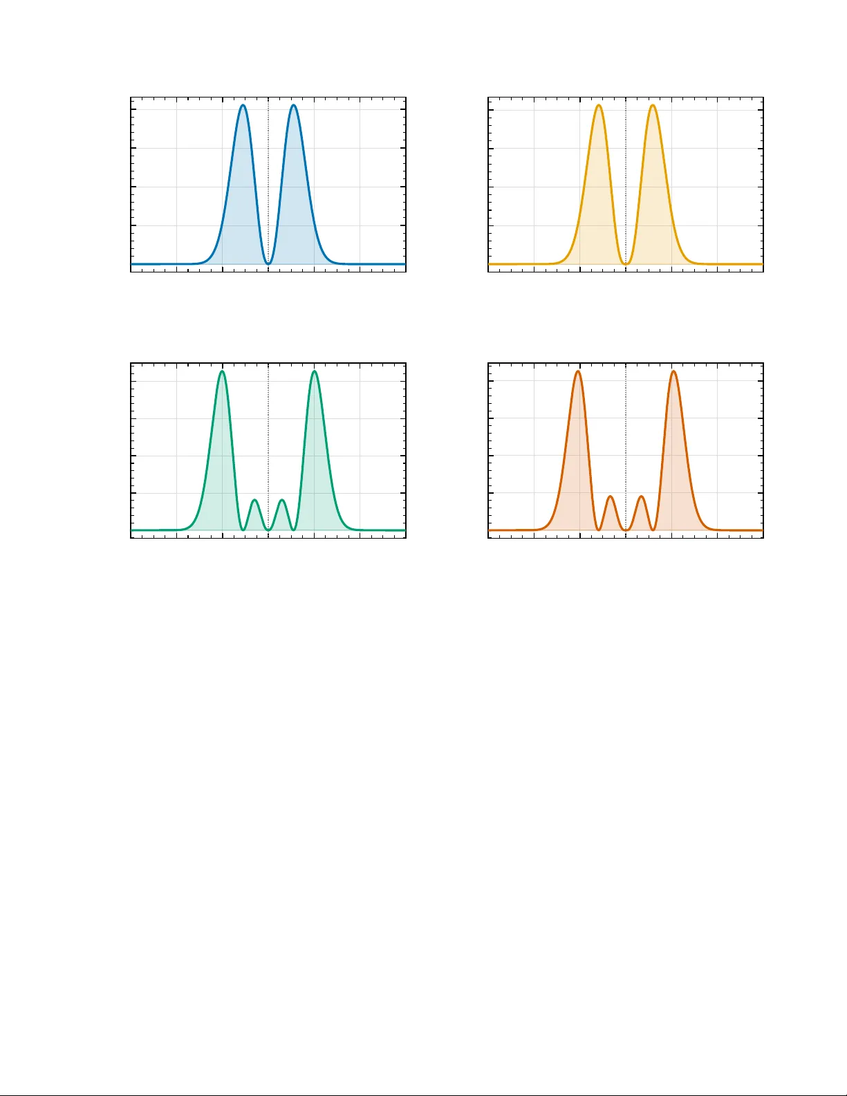
Analytical Solutions of One-Dimensional ( 1 D ) P oten tials for Spin-0 P articles via the F esh bac h-Villars F ormalism Ab delmalek Boumali , 1 , ∗ Ab delmalek Bouzenada , 1, 2 , † and Edilb erto O. Silv a 3 , ‡ 1 Echahid Cheikh L arbi T eb essi University 12001, T eb essa, Algeria 2 R ese ar ch Center of Astrophysics and Cosmolo gy, Khazar University, Baku, AZ1096, 41 Mehseti Str e et, Azerb aijan 3 Dep artamento de F ´ ısic a, Universidade F e der al do Mar anh˜ ao, 65085-580, S˜ ao Lu ´ ıs, Mar anh˜ ao, Br azil W e present a uniﬁed analytical and n umerical study of the one-dimensional F eshbac h–Villars (FV) equation for spin-0 particles in the presence of sev eral representativ e external potentials. Starting from the FV formulation of the Klein–Gordon equation, we deriv e the corresponding one-dimensional master equation and analyse its solutions for Coulom b, p o wer-exponential, Cornell, P¨ osc hl–T eller, and W oo ds–Saxon interactions. F or the singular Coulomb and Cornell cases, a Loudon-t ype cutoﬀ regularisation is implemented on the full line, allowing a mathematically con trolled treatmen t of the origin and an explicit classiﬁcation of the states by parity . The Coulom b problem exhibits the exp ected near-degenerate even–odd structure in the cutoﬀ limit, while the Cornell p oten tial com bines short-distance Coulomb b ehaviour with long-distance conﬁnement and pro duces a ﬁnite set of b ound states for ﬁxed parameters. The p o wer-exponential p oten tial with p = 1 is reduced to a Whittaker-t yp e equation and yields an in trinsically relativistic sp ectrum with no standard Sc hr¨ odinger b ound-state limit in the parameter regime considered. F or the smo oth short-range P¨ osc hl–T eller and W o o ds-Saxon potentials, the FV formalism reveals, resp ectiv ely , the eﬀects of deﬁnite parity and spatial asymmetry on the sp ectrum, wa ve functions, and particle–antiparticle mixing. In all cases, we reconstruct the full FV spinor, analyse the asso ciated charge density , and compare the relativistic b eha viour with the corresp onding non-relativistic expectations whenever suc h a limit exists. The results provide a coherent set of analytical and numerical b enc hmarks for relativistic scalar bound states in one dimension. I. INTR ODUCTION Quan tum mechanics provides the fundamental description of nature at the smallest scales [ 1 ], introducing phe- nomena such as sup erp osition and entanglemen t that hav e no classical counterpart. The Schr¨ odinger equation [ 2 ] go verns the non-relativistic evolution of the wa v e function, yielding a probabilistic description of observ ables such as p osition and momentum and encapsulating the uncertaint y inheren t in microscopic systems. This framework pla ys a decisiv e role in the understanding of atomic and molecular structure, and its implications extend to modern quantum tec hnologies, including quantum computing [ 3 ] and quantum cryptography [ 4 ]. When particles attain relativistic energies or when particle–antiparticle eﬀects become relev ant, a relativistic exten- sion of quantum mec hanics is indisp ensable. The Klein–Gordon equation [ 5 ] is the natural relativistic wa ve equation for scalar (spin-0) particles, describing b osons whose quantum state is represented by a Lorentz-scalar ﬁeld. Spin-0 particles obey Bose–Einstein statistics and, unlike spin-1 / 2 fermions [ 6 ], are not sub ject to the P auli exclusion princi- ple. Their most celebrated representativ e is the Higgs b oson [ 7 – 10 ], discov ered in 2012 at the Large Hadron Collider, whic h plays a cen tral role in the Standard Model by endo wing other elemen tary particles with mass through the Higgs mec hanism. Beyond collider physics, scalar ﬁelds also arise naturally in mo dels of dark matter [ 11 ] and in eﬀective descriptions of nuclear and hadronic interactions [ 12 ]. A recurring theme in both non-relativistic and relativistic quantum mec hanics is the study of exactly solv able or analytically tractable mo dels, which serve as b enchmarks for numerical metho ds and clarify the roles of symmetry , b oundary conditions, and asymptotic behaviour. The form of the external p oten tial strongly inﬂuences the sp ectrum, the spatial proﬁle of the wa ve function, and the structure of the corresp onding b ound states. Coulom b p oten tials, c haracterised b y an inv erse-distance dep endence, are fundamental to atomic physics and arise naturally in systems go verned b y electromagnetic interactions [ 13 , 14 ]. The Cornell p otential, whic h combines a short-range Coulom b term with long-range linear conﬁnemen t, is widely used in phenomenological descriptions of quark–antiquark bound states in quantum chromodynamics [ 15 – 19 ]. The P¨ oschl–T eller potential provides a smo oth short-range w ell with deﬁnite parit y on the full line, making it particularly useful in the study of b ound states and exactly solv able mo dels. The ∗ abdelmalek.b oumali@gmail.com † abdelmalekb ouzenada@gmail.com ‡ edilberto.silva@ufma.br (Corresp. author) 2 W oo ds–Saxon p otential, central to nuclear ph ysics, describ es a diﬀuse ﬁnite-depth interaction with an asymmetric proﬁle and realistic surface b ehaviour. P ow er-exp onential p otentials of the form V ( x ) ∝ e − ( x/x 0 ) p constitute a ﬂexible and physically motiv ated family that in terp olates b et ween the Gaussian ( p = 2) and simple exp onential ( p = 1) cases. Such p otentials arise in cosmology , where they app ear in mo dels of inﬂation and scalar-ﬁeld dynamics [ 20 , 21 ], and in condensed-matter ph ysics, where they can describ e conﬁnement in quantum dots and eﬀectiv e interactions in low-dimensional systems [ 22 , 23 ]. Their analytical tractability mak es them attractiv e in relativistic quan tum mechanics, esp ecially when one wishes to compare smo oth short-range interactions with singular or conﬁning p otentials. The F esh bach–Villars (FV) formalism [ 24 ] provides an elegant reformulation of the Klein–Gordon equation. By in tro ducing a t wo-component w a ve function, the FV approac h recasts the original second-order equation in to a system of coupled ﬁrst-order equations of Sc hr¨ odinger type. This representation facilitates the inclusion of external potentials and b oundary conditions, mak es the particle–an tiparticle structure explicit, and clariﬁes the interpretation of the conserv ed charge density . The FV framew ork has b een applied to a wide range of problems, including the harmonic oscillator [ 25 ], Coulomb- and Cornell-type interactions [ 26 , 27 ], curved space-time backgrounds [ 28 , 29 ], magnetic- ﬁeld conﬁgurations [ 30 ], and systems inv olving top ological defects and Aharonov–Bohm-t yp e eﬀects [ 31 , 32 ]. More recen t work has examined the FV equation in Lorentz-violating settings [ 33 , 34 ] and explored its connection with the F oldy–W outhuysen (FW) transformation [ 35 , 36 ]. The F oldy–W outhuysen transformation is a canonical unitary transformation that blo ck-diagonalises a relativistic Hamiltonian, thereby separating p ositiv e-energy (particle) states from negative-energy (an tiparticle) states and making the non-relativistic limit more transparent. Although originally developed for the Dirac equation, it is also applicable to the FV equation for scalar particles, where it helps clarify the physical meaning of relativistic corrections and pro vides a bridge b etw een the fully relativistic dynamics and its non-relativistic approximation [ 35 , 36 ]. Despite this extensive literature, a uniﬁed treatmen t of the one-dimensional FV equation across sev eral qualitativ ely distinct external p otentials remains useful both p edagogically and physically . In particular, it is v aluable to compare, within a single framework, singular in teractions requiring regularisation, smo oth short-range wells, conﬁning p oten- tials, and asymmetric ﬁnite-range proﬁles. The presen t work addresses this goal b y analysing the FV equation for ﬁv e represen tative cases: the Coulomb, p ow er-exp onential, Cornell, P¨ osc hl–T eller, and W o o ds–Saxon p oten tials. Dep end- ing on the p oten tial, the analysis combines exact reductions to sp ecial-function equations with cutoﬀ regularisation, matc hing conditions, or direct numerical shooting. Our main ob jectives are threefold. First, we deriv e and solv e the one-dimensional FV master equation for a repre- sen tative set of p oten tials spanning singular, short-range, conﬁning, and asymmetric regimes. Second, we reconstruct the full FV spinor in each case and analyse the corresponding particle–an tiparticle mixing and conserv ed charge densit y . Third, whenever appropriate, we compare the relativistic results with their non-relativistic coun terparts and iden tify the features that are genuinely relativistic. The pap er is organised as follows. Section I I reviews the FV formalism and derives the one-dimensional master equation. Section I I I introduces the class of applications considered in this work. Section IV presents the regularised Coulom b problem. Section V analyses the p ow er-exp onential potential with p = 1. Section VI discusses the non- relativistic limit. Section VI I is dev oted to the regularised Cornell p oten tial. Section VI I I studies the P¨ osc hl–T eller p oten tial, and Section IX treats the W oo ds–Saxon case. Finally , Section X summarises the main results and outlines p ossible extensions. I I. FESHBA CH-VILLARS FORMALISM The Klein-Gordon equation is a cornerstone of relativistic quantum mechanics for spin-0 particles, yet its second- order time deriv ative leads to conceptual and practical diﬃculties. In particular, the wa ve function do es not admit an immediate probabilistic interpretation analogous to that of the Schr¨ odinger theory , and the separation b etw een particle and antiparticle comp onents is not manifest. The F eshbac h-Villars (FV) formalism [ 37 ] addresses these issues b y introducing a t wo-component representation that recasts the Klein-Gordon equation into a Schr¨ odinger-lik e ﬁrst-order form. This formulation makes the conserv ed charge density and current more transparent, facilitates the coupling to external electromagnetic ﬁelds, and provides a natural route to the non-relativistic limit. In this section, we derive the FV equations from the Klein-Gordon equation, presen t the asso ciated Hamiltonian structure and conserv ed quantities, and obtain the one-dimensional stationary equation that serves as the starting p oin t for the exact solutions discussed in the follo wing sections. Throughout this work, natural units ℏ = c = 1 are used. 3 A. F rom the Klein-Gordon equation to the FV representation W e begin with the Klein-Gordon equation for a scalar particle of mass m in the presence of an external electrostatic p oten tial V ( x, t ),  i ∂ ∂ t − eV  2 ψ =  −∇ 2 + m 2  ψ . (1) F ollo wing Ref. [ 37 ], w e in tro duce the tw o-component wa v e function Ψ =  ψ 1 ψ 2  , (2) together with the deﬁnitions ψ = ψ 1 + ψ 2 , (3) and  i ∂ ∂ t − eV  ψ = m ( ψ 1 − ψ 2 ) . (4) The quan tities ψ 1 and ψ 2 ma y b e interpreted as the particle and an tiparticle comp onen ts of the FV wa ve function, resp ectiv ely . F or stationary states, ψ ( x, t ) = e − iE t ψ ( x ), Eqs. ( 3 ) and ( 4 ) immediately yield ψ 1 ( x ) = 1 2  1 + E − eV ( x ) m  ψ ( x ) , (5) ψ 2 ( x ) = 1 2  1 − E − eV ( x ) m  ψ ( x ) . (6) These relations make explicit how the external p oten tial mixes the tw o comp onents. B. Deriv ation of the F esh bach-Villars equations Substituting the decomp osition ( 3 ) and the auxiliary relation ( 4 ) in to the Klein-Gordon equation ( 1 ), one obtains a coupled system for the sum and diﬀerence of the FV comp onents:  i ∂ ∂ t − eV  ( ψ 1 + ψ 2 ) = m ( ψ 1 − ψ 2 ) , (7)  i ∂ ∂ t − eV  ( ψ 1 − ψ 2 ) =  ˆ p 2 m + m  ( ψ 1 + ψ 2 ) , (8) where ˆ p = − i ∇ is the momentum op erator. By taking the sum and the diﬀerence of Eqs. ( 7 ) and ( 8 ), one arrives at the F eshbac h-Villars equations for a spin-0 particle: i ∂ ψ 1 ∂ t = ˆ p 2 2 m ( ψ 1 + ψ 2 ) + ( m + eV ) ψ 1 , (9) i ∂ ψ 2 ∂ t = − ˆ p 2 2 m ( ψ 1 + ψ 2 ) − ( m − eV ) ψ 2 . (10) These t wo coupled ﬁrst-order equations are Schr¨ odinger-like in structure and constitute the basis of the FV represen- tation [ 37 ]. 4 C. Hamiltonian form and Pauli-matrix structure Equations ( 9 ) and ( 10 ) can b e written compactly as i ∂ Ψ ∂ t = H FV Ψ , (11) with Hamiltonian H FV = ( τ 3 + iτ 2 ) ˆ p 2 2 m + τ 3 m + eV , (12) where τ i ( i = 1 , 2 , 3) are the Pauli matrices, τ 1 =  0 1 1 0  , τ 2 =  0 − i i 0  , τ 3 =  1 0 0 − 1  . (13) The matrix combination ( τ 3 + iτ 2 ) takes the explicit form τ 3 + iτ 2 =  1 1 1 1  , (14) sho wing that the kinetic term couples symmetrically to b oth FV comp onen ts, as exp ected from Eqs. ( 9 ) and ( 10 ). An imp ortant prop ert y of the FV Hamiltonian is its pseudo-Hermiticity [ 36 ], H FV = τ 3 H † FV τ 3 , H † FV = τ 3 H FV τ 3 , (15) whic h guarantees the conserv ation of the τ 3 -w eighted inner pro duct and is compatible with a real energy sp ectrum under the appropriate physical boundary conditions. D. Electromagnetic interaction and conserved current In the presence of a general external electromagnetic ﬁeld describ ed by the four-p oten tial ( A 0 , A ), the minimal- coupling prescription ˆ p → ˆ p − e A leads to the FV Hamiltonian [ 37 ] H FV = ( τ 3 + iτ 2 ) ( ˆ p − e A ) 2 2 m + mτ 3 + eA 0 . (16) The asso ciated conserved c harge densit y and current are [ 32 ] ρ ( r , t ) = Ψ † τ 3 Ψ = | ψ 1 | 2 − | ψ 2 | 2 , (17) and J ( r , t ) = i 2 m  Ψ † τ 3 ( τ 3 + iτ 2 ) ∇ Ψ − ( ∇ Ψ † ) τ 3 ( τ 3 + iτ 2 )Ψ  − e m A Ψ † τ 3 ( τ 3 + iτ 2 )Ψ , (18) whic h satisfy the contin uit y equation ∂ ρ ∂ t + ∇ · J = 0 . (19) Accordingly , ρ is interpreted not as a probabilit y density in the non-relativistic sense, but as a charge density . It is p ositiv e for p ositiv e-energy solutions and negative for negative-energy solutions, thereby distinguishing particle and an tiparticle sectors. 5 E. One-dimensional stationary equation F or the one-dimensional problem c onsidered in this work, we restrict ourselves to a purely electrostatic p oten tial V ( x ) and seek stationary solutions of the form Ψ( x, t ) = e − iE t  ψ 1 ( x ) ψ 2 ( x )  , (20) where E is the energy eigenv alue. Substituting Eq. ( 20 ) into Eqs. ( 9 ) and ( 10 ), w e obtain the coupled stationary equations [ 38 ] E ψ 1 = − 1 2 m d 2 dx 2 ( ψ 1 + ψ 2 ) + mψ 1 + eV ( x ) ψ 1 , (21) E ψ 2 = + 1 2 m d 2 dx 2 ( ψ 1 + ψ 2 ) − mψ 2 + eV ( x ) ψ 2 . (22) T o decouple the system, we deﬁne the sum and diﬀerence functions ψ s = ψ 1 + ψ 2 , ψ d = ψ 1 − ψ 2 . (23) Adding Eqs. ( 21 ) and ( 22 ), one obtains E ψ s = mψ d + eV ( x ) ψ s , (24) whereas subtracting Eq. ( 22 ) from Eq. ( 21 ) yields E ψ d = − 1 m d 2 ψ s dx 2 + mψ d . (25) Equation ( 24 ) gives ψ d = E − eV ( x ) m ψ s . (26) Substituting Eq. ( 26 ) into Eq. ( 25 ), we arriv e at the master equation for ψ s , d 2 ψ s ( x ) dx 2 +  ( E − eV ( x )) 2 − m 2  ψ s ( x ) = 0 . (27) This equation has exactly the form of the one-dimensional Klein-Gordon equation with electrostatic p oten tial eV ( x ), th us conﬁrming the self-consistency of the FV formulation. Once ψ s ( x ) is known, the individual FV comp onents are reconstructed from ψ 1 ( x ) = 1 2  1 + E − eV ( x ) m  ψ s ( x ) , (28) ψ 2 ( x ) = 1 2  1 − E − eV ( x ) m  ψ s ( x ) . (29) These expressions make explicit the role of the external ﬁeld in mixing the particle and antiparticle sectors: for V = 0 and p ositive energy , ψ 1 dominates ov er ψ 2 , whereas a suﬃciently strong attractive p otential may enhance the antiparticle comp onent signiﬁcantly . Equation ( 27 ) is the fundamental equation to b e solved analytically for the external p otentials considered in the following sections. 6 I I I. APPLICA TIONS: MOTIV A TION AND OVER VIEW The exact analytical study of the FV equation for sp eciﬁc external p otentials is imp ortan t for several reasons. F rom a theoretical p ersp ectiv e, closed-form solutions provide direct insight into the interpla y b etw een re lativistic kinematics and the spatial proﬁle of the external ﬁeld, an interpla y that is absent in the non-relativistic Sc hr¨ odinger theory . Within the FV framework, this interpla y is encoded in the term ( E − eV ( x )) 2 in Eq. ( 27 ): ev en when the external p otential has a simple functional form, the resulting eﬀective relativistic dynamics is highly non-trivial. F rom a practical persp ective, exact or quasi-exact solutions provide v aluable benchmarks for n umerical, v ariational, and semiclassical metho ds. They also allow a transparen t discussion of quantum n um b ers, level ordering, degeneracy patterns, comp onen t mixing, and the non-relativistic limit. In addition, comparing several analytically tractable p oten tials within the same relativistic formalism helps clarify which sp ectral and wa v e-function features are universal and which dep end sensitively on the detailed shap e of the interaction. The p oten tials considered in this work are b oth physically relev ant and mathematically complementary . The Coulom b interaction is the prototype of a singular long-range p oten tial and, in the relativistic spin-0 con text, plays a role analogous to that of the hydrogen atom in elemen tary quantum mechanics. Conﬁning and screened interactions, suc h as the Cornell, p ow er-exp onen tial, P¨ osc hl-T eller, and W oo ds-Saxon p oten tials, prob e diﬀerent combinations of short-range structure, ﬁnite-range smo othness, and asymptotic b eha viour. T ak en together, these examples illustrate ho w qualitativ ely distinct external ﬁelds generate markedly diﬀeren t sp ectral structures within the same F esh bach- Villars framework. IV. COULOMB-TYPE POTENTIAL: CUTOFF REGULARIZA TION ` A LA LOUDON The one-dimensional Coulomb problem requires sp ecial care b ecause the p otential is singular at the origin. In the full-line form ulation, V ( x ) ∝ 1 / | x | is not a regular p oten tial in the ordinary Sturm–Liouville sense, and a direct treatmen t of the singular equation ma y obscure the status of ev en-parity states, the origin of the o dd–even degeneracy , and the meaning of the deeply lo calised state near x = 0. F or this reason, rather than solving the singular problem ab initio , we follow the regularisation strategy introduced by Loudon for the one-dimensional hydrogen atom [ 39 , 40 ]: the singularity is ﬁrst smo othed by a short-distance cutoﬀ, the b ound-state problem is solved for the regularised p oten tial, and only afterwards is the limit in which the cutoﬀ tends to zero considered. This pro cedure provides a mathematically con trolled route to the singular problem and makes transparent the physical origin of the sp ectral features that survive in the hard-core limit. W e therefore replace the singular Coulom b in teraction by the regularised even p oten tial V δ ( x ) =      a δ , | x | < δ , a | x | , | x | ≥ δ, a > 0 , (30) where δ > 0 is a small cutoﬀ length, and we deﬁne, as b efore, α ≡ ea . In the F eshbac h–Villars formalism, the sum comp onen t ψ s satisﬁes d 2 ψ s dx 2 +  ( E − eV δ ( x )) 2 − m 2  ψ s = 0 . (31) Because V δ ( x ) is ev en, the eigenstates can be classiﬁed b y parit y , in direct analogy with Loudon’s regularised treatmen t of the one-dimensional hydrogen atom [ 39 , 40 ], ψ s ( − x ) = ± ψ s ( x ) , (32) with the plus (minus) sign corresp onding to even (o dd) states. F or the exterior region | x | ≥ δ , Eq. ( 31 ) reduces to d 2 ψ s dx 2 +  α 2 x 2 − 2 E α | x | − k 2  ψ s = 0 , k 2 ≡ m 2 − E 2 > 0 , (33) whic h is the same Coulomb equation obtained from the singular problem, but now p osed only outside the regularised core. Introducing z = 2 k | x | , the deca ying solution can b e written as ψ (out) s ( x ) = C W λ,µ (2 k | x | ) , (34) 7 where W λ,µ is the Whittaker function and λ = E α k , µ = 1 2 p 1 − 4 α 2 . (35) The restriction | α | ≤ 1 / 2 is again required in order for µ to remain real and for the exterior solution to display the standard b ound-state b eha viour. Inside the core, | x | < δ , the p oten tial is constant and Eq. ( 31 ) b ecomes d 2 ψ s dx 2 + p 2 δ ψ s = 0 , p 2 δ =  E − α δ  2 − m 2 . (36) F or the parameter range of in terest and suﬃciently small δ , one has p 2 δ > 0, and the regular interior solutions are ψ (in , even) s ( x ) = A cos( p δ x ) , ψ (in , odd) s ( x ) = B sin( p δ x ) . (37) The sp ectrum is determined by matching ψ s and dψ s /dx at x = δ . Deﬁning the logarithmic deriv ativ e of the exterior solution by L ( E , δ ) ≡ d dx ln ψ (out) s ( x )     x = δ + , (38) the matching conditions b ecome L ( E , δ ) = − p δ tan( p δ δ ) (ev en states) , (39) L ( E , δ ) = p δ cot( p δ δ ) (o dd states) . (40) Equations ( 39 ) and ( 40 ) therefore provide the regularised quantisation conditions for the full one-dimensional problem. The structure of the b ound-state sp ectrum that emerges from these quantisation conditions is illustrated in Fig. 1 . The left panel shows the particle eigen v alues E part n /m as a function of the quan tum n umber n for three v alues of the coupling constan t, α = 0 . 10, 0 . 25, and 0 . 45, with the cutoﬀ ﬁxed at δ = 0 . 05 m − 1 . All levels lie inside the mass gap, 0 < E part n < m , and accumulate monotonically tow ard the contin uum threshold E = m as n increases, repro ducing the Rydb erg-lik e compression of the sp ectrum at large n . The stronger the coupling, the more deeply the ground state is pulled aw ay from the threshold. The right panel displays the antiparticle counterpart E anti n /m , obtained from the particle sp ectrum through the charge-conjugation symmetry of the FV equation: the simultaneous substitutions E → − E and α → − α lea ve Eq. ( 31 ) inv arian t, so that E anti n = − E part n , with all levels in the range − m < E anti n < 0. T o complemen t the sp ectral information, it is useful to examine the spatial structure of the corresp onding Coulomb eigenfunctions. This is illustrated in Fig. 2 , which displays the normalised wa ve functions ψ n ( x ) for the four low est states, n = 0 , 1 , 2 , 3, at ﬁxed coupling α = 0 . 20. As exp ected, the ground state is no deless and strongly concen trated near the origin, while the excited states develop an increasing num b er of no des and extend ov er progressively larger spatial regions. This b ehaviour reﬂects the usual hierarch y of b ound states in an attractive Coulomb-lik e in teraction: higher v alues of n corresp ond to less tightly b ound states, with broader spatial supp ort and a more pronounced oscillatory structure b efore the asymptotic decay sets in. When all proﬁles are sho wn on the same axis, one clearly sees the combined eﬀect of the increasing radial extent and the growing num b er of oscillations as the excitation level rises. The corresp onding probabilit y densities are shown in Fig. 3 for the same v alue α = 0 . 20. The ground-state density is sharply localised near the origin and decreases monotonically with x , whereas the excited-state densities b ecome progressiv ely broader and develop the exp ected internal structure asso ciated with the no des of the wa v e functions. In particular, the num b er of lo cal maxima increases with n , and the dominant supp ort of the distribution is displaced to ward larger v alues of x , indicating that the higher states are more spatially extended. T aken together, these panels pro vide a complementary visualisation of the b ound-state hierarc h y: while the w av e functions exhibit alternating signs and no des, the densities emphasise the out ward spreading and increasing spatial complexity of the excited Coulom b states. This regularised form ulation clariﬁes several p oints that remain hidden in the strictly singular treatment. First, o dd states are unproblematic: because ψ s (0) = 0, they are naturally protected from the core singularity and, in the limit δ → 0 + , they approach the usual Coulombic Balmer-type sequence. Second, even states are also p erfectly well deﬁned at ﬁnite δ , but their existence is controlled b y the matching condition ( 39 ); when the cutoﬀ is sent to zero, the regularised even levels collapse onto the o dd ones, thereby explaining the well-kno wn pairwise o dd–ev en degeneracy 8 0 3 6 9 12 15 18 21 n 0 . 850 0 . 875 0 . 900 0 . 925 0 . 950 0 . 975 1 . 000 E n / m (a) Particle ( E part n ) α = 0 . 1 α = 0 . 25 α = 0 . 45 0 3 6 9 12 15 18 21 n − 1 . 000 − 0 . 975 − 0 . 950 − 0 . 925 − 0 . 900 − 0 . 875 − 0 . 850 E n / m (b) Antiparticle  E anti n  Energy levels — Coulomb p otential (Loudon cutoﬀ, δ = 0 . 05) FIG. 1. Bound-state energy sp ectrum of the regularised one-dimensional Coulomb p oten tial in the F esh bach–Villars formalism, for δ = 0 . 05 m − 1 and three v alues of the coupling constant α . L eft p anel : particle eigenv alues E part n /m as a function of the principal quantum num b er n . Right p anel : antiparticle eigenv alues E anti n /m = − E part n , obtained from the charge-conjugation symmetry E → − E , α → − α of Eq. ( 31 ). All lev els lie inside the mass gap, | E n | < m , and accumulate tow ard | E | = m as n increases. Deeply lo calised states (Loudon core states) are excluded from b oth panels, since they are artefacts of the ﬁnite cutoﬀ and disapp ear in the limit δ → 0 + (see text). 0 50 100 150 200 250 x − 0 . 2 − 0 . 1 0 . 0 0 . 1 0 . 2 0 . 3 0 . 4 ψ n ( x ) (normalised) n = 0 n = 1 n = 2 n = 3 FIG. 2. Normalised Coulomb wa ve functions ψ n ( x ) for the one-dimensional problem, with α = 0 . 20 and m = 1, shown for the four low est states n = 0 , 1 , 2 , 3. Each curve is plotted ov er a suﬃciently large interv al to capture b oth its oscillatory structure and asymptotic decay , and all of them are display ed together on a common axis for direct comparison. As n increases, the w av e functions extend ov er progressively larger spatial regions and develop the exp ected increase in the num b er of no des, while their amplitudes b ecome more spread out ov er the classically allow ed region. of the one-dimensional Coulomb problem in the cutoﬀ limit, exactly as in Loudon’s construction [ 39 , 40 ]. Third, the regularised problem contains an additional deeply lo calised even state whose probability densit y b ecomes increasingly concen trated inside the core as δ decreases. In Loudon’s non-relativistic analysis, its binding energy diverges as δ → 0 + [ 39 , 40 ]; in the present relativistic FV setting, the same tendency indicates that the state is driv en b eyond the regime in which a single-particle interpretation can b e trusted. F or this reason, in what follows we fo cus on the regular b ound-state branch contin uously connected to the ﬁnite-gap sector | E | < m . The cutoﬀ construction th us pro vides the appropriate mathematical foundation for the Coulomb problem in one 9 0 10 20 30 40 50 x 0 . 00 0 . 05 0 . 10 0 . 15 | ψ n ( x ) | 2 (a) n = 0 , α = 0 . 20 (1 p eak) 0 25 50 75 100 125 x 0 . 00 0 . 02 0 . 04 0 . 06 | ψ n ( x ) | 2 (b) n = 1 , α = 0 . 20 (2 p eaks) 0 50 100 150 200 250 x 0 . 00 0 . 02 0 . 04 | ψ n ( x ) | 2 (c) n = 2 , α = 0 . 20 (3 p eaks) 0 100 200 300 x 0 . 00 0 . 01 0 . 02 0 . 03 | ψ n ( x ) | 2 (d) n = 3 , α = 0 . 20 (4 p eaks) FIG. 3. Probabilit y densities | ψ n ( x ) | 2 for the one-dimensional Coulomb problem with α = 0 . 20 and m = 1, for the four low est states: (a) n = 0, (b) n = 1, (c) n = 2, and (d) n = 3. Each panel is display ed ov er an adaptive spatial interv al c hosen to mak e the full proﬁle visible. The densities b ecome progressively broader as n increases and exhibit the corresp onding increase in radial structure, with the num ber of lo cal maxima gro wing from the ground state to the excited states. This b ehaviour reﬂects the increasingly extended character of the higher Coulomb eigenstates. dimension. The singular equation is not taken as the starting point, but rather as the limiting form of a family of regular problems [ 39 , 40 ]. This has tw o imp ortant consequences for the presen t work. On the one hand, it justiﬁes the use of parit y as a go o d quan tum num b er in the full-line problem and explains the emergence of o dd–even degeneracy in the hard-core limit. On the other hand, it shows that the near-origin b ehaviour of the FV spinor comp onents m ust b e in terpreted through a limiting procedure rather than b y assigning an independent ph ysical meaning to the formally singular p oint x = 0. Once the regularised eigen v alue E n, ± ( δ ) is obtained from Eqs. ( 39 ) and ( 40 ), the FV spinor components are reconstructed from Eqs. ( 28 ) and ( 29 ): ψ 1 ( x ) = 1 2  1 + E − eV δ ( x ) m  ψ s ( x ) , ψ 2 ( x ) = 1 2  1 − E − eV δ ( x ) m  ψ s ( x ) . (41) Ph ysical densities and observ ables are then computed at ﬁnite δ and only afterwards examined in the limit δ → 0 + . The internal structure of the FV s pinor for the regularised Coulomb p otential is sho wn in Fig. 4 , for α = 0 . 20 and δ = 0 . 05 m − 1 . The left (right) panel corresp onds to the low est o dd (even) state. In b oth cases the sum comp onent ψ s (solid blue) is a smo oth function that joins the oscillatory interior solution across | x | = δ (marked by vertical dashed lines) to the monotonically decaying Whittaker exterior. The particle comp onen t ψ 1 (red dashed) dominates in magnitude throughout the domain, while the an tiparticle comp onent ψ 2 (green dotted) remains smaller but non-zero and enco des the relativistic correction to the non-relativistic limit. Its spatial proﬁle mirrors that of ψ 1 , mo dulated b y the lo cal v alue of the p otential through the factor [1 − ( E − eV δ ) /m ]; the enhancement near the origin visible inside 10 the core reﬂects the large v alue of eV δ = α/δ in that region. − 10 − 5 0 5 10 x − 0 . 2 − 0 . 1 0 . 0 0 . 1 0 . 2 Amplitude (a) Odd state, α = 0 . 2, δ = 0 . 05, E /m = 0 . 9789 ψ s = ψ 1 + ψ 2 ψ 1 (part ´ ıcula) ψ 2 (antipart ´ ıcula) − 10 − 5 0 5 10 x 0 . 00 0 . 05 0 . 10 0 . 15 0 . 20 0 . 25 Amplitude (b) Even state, α = 0 . 2, δ = 0 . 05, E /m = 0 . 9799 FIG. 4. F eshbac h–Villars spinor components for the regularised Coulomb potential with α = 0 . 20 and δ = 0 . 05 m − 1 . (a) low est o dd-parit y state ( n = 0, o dd). (b) low est even-parit y state ( n = 0, even). Solid blue: sum comp onent ψ s = ψ 1 + ψ 2 . Dashed red: particle comp onent ψ 1 . Dotted green: antiparticle component ψ 2 . The v ertical dotted grey lines mark the cutoﬀ b oundary x = ± δ , across which the interior oscillatory solution is matched to the exterior Whittaker function. The particle comp onen t dominates throughout, while ψ 2 acquires a visible enhancement inside the core owing to the large constan t p otential eV δ = α/δ . A quantitativ e measure of the relativistic conten t of each state is pro vided by the ratio | ψ 2 /ψ 1 | , plotted in Fig. 5 for the low est o dd state and three v alues of α . In the exterior region x > δ , where eV δ ( x ) = α/x , this ratio takes the explicit form     ψ 2 ψ 1     =     1 − ( E − α/x ) /m 1 + ( E − α/x ) /m     , (42) whic h is a monotonically decreasing function of x for ﬁxed E and α in the parameter range considered here. At large distances, where α/x ≪ E , it approaches the constant non-relativistic limit ( m − E ) / ( m + E ) in magnitude, so the ratio is suppressed whenever the binding energy m − E is small. Near the cutoﬀ, by contrast, the growing p otential ampliﬁes ψ 2 and the ratio increases. The ﬁgure conﬁrms all three trends: for larger α the ratio is higher at every x (stronger coupling implies stronger relativistic eﬀects), it increases noticeably as x → δ + , and it settles to a nearly constan t v alue at large x . Finally , Fig. 6 compares the FV c harge density ρ = | ψ 1 | 2 − | ψ 2 | 2 with the squared sum comp onent | ψ s | 2 for the same parameters as Fig. 4 . The tw o quantities agree closely in the exterior region, where the relativistic correction enco ded in ψ 2 is small, but diﬀer visibly inside the core: the large constan t v alue eV δ = α /δ enhances the lo cal comp onen t mixing and pro duces a noticeable separation b etw een ρ and | ψ s | 2 for | x | < δ . Crucially , ρ remains non-negative for the p ositive-energy gap states considered here and satisﬁes the FV normalisation condition R + ∞ −∞ ρ dx = 1, conﬁrming the consistency of the single-particle charge-densit y interpretation within the gap sector. In numerical practice, one may solve the regularised problem for a sequence of decreasing cutoﬀs δ , verify the con vergence of the o dd and ev en excited levels tow ard common limiting v alues, and monitor separately the collapse of the deeply lo calised even branc h. This strategy remov es the mathematical ambiguit y at the origin and yields a clearer ph ysical in terpretation of the relativistic one-dimensional Coulom b problem within the F esh bac h–Villars formalism. V. PO WER-EXPONENTIAL POTENTIAL ( p = 1 ) The p ow er-exp onential p otential b elongs to a physically distinct class from the Coulomb interaction: whereas the Coulom b p oten tial is long-ranged and singular at the origin, the exp onential p otential is short-ranged and b ounded ev erywhere. This complementary c haracter makes it a useful counterpart to the Coulomb case. W e consider the general p ow er-exponential form [ 20 – 23 ] V p ( x ) = − V 0 exp  −  x x 0  p  , V 0 > 0 , p ≥ 1 , (43) 11 0 2 4 6 8 10 12 14 x 0 . 0 0 . 2 0 . 4 0 . 6 0 . 8 | ψ 2 /ψ 1 | An tiparticle-to-particle ratio (o dd state, Loudon cutoﬀ ) α = 0 . 25 α = 0 . 45 FIG. 5. Ratio | ψ 2 /ψ 1 | of the antiparticle to particle comp onents as a function of x > 0, for the low est o dd state with δ = 0 . 05 m − 1 and three v alues of the coupling constant α . The vertical dotted line marks the cutoﬀ radius x = δ . F or x > δ the ratio is given analytically by Eq. ( 42 ) and decreases monotonically from a maximum at the cutoﬀ b oundary tow ard the asymptotic v alue ( m − E 0 ) / ( m + E 0 ) in magnitude at large x . Larger coupling pro duces a uniformly higher ratio, reﬂecting the increasing relativistic character of the more deeply b ound states. − 15 − 10 − 5 0 5 10 15 x 0 . 00 0 . 01 0 . 02 0 . 03 0 . 04 0 . 05 0 . 06 Densidade (a) Odd state, α = 0 . 2, δ = 0 . 05 | ψ s | 2 ρ = | ψ 1 | 2 − | ψ 2 | 2 − 15 − 10 − 5 0 5 10 15 x 0 . 00 0 . 01 0 . 02 0 . 03 0 . 04 0 . 05 0 . 06 Densidade (b) Even state, α = 0 . 2, δ = 0 . 05 FIG. 6. Comparison of the FV charge density ρ = | ψ 1 | 2 − | ψ 2 | 2 (dashed red) and the squared sum comp onent | ψ s | 2 (solid blue) for α = 0 . 20 and δ = 0 . 05 m − 1 . (a) low est o dd-parity state. (b) low est even-parit y state. V ertical dotted grey lines indicate the cutoﬀ b oundary x = ± δ . In the exterior region, the tw o curves nearly coincide, since the antiparticle amplitude is small there. Inside the core the constant p otential eV δ = α/δ pro duces a visible separation b etw een ρ and | ψ s | 2 . The density ρ is non-negative throughout and satisﬁes the FV normalisation R ρ dx = 1, conﬁrming the consistency of the one-particle in terpretation within the mass gap. and fo cus here on p = 1, which yields a simple decaying exponential and admits an exact reduction to Whittaker functions. With the shorthands b ≡ eV 0 and q ≡ x 0 , the p otential b ecomes eV ( x ) = − b e − x/q . (44) 12 F or deﬁniteness, we work on the half-line x ≥ 0. The master equation ( 27 ) then b ecomes d 2 ψ s dx 2 + h b 2 e − 2 x/q + 2 bE e − x/q + κ 2 i ψ s = 0 , (45) where κ 2 ≡ E 2 − m 2 . (46) T o reduce Eq. ( 45 ) to standard form, we ﬁrst set ψ s ( x ) = e x/ (2 q ) D ( x ) , (47) and then introduce the change of v ariable z = 2 ibq e − x/q , (48) whic h maps x ∈ (0 , ∞ ) onto a curve in the complex z -plane. Under these substitutions, Eq. ( 45 ) transforms in to the Whittak er equation [ 41 ] d 2 D dz 2 +  − 1 4 + µ W z + 1 − 4 ν 2 W 4 z 2  D = 0 , (49) with parameters µ W = − iE q , ν W = iq κ. (50) The tw o indep enden t solutions are the Whittaker functions M µ W ,ν W ( z ) and W µ W ,ν W ( z ). As x → ∞ , one has z → 0, and the behaviour of W µ W ,ν W ( z ) near z = 0 yields a div ergent con tribution. Requiring the physical solution to remain ﬁnite as x → ∞ therefore eliminates that branch. Using the connection b et ween the Whittaker M function and the conﬂuen t h yp ergeometric function 1 F 1 ( a, b, z ) [ 41 ], the resulting solution ma y b e written as ψ s ( x ) = N n e x/ (2 q )  2 ibq e − x/q  1 2 + iq κ exp  − ibq e − x/q  1 F 1  1 2 + iE q + iq κ, 1 + 2 iq κ, 2 ibq e − x/q  , (51) where N n is a normalisation constant to b e interpreted in a b ox-normalisation sense, or else ov er a ﬁnite plotting in terv al, since the states discussed b elow are not square-integrable in the usual sense. F or large | z | , the conﬂuent hypergeometric function 1 F 1 ( a, b, z ) grows exp onentially unless the series terminates. T ermination o ccurs when 1 2 + iE q + iq κ = − n, n = 0 , 1 , 2 , . . . , (52) whic h yields the quantisation condition. Using κ 2 = E 2 − m 2 , one obtains the corresp onding sp ectrum E n = ± m 2 q 2 +   n + 1 2   2 2 q   n + 1 2   . (53) The ± sign corresp onds to the particle and antiparticle branches. The c haracteristic half-integer shift   n + 1 2   is a direct consequence of the Whittaker parameters and has no counterpart in the Coulomb sp ectrum. F or large n , the energy grows approximately linearly , E n ≈ | n + 1 2 | 2 q , (54) whereas for ﬁxed n the lev els decrease as q increases. As written, Eq. ( 53 ) depends on m , q , and n , while the parameter b aﬀects the local spatial structure of the w av e function through the argument of the h yp ergeometric function and the FV comp onent mixing, rather than the discrete energies themselv es. The energy levels E n are display ed in Fig. 7 for three v alues of q . F or small q (a narrow er eﬀective in teraction region) the levels are more widely spaced; as q increases, the p otential broadens and the levels decrease. In all cases the levels grow with n , and the gro wth is faster for smaller q . 13 0 1 2 3 4 5 6 7 n 2 4 6 E n / m Energy levels — p o wer-exponential ( p = 1 ) q = 0 . 5 q = 1 . 0 q = 2 . 0 FIG. 7. Energy levels E n (particle branch) as a function of the quantum num ber n for the p ow er-exp onential p otential ( p = 1, m = 1) and q = 0 . 5 (circles), q = 1 . 0 (squares), and q = 2 . 0 (triangles). The lev els gro w appro ximately linearly with n for large n , in contrast to the Coulomb case. Smaller q corresp onds to a narrow er interaction region and larger lev el spacings. The complete t wo-component FV w av e function is reconstructed by inserting ψ s ( x ) into Eqs. ( 28 ) and ( 29 ) with eV ( x ) = − b e − x/q : Ψ total ( x ) = N n 2    1 + 1 m  E + b e − x/q  1 − 1 m  E + b e − x/q     e x/ (2 q )  2 ibq e − x/q  1 2 + iq κ e − ibq e − x/q × 1 F 1  1 2 + iE q + iq κ, 1 + 2 iq κ, 2 ibq e − x/q  , (55) where N n is ﬁxed by the chosen b ox normalisation or b y n umerical normalisation ov er the display ed interv al. The t wo-component spinor structure reﬂects the interpla y b etw een the energy E , the rest mass m , and the lo cal v alue of the p oten tial b e − x/q : where the p oten tial is stronger, the tw o components are more strongly mixed, while far from the source the mixing approaches the constant v alue set by E /m . The tw o-comp onen t structure of the FV spinor for the p ow er-exponential p otential diﬀers qualitatively from the Coulom b case and therefore deserves separate discussion. A key p oin t follows immediately from Eq. ( 53 ): for the particle branch one has E n > m for all n , so κ = p E 2 − m 2 (56) is real and p ositive. Accordingly , ψ s oscillates asymptotically rather than decaying exp onentially . The corresp onding stationary s tates are therefore delta-normalisable rather than L 2 -normalisable, and the proﬁles sho wn b elow should b e understo o d in a b o x-normalisation sense or as numerically normalised ov er a ﬁnite plotting window. The individual comp onents ψ 1 and ψ 2 , reconstructed from Eqs. ( 28 ) and ( 29 ) with eV ( x ) = − b e − x/q , are display ed in Fig. 8 for n = 0 and n = 1 with b = 2 and q = 1. The particle comp onent ψ 1 dominates ov er ψ 2 throughout the domain, as exp ected for a p ositiv e-energy state, but the antiparticle comp onent is appreciably larger near the origin than at large x . This spatial dependence is controlled by the local mixing factor ( E + b e − x/q ) /m : at the origin it tak es the v alue ( E + b ) /m , reﬂecting the full depth of the p otential well, and it decreases monotonically to E /m as x → ∞ , where the p otential v anishes. Unlike the Coulomb case, where the mixing div erges at the origin b ecause of the 1 /x singularit y , here the mixing remains b ounded everywhere and approaches a ﬁnite asymptotic v alue determined by E /m . The dep endence of the particle–an tiparticle mixing on the p otential depth is shown in Fig. 9 , which displays the ratio | ψ 2 /ψ 1 | for the ground state and three v alues of b . In all cases the ratio decreases monotonically from a maximum at x = 0 to the asymptotic v alue     1 − E /m 1 + E /m     (57) 14 0 2 4 6 8 10 x 0 . 0 0 . 2 0 . 4 0 . 6 0 . 8 1 . 0 En velope amplitude n = 0, b = 2 . 0, q = 1 . 0, E 0 /m = 1 . 2500 | ˜ φ s | (env elope) | ˜ ψ 1 | (particle) | ˜ ψ 2 | (antiparticle) 0 2 4 6 8 10 x 0 . 0 0 . 2 0 . 4 0 . 6 0 . 8 1 . 0 En velope amplitude n = 1, b = 2 . 0, q = 1 . 0, E 1 /m = 1 . 0833 | ˜ φ s | (env elope) | ˜ ψ 1 | (particle) | ˜ ψ 2 | (antiparticle) FIG. 8. Real parts of the FV spinor components ψ 1 (particle, red dashed), ψ 2 (an tiparticle, green dotted), and the sum function ψ s = ψ 1 + ψ 2 (blue solid) for the p o wer-exponential p oten tial ( p = 1) with b = eV 0 = 2, q = 1, and m = 1. Left panel: n = 0, E 0 /m = 1 . 2500. Right panel: n = 1, E 1 /m = 1 . 0833. The wa ve functions are oscillatory throughout the domain b ecause E n > m for all n , so κ = √ E 2 − m 2 is real. The display ed proﬁles are normalised numerically ov er the plotted interv al. The an tiparticle comp onen t ψ 2 is largest near the origin, where the p oten tial is deepest, and approaches a ﬁnite non-zero asymptotic amplitude ratio relative to ψ 1 as x → ∞ . as x → ∞ , reﬂecting the approach of the lo cal mixing factor to its free-ﬁeld limit. The spatial proﬁle is smo oth and monotonic, without the sharp near-origin divergence characteristic of the Coulom b case. Since Eq. ( 53 ) is independent of b , the asymptotic plateau is the same for ﬁxed q and n ; changing b aﬀects only the near-origin part of the curve, where the lo cal p otential still contribu tes appreciably to the FV mixing. 0 2 4 6 8 10 x 0 . 0 0 . 2 0 . 4 0 . 6 | ψ 2 /ψ 1 | P ow er-exponential ( n = 0, q = 1 . 0, m = 1) b = 1 . 0 ( | ψ 2 /ψ 1 | ∞ = 0 . 111) b = 2 . 0 ( | ψ 2 /ψ 1 | ∞ = 0 . 111) b = 3 . 0 ( | ψ 2 /ψ 1 | ∞ = 0 . 111) FIG. 9. Spatial proﬁle of the antiparticle-to-particle ratio | ψ 2 /ψ 1 | for the ground state ( n = 0, q = 1) of the p ow er-exp onential p oten tial and three v alues of the p oten tial depth: b = 1 . 0 (blue solid), b = 2 . 0 (orange dashed), and b = 3 . 0 (red dotted). In all cases the ratio decreases monotonically from a maximum at x = 0, where the p otential reaches its full depth, to the common asymptotic plateau | (1 − E /m ) / (1 + E /m ) | at large x . Increasing b enhances the near-origin mixing, while leaving the asymptotic plateau unchanged for ﬁxed q and n . This b ehaviour contrasts sharply with the Coulomb case, where the ratio div erges near the origin and v anishes asymptotically . A further consequence of the non-v anishing asymptotic mixing is visible in Fig. 10 , which compares | ψ s | 2 with the conserv ed FV charge density ρ = | ψ 1 | 2 − | ψ 2 | 2 for n = 0 and n = 1. Both quantities display oscillatory b eha viour and approac h non-zero asymptotic env elop es ov er the plotted interv al, consistent with the delta-normalisable character of the states. F or the parameter range shown, ρ lies systematically ab o ve | ψ s | 2 , reﬂecting the dominance of the particle comp onen t ov er the antiparticle comp onen t throughout the domain. The diﬀerence b etw een the tw o densities is largest where the p oten tial is deep est and the lo cal mixing is strongest. 15 0 2 4 6 8 10 x 0 1 2 3 4 ρ / | φ s | 2 = f ( x ) n = 0, q = 1 . 0, m = 1 b = 1 . 0 b = 2 . 0 b = 3 . 0 f = 1 (NR limit) 0 2 4 6 8 10 x 0 1 2 3 4 ρ / | φ s | 2 = f ( x ) n = 1, q = 1 . 0, m = 1 b = 1 . 0 b = 2 . 0 b = 3 . 0 f = 1 (NR limit) FIG. 10. Comparison b et ween the squared sum comp onent | ψ s | 2 (blue solid) and the conserved FV charge density ρ = | ψ 1 | 2 − | ψ 2 | 2 (red dashed) for the p ow er-exp onential p otential with b = 2, q = 1, and m = 1. Left panel: n = 0. Right panel: n = 1. Both quantities are computed from the n umerically normalised proﬁles o ver the displa yed in terv al and remain oscillatory at large x , consistent with the delta-normalisable character of the states. F or the parameters shown, the conserved density ρ lies ab ov e | ψ s | 2 throughout the domain b ecause the particle comp onen t remains dominant at all x . VI. NON-RELA TIVISTIC LIMIT A fundamental consistency requirement for any relativistic quantum-mec hanical framework is that it should re- duce to the corresp onding non-relativistic theory in the appropriate limit. F or the FV equation, it is conv enien t to parameterise the energy as E = m + ε m , | ε | ≪ m 2 , (58) where ε plays the role of the non-relativistic binding energy . One then expands the relev ant sp ectral formulas in in verse p o wers of m . F or the Coulomb case, k = p m 2 − E 2 ≈ √ − 2 ε (59) to leading order. Substituting E = m + ε/m into the Coulomb quantisation condition and expanding for large m , the binding energy satisﬁes ε n ≈ − α 2 m 2  n + 1 2 + 1 2 √ 1 − 4 α 2  2 . (60) F or weak coupling, α ≪ 1, one has √ 1 − 4 α 2 ≈ 1 − 2 α 2 , and Eq. ( 60 ) reduces to ε n ≈ − α 2 m 2( n + 1) 2  1 + O ( α 2 )  , (61) whic h is precisely the hydrogen-lik e Bohr formula with principal quan tum num ber N = n + 1. This pro vides a non-trivial consistency chec k of the FV formalism: the relativistic Klein–Gordon equation, solved through the FV represen tation, reproduces the correct non-relativistic limit without any additional ad ho c assumption. It is also w orth noting that the eﬀective principal quantum num b er in the relativistic treatment, n + 1 2 + 1 2 p 1 − 4 α 2 , (62) is not, in general, an integer. This fractional shift is a purely relativistic eﬀect and disapp ears as α → 0, where the standard Bohr sequence is recov ered. 16 The conv ergence of the relativistic result to its non-relativistic limit is illustrated in Fig. 11 , which shows the ground-state energy E 0 /m as a function of the mass m for three v alues of α . F or small m (strongly relativistic regime), the tw o results diﬀer appreciably , but they con verge rapidly as m increases, and for m ≳ 10 they are essen tially indistinguishable. The con vergence is faster for smaller α b ecause the relativistic correction to the binding energy is controlled by the ratio α 2 /m 2 : for small α this ratio is already negligible at mo derate m , whereas for α = 0 . 40 the corrections remain p erceptible ov er a wider range. 0 10 20 30 40 50 m 0 . 90 0 . 92 0 . 94 0 . 96 0 . 98 1 . 00 E 0 / m Non-relativistic limit ( n = 0 , Coulomb) Rel. α = 0 . 1 NR α = 0 . 1 Rel. α = 0 . 2 NR α = 0 . 2 Rel. α = 0 . 4 NR α = 0 . 4 FIG. 11. Non-relativistic limit of the ground-state ( n = 0) Coulomb energy as a function of the mass m , for α = 0 . 10 (blue), 0 . 20 (orange), and 0 . 40 (green). Solid lines: exact relativistic FV result E 0 /m . Dotted lines: non-relativistic approximation E NR /m = 1 − α 2 / (2 m ( n + 1) 2 ). The tw o curves conv erge for large m ; conv ergence is faster for smaller α . F or the p ow er-exp onential case, the non-relativistic limit is more subtle. Using Eq. ( 53 ) and expanding for large m , one ﬁnds that the corresp onding energies remain ab ov e the mass threshold, so that the stationary states discussed in Sec. V do not reduce to conv entional Sc hr¨ odinger b ound states. Equiv alently , b ecause κ 2 = E 2 − m 2 remains p ositiv e, the asymptotic b ehaviour is oscillatory rather than exp onentially decaying, and the solutions are delta-normalisable rather than square-integrable. In this sense, the p = 1 family treated here is intrinsically relativistic: a standard Sc hr¨ odinger b ound-state limit is not reco vered unless a diﬀerent scaling of the p oten tial parameters is introduced. The contrast with the Coulom b case is therefore instructive. Whereas the Coulomb sp ectrum connects smo othly to the hydrogenic Schr¨ odinger result in the weak-coupling and large-mass regime, the p o wer-exponential mo del consid- ered here does not p ossess a standard non-relativistic b ound-state counterpart in the same parameter scaling. The FV treatmen t thus rev eals an imp ortan t structural diﬀerence b etw een the tw o cases: the Coulomb branch admits a con- v entional non-relativistic interpretation, while the exp onential branch, in the form analysed here, remains essentially relativistic. VI I. CORNELL POTENTIAL The Cornell p otential combines a short-range Coulomb term with a long-range linear conﬁning term and plays a standard phenomenological role in the description of quark–antiquark bound states. In the full-line formulation, ho wev er, the one-dimensional Coulombic part of the interaction, V ( x ) ∝ 1 / | x | , is singular at the origin. T o treat this diﬃcult y in a mathematically controlled wa y and to make the parit y structure of the sp ectrum explicit, w e follow the same Loudon-t yp e regularisation strategy adopted in Section IV [ 39 , 40 ]. W e therefore replace the singular Cornell in teraction b y the regularised even p oten tial V C ,δ ( x ) =      a δ + bδ, | x | < δ, a | x | + b | x | , | x | ≥ δ, a > 0 , b > 0 , (63) where a is the Coulomb coupling, b is the string tension, and δ > 0 is a small cutoﬀ length. Deﬁning, as b efore, α ≡ ea and β ≡ eb , the FV master equation ( 27 ) b ecomes d 2 ψ s dx 2 + h  E − eV C ,δ ( x )  2 − m 2 i ψ s = 0 . (64) 17 Because V C ,δ ( x ) is even, the eigenstates can b e classiﬁed by parity , ψ s ( − x ) = ± ψ s ( x ) , (65) with the plus (minus) sign corresp onding to even (o dd) states. A. In terior Region ( | x | < δ ) Inside the regularised core the p otential is constant and Eq. ( 64 ) reduces to d 2 ψ s dx 2 + p 2 δ ψ s = 0 , p 2 δ =  E − α δ − β δ  2 − m 2 . (66) F or suﬃciently small δ , the Coulomb term α/δ dominates, so that p 2 δ > 0, and the regular interior solutions classiﬁed b y parit y are ψ (in , even) s ( x ) = A cos( p δ x ) , ψ (in , odd) s ( x ) = B sin( p δ x ) , (67) where A and B are constants ﬁxed by contin uit y at x = δ . When p 2 δ < 0, the trigonometric functions are replaced by their hyperb olic counterparts; the matching conditions b elow accommo date b oth cases in a uniﬁed wa y . B. Exterior Region ( | x | ≥ δ ) In the exterior region, the master equation tak es the form d 2 ψ s dx 2 + "  E − α | x | − β | x |  2 − m 2 # ψ s = 0 . (68) W e factor out the asymptotic b eha viour by writing ψ s ( x ) = | x | ˜ µ +1 / 2 e − β x 2 / 2 χ ( x ) , ˜ µ = 1 2 p 1 − 4 α 2 , (69) and deﬁne µ ≡ 1 2 + ˜ µ. (70) In tro ducing the v ariable ξ = √ 2 β | x | , the equation for χ is transformed into Kummer’s conﬂuent hypergeometric equation. Since the singular p oint x = 0 is excluded from the exterior region, neither indep endent solution needs to b e discarded on regularity grounds. The general exterior solution therefore reads ψ (out) s ( x ) = | x | ˜ µ +1 / 2 e − β x 2 / 2  C 1 M  a K , b K , β x 2  + C 2 U  a K , b K , β x 2  , (71) where M and U are the conﬂuent hypergeometric functions of the ﬁrst and second kind, resp ectively , and a K = µ + 1 2 + m 2 − E 2 4 β − E α √ 2 β , b K = ˜ µ + 1 2 . (72) a. Normalisability. F or large z = β x 2 , the Kummer function satisﬁes M ( a, b, z ) ∼ e z z a − b and therefore grows exp onen tially , so square-in tegrability requires C 1 = 0. By contrast, the T ricomi function b ehav es as U ( a, b, z ) ∼ z − a for large z ; an y resulting p olynomial factor is absorb ed by the Gaussian env elop e e − β x 2 / 2 , leaving a normalisable b ound-state solution throughout the parameter range of interest. The physical exterior solution is therefore ψ (out) s ( x ) = C | x | ˜ µ +1 / 2 e − β x 2 / 2 U  a K , b K , β x 2  , (73) with C a normalisation constant. W e emphasise that, in the present cutoﬀ formulation, the quantisation condition is pro vided by the matc hing pro cedure derived b elo w, not b y the truncation condition a K = − n , whic h arises only in the singular half-line problem where regularity at the origin enforces a diﬀerent b oundary condition. 18 C. Matc hing Conditions The sp ectrum is determined by matching ψ s and its ﬁrst deriv ative at x = δ . Deﬁning the logarithmic deriv ative of the exterior solution by L C ( E , δ ) ≡ d dx ln ψ (out) s ( x )     x = δ + = ˜ µ + 1 2 δ − β δ − 2 β δ a K U  a K + 1 , b K + 1 , β δ 2  U ( a K , b K , β δ 2 ) , (74) where we used dU /dz = − a K U ( a K + 1 , b K + 1 , z ), the matching conditions b ecome L C ( E , δ ) = − p δ tan( p δ δ ) (ev en states) , (75) and L C ( E , δ ) = p δ cot( p δ δ ) (o dd states) . (76) When p 2 δ < 0, the trigonometric functions are replaced by their hyperb olic coun terparts. Equations ( 75 ) and ( 76 ) th us deﬁne the regularised b ound-state problem for the full one-dimensional Cornell p oten tial. A numerical subtlety arises in the ro ot-ﬁnding step: the logarithmic deriv ative L C has p oles whenever U  a K ( E ) , b K , β δ 2  = 0 , (77) and a naiv e sign-c hange search may mistake these poles for ro ots of the matc hing equations. In the n umerical implemen tation w e therefore require   U  a K , b K , β δ 2    > ε, ε = 10 − 3 , (78) at the endp oints of every candidate brack et, and we additionally v erify |L C − L in | < 0 . 1 (79) at the reﬁned ro ot b efore accepting an eigenv alue. Without this p ole-rejection step, spurious states may app ear in the numerical scan. F or the parameter range examined here, no b ound states are found in the negative-energy sector: b ecause eV ( x ) > 0 everywhere, the eﬀective p otential ( E − eV ) 2 − m 2 do es not generate a conﬁning exterior region for E < 0. D. Sp ectrum and Parit y Pairing Figure 12 sho ws how the p ositive-energy eigenv alues E j /m evolv e with the Coulom b coupling α for β = 0 . 01 and δ = 0 . 10. Solid curv es corresp ond to even-parit y states and dashed curves to o dd-parity states, while colour distinguishes the level index j . The three v ertical reference lines mark the coupling v alues α ∈ { 0 . 20 , 0 . 25 , 0 . 45 } discussed explicitly b elow. Sev eral features are immediately apparent. All b ound-state energies cluste r just b elo w the con tinuum threshold E = m , reﬂecting the combined eﬀect of the weak string tension β = 0 . 01 and the Coulom b attraction. New levels en ter the sp ectrum from ab o ve ( E → m − ) as α increases: the low est o dd-parit y state ﬁrst app ears at α ≈ 0 . 14, the lo west ev en-parit y state at α ≈ 0 . 16, and the ﬁrst excited pair enters around α ≈ 0 . 29–0 . 31. At α = 0 . 20 and α = 0 . 25 only one state p er parity sector is presen t; at α = 0 . 45 t wo even and three o dd ro ots are found, of which the four lo west distinct states are used in the wa ve-function ﬁgures b elo w. A k ey structural feature is the ne ar-de gener acy of even and o dd lev els in pairs. Each solid curve lies within ∆ E ∼ 10 − 3 m of a dashed curve of the same colour throughout the display ed range. F or α = 0 . 45, the tw o low est pairs are E (o) 0 = 0 . 960356 m, E (e) 0 = 0 . 961761 m, ∆ E 0 = 1 . 41 × 10 − 3 m, (80) E (o) 1 = 0 . 979567 m, E (e) 1 = 0 . 981343 m, ∆ E 1 = 1 . 78 × 10 − 3 m. (81) This even–odd pairing is a remnant of the exact tw o-fold degeneracy of the half-line problem in the limit δ → 0 + , where the even and o dd full-line states b ecome degenerate copies of the same half-line solution. At ﬁnite δ , the regularised core breaks this symmetry and lifts the degeneracy by a small amount that v anishes as δ → 0 + . 19 0 . 15 0 . 20 0 . 25 0 . 30 0 . 35 0 . 40 0 . 45 0 . 50 Coulom b coupling α 0 . 96 0 . 97 0 . 98 0 . 99 1 . 00 E j / m α = 0 . 2 α = 0 . 25 α = 0 . 45 j = 0 j = 1 j = 2 ev en parity o dd parity FIG. 12. Positiv e-energy eigenv alues E j /m of the regularised Cornell p otential ( 63 ) as a function of the Coulomb coupling α , for string tension β = 0 . 01, cutoﬀ δ = 0 . 10, and mass m = 1. Solid (dashed) curves denote even (o dd) parit y states; colour distinguishes the level index j = 0 (blue), j = 1 (orange), and j = 2 (green). V ertical grey lines mark the reference couplings α ∈ { 0 . 20 , 0 . 25 , 0 . 45 } . Energies are obtained from the matching conditions ( 75 ) and ( 76 ) with p ole rejection applied to the ro ot ﬁnder (see text). The near-degeneracy b etw een same-colour solid and dashed curves reﬂects the even–odd pairing inherited from the half-line limit δ → 0 + . Eac h level enters the sp ectrum from ab ov e ( E → m − ) at a threshold coupling indicated by the left endp oint of the corresp onding curve. E. W av e F unctions Once an eigenv alue has b een obtained from the matching conditions, the full-line w av e function is reconstructed piecewise. In the interior ( | x | < δ ), the solution is the even or o dd trigonometric (or hyperb olic) function anchored to the exterior v alue at x = δ : ψ (in) s ( x ) =                            ψ (out) s ( δ ) cos( p δ δ ) cos( p δ x ) , ev en, p 2 δ > 0 , ψ (out) s ( δ ) sin( p δ δ ) sin( p δ x ) , o dd, p 2 δ > 0 , ψ (out) s ( δ ) cosh( q δ δ ) cosh( q δ x ) , even, p 2 δ < 0 , ψ (out) s ( δ ) sinh( q δ δ ) sinh( q δ x ) , o dd, p 2 δ < 0 , (82) where q δ = p − p 2 δ . In the exterior ( | x | ≥ δ ), the solution is given by Eq. ( 73 ), with the appropriate parity sign for negativ e x : ψ (out) s ( x ) = C | x | ˜ µ +1 / 2 e − β x 2 / 2 U  a K , b K , β x 2  × ( +1 , ev en , sgn( x ) , o dd . (83) The constant C is ﬁxed by L 2 normalisation ov er the full line. F or α = 0 . 45, β = 0 . 01, δ = 0 . 10, the corrected numerical analysis yields the four lo west distinct b ound states sho wn b elow: o dd j = 0, even j = 0, o dd j = 1, and even j = 1. Two practical p oints are worth noting. First, 20 state, energy ψ o, 0 , E /m = 0 . 96036 (1 no de) ψ e, 0 , E /m = 0 . 96176 (2 no des) ψ o, 1 , E /m = 0 . 97957 (3 no des) ψ e, 1 , E /m = 0 . 98134 (4 no des) − 2 − 1 0 1 2 x − 0 . 05 0 . 00 0 . 05 ψ s near origin − 60 − 40 − 20 0 20 40 60 x − 0 . 2 − 0 . 1 0 . 0 0 . 1 0 . 2 ψ s ( x ) (normalised) W av e functions — Cornell cutoﬀ FIG. 13. Normalised full-line wa ve functions ψ s ( x ) for the four low est distinct states of the regularised Cornell p otential, with α = 0 . 45, β = 0 . 01, δ = 0 . 10, and m = 1. The num b er of no des of ψ s is indicated in the legend. Inset: region | x | ≤ 2, showing the unresolved near-origin no des of the even-parit y states at | x | ≈ 0 . 25 (arrow). Dotted vertical lines in the inset mark the regularisation boundary x = ± δ . The dotted v ertical lines on the main panel at x = ± 2 delimit the inset domain. The states, in order of increasing energy , are o dd j = 0 ( E /m = 0 . 960356, a K = − 0 . 254, 1 no de), even j = 0 ( E /m = 0 . 961761, a K = − 0 . 326, 2 no des), o dd j = 1 ( E /m = 0 . 979567, a K = − 1 . 247, 3 no des), and even j = 1 ( E /m = 0 . 981343, a K = − 1 . 340, 4 no des). The domain | x | ≤ 60 captures more than 99 . 99% of the norm for each state. for excited states with suﬃciently negative a K , the T ricomi function may develop a zero in the exterior region; the corresp onding sign c hange of ψ (out) s is physical and reﬂects the excited-state character of the solution. Second, the probabilit y density | ψ s | 2 reac hes its maxima around | x | ≃ 11–21, dep ending on the state, so a domain extending to | x | ≤ 60 is required to capture more than 99 . 99% of the norm for all states shown. Figure 13 displays the four normalised w av e functions on the full line, together with a near-origin inset ( | x | ≤ 2). The t wo low est states (o dd j = 0, even j = 0) form a near-degenerate pair with splitting ∆ E = 1 . 41 × 10 − 3 m ; their amplitudes are nearly identical in magnitude but diﬀer in sign for x < 0. The o dd state has an exact zero at x = 0 (parit y no de), whereas the even state has tw o no des at | x | ≈ 0 . 25, visible only in the inset. The o dd j = 1 state (3 no des) and the even j = 1 state (4 no des) b oth display one exterior zero crossing at | x | ≈ 11–12, whic h gives rise to the visible inner lob es in the probabilit y densit y . F. Probabilit y Densities Figure 14 sho ws the probability density | ψ s ( x ) | 2 for eac h of the four states on separate panels. The panel titles indicate the num ber of visible lob es of | ψ s | 2 , whic h diﬀers from the no de count of ψ s rep orted in Fig. 13 : the even-parit y states contain an additional near-origin pair of no des at | x | ≈ 0 . 25 that is not resolved at the scale of Fig. 14 . Panels (a) and (b). The t wo low est states (o dd j = 0 and even j = 0) eac h display tw o visible lob es concentrated in the range 5 ≲ | x | ≲ 25, with maxima near | x | ≈ 11. Their near-degeneracy (∆ E /m ≈ 1 . 4 × 10 − 3 ) makes the tw o densit y proﬁles almost iden tical in shap e and scale. The physically meaningful distinction b et ween them is obscured in | ψ s | 2 : the o dd state has | ψ s (0) | 2 = 0 exactly , whereas the even state has a very small but non-zero central v alue b ecause its true zeros lie slightly aw a y from the origin, at | x | ≈ 0 . 25. The inset in Fig. 13 resolves this diﬀerence 21 − 60 − 40 − 20 0 20 40 60 x 0 . 00 0 . 01 0 . 02 0 . 03 0 . 04 | ψ s ( x ) | 2 (a) Odd j = 0 − 60 − 40 − 20 0 20 40 60 x 0 . 00 0 . 01 0 . 02 0 . 03 0 . 04 | ψ s ( x ) | 2 (b) Ev en j = 0 − 60 − 40 − 20 0 20 40 60 x 0 . 00 0 . 01 0 . 02 0 . 03 0 . 04 | ψ s ( x ) | 2 (c) Odd j = 1 − 60 − 40 − 20 0 20 40 60 x 0 . 00 0 . 01 0 . 02 0 . 03 0 . 04 | ψ s ( x ) | 2 (d) Ev en j = 1 FIG. 14. Probability densities | ψ s ( x ) | 2 for the four lo west distinct states sho wn in Fig. 13 . Panel (a): o dd j = 0, E /m = 0 . 960356 (2 visible lob es). Panel (b): even j = 0, E /m = 0 . 961761 (2 visible lob es). Panel (c): odd j = 1, E /m = 0 . 979567 (4 visible lob es). P anel (d): even j = 1, E /m = 0 . 981343 (4 visible lob es). Parameters: α = 0 . 45, β = 0 . 01, δ = 0 . 10, m = 1. Lob e coun ts refer to the visible p eaks of | ψ s | 2 ; the no de count of ψ s itself, including the unresolved near-origin no des of the even states, is given in Fig. 13 . The near-iden tical proﬁles of panels (a) and (b) reﬂect the ev en–o dd pairing of the t wo low est levels, while the inner lob es in panels (c) and (d) arise from the exterior no des at | x | ≈ 11–12. directly at the level of ψ s . Panel (c). The o dd j = 1 state has three full-line no des: one exact zero at x = 0 and tw o exterior zeros at | x | ≈ 11. This pro duces four visible lob es in | ψ s | 2 : tw o outer lob es centred near | x | ≈ 20 and tw o smaller inner lob es near | x | ≈ 6. The inner lob es hav e signiﬁcantly smaller amplitude than the outer ones, reﬂecting the stronger lo calisation in the conﬁning outer region. Panel (d). The even j = 1 state has four full-line no des: a near-origin pair at | x | ≈ 0 . 25 and an exterior pair at | x | ≈ 12. A t the scale of the ﬁgure, only the exterior pair pro duces visible structure in | ψ s | 2 , yielding four lob es arranged symmetrically ab out the origin. Compared with panel (c), the outer lob es are shifted slightly out ward and the inner lob es slightly in ward, consistent with the small energy shift ∆ E 1 = 1 . 78 × 10 − 3 m b et ween the tw o members of the pair. This state provides the clearest illustration of how the string tension β controls the conﬁnemen t scale: decreasing β would mo ve all lob es farther from the origin, whereas increasing β would compress the density tow ard the core. 22 G. FV Spinor Reconstruction Once a regularised eigenv alue has b een obtained from Eqs. ( 75 ) and ( 76 ), and the scalar wa ve function ψ s has b een normalised as describ ed ab ov e, the FV spinor comp onents follow from the general reconstruction formulas ( 28 ) and ( 29 ): ψ 1 ( x ) = 1 2  1 + E − eV C ,δ ( x ) m  ψ s ( x ) , ψ 2 ( x ) = 1 2  1 − E − eV C ,δ ( x ) m  ψ s ( x ) . (84) The piecewise deﬁnition of V C ,δ propagates directly in to the spinor comp onents: inside the core ( | x | < δ ) the p otential is constant, so ψ 1 , 2 are prop ortional to ψ s with energy-dep endent but spatially uniform coeﬃcients; in the exterior ( | x | ≥ δ ) the co eﬃcients inherit the 1 / | x | and | x | dep endences of the Cornell p otential. The lo cal mixing factor gov erning the particle–antiparticle decomp osition is f ( x ) ≡ E − eV C ,δ ( x ) m , (85) so that ψ 1 = 1 2 (1 + f ) ψ s , ψ 2 = 1 2 (1 − f ) ψ s . (86) In the exterior, where eV ( x ) = α/ | x | + β | x | , the function f ( x ) v aries non-trivially with p osition. Near the cutoﬀ b oundary , the Coulomb term makes eV large, so f ma y b ecome negative and can ev en drop below − 1 in a narro w near-core region; in that case the an tiparticle comp onen t | ψ 2 | lo cally exceeds the particle comp onen t | ψ 1 | . Mo ving out ward, eV decreases, f crosses zero at the classical turning p oint x tp deﬁned by eV ( x tp ) = E , and for x > x tp the particle comp onent again dominates. At large distances one has f → E /m < 1, and the asymptotic ratio b ecomes     ψ 2 ψ 1     x →∞ = 1 − E /m 1 + E /m , (87) whic h equals 0 . 020 for the low est o dd state ( E /m = 0 . 960356) and decreases as the binding energy b ecomes smaller. The internal structure of the FV spinor for the regularised Cornell p oten tial is shown in Fig. 15 for the tw o low est states with α = 0 . 45. In both panels the sum comp onent ψ s (solid blue) smo othly joins the oscillatory in terior solution across | x | = δ (marked by dotted vertical lines) to the decaying exterior solution. The particle comp onent ψ 1 (dashed red) dominates ov er most of the domain, while the antiparticle comp onen t ψ 2 (dotted green) remains smaller except for a narrow near-core region, where the strong p otential enhances the lo cal particle–antiparticle mixing. F or the o dd state [panel (a)] the antisymmetry under x → − x is manifest in all three comp onen ts, whereas for the even state [panel (b)] all comp onen ts are symmetric ab out the origin. A quantitativ e measure of the relativistic conten t of each state is provided by the antiparticle-to-particle ratio | ψ 2 /ψ 1 | , shown in Fig. 16 for the low est o dd state and three v alues of the coupling α ∈ { 0 . 20 , 0 . 35 , 0 . 45 } . In the exterior ( x > δ ) the ratio is giv en analytically by | (1 − f ) / (1 + f ) | , with f ( x ) = ( E − α/x − β x ) /m . Three features are notew orthy . First , for x ≲ x tp the denominator 1 + f approaches zero and the ratio rises sharply on the logarithmic scale, reﬂecting the region where the strong Coulom b ﬁeld driv es the an tiparticle comp onen t ab o ve the particle comp onen t; for visual clarit y , the curves are therefore shown only for x > x tp . Se c ond , for x > x tp the ratio decreases monotonically and approaches the asymptotic plateau ( 87 ), equal to 0 . 020, 0 . 014, and 0 . 004 for α = 0 . 45, 0 . 35, and 0 . 20, resp ectively . Thir d , the ratio is uniformly larger for s tronger coupling b ecause increasing α low ers E /m and thus enhances the asymptotic particle–antiparticle mixing. Figure 17 compares the FV charge density ρ = | ψ 1 | 2 − | ψ 2 | 2 (88) with the squared sum comp onent | ψ s | 2 for the tw o low est states, normalised so that R ρ dx = 1. In the bulk of the exterior region ( | x | ≳ 0 . 5), the tw o quantities nearly coincide b ecause the antiparticle correction is small. They diﬀer visibly in the narro w shell | x | ≲ x tp ≈ 0 . 47, where eV > E and hence f < 0: in that region the charge densit y b ecomes slightly negative, while | ψ s | 2 remains p ositive. This lo cal sign reversal indicates that the antiparticle comp onen t momentarily dominates in the near-core shell. Nev ertheless, the integrated charge remains p ositiv e and normalised, so the one-particle charge-densit y interpretation within the mass gap is preserved. The physically meaningful densities and observ ables are computed at ﬁnite δ and only afterwards analysed in the limit δ → 0 + . The reconstruction formula ( 84 ) is well deﬁned for all x  = 0 at any ﬁnite δ , and the limit is smo oth b ecause the scalar wa ve function v anishes at the origin for o dd states and remains ﬁnite there for even states. 23 − 20 − 10 0 10 20 x − 0 . 2 − 0 . 1 0 . 0 0 . 1 0 . 2 Amplitude (a) Odd state, E /m = 0 . 9604 ψ s = ψ 1 + ψ 2 ψ 1 (particle) ψ 2 (antiparticle) − 20 − 10 0 10 20 x 0 . 00 0 . 05 0 . 10 0 . 15 0 . 20 Amplitude (b) Even state, E /m = 0 . 9618 ψ s = ψ 1 + ψ 2 ψ 1 (particle) ψ 2 (antiparticle) FV spinor comp onents with Loudon cutoﬀ regularisation FIG. 15. F eshbac h–Villars spinor comp onen ts for the regularised Cornell p otential with α = 0 . 45, β = 0 . 01, δ = 0 . 10, and m = 1, normalised so that R ρ dx = 1. (a) Low est o dd-parity state ( j = 0, E /m = 0 . 960356). (b) Low est ev en-parity state ( j = 0, E /m = 0 . 961761). Solid blue: sum comp onen t ψ s = ψ 1 + ψ 2 . Dashed red: particle comp onen t ψ 1 . Dotted green: an tiparticle comp onen t ψ 2 . Dotted grey v ertical lines mark the cutoﬀ b oundary x = ± δ , across whic h the interior oscillatory solution is matched to the exterior T ricomi-function solution. The particle comp onen t dominates o ver most of the domain, while ψ 2 is visibly enhanced near the core, where the large regularised p otential increases the lo cal particle–antiparticle mixing. 0 5 10 15 20 x 10 − 2 10 − 1 10 0 10 1 | ψ 2 /ψ 1 | x = δ α = 0 . 20 α = 0 . 35 α = 0 . 45 FIG. 16. An tiparticle-to-particle ratio | ψ 2 /ψ 1 | as a function of x > 0 for the low est o dd-parity state ( j = 0) of the regularised Cornell p otential with β = 0 . 01, δ = 0 . 10, m = 1, and three Coulomb couplings: α = 0 . 20 (blue), α = 0 . 35 (orange), and α = 0 . 45 (green). The ratio is plotted on a logarithmic scale starting just ab ov e the classical turning p oint x tp , where eV = E and | ψ 1 | = | ψ 2 | . Horizontal dashed lines indicate the asymptotic v alues (1 − E /m ) / (1 + E /m ), equal to 0 . 004, 0 . 014, and 0 . 020 for the three couplings. Larger coupling pro duces a uniformly higher ratio, reﬂecting the increasing relativistic character of the more deeply b ound states. VI I I. P ¨ OSCHL–TELLER POTENTIAL The P¨ osc hl–T eller (PT) p oten tial [ 42 ] is deﬁned by V PT ( x ) = − V 0 cosh 2 ( x/d ) , V 0 > 0 , d > 0 , (89) where V 0 is the well depth and d is the range parameter. The p oten tial is attractiv e, ev en in x , and bounded ev erywhere: it reaches its maximum depth − V 0 at the origin and v anishes as | x | → ∞ . These prop erties make the PT p oten tial a prototype of a short-range, regular interaction without singularities, in clear contrast with the Coulomb 24 − 20 − 10 0 10 20 x 0 . 00 0 . 02 0 . 04 Densidade (a) Odd state, E /m = 0 . 9604 | ψ s | 2 ρ = | ψ 1 | 2 − | ψ 2 | 2 − 20 − 10 0 10 20 x 0 . 00 0 . 02 0 . 04 Densidade (b) Even state, E /m = 0 . 9618 | ψ s | 2 ρ = | ψ 1 | 2 − | ψ 2 | 2 FV densit y ρ vs | ψ s | 2 with Loudon cutoﬀ regularisation FIG. 17. Comparison of the FV charge density ρ = | ψ 1 | 2 − | ψ 2 | 2 (dashed red) and the squared sum comp onent | ψ s | 2 (solid blue) for α = 0 . 45, β = 0 . 01, δ = 0 . 10, and m = 1, normalised so that R ρ dx = 1. (a) Low est o dd-parit y state ( j = 0, E /m = 0 . 960356). (b) Low est even-parit y state ( j = 0, E /m = 0 . 961761). Dotted grey vertical lines mark the cutoﬀ boundary x = ± δ . In the outer region the t wo curves nearly coincide; in the narrow shell where eV C ,δ > E , the charge density dips sligh tly b elow zero, signalling a lo cal enhancement of the antiparticle comp onent. The integrated charge remains p ositive and normalised. and Cornell p otentials discussed in the preceding sections. Since the problem is deﬁned on the full real line and the p oten tial is even, the eigenstates may b e classiﬁed by deﬁnite parit y . The PT p otential arises naturally in several branc hes of physics: in molecular physics it mo dels smo oth ﬁnite-depth interactions [ 42 ]; in n uclear and condensed- matter contexts it pro vides a useful short-range mo del; and in mathematical ph ysics it is one of the classic exactly solv able p oten tials of sup ersymmetric quantum mechanics [ 43 ]. Substituting V = V PT ( x ) into the master equation ( 27 ), one obtains d 2 ψ s dx 2 +  2 eE V 0 cosh 2 ( x/d ) + ( eV 0 ) 2 cosh 4 ( x/d ) − κ 2  ψ s = 0 , κ 2 ≡ m 2 − E 2 > 0 . (90) Equiv alently , one ma y write ψ ′′ s + [ V eﬀ ( x ) − κ 2 ] ψ s = 0 , (91) with the eﬀective p oten tial V eﬀ ( x ) = 2 eE V 0 cosh 2 ( x/d ) + ( eV 0 ) 2 cosh 4 ( x/d ) . (92) The ﬁrst term is the familiar non-relativistic P¨ osc hl–T eller proﬁle, whereas the second term is a genuinely relativistic con tribution arising from the square of the p otential in ( E − eV ) 2 . F or weak coupling, eV 0 ≪ m , the cosh − 4 term is subleading and the equation approaches the textb o ok Schr¨ odinger PT problem. In the full relativistic FV setting, ho wev er, b oth terms must b e retained. T o analyse the structure of the equation, it is conv enient to introduce ξ = tanh( x/d ) , ξ ∈ ( − 1 , 1) , (93) so that 1 cosh 2 ( x/d ) = 1 − ξ 2 . (94) Equation ( 90 ) then b ecomes (1 − ξ 2 ) d 2 ψ s dξ 2 − 2 ξ dψ s dξ +  d 2 ( eV 0 ) 2 (1 − ξ 2 ) + 2 eE V 0 d 2 − d 2 κ 2 1 − ξ 2  ψ s = 0 . (95) 25 Unlik e the non-relativistic PT equation, the full relativistic problem con tains the additional term d 2 ( eV 0 ) 2 (1 − ξ 2 ), whic h preven ts a direct reduction to the asso ciated Legendre equation. In other words, the standard closed-form Sc hr¨ odinger solution is recov ered only in the weak-coupling limit where the cosh − 4 ( x/d ) con tribution may b e neglected. In the parameter regime studied here, the relativistic correction is not negligible, so the b ound-state sp ectrum is determined numerically from the master equation itself. Because the p otential is even, the stationary states hav e deﬁnite parity: ψ s ( − x ) = ± ψ s ( x ) , (96) with the plus (minus) sign corresp onding to even (o dd) states. This symmetry makes a half-line sho oting formulation esp ecially conv enien t. F or ev en states we imp ose ψ s (0) = 1 , ψ ′ s (0) = 0 , (97) whereas for o dd states we imp ose ψ s (0) = 0 , ψ ′ s (0) = 1 . (98) The equation is then integrated from x = 0 to a large cutoﬀ L , chosen here as L = 8 d , for which the p oten tial is already negligible. F or a trial energy E ∈ (0 , m ), square-integrabilit y requires the solution to match the asymptotic deca y ψ s ( x ) ∝ e − κx , x → + ∞ . (99) The b ound-state energies are therefore obtained b y searching for zeros of the mismatch function at x = L , with eac h ro ot reﬁned by Brent’s metho d to a tolerance of 10 − 10 . F or the represen tative parameter set eV 0 = 1 . 0, d = 3, and m = 1, the numerical pro cedure yields ﬁv e positive- energy b ound states, E n m ≈ 0 . 196 , 0 . 533 , 0 . 770 , 0 . 925 , 0 . 997 , n = 0 , 1 , 2 , 3 , 4 . (100) The an tiparticle branc h follo ws b y c harge conjugation, E (anti) n = − E (part) n . The ﬁniteness of the sp ectrum is a hallmark of short-range p otentials and contrasts strongly with the inﬁnite to wer of Coulomb states. The b ound-state energies are display ed in Fig. 18 for m = 1, d = 3, and three coupling v alues: eV 0 = 0 . 6 (circles), 1 . 0 (squares), and 1 . 5 (triangles). P anel (a) sho ws the particle branch and panel (b) the antiparticle branch. As eV 0 increases, additional b ound states appear and the existing lev els mo ve deep er into the gap, reﬂecting stronger binding. F or eac h coupling only a ﬁnite num b er of levels exists, in contrast with the Coulom b case and with the near-threshold accum ulation c haracteristic of the Cornell sp ectrum. The normalised w av e functions ψ s,n ( x ) for n = 0 , 1 , 2 , 3, computed with eV 0 = 1 . 0, d = 3, and m = 1, are sho wn in Fig. 19 . The most prominent feature is the deﬁnite-parity structure: states with even n are symmetric ab out the origin, whereas states with odd n are an tisymmetric. This is a direct consequence of the even symmetry of V PT ( x ). All states are spatially conﬁned within a region of order d ; for the parameters used here, the wa ve functions are already negligible for | x | ≳ 15 ≈ 5 d . The num b er of no des equals n , in accordance with the oscillation theorem. The tw o-comp onen t FV spinor is reconstructed from ψ s,n ( x ) through Eqs. ( 28 ) and ( 29 ), ψ 1 ,n ( x ) = 1 2  1 + E m + eV 0 m cosh 2 ( x/d )  ψ s,n ( x ) , (101) ψ 2 ,n ( x ) = 1 2  1 − E m − eV 0 m cosh 2 ( x/d )  ψ s,n ( x ) , (102) and b oth comp onen ts inherit the parity of ψ s,n b ecause the prefactors are even functions of x . The corresp onding probability densities | ψ s,n ( x ) | 2 are shown in Fig. 20 . The ground state [panel (a)] has a single p eak centred at the origin. The ﬁrst excited state [panel (b)] displays tw o symmetric p eaks on either side of the origin, as dictated by its o dd-parity no dal structure. States (c) and (d) show three and four p eaks, resp ectiv ely . The symmetric distribution of p eaks ab out x = 0 is a direct signature of the even symmetry of the PT p oten tial. T able I summarises the main structural diﬀerences b et ween the PT p otential and the regularised Coulomb and Cornell cases. The most signiﬁcant distinction is the complete regularity of the PT p otential at the origin. A second k ey diﬀerence is the ﬁnite num b er of b ound states, which follo ws from the short-range character of the well. As in the 26 0 1 2 3 4 n 0 . 2 0 . 4 0 . 6 0 . 8 1 . 0 E n /m (a) Particle eV 0 = 0 . 6 eV 0 = 1 . 0 eV 0 = 1 . 5 0 1 2 3 4 n − 1 . 0 − 0 . 8 − 0 . 6 − 0 . 4 − 0 . 2 E n /m (b) Antiparticle eV 0 = 0 . 6 eV 0 = 1 . 0 eV 0 = 1 . 5 Energy levels – Posc hl-T eller p oten tial FIG. 18. Energy levels E n /m as a function of the quan tum num b er n for the P¨ osc hl–T eller p oten tial ( m = 1, d = 3) and three coupling v alues: eV 0 = 0 . 6 (circles), 1 . 0 (squares), 1 . 5 (triangles). (a) Particle branch E (part) n > 0. (b) Antiparticle branch E (anti) n < 0. Only a ﬁnite num b er of b ound states exists for each coupling, as exp ected for a short-range well. − 20 − 10 0 10 20 x − 0 . 4 − 0 . 2 0 . 0 0 . 2 0 . 4 0 . 6 ψ s,n ( x ) (normalised) W av e functions – Posc hl-T eller ( eV 0 =1.0, d=3, m=1) n = 0 n = 1 n = 2 n = 3 FIG. 19. Normalised wa v e functions ψ s,n ( x ) for the P¨ oschl–T eller p otential ( eV 0 = 1 . 0, d = 3, m = 1) and n = 0 (blue), 1 (orange), 2 (green), 3 (red). Even- n states are symmetric and o dd- n states are antisymmetric about the origin. All states decay rapidly for | x | ≳ 15 ≈ 5 d . T ABLE I. Structural comparison of the regularised Coulom b, regularised Cornell, and P¨ oschl–T eller p otentials within the FV formalism. Prop ert y Coulom b (cutoﬀ ) Cornell (cutoﬀ ) P¨ osc hl–T eller Domain x ∈ R x ∈ R x ∈ R Beha viour at the origin singular, regularised singular, regularised regular P arity of eigenstates deﬁnite deﬁnite deﬁnite Num b er of b ound states inﬁnite ﬁnite (for ﬁxed parameters) ﬁnite Asymptotic interaction 1 / | x | tail linear conﬁnement short-range Sp ectral determination matc hing condition matc hing condition sho oting metho d 27 − 10 − 5 0 5 10 x 0 . 0 0 . 2 | ψ s,n ( x ) | 2 (a) n = 0 − 10 − 5 0 5 10 x 0 . 0 0 . 1 0 . 2 | ψ s,n ( x ) | 2 (b) n = 1 − 10 0 10 x 0 . 0 0 . 1 | ψ s,n ( x ) | 2 (c) n = 2 − 20 − 10 0 10 20 x 0 . 00 0 . 05 0 . 10 | ψ s,n ( x ) | 2 (d) n = 3 Probabilit y densities – Posc hl-T eller ( eV 0 =1.0, d=3, m=1) FIG. 20. Probability densities | ψ s,n ( x ) | 2 for the P¨ osc hl–T eller p otential ( eV 0 = 1 . 0, d = 3, m = 1). (a) n = 0: single p eak at the origin. (b) n = 1: tw o symmetric p eaks. (c) n = 2: three p eaks. (d) n = 3: four p eaks. All distributions are conﬁned within | x | ≲ 15 and reﬂect the even symmetry of the p otential. regularised Coulomb and Cornell problems, parit y remains a go o d quantum num b er on the full line; what changes is the asymptotic b ehaviour of the interaction and, consequently , the size of the discrete sp ectrum. The tw o-comp onent structure of the FV spinor for the P¨ osc hl–T eller p otential exhibits tw o qualitativ e features: a deﬁnite parity inherited from the scalar wa v e function and a spatially symmetric particle–antiparticle mixing proﬁle. The lo cal mixing factor entering Eqs. ( 28 ) and ( 29 ) is f ( x ) ≡ E − eV PT ( x ) m = 1 m  E + eV 0 cosh 2 ( x/d )  , (103) whic h is an even function of x with a maximum f (0) = E + eV 0 m (104) at the origin and an asymptotic v alue f ( ∞ ) = E m < 1 (105) at large | x | . Since f ( x ) is even, the prefactors [1 ± f ( x )] are also even, and therefore ψ 1 and ψ 2 inherit the same parity as ψ s . The FV comp onents ψ 1 and ψ 2 for the tw o low est states are display ed in Fig. 21 , computed with eV 0 = 1 . 0, d = 3, and m = 1. The ground state ( n = 0, even) has a single b ell-shap ed ψ s cen tred at the origin, and b oth ψ 1 and ψ 2 are symmetric, as required b y parity . The particle com ponent ψ 1 closely tracks ψ s , while the antiparticle comp onen t ψ 2 , although smaller in absolute amplitude, is spread symmetrically around the origin rather than b eing lo calised at a singular core. The ﬁrst excited state ( n = 1, o dd) is antisymmetric: ψ s , ψ 1 , and ψ 2 all v anish at the origin and form tw o lob es of opp osite sign. F or the parameter set shown, the relative weigh t of ψ 2 is larger for the deeply b ound ground state than for the less strongly b ound excited state, reﬂecting the stronger particle–antiparticle mixing induced by the smaller v alue of E /m . 28 − 15 − 10 − 5 0 5 10 15 x 0 . 0 0 . 2 0 . 4 0 . 6 Amplitude (normalised) (a) n = 0 (even), E 0 /m = 0 . 1963 ψ s = ψ 1 + ψ 2 ψ 1 ψ 2 − 15 − 10 − 5 0 5 10 15 x − 0 . 50 − 0 . 25 0 . 00 0 . 25 0 . 50 Amplitude (normalised) (b) n = 1 (o dd), E 1 /m = 0 . 5334 ψ s = ψ 1 + ψ 2 ψ 1 ψ 2 FIG. 21. FV spinor components ψ 1 (particle, red dashed), ψ 2 (an tiparticle, green dotted), and their sum ψ s = ψ 1 + ψ 2 (blue solid) for the P¨ osc hl–T eller p otential with eV 0 = 1 . 0, d = 3, and m = 1, computed by the shooting metho d. Left panel: ground state n = 0 (even parity), E 0 /m = 0 . 1963. Righ t panel: ﬁrst excited state n = 1 (o dd parity), E 1 /m = 0 . 5334. Both FV comp onen ts share the parity of ψ s , since the mixing factor f ( x ) = ( E + eV 0 / cosh 2 ( x/d )) /m is even. The dep endence of the particle–antiparticle mixing on the well depth is shown in Fig. 22 , which displays | ψ 2 /ψ 1 | = | (1 − f ) / (1 + f ) | for the ground state and three v alues of eV 0 . The ratio is smallest near the cen tre of the well, where f ( x ) is largest and particle dominance is strongest, and then increases monotonically tow ard the asymptotic plateau     1 − E /m 1 + E /m     . (106) F or deep er wells, the ground-state energy mov es farther b elow the contin uum threshold, which increa ses the asymptotic plateau and hence the ov erall relativistic mixing. Unlik e the Coulomb and Cornell cases, the proﬁle is symmetric in x and free of singular structure. 0 2 4 6 8 10 12 14 x 0 . 0 0 . 2 0 . 4 0 . 6 | ψ 2 /ψ 1 | eV 0 = 0 . 6, E 0 /m = 0 . 550, | ψ 2 /ψ 1 | ∞ = 0 . 291 eV 0 = 1 . 0, E 0 /m = 0 . 196, | ψ 2 /ψ 1 | ∞ = 0 . 672 eV 0 = 1 . 5, E 0 /m = 0 . 164, | ψ 2 /ψ 1 | ∞ = 0 . 718 FIG. 22. Antiparticle-to-particle ratio | ψ 2 /ψ 1 | = | (1 − f ) / (1 + f ) | for the ground state ( n = 0, d = 3, m = 1) of the P¨ oschl–T eller p oten tial and three well depths: eV 0 = 0 . 6 (blue solid), eV 0 = 1 . 0 (orange dashed), and eV 0 = 1 . 5 (red dotted). The ratio is smallest near the centre of the well and approac hes the asymptotic plateau | (1 − E /m ) / (1 + E /m ) | at large | x | . Deep er wells pro duce stronger asymptotic particle–antiparticle mixing. The exact lo cal relation ρ ( x ) | ψ s ( x ) | 2 = f ( x ) (107) 29 is display ed in Fig. 23 for n = 0 and n = 1 and three v alues of eV 0 . Since f ( x ) > 0 throughout the domain, the conserv ed FV charge densit y ρ remains p ositiv e everywhere. Near the origin, f (0) = ( E + eV 0 ) /m may exceed unity , so the conserv ed density lo cally exceeds the naiv e density | ψ s | 2 . At large | x | , how ever, f ( x ) → E /m < 1, and therefore ρ < | ψ s | 2 asymptotically . The crossov er b etw een these tw o regimes o ccurs on the scale set by d . 0 5 10 15 x 0 . 0 0 . 5 1 . 0 1 . 5 ρ / ψ 2 s = f ( x ) (a) n = 0, d = 3 . 0, m = 1 eV 0 = 0 . 6 eV 0 = 1 . 0 eV 0 = 1 . 5 f = 1 (NR limit) 0 5 10 15 x ρ / ψ 2 s = f ( x ) (b) n = 1, d = 3 . 0, m = 1 eV 0 = 0 . 6 eV 0 = 1 . 0 eV 0 = 1 . 5 f = 1 (NR limit) FIG. 23. Local mixing factor f ( x ) = ( E + eV 0 / cosh 2 ( x/d )) /m , equal to ρ ( x ) / | ψ s ( x ) | 2 , for the P¨ oschl–T eller potential with d = 3, m = 1, and eV 0 = 0 . 6 (blue solid), 1 . 0 (orange dashed), and 1 . 5 (red dotted). Left panel: n = 0. Righ t panel: n = 1. The dashed horizon tal line at f = 1 marks the crossov er b etw een ρ > | ψ s | 2 and ρ < | ψ s | 2 . Because f ( x ) > 0 everywhere, the conserv ed charge densit y is alwa ys p ositiv e. IX. W OODS–SAXON POTENTIAL The W o ods–Saxon (WS) p otential w as originally introduced in nuclear physics to describ e the diﬀuse surface of the n uclear densit y distribution [ 44 ]. In its one-dimensional form it reads V WS ( x ) = − V 0 1 + e ( x − R ) /a , V 0 > 0 , (108) where V 0 is the p oten tial depth, R is the midpoint of the transition region, and a > 0 is the diﬀuseness parameter con trolling the steepness of the surface. The p otential decreases monotonically as x increases: V WS ( x ) → − V 0 ( x → −∞ ) , V WS ( x ) → 0 ( x → + ∞ ) . (109) It is therefore neither even nor o dd, in contrast with the P¨ osc hl–T eller p otential. As a → 0, the proﬁle approaches a sharp step; larger a pro duces a smo other transition. This ﬂexibility has made the W o o ds–Saxon p otential a standard to ol in nuclear structure calculations [ 44 , 45 ]. Substituting V = V WS ( x ) into the master equation ( 27 ), one obtains d 2 ψ s dx 2 + "  E + eV 0 1 + e ( x − R ) /a  2 − m 2 # ψ s = 0 . (110) Expanding the square and writing κ 2 + ≡ m 2 − E 2 , κ 2 − ≡ m 2 − ( E + eV 0 ) 2 , (111) the equation can b e cast in the Schr¨ odinger-like form d 2 ψ s dx 2 +  V eﬀ ( x ) − κ 2 +  ψ s = 0 , (112) with V eﬀ ( x ) = 2 eE V 0 1 + e ( x − R ) /a + ( eV 0 ) 2  1 + e ( x − R ) /a  2 . (113) 30 Unlik e the P¨ oschl–T eller case, V eﬀ is not symmetric: it in terp olates smoothly b etw een the constant v alue 2 eE V 0 +( eV 0 ) 2 as x → −∞ and zero as x → + ∞ . T o exp ose the analytic structure of the equation, we introduce u = 1 1 + e ( x − R ) /a , u ∈ (0 , 1) , (114) so that eV WS ( x ) = − eV 0 u. (115) Equation ( 110 ) b ecomes u 2 (1 − u ) 2 d 2 ψ s du 2 − u (1 − u )(1 − 2 u ) dψ s du + a 2  − κ 2 + + 2 eE V 0 u + ( eV 0 ) 2 u 2  ψ s = 0 , (116) whic h has regular singular p oin ts at u = 0 and u = 1. After removing the asymptotic factors asso ciated with the left and righ t decays, the remaining equation b elongs to the conﬂuen t Heun class [ 46 ]. In contrast with the Kummer and T ricomi equations encoun tered in the Coulomb and Cornell problems, the present equation do es not lead to a simple closed-form quantisation rule. F or this reason, the sp ectrum is determined numerically . A b ound state must decay on b oth sides of the well, so the conditions κ 2 + > 0 , κ 2 − > 0 , (117) m ust b oth hold. In numerical practice, Eq. ( 110 ) is integrated from x = − L to x = + L , with L large enough that the p oten tial has reached its asymptotic limits at b oth b oundaries. The left asymptotic b eha viour is ψ s ( x ) ∝ e κ − x , x → −∞ , (118) whereas the right asymptotic b ehaviour is ψ s ( x ) ∝ e − κ + x , x → + ∞ . (119) Accordingly , the sho oting metho d is initialised at x = − L with ψ s ( − L ) = e − κ − L , ψ ′ s ( − L ) = κ − e − κ − L , (120) and the admissible energies are lo cated as zeros of the mismatc h at x = + L . The wa ve functions are then normalised n umerically o ver [ − L, + L ]. The ﬁrst ﬁve energy levels E n /m are display ed in Fig. 24 for m = 1, eV 0 = 0 . 5, R = 0, and three v alues of the diﬀuseness parameter a ∈ { 0 . 5 , 1 . 0 , 2 . 0 } . Panel (a) shows the particle branch and panel (b) the antiparticle branch. The levels increase with n and are more closely spaced than in the Coulomb or Cornell cases, reﬂecting the ﬁnite depth and smo othness of the WS proﬁle. Increasing a broadens the transition region and slightly shifts the sp ectrum up ward, since the eﬀective conﬁnement b ecomes weak er as the surface b ecomes more diﬀuse. The normalised wa ve functions ψ s,n ( x ) for n = 0 , 1 , 2 , 3, computed with eV 0 = 0 . 5, a = 1 . 0, R = 0, and m = 1, are shown in Fig. 25 . The most immediately visible feature is the absence of parity symmetry: since V WS ( x ) is not ev en, the eigenstates are neither symmetric nor antisymmetric ab out the origin. All states are concen trated on the deep-w ell side, x ≲ R = 0, and decay exp onen tially for x ≫ 0 with decay constant κ + = p m 2 − E 2 n . The num b er of no des equals n , consistent with the Sturm–Liouville oscillation theorem, and the spatial extent of the wa v e function gro ws with n as the energy approaches the con tinuum threshold. The corresp onding probability densities | ψ s,n ( x ) | 2 are shown in Fig. 26 . Their asymmetric structure is clear in each panel: the dominant p eaks are shifted tow ard the negative- x side, where the p otential is deeper. The num b er of p eaks equals n + 1, again in agreemen t with the no dal structure of Fig. 25 . This left-sk ewed distribution is the direct spatial signature of the asymmetric W o o ds–Saxon proﬁle. T able I I summarises the main structural diﬀerences among the four p otentials treated in this work. The W o ods– Saxon case stands apart in tw o resp ects. First, it is the only case here in which the b ound-state equation naturally leads to the conﬂuen t Heun class, so a direct n umerical treatment is essen tial. Second, b ecause the p otential is asymmetric, the eigenstates hav e no deﬁnite parity and are spatially biased tow ard the deep side of the w ell. The tw o-comp onent structure of the FV spinor for the W o o ds–Saxon p oten tial inherits the spatial asymme try of the p otential itself as its most distinctiv e feature. The lo cal mixing factor is f ( x ) ≡ E − eV WS ( x ) m = 1 m  E + eV 0 1 + e ( x − R ) /a  , (121) 31 0 1 2 3 4 n 0 . 50 0 . 55 0 . 60 0 . 65 0 . 70 0 . 75 E n /m (a) P article ( E part n ) a = 0 . 5 a = 1 . 0 a = 2 . 0 0 1 2 3 4 n − 0 . 75 − 0 . 70 − 0 . 65 − 0 . 60 − 0 . 55 − 0 . 50 E n /m (b) An tiparticle ( E anti n ) a = 0 . 5 a = 1 . 0 a = 2 . 0 Energy levels – W oo ds-Saxon ( eV 0 = 0 . 5, R = 0, m = 1) FIG. 24. First ﬁve energy levels E n /m as a function of the quantum num b er n for the W oo ds–Saxon p oten tial ( m = 1, eV 0 = 0 . 5, R = 0) and three v alues of the diﬀuseness parameter: a = 0 . 5 (circles), a = 1 . 0 (squares), and a = 2 . 0 (triangles). (a) Particle branch E (part) n > 0. (b) Antiparticle branch E (anti) n < 0. Larger a pro duces a sligh t upw ard shift of the levels, reﬂecting weak er eﬀective conﬁnement in the diﬀuse-surface regime. − 8 − 6 − 4 − 2 0 2 4 6 8 x − 0 . 3 − 0 . 2 − 0 . 1 0 . 0 0 . 1 0 . 2 0 . 3 ψ s,n ( x ) (normalised) W av e functions – W o o ds-Saxon ( eV 0 = 0 . 5, a = 1 . 0, R = 0, m = 1) n = 0 n = 1 n = 2 n = 3 FIG. 25. Normalised wa ve functions ψ s,n ( x ) for the W o ods–Saxon p otential ( eV 0 = 0 . 5, a = 1 . 0, R = 0, m = 1) and n = 0 (blue), 1 (orange), 2 (green), 3 (red). All states are lo calised predominantly in the deep-well region x ≲ 0 and deca y exp onen tially for x ≫ 0. The absence of deﬁnite parity is a direct consequence of the asymmetric proﬁle of the WS p oten tial. T ABLE I I. Structural comparison of the p otentials treated in this work within the FV formalism. Prop ert y Coulom b (cutoﬀ ) Cornell (cutoﬀ ) P¨ oschl–T eller W o o ds–Saxon P arity of eigenstates deﬁnite deﬁnite deﬁnite absen t Num b er of b ound states inﬁnite ﬁnite (for ﬁxed parameters) ﬁnite ﬁnite Go verning equation Whittaker / matching T ricomi / matching n umerical PT-type conﬂuen t Heun / sho oting Closed-form sp ectrum implicit implicit no simple closed form no 32 − 5 0 5 x 0 . 000 0 . 025 0 . 050 0 . 075 | ψ s,n ( x ) | 2 (a) n = 0 (1 p eak) − 5 0 5 x 0 . 00 0 . 05 0 . 10 | ψ s,n ( x ) | 2 (b) n = 1 (2 p eaks) − 5 0 5 x 0 . 000 0 . 025 0 . 050 0 . 075 | ψ s,n ( x ) | 2 (c) n = 2 (3 p eaks) − 5 0 5 x 0 . 00 0 . 05 0 . 10 | ψ s,n ( x ) | 2 (d) n = 3 (4 p eaks) Probabilit y densities – W oo ds-Saxon ( eV 0 = 0 . 5, a = 1 . 0, R = 0, m = 1) FIG. 26. Probability densities | ψ s,n ( x ) | 2 for the W o ods–Saxon p oten tial ( eV 0 = 0 . 5, a = 1 . 0, R = 0, m = 1). (a) n = 0: single asymmetric p eak. (b) n = 1: tw o skew ed peaks. (c) n = 2: three p eaks. (d) n = 3: four p eaks. All distributions are concen trated on the deep side of the well, a direct consequence of the asymmetric WS proﬁle. whic h is a strictly decreasing sigmoid function of x : it tends to f ( −∞ ) = E + eV 0 m (122) on the deep side and to f (+ ∞ ) = E m (123) on the shallow side. Unlik e the Coulomb and Cornell p otentials, f ( x ) has no singularity; unlike the P¨ oschl–T eller p oten tial, it is not symmetric; and for the parameter range considered here it remains positive throughout the domain. The FV comp onents ψ s , ψ 1 , and ψ 2 computed for eV 0 = 0 . 5, R = 0, a = 1 . 0, and m = 1 are display ed in Fig. 27 for n = 0 and n = 1. Figure 27 (a) shows the ground state ( E 0 /m = 0 . 532): b oth ψ s and ψ 1 are single-p eaked and concentrated on the deep side of the well. The antiparticle comp onent ψ 2 is very small throughout the domain, b ecause on the left one has f ( −∞ ) = E 0 + eV 0 m ≈ 1 . 03 , (124) so the factor (1 − f ) / 2 is nearly zero, while on the righ t the scalar wa ve function itself is already exp onentially suppressed. Figure 27 (b) shows the ﬁrst excited state ( E 1 /m = 0 . 614): ψ s and ψ 1 displa ys the one-no de structure of the ﬁrst excited state, still concentrated on the deep side. The absence of parit y symmetry is manifest in b oth panels. The spatial structure of the particle–an tiparticle mixing is shown in Fig. 28 , which plots | ψ 2 /ψ 1 | = | (1 − f ) / (1 + f ) | for the ground state and three v alues of the diﬀuseness parameter a . The proﬁle has the c haracteristic sigmoid form of the WS p otential itself. On the deep side ( x ≪ R ), the ratio approaches the small plateau asso ciated with f ( −∞ ) ≈ ( E + eV 0 ) /m ≈ 1. As x passes through the transition region, f decreases and the ratio rises tow ard the shallo w-side asymptotic plateau     1 − E /m 1 + E /m     . (125) 33 − 10 − 5 0 5 10 x 0 . 0 0 . 2 0 . 4 Amplitude (normalised) (a) n = 0, E 0 /m = 0 . 5317 ψ s = ψ 1 + ψ 2 ψ 1 (particle) ψ 2 (antiparticle) x = R = 0 . 0 − 10 − 5 0 5 10 x − 0 . 25 0 . 00 0 . 25 Amplitude (normalised) (b) n = 1, E 1 /m = 0 . 6142 ψ s = ψ 1 + ψ 2 ψ 1 (particle) ψ 2 (antiparticle) x = R = 0 . 0 FV components — W o ods–Saxon ( eV 0 = 0 . 5, R = 0 . 0, a = 1 . 0, m = 1) FIG. 27. FV spinor components ψ 1 (particle, red dashed), ψ 2 (an tiparticle, green dotted), and their sum ψ s = ψ 1 + ψ 2 (blue solid) for the W oo ds–Saxon p oten tial with eV 0 = 0 . 5, R = 0, a = 1 . 0, and m = 1. The vertical dotted line marks x = R = 0. (a) Ground state n = 0, E 0 /m = 0 . 5317. (b) First excited state n = 1, E 1 /m = 0 . 6142. The asymmetry of all three comp onents directly reﬂects the asymmetric proﬁle of the WS potential. F or the chosen parameters, the antiparticle comp onent remains small throughout the domain. The width of this transition is controlled directly b y a : a smaller a pro duces a sharp er rise, while a larger a spreads the transition ov er a broader spatial interv al. This sigmoidal b ehaviour is unique among the p otentials studied in this w ork. − 10 0 10 x 0 . 0 0 . 1 0 . 2 0 . 3 | ψ 2 /ψ 1 | W o o ds–Saxon ( n = 0, eV 0 = 0 . 5, R = 0 . 0, m = 1) a = 0 . 5, E 0 /m = 0 . 526 a = 1 . 0, E 0 /m = 0 . 532 a = 2 . 0, E 0 /m = 0 . 550 x = R = 0 . 0 FIG. 28. An tiparticle-to-particle ratio | ψ 2 /ψ 1 | = | (1 − f ) / (1 + f ) | for the ground state ( n = 0, eV 0 = 0 . 5, R = 0, m = 1) of the W o o ds–Saxon p oten tial and three v alues of the diﬀuseness parameter: a = 0 . 5 (blue solid), a = 1 . 0 (orange dashed), and a = 2 . 0 (red dotted). The vertical dotted line marks x = R = 0. The ratio exhibits the same sigmoidal spatial structure as the p oten tial itself: a small plateau on the deep side and a larger plateau on the shallow side, connected across a transition region of width controlled by a . Finally , the exact lo cal ratio ρ ( x ) | ψ s ( x ) | 2 = f ( x ) (126) is shown in Fig. 29 for n = 0 and n = 1 and three v alues of a . In b oth panels, the proﬁle is a sigmoid descending from ( E + eV 0 ) /m on the deep side to E /m < 1 on the shallow side. F or the parameters chosen here, f ( x ) remains p ositiv e everywhere, so the conserved FV charge density never changes sign. The transition width is again controlled 34 b y a , which therefore acts as the spatial scale of the relativistic correction to the lo cal charge density . − 10 − 5 0 5 10 x 0 . 6 0 . 8 1 . 0 1 . 2 ρ / ψ 2 s = f ( x ) (a) n = 0, eV 0 = 0 . 5, R = 0 . 0, m = 1 a = 0 . 5 a = 1 . 0 a = 2 . 0 f = 1 (NR) − 10 − 5 0 5 10 x ρ / ψ 2 s = f ( x ) (b) n = 1, eV 0 = 0 . 5, R = 0 . 0, m = 1 a = 0 . 5 a = 1 . 0 a = 2 . 0 f = 1 (NR) FIG. 29. Lo cal mixing factor f ( x ) = ( E + eV 0 / (1 + e ( x − R ) /a )) /m , equal to the exact ratio ρ ( x ) / | ψ s ( x ) | 2 , for the W oo ds–Saxon p oten tial with eV 0 = 0 . 5, R = 0, m = 1, and a = 0 . 5 (blue solid), 1 . 0 (orange dashed), 2 . 0 (red dotted). The vertical dotted line marks x = R = 0. (a) n = 0. (b) n = 1. In b oth panels f ( x ) decreases smoothly from ( E + eV 0 ) /m on the deep side to E /m on the shallo w side. The transition width is set directly by the diﬀuseness parameter a . X. CONCLUSION W e hav e presented a uniﬁed analytical and n umerical study of the one-dimensional F eshbac h–Villars equation for spin-0 particles under ﬁve qualitativ ely distinct external p otentials. In all cases, the FV formalism provides a transparen t relativistic framework in which the dynamics is gov erned b y the master equation ψ ′′ s ( x ) +  ( E − eV ( x )) 2 − m 2  ψ s ( x ) = 0 , while the corresp onding particle and antiparticle comp onen ts are reconstructed through ψ 1 = 1 2  1 + E − eV ( x ) m  ψ s , ψ 2 = 1 2  1 − E − eV ( x ) m  ψ s . This decomp osition makes explicit how relativistic eﬀects are enco ded lo cally through the mixing factor ( E − eV ( x )) /m , and allows the charge density and the internal FV spinor structure to b e analysed on e qual fo oting with the sp ectrum and scalar wa ve function. F or the Coulomb problem, the one-dimensional singularity at the origin w as treated through a Loudon-type cutoﬀ regularisation on the full line. This pro cedure yields a mathematically controlled formulation in whic h parity is well deﬁned, o dd and ev en states are treated on the same fo oting, and the familiar o dd–ev en near-degeneracy emerges as the cutoﬀ is reduced. The regularised formulation clariﬁes the role of the deeply lo calised core state and shows that the physical ﬁnite-gap branch is the one contin uously connected to the ordinary b ound-state sector. In this sense, the singular problem is b est understo o d as the limit of a family of regular problems rather than as an isolated starting p oin t. The p ow er-exp onential p otential with p = 1 places the system in a complementary regime: the interaction is short- ranged, bounded, and free of singularities, yet its relativistic FV sp ectrum diﬀers substantially from the Coulomb case. The analytic reduction to Whittak er functions lead to a c haracteristic half-integer spectral structure and to stationary states that are oscillatory rather than exp onentially lo calised. In the parameter scaling adopted here, these states are naturally in terpreted as intrinsically relativistic and do not reduce to a conv en tional Schr¨ odinger b ound-state series in the non-relativistic limit. F or the Cornell potential, the same cutoﬀ strategy is used in the Coulomb case provides a consisten t full-line form ulation of a singular-plus- conﬁning interaction. The sp ectrum is obtained from logarithmic- deriv ativ e matching b et ween the regularised inner solution and the normalisable T ricomi-function exterior solution. The resulting b ound- state structure exhibits a clear even–odd pairing, with small but ﬁnite splittings that v anish in the cutoﬀ limit. The w av e functions displa y the c haracteristic in terplay b etw een short-distance Coulom b attraction and long-distance linear 35 conﬁnemen t, while the FV spinor reconstruction shows that the antiparticle comp onen t can b e signiﬁcantly enhanced in the near-core region, even when the total state remains in the p ositive-energy gap sector. The P¨ osc hl–T eller p otential illustrates a diﬀerent relativistic scenario: a smo oth, ev en, short-range well on the full line, with deﬁnite-parit y eigenstates and a ﬁnite n umber of b ound states. In the FV formulation, the squared- p oten tial con tribution generates an additional sech 4 ( x/d ) term, so the full relativistic problem is no longer identical to the textb o ok Schr¨ odinger P¨ osc hl–T eller mo del. F or the parameter range considered here, the b ound-state sp ectrum is therefore most reliably obtained n umerically by sho oting, while the parity structure, no dal ordering, FV comp onen t mixing, and charge-densit y b ehaviour remain completely transparent. The W oo ds–Saxon p otential stands apart through its spatial asymmetry . Its eigenstates hav e no deﬁnite parity and are lo calised preferentially on the deep side of the well, pro ducing asymmetric wa ve functions, asymmetric probability densities, and a sigmoidal spatial proﬁle for the particle–antiparticle mixing factor. At the level of the diﬀerential equation, the W oo ds–Saxon case naturally leads to the conﬂuen t Heun class rather than to the hypergeometric families encoun tered in the other p oten tials. As a result, the numerical shooting metho d is not merely conv enient but essen tial for determining the sp ectrum and the corresp onding FV spinor structure. T ak en together, the ﬁve p otentials analysed here reveal how the FV formalism accommo dates a broad range of relativistic scalar b ound-state problems within a single framew ork, while still preserving the distinctive mathemat- ical and ph ysical signatures of each interaction. The singular Coulomb and Cornell cases require regularisation and matching; the P¨ oschl–T eller and W oo ds–Saxon cases emphasise the role of smo oth ﬁnite-range geometry , and the p ow er-exp onential case highlights the p ossibility of intrinsically relativistic stationary states without a standard Sc hr¨ odinger counterpart. Beyond the sp eciﬁc mo dels studied here, the results provide a coherent set of analytical and n umerical b enchmarks for future inv estigations of one-dimensional relativistic b ound states, including semiclassical, v ariational, and numerical approaches based on more general external ﬁelds. A CKNOWLEDGMENTS E. O. Silv a ackno wledges the supp ort from Conselho Nacional de Desenv olvimen to Cient ´ ıﬁco e T ecnol´ ogico (CNPq) (gran ts 306308/2022-3), F unda¸ c˜ ao de Amparo ` a Pesquisa e ao Desenv olvimento Cien t ´ ıﬁco e T ecnol´ ogico do Maranh˜ ao (F APEMA) (grants UNIVERSAL-06395/22), and Coordena¸ c˜ ao de Ap erfei¸ coamento de P essoal de N ´ ıvel Sup erior (CAPES) - Brazil (Co de 001). XI. D A T A A V AILABILITY All n umerical data supp orting this study , including energies and wa ve functions, are av ailable from the corresp onding author up on request. CONFLICT OF INTERESTS The authors declare no conﬂict of interest. [1] W. Greiner, Quantum Me chanics: An Intr o duction , 5th ed. (Springer, Berlin, 2001). [2] E. Schr¨ odinger, Ann. Phys. 385 , 437 (1926), no DOI assigned (pre-DOI era). [3] B. F auseweh, Nat. Commun. 15 , 2123 (2024) . [4] A. F orb es, M. Y oussef, S. Singh, I. Nap e, and B. Ung, Appl. Phys. Lett. 124 , 110501 (2024) . [5] O. Klein and W. Gordon, Z. Phys. 37 , 895 (1926), no DOI assigned (pre-DOI era). [6] P . A. M. Dirac, Pro c. R. So c. Lond. A 117 , 610 (1928) . [7] P . W. Higgs, Phys. Rev. Lett. 13 , 508 (1964) . [8] F. Englert and R. Brout, Phys. Rev. Lett. 13 , 321 (1964) . [9] G. Aad et al. (A TLAS Collab oration), Phys. Lett. B 716 , 1 (2012) . [10] S. Chatrch yan et al. (CMS Collab oration), Phys. Lett. B 716 , 30 (2012) . [11] J. B. R. Battat et al. , Phys. Rep. 662 , 1 (2016) . [12] M. E. Peskin and D. V. Schroeder, An Intr oduction to Quantum Field The ory (CRC Press, Bo ca Raton, 1995). [13] H. Asada and T. F utamase, Phys. Rev. D 56 , R6062 (1997) . [14] C. L. Critchﬁeld, J. Math. Phys. 17 , 261 (1976) . 36 [15] M. Hosseinp our and H. Hassanabadi, Int. J. Mo d. Phys. A 30 , 1550124 (2015) . [16] E. V. B. Leite, H. Belich, and K. Bakke, Adv. High Energy Phys. 2015 , 925846 (2015) . [17] K. Bakke and C. F urtado, Ann. Phys. 355 , 48 (2015) . [18] L. C. N. Santos and J. Barros, Carlos C., Eur. Phys. J. C 78 , 13 (2018) . [19] H. Hassanabadi, Z. Molaee, M. Ghominejad, and S. Zarrink amar, Adv. High Energy Phys. 2012 , 489641 (2012) . [20] J. J. Halliwell, Phys. Lett. B 185 , 341 (1987) . [21] A. B. Burd and J. D. Barrow, Nucl. Phys. B 308 , 929 (1988) . [22] K. Bakke, EPL 146 , 30004 (2024) . [23] M. Ciurla, J. Adamowski, B. Szafran, and S. Bednarek, Physica E 15 , 261 (2002) . [24] H. F eshbac h and F. Villars, Rev. Mo d. Phys. 30 , 24 (1958) . [25] A. Bouzenada and A. Boumali, Ann. Phys. 452 , 169302 (2023) . [26] A. Bouzenada, A. Boumali, R. L. L. Vitoria, F. Ahmed, and M. Al-Raeei, Nucl. Phys. B 994 , 116288 (2023) . [27] A. Bouzenada, A. Boumali, and E. O. Silv a, Ann. Phys. 458 , 169479 (2023) . [28] A. Bouzenada, A. Boumali, R. L. L. Vitoria, and C. F urtado, F eshbac h–Villars oscillator in a rotating frame in the cosmic string spacetime (2023), arXiv:2311.02439 [hep-th] . [29] A. Bouzenada, A. Boumali, O. Mustafa, and H. Hassanabadi, F eshbac h–Villars oscillator in the G¨ odel-type spacetime (2023), arXiv:2304.12496 [hep-th] . [30] A. Bouzenada, A. Boumali, and M. Al-Raeei, Thermal prop erties of the F esh bach–Villars oscillator in a rotating frame (2023), arXiv:2302.13805 [quant-ph] . [31] D. Wingard, A. Garcia V allejo, and Z. Papp, F ew-Bo dy Syst. 65 , 30 (2024) . [32] A. Boumali, A. Hamla, and Y. Chargui, Int. J. Theor. Phys. 63 , 200 (2024) . [33] A. J. Silenko, Phys. Rev. A 105 , 062211 (2022) . [34] A. J. Silenko, Phys. Part. Nucl. Lett. 17 , 116 (2020) . [35] A. J. Silenko, Phys. Rev. D 88 , 045004 (2013) . [36] A. J. Silenko, Phys. Rev. D 88 , 045004 (2013) . [37] H. F eshbac h and F. Villars, Rev. Mo d. Phys. 30 , 24 (1958) . [38] M. Merad, L. Chetouani, and A. Bounames, Phys. Lett. A 267 , 225 (2000) . [39] R. Loudon, American Journal of Physics 27 , 649 (1959) . [40] R. Loudon, Pro ceedings of the Roy al So ciety A 472 , 20150534 (2016) . [41] M. Abramowitz and I. A. Stegun, Handb o ok of Mathematic al F unctions with F ormulas, Gr aphs, and Mathematical T ables (Do ver, New Y ork, 1972) 9th Dov er printing; originally published by the National Bureau of Standards (1964). [42] G. P¨ oschl and E. T eller, Zeitschrift f ¨ ur Physik 83 , 143 (1933) . [43] F. Co op er, A. Khare, and U. P . Sukhatme, Physics Reports 251 , 267 (1995) . [44] R. D. W o ods and D. S. Saxon, Phys. Rev. 95 , 577 (1954) . [45] M. Hosseinp our, H. Hassanabadi, and N. Salehi, Eur. Phys. J. Plus 130 , 236 (2015) . [46] A. Ronv eaux, ed., Heun ’s Diﬀer ential Equations (Oxford Universit y Press, Oxford, 1995).

Analytical Solutions of One-Dimensional ($1\mathcal{D}$) Potentials for Spin-0 Particles via the Feshbach-Villars Formalism

Original Paper

Comments & Academic Discussion

Leave a Comment

Original Paper

Related Papers

Comments & Academic Discussion

Leave a Comment