Learning in Proportional Allocation Auctions Games
The Kelly or proportional allocation mechanism is a simple and efficient auction-based scheme that distributes an infinitely divisible resource proportionally to the agents bids. When agents are aware of the allocation rule, their interactions form a…
Authors: Younes Ben Mazziane, Cleque-Marlain Mboulou Moutoubi, Eitan Altman
Learning in Proportional All ocation A uctions Games Y ounes Ben Mazziane 1 , Cleque-Marlain Mboul ou Moutoubi 1 , Eitan Altman 1 , 2 and Francesco De P ellegrini 1 Abstract —The Kelly or proportional allocation mecha- nism is a simple and e ffi cient a uction-based scheme that distributes an infinitely divisible resource proportionally to the agents’ bids. When ag ents are aw are of the allocation rule, their interactions f orm a game extensiv ely studied in the literature. This paper examines the less explored repeated Kell y game, focusing mainly on utilities that are logarithmic in the allocated resource fraction. W e first derive this logarithmic form from fairness–throughput tr ade-o ff s in wireless network slicing, and then prove that the induced stage game admits a unique Nash equilibrium (NE). For the repeated play , we prov e converg ence to this NE under three behavioral models: (i) all agents use Online Gradient Descent ( OGD ), (ii) all agents use Dual A veraging with a quadratic regularizer ( DAQ ) (a variant of the Follow -the- Regularized leader algorithm), and (iii) all agents play myopic best responses ( BR ). Our conv ergence results hold even when agents use personalized learning rates in OGD and DAQ (e.g., tuned to optimize individual regret bounds), and they extend to a broader class of utilities that meet a certain su ffi cient condition. Finally , we complement our theoretical results with extensive simulations of the repeated Kell y game under several behavioral models, comparing them in terms of conv ergence speed to the NE, and per -agent time-a ver age utility . The results suggest that BR achieves the fastest conv ergence and the highest time-a ver age utility , and that con verg ence to the stag e-game NE ma y fail under heterogeneous update rules. Index T erms —K elly mechanism, auctions, game theory , learning in games, no-regret learning. I. Introduction Decentralized resource allocation in large-scale sys- tems is a fundamental problem extensively studied in network economics [1]. In this context, a resource owner seeks to distribute resources among multiple agen ts to optimize an objective, such as maximizing social wel- fare , namely , the aggregate net benefit of the agents, or their own revenue. It is standard to assume that the resource owner may have partial or lack information about the agents’ utilities or preferences. Instead, they depend on signals [2] provided by the agents, such as declared valua tions, willingness to pay , or other indirect indicators of agents’ preferences. Moreover , agents often act selfishly and strategically in order to maximize their benefits. This problem is prevalent in various tech- nological domains, including bandwidth allocation in communication networks [3], task scheduling in cloud 1 LIA, A vignon university , A vignon, France; 2 INRIA, Sophia Antipo- lis, France. Resource Owner Allocation: share(Bid) = (share i ) n i =1 Bid User 1 User i User n · · · · · · bid 1 bid i bid n Joint bids: Bid = (bid i ) n i =1 share 1 share i share n Step 1: User i send bid i Step 2: User i receive share i 1 2 3 4 5 6 7 8 9 10 0 0 . 2 0 . 4 0 . 6 share share 1 ( t ) share 2 ( t ) share 3 ( t ) share 4 ( t ) 1 2 3 4 5 6 7 8 9 10 0 50 100 Time step t bids bid 1 ( t ) bid 2 ( t ) bid 3 ( t ) bid 4 ( t ) Equilibrium (a) (b) Fig. 1: Repeated resource allocation game. computing [4], energy distribution in smart grids [5], and pricing mechanisms in shared transportation sys- tems [6]. The Kelly or proportional allocation mechanism stands out among decentralized resource alloca tion mecha- nisms for its simplicity and e ffi ciency [1], [7]. In its basic form, agents submit bids to secure shares of a finite, infinitely divisible resource, with allocations distributed proportionally to their bids. In a g eneralized f ormula tion [2], each user’ s allocation is determined by a weighting function of their bid, enabling diverse allocation strate- gies. In particular , the classic Kelly mechanism arises when this weighting function is simply the identity for all agen ts. Many works have shown that the Kelly mechanism enjoys strong social-welf are optimality guarantees across several settings: (i) agents with unlimited budgets who are either price takers (unaware of the allocation rule) [7] or price anticipator (aware of it) [2], [8], [9], and (ii) envi- ronments in which price anticipator agents have budget constraints [10]–[12]. More specifically , price anticipator agents induce a competitiv e game with contin uous action sets, and the guarantees in terms of social welfare hold exclusiv ely at a N ash Equilibrium (NE) of this game, that we refer to as the Kelly game in the sequel. In practice, how ever , agents are not necessarily aware of the utilities of other agents. A more realistic setting is when agents know only their own utilities but adapt their bids ov er repeated synchronous rounds based on feedback from previous rounds, e.g., the aggregate bid. This motivates the study of the repeated Kelly game. Figure 1 illustra tes this setting, where at each round, agents compete ov er a new resource by submitting bids based on outcomes from previous rounds. They then receive a fraction of the resource according to the Kelly mechanism. In this setting, rational agents aim to max- imize their time- av erag e utility . 2 T o our knowledge, only a few works hav e examined the repeated Kell y game [13]–[15], and they focus on the case where agents’ utilities are linear in the fraction of the allocated resource. This case coincides with T ul- lock (rent -seeking) contests [16], also known as lottery contests [15]. In particular , [13] shows that if every play er uses any no-regret bidding algorithm, then each play er’ s av erag e utility converg es to their stage-game NE utility . [17] proves that under a specific bidding rule used by all agents, the sequence of actions conv erges to a NE of the stage game. [15] establishes converg ence to this equilibrium when all agents employ fictitious- play updates. On the other hand, we study the repeated Kell y game with a general class of utilities that include logarithmic ones. A. Contributions Our contributions are summarized as follows: 1) W e show that a practical scenario of interest in- duces a repeated Kell y game with logarithmic util- ities. 2) W e derive a tractable su ffi cient condition ensur - ing that the stage game satisfies Rosen ’ s Diagonal Strict Concavity ( DSC ) with some vector r ≻ 0 ( r - DSC) [18], equivalen tly , r -monotonicity , and thus admits a unique Nash equilibrium. The condition reduces to verifying negativity of a scalar function, and we show it holds for logarithmic utilities. 3) For repeated Kelly games satisfying our su ffi cient r -DSC condition, and with utilities that di ff er only by multiplicativ e factors, we prove convergence when all ag ents use either Online Gradient Descen t ( OGD ) or Dual A veraging with a quadratic regular - izer ( DAQ ). 4) W e establish conv erg ence of best -response dynam- ics in the repeated Kelly game under logarithmic utilities. 5) W e conduct extensive numerical simulations to valida te our theoretical results, and complement them with additional scenarios in which ag ents run heterogeneous learning dynamics. W e provide more details about our contributions. Rosen ’ s r -DSC and uniqueness of the Nash equilib- rium. A standard way to establish DSC is to show that a certain n × n matrix (with n the number of agents) is negativ e definite over the action set. In general, checking negativ e definiteness requires O ( n 2 ) memory and O ( n 3 ) time. In contrast, Theorem 2 exploits the structure of the repeated Kell y game to reduce this verification to O ( n ) time and O (1) memory . This tractable condition also enables proving that there exists a vector r for which r - DSC holds under logarithmic utilities. Moreover , prov - ing DSC extends prior uniqueness guarantees of the NE to arbitrary conv ex action sets, which accommodates budget constraints and Kelly mechanisms with general weighting functions. Conv ergence of no-regret learning to the NE. Previous results show that conv ergence of OGD is guaranteed when the stage game satisfies r - DSC for some r > 0 [19], whereas conv ergence of DAQ requires the stronger condi- tion 1 - DSC [20]. Under our r - DSC su ffi cient condition— which holds for logarithmic utilities—converg ence of OGD follows immediately . However , these previous re- sults impose a common learning rate across ag ents, and our 1 - DSC su ffi cient condition holds only for homo- geneous logarithmic utilities. W e show in Theorem 3 that , under a ffi ne heterogeneity in utilities (e.g., utilities share the same logarithmic form but di ff er by agent - specific multiplicativ e factors), OGD still conv erges to the stage-game NE when agen ts use regret -optimal learning rates. Under the same heterogeneity model, Theorem 4 further establishes that, assuming our r - DSC su ffi cient condition (for some r > 0 ), DAQ also converg es under personalized regret -optimal learning rates. Conv ergence of best response dynamics. When agents use best response dynamics, we model the iterates of agents as fixed point iterations. W e then derive closed form expressions of the Jacobian of the fixed point op- erator , and we prove that it is a contraction. Leveraging this, Theorem 5 proves conv ergence of the system to the NE of the stag e game and shows that the conv ergence speed is linear . Numerical simula tions. W e simulate the bidding algo- rithms under both homogeneous dynamics , where agents use the same update rule, and heterogeneous dynamics , where two update rules coexist in the population. Under homogeneous dynamics , the simulations confirm our the- oretical converg ence results to the stage game NE, and indicate that, in terms of both converg ence speed and time-a v erage utility , BR performs best, followed by OGD , and then DAQ . Under heterogeneous dynamics , the results suggest that converg ence to the stage game NE may fail. However , the resulting time-av erage utilities remain similar across algorithms and close to the NE ones, with BR consistently better in the considered settings. B. P aper outline The rest of the paper is organized as follows. Section II formally introduces the Kelly mechanism and the in- duced game. Section III derives the repeated Kelly game with α -fair utilities for bandwidth allocation in wireless networks, presents the proposed bidding algorithms, and establishes their converg ence guarantees. Section IV complements the theoretical results with numerical sim- ulations. Section V concludes the paper . II. Problem Formulation W e consider a repeated all ocation of a unit -sized divis- ible resource among n agents ov er T rounds according to the general allocation mechanism proposed in [2], which extends the K elly mechanism introduced in [7]. 3 Bidding. At each step t , each agent i submits a bid b i ,t that must be at least a fixed positive constant ˜ ϵ i , i.e., b i ,t ≥ ˜ ϵ i > 0. It must also respect the budget constraint, i.e., b i ,t ≤ ˜ c i , where ˜ c i is the budget of ag ent i at each round t . This bid is based on previously submitted bids b 1 , . . . , b t − 1 , where b s = ( b i ,s ) i ∈I and I is the set of agents. Allocation: Based on the bids of each round t , the resource owner allocates fractions x i ,t ( b t ) of the resource according to x i ,t ( b t ) = w i ( b i ,t ) P n j =1 w j ( b j ,t )+ δ , if w i ( b i ,t ) > 0 , 0 , otherwise , (1) where w i : R + → R + are continuous, increasing functions gov erning how resources are distributed, and δ ≥ 0 is a reserva tion parameter [2]. If w i is the identity function, this mechanism reduces to the classic Kelly mechanism. Each agent i has a val uation function V i : [0 , 1] → R n ≥ 0 , where V i ( x i ) quantifies monetary benefit of acquiring a fraction x i of the resource. The utility of agent i at each step t is determined by the function ϕ i , defined as the val ue the agent derives from the allocated fraction minus the payment, i.e., ϕ i ( b t ) = V i ( x i ,t ( b t )) − b i ,t . The objective of each agent is devise an online bidding strategy b i , 1 , . . . , b i ,T to maximize their aggregate utility , i.e., P T t =1 ϕ i ( b t ). Following [2], define the change of variable z i ,t = w i ( b i ,t ), and the function p i : R + → R + as the inverse of w i , i.e., p i ( z i ) ≜ w − 1 i ( z i ). W e refer to p i as the payment function for agent i . Under this change of variable, the allocation rule and the utility function become, x i ,t ( z t ) = z i ,t P n j =1 z j ,t + δ if z i ,t > 0 , 0 otherwise . (2) ϕ i ( z ) ≜ V i ( x i ( z )) − p i ( z i ) . (3) Note that both form ulations are equivalent in the sense that the allocated fraction corresponding to a given paymen t is the same in each setting. In this paper , we will focus on the second form ulation using z . When agents are aware that the Kelly mechanism gov - erns resource allocation, the interaction between them forms a competitive repeated game. W e define G as the stage game arising from this competition, where the set of players is I with utility functions ϕ = ( ϕ i ) i ∈I and action space constrained by budgets, denoted R , and given by the cartesian product of R i for i ∈ I , where R i ≜ [ ϵ i , c i ], where ϵ i = p − 1 i ( ˜ ϵ i ) and c i = p − 1 i ( ˜ c i ). W e make the following assumptions about the func- tions V i and p i . Assumption 1. Over the domain [0 , 1] , V i is strictly increasing, concave, and twice continuously di ff erentiable ( V i ∈ C 2 ([0 , 1]) ). Over the domain R n ≥ 0 , p i is convex, in- creasing with respect to z i for any i , and twice continuously di ff erentiable, i.e., p ∈ C 2 ( R n ≥ 0 ) . Note that the above assumption is standard [1], [2]. Moreover , it is natural for V i and p i to be increasing. Ag ents gain larger utility from receiving a larger share of the resource. Under Assumption 1, the utility function ϕ i is con- cav e with respect to the i -th component and thus the best response operator is a function, that we denote as BR : R n 7→ R n . Note that G is an aggregativ e game because the utility function of each agent in (3) depends only on their own bid and on the sum of the bids of others. Thus, by abuse of notation, we can write ϕ i ( z i , z − i ) = ϕ i ( z i , s i ( z )) such that s i ( z ) ≜ P j , i z j + δ and ( z i , z − i ) denotes the vector where agent i submits a bid z i , while the other agents submit bids z − i . The best response of a player i , denoted BR i : R + 7→ R + , is defined as, BR i ( s ) = arg max z i ∈R i ϕ i ( z i , s ) , (4) and it holds that BR ( z ) = (BR i ( s i ( z ))) i ∈ [ n ] . Definition 1 (Nash Equilibrium) . A strategy profile z ∗ = ( z ∗ 1 , z ∗ 2 , . . . , z ∗ n ) ∈ R is a Nash Equilibrium (NE) of G if and only if , for every player i ∈ I , ϕ i ( z ∗ i , z ∗ − i ) ≥ ϕ i ( z i , z ∗ − i ) ∀ z i ∈ R i (5) As a consequence of Assumption 1, the function ϕ i is concav e in its i -th component and twice continuously di ff erentiable on R n ≥ 0 , and the actions set R is non empty , closed, bounded, and convex. Existence of a Nash Equilibrium (NE) of the game G follows by [18, Thm. 1]. Theorem 1. The set of Nash equillibria of G , denoted N E ( G ) is non-empty , i.e., N E ( G ) , ∅ . Notation. W e use ˙ V i ( · ) and ¨ V i ( · ) to denote the first and second derivatives of V i , respectively . W e use a similar notation for p i . W e use ∂ j ϕ i to designate the partial deriva tive of ϕ i with respect to the bid of agent j , and ∂ 2 j ,k ϕ i to designate the second order mixed deriv ativ es of φ with respect to the bid of agents j and k . III. Repeated Kell y Game A. Motivation: Bandwidth allocation in wireless networks T enant 2 T enant 3 a - T enants bid for resource(s); b - Resource owner shared resource(s) Step 1 Step 2 In each time slot, tenants select one user to use the resource. T enant 1 bid 1 bid 2 bid 3 share 1 share 2 share 3 Resource owner Active users per tenant Fig. 2: Bandwidth Alloca tion between tenants and users In this section, we show how a repeated Kelly game with logarithmic valuations V i arises in bandwidth allo- cation among m ultiple tenants (e.g., virtual operators or 4 service providers), each serving its own set of users. Over rounds t ∈ { 1 , . . . , T } , an infrastructure provider allocates a total bandwidth B according to the Kelly mechanism; given bids z j ( t ), tenant j receiv es bandwidth: B j ( t ) = z j ( t ) P k ∈I z k ( t ) + δ , (6) where I denotes the set of tenants and δ ≥ 0. Within round t , time is divided into slots. A t each slot , tenant j schedules exactly one user from its set I j . Let S τ j ( t ) ∈ I j denote the scheduled user at slot τ . When a user i is scheduled, its transmission rate, denoted r τ j ,i ( t ), is proportional to the allocated bandwidth, r τ j ,i ( t ) = γ τ j ,i ( t ) B j ( t ) 1 S τ j ( t ) = i , (7) where γ τ j ,i ( t ) > 0. For instance in [21], γ τ j ,i ( t ) = ln 1 + p j ,i h τ j ,i ( t ) N 0 , where p j ,i is the transmission power , h τ j ,i ( t ) is the channel state, and N 0 is the noise power 1 . A standard objective in this setting is the Proportional- fair metric [22]. Optimizing this objective enables bal- ancing the overall throughput and fairness across users. W e use PropF air j ( t ) to denote the proportional fair met - ric of tenant j at round t , and it is expressed as, PropF air j ( t ) ≜ X i ∈I j ln X τ r τ j ,i ( t ) (8) = N j ln( B j ( t )) + X i ∈I j ln X τ γ τ j ,i ( t ) 1 S τ j ( t ) = i , (9) where N j is the number of users served by tenant j , i.e., N j = |I j | . This decomposition makes the roles of bidding and scheduling transparent: the term N j ln( B j ( t )) depends only on the bidding process, while the second term is controlled by the scheduling policy and channel states, and is independent of the bids. Using the quasi- linear utility model [1], the utility of tenant j at round t writes ϕ j ( z j ( t ) , z − j ( t )) = N j ln z j ( t ) B P k ∈I j z k ( t ) + X i ∈I j ln X τ γ τ j ,i ( t ) 1 S τ j ( t ) = i − z j . (10) Therefore, the bidding interaction ind uced by the scheme just described is a repeated Kell y game with logarithmic V i ’ s. B. Single- Agent F ormulation of the Online Bidding Problem At round t of the repeated Kell y game, agent i faces uncertainty about others’ aggregate bid s i ( z ( t )) = δ + P j , i z j ( t ). Before bidding, agent i only knows the history 1 For the sake of simplicity , we consider a basic A W GN channel model and a single user scheduler; with due modifications, same game extends to more advanced channels and multi-user scheduling. ( s i ( z (1)) , . . . , s − i ( z ( t − 1))). A bidding algorithm A i maps this history to a bid z A i i ( t ) ∈ R i , and earns the payo ff ϕ i ( z A i i ( t ) , s i ( z ( t ))). Under Assumption1, this yields an Online Convex Optimization (OCO) [23] problem: in each of the T rounds, the agent chooses z A i i ( t ) ∈ R i , then a concave reward function u t i : R i 7→ R , defined as u t i ( z i ) ≜ φ i ( z i , s i ( z ( t ))) is revealed, and the agent re- ceives u t i z A i i ( t ) . The objective is then to maximize the aggregate reward over rounds. In this framework, the main performance metric of an al gorithm A i is the regr et , denoted as Reg ( i ) T ( A i ), and defined as the gap between the cumulative reward of the best fixed bid in hindsight and the ag ent ’ s cumulativ e reward, i.e., Reg ( i ) T ( A i ) ≜ max z i ∈R i T X t =1 u t i ( z i ) − T X t =1 u t i z A i i ( t ) . (11) Define the constants D i and G i as upper bounds on the diameter of the decision set R i , and the derivativ es of u t i ’ s for an y t , i.e., D i ≥ c i − ϵ i , G i ≥ sup z ∈R | ∂ i ϕ i ( z i , s i ( z )) | . (12) Because ϕ i is continuous over the closed set R , the constants D i and G i exists. Thus, standard OC O methods achieve sublinear regret, Reg ( i ) T = o ( T ). Consequently , for any sequence of opponent aggregates s i ( z ( t )), the agent ’ s time-a v erage reward approaches that of the best fixed bid appearing in (11). C. Bidding algorithms W e consider four bidding algorithms. T wo of them are adaptations of classical no-regret methods to the repeated Kell y game, namely Online Gradient Descent ( OGD ) [24] and Dual A veraging ( DA ) [25], an instance of the Foll ow- The-Regularized-Leader (FTRL) family of algorithms. The third algorithm is an instance of Regularized-Robbins–Monro ( RRM ) family of alg orithms, recently studied in the context of repeated games [20], [26], and encompassing DA as a special case. The fourth algorithm is a myopic best -response scheme. OGD , DA , and RRM are first -order methods: they only require the derivativ e of the stage utility with respect to the ag ent’ s bid. Specifically , at each step t , alg orithm A i ∈ { OGD , DA , RRM } for agent i uses the gradient of the utility function ev aluated at its current bid z A i i ( t ), namely , g ( i ) , A i t ≜ ∂ i u t i ( z A i i ( t )) = ϕ i ( z A i i ( t ) , s i ( z ( t ))) . (13) The algorithm also employs a learning rate (or step-size) η ( i ) t > 0 that is tuned at each step t . Online Gradient Descent OGD . When A i = OGD , agent i updates their bid by moving along the gradi- ent/deriva tive of the reward function u t i at the current bid, then projects back to the feasible set R i (minimum 5 bid and budget constraints). Formally , the update at step t + 1 is given by , z OGD i ( t + 1) = Π R i z OGD i ( t ) + η ( i ) t +1 g ( i ) , OGD t , (14) where Π R i is the euclidean projection over R i , which reduces to clipping, Π R i ( z ) = max(min( z, c i ) , ϵ i ). T aking η ( i ) t = D i / ( G i √ t ), yields, Reg ( i ) T ( OGD ) ≤ 3 2 G i D i √ T [23][Thm. 3.1]. Similar regret guarantees hold when η ( i ) t is constant over time; taking η ( i ) t ≡ η ( i ) = D i / ( G i √ T ) leads to, Reg ( i ) T ( OGD ) ≤ G i D i √ T [27]. If u t i ’ s are γ i –strongly conv ex on R i , then choosing a more aggressiv e learning rate η ( i ) t = 1 / ( γ i t ) yields, Reg ( i ) T ( OGD ) ≤ G 2 i γ i 1 + log T . Dual A v eraging (D A) . This algorithm employs a regular - izer , i.e., a contin uous strongly conv ex function, h i : R i 7→ R . Let g ( i ) , DA 1: t designates the sum of the gradients up to time t , i.e., g ( i ) , DA 1: t = P t s =1 g ( i ) , DA s . DA ’ s update selects the bid z that maximizes z ∗ g ( i ) , DA 1: t − 1 η ( i ) t h i ( z ) ! . In particular , if h i ( z ) = z 2 / 2, then the update, denoted DAQ , is given by , z DAQ i ( t + 1) = Π R i η ( i ) t +1 g ( i ) , DAQ 1: t . (15) This update is also known as the lazy version of OGD , while (14) is known as the agile one. T aking an adaptiv e learning rate η ( i ) t = D i / (2 G i √ t ) yields, Reg ( i ) T ( DAQ ) ≤ √ 2 G i D i √ T [25][Sec. 3.1]. If the number of rounds T is apriori known, then taking η ( i ) t = D i / ( G i √ T ) yields, Reg ( i ) T ( DAQ ) ≤ G i D i √ T [25][Sec. 3.2]. Remark 1. In gener al, OGD and DAQ require an upper bound G i on the gradient of the agent’ s utility (see (12) ), for tuning η ( i ) t . The constant G i depends on the budgets of the other players and may therefore be unknown in practice. In the case of logarithmic utilities, i.e., V i ( · ) = a i ln( · ) + d i , and p i is the identity function, we can write, | ∂ i ϕ i ( z ) | = a i 1 z i − 1 P j z j + δ ! − 1 ≤ a i z i + 1 ≤ a i ϵ i + 1 . (16) for every z ∈ R . Thus taking G i = a i ϵ i + 1 provides a bound that is independent of the other agents’ budgets, which simplifies the use of these bidding algorithms in practice. Indeed, the learning rate for each agent i , using either OGD or DAQ , can be tuned as η ( i ) t = O c i ϵ i a i √ T , leading to a regret O c i a i ϵ i √ T . Regularized-Robbins Monro ( RRM ). In the context of the repeated Kell y , an agent i using RRM maintains a cumulativ e weighted sum of gradients at each step t , denoted y RRM i ( t ), which is then conv erted to the bid for that iteration, denoted as z RRM i ( t ). Initially , y RRM i (0) = 0. At any step t ≥ 1, y RRM i ( t ) = y RRM i ( t − 1) + η ( i ) t g ( i ) , RRM t , z RRM i ( t ) = Q i ( y RRM i ( t − 1)) : Q i ( y ) ≜ arg max z i ∈R i ( z i y − h i ( z i ) ) , (17) where h i : R i 7→ R is a contin uous and K i -strongly conv ex function for some K i > 0. In particular , if h i ( z ) = z 2 2 λ i , then the update, denoted RMQ , is given by , z RMQ i ( t ) = Π R i λ i y RMQ i ( t ) , (18) In particular , if η ( i ) t is constant ov er time and λ i = 1 for all agents, then RMQ and DAQ yield the same update. Thus RMQ in this case has sublinear regret guarantees. Best -response ( BR ). When A i = BR , at each round t , agent i selects the bid that maximizes their payo ff func- tion ϕ i , when the aggregate bid of the other agen ts is equal to its value in the previous round, s i ( z ( t − 1)) ≜ P j , i z j . Formally , z BR i ( t ) = BR i s i z BR ( t − 1) . (19) While BR lacks in general the no-regret guar antees of DAQ and OGD , it is simpler to implement: it uses the observed aggregate s i z BR ( t − 1) and the agent ’ s own constraints, and requires no knowledg e or estimation of other agen ts’ budgets. Remark 2. When the V i ’ s are logarithmic, i.e., V i ( · ) = a i ln( · ) + d i with a i > 0 , and p i ( z ) = z , straightforward calcu- lations yield a closed-form expression for the best response operator , BR i ( s ) = Π R i − s + p s 2 + 4 a i s 2 . (20) More generally , [28] derives closed form expressions for the best-r esponse operator for V i ’ s of the α -fair type with α ∈ { 0 , 1 , 2 } . D. Converg ence guarantees In this section, we focus utilities of the form, namely V i ( · ) = a i V ( · ) + d i with a i > 0. Our results hold in par - ticular when V ( · ) = ln( · ). This model is motivated by the networ k -slicing setting described in Section III- A. W e first provide a su ffi cient condition for the stag e game G to satisfy S trong Diagonal S trict C oncavity ( SDSC ), which implies Rosen ’ s Diagonal Strict C oncavity [18], or equiv- alently monotonicity [29]. As a consequence, the Nash equilibrium is unique. This property also serves as a key ingredient to establish conv ergence to the equilibrium under OGD and DAQ dynamics. Finally , we prove con ver - gence of BR via a contraction argument. For a vector r ∈ R n > 0 , SDSC is defined in terms of the n × n matrix H r ( z ), whose ( i , j )-entry is given by , ( H r ( z )) i ,j ≜ r i ∂ 2 i ,j ϕ i ( z ) + r j ∂ 2 j ,i ϕ j ( z ) , (21) 6 where the partial derivativ e is taken with respect to the actions of ag ent i and j , i.e., z i and z j , respectivel y . Definition 2 (Strong Diagonal Strict Concavity) . The game G satisfies Strong Diagonal S trict Concavity in r if and only if the matrix H r ( z ) is negative definite for all z ∈ R , max v : ∥ v ∥ =1 { v ⊺ H r ( z ) v } < 0 . (22) In this case, we write that G satisfies SDSC ( r ) . SDSC appears in Rosen ’ s paper [18] as a su ffi cient condition for diagonal strict concavity , or equivalently for the game to be monotone [29]. This assumption is particularly useful for analyzing more general Kelly - type games with coupled action sets and for proving conv ergence of continuous-time dynamics. SDSC is also one of the main conditions for the converg ence of RRM updates in a multi- ag ent setting to a NE [20], [26]. W e prove in Theorem 2 that the K elly game sat - isfies SDSC when utilities scale logarithmicall y with the allocated resource. First , we introduce the necessary notation. Define the functions f i , g i , and ψ r , V as f i ( x ) = (1 − x ) 2 ¨ V i ( x ) − 2(1 − x ) ˙ V i ( x ) , (23) g i ( x ) = − x (1 − x ) ¨ V i ( x ) + (2 x − 1) ˙ V i ( x ) , (24) ψ r , V ( x ) ≜ X i ∈I r i g i ( x i ) 2 k i ( x i ) X i ∈I 1 r i k i ( x i ) , (25) where k i ( x ) = g i ( x ) − f i ( x ) + δ 2 L i and L i = min z i ∈R i ¨ p i ( z i ). Further define the set ∆ = { x > 0 : P i ∈I x i ≤ P k ∈I c k P k ∈I c k + δ } . Theorem 2. The following holds, 1) If there exists a vector r > 0 such that ψ r , V ( x ) is strictly smaller than 1 , then G is SDSC ( r ) . F ormally , ∃ r > 0 : sup x ∈ ∆ ψ r , V ( x ) < 1 = ⇒ G is SDSC ( r ) . (26) 2) If V i ( · ) = a i ln( · )+ d i , then the condition (26) is satisfied for r i = 1 / a i . The proof of Theorem 2 is presented in the supple- mentary material. In general, a negative definiteness numerical test for an n × n matrix requires O ( n 3 ) time and O ( n 2 ) memory . Theorem 2 exploits the structure of the matrix H r ( z ) in the Kell y g ame to significantly reduce the v erification, for a fixed z , to O ( n ) time and O (1) mem- ory via the condition (26). Moreov er , this reduction turns SDSC test into bounding the maximum of a closed-f orm function, which is easier to deal with analytically; in particular , it enables the proof of SDSC when the V i ’ s are logarithmic. Corollary 1. The condition (26) is su ffi cient for the unique- ness of the Nash equilibrium of G . W e denote this unique equilibrium as z ∗ . Corollary 1 follows directly from Theorem 2 us- ing [18]. Uniqueness of the Nash equilibrium has been established under various conditions: when the V i ’ s sat - isfy Assumption 1 with identity payment function and no budget constraints [1, Thm. 2.2], or more generally when the p i ’ s satisfy Assumption 1 but are identical across agents [2, Prop. 2]. These results do not account for constraints. Under budget constraints, uniqueness was shown in [30, Thm. 1] for a common linear weight - ing function, while [31] allows heterogeneous linear coe ffi cients but no budget constraints. By contrast, Theo- rem 1 and Corollary 1 establish uniqueness for logarith- mic V i , admits any p i satisfying Assumption 1 (possi- bly heterogeneous), and incorporates budget constraints, thereby unifying and extending the above results for logarithmic V i . Leveraging the SDSC property of the game G , Theo- rem 3 establishes the converg ence of OGD to the unique NE when the utilities scale logarithmically in the allo- cated resource. Theorem 3 (Converg ence of OGD ) . Assume that the condi- tion (26) holds and that the V i ’ s are of the form V i ( · ) = a i V ( · ) + d i , with a i > 0 and V satisfying Assumption 1. If each agent updates their bid using OGD , i.e., A i = OGD , ∀ i ∈ I , with η ( i ) t = α i η (0) t , α i > 0 , P ∞ t =1 η (0) t = ∞ , and P ∞ t =1 η (0) t 2 < ∞ , then the sequence of play z OGD ( t ) = ( z OGD i ( t )) i ∈I converges to the unique NE of the stage game, i.e., lim t →∞ z OGD ( t ) = z ∗ . Proof: Let r ∗ be the vector for which the condi- tion (26) is satisfied. If η ( i ) t = η (0) t , then by Theorem 2 the game G is r ∗ - monotone , so the converg ence of OGD follows directly from [29][Thm. 4]. T o extend this result to heterogeneous learning rates η ( i ) t = α i η (0) t , consider the auxiliary game ˜ G with modified utilities ˜ φ i = α i φ i . The foll owing holds, • The OGD updates in the game ˜ G with ˜ η ( i ) t = η (0) t coin- cide with the OGD updates in the game G with η ( i ) t = α i η (0) t . • The games ˜ G and G share the same set of Nash equilibria. • If G is r ∗ -monotone, then the game ˜ G is r -monotone with r i = r ∗ i / α i . Combining the above statements with Theorem 2, we deduce that ˜ G is r -monotone with r i = r ∗ i / α i . Thus, ap- plying [29][Thm. 4] to ˜ G yields the desired conv erg ence result , which completes the proof . The step-size condition in Theorem 3 is satisfied whenever η t ∝ t − β with β ∈ (1 / 2 , 1]. For logarithmic utilities, the induced optimization problem is conv ex, and the standard choice is η t ∝ t − 1 / 2 , which yields the usual O ( √ T ) regret but does not satisfy this condition. A simple workaround in the merely convex case is to take β close to 1 / 2, which preserves sublinear regret while complying with β > 1 / 2. Moreover , since each agent ’ s action set is a compact interval [ ϵ i , c i ] with ϵ i > 0, the logarithmic utilities are in fact strongly concav e on this 7 domain, with parameter γ i > 0 that goes to 0 when ϵ i → 0. In this strongly concav e setting, one may take η t ∝ 1 / t (corresponding to β = 1), which both satisfies the corollary’ s condition and yields the standard logarithmic regret guarantees. Now we turn our attention to the analysis of DAQ and RMQ . Theorem 4 shows that RMQ converges to the NE of the stage game. Moreover , when the utilities scale logarithmically in the allocated resource, the theorem quantifies the converg ence gap of DAQ to the NE, via the metric Gap T ( A ), used in [20], and defined as, Gap T ( A ) = 1 T T X t =1 Gap z A ( t ) : (27) Gap( z ) = X i ∈I ∂ i ϕ i ( z ) a i z ∗ i − z i . (28) Indeed, when the V i ’ s are logarithmic, the game G is SDSC ( r ∗ ) with r ∗ i = 1 / a i , as shown in Theorem 2. Thus, Gap( z ) > 0 for all z , z ∗ , with equality if and only if z = z ∗ [20]. Theorem 4 (Conv ergence of RMQ and DAQ ) . Assume that the condition (26) holds and that the V i ’ s are of the form V i ( · ) = a i V ( · ) + d i , with a i > 0 and V is function that satisfies Assumption 1. F urther assume that ϵ i = ϵ for all agents. The following holds, 1) If all agents update their bids according to RMQ , i.e., ∀ i , A i = RMQ , η ( i ) t = α i η (0) t , α i > 0 , and P ∞ t =1 ( η (0) t ) 2 / P ∞ t =1 η (0) t → 0 , then the vector of bids z RMQ ( t ) converges to the unique NE of the stage game, i.e., lim t →∞ z RMQ ( t ) = z ∗ . 2) If all agents update their bids according to DAQ and V ( · ) = ln( · ) , with η ( i ) t = ϵc i a i √ T , p i is the identity function, and a i ≥ ϵ , then Gap T ( DAQ ) ≤ 1 2 ϵ √ T X i ∈I c i + 4 |I | max i ∈I c i . (29) Proof: Let r ∗ be the vector for which the condi- tion (26). W e first prove the converg ence of RMQ in (18). When for all agen ts, η ( i ) t = η (0) t , and P ∞ t =1 ( η (0) t ) 2 / P ∞ t =1 η (0) t → 0, conv erg ence of the bids vector , when all agents use RRM —with RMQ as particular case—is guaranteed by [20][Thm. 4.6] under two conditions: 1) The game G is SDSC ( 1 ), and 2) For any play er i and for any sequence { y n } ⊂ R such that Q i ( y n ) → ℓ , F i ( ℓ , y n ) → 0, where F i is what is called the F enchel conjugate in [20], and defined as, F i ( ℓ , y ) = h ∗ i ( y ) − ˜ h i ( y , ℓ ), where h ∗ i ( y ) = max z ∈R i n ˜ h i ( y , z ) o , and h ∗ i is the convex conjugate of h i . It is easy to prove that the second condition holds for quadratic regularizers, i.e., any h such that h ( z ) = z 2 2 λ , and λ > 0 [32]. Thus, when r ∗ = 1 conv ergence follows directly from [20][Thm. 4.6]. T o extend this result to arbitrary r ∗ > 0 and when η ( i ) t = α i η (0) t , we define the pa yo ff functions ˜ φ i = r ∗ i φ i , and the corresponding stage game ˜ G . The foll owing holds, • The games ˜ G and G share the same set of Nash equilibria. • If the game G is SDSC ( r ∗ ), then the game ˜ G is SDSC ( 1 ). • RMQ updates with ˜ η ( i ) t = η (0) t and regularizer ˜ h i ( z ) = z 2 2 ˜ λ i , with ˜ λ i = λ i α i r ∗ i in the repeated ˜ G , coincides with RMQ updates in the repeated G with η ( i ) t = α i η (0) t , and h i ( z ) = z 2 2 λ i . The sta tements above combined with Theorem 2 yields the converg ence of the RMQ updates with homogeneous ˜ η ( i ) t regularizers ˜ h i in the repeated ˜ G . This implies the conv ergence of RMQ updates in G with heterogeneous η ( i ) t ’ s. W e now prov e the gap bound for DAQ when V ( · ) = ln( · ), when η ( i ) t = ϵc i a i √ T . By Theorem 2, r ∗ i is equal to 1 / a i for logarithmic V . Moreover , because η ( i ) t is constant over time, RMQ , with λ i = 1, and DAQ updates coincide. Similarly to the converg ence proof of RMQ , we consider the proxy RMQ updates in ˜ G with ˜ η ( i ) t = η (0) t = 1 √ T , for any agent i , ˜ h i ( z ) = z 2 2 ˜ λ i , ˜ λ i = α i a i , and α i = ϵ c i a i . Applying [20, Thm. 6.2] and [20, Cor . 6.3] to these RMQ updates in ˜ G yields, Gap T ( DAQ ) ≤ 1 √ T ˜ Ω + ˜ G 2 2 ˜ K ! , (30) where ˜ Ω ≜ max z ∈R X i ˜ h i ( z i ) − min z ∈R X i ˜ h i ( z i ) , (31) ˜ K ≜ min i ∈I 1 ˜ λ i , ˜ G ≜ sup z ∈R ( ∂ i ˜ ϕ i ( z ) ) i ∈I 2 2 . (32) W e bound these quantities as follows, ˜ G 2 ≤ X i ∈I 1 a 2 i G 2 i ≤ X i ∈I 4 a 2 i a 2 i ϵ 2 = 4 |I | ϵ 2 , (33) 1 ˜ K = max i ˜ λ i = ϵ max i c i , and ˜ Ω ≤ 1 2 ϵ X i ∈I c 2 i . (34) Plugging these bounds in (30) yields the target result , which finishes the proof. While DAQ comes with standard no-regret guarantees and can therefore be viewed as a plausible behavioral model for repeated bidding, RMQ with adaptive step- sizes ( η ( i ) t ) t does not generally enjoy regret guarantees. Nevertheless, RMQ acts as proxy to analyze the multi- agent behavior of DAQ when the step-sizes η ( i ) t are time- inv ariant; in addition, RMQ can be interpreted as a distributed procedure for computing the unique Nash equilibrium of the stage game, as shown in Theorem 4. 8 The choice of η ( i ) t optimizes the asymptotic depen- dency of the regret in the parameters problem when the budgets of other agen ts is unknown (see Remark 1). Under this choice of η ( i ) t , Theorem 4 provides an explicit finite-horizon bound of the deviation from equilibrium through the av eraged gap Gap T ( DAQ ). The established bound highlights tha t con verg ence ma y deteriorate when the minim um admissible bid ϵ is small, since l ogarithmic utilities induce large gradients near 0. Finally , budget constraints introduce additional variability in the up- dates, which also contributes to slow er con verg ence. Now we study the case where all agents employ a myopic best response. This is a simultaneous best - response update: all agents revise in parallel from the last observed profile. Such parallel BR does not neces- sarily conv erge to a Nash equilibrium in general [33]. By contrast, in unilateral best -response updates, agents revise one at a time (cyclically or at random); in finite potential games, these dynamics con v erge to a pure Nash equilibrium [34]. Theorem 5. If V i ( · ) = a i ln( · ) + d i , p i ( z ) = z , A i = BR for all agents, and ϵ i = ϵ such that, ϵ > 1 n − 1 ( √ n − 1) 2 √ n max i ∈I a i − δ ! . (35) then ( z BR ( t )) t converges to the unique Nash equilibrium z ∗ linearly fast, i.e., ∃ ρ ∈ (0 , 1) : ∥ z BR ( t ) − z ∗ ∥ ≤ ρ t ∥ z BR (0) − z ∗ ∥ . Proof: The best -response updates are fixed point iter - ations with the best -response operator B R . W e prove tha t this operator is a contraction , which yields converg ence to the unique fixed point —which is also the NE of the stage game—at linear speed. T o prove that BR is a contraction, define ˜ BR i ( s ) = − s + p s 2 + 4 a i s / 2 and f BR ( z ) ≜ f BR i ( s i ( z )) i ∈I , so that BR ( z ) = Π R f BR ( z ) (see (20)). Given that the projection map Π R is 1-Lipschitz, ˜ BR i is smooth, and using the generalized mean-val ue theorem [35, Cor . 3.2], a su ffi - cient condition for the best -response operator BR to be a contraction, is given by , sup z ∈R J f BR ( z ) ∞ < 1 . (36) Direct calculations yield, J f BR ( z ) i ,j = ζ i ( s i ( z )) , j , i , 0 , j = i . (37) where ζ i ( s ) = − 1 2 + s +2 a i 2 √ s 2 +4 a i s , and s i ( z ) = P j , i z j + δ . The function ζ i is decreasing ov er R + , and thus, J f BR ( z ) ∞ = max i ∈I X j , i ζ i ( s i ( z ) ) = max i ∈I ( n − 1) ζ i ( s min ) . (38) where s min ≜ ( n − 1) ϵ + δ . Combining this with the fact that ( n − 1) ζ i ( s ) < 1 is satisfied whenev er , s > ( √ n − 1) 2 √ n a i (see [28]), proves that (35) is indeed a su ffi cient condition for BR to be a contraction. This finishes the proof. T ABLE I: Homogeneous dynamics: number of conver - gence iterations in terms of the fixed-point residual r t (threshold < 10 − 5 ) under v arying γ and n . γ n BR OGD V OGD F DAQ F DAQ V RRM V 0 2 15 37 122 195 ( r T = 3 . 7 × 10 − 2 ) 1682 10 7 19 240 311 ( r T = 1 . 05) 2291 20 6 20 252 330 ( r T = 1 . 73) 2361 5 2 15 111 127 184 ( r T = 1 . 0 × 10 − 1 ) 504 10 7 40 206 274 ( r T = 6 . 8 × 10 − 1 ) 2182 20 6 1811 221 289 ( r T = 7 . 5 × 10 − 1 ) 2220 10 2 15 116 117 184 ( r T = 9 . 7 × 10 − 2 ) 498 10 8 533 185 253 ( r T = 4 . 5 × 10 − 1 ) 1604 20 8 533 194 259 ( r T = 4 . 5 × 10 − 1 ) 2062 D A Q F D A Q V R R M V O G D F O G D V BR NE 0 100 200 300 400 500 T ime step (t) 1 0 4 1 0 2 1 0 0 1 0 2 | | B R ( z ( t ) ) z ( t ) | | 2 (a) γ = 0 0 100 200 300 400 500 T ime step (t) (b) γ = 5 0 200 400 600 T ime step (t) (c) γ = 10 Fig. 3: Conv ergence speed under homog eneous dynamics and v arying pa yo ff ’ s heterogeneity levels. Note that the lower bound on the minimum bid in (35) scales inv ersely with the n umber of agents, i.e., ϵ = O (1 / n ), and thus the converg ence of best re- sponse dynamics is guaranteed with arbitrarily small minimum bid ϵ for large number of agents. Moreover , only O (ln(1 / p )) iterations are needed to converg e to a point whose distance from the NE is smaller than p . IV . Numerical Simulations W e consider a set of agents I . Each agent i ’ s val- uation function is V i ( x ) = a i ln x , where a i > 0 is an agent -specific parameter , and pa yment function p i ( z ) = z . Utilities heterogeneity is determined by γ by setting a i = max( a − i γ , 1), with γ ∈ { 0 , 5 , 10 } , a = 100, and a budget constraint c i = c = 400 and ϵ i = ϵ = 1. W e set δ = 0 . 1. The number of rounds in the repeated Kelly game is T = 3000, and results are av erag ed over 10 in- dependent runs with random initial bids. Agents follow one of the bidding algorithms described in Section III-C. Namely , OGD , DAQ , RRM , and BR . For OGD , DAQ , and RRM , we consider both fixed and time-varying learning rates: the fixed learning rate is η ( i ) = D i G i √ T and the time-varying one is η ( i ) t = D i G i √ t . W e distinguish these variants by either adding the subscripts F for fixed or V for time- varying. Our simulations include both homogeneous dynamics settings, where all agents follow the same update rule, and heterog eneous dynamics settings, where a fraction α A 1 of agents use algorithm A 1 while the remaining agents use a di ff erent algorithm A 2 . The objective is twofol d: (1) to v erify whether repeated play conv erges to the Nash equilibrium (NE) of the stage game, while measuring the conv ergence speed of 9 D A Q F D A Q V R R M V O G D F O G D V BR NE 0 500 1000 1500 2000 2500 T ime step (t) 0.3 0.4 0.5 0.6 A verage P ayoff (a) Time-a verag e payo ff . 0 500 1000 1500 2000 2500 T ime step (t) 0.3 0.4 0.5 0.6 Inst.P ayoff (b) Instantaneous payo ff . Fig. 4: Agent ’ s pa yo ff , γ = 0. the bidding algorithms, and (2) to compare their time- av erage payo ff . T o measure converg ence to the NE, we use the metric r t , defined as, r t ≜ ∥ BR ( z ( t )) − z ( t ) ∥ 2 . (39) Indeed, the unique NE of the stage game is the fixed point of the best -response operator , i.e., BR ( z ∗ ) = z ∗ . Accordingly , when the bid profile z ( t ) is near the NE, one expects BR ( z ( t )) ≈ z ( t ). T o make pa yo ff s com parable across ag ents, w e normal- ize them to lie in [0 , 1]. Specifically , we define ϕ i ( z ) = ϕ i ( z ) − ϕ min ϕ max − ϕ min where ϕ min and ϕ max are the smallest and largest v alues of the payo ff functions among all play ers and across all actions. W e then compare the bidding al- gorithms using the time- av erag e normalized payo ff , i.e., 1 T P T t =1 ϕ i ( z ( t )), which matches each player’ s objective of maximizing long-run payo ff . The rest of this section is organized as foll ows; Sec- tion IV - A addresses these questions under homogeneous dynamics , whereas Section IV -B addresses them under heterogeneous dynamics . A. Homogeneous dynamics T able I reports, for n = |I | ∈ { 2 , 10 , 20 } , the minimum number of iterations required to reach the threshold r t ≤ 10 − 5 . The results show that repeated play with OGD , DAQ F , RRM , and BR conv erg es to the Nash equilibrium, in agreement with our theoretical results. In contrast, DAQ V may f ail to conv erg e with comparable precision. In terms of conv ergence speed, BR is the fastest , follow ed by OGD and DAQ F , while RRM converg es significantly more slowly . Moreover , the conv ergence of BR becomes faster as the number of pla yers increases, whereas the other bidding algorithms exhibit the opposite trend. This behavior is consistent with the O ( n ) conv erg ence bound established in Theorem 4. Finally , varying the heterogeneity level through γ has only a limited over all e ff ect on conv er - gence rates, although it slightly accelerates OGD F , DAQ F , and RRM . In the foll owing experiments, we focus on a popula- tion of n = 10 agents. Figure 3 illustra tes the evolution of the fixed-point residual r t under homogeneous dynamics ( OGD , DAQ , and BR ) for the same values of γ . Figure 4 reports, for a representative pla yer , both the instantaneous pa yo ff and the time-a v erage payo ff . Since γ = 0, all agents share the same payo ff function, so the plotted curves are representativ e of any player . The figure shows that the ranking in payo ff perfor - mance mirrors the ranking in conv ergence speed: best - response dynamics achieves faster the limit payo ff s, fol- low ed by OGD , then DAQ , and finally RRM . It is interesting to observe that that, even though DAQ V does not yet converg e within the tested horizon (see T able I), it still achiev es time- av erag e pa yo ff s compar able to its fixed-learning rate counterpart DAQ F . By comparing Figure 3 and Figure 4b we note that , for both DAQ V and RRM , reaching a moderatel y small r t (e.g., r t < 1) is su ffi cient to render the instantaneous payo ff close to one attained at the Nash-equilibrium. Actually , further re- ductions in r t bring only marginal payo ff improv ements. This explains why DAQ V performs well in terms of payo ff despite not converging to very high precision. Finally , the poor payo ff of RRM indicates that it is not an attractive update rule from a selfish perspective. B. Heterogeneous dynamics W e consider now heterogeneous dynamics where a frac- tion α A 1 of ag ents uses algorithm A 1 while the remaining agents use A 2 with γ = 0. Figure 5 shows the evolution over time of the instan- taneous bid and pa yo ff of two representative agents— one using A 1 and the other using A 2 —for ( A 1 , A 2 ) ∈ { ( BR , OGD ) , ( BR , DAQ ) } and for α BR ∈ { 10% , 80% , 90% } . Simi- lar results for the couple ( OGD , DAQ ) are av ailable in the supplementary material. Overall, heterogeneous dynamics do not appear to conv erge to the stage-game NE. For α BR ∈ { 10% , 80% } , the trajectories nev ertheless appear to settle to a steady regime. In the ( BR , DAQ ) regime, DAQ at first saturates its budget constraint and then exhibits a slow transient regime before stabilizing, whereas OGD adapts relatively faster . This is consistent with DAQ aggregating gradients over time and OGD responding more strongly to recent feedback. Finally , for α BR = 90%, both OGD and DAQ show persistent bid oscillations, while BR bids remain compar - ativel y stable. Since BR agen ts form the large majority , the aggregate bid changes little so best responses vary only little beca use of the concavity of the pa yo ff function. In terms of instantaneous payo ff , for α BR ∈ { 10% , 80% } the ( BR , DAQ ) configuration displays periods of low pa yo ff for BR , but even lower for DAQ , due to the DAQ agents budget saturation. In contrast, with ( BR , OGD ) the system stabilizes more quickly . In both cases, the BR agent ’ s payo ff converg es to a value close (and sometimes slightly above) the stage-game NE val ue, whereas the DAQ and OGD agents can fall below the NE pa yo ff at α BR = 80%. Finally , for α BR = 90%, the oscillatory bids of OGD and DAQ player translate into large payo ff fluctuations, with a payo ff repeatedly dropping to significantly lower val ues than their NE payo ff . 10 0 50 100 150 200 Time step (t) 0.3 0.4 0.5 0.6 Inst.P a yoff 0.654 0.655 NE 0 50 100 150 200 Time step (t) 100 150 200 250 300 350 400 Bid 89 90 NE (a) BR vs. DAQ F ( α BR = 10%) 0 50 100 150 200 Time step (t) 0.50 0.55 0.60 0.65 Inst.P a yoff NE 0 50 100 150 200 Time step (t) 50 100 150 200 250 300 Bid NE (b) BR vs. DAQ F ( α BR = 80%) 0 500 1000 1500 2000 2500 3000 Time step (t) 0.35 0.40 0.45 0.50 0.55 0.60 0.65 Inst.P a yoff NE 0 500 1000 1500 2000 2500 3000 Time step (t) 0 20 40 60 80 Bid NE (c) BR vs. DAQ F ( α BR = 90%) 0 25 50 75 100 125 150 175 Time step (t) 0.6520 0.6525 0.6530 0.6535 0.6540 0.6545 0.6550 0.6555 Inst.P a yoff NE 0 25 50 75 100 125 150 175 Time step (t) 89.0 89.5 90.0 90.5 91.0 91.5 Bid NE (d) BR vs. OGD F ( α BR = 10%) 0 25 50 75 100 125 150 175 Time step (t) 0.645 0.650 0.655 0.660 0.665 Inst.P a yoff NE 0 25 50 75 100 125 150 175 Time step (t) 50 60 70 80 90 Bid NE (e) BR vs. OGD F ( α BR = 80%) 0 500 1000 1500 2000 2500 3000 Time step (t) 0.2 0.3 0.4 0.5 0.6 Inst.P a yoff NE 0 500 1000 1500 2000 2500 3000 Time step (t) 0 20 40 60 80 Bid NE (f) BR vs. OGD F ( α BR = 90%) Fig. 5: Heterogeneous dynamics. In each sub-figure: instantaneous pa yo ff (top) and bids (bottom). 10% 20% 30% 40% 50% 60% 70% 80% B R 0.645 0.650 0.655 0.660 0.665 A verage P a yoff NE (a) DAQ F vs. BR 10% 20% 30% 40% 50% 60% 70% 80% B R 0.645 0.650 0.655 0.660 0.665 A verage P a yoff NE (b) OGD F vs. BR 20% 30% 40% 50% 60% 70% 80% O G D F 0.645 0.650 0.655 0.660 0.665 0.670 A verage P a yoff NE (c) DAQ F vs. OGD F Fig. 6: Heterogeneous dynamics: A verag e payo ff Finally , Figure 6 reports the av erage payo ff of two representativ e agents—one using A 1 and the other us- ing A 2 —for ( A 1 , A 2 ) ∈ { ( BR , OGD ) , ( BR , DAQ ) , ( OGD , DAQ ) } and mul tiple values of α A 1 . Overall, heterogeneous play can yield time-av erag e payo ff s that are slightly above or be- low the stage-game NE payo ff , sometimes benefiting one group more than the other . Howev er , these deviations remain small: across all mixtures, observed payo ff s lie in [0 . 64 , 0 . 67], while the NE payo ff is roughly 0 . 655. Both OGD and DAQ exhibit similar trends: when they represent less than 30% of the population, their time-a ver age payo ff falls below the NE payo ff , whereas for larger fractions it can exceed it. In contrast, BR achieves payo ff s consistently above the NE, with peak val ues for large α BR . Overall, while payo ff di ff erences across policies remain small in these experiments, the BR dynamics appear slightly preferable, despite lacking no-regret guarantees. V . Conclusion In this paper , we study the game induced by the competition among agents in a proportional allocation 11 auction. W e derive a su ffi cien t condition under which the game satisfies Rosen ’ s diagonal strict concavity (DSC). The condition holds in particular when agents have logarith- mic utilities in their allocated share. W e further relate these utilities to bandwid th all ocation problems in which the objective is to balance fairness and throughput. W e then consider the repeated version of the game, where all agents update their bids using either best - response dynamics or classical no-regret learning algo- rithms, namely Online Gradient Descent and Dual A v- eraging. Under DSC, these homogeneous dynamics are proved to converg e to the stage-game Nash equilibrium. Several extensions of this work can be considered. First , it would be desirable to dev elop a theoretical framewor k to capture the impact of heterogeneous up- date rules on system dynamics. Another direction is to extend the analysis to more general utility functions, such as α -fair utilities, or to settings in which players bid for multiple heterogeneous resources. References [1] R. Johari, E ffi ciency Loss in Market Mechanisms for Resource Al- location . PhD thesis, Department of Electrical Engineering and Computer Science, 2004. [2] R. T . Maheswaran and T . Basar , “E ffi cient signal proportional allocation (ESP A) mechanisms: decentralized social welfare maxi- mization for divisible resources,” IEEE JSA C. , vol. 24, no. 5, 2006. [3] P . Maill ´ e and B. T u ffi n, “Multi-bid auctions for bandwidth allo- cation in communication networks,” in IEEE INFOC O M , 2004. [4] X. W ang et al. , “ A distributed truthful auction mechanism f or task allocation in mobile cloud computing,” IEEE T rans. Serv . Comput. , no. 3, 2021. [5] W . Saad et al. , “ A noncooperative game for double auction-based energy trading between phevs and distribution grids,” in IEEE SmartGridComm , 2011. [6] L. Zheng et al. , “ Auction-based order dispatch and pricing in ridesharing,” in 35th IEEE ICDE , IEEE, 2019. [7] F . Kelly , “Charging and rate control for elastic tra ffi c,” Eur . T rans. T elecommun. , vol. 8, no. 1, pp. 33–37, 1997. [8] R. Johari and J. N. T sitsiklis, “E ffi ciency l oss in a networ k resource allocation game,” Math. Oper . Res. , 2004. [9] S. Y ang and B. E. Hajek, “V cg-kelly mechanisms for allocation of divisible goods: Adapting VC G mechanisms to one-dimensional signals,” IEEE J. Sel. Areas C ommun. , 2007. [10] V . Syrgkanis and ´ E. T ardos, “Composable and e ffi cient mecha- nisms,” in STOC , pp. 211–220, A CM, 2013. [11] I. Caragiannis and A. A. V oudouris, “W elfare guarantees for proportional allocations,” Theory Comput. Syst. , vol. 59, 2016. [12] I. Caragiannis and A. A. V oudouris, “The e ffi ciency of resource allocation mechanisms for budget -constrained users,” in EC , pp. 681–698, A CM, 2018. [13] E. Even-Dar , Y . Mansour , and U. Nadav , “On the converg ence of regret minimization dynamics in concav e games,” in STOC , pp. 523–532, 2009. [14] S. D’Oro et al. , “ Auction-based resource allocation in openflow multi- tenant networks,” Comput. Networks , 2017. [15] E. Elkind, A. Ghosh, and P . W . Goldberg, “Continuous-time best - response and related dynamics in tullock contests with convex costs,” arXiv preprint , 2024. [16] J. D. P ´ erez-Castrillo and T . V erdier , “ A general analysis of rent- seeking games,” Public choice , vol. 73, no. 3, pp. 335–350, 1992. [17] A. H ´ eliou, J. Cohen, and P . Mertikopoulos, “Learning with bandit feedback in potential games,” in NIPS , pp. 6369–6378, 2017. [18] J. B. Rosen, “Existence and uniqueness of equilibrium points for concave N-person games,” Econometrica , vol. 33, J uly 1965. [19] Z. Zhou, P . Mertikopoulos, A. L. Moustakas, N. Bambos, and P . W . Glynn, “Robust power management via learning and game design,” Operations Research , vol. 69, no. 1, pp. 331–345, 2021. [20] P . Mertikopoulos and Z. Zhou, “Learning in games with continu- ous action sets and unknown payo ff functions,” Math. Program. , vol. 173, no. 1-2, pp. 465–507, 2019. [21] M. Datar , E. Altman, F . D. P ellegrini, R. E. Azouzi, and C. T ouati, “ A mechanism for price di ff erentiation and slicing in wireless networks,” in WiOPT , pp. 121–128, IEEE, 2020. [22] H. Kim and Y . Han, “ A proportional fair scheduling for multicar - rier transmission systems,” IEEE Commun. Lett. , 2005. [23] E. Hazan, “Introduction to online conv ex optimization,” Founda- tions and T rends® in Optimization , 2016. [24] M. Zinkevich, “Online convex programming and generalized infinitesimal gradient ascent,” in IC ML , pp. 928–936, 2003. [25] H. B. McMahan, “ A surv ey of algorithms and analysis f or adaptiv e online learning,” J. Mach. Learn. Res. , vol. 18, 2017. [26] P . Mertikopoulos et al. , “ A unified stochastic approximation framework for learning in games,” Math. Program. , 2024. [27] L. Orseau, “ A regret bound for online gradient descent with mo- mentum,” tech. rep., P ersonal T echnical Report, June 2025. A vail- able at: https://laurent - orseau.com/docs/OGD M regret.pdf. [28] C. M. Mboulou-Moutoubi, Y . Ben Mazziane, F . De P ellegrini, and E. Altman, “Best-response learning in budgeted α -fair kelly mechanisms,” in NETGC OOP , pp. 90–99, 2025. [29] Z. Zhou, P . Mertikopoulos, et al. , “Robust power management via learning and game design,” Oper. Res. , vol. 69, no. 1, 2021. [30] F . De P ellegrini, A. Massaro, L. Goratti, and R. El-Azouzi, “Bounded generalized Kell y mechanism for mul ti-tenant caching in mobile edge clouds,” in NetGCoop , 2017. [31] Y . Y ang, R. T . B. Ma, and J. C. S. Lui, “Price di ff erentiation and control in the kelly mechanism,” P erform. Evaluation , 2013. [32] Y . B. Mazziane, C.-M. Mboulou-Moutoubi, F . De P ellegrini, and E. Altman, “Learning to bid in proportional allocation auctions with budget constraints,” in 2025 23rd WiOpt , pp. 1–8, 2025. [33] S. Hart and A. Mas-Colell, “Uncoupled dynamics do not lead to nash equilibrium,” American Economic Review , 2003. [34] D. Monderer and L. S. Shapley , “P otential games,” Games and economic behavior , vol. 14, no. 1, pp. 124–143, 1996. [35] R. Coleman, Calculus on Normed V ector Spaces . Springer , 2012. 12 VI. Supplementary Material A. Proof of Theorem 2 Define the functions f i , g i , and ψ r , V as f i ( x ) = (1 − x ) 2 ¨ V i ( x ) − 2(1 − x ) ˙ V i ( x ) , (40) g i ( x ) = − x (1 − x ) ¨ V i ( x ) + (2 x − 1) ˙ V i ( x ) , (41) ψ r , V ( x ) ≜ X i ∈I r i g i ( x i ) 2 k i ( x i ) X i ∈I 1 r i k i ( x i ) , (42) where k i ( x ) = g i ( x ) − f i ( x ) + δ 2 L i and L i = min z i ∈R i ¨ p i ( z i ). Further define the set ∆ = { x > 0 : P i ∈I x i ≤ P k ∈I c k P k ∈I c k + δ } . W e prove that , ∃ r > 0 : sup x ∈ ∆ ψ r , V ( x ) < 1 = ⇒ G is SDSC ( r ) , (43) or equiv alently we prove that the matrix H r ( z ) is negative definite whenever sup x ∈ ∆ ψ r , V ( x ) < 1. The second-order partial derivatives of the pa yo ff functions ∂ 2 i ,j ϕ i can be written as ∂ 2 i ,j ϕ i ( z ) = ∂ 2 i ,j U i ( z ) − ¨ p i ( z i ) , (44) where U i ( z ) = V i ( x i ( z )), and ¨ p i is the second derivativ e of p i . Note that p i is con v ex, which implies it contributes to the matrix H r ( z ) as a diagonal matrix whose entries are − 2 r i ¨ p i ( z i ) ≤ 0 and thus is negative semi-definite. Consequently , any failure of H r ( z ) to be negative definite would stem from the matrix formed by ∂ 2 i ,j U i ( z ). Lemma 1 shows that this matrix has a particular structure. Lemma 1. The partial derivatives of U i verify , m ( z ) ∂ 2 i ,j U i ( z ) = f i ( x i ( z )) , if i = j , g i ( x i ( z )) , otherwise. (45) Proof: The calculation of the derivative of U i with respect to z i writes ∂ i U i ( z i ) = P N j , i z j + δ P N l =1 z l + δ 2 ˙ V i z i P N l =1 z l + δ . (46) The elements on the diagonal can be written as ∂ 2 i ,i U i ( z ) = − 2 P N l , i z i + δ ( P N l =1 z l + δ ) 3 ˙ V i z i P N l =1 z l + δ + P N l , i z l + δ ( P N l =1 z l + δ ) 2 2 ¨ V i z i P N l =1 z l + δ = h (1 − x i ( z )) 2 ¨ V i ( x i ( z )) − 2(1 − x i ( z )) ˙ V i ( x i ( z )) i P N i =1 z j + δ 2 = f i ( x i ( z )) m ( z ) 2 . (47) In a similar fashion we obtain the o ff -diag onal entries ∂ 2 i ,j U i ( z ) = P N l =1 z l + δ − 2 P N l , i z l + δ P N l =1 z l + δ 3 ˙ V i z i P N l =1 z l + δ − P N l , i z l + δ P N l =1 z l + δ 4 · z i · ¨ V i z i P N l =1 z l + δ = h − ¨ V i ( x i ( z )) x i ( z )(1 − x i ( z )) + ˙ V i ( x i ( z ))(2 x i ( z ) − 1) i P N i =1 z j + δ 2 = g i ( x i ( z )) m ( z ) 2 (48) 13 which concludes the calculation. Lemma 1 shows that the matrix of second partial derivatives of the functions U i can be rewritten using a change of variable from z ∈ R to x ( z ). Moreover , this reformula ted matrix can be decomposed into the sum of a diagonal matrix, with entries f i ( x i ) − g i ( x i ), and a rank -one matrix, whose entries are giv en by g i ( x i ). Lemma 2 lev erages this particular structure to prove (43). Lemma 2. sup x ∈ ∆ ψ r , V ( x ) < 1 = ⇒ H r ( z ) is negative definite for any z . Proof: Let r > 0 . W e assume that sup x ∈ ∆ ψ r , V ( x ) < 1 and prove that the matrix H r ( z ) is negativ e definite for ev ery z ∈ R . T o this end, we introduce the following notation. W e define the vectors g = ( g i ( x i ( z ))) n i =1 and f = ( f i ( x i ( z ))) n i =1 , and set ˜ k i ( z ) = g i ( x i ( z )) − f i ( x i ( z )) + m ( z ) ¨ p i ( z i ), so that ˜ k = ( ˜ k i ( z )) n i =1 . Here, ⊙ denotes the Hadamard (elementwise) product , 1 is the vector of ones, and Λ ( a ) represents the diagonal matrix whose diagonal entries are the components of a . Thanks to Lemma 1, the matrix can be expressed as m ( z ) · ( H r ( z )) i ,j = 2 r i f i ( x i ( z )) − m ( z ) ¨ p i ( z i ) , if i = j , r i g i ( x i ( z )) + r j g j ( x j ( z )) , if i , j . (49) Thus, the matrix H r ( z ) can be written compactly as H r ( z ) = − 2 Λ ˜ k ⊙ r + g ⊙ r 1 ⊺ + 1 g ⊙ r ⊺ . (50) Notice that ˜ k i ( z ) ≥ k i ( x i ( z )). Moreover , replacing by the expressions of g i and f i in (24) and (23), we obtain, k i ( x i ) = ( x i − 1) ¨ V i ( x i ) + ˙ V i ( x i ) + δ 2 min z i ∈R i ¨ p i ( z i ) . (51) By Assumption 1, w e have ˙ V i > 0, ¨ V i < 0, and ¨ p i > 0. Moreover , since x i ( z ) < 1 (as x ∈ ∆ ), it follows that k i ( x i ( z )) > 0. Define also the vector k = k i ( x i ( z )) N i =1 . Let v ∈ R N . Using the expression of H r ( z ), we hav e v T H r ( z ) v = − 2 n X i =1 v 2 i r i ˜ k i ( z ) − ⟨ v , g ⊙ r ⟩ ⟨ v , 1 ⟩ ≤ − 2 n X i =1 v 2 i r i k i ( x i ( z )) − ⟨ v , g ⊙ r ⟩ ⟨ v , 1 ⟩ , (52) where ⟨· , ·⟩ denotes the inner product. W e now rewrite the inner products in (52) by noting that, for any vector a , the notation √ a represents the vector obtained by taking the square root of each component of a , and the ratio of two vectors is computed elementwise. In particular , ⟨ v , g ⊙ r ⟩ = * v ⊙ √ k ⊙ r , √ r ⊙ g √ k + , (53) ⟨ v , 1 ⟩ = * v ⊙ √ k ⊙ r , 1 √ k ⊙ r + . (54) Applying the Cauch y-Schw arz inequality to these expressions and substituting into (52) yields v T H r ( z ) v ≤ − 2 n X i =1 v 2 i r i k i ( x i ( z )) + 2 n X i =1 v 2 i r i k i ( x i ( z )) v t n X i =1 r i g i ( x i ( z )) 2 k i ( x i ( z )) v t n X i =1 1 r i k i ( x i ( z )) = 2 n X i =1 v 2 i r i k i ( x i ( z )) | {z } > 0 − 1 + v t n X i =1 r i g i ( x i ( z )) 2 k i ( x i ( z )) n X i =1 1 r i k i ( x i ( z )) , which concludes the proof. 14 Assume that V i ( x ) = a i log( x ) + d i , δ > 0, and r i = a − 1 i . Straightforw ard calculations show that g i ( x ) = a i and k i ( x ) = a i / x 2 + δ 2 L i . Thus ψ r , V ( x ) verifies, ψ r , V ( x ) = n X i =1 a i a i / x 2 i + δ 2 L i ) n X i =1 1 1 / x 2 i + δ 2 a − 1 i L i (55) ≤ n X i =1 x 2 i 2 ≤ n X i =1 x i 4 ≤ C C + δ 4 < 1 . (56) Thus the condition sup x ∈ ∆ ψ r , V ( x ) < 1 is satisfied for logarithmic utilities. This finishes the proof. B. Additional experiments W e consider now heterogeneous dynamics where a fraction α DAQ of agents uses DAQ while the remaining agents use OGD with γ = 0. Figures 7 shows the evolution over time of the instantaneous bid and payo ff of two representative agents—one using OGD and the other using DAQ —for α DAQ ∈ { 10% , 20% , 50% , 80% , 90% } . Converg ence is observed only for α DAQ ∈ [20% , 80%]. In this regime, the algorithm used by the majority of agents achieves a utility above the NE-utility , while the minority attains a lower payo ff . The dynamics are nearly symmetric for α DAQ = 50%. On the other hand, for extreme splits α A 1 ∈ { 10% , 90% } , we observe oscillations. 15 D A Q F O G D F NE 0 50 100 150 200 Time step (t) 50 100 150 200 250 300 Bid NE 0 50 100 150 200 Time step (t) 0.500 0.525 0.550 0.575 0.600 0.625 0.650 0.675 Inst.P a yoff NE (a) α DAQ F = 20% 0 50 100 150 200 Time step (t) 100 150 200 250 300 350 400 Bid 80 90 NE 0 50 100 150 200 Time step (t) 0.30 0.35 0.40 0.45 0.50 0.55 0.60 0.65 Inst.P a yoff 0.655 0.660 0.665 NE (b) α DAQ F = 50% 0 50 100 150 200 Time step (t) 50 100 150 200 250 300 350 400 Bid NE 0 50 100 150 200 Time step (t) 0.3 0.4 0.5 0.6 Inst.P a yoff 0.65 0.66 0.67 NE (c) α DAQ F = 80% 0 500 1000 1500 2000 2500 3000 Time step (t) 0 20 40 60 80 Bid NE 0 500 1000 1500 2000 2500 3000 Time step (t) 0.35 0.40 0.45 0.50 0.55 0.60 0.65 Inst.P a yoff NE (d) α DAQ F = 10% 0 500 1000 1500 2000 2500 3000 Time step (t) 0 20 40 60 80 Bid NE 0 500 1000 1500 2000 2500 3000 Time step (t) 0.2 0.3 0.4 0.5 0.6 Inst.P a yoff NE (e) α DAQ F = 90% Fig. 7: Heterogeneous dynamics: DAQ F vs. OGD F . In each subfigure: bids (top) and instantaneous payo ff (bottom).
Original Paper
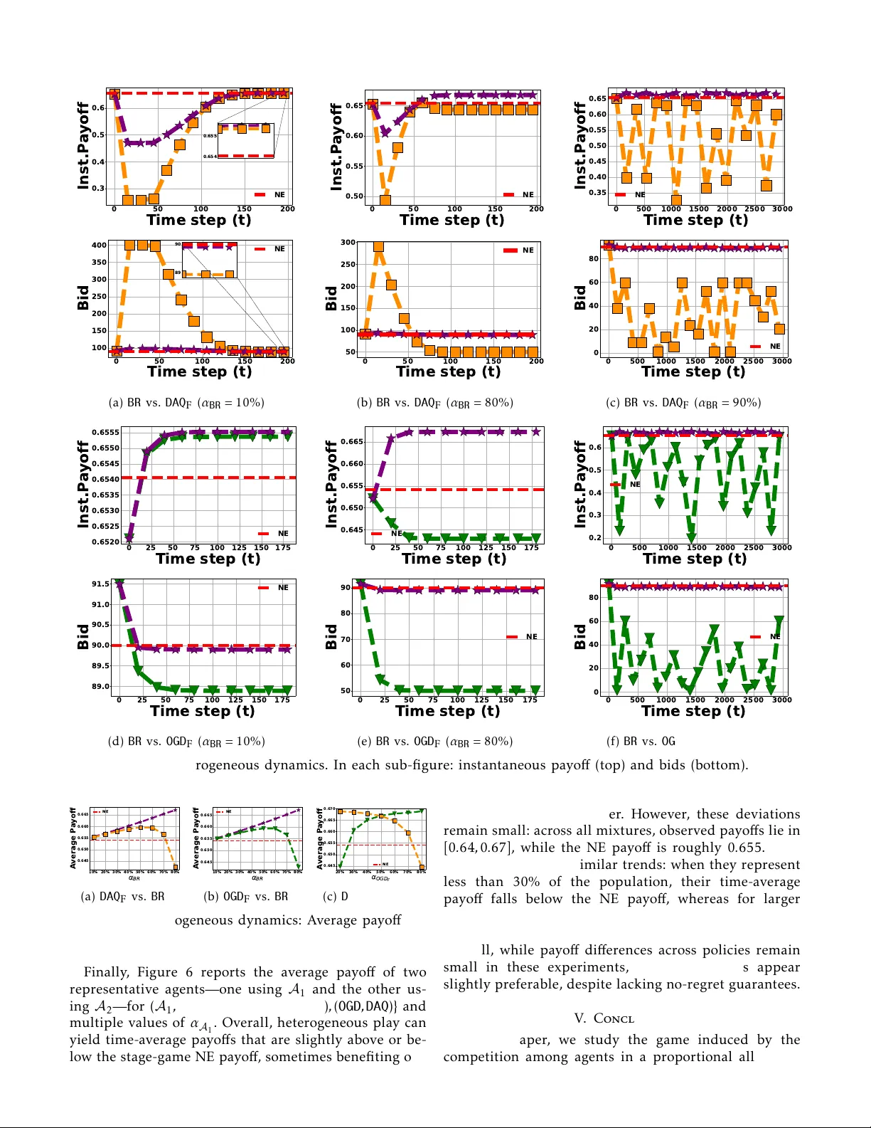
Loading high-quality paper...
Comments & Academic Discussion
Loading comments...
Leave a Comment