Global Stability Analysis of the Age-Structured Chemostat With Substrate Dynamics

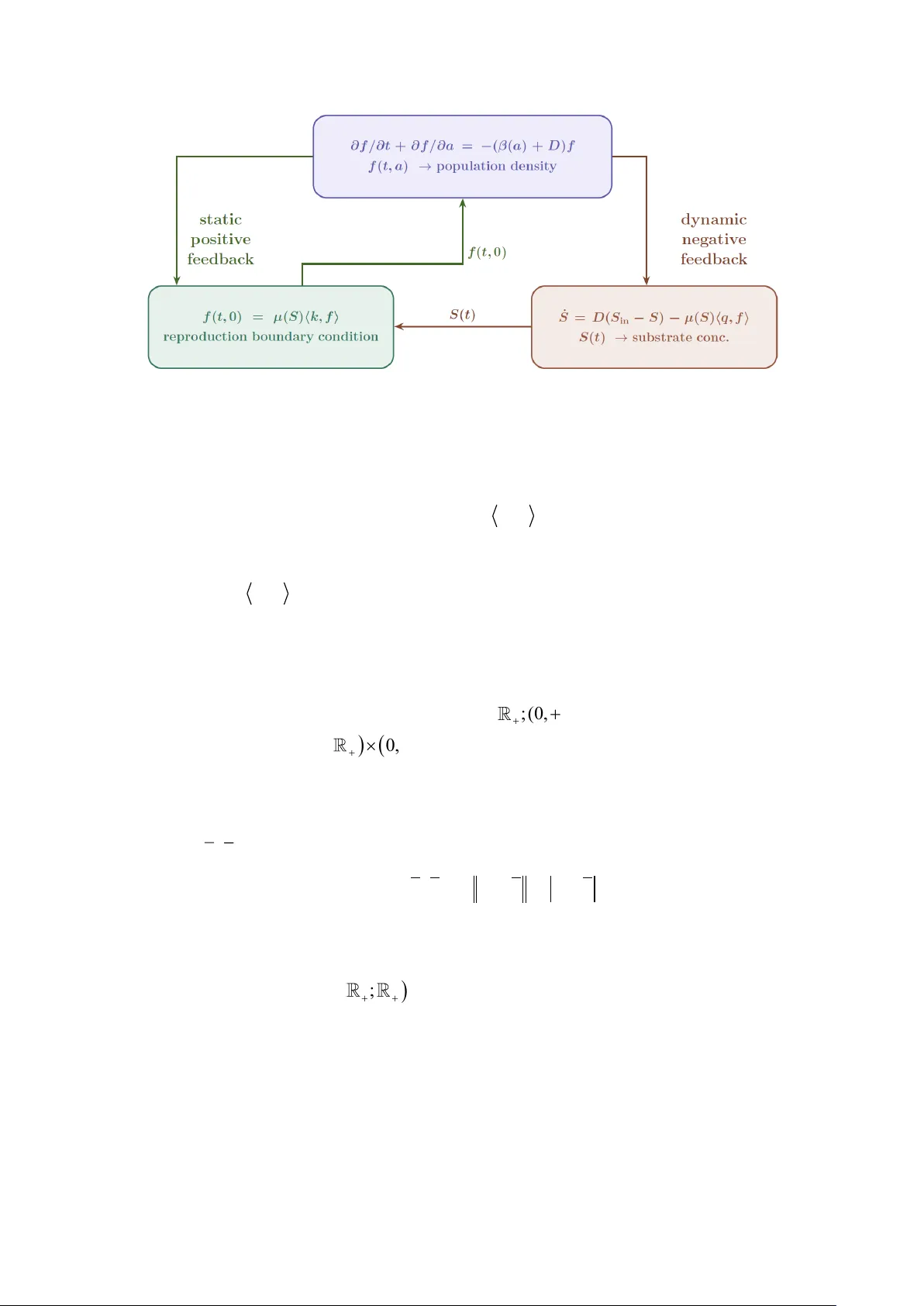
1 Global Stability Analysis of the Age-Structured Chemostat With Substrate Dynamics Iasson Karafyllis * , Dionysios Theodosis * , and Miroslav Krstic ** * Dept. of Mathematics, National Technical University of Athens, Zografou Campus, 15780, Athens, Greece, emails: iasonkar@central.ntua.gr , dtheodp@central.ntua.gr ** Dept. of Mechanical and Aerospace Eng., University of California, San Diego, La Jolla, CA 92093-0411, U.S.A., email: krstic@ucsd.edu Abstract In this paper we study the stability prope rties of the equilibrium point for an age-structured chemostat model with renewal boundary condition and coupled substrate dynamics under constant dilution rate. This is a complex infinite-dimensional feedback system. It has two feedback loops, both nonlinear. A positive static loop due to reproduction at the age-zero bound ary of the P DE, counteracted and dominated by a negative dynamic loop with the substrate dynamics. The derivation of explicit sufficient conditions that guarantee global stability estimates is carried out by using an appropriate Ly apunov functional. The constructed Lyapunov functional guara ntees global exponential decay estimates and uniform global asymptotic stability with respect to a measure related to the Lyapunov functional. From a biological perspective, stability arises because reproduction is constrained by substrate availability, while dilu tion, mortality, and substrate depletion suppress transient increases in biomass before age - structure effects can amplify them. The obtained r esults are applied to a chemostat model fro m the literature, where the derived stabili ty condition is compared with existing results that are based on (necessarily local) linearization methods. Keywords: Age-structured chemostat, PDEs, Lyapunov functional, Globa l Asymptotic Stability 2 1. Introduction Chemostat models c onstitute a fundamenta l fr amework for describing microbial growth in a bioreactor wit h continuous nutrient in flow and outflow. Classical chemostat models use a single varia ble to represent the microorganisms leading to systems of ordinary differential equations (see for instance [ 1] , [ 3], [25], [29]). However, in many biological syste ms the evolution of the population of microor ganisms depends strongly on their age. Incorporatin g age structure leads to infinite-dimensional models desc ribed by first-order hyperbolic partial differe ntial equations with renewal boundary conditions like the we ll-known Mc Kendrick-von Foerster equation (see [ 7] , [23] ). This additional structure substantially alters the qualitative behavior of the system. In contrast to cl assical ODE formulations with constant yield coefficients , age-structured models may exhibit oscillatory behavior that can reproduce experimentally observe d data (see [26], [32], [33]). When the age distributi on is coupled with substrate dynamics, the mathematical structure be comes considerably more invol ved. The resulting system c onsists of a transport Partial Differential E quation (PDE) for the popul ation ag e densit y and a nonlinear ordinary diffe rential equation for the substrate, c oupled with the PDE through nonlocal terms (see for instance [18], [32] , [33]). This nonlinear and nonlocal coupling introduces substantial analyt ical difficulties, especially in the study of global qualitative properties such as boundedness, attractivity, and asymptotic stability. For chemostat models described by finite-dimensional system s, equilibrium analysis and stability properties are well understood (see for instance, [1], [ 5] , [27 ], [29]). In contrast, for age-structured chemostats, existing results are sparse and deal only with local stability prope rties (obtained via lineariz ation techniques), or deal with settings in which the substrate equation is a bsent (se e for instance [11] , [12], [13] , [10], [24] , [25] , [32], [33]). Establishing global stability for the age-struc tured che mostat with substrate dynamics therefore remains substantially more challenging, due to the no nlinear and nonlocal interactions and the positivity constraints inhere nt to population dynamics. The obje ctive of thi s work is to p rovide su fficient conditions for unif orm global asymptotic stability of the equilibrium point for an age-structu red chemostat model. We provide global KL stability estimates for an age-structured chemostat model coupled with substrate dynamics under constant dilution rate. Though no fee dback law is being designed in the paper, the paper conducts nonlinear infinite-dimensional feedback analysis. The mode l has two nonlinear feed back loops. One is a positi ve static feedback loop due to re production at the birt h boundary condition of the PDE, while the other loop is dynamic and negative through the substrate dynamics. The main analytical challenge lies in quantifying, using tools that extend far b eyond the conventional small -gain theorem concepts, the interaction between these two loops and e stablishing conditions under which the negative feedback dominates. To address this challenge, our approach leverages the recent results obtained in [18] , that established global existence of solutions. Under suitable structural assumptions linking the birth and substrate consumption rates, we first show th e exi stence of a trapping (absorbing) region that is reache d by all solutions in finite time. We then 3 construct a Lyapunov fun ctional and derive e xplicit suff icient conditions that guarantee a global KL stability estimate with re spect to a spe cific measure. The construction of the Lyapunov functional combines deviations of the age p rofile with logar ithmic transformations of the normalize d substrate and reproduction rates, a llowing us to deal with the nonlinear and nonlocal terms of the model. The result establ ishes global exponential decay estimates and convergence of the age distribution together with the substrate concentration . The provided sufficient conditions for global asymptotic stability are explicit and can be readily verified from the model data, making them applicable in a wide ra nge of cases. In intuitive an d biological terms, we pr ove that the equilibrium is globally asymptotically stable, under suitable conditions, due to reproduction being constrained by substr ate ava ilability, and due to the combined effects of dilution, mortality, and substrate depl etion providing sufficient negative feedback to damp a ny temporary increase in biomass fa ster than age-cohort effects can build up self-sustaining oscillations. Finally, as an illust ration, we apply the derived stability theorem to a spe cific age-structured chemostat model studied in [32], for which local attractivity was established via linearization, and compare the local criteria given in [32] with the global stability condition obtained in our work. The paper is o rganized as follows. Section 2 introduces the model and presents its basic properties. Section 3 provides the main results, including the existence of a trapping region and the global KL stability esti mates. Section 4 provides an illu strative example and c omparison with existing results. Section 5 c ontains the proofs of the main results. Finally, some concluding remarks are given in Section 6. Notation Throughout this paper, we adopt the following notation.  : [0 , ) + = +  . For a vector n x   , x denotes it s Euclidean norm. We use the notation x + for the positive part of the real number x   , i.e., ( ) ma x , 0 xx + = .  Let n A   be an open set and let n B   be a set that satisfies () A B cl A  , where () cl A is the closure o f A . By 0 ( ; ) CB  , we d enote the class of continuous functions on B , which tak e values in m   . By ( ; ) k CB  , where 1 k  is an integer, we denote the class of functions on n B   , which take v alues in m   and have continuous derivatives of order k . In oth er words, the functions of class ( ; ) k CB  are the functions whic h have continuous derivatives of order k in int( ) AB = that c an be continue d c ontinuously to all points in AB  . W hen =  then we write 0 () CB or () k CB .  Let n A   be an open set and let m   be a non-empty set. By ( ) ; p LA  with 1 p  we denote the equivale nce class of measurable functions : fA → for which 1/ () p p p A f f x dx  =  +     . By ( ) ; LA   we denote the equivalence class of 4 measurable functions : fA → for which ( ) sup ( ) xA f f x   =  + where ( ) sup ( ) xA fx  is the essential supremum. When m =  we simply write ( ) p LA . When n B   is not ope n but has non-empty interior, ( ) ; p LB  a nd ( ) ; LB   mean ( ) ; p LA  and ( ) ; LA   , respectively, with int( ) AB = . By ( ) ; loc L  +   we denote the equivalence class of measurable functions : f + →  with   ( ) 0 , ; f L T   for every 0 T  .  By K we denote the class of increasing 0 C functions : a ++ →  with (0) 0 a = . By K  we denote the class of increasing 0 C functions : a ++ →  with (0) 0 a = and li m ( ) s as →+ = + . By KL we denote the set of all continuous functions :  + + + →  with the following pro perties: (i) for each 0 t  the mapping ( , ) t   is of class K ; (ii) for each 0 s  , the mapping ( , ) s   is non-in creasing with li m ( , ) 0 t st  →+ = .  Let I +   and let : fI ++  →  be a given function. We use the notation [] ft to denote the profile at certain tI  , i.e., ( [ ] )( ) ( , ) f t a f t a = for all 0 a  .  Let ( ) kL  +   and ( ) 1 fL +   be given. We define 0 , : ( ) ( ) k f k a f a da + =  . 2. The Age-Structu red Chemost at Mode l Consider the age-structured chemostat model ( ) ( , ) ( , ) ( ) ( ) ( , ) ff t a t a a D t f t a ta   + = − +  (2.1) ( ) ( , 0) ( ) , [ ] f t S t k f t  = (2.2) ( ) ( ) ( ) ( ) ( ) ( ) , [ ] in S t D t S S t S t q f t  = − −  (2.3) where ( , ) 0 f t a  is the distributi on function of the microbial population in the chemostat at time 0 t  and age 0 a  , ( ) 0 St  is the limiting substrate concentra tion, 0 in S  is the inlet concentration of the substrate, ( ) 0 Dt  is the dil ution rate, ( ) S  is the speci fic growth r ate function, () a  is the mortality rate and ( ), ( ) k a q a are functions that determine the birth of new cells and the substrate consumption of the microbial population, respectively. All functions , , , : kq  ++ →  are assumed to be bounded, ( ) 0 C +  functions with ( ) 1 C  +   , (0) 0  = , ( ) 0 S   for 0 S  and 0 ( ) 0 k a da +   , 0 ( ) 0 q a da +   . 5 Figure 1: Feedback structure of the age-structured chemostat model (2.1), (2.2), (2.3). The interconnection structure of system (2.1) , (2.2), (2.3) is il lustrated in Figure 1. From a control syst ems perspective, the model can be viewed as the interconnec tion of two feedback loops. The first loop is a positive feedback associated with the boundary condition (2.2), where the reproduction rate , kf drives the inflow of newborns $f(t,0)$ and, h ence, also the subsequent age distri bution ( , ) f t a . The second loop is a dynamic negative feedback through the sub strate equation (2.3), where the consumption , qf reduces t he substrate concentrati on () St , which in turn limits reproduction via the growth function () S  . This feedbac k interaction plays a central role in the stability analysis. Define: ( ) ( ) ( ) ( ) ( ) 0 1 0 ; ( 0 , ) , lim ( ) 0 , 0 , : (0) ( ) ( ) ( ) a in f C f a X f S L S f S k a f a da  + →+ + +   +  =  =    =      (2.4) We consider X to be a metric space with metric given by the formula for all ( ) ( , ), , f S f S X  : ( ) ( ) 1 ( , ), , d f S f S f f S S = − + − (2.5) We next provide the notion of solution that is appropriate f or system (2.1), (2.2), (2.3). Definition 1: Let ( ) ; loc DL  ++   , ( ) 00 , f S X  and 0 T  be given. We say that a continuous mapping ( )   , : 0, f S T X → is a weak solution on   0, T with input D of the initial-boundary value problem (2.1), (2.2), (2.3) with initial condition 00 [0] , (0) f f S S == (2.6) if the following properties are valid: i) (2.6) holds, 6 ii)   ( ) ( ) 0 0 , ; 0 , f C T +   +   and   ( ) : 0, 0, in S T S → is absolutely continuous, iii) (2.2) holds for all   0, tT  and (2.3) holds for [0, ] tT  a.e. iv) the follow ing equati on holds for all   ( )   ( ) 1 0 , 0 , C T L T   ++      with   ( ) 0, LT at   +   +       and   0, tT  : ( ) 0 0 0 0 00 ( ) (0, ) ( , 0) ( , 0) ( , ) ( , ) ( ) ( ) ( , ) ( , ) ( , ) ( , ) t t f a a da f s s ds f t a t a da a D s s a s a s a f s a da ds as      + + + +=   + + − −        (2.7) We say that the initial-boundary value problem (2.1), (2.2) , (2.3), (2.6) admits a global weak solution with input D if for every 0 T  there exists a weak solution on   0, T with input D of the initial-boundary value problem (2.1), (2.2), (2.3), (2.6). Next, we highlight a list of properties for the age-structured chemostat model (2.1), (2.2), (2.3) and its solutions. Properties : 1) Theorem 1 in [18] shows that for any ( ) 00 , f S X  , ( ) ; loc DL  ++   the weak solution ( ) [ ], ( ) f t S t with input D of the initial-boundary value problem (2.1), (2.2), (2.3), (2.6) is unique and is defined for all 0 t  . Notice that for const ant dilution rate ( ) 0 D t D  , : (0 , ) in SS + →  is continuously differentiable. 2) Definition (2.4) of the state space X (the facts that ( ) 0 ; ( 0 , ) fC +  +  and ( ) lim ( ) 0 a fa →+ = ), implies that ( ) XL  +    . Consequently, (since 1/ 1 1/ 1 pp p f f f −   for every   1, p  + and e very ( ) ( ) 1 f L L  ++    ) it follows that ( ) p XL +    for all   1, p  + . Thus, for any ( ) 00 , f S X  , ( ) ; loc DL  ++   the weak solution ( ) [ ], ( ) f t S t with input D of the initial-boundary value problem (2.1), (2.2), (2.3), (2.6) satisfies for all 0 t  and   1, p  + : ( ) [] f t L  +   (2.8) 1/ 1 1/ 1 [ ] [ ] [ ] pp p f t f t f t −   (2. 9) 3) Let ( ) 0 D t D  (a constant) be given and assume that the growth rate function () S  is increa sing. An equilibrium point for (2.1), (2.2), (2.3) that corresponds to the 7 (constant) dilution rate D consists of a point ( ) 0, in SS   that satisfies the so-called Lotka-Sharpe condition ( ) ,1 S k r   = (2.10) and has the equilibrium distribution function given for 0 a  by the formula ( ) ( ) ( ) ( ) , in D S S f a r a S q r     − = (2.11) where 0 ( ) exp ( ) a r a Da s ds   = − −     (2.12) 4 ) If we assume that ( ) ( ) 1 k C L  ++    with ( ) kL  +    then by taking ( , ) ( ) t a k a  = we obtain from (2.7) for ( ) 0 D t D  : ( ) ( ) 0 0 0 0 0 0 0 , (0) ( , 0) , [ ] ( ) ( ) ( ) ( , ) , [ ] , [ ] , [ ] , [ ] tt t t t k f k f s ds k f t a D k a k a f s a da ds k f t k f s ds D k f s ds k f s ds   +  + = + + −  = + + −       (2.13) Since the map ( ) ,: f S X + →  is continuous, it follows from (2.5) that the map ( ) 1 : f L ++ →  is continuous. It follows from (2.13) and the facts that ( , 0 ) t f t   is continuous and ( ) ,, k k L   +    , that the map , [ ] t k f t  is continuously differe ntiable and in conjunction with (2.2) satisfies the following equation for all 0 t  : ( ) ( ) ( ) , [ ] (0) ( ) , [ ] , [ ] , [ ] d k f t k S t D k f t k f t k f t dt   = − − + (2.14) Similarly, if we assume that ( ) ( ) 1 q C L  ++    with ( ) qL  +    then by taking ( , ) ( ) t a q a  = we obtain from (2.2), (2.7) for ( ) 0 D t D  that the map , [ ] t q f t  is continuously differentiable and sa tisfies the following equation for all 0 t  : ( ) ( ) , [ ] ( 0) ( ) , [ ] , [ ] , [ ] , [ ] d q f t q S t k f t D q f t q f t q f t dt   = − − + (2.15) 8 Finally, by taking ( , ) 1 ta   and recalling that ( , ) 0 f t a  for all ,0 ta  , we obtain from (2.2), (2.7) fo r ( ) 0 D t D  that the map 1 [] t f t  is continuously differentiable and satisfies the following equation for all 0 t  : ( ) ( ) 11 [ ] ( ) , [ ] [ ] , [ ] d f t S t k f t D f t f t dt  = − − (2.16) The following lemma provides some rough estimates for the weak solution ( ) [ ], ( ) f t S t with constant input D of the initial-boundary value problem (2.1), (2.2), (2.3), (2.6). Its proof is provided in Section 5. Lemma 1 : Let ( ) * , f S X   be an equilibrium point for (2.1), (2.2), (2.3 ) that corresponds to the constant input 0 D  . The n there exist constants ,0 RC  suc h that for every ( ) 00 , f S X  the weak sol ution ( ) [ ], ( ) f t S t with constant input D of the initial-boundary value proble m (2.1), (2.2 ), (2.3), (2.6) satisfies the follow ing estimates for all 0 t  : ( ) ( ) ( ) ( ) ( ) ( ) ( ) 00 [ ], ( ) , , exp , , , d f t S t f S R t d f S f S      (2.17) ( ) ( ) ( ) ( ) ( ) 0 0 0 [ ] m ax , exp , , , f t f f f C R t d f S f S      −  − (2.18) ( ) ( ) 0 ( ) exp in in S t S S S Dt  − − − (2.19) 3. Main Resu lts In this section we establish the main qualitative properties of the solutions of system (2.1) – (2.3) with constant dilution ( ) 0 D t D  . We first show the existence of an absorbing (trapping) region, that is reached by all solutions in finite time . We then investigate the stability prope rties of the e quilibrium introduced in Section 2 a nd prove convergence of solutions toward this equilibrium. We use the following assumptions: (A) There exists a constant 0 R  such that ( ) ( ) k a Rq a  for all 0 a  (3.1) (B) The function ( ) 1 C  +   is increasing, ,: kq ++ →  are bounded, ( ) 1 C +  functions with ( ) , k q L  +    , and there exist constants , b    , 0   , ,0   and continuous functions ,: hp ++ →  such that 9 ( ) ( ) ( ) ( ) ( ) ( ) ( ) ( ) ( ) ( ) ( ) ( ) q a a q a Dq a k a h a k a a k a q a bDk a p a        − − − =  − − − = (3.2) Assumption (A) requires that the ratio of the birth modulus k to the substrate consumption rate q is bounded from above. Such an assumption is just ified from a biological point of view, since only a p art of the substrate consumption is utilized for reproduction while the major part of substrate consumpti on is used for endurance. Assumption (B) imposes boundedness on the d erivatives of the birth and subst rate consumption rates which reflects the fact that reproduction and subst rate consumption vary smoothly with age a nd do not change abruptly as microorga nisms age. Moreover, assumption (B) introduces certain relations between () ka and () qa coupling their evolution with the mortality () a  and the dil ution D , where ( ), ( ) h a p a account for additional age-dependent factors that may affect the substrate consumption and the reproduction. Assumptions similar to assumption (B) have been used in the literature (see [15], [32] ). The following lemma shows the existence of a trapping region. Its proof is provided in Section 5. Lemma 2: Suppose that assumptions (A), (B) hold. Then for every in F R S  , where 0 R  is the constant involved in assumption (A), there exists an increasing continuous function : T ++ →  such that for every ( ) 00 , f S X  the weak solution ( ) [ ], ( ) f t S t of the initial-boundary value problem (2.1), (2.2), (2.3), (2.6) satisfi es for all ( ) 00 1 t T RS f + 1 ( ) [ ] RS t f t F + and () S t S  (3.3) where 2( ) in DS S D L F q   = + (3.4) and ( )     m a x : 0, in L S S S    = (3.5) Moreover, if 00 1 RS f F + and 0 SS  then (3.3) holds for all 0 t  . Let in F R S  be given and let 0 S  be defined by (3.4). We define the set:   1 : ( , ) : , f S X RS f F S S  =  +   (3.6) It is clear that Lemma 2 guarantees the set  defined by (3.6) is a trapping region of the age-structured chemostat model (2.1), (2.2), (2.3). Next, we introduce the scalar variables 10 ,, : , : , ,, q f k f q f k f   == (3.7) which represent the normalized substrate co nsumption and reproduction rates, respectively. It should be noticed that definition (2.4) and the fact that ,: kq ++ →  are continuous functions with 0 ( ) 0 k a da +   , 0 ( ) 0 q a da +   guarantees that ,0 qf  and ,0 kf  for all ( ) , f S X  . Therefore, definition (3.7) implies that ,0   for all ( ) , f S X  . To study the stability of the equilibrium ( ) , fS  , we introduce the followi ng normalized variables * () ( ) : , ( ) : ( ) ( ) (0) fa v a a v a r a f   = = − (3.8) where () ra is given by (2.12 ) and  given by (3.7). To capture the deviations of the substrate concentration from the equilibrium we also def ine : l n     =   , : ln in in SS w SS    − =  −  (3.9) Let also ( ) ( ) 12 (0) (0) ( ) , , ,, S qk gS q r k r S     = = = (3.10) Under a ssumption (B) equations (2.14), (2.15 ) a re valid. Combining (2.2), (2.3), (2.14), (2.15) (3.7), (3.8), (3.9), and (3.10), we obtain the equations ( ) ( ) ( ) ( ) (0) exp 1 1 g S g S  = − + − (3.11) ( ) ( ) ( ) ( ) ( ) ( ) ( ) ( ) ( ) 1 21 , exp 1 exp 1 , , 1 , pv gS qr ph gS qr           = + − − − + −      − + − − +  (3.12) ( ) ( ) ( ) ( ) ( ) ( ) ( ) ( ) ( ) ( ) 1 1 , exp 1 exp 1 1 , h w g S Dg S w D g S qr      = + − − − + − − +  (3.13) ( ) ( ) ( ) ( ) ( ) ( ) ( ) 1 exp 1 i n in S D S S g S D S S g S w = − − − − − −  (3.14) 11 For ( , ) f S X  , and , , , w      defined by (3.7), (3.8), and (3.9), resp ectively, w e introduce the following Lyapunov functional ( ) ( ) ( ) ( ) ( ) 22 0 , : exp 1 exp 1 ( ) ( ) 2 B V f S w w Q S a a da     + = − − +  − − + +  (3.15) where ( ) ( ) exp aa  =− (3.16) and ( ) : 0, in QS + →  is a continuously differentiable function that satisfies ( ) ( ) ( ) ( ) ( ) 1 : in gS Q S M S S g S −  = − (3.17) while , , 0, 0 BM     are constants which are to be selected. The functional : VX + →  defined by (3.15) is well defined for every ( , ) f S X  . The following theorem is the main result of the paper. Theorem 1 provides sufficient conditions for a global KL stability estimate with respect to the functional : X + →  defined by ( ) ( ) 1 , : , f S S S f f f f V f S      = − + − + − + (3.18) It should be noted that the functional ( ) , fS  defined by (3.18) has many features of a measure or more a ccurately, the analogue of the notion of a measure (or size function) used for finite-dimensional systems (see for instance [30], [31]) defined on open sets . More specifically, the functional ( ) , fS  defined by (3.18) satisfies ( ) ,0 fS  = and ( ) ,0 fS  for all ( ) ( )   , \ , f S X f S   and (as shown in Section 5 below ) ( ) , fS  → + as 0 S + → or in SS − → or 1 0 f + → or p ff  − → + for som e   1, p  + (r ecall (2.9 )). Th erefore, the functional ( ) , fS  “ blows up” when the state ( ) , f S X  approaches the “boundary” of the state space X . Theorem 1: Let in F RS  be given, let 0 S  be defined b y (3.4) and let  be the trapping region defined by (3.6). Assume that assumptions (A) and (B) hold with ( ) , :, , qr S q r kr   == (3.19) 12 Let 0   be a constant and define () a  by (3.16). L et ( ) 0 : inf ( ) a La   = and suppose that there exist constants, 1 2 3 , , 0 R R R  , 0   , 0   ,   0,1   , , , 0 BM  such that 2, qr     (3.20) ( ) ( ) 2 1 2 1 2, ph gS B q r      − − + (3.21) ( ) ( ) 11 2 2 2 2 2 21 1 , 2 2 , 2 h p h r L D r q r BR BR q r          −− −−   + +  + + +   (3.22) 12 B   (3.23) and the following matrix is positive definite: ( ) ( ) ( ) ( ) ( ) ( ) ( ) ( ) 1 1 2 1 2 2 11 3 2 1 2 1 1 / 2 / 2 / 2 / 2 2 , 2 / 2 / 2 1 in A Rh P D D DM g S q r R g S D DM DM Bg S           −  − −      = −  − −  + −       −  + −  − +   (3.24) where ( ) ( ) ( ) ( ) ( ) ( ) ( ) ( ) ( ) 2 11 1 1 3 2 1 1 2 1 1 2 2 , in in B A B B g S gS R R ph g S q r g S         − − = − + − + −  − − − Then, there exist a function CK   and a non-increasing function ( ) : 0 ,  + → +  such that for every ( ) 00 , f S X  the weak solution of the initial -boundary value problem (2.1), (2.2), (2.3), (2.6) satisfies the following estimate for all 0 t  : ( ) ( ) ( ) ( ) ( ) ( ) ( ) 0 0 0 0 [ ], ( ) exp , , f t S t C f S t C f S    −   (3.25) The proof of Theorem 1 is provided in Section 5. Remarks on Theorem 1 : (a) The functional ( ) Ψ, fS can be inte rpreted as a composite mea sure of the deviation from equilibrium. In particular, the deviation of f from * f is captured directly in the 13 1 L and L  norms, through a weighted 2 L - type term measuring the deviation o f a normalized age profile, and through quantities related to the birth and consumption rates. More precisely, ( ) Ψ, fS contains the direct terms * SS − ∣∣ , * 1 ff −  , and * ff  −  , together with the Ly apunov functional ( ) , V f S . The latter includes a weighted quadratic term measuring the deviation of the normalized age profile ( ) va from the normalized equil ibrium profile ( ) ra , as well as the logarithmic terms 1 e   −− and 1 w ew −− , where ( ) ln /    = measur es the deviation between normalized birth and normalized consumption ra tes, and w compares the substrate deficit ( in SS − ) with the norma lized consumption rate. Thus, Ψ mea sures not only the direct difference between ( , ) fS a nd ** ( , ) fS , but also the deviation of the normalized age prof ile from its equilibrium shape, together with the deviation between normalized birth a nd consumpti on ra tes, and between the substrate level and the normalized consumption. Estimate (3.25) of Theorem 1 guarantees glob al exponential convergence of the functional ( ) , fS  defined by (3 .18) and Uniform Global Asymptotic Stability with respect to the measure  . Definition (3.18) and inequality (2.9) show exponential convergence o f [] ft to f  in any p L norm with   1, p  + . Since ( ) ( ) ( ) ( ) , , , , d f S f S f S   (recall (2.5) and (3.18) ) estimate (3.25) shows global exponential convergence of the state to the equilibrium point in the metri c of the state space. The global KL stability estimate (3.25) and definition (3.18) of  can be exploited to conclude st andard (uniform) global asymptotic stability properties with respect to various metrics. (b) The suffi cient condi tions (3.20)-(3.24) that guarantee the global KL stability estimate (3.25) are expressed in terms o f the mod el data and auxiliary constants . The example in the following section illustrates their use and shows that the sufficient conditions (3.20)-(3.24) are not conservative. We next provide a more detailed interpre tation of these conditions: First, condition (3.20 ) requires the quantity 2, qr  to dominate the auxiliar y product  where , qr is a weighted integral of the subst rate consumption with respect to the normalized equilibrium prof ile () ra in (2.12). Since  a nd  a re auxiliary constants, their product can be chosen arbitrarily small and therefore, conditi on (3.20) can be satisfied without imposing any restrictive condition on the model parameters. Next, conditions (3.21) and (3.23) constrain the admissible values of th e weight B appearing in the integral term of the Lyapunov functional measuring the deviation of the age distribution from the equilibrium. Condition (3.21) may impose a lower requirement on B , ensuring that deviations of th e a ge distribution are penalized strongly enough in the Lyapunov e stimate. The lower bound in (3.21) reflects the need for the age- distribution term to c ompensate for the a dditional coupling effects generated by the functions , hp . Thus, B must be chosen sufficiently large so that deviations in 14 the age profile are pena lized strongly enough. On the other hand, condition (3.23) imposes an upper bound on B preventing this weight from becoming too large. Thus, conditions (3.21) and (3.23) require the existen ce of an admissible range o f values for B ensuring a proper b alance in the contribution of the age -distribution term to the Lyapunov functional. More specifically, the para meter   0,1   distributes certain coupling terms between these inequalities and the dissipation condition (3.22). When 0  = , condition (3.21) becomes nonrestrictive, while the terms multiplied by 1  − in (3.22) attain their maximal contribution. In this case, the functions ( ) ha and ( ) pa , which describe additional terms in the differential relations for ( ) qa and ( ) ka in (3.2), contribut e significantly to condition (3.22). Note that conditions (3.21) and (3.22) can be trivially satisfied when ( ) 0 ha  and ( ) 0 pa  . C onsequently, the parameters  and  , together with the minimal mortality ( ) 0 inf a La   = , must dominate the additional coupling effec ts generated by h and p in (3.22). For 0   , part of this influence is shifted to condition (3.21), thereby relaxing the diss ipation requirement in (3.22). Overall, conditions (3.20) – (3.23) ensure that the parameters of the Lyapunov func tional can be chosen so that the dissipative mechanisms d ominate the coupling e ffects arising from reproduction and substrate consumption. Finally, condition (3.24 ) require s a certain matrix P to be positive definite. This matrix appears in the estimate o f the Lyapunov derivative through a term involving a vector built from the deviations of the substrate c oncentration ( ) St a nd the auxiliary v ariables ( ) t  and ( ) wt . The positive de finiteness of P ensures that these deviations, taken together, are effectively controlled, so that no combination of S ,  , and w can offset their contribution in the stability estimate. 4. Illustrative Ex ample In this section we apply Theorem 1 to the age-str uctured chemostat model studied in [32] and derive an expli cit condition guaranteeing global asymptotic stability of the equilibrium. The model studied in [32] is given by ( ) ( , ) ( , ) ( , ) ff t a t a L D f t a ta  + = − +  (4.1) ( ) ( ) 0 ( , 0) exp ( , ) f t S Y k a f t a da  + =−   (4.2) ( ) ( ) 0 ( ) ( ) ( ) ( , ) in S t D S S t S t f t a da  + = − −   (4.3) 15 where 0 Y  , 0 k   , 0 L  , 0 D  and ( ) 1 C  +   , increasing with (0) 0  = , and ( ) 0 S   for 0 S  . Model (4.1), (4.2), (4.3) corresponds to system (2.1), (2.2), (2.3) with ( ) , ( ) 1 , ( ) ex p( ) a L q a k a Y k a    = −  (4.4) In this case ( ) exp( ( ) ) r a D L a = − + (4.5) while a straightforward calculation yields 1 ,, Y k r q r DL D L k == + ++  (4.6) The equilibrium is determined by the Lotka-Sha rpe condition (2.10), which, due to (4.6), in this case is given by the point (0, ) in SS   that satisfies ( ) D L k S Y   ++ =  (4.7) Using (4.6) and (2.11), the corresponding equilibrium for the a ge distribution is given by ( ) ( ) ( ) ( ) ( ) exp ( ) in Y D D L S S f a D L a D L k   +− = − + ++  (4.8) Proposition 1: Consider the age-structured chemostat model (4.1), (4.2), (4.3) with 0 Y  , 0 k   , 0 L  , 0 D  . Let * ( , ) fS  be the equilibrium defined by (4.7) and (4.8). If ( ) 2 82 k D Lk  +   (4.9) then, * ( , ) fS  is uniformly globally asymptotically stable with respec t to the measure  defined by (3.18). Remark on Proposition 1: It was shown in [32], that after the conversion of system (4.1), (4.2), (4.3) to a syst em of ordinary differential equations, its linearization gives local attractivity of the equilibrium under the condition that ( ) 2 8 k L D k −    (4.10) On the other hand, condit ion (4.9) and e stimate (3.25) establish (uniform) global asymptotic stability of the equilibrium (4.7), (4.8). Notice that when 3 2 k L   , condition (4.9) is more conservative than (4.10), whereas, when 3 2 k L   , condition (4.9) is less conservative than (4.10). Both conditions give the same limi t condition /8 Dk   as 0 L + → (when the morta lity rate is negligible), which means that there must be roug hly eight generations of organisms in the chemostat for instability of the equilibrium to be possible. 16 5. Proofs In this se ction we provid e the proofs of all results . We start with the proof of Lemma 1. Proof of Lemm a 1: Let arbitrary ( ) 00 , f S X  and 0 D  be given and consider th e weak solution ( ) [ ], ( ) f t S t with input D of the initial-boundary value problem (2.1), (2.2), (2.3), (2.6). Let also ( ) * , f S X   be an equilibrium point for (2.1), (2.2), (2.3) that corresponds to the const ant input 0 D  . Using the boundary condition (2.2) and that at equilibrium we have ( ) (0) ( ) f a f r a  = , we get by Lemma 1 in [18] a nd (2.11), (2.12) that ( ) ( ) 0 0 ( ) ( ) exp ( ) 0 ( , ) ( ) ( ) (0) exp ( ) 0 a at a f a t f a t Dt s ds for t a f t a f a x t a f Da s ds for t a    −     − − − − −        −=    − − − −          (5.1) where ( ) ( ) ( ) , [ ] x t S t k f t  = . Using (5.1) we get ( ) ( ) ( ) 1 0 00 0 00 0 [ ] ( , ) ( ) ( , ) ( ) ( ) ( 0) exp ( ) exp ( ) ( ) exp ( ) exp ( ) (0) exp ( ) exp ( ) ( ) exp t t ta a t a t t t l f t f f t a f a da f t a f a da x t a f Da s ds da Dt f a t f a t s ds da Dt x l f Dl s ds dl Dt f l f l    +     +  − −   − = − + −  = − − − −    + − − − − −    = − − −   + − −     0 () tl l s ds dl  + +  −    (5.2) Since ( ) 0 a   , 0 a  , 0 D  we obtain from (5.2) the following estimate 0 11 0 [ ] ( ) ( 0) t f t f x l f dl f f    −  − + −  (5.3) 17 Recall that ( ) ( ( )) , [ ] x t S t k f t  = and (0) ( ) , f S k f     = . Then, since  is bounded and since kL   we get ( ) ( ) ( ) ( ) ( ) max 1 ( ) (0) ( ) , [ ] , ( ) , [ ] , ( ) [ ] , ( ) x t f S t k f t S k f S t k f t f k f S t S k f t f k f L S t S                 − = −  − + −  − + − (5.4) where ( )     m a x : 0 , in L S S S    = and ma x () in S  = (recall that  is increasing and ( ) (0, ) in S t S  for all 0 t  ). Using (5.3) and (5.4) we obtain the following estimate ma x 0 1 1 1 00 [ ] [ ] , ( ) tt f t f k f l f dl f f k f L S l S dl         −  − + − + −  (5.5) Since ( , ) fS  is an e quilibrium o f (2.1), (2.2), (2.3), equation (2.3) can also be written as ( ) ( ) ( ) ( ) ( ) ( ) , [ ] , S t D S t S S t q f t S q f     = − − − +  which gives ( ) ( ) ( ) ( ) ( ) ( ) 0 0 ( ) exp exp ( ) ( ) , [ ] , t S t S Dt S S D t l S l q f l S q f dl    − = − − − − − −  (5.6) Using the fact that qL   and definitions ( )     m a x : 0 , in L S S S    = and ma x () in S  = we directly obtain from (5.6) that ( ) ( ) ( ) ( ) ( ) 0 0 0 00 0 ma x 1 00 ( ) ( ) , [ ] , ( ) , [ ] , ( ) [ ] , ( ) t tt tt S t S S S S l q f l S q f dl S S S l q f l f dl q f S l S dl S S q f l f dl q f L S l S dl                    −  − + −  − + − + −  − + − + −    (5.7) Define ( ) ( ) ma x : max , , R k q q k f L     = + + . Estimate s (5.5) and (5.7) give for 0 t  that 18 ( ) 00 1 1 1 0 [ ] ( ) [ ] ( ) t f t f S t S f f S S R f l f S l S dl       − + −  − + − + − + −  (5.8) Inequality (5.8) and a direct applica tion of Gronwall-Bellman inequa lity imply that the following estimate holds for 0 t  ( ) ( ) 00 11 [ ] ( ) exp f t f S t S R t f f S S     − + −  − + − (5.9) Inequality (2.17) follows immediately from definition (2.5) and (5.9). Next, from formula (5.1), (5.4), (5.9) and the fact that ( ) 0 a   , 0 a  , and 0 D  we get   ( ) ( )   ( ) ( ) ( ) ( ) ( ) 0 0, 0 ma x 1 0, 0 ma x 0 0 1 [ ] max , ma x ( ) (0) ma x , ma x , , max [ ] ( ) ma x , max , , exp lt lt f t f f f x l f f f k k f L f l f S l S f f k k f L R t f f S S                        −  − −     − − + −    − − + − (5.10) Inequality (2.18) is a cons equence of (5.10) and definition ( 2.5) with ( ) ma x m ax , , C k k f L     = . Since ( ) 0 S   for 0 S  , and ,0 kf  for all ( ) , f S X  , equation (2.2) gives ( ) ( ) ( ) in S t D S S t  −  , 0 t  , from which (2.19) follows directly. The proof is complete.  W e next provide the proof of Lemma 2. Proof of Lemm a 2: Let ( ) 00 , f S X  . By virtue of Theore m 1 in [18], the weak solution ( ) [ ], ( ) f t S t X  of the initial-boundary value problem (2.1), (2.2), (2.3), (2.6) is unique and is defined for all 0 t  . Define 1 ( ) : ( ) [ ] Y t RS t f t =+ , for 0 t  (5.11) Using (2.3), (3.1), (2.16), definition (5.11) and the fact that ( , ) 0 f t a  and ( ) 0 a   we get for all 0 t  ( ) ( ) ( ) ( ) ( ) ( ) 1 ( ) ( ) ( ) , , , ( ) ( ) , () in in in Y t D RS RS t S t Rq f f D f S k f D RS Y t S t k Rq f D RS Y t     = − − − − +  − + − −  (5.12) The differential inequality (5.12) gives the following estimate for all 0 t  : 19 ( ) ( ) ( ) (0) exp in in Y t RS Y RS Dt  + − − (5.13) Define: ( ) ( ) 00 1 1 0 0 1 , : ln 1 in RS f F T f S D F RS +  +−  =+  −  (5.14) Then (5.13) and (5.14) guarantee that 1 ( ) ( ) [ ] Y t RS t f t F = +  for all ( ) 1 0 0 , t T f S  . Moreover, if 00 1 (0) Y RS f F = +  then 1 ( ) ( ) [ ] Y t RS t f t F = +  for all 0 t  . Since 1 [ ] ( ) f t Y t  (recall (5.11)), it follows that 1 [] f t F  for all ( ) 1 0 0 , t T f S  (5.15) Using the facts that ( ) (0, ) in S t S  for all 0 t  , (5.15), ( ) () sup : 0, in S S S L S       (a consequence of (3.5) and the fact that ( ) 00  = ), (3.4) and boundedness of q , we get for every ( ) 1 0 0 , t T f S  : ( ) ( ) ( ) ( ) ( ) ( ) ( ) 1 ( ) ( ) ( ) , ( ) ( ) [ ] ( ) ( ) () 2 ( ) in in in in S t D S S t S t q f DS DS t q S t f t DS DS t F q S t DS D L F q S t D L F q S S t          = − −  − −  − −  − + = + −  (5.16) Then, from (5.16) we obtain the following estimate for ( ) 1 0 0 , t T f S  : ( ) ( ) ( ) ( ) ( ) ( ) ( ) 1 0 0 1 0 0 ( ) 2 , 2 exp , S t S S T f S S D L F q t T f S    + − − + − (5.17) Estimate (5.17 ) guarantees that if 00 1 RS f F + (w hich implies ( ) 1 0 0 ,0 T f S = ; re call (5.14) ) and 0 (0) S S S = then 1 ( ) ( ) [ ] Y t RS t f t F = +  and () S t S  for all 0 t  . Estimate (5.17) guarantees that () S t S  for all ( ) 20 t T f  , where ( ) ( ) ( ) 2 0 0 1 0 0 ln 2 , : , T f S T f S D L F q   =+ + (5.18) Combining (5.18) and (5.14), we con clude that (3.3) h olds with ( ) ( ) ( ) ln 2 1 : ln 1 in sF Ts D F RS D L F q  +   − = + +   −+  for 0 s  . The proof is complete.  20 The proof of Theorem 1 requires certain auxili ary results. The following lemma provides additional estimates for the solutions of (2.1), (2.2), (2.3). Lemma 3: Suppose that assumpti ons (A), (B) hold. Then 1 b  , 1   and for every ( ) 00 , f S X  the weak solut ion ( ) [ ], ( ) f t S t of the i nitial-boundary value problem (2.1), (2.2), (2.3), (2.6) satisfies the following estimates for all 0 t  ( ) ( ) ( ) exp 1 ( 0) t D b t  − (5.19) ( ) ( ) ( ) exp 1 ( 0) t D t    − (5.20) and ( ) ( ) 0 00 1 ( ) min , in in in DS S t S D L q RS RS f RS  +       + + + −  (5.21) Proof of Lemma 3: Equations (2.14), (2.15), (3.2) and definitions (3.7) give for every weak solution ( ) [ ], ( ) f t S t of (2.1), (2.2), (2.3): ( ) ( ) ( ) ( ) ( ) , , ( 0) ,, , , ( 0) 1 ,, qf pf k S bD D k f k f kf hf q S D q f q f                 = + − + + = + + − +   (5.22) At equilibrium, we obtain from (5.22) that ( ) ( ) ( ) ( ) ( ) ,, 1 ( 0) ,, ,, 1 ( 0) ,, q f p f D b k S k f k f h f k f D q S q f q f             − = − − − − = − − + The above equa tions together with the facts th at , , , , : k q h p  ++ →  are non- negative functions and 0   , ,0   guarantee that 1 b  and 1   . Moreover, equations (5.22) guarantee the following differential inequalities: ( ) ( ) 1 1 Db D     − −   (5.23) Estimates (5.19) and (5.20) are consequences of the differential inequa lities (5.23). 21 Equation (5.13) shows that the following estimate holds for all 0 t  : ( ) 00 1 1 [] in in f t RS RS f RS +  + + − (5.24) Using (2.3), (3.5), and (5.24) we get for all 0 t  : ( ) ( ) ( ) ( ) ( ) 1 1 00 1 ( ) ( ) ( ) , ( ) ( ) [ ] ( ) [ ] ( ) () in in in in in in S t D S S t S t q f DS DS t q S t f t DS DS t L q f t S t DS D L q RS RS f RS S t       +  = − −  − −  − −   − + + + −    (5.25) Differential inequality (5.25) implies the following estimate for all 0 t  : ( ) ( ) ( ) ( ) ( ) ( ) 0 0 0 1 00 1 00 1 ( ) exp 1 exp in in in in in in in S t S D L q RS RS f RS t DS D L q RS RS f RS t D L q RS RS f RS    +  +  +     − + + + −        − − + + + −       + + + + − Estimate (5.21) is obtained from the above estimate. The proof is comple te.  Next, we give some useful lemmas for the functional V define d by (3.15). Lemma 4 below shows first that V define d by (3.15) is differentiable along the weak solutions of (2.1), (2.2), (2.3), (2. 6) with constant input D and provides the ex act derivative formula of the Lyapunov functional. Lemma 4: Suppose that assumption (B) holds. Let arbitrary ( ) 00 , f S X  be given and consider the w eak solution ( ) [ ], ( ) f t S t with input D of the initial-boundary value problem (2.1), (2.2) , (2.3), (2.6). Then the map ( [ ] , ( )) t V f t S t  , 0 t  is differentiable and the derivative of the L yapunov functional ( , ) V f S along the w eak solution ( ) [ ], ( ) f t S t , 0 t  , satisfies the following equation for 0 t  : ( ) ( ) ( ) ( ) ( ) ( ) 2 0 2 2 2 ( [ ], ( )) exp ( ) 1 ( ) e xp ( ) 1 ( ) () ( ) ( , ) ( ) ( , ) ( ) ( ) () ( ( )) ( ) ( , 0) 2 d V f t S t t t w t w t dt t B a t a a D t a r a r a da t B Q S t S t t B           + = − +  −     − + + + +       + + −      (5.26) 22 Proof of Lem ma 4: Let arbitra ry ( ) 00 , f S X  be given and consider the weak solut ion ( ) [ ], ( ) f t S t with constant input D of the initial-boundary value problem (2.1), (2.2), (2.3), (2.6). Define ( ) ( ) ( ) , [ ] x t S t k f t  = , 0 t  . Using the boundary condition (2.2) and that at equilibrium we have ( ) (0) ( ) f a f r a  = , we get by Lemma 1 in [18] and (2.11), (2.12) that ( ) ( ) 0 () ( ) ( ) 0 () ( , ) ( ) ( ) (0) ( ) 0 ra f a t f a t for t a r a t f t a f a x t a f r a for t a     − − −    − −=   − −    (5.27) Next, recalling fr om (3.8) that * () ( ) ( ) (0) fa a r a f   =− the Lya punov functional in (3.15) can be written as ( ) ( ) ( ) ( ) ( ) ( ) ( ) ( ) ( ) ( ) 2 2* 2 2* 0 2 2 2 2 * 2 2 * 00 , exp 1 e xp 1 ( ) ( ) ( ) 2 (0) 11 ( ) ( ) ( ) ( ) ( ) ( ) 2 (0) V f S w w Q S B a f a f a da f BB a r a da a r a f a f a da f       + + + = − − +  − − + +− −− + − −   (5.28) Splitting the first and last integra l of (5.28) at at = , we get, via (5.27) and a change of variables ta  =− , that ( ) ( ) ( ) 2 * 2 2 00 2 2 0 0 ( ) ( ) ( , ) ( ) ( ) ( ) ( ) ( 0) () ( ) ( ) ( ) () t a r a f t a f a da t s r t s x s f ds rt t f f d r         +  +  − = − − − + + + −   (5.29) ( ) ( ) ( ) 22 2 * 2 2 00 2 2 2 0 2 0 ( ) ( ) ( ) ( ) ( ) ( ) (0) () ( ) ( ) ( ) () t a f a f a da t s r t s x s f ds rt t f f d r         +  +  − = − − − + + + −   (5.30) Combining (5.28), (5.29), and (5.30) we get 23 ( ) ( ) ( ) ( ) ( ) ( ) ( ) ( ) ( ) ( ) 2 22 2 2* 0 2 2 2 0 22 2* 0 2 2 2 2 2 2 * 0 ( [ ], ( )) exp ( ) ( ) 1 exp ( ) ( ) 1 ( ) ( ) ( ) ( ) (0) 2 ( ) (0) () ( ) ( ) ( ) () 2 ( ) (0) ( ) 1 ( ) 1 ( ) ( ) ( ) 2 ( ) ( ) (0) t V f t S t t t w t w t Q S t B t s r t s x s f ds tf B r t t f f d r tf B t B t a r a da t s t t f                +  + = − − +  − − + + − − − + + + − −− + − −    ( ) ( ) ( ) 2 0 2 2 0 2* 0 ( ) ( ) ( 0) ( ) 1 () ( ) ( ) ( ) () ( ) (0) t r t s x s f ds Bt rt t f f d r tf           +  −− − + − + −   Using Leibniz’s integral rule and equations (2.11), (2.12), (3.8) , (3.11), (3.16), (5.29) and (5.30) we obtain (5.26). The proof is complete.  Next, we give a technical lemma whose proof c an be found in the appendix. We use the notation 2 (0) W  for the Hessian matrix at 0 n O   of a function of 2 () W C O  , where O is an open set. Lemma 5: Let n O   be an o pen set with 0 O  . Suppose that ( ) 2 W C O  is a positive definite function with 2 (0) W  being positive definite and such that the set   : ( ) x O W x r  is compact for all 0 r  . Then there exists a non-decreasing function : p ++ →  such that ( ) 2 ( ) ( ) W x p W x x  for all xO  . The following lemma exploi ts Lemma 5 and establishes some useful estimates for the Lyapunov functional V in (3.15). Lemma 6: There exist non-decreasing functions :  ++ →  , : (0 , )  + → +  such that the following inequalities holds for all ( ) , f S X  : ( ) ( ) ( ) ( ) ( ) 1 / 2 , (0) , , S k f f S S V f S V f S   − + −  (5.31) ( ) ( ) ( ) , , ( , ) V f S V f S E f S   (5.32) where ( ) ( ) ( ) ( ) ( ) 22 2 2 2 ( , ) exp 1 exp 1 ( ) 1 E f S w g S   = − + − + − + (5.33) Proof of Lemma 6: Let , w  as defined by (3.9). Notice that from (2.2 ) we get the equilibrium relation (0) ( ) , f S k f     = . Using definitions (3.9) , (3.10), and the previous equality, we get 24 ( ) ( ) ( ) ( ) ( ) , (0) ( 0) exp 1 in in S S g S S k f f f w SS     −  − = + −  −  (5.34) By adding and subtracting terms, (5.34) gives ( ) ( ) ( ) ( ) ( ) ( ) ( ) ( ) ( ) ( ) ( ) ( ) ( ) ( ) ( ) ( ) ( ) ( ) ( ) ( ) ( ) ( ) ( ) ( ) ( ) ( ) , (0) ( 0) exp 1 (0) exp 1 exp 1 (0) exp 1 (0) (0) in in in in in in in in in S S g S S k f f f SS S S g S fw SS S S g S fw SS f S S f S S S S S S S S S                 − − = − − − + − − − − +− − − + − + − −− (5.35) For (0, ) in SS  , by using the fa ct th at () gS is increasing (since  is increasing) and definition (3.5), we get ( ) ( ) ( ) ( ) ( ) ( ) ( ) ( ) ( ) ( ) ( ) ( ) ( ) , ( 0) ( 0) exp 1 (0) exp 1 exp 1 (0) (0) exp 1 1 in in in in in in in in in in in S g S S k f f f SS S g S fw SS SL S g S f f w S S S S S S S              −  − − + − − −   + − + + −  −−  (5.36) Due to Lemma 5, there e xists a non-decreasing function : p ++ →   such that ( ) ( ) 2 exp( ) 1 e x p ( ) 1 y y y p y y  − − − −  for all y   . Using the inequality ( ) ex p( ) 1 e xp y y y − that holds for all y   , we get ( ) ( ) 1 / 2 exp ( ) 1 exp( ) 1 exp ( ) 1 y y y y y  −  − − − − (5.37) for all y   with ( ) ( ) ( ) ( ) ( ) 1 / 2 1 / 2 1 / 2 ( ) : e xp s p s s p s  =  . Notice that :  ++ →  is a non-decreasing function. Using now (3.15) and (5.37) with y  = and yw = we get, respectively, ( ) ( ) ( ) ( ) ( ) 1 / 2 exp 1 , , V f S V f S  − (5.38) 25 ( ) ( ) ( ) ( ) ( ) 1 / 2 1 / 2 1 ex p 1 , , w V f S V f S  −− −    (5.39) Define for ( ) , in x S S S   − − : ( ) ( ) : x Q S x  = +  (5.40) where () QS satisfies (3.17). Then, using (3.17) and (5.40) we get that ( 0) 0 =  and ( ) ( ) ( ) ( ) ( ) 1 Sx in S gl x M dl S l g l   + − = −   (5.41) Notice now that ( ) ( ) ( ) ( ) ( ) ( ) ( ) ( ) ( ) ( ) ( ) ( ) ( ) 2 2 1 1 in in in g S x xM S S x g S x g S x S S x g S x g S x xM S S x g S x        +−  = − − +  + − − + + − +  = − − +   from which, the following properties are obtained ( ) ( ) ( ) ( ) 0 0 0 0 in x x x gS M SS         =  −   (5.42) where we have used the fact that () gS is increasing with ( ) 1 gS  = . Next, we show that the set ( )   , : ( ) in x S S S x r   − −   (5.43) is compact for all 0 r  . Since g is increasing, we can define   m a x ( ) : 0, L g S S S    =    , which gives for 0, SS     that () g S L S   . For 2 S Sx   −   − and by using the fact that g is increasing, inequalities () g S L S   , 1 ( ) 0 gS − , 0, SS     and (5.41), we get 26 ( ) ( ) ( ) ( ) ( ) ( ) ( ) ( ) ( ) ( ) ( ) ( ) ( ) / 2 / 2 11 1 / 2 1 1 1 / 2 ln 2 SS in in S x S x SS in in S x S x in g l g l MM x dl dl L S l l L S l M g S gl M dl dl L S l L S l M g S S L S Sx     ++  ++    −−   − − −   −    +        (5.44) For 2 in in SS S S x   − −   and by using similar arguments as above we also get that ( ) ( ) ( ) ( ) ( ) ( ) ( ) ( ) ( ) ( ) ( ) ( ) ( ) ( ) ( ) ( ) ( ) ( ) ( ) ( ) ( ) ( ) /2 /2 11 / 2 1 / 2 1 ln 2 in in S x S x in in in in S SS Sx in in in SS in in in in g l g l MM x dl dl g S S l g S S l M g S S dl g S S l M g S S SS gS S S x      ++ +  + +    −−   −− +−  −  +− −    −−     (5.45) Inequalities (5.44) and (5.45) show th at ( ) ( ) ( ) lim xS x +  →− = +   and ( ) ( ) ( ) lim in x S S x −  →− = +   , which imply that the set in (5.43) is compact for all 0 r  . Since the set in (5.43) is compact for all 0 r  and due to (5.42), it follows by Lemma 5, that there exists a non-decreasing function : p ++ →  such that ( ) ( ) 2 () x x p x   for all ( ) , in x S S S   − − . Thus, for x S S  =− , definition (5.40) gives ( ) ( ) 2 () S S Q S p Q S  − for all ( ) 0, in SS  (5.46) Now define ( ) ( ) 1 / 2 ( ) : s p s  =  , 0 s  . Since p is nondec reasing, so is   . Thus, since by (3.15) we have that ( ) ( , ) Q S V f S  , ( , ) f S X  , it follows that ( ) ( ) ( ) ( ) 1 / 2 , , S S V f S V f S   −  for all ( ) 0, in SS  (5.47) Combining (5.36), (5.38), (5.39), and (5.47), we finally obtain (5.31) with 27 ( ) ( ) ( ) ( ) ( ) ( ) ( ) ( ) ( ) ( ) 1 / 2 1 1 / 2 1 1 / 2 ( ) : ( 0) 1 (0) 1 in in in in in in in S g S r r f r r r SS SL S g S f r r S S S        −   −   = +  +   −       +  + +    −     Next, we show that (5.32) holds for some non-decreasing function  . Define ( ) ( ) ( ) 2 () 0, , ( ( ) 1 ) () 2 ( ) in in QS S S S S gS S M SS S S g S       −  =   =  −   (5.48) which due to (3.17) is continuous since 1 , g Q C  with ( ) 1 gS  = and ( ) 0 QS  = . Define also for 0 s    ( ) : sup ( ) : (0, ), ( ) Q in s S S S Q S s  =    which is non- decreasing and well define d for e ach 0 s  , by virtue of (5.40 ) and (5.43). Since ( ) ( , ) Q S V f S  for all ( , ) f S X  , it follows that ( ) 2 ( ) ( ( , )) ( ) 1 Q Q S V f S g S  − (5.49) Define for 0 s  ( ) 1 2 exp( ) 1 ( ) : sup : 0 , 1 exp( ) 1 y yy s y e y s y   −− =  − −    −  (5.50) which is we ll defined (due to the fact that the se t   : e xp( ) 1 y y y s  − −   is c ompact for all 0 s  ) and non-de creasing. F or any y   with exp( ) 1 y y s − −  , 0 s  , definition (5.50) implies that ( ) 2 1 ex p( ) 1 ( ) exp ( ) 1 y y s y  − −  − . Thus, ( ) ( ) 2 1 exp 1 ( ( , )) exp( ) 1 V f S     − −  − (5.51) ( ) ( ) 2 1 exp 1 ( ( , ) / ) exp( ) 1 w w V f S w  − −   − (5.52) Then due to (5.51), (5.52), (5.49) and (3.15) we obtain (5.32) with ( ) 11 ( ) : m a x ( ), ( / ), ( ), / 2 Q s s s s B     =   The proof is complete.  28 The following lemma establishes that the exponential de cay of the Lyapunov functional inside the trapping region  defined by (3.6) implies exponential convergence of the state to the equilibrium ( , ) fS  in ter ms of the metric d de fined by (2.5) and in terms of the sup-norm of f . Lemma 7: Suppose that assumptions (A), (B) ho ld. Suppose that there e xist a non - increasing function ( ) : 0 ,  + → +  and a functional : HX + →  such that for every ( ) 00 , f S X  the weak solution of the initial-boundary v alue pr oblem (2.1) , (2.2), (2.3), (2.6) satisfies the following estimate for all 0 t  with ( ) ( ) 00 :, H f S  = : ( ) ( ) ( ) ( ) ( ) 0 0 0 0 [ ], ( ) exp 4 , , V f t S t H f S t H f S  − (5.53) Then there exists a function K    such that for every ( ) 00 , f S X  the weak solution of the initial-boundary value problem (2.1), (2.2), (2.3), (2.6) satisfies the following estimates for all 0 t  : ( ) ( ) ( ) ( ) ( ) ( ) 0 0 0 0 0 11 ( ) [ ] exp , , S t S f t f H f S t f f H f S     − + −  − − + (5.54) ( ) ( ) ( ) ( ) ( ) ( ) 0 0 0 0 0 [ ] exp , max , , f t f H f S t f f H f S    −  − − (5.55) Proof of Lemma 7: Wit hout loss of generality we next assume that ( ) /2 sD   for all 0 s  . Let ( ) 00 , f S X  be given and consider the weak solution ( ) [ ], ( ) f t S t of the initial- boundary value problem (2.1), (2.2), (2.3), (2.6). In what follows we use th e notation ( ) ( ) 00 :, H f S  = . Define ( ) ( ) ( ) , [ ] x t S t k f t  = , 0 t  . Using the boundary condition (2.2) and that at equilibrium we have ( ) (0) ( ) f a f r a  = , we get by Le mma 1 in [18] and (2.11), (2.12) that ( ) ( ) 0 0 ( ) ( ) exp ( ) 0 ( , ) ( ) ( ) (0) exp ( ) 0 a at a f a t f a t Dt s ds for t a f t a f a x t a f Da s ds for t a    −     − − − − −        −=    − − − −          (5.56) 29 Notice now that since ( ) 0 a   for 0 a  and 0 D  , we have that 0 exp ( ) 1 a Da s ds   − −      and ( ) exp ( ) 1 a at s D ds  −  − +     . Consequently, from (5.56) we get that the following estimates hold for 0 t  : ( ) 1 0 0 1 0 [ ] ( , ) ( ) ( , ) ( ) ( ) (0) exp t t t f t f f t a f a da f t a f a da x l f dl Dt f f +     − = − + −  − + − −   (5.57) and ( ) 0 exp 0 ( , ) ( ) ( ) (0) 0 Dt f f t a f t a f a x t a f t a      − −    −  − −     (5.58) Due to continuity of () xt , estimate (5.58) implies that for 0 t  : ( )   ( ) 0 0, [ ] m a x e xp , m ax ( ) (0) lt f t f Dt f f x l f       −  − − −   (5.59) Let arbitrary 0 t  be given. Estimates (5.57) and (5.59) give at time /2 t : ( ) /2 0 11 0 [ / 2] ( ) ( 0) e xp / 2 t f t f x l f dl Dt f f    −  − + − −  (5.60) ( )   ( ) 0 0, / 2 [ / 2] m ax exp / 2 , ma x ( ) (0) lt f t f Dt f f x l f       −  − − −   (5.61) Consider the initial-boundary value problem (2.1), (2.2), (2.3) with constant input D and initial condition ( ) [ / 2], ( / 2) f t S t . By virtue of Proposition 1 in [18] (the semigroup property) the solution starting at /2 t coincides with the restriction of the original solution of (2.1), (2.2), (2.3), (2.6). So, applying (5.57) and (5.59) with initial time /2 t and by (5.60) and (5.61), it follows that ( ) ( ) ( ) 11 /2 /2 0 1 / 2 0 [ ] ( ) (0) exp / 2 [ / 2] ( ) ( 0) exp / 2 ( ) ( 0) exp t t tt t f t f x l f dl Dt f t f x l f dl Dt x l f dl Dt f f       −  − + − −  − + − − + − −   (5.62) 30 ( )   ( ) ( ) ( )   ( )   ( ) / 2, 0 0, / 2 / 2, [ ] max exp / 2 [ / 2] , max ( ) ( 0) max e xp , exp / 2 max ( ) ( 0) , max ( ) ( 0) l t t l t l t t f t f Dt f t f x l f Dt f f Dt x l f x l f            −  − − −     − − − − −   (5.63) Since Lemma 6 establishes the existence of a n on-decreasing function :  ++ →  for which (5.31) holds, using definition of () xt and (5.53) we obtain the following estimate for all   0, lt  : ( ) ( ) ( ) ( ) ( ) ( ) ( ) ( ) 1 / 2 1 / 2 0 0 0 0 ( ) ( ) (0) [ ], ( ) [ ], ( ) exp 2 , , S l S x l f V f l S l V f l S l l H f S H f S    − + −  − (5.64) Thus, combining estimate (5.62) with (5.64) we get ( ) ( ) ( ) ( ) ( ) ( ) ( ) ( ) ( ) ( ) ( ) ( ) ( ) ( ) ( ) ( ) ( ) ( ) ( ) ( ) ( ) ( ) ( ) 0 11 1 / 2 0 0 0 0 /2 /2 1 / 2 0 0 0 0 0 1 / 2 0 0 0 0 0 1 1 / 2 0 0 0 0 [ ] exp , , exp 2 exp / 2 , , exp 2 exp exp , , 2 exp / 2 ,, 2 t t t f t f Dt f f H f S H f S l dl Dt H f S H f S l dl t Dt f f H f S H f S Dt H f S H f S          −  − − +− + − − −  − − + − +   (5.65) Taking into account that (  0, / 2 D   , (5.64) and (5.65), we obtain the following estimate: ( ) ( ) ( ) ( ) ( ) ( ) ( ) ( ) ( ) ( ) ( ) ( ) 00 1 1 / 2 00 0 0 0 0 0 1 00 ( ) [ ] exp , ,1 ,, , S t S f t f H f S t H f S f f H f S H f S H f S       − + − +  − + (5.66) Notice now that (5.64) gives   ( ) ( ) ( ) ( ) ( ) 1 / 2 0 0 0 0 0, / 2 ma x ( ) ( 0) , , lt x l f V f S V f S    − (5.67)   ( ) ( ) ( ) ( ) ( ) ( ) 1 / 2 0 0 0 0 / 2, ma x ( ) ( 0) exp , , l t t x l f t V f S V f S    −  − (5.68) 31 Hence, from (5.67), (5.68), and (5.63), and the fact that (0, / 2] D   , the following estimate holds for 0 t  : ( ) ( ( ) ( ) ( ) ) ( ) ( ) 0 0 [ ] max exp , ma x exp / 2 , exp exp ma x , f t f Dt f f Dt t G t f f G       −  − − − −  − − (5.69) where ( ) ( ) ( ) ( ) 1 / 2 0 0 0 0 ,, G V f S V f S  = . Finally, Le mma 2.4 on page 65 in [17] implies the existence of K    such that ( ) ( ) ( ) ( ) 1 / 2 1 s s s s s    +  , for all 0 s  (5.70) Estimates (5.54) and (5.55) follow from (5.66), (5.69) and (5.70). The proof is complete.  The following lemma provides a useful inequality that is going to be used in the proof of Theorem 1. Th e inequality is derived with repeated use of the Cauchy -Schwarz and Young inequalities. Lemma 8: Suppose that assumptions (A), (B) hold. Let , , 0 BM  and 0   be given constants and define the functional : UX →  by means of the following formula for all ( ) , f S X  : ( ) ( ) ( ) ( ) ( ) ( ) ( ) ( ) ( ) ( ) ( ) ( ) ( ) ( ) ( ) ( ) ( ) ( ) ( ) ( ) ( ) ( ) ( ) ( ) ( ) ( ) ( ) ( ) 22 1 2 21 2 1 2 1 , , : exp( ) exp( ) 1 exp( ) 1 , , 1 exp( ) 1 exp( ) 1 exp( ) 1 , 1 exp( ) 1 exp( ) 1 1 2 1 , exp( ) 1 exp( ) 1 exp( ) 1 , pv U f S g S qr ph g S Dg S w qr B D DM g S w g S g S gS h g S w DM w g S q r B                    = − + − − − + −    − + − − − + − −  − +  −  − − − + − + − − +  + − − − +  − − ( ) ( ) ( ) ( ) ( ) ( ) ( ) 2 2 1 2 2 11 , exp( ) , , , exp( ) 1 1 , , hv D g S B qr h B g S g S r qr                  + + + + −     − + − + − +    (5.71) where , v  are defined by (3.8). T hen for every ,0   , 1 2 3 , , 0 R R R  ,   0,1   the following inequality holds for all ( ) , f S X  : 32 ( ) ( ) ( ) ( ) ( ) ( ) ( ) ( ) ( ) ( ) ( ) ( ) ( ) ( ) ( ) ( ) ( ) ( ) ( ) ( ) ( ) ( ) ( ) ( ) ( ) 2 21 2 2 2 2 1 1 2 1 2 2 14 2 2 3 1 2 13 ( , ) exp( ) exp( ) 1 1 exp( ) 1 2, exp( ) 1 1 exp( ) 1 exp( ) 1 exp( ) 1 exp( ) 1 exp( ) 1 2 ex U f S g S qr g S Bg S B g S G G D DM g S w Dg S G w R g S w B L D B g S G                          − − − − + − − −    − + − − + − − + +  −  − − − −  − − +  − +  − − − + + − + − ( ) ( ) ( ) ( ) ( ) ( ) 2 2 2 1 2 1 p( ) 1 gS DM Bg S gS    − − − + (5.72) where ( ) ( ) 11 2 2 2 2 1 2 21 1 : , 2 2 , 2 h p h r G B r q r BR BR q r        −−  −−    = + + +     , ( ) ( ) 1 1 2 2 1 : 2, R G p h qr   − − =− , ( ) 2 1 2 3 : 2, ph G B q r     − − = , 1 2 2 4 3 : 2 , 2 Rh G q r R   − =+ and ( ) 0 : inf ( ) a La   = . Proof of L emma 8 : Defini tion (5.71) and the fact that ( ) 0 ha  for all 0 a  (recall assumption (B)) gives for ( ) 0 : inf ( ) a La   = : ( ) ( ) ( ) ( ) ( ) ( ) ( ) ( ) ( ) ( ) ( ) ( ) ( ) ( ) ( ) ( ) ( ) ( ) ( ) ( ) ( ) ( ) ( ) ( ) ( ) ( ) ( ) ( ) ( ) ( ) 22 1 21 2 1 1 2 2 1 , exp( ) exp( ) 1 exp( ) 1 , 1 exp( ) 1 exp( ) 1 , exp( ) 1 exp( ) 1 exp( ) 1 , 1 exp( ) 1 exp( ) 1 , 1 exp( ) 1 1 2 exp( U f S g S ph gS qr g S w Dg S w h D DM g S w w qr gS B DM g S g S gS B L D g S                        − − − − + − − + − − − + − +  + − − −  − +  −  − − − +  − − − + − + − − + + + + ( ) ( ) ( ) ( ) ( ) ( ) ( ) 2 2 2 2 11 , ), , exp( ) 1 1 , h Br qr B g S g S r           − − + − + − (5.73) Using the Cauchy-Schwarz and Young inequalities we conclude that the following inequalities hold for all 0   : 33 ( ) ( ) ( ) ( ) ( ) ( ) ( ) ( ) ( ) ( ) ( ) ( ) ( ) ( ) ( ) ( ) ( ) ( ) ( ) ( ) 2 21 22 2 22 2 2 11 2 22 11 22 ,, 1 exp( ) 1 1 exp( ) 1 1 2 exp( ) 1 1 , 1 exp( ) 1 1 22 h r h r g S g S g S g S g S g S r g S g S r                      −  − + −  − + − + − + −  + − + − + (5.74) Inequalities (5.74) in conjunction with (5.73) give for any   0,1   : ( ) ( ) ( ) ( ) ( ) ( ) ( ) ( ) ( ) ( ) ( ) ( ) ( ) ( ) ( ) ( ) ( ) ( ) ( ) ( ) ( ) ( ) ( ) ( ) ( ) ( ) ( ) ( ) ( ) ( ) 22 2 1 21 1 2 1 2 1 , exp( ) exp( ) 1 exp( ) 1 , 1 exp( ) 1 1 exp( ) 1 , , exp( ) 1 e xp( ) 1 exp( ) 1 , , exp( ) 1 1 exp( ) 1 exp( ) 1 , 1 2 U f S g S Bg S ph gS qr ph g S w qr h Dg S w D DM g S w w qr gS DM Bg S B g S gS                        − − − − + − − − + − − − + − − − + − +  + − − − − +  −  − − − +  − − − − + ( ) ( ) ( ) ( ) ( ) ( ) ( ) 2 1 1 22 2 1 2 2 2 exp( ) 1 1 1 exp( ) ,2 gS h B L D g S r r qr              − + − + −   − + + + + − −   (5.75) By virtue of Young and Cauchy-Schwarz inequalities, we get for arbitrary 0   : ( ) ( ) ( ) ( ) ( ) ( ) ( ) ( ) ( ) ( ) ( ) ( ) ( ) ( ) 2 11 22 2 2 11 2 2 2 1 2 2 1 exp( ) 1 1 2 exp( ) 1 1 1 , exp( ) 1 exp( ) exp( ) 1 exp( ) 22 g S g S g S g S p h p h                    − + − + −  + − + − − −  − − + − (5.76) Combining, (5.76) and (5.75) we obtain 34 ( ) ( ) ( ) ( ) ( ) ( ) ( ) ( ) ( ) ( ) ( ) ( ) ( ) ( ) ( ) ( ) ( ) ( ) ( ) ( ) ( ) ( ) ( ) ( ) ( ) ( ) ( ) ( ) ( ) ( ) 22 2 2 2 11 2 2 11 1 21 , exp( ) exp( ) 1 exp( ) 1 2, , exp( ) 1 exp( ) 1 , 1 exp( ) 1 exp( ) 1 1 , 1 exp( ) 1 1 exp( ) 1 , 1 exp( U f S Dg S w qr h g S Bg S B g S w qr gS g S w DM Bg S gS ph D DM g S w qr gS                       − − − − −  −    − + − − + − +  − − +  + − − − − + − +  −  − − − + − − + − − ( ) ( ) ( ) 2 1 / 2 2 2 1 2 1 22 2 2 2 2 ) 1 exp( ) 2, 1 ,2 ph B g S B q r h B L D r r qr                 − −  −  − − + −      − + + − −   (5.77) Finally, for arbitrary 1 2 3 , , 0 R R R  we get (using Young and Cauchy-Schwarz inequalities) the following inequalities ( ) ( ) ( ) ( ) ( ) ( ) ( ) ( ) ( ) ( ) 2 1 1 2 2 1 2 2 1 2 2 11 2 2 22 2 22 3 3 , exp( ) 1 exp( ) 1 2 1 2 1 , exp( ) 1 exp( ) 1 22 1 exp( ) 1 exp( ) 1 exp( ) 1 exp( ) 1 22 R p h p h ph R R h w h w h R R ww R               − − −− − −  − − +− −  − + − −  − + − (5.78) which, when applied to (5.77) give inequality (5.72). The proof is complete.  We are now ready to provide the proof of Theorem 1. Proof of Theorem 1 : We fir st focus on the case where the initial c ondition is in the set  defined by (3.6). Let arbitrary ( ) 00 , fS  be given. By Lemma 2, the corresponding weak solut ion of (2.1), (2.2), (2.3), (2.6) exists and satisfies ( ) [ ], ( ) f t S t  for all 0 t  . Using (5.26) , 35 (5.22), (3.12), (3.13), (3.10) and definition (5.71) we obtain the following equation for all 0 t  : ( ) ( [ ], ( )) ( [ ], ( )) d V f t S t U f t S t dt = (5.79) It follows from Lemma 8 and equation (5.79) that for ev ery ,0   , 1 2 3 , , 0 R R R  ,   0,1   the following inequality holds for all 0 t  : ( ) ( ) ( ) ( ) ( ) ( ) ( ) ( ) ( ) ( ) ( ) ( ) ( ) ( ) ( ) ( ) ( ) ( ) 2 2 1 2 2 2 1 1 3 2 2 2 2 1 1 2 3 1 ( [ ], ( )) exp( ( )) exp( ( )) 1 [ ] 2, ( ) 1 exp( ( )) 1 ( ) exp( ( )) [ ] ( ) ( ) ( ) exp( ( )) 1 ( ) 1 exp( ( )) 1 e 2 d V f t S t t t G t d t q r g S t t B g S t G t t g S t Bg S t B g S t G t R D DM g S t t                        − − − − +    + − − − − + − − + − − + − − +  −  − − − +  ( ) ( ) ( ) ( ) ( ) ( ) ( ) ( ) ( ) ( ) ( ) ( ) ( ) ( ) 2 2 14 2 2 2 1 2 xp( ( )) 1 ( ) exp( ( )) 1 exp( ( )) 1 ( ) exp( ( )) 1 ( ) 1 ( ) 1 [ ] () t g S t t w t Dg S t G w t g S t DM Bg S t B L D t g S t       − +  − − −  − − − − − + − + + (5.80) Notice now that since ( [ ], ( )) f t S t  , definition (3.6) gives for all 0 t  : ( ) ( ) ( ) 0 ( ) in g S g S t g S    (5.81) Selecting 1 2 3 , , 0 R R R  , 0   , 0   ,   0,1   , , , 0 BM  so that conditions (3.20), (3.21), (3.22), and (3.23) are valid, together with (5.80), (5.81) and definition (3.24), we get for all 0 t  : ( ) 2 2 ( [ ], ( )) ( ) ( ) [ ] 0 T d V f t S t z t Pz t c t dt   − −  (5.82) where () T zt is the transpose of ( ) ( ) () () ( ( )) 1 ( ) ( ( )) 1 ( ( ( )) 1 ) / ( ( )) t wt g S t e z t g S t e g S t g S t   −   =−   −  (5.83) and ( ) ( ) 2 11 2 2 2 2 21 : 1 0 , 2 2 , 2 c L D h p h r r q r BR BR q r         −− = + +  −−    − + + +      Define: 36 ( ) 0 min 1 m in min ( ), , 0 () in k P g S c gS    =      (5.84) where ( ) min 0 P   is the smallest eigenvalue of the positive definite matrix P in (3.24). Then, (5.82) and Lemma 6 give ( ) ( ) ( ) ( ) 0 [ ], ( ) ( [ ], ( )) [ ], ( ) k V f t S t d V f t S t dt V f t S t  − (5.85) for an appropriate non-decreasing function : (0 , )  + → +  . Notice that inequality (5.82) implies that 00 ( [ ] , ( )) ( [0] , (0)) ( , ) V f t S t V f S V f S = for al l 0 t  . Thus, (5.85) and the fact that : (0 , )  + → +  is a non-decreasing function i mply the following differential inequality for all 0 t  : ( ) ( ) ( ) ( ) 0 00 ( [ ], ( )) [ ], ( ) , k d V f t S t V f t S t dt V f S  − (5.86) The differential inequality (5.86) gives for all 0 t  : ( ) ( ) ( ) ( ) 0 00 00 [ ], ( ) exp , , kt V f t S t V f S V f S   −    (5.87) We next focus on the case where the initi al condition is not in the set  defined by (3.6). Let arbitrary ( ) 00 ,\ f S X  be given. Lemma 2 and definition (3.6) gua rantee the existence of an increasing continuous function : T ++ →  such that the weak solution ( ) [ ], ( ) f t S t of the initial-boundary value problem (2.1), (2.2), (2.3), (2.6) satisfies ( ) [ ], ( ) f t S t  for all ( ) 00 1 t T RS f + . It follows from the semigroup property and (5.87) that the following estimate holds for all ( ) 00 1 : t T T RS f  = + : ( ) ( ) ( ) ( ) ( ) 0 [ ], ( ) exp [ ], ( ) [ ], ( ) k t T V f t S t V f T S T V f T S T   − −    (5.88) It follows from (2.5), (3.7), (2.17), (2.18), (2.19), (5.19), (5.20), (5.21) that the following estimates hold for all   0, tT  : ( ) ( ) ( ) ( ) 00 exp ( ) 1 , , , , q R T t d f S f S qf     − (5.89) 37 ( ) ( ) ( ) ( ) 00 exp ( ) 1 , , , , k R T t d f S f S kf     − (5.90) ( ) ( ) ( ) ( ) ( ) ( ) ( ) 00 [ ], ( ) , , exp , , , d f t S t f S R T d f S f S      (5.91) ( ) ( ) ( ) ( ) ( ) 0 0 0 [ ] max , exp , , , f t f f f C R T d f S f S      −  − (5.92) ( ) ( ) 0 ( ) exp in in S t S S S DT  − − − (5.93) ( ) ( ) 0 , ( ) exp 1 , kf t D b T kf   − (5.94) ( ) ( ) 0 , ( ) exp 1 , qf t D T qf   − (5.95) ( ) ( ) 0 00 1 () in in DS St D L q RS RS f RS  +   + + + − (5.96) Definitions (3.9), inequ ality (3.1) and estimates (5.89), (5.90) , (5.93) , (5.94), (5.95) , (5.96) imply that that the following estimates hold for all   0, tT  : ( ) ( ) ( ) ( ) ( ) ( ) 0 00 ,, ( ) 1 l n , , , , , q f k f t D b R T k f q f q d f S f S           − − +  +   (5.97) , ( ) ln , qf tR kf         (5.98) ( ) ( ) 0 , ( ) 1 ln , in in S S q f w t D T S q f     −   − +   (5.99) ( ) ( ) ( ) ( ) 00 0 ( ) ln 1 , , , , in in q SS w t R D T d f S f S SS qf       −    + + +   −   (5.100) It also follows from (3.8) , (3.16) with 0   and by using Young and Cauchy -Schwarz inequalities that the following inequalities hold for all 0 t  38 ( ) ( ) ( ) ( ) ( ) ( ) ( ) ( ) ( ) ( ) 2 2 * 2 2 2 2* 2 2 * 2 2 * 2 2 2 2 * 22 2 2 2* * 2 2 * 22 2 1 2* 1 [ ] [ ] ( ) ( 0) ( ) 1 2 ( ) 1 , [ ] ( ) ( ) (0) ( ) 1 2 [ ] 2 () ( ) ( 0) 2 [ ] ( ) 1 [ ] 2 () ( ) ( 0) t f t f tf tt r r f t f t t f t f t f r t tf f t f t f t f r t tf                  =− −− + − − −  − + − −  − + (5.101) Combining (2.5), (3.15) , (5.101), (5.97), (5.98), (5.99), (5.100) , (5.93), (5.96), (5.91) , (5.92), (5.89) and (5.95), we can conclude that there exists a function al : VX + →  such that the following estimate holds for all   0, tT  : ( ) ( ) 00 [ ], ( ) , V f t S t V f S  (5.102) Using the same arguments as in the proof of Lemma 6, we can guarantee that the function al : VX + →  satisfies the following property for all 0 r  : ( ) ( ) ( )   1 sup , : , , , V f S f S X f f V f S f f r    − + + −   + (5.103) Using (5.102) and (5.88 ) we conclude that there exists a function al : V X + →   such that the following estimates hold for all 0 t  : ( ) ( ) ( ) ( ) 0 00 00 [ ], ( ) exp , , k V f t S t t V f S V f S    −     (5.104) Combining e stimates (5.87) (for the ca se ( ) 00 , fS  ), (5.102) and (5.88) (for the case ( ) 00 ,\ f S X  ), we conclude that there exist a non-increasing function ( ) : 0 ,  + → +  and a functional : HX + →  with HV = on  that satisfies for all 0 r  ( ) ( ) ( )   1 sup , : , , , H f S f S X f f V f S f f r    − + + −   + (5.105) and such that for every ( ) 00 , f S X  the weak solution of the ini tial-boundary value problem (2.1), (2.2), (2.3), (2.6) satisfies estimate (5.53) for all 0 t  with ( ) ( ) 00 :, H f S  = . I t follows from Lemma 7 and definition (3.18) that there exists a function K    such that for every ( ) 00 , f S X  the weak solut ion of the ini tial- boundary value problem (2.1), (2.2), (2.3), (2.6) satisfies the following estimate for all 0 t  : 39 ( ) ( ) ( ) ( ) ( ) ( ) ( ) 0 0 0 0 0 0 1 [ ], ( ) exp , , f t S t H f S t f f f f H f S      − − + − + (5.106) It is straightforward to show that ( ) , fS   . I ndeed, exploiting (2.10) and (2.11) we get ( ) 1 1 , , in D k r S S RS f RS r qr     − + = + . Definition (2.12) and the fact that  is non-negative im plies that 1 00 1 exp ( ) a r Da s ds da D  +  = − −      . Combining the previous relations with (3.1) (which implies that , , kr R qr  ) gives 1 in RS f RS F  +   (5.107) Similarly, exploiting (2.11) (which giv es ( ) 1 1 , in S q r S S f Dr    =− ), inequality (5.107) (which implies that 1 fF   ) and the inequ ality 1 , q r q r   we obtain the inequality ( ) in Sq S S F D     − . Definition (3.5) and the fact that (0) 0  = gives ( ) S L S     . Combining the previous relations gives 2 in DS SS D L F q    = + (5.108) Therefore, de finition (3.6) and (5.107), (5.108) imply that ( ) , fS   . Moreover, inequalities (5.107), (5.108) and de finitions (3.6), (3.18) guarantee that the following implication holds: ( ) ( ) ( ) , , , min , , 1 in F RS f S X f S S f S R −         +  (5.109) We define for all 0 r  : ( ) ( ) ( ) ( ) ( )   1 () : sup , , : , , , br f f f f H f S H f S f S X f S r    = − + − + +    (5.110) Inequality (5.105) shows that the function b is well-define d on +  , i.e., 0 ( ) br   + for all 0 r  . Moreov er, definit ion (5.110) guarantees that the fun ction b is non- 40 decreasing on +  . Furthermore, the fact that HV = on  , implication (5.109) and definition (3.18) guarantee the following implication: ( ) ( ) , min , 0 ( ) 1 in F RS f S r S b r r r R  −        +  +  (5.111) Implication (5.111) guarantees that ( ) 0 0 (0) lim sup ( ) r b b r + → == . Lemma 2.4 on page 65 in [17] implies the existence of CK   such that ( ) ( ) b r C r  , for all 0 r  (5.112) Estimate (3.25) is a direct consequence o f estimate (5.106), de finition (5.110) and inequality (5.112). The proof is complete.  Proof of Proposition 1: Suppose that condition (4.9) is satisfied. We will verify that all c onditions of Theorem 1 are satisfied for system (4.1), (4.2), (4.3). Then, by Theorem 1, estimate (3.25) holds, and the equilibrium ( ) , fS  is global ly asymptotically stab le . Using definitions (3.10) and (3.19) we get () D L k Y D L  ++ = +  (5.113) 1 2 , DL D L k   =+ = + +  (5.114) Selecting ,, 0, ( ) 0, ( ) 0 L k L b DD h a p a   + = − = − ==  (5.115) assumption (B) is satisfied while assumption (A) can be verified for any RY  . With the a bove selection and by also setting 0  = , c onditions (3.20), (3.21), and (3.23) hold. Using (5.115), inequality (3.22) is satisfied for 1 4 ( ) DL    ++ and 0   (5.116) Next, using (5.114) and (5.115), the matrix P in (3.24) is given by ( ) ( ) ( ) ( ) ( ) ( ) 2 1 2 1 1 ( ) / 2 / 2 ( ) / 2 / 2 / 2 / 2 1 in in L D Bg S L D k P L D D DM L k DM L DM Bg S    + − + − + −  = −  +  −    − −  − +     (5.117) 41 To apply Theorem 1, it suffices to show the existence of constants , , 0 BM  such that the matrix P in (5.117) is positive definite. Notice first that, for sufficiently small 0 B  , the matrix P in (5.117) is positive definite if the following matrix is positive definite ( ) ( ) 0 ( ) / 2 / 2 ( ) / 2 / 2 / 2 / 2 L D L D k P L D D DM L k DM L DM   + − + −  = − +  −    − −     (5.118) Indeed, if 0 P is posi tive definite, its smallest eigenvalue ( ) min 0 P  is positive and therefore P remains positive definite if ( ) 2 mi n 0 1 0 ( ) / ( )( 1 in B P g S     + . Thus, it suffices to verify positive definiteness of the m atrix 0 P in (5.118 ) by appropriately selecting the constants M ,  . Notice that since ,0 LD  , by S ylvester’s criterion, 0 P is positive definite if and only if 2 ( ) 4 () L D D J M k D  +     (5.119) where ( ) ( ) 2 2 2 ( ) ( ) 4 2 ( ) ( ) J M L D D M D D L L D k M L L k = + − +  + −  + + −  +  Notice now that () JM above is a strictly conca ve quadratic polynomial in M and thus , it attains a unique maximum when 2 4 ( ) 2 2 D L D L k M D  −  + +  +  =  (5.120) with 0 M  when ( ) 4 L D D  +  . Thus, from (5.119) and (5.1 20), positive definiteness of 0 P reduces to the conditions ( ) ( ) ( ) ( ) 2 2 2 2 2 ( ) 4 4 ( ) ( ) : 4 ( ) 4 ( ) 4 ( ) 2( )( 2( ) ) 0 4( ) L D D D L D k kD E L D L D LD L D D L D L D L D k k LD  +   −  + +  =  −  + + − +  + − +  − + + +  + = +     (5.121) Notice now that 4 0 D E LD  =  +   and that for 4 0, D LD    +  we have ( ) 4 L D D  +  , thus, from (5.121) it follows that ( ) 0 E   if and only if 2 2 2 ( ) : ( ) 2( )(2( ) ) 0 L D L D L D k k   = +  − + + +  +   (5.122) for some 4 0, D LD    +  . Inequality (5.122), shows that ( ) 0    for all ( ) 12 ,     where 42 22 12 1 1 , 1 1 k k L D L D          = + −  = + +     ++      (5.123) Since 0 k   and 0 L D D +   , it follows that 2 4 41 kD L D L D   +  ++  . Thus, (5.121) is satisfied for some 4 0, D DL    +  if and only if 1 4 D DL  + . Let now 2 4 ( ) : 1 1 Dk g D L D L D   = − + −  ++    , 0 D  a nd notice that g  is strictly increa sing in D with 2 0 8(2 ) k g Lk   =  +      . Thus, ( ) 0 g D   for any D satisfying (4.9). The latter implies that there exists 4 0, D DL    +  such that 1 4 D DL  + . Consequently, we have found , , 0 BM  such that the m atrix P in (5.117) is positive definite. H ence, under inequality (4.9), all conditions of Theorem 1 are satisfied. The proof is complete.  6. Conclusions In thi s paper, we have derived global KL stability estimates for an age-structured chemostat model coupled with substrate dynamics under a consta nt dilution rate. Under appropriate structural assumptions linking the birth and subst rate consumption rates, we established the existence of a trapping region that attracts all tr ajectories in finite time. We then constructed an appropriate Lyapunov functional, and derived sufficient conditions ensuring global exponential decay along trajectories. Beyond equilibrium analysis, chemostat models can also be viewed from a control- theoretic pe rspective, since the dilution rate c an be manipulated in practic e and a ct as a control input (see for instance [2], [6], [13], [9], [16], [20], [21], [19], [28]). Stabilization of chemostat systems by means of dilution control has bee n extensively studied both in the classical finite-dimensional se tting and for age-structured models (under strong structural assumptions or in the absence of the substrate equ ations ), see for instance [4], [8], [14], [15], [22 ], [34 ], [35]. Alt hough the present wo rk focuses on constant dilution ra tes, th e formula tion of the mode l as a control system in [ 18] and the construction of a Lyapunov functional provide a natural foundation for future feedbac k stabilization results in the age-structured setting. 43 References [1] P. Amster, G. Robledo and D. Se pulveda, “Dynamics of a Chemostat with Periodic Nutrient Supply and Delay in the Growth”, Nonlinearity , 33, 2020, 5839. [2] C. Beauthier, J. J. Winkin and D. Dochain, “Input/state Invariant LQ -Optimal Control: Application to Competitive Coexistence in a Chemostat”, Evolution Equations & Control Theory , 4, 2015. [3] F. Brauer and C. Ca stillo-Chavez, Mathem atical Models in Population Biology and Epidemiology , volume 2, Springer, 2012. [4] P. De Le enheer and H. Smith, “Feedback Control for Chemostat Models”, Journal of Mathematical Biology , 46, 2003, 48 – 70. [5] D. Dochain, Automatic Control of Bioprocesses , John Wiley & Sons, 2013. [6] G. Feichtinger, G. Tragler and V. M. Velio v , “Optimality Conditions for Age - Structured Control S ystems”, Journal of Mathematical Analy sis and Applic ations , 288, 2003, 47 – 68. [7] H. von Foerster, “Some Remarks on Changing Populations”, in: F. Stohlman Jr. (Ed.), The Kinetics of Cellular Proliferation , Grune & Stratton, New York, 1959, 382. [8] P. -E. Haacker, I. K arafyllis, M. Krstic and M. Diagne, “Stabilization of Age - Structured Chemostat Hyperbolic PDE with Actuator Dynamics”, International Journal of Robust and Nonlinear Control , 34, 2024, 6741 – 6763. [9] J. Harmand, D. Dochain and M. Guay, “Dynamica l Optimization of a Configuration of Multi- fed Interconnected Bioreactors by Optimum S eeking”, In Proceedings of the 45th IEEE Conference on Decision and Control , 2006, 2122 – 2127. [10] M. Iannelli and F. Milner, The Basic Approach to Age-Structur ed Population Dynamics: Models, Methods and Numerics , Springer, New York, 2017. [11] H. I naba, “A Semigroup Approach to the Strong Ergodic Theorem of the Multistate Stable Population Process”, Mathematical Population Studies , 1, 1988, 49 – 77. [12] H. I naba, “Asymptotic Propertie s of the Inhomogeneous Lotka -Von Foerster System”, Mathematical Population Studies, 1, 1988, 247 – 264. [13] H. Inaba, “Strong Ergodicity for Perturbed Dual Semigroups and Application to Age- Dependent Population Dynamics”, Journal of Mathematical Analysis and Applications , 165, 1992, 102-132. [14] I. Karafyllis and M. Krstic, “Stabili ty of I ntegral Delay Equations and Stabili zation of Age- Structured Model s”, ESAIM: Control, Optimisation and Calculus of Variations , 23, 2017, 1667 – 1714. [15] I. K arafyllis, E. Loko, M. Krstic and A. Chaillet, “Global Stabilization of Chemostats with Nonzero Mortality and Substra te Dynamics”, submitted to the International Journal of Control , (see also [math.OC] ). . 44 [16] I. Karafyllis and Z.- P. Jiang, “Reduced Order Dead -Beat Observers for the Chemostat”, Nonlinear Analysis Real World Applications , 14, 2013, 340 – 351. [17] I. K arafyllis and Z.-P. Jiang, Stabi lity and Stabilization of Nonlinear Systems , Springer-Verlag, London, 2011. [18] I. Karafyllis, D. Theodosis and M. Krstic, “The Age -Structured Chemostat with Substrate Dynamics as a Control System”, submitted to Mathematics of Control, Signals, and Systems (see also [math.OC]). [19] A. -C. Kurth and O. Sawodny, “Control of Age -Structured Population Dynamics With Intraspecific Competition in Context of Bioreactors”, Automatica, 152, 2023, 110944, [20] A. -C. Kurth, K. Sch midt, and O. Sawodny, ``Tra cking-Control for Age-Structured Population Dyna mics wit h Self-Competition Gove rned by I ntegro-PDEs'', Automatica , 133, 2021, 109850. [21] A. -C. Kurth, K. Schmidt, and O. Sawodny, ``Optimal Control for P opulation Dynamics with Input Constraints in Chemostat Reactor Applications'', 2020 European Control Conference (ECC), St. Petersburg, Russia, 2020, 271-276. [22] F. Mazenc and Z. - P. Jiang, "Global Output Feedback Stabilization of a Chemostat With an Arbitrary Number of Species," IEEE Transactions on Automatic Control , 55, 2570-2575, 2010. [23] A. G. McKendric k, “Applications of Mathematics to Medical Problems”, Proceedings of the Edinburgh Mathematical Society , 44, 1925, 98-130. [24] A. Perasso and Q. Richard, “Asymptotic Behavior of Age -Structured and De layed Lotka -- Volterra Models”, SIAM Journal on Math ematical Analysis , 52, 2 020, 4284- 4313. [25] B. Perthame, Transport Equations in Biology , Birkhäuser, Basel, 2007. [26] S. S. Pilyugin and P. Waltman, “Multiple Limit Cycles in the Chemostat With Variable Yield”, Mathematical Biosciences , 182, 2003, 151-166. [27] G. Robledo, F. Grognard and J.- L. Gouzé, “Global Stability for a Model of Competition in the Chem ostat With Microbial Inputs”, Nonlinear Analysis: Real World Applications , 13, 2012, 582 – 598. [28] K. Schmidt, I . Karafyllis and M. Krstic, “ Yield Trajectory Tracking for Hype rbolic Age- Structured Population Systems”, Automatica , 90, 2018, 138 – 146. [29] H. L. Smith and P. Waltman. The Theory of the Chemostat: D ynamics of Microbial Competition , Volume 13. Cambridge University Press, 1995. [30] E. D. Sontag, “Rem arks on Input - to -State Stability of Perturbed Gradient Flows, Motivated by Model- Free Feedback Control Learning”, Systems & Control Letters , 161, 2022, 105138. 45 [31] A. R . Teel and L. Pr aly, “A Smooth Lyapunov Function from a Class -KL Estimate Involving Two P ositive Semidefinite Functions”, ESAIM: Control, Optimization and Calculus of Variations, 5, 2000, 313-336. [32] D. J. A. Toth and M. Kot, “Limit Cycles in a Chemostat Model for a Single Species With Age Structure”, Mathematical Biosciences , 202, 2006,194 – 217. [33] D. J. A. Toth, “Bifurcation Structure of a Chemostat Mode l for an Age -Structured Predator and its Prey”, Journal of Biological Dynamics , 2 , 2008, 428 – 448. [34] C. Veil, M. Krstic, I. Karafyllis, M. Diagne and O. Sawodny, “Stabilization of Predator-Prey Age-Structured Hyperbolic PDE When Harvesting Both Species is Inevitable”, IEEE Transactions on Automatic Control , 71, 2026, 123-138. [35] C. Veil, P. McNamee, M. Krstic and O. Sawodny, ``Stabilization of Age- Structured Competition (Predator-Predator) Population Dynamics'', 2025 IEEE 64th Conference on Decision and Control (CDC), Rio de Janeiro, Brazil, 2025, 2058-2063. Appendix Proof of Lem ma 5: In what follows 2 () Wx  denotes the Hessian matrix at n xO   of the function 2 () W C O  . Since ( ) 2 W C O  is a positive definite function with 2 (0) W  being positive definite, there exist ,0 c   such that the following implication holds: 2 , ( ) x O x W x c x      (A.1) Indeed, sin ce 2 (0) W  is positive definite, ther e exists 0 c  such that 2 2 (0) 4 Wc      for all n    . Since ( ) 2 W C D  there exists 0   such that 22 ( ) (0) 2 W z W c  −   for all zO  with z   . The fact that ( ) 2 W C O  is a positive definite function im plies that (0) 0 W = , (0) 0 W = and ( ) 11 2 00 () W x x W x xd d       =  for all xD  with x   . Clearly, we obtain ( ) ( ) ( ) ( ) 1 1 1 1 2 2 2 0 0 0 0 ( ) 0 0 W x x W xd d x W x W xd d         =  +  −      , which gives ( ) ( ) 11 22 22 00 ( ) 2 0 W x c x x W x W d d       −  −   . Implication (A.1) is a straightforward consequence of the above inequalities. 46 We define   1 : inf ( ) : , 2 a W x x O x  =   (sinc e n O   is open with 0 D  , it follows that the set   : x O x   is non-e mpty for sufficiently small 0   ). Notice that the definition of a implies that 0 a  (since W is non-negative). We prove with contradiction that 0 a  . If a were equal to zero then we would obtain a s equence   : 1 , 2, ... n x O n = with n x   for 1 , 2, ... n = such that ( ) ( ) lim 0 n Wx = . It follows that the sequence ( )   : 1 , 2, ... n W x n = is bounded and there exists 0 r  such that ( ) n W x r  for 1 , 2, ... n = . Consequently, the sequence   : 1 , 2, ... n x D n = is in the compact set   : ( ) x O W x r  . Therefore, the Bolzano – Weierstrass theorem implies the existence of a convergent subsequence     : 1 , 2, ... : 1 , 2, ... kn y O k x O n  =   = with k y   for 1 , 2, ... k = , ( ) ( ) lim 0 k Wy = and ( ) li m k y y O  = . This implies y    and ( ) 0 Wy  = ; a contradiction. We next show that the following implication holds: 2 , ( ) ( ) x O W x a W x c x     (A.2) Indeed, let arbitrary xO  with () W x a  be given. If x   then the definition of a would imply that ( ) 2 W x a  , c ontradicting the fa ct that () W x a  . Thus, we must have x   and implication (A.1) shows that 2 () W x c x  . Define the non-decreasing function : q ++ →  by means of the formula ( )   2 : max : , ( ) q r O W r    =   for 0 r  . I mplication (A.2) shows that ( ) 1 q r c r −  for all   0, ra  . Moreover, w e have ( ) 2 () x q W x  for all xO  . Defining () ( ) : sup : 0 qr p s r s r  =     for 0 s  (well-defined since ( ) 1 q r c r −  for all   0, ra  and since q is non-decreasing which impli es that 1 () p s c −  for (  0, sa  and 1 ( ) ( ) ( ) ( ) ma x sup : 0 , sup : ma x , q r q r q s p s r a a r s c r r a −        =                   for sa  ), we get th at ( ) ( ) q r rp r  for all 0 r  . Since p is non-decreasing on ( ) 0, + and non- negative we ca n e xtend p a t zero by defining ( ) 0 (0) lim ( ) s p p s + → = . Thus, we get ( ) 2 ( ) ( ) x W x p W x  for all xO  . The proof is complete. 