Dissimilarity-Based Persistent Coverage Control of Multi-Robot Systems for Improving Solar Irradiance Prediction Accuracy in Solar Thermal Power Plants

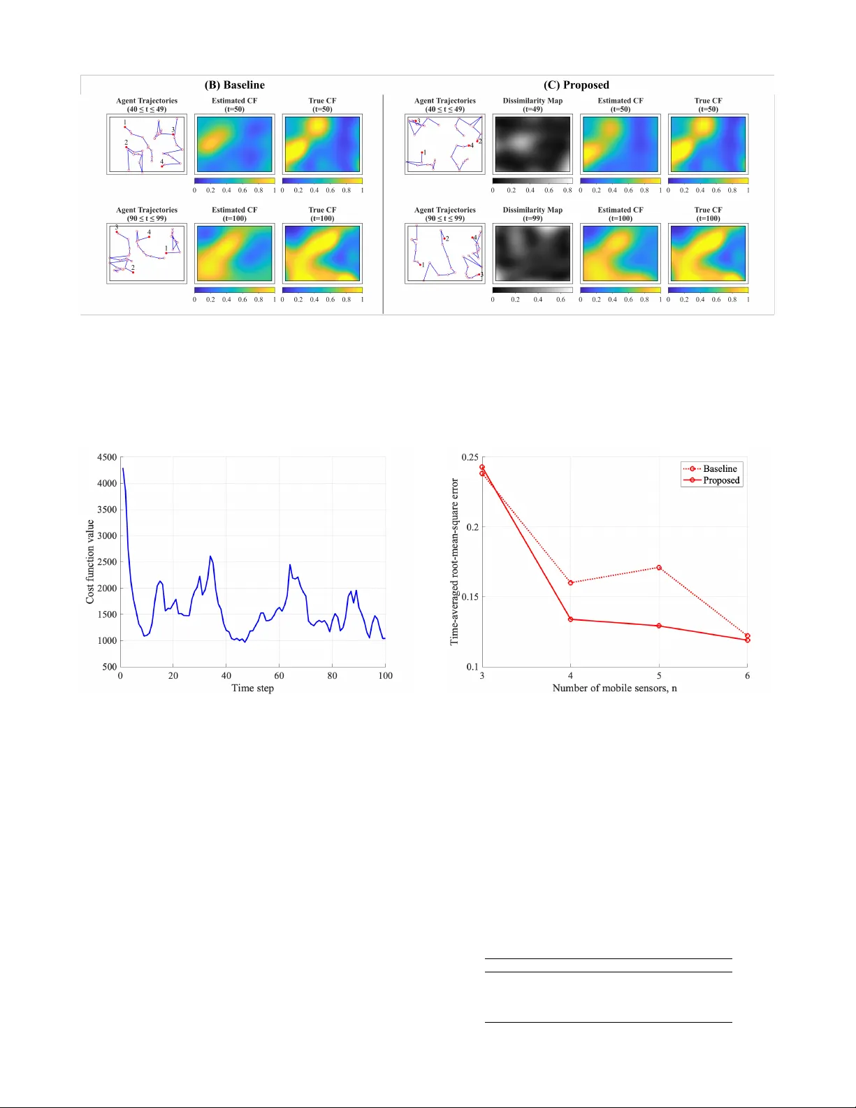
Dissimilarity-Based P ersistent Cov erage Contr ol of Multi-Robot Systems f or Impr oving Solar Irradiance Pr ediction Accuracy in Solar Thermal P ower Plants Haruki Kaw ase 1 , T aiga Suga wara 1 , and A. Daniel Carnerero 1 Abstract — Accurate for ecasting of future solar irradiance is essential for the effective control of solar thermal power plants. Although various kriging-based methods have been proposed to address the prediction problem, these methods typically do not provide an appropriate sampling strategy to dynamically position mobile sensors for optimizing prediction accuracy in real time, which is critical for achieving accurate for ecasts with a minimal number of sensors. This paper introduces a dissimilarity map derived fr om a kriging model and pro- poses a persistent coverage control algorithm that effectively guides agents toward regions wher e additional observations are r equired to impr ove pr ediction performance. By means of experiments using mobile robots, the proposed approach was shown to obtain more accurate predictions than the considered baselines under v arious emulated irradiance fields. Index T erms — Persistent Coverage Control, Robotic Sensor Networks, Solar Irradiance F orecasting, Dissimilarity Func- tions, Kriging I . I N T R O D U C T I O N Solar energy has attracted considerable attention as a major rene wable energy source. Representative technologies include photov oltaic (PV) po wer generation and concentrated solar thermal (CST) po wer generation. The levelized cost of electricity (LCOE) of PV plants is significantly lower than that of CST plants [1]. Nev ertheless, CST plants offer a critical advantage in that thermal energy storage (TES) enables electricity generation during nighttime hours [1]. Among CST technologies, solar tower and parabolic trough systems are the most prev alent. In solar to wer plants, hun- dreds to thousands of heliostats reflect sunlight toward a central receiver mounted on a tower , where a heat transfer fluid (HTF) is heated. In parabolic trough plants, parabolic mirrors concentrate sunlight onto a receiv er tube, heating an HTF such as oil that flows through the tube. In parabolic trough plants, the HTF flow rate must be controlled to maximize po wer generation while keeping the HTF temperature within operational limits. Model Predictiv e Control (MPC) is a propitious control strategy for this task [2], as it can explicitly handle constraints while computing optimal control inputs. Such MPC-based control requires accurate predictions of the spatial distribution of direct normal irradiance (DNI). If the HTF flo w is not appropriately controlled, parts of the plant may experience o verheating or 1 Graduate School of Engineering Science, The University of Osaka, Osaka, Japan. kawase.haruki.5or@ecs.osaka-u.ac.jp, sugawara.taiga.xxe@ecs.osaka-u.ac.jp, carnerero.daniel.es@osaka-u.ac.jp insufficient heating, resulting in inefficient use of solar en- ergy [3]. Consequently , accurate short-term DNI forecasting is essential for the optimal operation of parabolic trough CST plants. DNI losses are often quantified using the cloud factor (CF), a scalar variable taking values between 0 and 1, where 1 corresponds to complete DNI loss and 0 represents nominal DNI [3]. Kriging has become a de facto standard technique for spa- tial prediction based on limited observations [1], [4]. Kriging interpolates spatial data by estimating covariance structures through variogram models and computing weighted averages of observed values [5], [6]. Numerous studies have extended kriging to spatio-temporal settings [7], [8], and anisotropic spatio-temporal variograms that depend on wind effects have been shown to impro ve solar irradiance prediction accuracy [1]. Howe ver , prediction models that incorporate anisotropy tend to be complex and require ad-hoc treatments. T o ad- dress this, Kriging using dissimilarity functions has been studied in [9], as it allows for easier model construction and expansion. Kernel-Based Kriging (KB-Kriging) [10] is a representative example of this class of approaches for irradiance prediction, and improves prediction accuracy by sufficiently utilizing historical observation data. Nev erthe- less, the authors consider fixed sensor placement, which limits prediction performance. This is because fixed sensors can only observe spatially limited solar irradiance, making it difficult to detect a spatially non-uniform DNI distribution across the plant. Therefore, appropriate sampling strategies need to be developed so that accurate prediction can be carried out with a minimal number of sensors. This motiv ates the use of mobile robotic sensor networks (RSNs) [3]. Field estimation with RSNs is closely related to adaptiv e sampling, and Gaussian processes (GPs) are frequently employed [11], [12]. In particular, the method in [12] incorporates GP-based prediction uncertainty into a coverage control algorithm to enhance the estimation of time-varying processes. While coverage control is a standard approach for deploying multi-agent RSNs [13], it aims at con vergence to static optimal positions, thereby failing to fully exploit agent mobility for continuous monitoring tasks. T o address this limitation, persistent cov erage control has been studied in [14]–[16], where agents continuously mov e to monitor the en vironment. This is particularly important for solar irradiance forecasting, since cloud formations are highly dynamic and spatially complex. This study aims to develop control laws for mobile sensors that are applicable to a KB-Kriging predictor to improve irradiance prediction. W e consider a persistent monitoring problem in a parabolic trough CST plant in which multi- ple mobile agents continuously monitor a two-dimensional spatial domain. For the con venience of model construction in KB-Kriging, we propose a control framework in which the dissimilarity of KB-Kriging is fed back into the control laws of all agents. T o achieve this, we first define a KB- Kriging model for solar irradiance prediction using a dis- similarity function. Next, we introduce a dissimilarity map that represents how dissimilar a prediction point is from the observed data, and incorporate this map to define a time- varying importance function. Based on the map, we then design a persistent coverage controller for mobile agents. The effecti veness of the proposed method is demonstrated through experiments using mobile robots under virtual irra- diance fields. First, we implement solar irradiance prediction under cloudy conditions, comparing three methods: fixed sensors, a baseline persistent coverage control without the dissimilarity map, and the proposed method. Second, addi- tional experiments are conducted by changing the number of agents and climate conditions to ev aluate the performance of the proposed algorithm. The remainder of this paper is organized as follows. Sec- tion II describes the plant model and problem formulation. Section III introduces dissimilarity-based solar irradiance prediction. Section IV presents the proposed persistent co ver - age control strategy . Section V provides experimental results, and Section VI concludes the paper . I I . P R O B L E M F O R M U L A T I O N Let q = [ q 1 , q 2 ] ⊤ ∈ Q denote a vector representing a position in the plant. Here, Q ⊂ R 2 is a closed region representing the plant area and is the mission space over which solar irradiance is to be predicted. Let T ⊂ R be the time interval during which solar irradiance is observed and predicted, and denote time in this interval by t ∈ T . Fig. 1 illustrates the plant layout and a team of n robots sampling solar irradiance, where the robots are unmanned aerial vehicles (UA Vs) as representativ e sensing agents. The set of agents A i is defined as A = {A i | i ∈ I = { 1 , 2 , . . . , n }} (1) and let p i ( t ) ∈ Q denote the position of agent A i at time t . The spatio-temporal vector is defined as z q ,t = [ q ⊤ , t ] ⊤ = [ q 1 , q 2 , t ] ⊤ . The true solar irradiance at location q and time t is denoted by CF q ,t , and its predicted value by ˆ CF q ,t . It is necessary to search for the agents’ sampling locations that minimize E = 1 t T − t 0 Z t T t 0 RMSE( t ) dt, (2) where RMSE( t ) = s 1 |Q| Z Q    CF q ,t − ˆ CF q ,t    2 dq . (3) Fig. 1. Layout of the plant and spatio-temporal sampling locations of n robots Here, t 0 and t T denote the start and end times of the prediction ev aluation, respectiv ely , and |Q| denotes the area of the region Q . Problems of this type are typically NP-hard [17], and direct minimization of E is not straightforward. Therefore, we consider a persistent monitoring problem in which an importance function ϕ ( q , t ) : Q × R → [0 , ∞ ] for persistent cov erage control [14] is designed to minimize E . I I I . F U T U R E I R R A D I A N C E P R E D I C T I O N U S I N G D I S S I M I L A R I T Y F U N C T I O N S A. Dissimilarity Function A dissimilarity function quantifies how dissimilar a given element is from a prescribed dataset. Let ¯ d i ∈ R n d denote a sampled data point, and define the dataset as follows. D =  ¯ d 1 , . . . , ¯ d N  ∈ R n d × N (4) W e consider how dissimilar an arbitrary vector d ∈ R n d is with respect to this dataset. Here, n d denotes the data dimension and N the number of sampled data points. The dissimilarity function is defined as J : R n d × R n d × N → [0 , ∞ ] . A larger value of the dissimilarity function J ( d, D ) indicates that d is less similar to the dataset D , whereas a smaller value indicates higher similarity . A dissimilarity function that is in variant under affine transformations and independent of the coordinate system is given by the follow- ing formulation [9]: J γ ( d, D ) = min λ 1 ,...,λ N (1 − γ ) N X i =1 w i λ 2 i + γ N X i =1 | λ i | (5a) s.t.  D 1 ⊤  λ =  d 1  (5b) This is a con ve x optimization problem and can be solved efficiently with equality constraints. λ = [ λ 1 , . . . , λ N ] ⊤ ∈ R N is a weight vector , and γ ∈ [0 , 1) is a tuning parameter . The constants w i ( i = 1 , . . . , N ) are weighting coefficients that allow dif ferent importance to be assigned to each data point in D . This weighting is particularly useful when incorporating local information in nonlinear system modeling [18]. B. K ernel-Based Kriging (KB-Kriging) W e explain Kernel-Based Kriging (KB-Kriging), which computes one-step-ahead prediction ˆ CF q ,t +1 using a dissim- ilarity function [10]. From the past L time steps up to time t , a total of N observ ations of CF are selected, and the observation dataset Y t ∈ R 1 × N is defined as Y t = [ ¯ CF p 1 , t − L +1 , . . . , ¯ CF p n , t − L +1 , . . . , ¯ CF p 1 , t , . . . , ¯ CF p n , t ] (6) In addition, the dataset consisting of the corresponding spatio-temporal vectors, arranged in the same order as Y t , is denoted by Z t ∈ R n z × N , where Z t = [ ¯ z 1 , . . . , ¯ z N ] . Here, n z denotes the dimension of the spatio-temporal vector , which is n z = 3 . This dataset is obtained by reinde xing Z t = [ ¯ z p 1 , t − L +1 , . . . , ¯ z p n , t − L +1 , . . . , ¯ z p 1 , t , . . . , ¯ z p n , t ] (7) Please note that the datasets change at every sampling instant. Next, a regressor corresponding to the spatial location and the prediction time is defined as z q ,t +1 = [ q 1 , q 2 , t + 1] ⊤ ∈ R n z . KB-Kriging employs kernel functions to flexibly represent nonlinear spatial distributions, while requiring the system matrices to be computed only once at each time step. In kernel methods, data with a nonlinear structure are mapped into a high-dimensional Hilbert space through nonlinear operators. Let φ ( · ) : R n z → H denote a nonlinear operator , and for simplicity denote φ z = φ ( z ) for z ∈ R n z . The predicted cloud factor can then be expressed as a weighted av erage of Y t : ˆ CF q ,t +1 = Y t λ ∗ q ,t , (8) where λ ∗ q ,t ∈ R N is the optimal weight vector . Formally , with φ Z t = [ φ ¯ z 1 , . . . , φ ¯ z N ] , and using the framework of the dissimilarity function (5) with γ = 0 for mathematical con ve- nience, λ ∗ q ,t is obtained by solving the follo wing optimization problem. λ ∗ q ,t = argmin λ q,t λ ⊤ q ,t H 1 λ q ,t +   φ Z t λ q ,t − φ z q,t +1   2 (9a) s.t. 1 ⊤ λ q ,t = 1 (9b) This problem is obtained by relaxing the linear constraint Z t λ = z q ,t +1 of Local-Data Kriging [19] and incorporating a kernel-based penalty function to capture nonlinear corre- lations. Here, H 1 is a weighting matrix and is defined as H 1 = β I N using the parameter β . Expanding the penalty function, the objectiv e function can be rewritten as 1 2 λ ⊤ q ,t H t λ q ,t + f ⊤ q ,t λ q ,t + 1 . (10) Follo wing [10], for any pair z , z ′ ∈ R n z , the inner product is defined as ⟨ φ z , φ z ′ ⟩ = φ ⊤ z φ z ′ , and the following Gaussian kernel with parameters σ and τ is employed: ⟨ φ z , φ z ′ ⟩ = exp  − ∥ q − q ′ ∥ 2 2 σ 2  · exp  − ∥ t − t ′ ∥ 2 2 τ 2  (11) Here, H t = 2  H 1 + φ ⊤ Z t φ Z t  and f ⊤ q ,t = − 2 φ ⊤ z q,t +1 φ Z t . The kernel-related terms are given by φ ⊤ Z t φ Z t =      ⟨ φ ¯ z 1 , φ ¯ z 1 ⟩ ⟨ φ ¯ z 1 , φ ¯ z 2 ⟩ . . . ⟨ φ ¯ z 1 , φ ¯ z N ⟩ ⟨ φ ¯ z 2 , φ ¯ z 1 ⟩ ⟨ φ ¯ z 2 , φ ¯ z 2 ⟩ . . . ⟨ φ ¯ z 2 , φ ¯ z N ⟩ . . . . . . . . . ⟨ φ ¯ z N , φ ¯ z 1 ⟩ ⟨ φ ¯ z N , φ ¯ z 2 ⟩ . . . ⟨ φ ¯ z N , φ ¯ z N ⟩      (12) φ ⊤ z q,t +1 φ Z t =   φ z q,t +1 , φ ¯ z 1   φ z q,t +1 , φ ¯ z 2  . . .  φ z q,t +1 , φ ¯ z N   (13) This kernel function assumes separability between spatial and temporal components, which implies that there are no spatial and temporal correlations. Also, this kernel function shows the best prediction accurac y for this particular problem in [10]. Although the spatio-temporal structure of the kernel can be reconsidered to further enhance accuracy , this study focuses on improving prediction performance through the sampling strategy . As a result, the dissimilarity function incorporating kernel functions, J φ : R n z × R n z × N → [0 , ∞ ] , is formulated as follows: J φ ( z q ,t +1 , Z t ) = min λ q,t 1 2 λ ⊤ q ,t H t λ q ,t + f ⊤ q ,t λ q ,t + 1 (14a) s.t. 1 ⊤ λ q ,t = 1 (14b) The optimal weight vector λ ∗ q ,t is the minimizer of (14). The predicted value is then given by ˆ CF q ,t +1 = Y t λ ∗ q ,t . (15) This dissimilarity function quantitativ ely measures the dis- similarity between the prediction re gressor z q ,t +1 and the observed dataset Z t in the feature space. I V . D I S S I M I L A R I T Y - B A S E D P E R S I S T E N T C O V E R AG E C O N T RO L In this section, based on the theory of persistent cov erage control with information decay [14], we propose a method for designing an importance function and a corresponding controller that are suitable for kriging-based prediction. A. Agent and Information Model a) Agent Model: Let u i ( t ) ∈ R 2 denote the control input applied to agent A i at time t . Each agent is assumed to follow the following kinematic model: ˙ p i ( t ) = u i ( t ) (16) The communication network among agents is assumed to be fully connected, such that information can be shared between any pair of agents A i and A j ( i, j ∈ I ) . b) Measur ement Function: The measurement function represents the sensing capability of an agent as a function of its position. Let r and C denote the sensing radius and a positiv e constant, respectively , and define s i = ∥ q − p i ( t ) ∥ 2 . The measurement function is defined as M i ( s i ) =    C r 4 ( s i − r 2 ) 2 , if s i ≤ r 2 , 0 , if s i > r 2 . (17) The measurement map is defined as the sum of the measure- ment functions of all agents: M ( s ) = X i ∈I M i ( s i ) , (18) where s denotes the set of all s i . c) Information Model: The information map is defined as I ( q , t ) : Q × R → R + . The information dynamics are described by the following differential equation using a decay coefficient δ ≤ 0 : ∂ ∂ t I ( q , t ) = δ I ( q , t ) + M ( s ) . (19) The first term represents natural information decay , while the second term represents information acquisition based on the measurement map. Information increases in regions close to the agents and decreases elsewhere. Let I ref ( q ) denote the desired information lev el over the field. The agents are expected to mov e persistently to achie ve the desired information lev el at all locations. B. Importance Function Based on Dissimilarity Map Let ϕ ( q , t ) : Q × R → [0 , ∞ ] denote a time-varying function that represents the importance of location q at time t . This function is used to manage regions of interest for monitoring. In this study , dissimilarity information is incorporated into the importance function design. Specifi- cally , an importance function dependent on the dataset Z t is constructed as ϕ Z t ( q , t ) = J φ ( z q ,t +1 , Z t ) , (20) which is referred to as the dissimilarity map. Consequently , regions with high kriging dissimilarity are assigned higher importance values. The dissimilarity map is constructed online in a centralized manner based on Section III-B. C. Contr ol Objective The control objectiv e is to persistently move the agents such that no region in the mission space Q remains uncov- ered within the sensing domain, with particular emphasis on re gions exhibiting high dissimilarity . Let e I = I ref ( q ) − I ( q , t ) denote the information error, and define the informa- tion penalty function as h ( e I ) =  max(0 , e I )  2 . Then, the objectiv e function to be minimized is given by min H ( t ) = Z Q h ( e I ) ϕ Z t ( q , t ) dq . (21) D. Dissimilarity-Based P ersistent Covera ge Control Follo wing [14], we propose the following controller to achiev e the control objective: u i ( t ) = − k Z q ∈S i h ′ ( e I ) M ′ ( s i )( q − p i ) ϕ Z t ( q , t ) dq , (22) where S i ( p i ( t )) = { q ∈ Q | ∥ q − p i ( t ) ∥ ≤ r } denotes the sensing region, h ′ ( e I ) = max(0 , 2 e I ) , and k ∈ R + is a control gain. If the information lev el within the sensing region exceeds the desired lev el and no penalty is present, the control input giv en in (22) becomes zero. This condition can be expressed as I ≥ I ref ∀ q ∈ S i ⇒ h ′ = 0 ∀ q ∈ S i ⇒ u i ( t ) = 0 . When the above condition holds, an alternative controller is employed. Let ˆ k ∈ R + denote a control gain, and let ˆ q i be an arbitrary point within the sensing region S i . The controller is defined as ˆ u i ( t ) = − ˆ k ( p i ( t ) − ˆ q i ) . (23) T o simplify , let us denote the control law in this manner: u ∗ i ( t ) = ( u i ( t ) , if h ′  = 0 for some q ∈ S i , ˆ u i ( t ) , if h ′ = 0 ∀ q ∈ S i . (24) For a sufficiently large gain k such that ∂ ϕ Z t ∂ t ( q , t ) ≪ k and ∂ 2 ϕ Z t ∂ t 2 ( q , t ) ≪ k , an analysis can be performed to establish the boundedness of the objective function. Under these conditions, it has been shown that the controller u i ( t ) keeps the objecti ve function H ( t ) bounded as 0 ≤ H ( t ) ≤ ¯ H for a positiv e constant ¯ H [14]. V . E X P E R I M E N TA L R E S U L T S A. Experimental V alidation In this section, experimental results of one-step-ahead solar irradiance prediction over the mission space Q using a KB-Kriging predictor are presented, comparing three meth- ods: (A) a fixed sensor deployment, (B) a baseline persistent cov erage control method with ϕ ( q , t ) = 1 , and (C) the proposed method. Whereas prediction using (A) the fixed method is conducted entirely in MA TLAB, (B) and (C) are implemented in a hardware-in-the-loop configuration using T urtleBot3 to provide a proof of concept. See [21] for the specifications of T urtleBot3. Although the proposed algo- rithm is formulated for holonomic systems such as U A Vs, it remains effecti ve for nonholonomic systems like T urtleBot3 because the computed control input is used as a high-lev el reference input for a low-le vel controller . The number of agents is n = 4 , and we set the prediction interval from t 0 = 1 to t T = 100 . Prediction is performed sequentially for each time step t ∈ { 1 , 2 , . . . , 100 } based on data available at t − 1 . A PC with Ubuntu 20.04 equipped with intel Core i7 CPU, an NVIDIA GeForce GTX 1650 Mobile/Max-Q, and 16 GB of RAM was used, and T urtleBot3 was controlled using R OS Noetic. Regarding (A), assuming a uniform importance distribu- tion over the mission space Q , the fixed sensor positions are set to the centroids of the V oronoi regions computed using Lloyd’ s algorithm. The fixed sensor configurations and initial mobile agent positions are summarized in T able I. W e use the cloudy-condition solar irradiance dataset over Q provided by J. G. Martin et al. [1]. The dataset consists of a 97 × 72 spatial grid and 2000 time steps. The mission space Q is q 1 ∈ [ − 1 . 41 , 2 . 38] , q 2 ∈ [ − 1 . 26 , 1 . 53] [m], and is discretized into a 97 × 72 grid according to the dataset shape. Continuous spatial integrals are approximated by discrete summation. Note that irradiance measurements can only be obtained at the agent position p i ( t ) regardless of r . T able II summarizes the key experimental settings, and the layout of the experiment room can be seen in Fig. 2. Self-localization is performed using odometry , and coor- dinate frame transformations are managed by the ROS tf library . Pose information is obtained at a frequency of 60 Hz, and the maximum velocity and acceleration of the robots are limited to 0.15 m/s and 0.1 m/s 2 , respectiv ely . Algorithm 1 summarizes the computation of the next sampling locations and velocity commands of the robots. At each time step, a virtual input u ∗ i ( t ) is calculated according to (24). The next target position p next i is periodically updated as p next i = p i ( t ) + u ∗ i ( t ) , and is distributed from the goal node via the R OS topic communication ( /tb3 i/goal ). Let p r i = p next i − p i denote the deviation between the current position and the next position. In addition, let θ i and θ next i be the current and the desired heading angle of robot i to the next location, respectively . The angular deviation is defined as θ r i = θ next i − θ i . T o guide the robot to ward the next target position, the linear and angular velocity inputs v i , ω i are determined by the following control la ws: v i = K p p r i , ω i = ( K ω θ r i , v i > 0 , − K ω θ r i , v i ≤ 0 , (25) where K p = 0 . 8 and K ω = 1 . 0 . The update of the next sampling location p next i is ex ecuted ev ery 8 s, whereas the velocity commands v i ( · ) and ω i ( · ) are transmitted at 10 Hz via a wireless LAN router using the most recently receiv ed target position. In case the robots come close to each Fig. 2. Layout of the experiment room and the initial configurations of 4 mobile agents. Algorithm 1: Computation of sampling locations and control inputs Initialize p i (0) for all i ∈ I ; for t = 0 , 1 , 2 , . . . , t T − 1 do // Path planning and prediction step (every 8 s) for each robot i ∈ I do Compute reference input u ∗ i ( t ) in (24); p next i ← p i ( t ) + u ∗ i ( t ) ; Publish p next i via R OS topic /tb3 i/goal ; while receiving p next i do // Control loop (10 Hz) Obtain current pose p i and θ i by odometry; p r i ← p next i − p i ; θ r i ← θ next i − θ i ; Compute v i and ω i in (25) and send them to robot; other , collision av oidance is implemented by incorporating a repulsiv e function into the velocity commands. Note that the solar irradiance observations are obtained from a virtual en vironment for (B) and (C). Although the typical forecasting cycle for solar irradiance in solar thermal po wer plants ranges from 60 s to 300 s [1], the update interval of 8 s is adopted here for experimental validation and does not aim to reflect an actual operational forecasting cycle. The tuning parameters are β , σ, τ for (A), and k , ˆ k , β , σ, τ , δ for (B) and (C). These parameters are opti- mized using MA TLAB’ s fmincon to minimize E in (2), using 100 data points from the first half of the dataset. The tuning results are summarized in T able III. For prediction accuracy ev aluation, another 100 data points extracted from the second half of the dataset are used. Fig. 3 shows the time-series RMSE for each method. (C) maintains lo wer RMSE than the other methods at almost all time steps, confirming improved accurac y . As shown in T able IV, the time-av eraged RMSE E for the fixed, baseline, and proposed methods indicates that (C) achiev es the best performance. Experiment videos are av ailable here. T ABLE I C O NFI G U R A T I O NS O F FI XE D SE N S O RS A ND M OB I L E AG E N T S F ixed sensor configuration Sensor positions (V oronoi centroids) p 1 = (1 . 42 , 0 . 84) p 2 = (1 . 45 , − 0 . 57) p 3 = ( − 0 . 45 , − 0 . 57) p 4 = ( − 0 . 48 , 0 . 84) Mobile agent configuration Initial positions p 1 (0) = ( − 0 . 54 , − 0 . 54) p 2 (0) = ( − 0 . 54 , 0 . 86) p 3 (0) = (0 . 86 , − 0 . 52) p 4 (0) = (0 . 80 , 0 . 86) Fig. 3. Time-series RMSE comparison (n=4) among (A) the fix ed method, (B) the baseline method, and (C) the proposed method. In (A), the coordinate information of Z t stored in the dataset is fixed over time, and accordingly , the observations in Y t are limited to solar irradiance data at those fixed coor- dinates. When predicting the solar irradiance at an arbitrary coordinate q using the regressor z q ,t +1 = [ q 1 , q 2 , t + 1] ⊤ , the predicted value is given by ˆ CF q ,t +1 = Y t λ ∗ according to (15). Howe ver , if the prediction point q is far from the observed coordinates in Z t in feature space, there are many prediction points that lie outside the conv ex hull defined by the observations. This leads to a large dissimilarity value and degraded prediction performance. Conv ersely , if q lies near one of the coordinates in Z t in the feature space, neighboring information can be exploited, resulting in predictions with smaller dissimilarity . Therefore, in (A), predictions with large dissimilarity dominate in regions without sensor placement, T ABLE II E X PE R I M EN TA L S ET T I N GS Item Setting Q − 1 . 41 ≤ q 1 ≤ 2 . 38 − 1 . 26 ≤ q 2 ≤ 1 . 53 (97 × 72 grid ) L 10 t 0 , t T 1,100 n 4 C 0.3 r 0.5 Observation noise Not considered Initial information map I ( q , 0) = 0 ∀ q Reference information map I ref ( q ) = 1 ∀ q ∈ Q T ABLE III T U NI N G PA R AM E T ER S Parameter (A) Fixed (B) Baseline (C) Proposed β 0.0003665 0.211844 0.169103 σ 0.297397 0.166996 0.202815 τ 0.119574 0.303474 0.329897 k – 0.016427 0.057800 ˆ k – 0.268257 0.399603 δ – -0.138640 -0.209257 T ABLE IV E R RO R C O MPA R IS O N ( n = 4 ) U N D E R C L OU DY WE ATH E R (A) Fixed (B) Baseline (C) Proposed E 0.235 0.160 0 . 134 leading to inferior prediction accuracy compared to the other methods. Fig. 4 compares the estimation performance between (B) and (C), including the agent trajectories for both methods ov er two time intervals. In (B), the agents continuously change sampling locations, causing spatial div ersity in the coordinates of Z t and the corresponding observ ations Y t . This increases the likelihood of having nearby observ ations for kriging at arbitrary locations, reducing highly dissimilar predictions compared to (A). Howe ver , because (B) aims to monitor the entire Q , at certain times, the agents may cluster in similar regions or explore areas where they hav e already sampled data. This implies that kriging in unvisited regions relies strongly on highly dissimilar estimates. In contrast, (C) incorporates regions of high dissimilarity into the sampling decision, driving the agents to mov e in a way that suppresses the overall dissimilarity map. As a result, the con vex hull characterized by the observed data is expanded, prev enting highly dissimilar predictions from dominating solar irradiance estimation across the field. Fig. 5 presents the time evolution of the objectiv e function H ( t ) for (C). The v alues remain bounded, indicating the stability of the control law . This shows that when dissim- ilarity increases in regions far from observation points, the agents move to ward those regions to reduce dissimilarity . For confirmation, the first- and second-order time deriv ati ves of the dissimilarity map in (C) were numerically approximated. As a result, max t max q    ∂ ϕ Z t ∂ t ( q , t )    ≈ 1 . 93 × 10 − 4 ≪ k , max t max q    ∂ 2 ϕ Z t ∂ t 2 ( q , t )    ≈ 2 . 88 × 10 − 5 ≪ k , confirming that the necessary assumptions for demonstrating the bound- edness of the objectiv e function are satisfied. B. P erformance Evaluation T o further ev aluate the performance of (C), solar irradi- ance prediction under cloudy conditions is conducted with n = 3 , 5 , 6 agents. W e reuse the tuning parameters shown in T able III. Initial agent positions are randomly selected within the rectangular region q 1 ∈ [ − 0 . 54 , 0 . 80] , q 2 ∈ [ − 0 . 54 , 0 . 86] . All other conditions are identical to those in Section V -A. The comparison method is (B) the baseline persistent cov erage control. As sho wn in Fig. 6, e xcept for the case n = 3 , (C) achie ves higher prediction accuracy than (B). For both methods, pre- diction accuracy tends to improv e as the number of sensors increases, since more sampling locations become av ailable. Howe ver , increasing the number of agents introduces trade- offs with system scalability and sensor deployment costs, which are left for future work. When n = 3 , no significant difference is observed between (B) and (C). This is attributed to the extremely limited number of agents and historical data Fig. 4. Comparison of the estimation performance between (B) the baseline method (left) and (C) the proposed method (right) corresponding to different time steps (top: t = 50 and bottom: t = 100 ). The inner rectangle represents the region Q , while the outer rectangle indicates the area extended by 30 cm both horizontally and vertically . The horizontal axis corresponds to q 1 , and the vertical axis corresponds to q 2 . Regarding the agent trajectories (blue lines), open red circles denote past sampling points, and filled red circles indicate the current agent positions. A total of n × L = 4 × 10 = 40 points are sampled in each field. Agents sometimes appear outside the region Q , which is due to localization errors. (C) incorporates the dissimilarity map into sampling strategies, leading to lower error compared with (B). Fig. 5. Time-series evolution of the objective function value in (C) the proposed method. relativ e to the large observation area, resulting in uniformly high dissimilarity and making the adaptiv e sampling inef- fectiv e. When n = 6 , the performance gap narrows because the prediction accuracy saturates with a sufficient number of agents. T o ev aluate robustness against climate variation, solar irra- diance prediction is performed under three additional weather conditions (standard, sunny , very cloudy) in addition to the cloudy weather . The parameters in T able III are used again, and all other conditions remain the same as in Section V - A. As sho wn in T able V, the prediction accuracy of (C) outperforms that of (B) under all weather conditions. This demonstrates that (C) consistently improves solar irradiance prediction accuracy across varying climates, indicating that the proposed sampling strategy is generic, and ev en if the Fig. 6. Prediction accuracy with respect to the number of mobile sensors. weather changes, we do not need to tune the parameters again. V I . C O N C L U S I O N S In this study , we designed a novel controller that incor- porates the dissimilarity map into the importance function of persistent co verage control to improve solar irradiance T ABLE V P R ED I C T IO N A C CU R AC Y U N D ER D IFF E R E NT W EAT HE R CO N D I TI O N S ( n = 4 ) W eather (B) Baseline E (C) Proposed E standard 0.156 0.142 sunny 0.166 0.120 cloudy 0.160 0.134 very cloudy 0.144 0.125 prediction accuracy in concentrated solar thermal (CST) power plants. The proposed method determines the sampling locations of mobile sensors in an adapti ve way , thereby fully exploiting the capability of the KB-Kriging predic- tor . Experimental results using real robots demonstrate that the proposed method significantly reduces prediction errors compared with fix ed sensor configurations and the baseline persistent cov erage control. Howe ver , the size of commercial CST plants can be up to 780 ha [22], and communication connecti vity among agents cannot always be guaranteed. Moreov er , centralized computation poses scalability issues. Therefore, future work needs to focus on dev eloping a distributed framework for both prediction and construction of the dissimilarity map, which are currently performed in a centralized manner . A C K N O W L E D G M E N T The solar irradiance datasets used in this study were provided by J. G. Martin and J. M. Maestre. The authors are indebted to both researchers for generously providing the datasets. R E F E R E N C E S [1] J. G. Martin, J. R. D. Frejo, J. M. Maestre, and E. F . Camacho, “Spatio-temporal kriging for spatial irradiance estimation with short- term forecasting in a thermosolar power plant, ” Heliyon , vol. 10, no. 20, Art. no. e39247, 2024, doi: 10.1016/j.heliyon.2024.e39247. [2] J. R. D. Frejo and E. F . Camacho, “Centralized and distributed model predictiv e control for the maximization of the thermal power of solar parabolic-trough plants, ” Solar Energy , vol. 204, pp. 190–199, 2020, doi: 10.1016/j.solener .2020.04.033. [3] J. G. Martin, J. M. Maestre, and E. F . Camacho, “Spatial irradi- ance estimation in a thermosolar power plant by a mobile robot sensor network, ” Solar Energy , vol. 220, pp. 735–744, 2021, doi: 10.1016/j.solener .2021.03.038. [4] V . Roy , A. Simonetto, and G. Leus, “Spatio-temporal field estimation using kriged Kalman filter (KKF) with sparsity-enforcing sensor placement, ” Sensors , vol. 18, no. 6, Art. no. 1778, Jun. 2018, doi: 10.3390/s18061778. [5] H. Miura, “Spatio-temporal kriging-based estimation of urban au- tomobile tra vel time using probe-taxi data, ” Journal of the City Planning Institute of Japan , vol. 44, no. 3, pp. 793–798, 2009, doi: 10.11361/journalcpij.44.3.793. [6] N. Cressie, “The origins of kriging, ” Mathematical Geology , vol. 22, no. 3, pp. 239–252, 1990, doi: 10.1007/BF00889887. [7] N. Cressie and H.-C. Huang, “Classes of nonseparable, spatio- temporal stationary cov ariance functions, ” Journal of the American Statistical Association , vol. 94, no. 448, pp. 1330–1340, 1999, doi: 10.1080/01621459.1999.10473818. [8] T . Gneiting, “Nonseparable, stationary cov ariance functions for space– time data, ” Journal of the American Statistical Association , vol. 97, no. 458, pp. 590–600, 2002, doi: 10.1198/016214502760047113. [9] A. D. Carnerero, D. R. Ram ´ ırez, S. Lucia, and T . Alamo, “Prediction regions based on dissimilarity functions, ” ISA T ransactions , vol. 139, pp. 49–59, 2023, doi: 10.1016/j.isatra.2023.03.048. [10] N. Y uda and A. D. Carnerero, “Kernel-based kriging model for solar irradiance forecasting in solar thermal power plants, ” in Pr oceedings of the 25th Annual Conference of the Society of Instrument and Contr ol Engineers (SICE) , Kobe, Japan, May 2025, pp. 868–872, doi: 10.11509/sci.sci25.0 868. [11] T . Salam and M. A. Hsieh, “ Adaptive sampling and reduced-order modeling of dynamic processes by robot teams, ” IEEE Robotics and Automation Letters , v ol. 4, no. 2, pp. 477–484, Apr . 2019, doi: 10.1109/LRA.2019.2891475. [12] F . Pratissoli, M. Mantov ani, A. Prorok, and L. Sabattini, “Dis- tributed coverage control for time-varying spatial processes, ” IEEE T ransactions on Robotics , vol. 41, pp. 1602–1617, 2025, doi: 10.1109/TR O.2025.3539168. [13] J. Cortes, S. Martinez, T . Karatas and F . Bullo, ”Cov erage control for mobile sensing networks, ” in IEEE Transactions on Robotics and Automation, vol. 20, no. 2, pp. 243–255, April 2004, doi: 10.1109/TRA.2004.824698. [14] N. H ¨ ubel, S. Hirche, A. Gusrialdi, T . Hatanaka, M. Fujita, and O. Sawodn y , “Coverage control with information decay in dynamic en vironments, ” IF AC Pr oceedings V olumes , vol. 41, no. 2, pp. 4180– 4185, 2008, doi: 10.3182/20080706-5-KR-1001.00703. [15] Z. Lu, S. Y amashita, J. Y amauchi, and T . Hatanaka, “Distributed online assignment of charging stations in persistent coverage control tasks based on LP relaxation and ADMM, ” SICE Journal of Contr ol, Measur ement, and System Inte gration , vol. 15, no. 2, pp. 191–200, 2022, doi: 10.1080/18824889.2022.2125246. [16] X. Xu, E. Rodr ´ ıguez-Seda, and Y . Diaz-Mercado, “Persistent awareness-based multi-robot cov erage control, ” in Pr oc. 59th IEEE Conf. Decision and Control (CDC) , 2020, pp. 5315–5320, doi: 10.1109/CDC42340.2020.9304483. [17] K. Jakkala and S. Akella, “Multi-robot informative path planning from regression with sparse Gaussian processes, ” in Proc. IEEE Int. Conf. Robotics and Automation (ICRA) , Y okohama, Japan, 2024, pp. 12382– 12388, doi: 10.1109/ICRA57147.2024.10610484. [18] A. D. Carnerero, D. R. Ram ´ ırez, and T . Alamo, “Probabilistic in- terval predictor based on dissimilarity functions, ” IEEE T ransactions on Automatic Contr ol , vol. 67, no. 12, pp. 6842–6849, 2020, doi: 10.1109/T AC.2021.3136137. [19] A. D. Carnerero, D. R. Ram ´ ırez, and T . Alamo, “State-space krig- ing: A data-driv en method to forecast nonlinear dynamical systems, ” IEEE Contr ol Systems Letters , vol. 6, pp. 2258–2263, 2022, doi: 10.1109/LCSYS.2021.3140167. [20] A. D. Carnerero, D. R. Ram ´ ırez, D. Lim ´ on, and T . Alamo, “Kernel- based state-space kriging for predictiv e control, ” IEEE/CAA Journal of Automatica Sinica , vol. 10, no. 5, pp. 1263–1275, May 2023, doi: 10.1109/J AS.2023.123459. [21] Open Source Robotics Foundation, Inc. (2026). TurtleBot. Accessed: Jan. 21, 2026. [Online]. A v ailable: https://www .turtlebot.com/ [22] J. M. Aguilar-L ´ opez, R. A. Garc ´ ıa, A. J. S ´ anchez, A. J. Gallego, and E. F . Camacho, “Mobile sensor for clouds shadow detection and direct normal irradiance estimation, ” Solar Energy , vol. 237, pp. 470–482, 2022, doi: 10.1016/j.solener.2021.12.032.