Reinforcement learning for quantum processes with memory

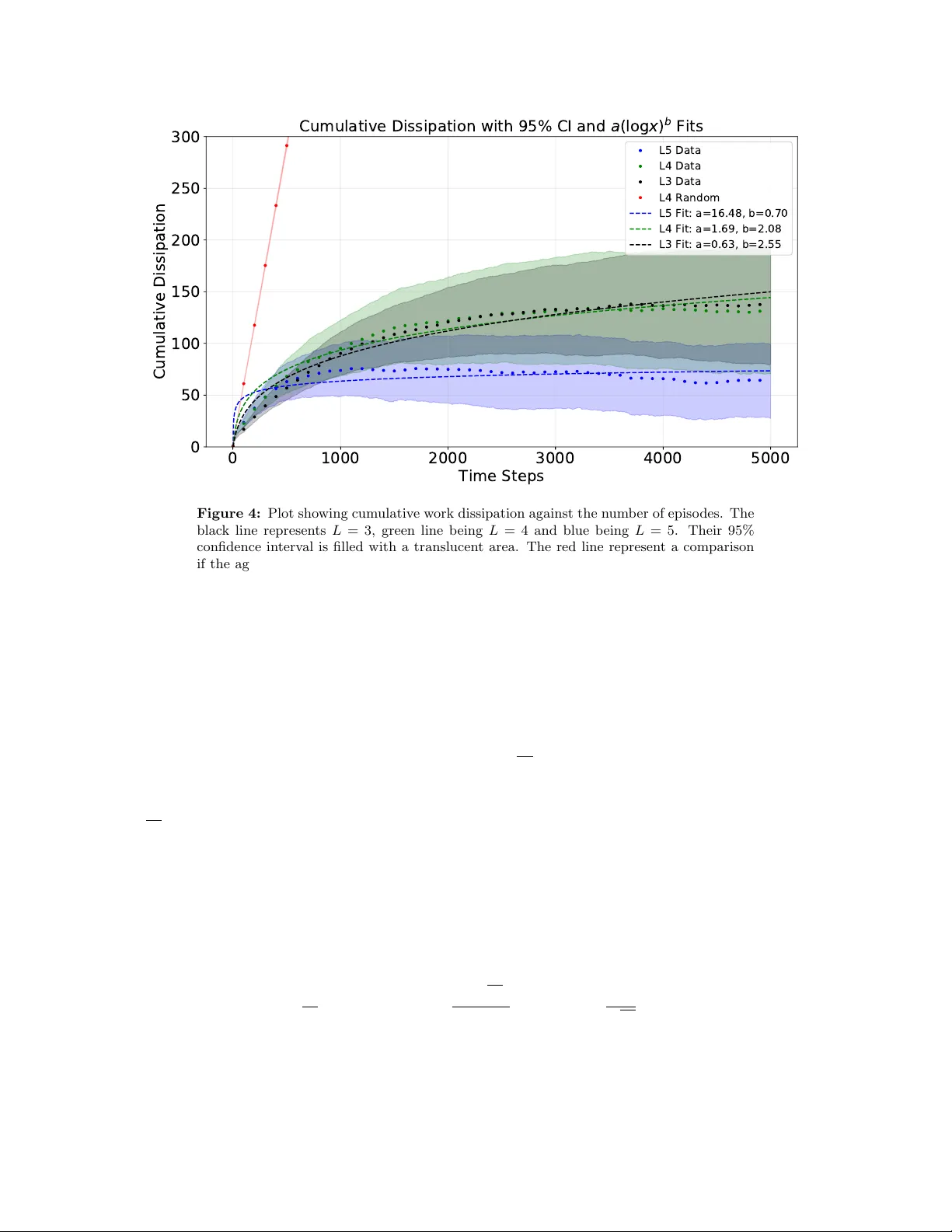
Reinforcemen t learning for quan tum pro cesses with memory Josep Lum breras * 1,2 josep.lz@n tu.edu.sg Ruo Cheng Huang * 1,2 ruo c heng001@e.n tu.edu.sg Y anglin Hu * 3 y anglin.hu@u.n us.edu Marco F anizza 4 marco.fanizza@inria.fr Mile Gu 1,2,5 mgu@quan tumcomplexity .org Marc h 27, 2026 Abstract In reinforcement learning, an agent interacts sequen tially with an environmen t to maximize a rew ard, receiving only partial, probabilistic feedbac k. This creates a fundamen tal exploration-exploitation trade-off: the agen t must explore to learn the hidden dynamics while exploiting this knowledge to maximize its target ob jective. While extensively studied classically , applying this framework to quan tum systems requires dealing with hidden quan tum states that ev olve via unknown dynamics. W e formalize this problem via a framework where the en vironmen t main tains a hidden quantum memory ev olving via unkno wn quantum c hannels, and the agent in tervenes sequentially using quantum instruments. F or this setting, we adapt an optimistic maximum-lik elihoo d estimation algorithm. W e extend the analysis to con tinuous action spaces, allowing us to model general p ositiv e op erator-v alued measures (PO VMs). By controlling the propagation of estimation errors through quan tum channels and instruments, we prov e that the cum ulative regret of our strategy scales as e O ( √ K ) o ver K episo des. F urthermore, via a reduction to the m ulti-armed quantum bandit problem, w e establish information-theoretic low er b ounds demonstrating that this sublinear scaling is strictly optimal up to poly- logarithmic factors. As a ph ysical application, w e consider state-agnostic work extraction. When extracting free energy from a sequence of non-i.i.d. quantum states correlated by a hidden memory , any lac k of kno wledge ab out the source leads to thermo dynamic dissipation. In our setting, the mathematical regret ex- actly quantifies this cum ulative dissipation. Using our adaptive algorithm, the agen t uses past energy outcomes to improv e its extraction proto col on the fly , ac hieving sublinear cumulativ e dissipation, and, consequen tly , an asymptotically zero dissipation rate. ∗ J. Lum breras, R. C. Huang, and Y. Hu contributed equally and share first authorship. 1 Nan yang Quantum Hub, School of Ph ysical and Mathematical Sciences, Nany ang T ec hnological Universit y , Singap ore 2 Cen tre for Quantum T ec hnologies, Nan yang T ec hnological Universit y , Singap ore 3 QICI Quan tum Information and Computation Initiativ e, School of Computing and Data Science, The Univ ersity of Hong Kong, Pokfulam Road, Hong Kong SAR, China 4 Inria, T´ el ´ ecom Paris - L TCI, Institut Polytec hnique de Paris 5 Ma juLab, CNRS-UNS-NUS-NTU International Joint Research Unit, UMI 3654, Singap ore 117543, Singap ore Con ten ts 1 In tro duction 3 1.1 Results . . . . . . . . . . . . . . . . . . . . . . . . . . . . . . . . . . . . . . . . . . . . 6 1.2 Discussion . . . . . . . . . . . . . . . . . . . . . . . . . . . . . . . . . . . . . . . . . . 14 1.3 Related W orks . . . . . . . . . . . . . . . . . . . . . . . . . . . . . . . . . . . . . . . 16 2 Quan tum Sto c hastic Pro cess F ramew ork 17 2.1 Notation . . . . . . . . . . . . . . . . . . . . . . . . . . . . . . . . . . . . . . . . . . . 17 2.2 Input-output QHMM environmen t . . . . . . . . . . . . . . . . . . . . . . . . . . . . 18 2.3 Sequen tial-emission HMM environmen t . . . . . . . . . . . . . . . . . . . . . . . . . . 19 2.4 P olicies . . . . . . . . . . . . . . . . . . . . . . . . . . . . . . . . . . . . . . . . . . . 20 2.5 Ob jectives . . . . . . . . . . . . . . . . . . . . . . . . . . . . . . . . . . . . . . . . . . 21 3 Observ able Operator Mo del 21 3.1 Undercomplete assumption . . . . . . . . . . . . . . . . . . . . . . . . . . . . . . . . 21 3.2 Observ able op erators . . . . . . . . . . . . . . . . . . . . . . . . . . . . . . . . . . . . 22 3.3 T ra jectory probabilities . . . . . . . . . . . . . . . . . . . . . . . . . . . . . . . . . . 23 4 Optimistic Maxim um Lik eliho o d Estimation for QHMMs 24 4.1 Em b edding dimension of the QHMM mo del class (discrete actions) . . . . . . . . . . 25 5 Regret analysis for discrete action spaces 27 5.1 Con trolling error propagation via quan tum recov ery maps . . . . . . . . . . . . . . . 27 5.2 Decomp osing regret via OOM estimation errors . . . . . . . . . . . . . . . . . . . . . 32 5.3 The eluder dimension for linear functions . . . . . . . . . . . . . . . . . . . . . . . . 33 5.4 Cum ulative regret bound for discrete actions . . . . . . . . . . . . . . . . . . . . . . 38 6 Extension to con tinuous action spaces 39 6.1 Con tinuous action setting . . . . . . . . . . . . . . . . . . . . . . . . . . . . . . . . . 39 6.2 Em b edding (spanning) dimension for contin uous actions . . . . . . . . . . . . . . . . 40 6.3 Undercomplete assumption and recov ery map for contin uous actions . . . . . . . . . 42 6.4 Concen tration b ounds for contin uous actions . . . . . . . . . . . . . . . . . . . . . . 45 6.5 Decomp osing regret via OOM estimation errors for contin uous actions . . . . . . . . 46 6.6 The eluder dimension for linear functions (con tinuous actions) . . . . . . . . . . . . . 47 6.7 Cum ulative regret bound for con tinuous actions . . . . . . . . . . . . . . . . . . . . . 52 7 Information-Theoretic Lo wer Bounds 54 7.1 The MAQB F ramew ork and SIC-POVMs . . . . . . . . . . . . . . . . . . . . . . . . 54 2 7.2 Regret Low er Bound via MA QB with SIC-POVMs . . . . . . . . . . . . . . . . . . . 55 7.3 Lo wer Bound for QHMMs via Reduction to MAQB . . . . . . . . . . . . . . . . . . . 57 7.4 Lo wer Bound for the Observ ability P arameter via Classical POMDPs . . . . . . . . 58 8 Application: State-agnostic quan tum w ork extraction 59 8.1 W ork extraction from sequential-emission HMM en vironments . . . . . . . . . . . . . 60 8.2 W ork-extraction and action-dep enden t rewards . . . . . . . . . . . . . . . . . . . . . 62 8.3 W ork extraction proto col . . . . . . . . . . . . . . . . . . . . . . . . . . . . . . . . . 64 8.4 Cum ulative dissipation as mathematical regret . . . . . . . . . . . . . . . . . . . . . 67 9 Numerical experiments 69 9.1 Computing optimal p olicy via dynamic programming . . . . . . . . . . . . . . . . . . 69 9.2 Case Study . . . . . . . . . . . . . . . . . . . . . . . . . . . . . . . . . . . . . . . . . 72 A Pro ofs for MLE concen tration bounds with con tinuous actions 79 A.1 T ra jectory densities and parameter space embedding . . . . . . . . . . . . . . . . . . 79 A.2 Optimistic brack eting and mas s inflation . . . . . . . . . . . . . . . . . . . . . . . . . 80 A.3 Pro of of Prop osition 6.7 (Lik eliho o d ratio concen tration) . . . . . . . . . . . . . . . . 81 A.4 Pro of of Prop osition 6.8 (T ra jectory ℓ 1 concen tration) . . . . . . . . . . . . . . . . . 82 B Detailed deriv ation for work distribution 84 1 In tro duction In reinforcemen t learning (RL), an agent in teracts sequentially with an unkno wn en vironment to learn optimal decision-making [ 69 ]. The primary mec hanism driving this learning pro cess is the maximization of a cum ulative rew ard signal, a versatile form ulation capable of enco ding complex tasks such as the con trol of autonomous rob ots [ 37 ], autonomous navigation [ 42 ], and industrial re- source optimization [ 54 , 52 ]. Ho w ever, in most realistic ph ysical settings, suc h as a robot na vigating a cluttered, partially mapp ed physical space, the agent lac ks direct access to the true underlying state of the system. Such scenarios are traditionally mo deled as Parti ally Observ able Mark ov De- cision Processes (POMDPs) [ 36 ]. This partial observ ability severely complicates learning, as the agen t m ust main tain a history of past interactions to infer the latent dynamics while sim ultaneously balancing the fundamental explor ation-exploitation tr ade-off . While the theoretical understanding of exploration in classical POMDPs has seen significan t recen t breakthroughs [ 35 , 44 ], these classical framew orks are fundamentally incompatible with quantum ph ysical systems. As quantum tec hnologies mature, there is a critical need for agen ts capable of learning and con trolling quantum pro cesses. Reinforcement learning has emerged as a highly effectiv e to ol for this task, demonstrating significan t success across several fundamental domains. In quan tum con trol and state preparation, RL agents ha v e b een deploy ed to discov er optimal control pulses and stabilize complex target states, frequen tly outp erforming traditional gradien t-based optimal con trol metho ds b y learning robust p olicies directly from en vironmen tal interaction [ 5 , 78 ]. In quan tum 3 circuit compilation, RL is utilized to autonomously generate hardware-efficien t gate sequences and routing strategies that minimize circuit depth and limit decoherence [ 61 ]. Most notably , RL has driv en massive breakthroughs in quantum error correction. While foundational w orks established the ability of RL to autonomously disco ver no v el error-correcting codes and decoding strategies [ 5 ], recen t landmark results by Go ogle Quantum AI ha ve repurp osed the error correction cycle itself as an RL en vironment [ 75 ]. By utilizing binary error detection ev ents as learning signals, these agents con tinuously tune thousands of ph ysical con trol parameters on the fly , activ ely stabilizing logical qubits against environmen tal drift. Despite these impressiv e application-sp ecific successes, learning and controlling general pro- cesses in these settings remains intrinsically difficult: unlik e classical probability distributions, hidden quan tum states ev olve via completely p ositiv e trace-preserving (CPTP) c hannels, and the agen t’s very act of gathering information inevitably disturbs the latent state. Consequently , the canonical reinforcement learning problem, where an agent sequen tially interacts with an unknown ev olving en vironment to maximize a cum ulative reward, lac ks a rigorous form ulation when the en vironment itself is quan tum. It is fundamentally natural to consider a classical agen t probing an ev olving quantum process to dynamically extract a contin uous resource (Figure 1 ). State-agnostic w ork extraction is a k ey example, whic h has b een successfully explored in the i.i.d. s etting [ 48 , 76 ]. Ho wev er, realistic physical sources rarely emit uncorrelated states. Instead, they exhibit temp oral correlations driven b y an inaccessible laten t memory . This necessitates a shift to the non-i.i.d. regime, where an agen t seeks to harvest thermodynamic free energy from a sequence of correlated quan tum states. In such settings, the agen t must contin ually balance learning the underlying emis- sion dynamics with maximizing its physical energy yield. This ph ysical scenario exemplifies the broader c hallenge of sequen tial rew ard maximization under unknown quantum dynamics, motiv at- ing our central question: Can a classic al agent efficiently r esolve the fundamental explor ation-exploitation tr ade-off over an unchar acterize d quantum sto chastic pr o c ess? T o rigorously formalize the problem of maximizing rewards ov er quantum processes, w e in- tro duce the input-output Quantum Hidden Markov Mo del (QHMM). This framew ork serv es as a true POMDP-style generalization for quantum systems, treating the laten t transition dynamics as strictly unkno wn and learned purely through in teraction. F urthermore, it acts as the natural, stateful extension of the Multi-Armed Quantum Bandit (MAQB) framew ork [ 47 ]. In our episo dic QHMM setting, the environmen t carries a finite-dimensional quantum memory that evolv es in time. A t each step, the agent probes the system by selecting an action corresp onding to a quantum in- strumen t, pro ducing a classical outcome (reward) and a corresp onding post-measurement memory state. While the QHMM faithfully captures the memory of the quantum process, learning and con- trolling its dynamics directly p oses a fundamental challenge: the underlying quan tum state driving this memory is inherently unobserv able. T o ov ercome this limitation, we adopt the framew ork of Observ able Operator Models (OOMs). Rather than attempting to track the inaccessible in ternal quan tum dynamics, the OOM formalism allo ws us to express the system’s ev olution entirely in terms of observ able tra jectory probabilities. By translating the unobserv able physical dynamics of the QHMM strictly in to these observ able statistics, w e establish a rigorous foundation not just for learning the underlying pro cess, but for designing algorithmic proto cols that systematically resolv e the exploration-exploitation trade-off. By establishing this general mathematical framew ork, w e can then directly resolv e the physical 4 Figure 1: The Classical-Quan tum RL Interface . Scheme of the reinforcemen t learn- ing framew ork explored in this w ork. A classical agen t (left) interacts with an unkno wn quan tum pro cess (center) via classical control bitstrings. The agent’s goal is to maximize cum ulative rew ards—represented here as extracted energy—while minimizing “w aste”. This waste can b e viewed through tw o lenses: as regret in the context of learning theory , or as dissipation in the context of quantum thermo dynamics. w ork extraction problem motiv ated abov e. When an agen t attempts to extract free energy from the non-i.i.d. sequence generated b y a QHMM, any lac k of kno wledge regarding the hidden memory leads to a sub-optimal extraction proto col. By the laws of thermo dynamics, this informational deficit inevitably results in the irrev ersible dissipation of energy [ 38 , 62 ]. Crucially , in our sequen tial learning framework, the mathematical regret incurred by the agen t’s p olicy exactly quan tifies this cum ulative thermodynamic dissipation. Consequently , designing a regret-minimizing RL algorithm is ph ysically equiv alent to engineering an adaptiv e Maxwell’s demon that learns to minimize energy dissipation on the fly . Organization of the pap er. The remainder of this manuscript is organized as follo ws. Sec- tion 1.1 outlines our main theoretical results and thermodynamic applications, follo wed by a broader discussion of future directions in Section 1.2 and related literature in Section 1.3 . W e formally define the input-output QHMM framework and the sequential learning ob jective in Section 2 . Section 3 in tro duces the undercomplete assumption and constructs the parameter-free Observ able Op erator Mo del (OOM). Section 4 details the Optimistic Maxim um Likelihoo d Estimation (OMLE) algo- rithm for this quantum setting. W e establish the end-to-end e O ( √ K ) regret b ounds for discrete action spaces in Section 5 , and extend this mathematical machinery to contin uous measuremen t spaces in Section 6 . In Section 7 , w e prov e the statistical optimalit y of these b ounds via information- theoretic low er b ounds. Finally , Section 8 maps this framew ork to state-agnostic w ork extraction, and Section 9 corrob orates our analytical b ounds with numerical sim ulations. 5 1.1 Results In this section, w e presen t the formal framework of our learning problem and outline our main results. W e first introduce the input-output Quantum Hidden Marko v Mo del (QHMM) and establish the fundamen tal observ ability assumptions required for statistical identifiabilit y . W e then present our learning algorithm and establish sublinear regret b ounds for b oth discrete and con tinuous action spaces, highligh ting the distinct mathematical innov ations necessitated b y the quan tum setting. F urthermore, we pro ve the information-theoretic optimality of these b ounds. Finally , we demonstrate the physical significance of our framew ork through a direct application to quan tum thermo dynamics. 1.1.1 The Input-Output QHMM F ramew ork W e consider a sequential decision-making scenario in which a classical agen t interacts with a finite-dimensional quan tum memory . W e formalize this in teraction through the input-output Quan- tum Hidden Marko v Mo del (QHMM), strictly defined in Section 2 . The en vironment main tains a hidden quan tum state ρ 1 ∈ D( H S ) of dimension S . Bet ween interaction rounds, this latent mem- ory evolv es via unkno wn, completely p ositiv e trace-preserving (CPTP) c hannels E l : M S → M S for l ∈ [ L ]. A t each step l ∈ [ L ], the agent selects an action a l ∈ A from an a v ailable action set. This ac- tion dictates the specific quantum instrument P ( a l ) applied to the laten t memory . The instrumen t comprises a collection of completely p ositive trace-non-increasing (CPTNI) maps { Φ ( a l ) o } o ∈ [ O ] that sum to a CPTP map. Applying this instrumen t yields a classical outcome o l ∈ [ O ] and correspond- ingly up dates the p ost-measuremen t memory state. Based on the chosen action and the observed outcome, the agent receiv es a scalar reward r l ( a l , o l ). This sequential interaction pro duces a tra jectory τ l = ( a 1 , o 1 , . . . , a l , o l ). The agen t lev erages this history to determine its subsequent action a l +1 ∈ A using a p olicy π ( ·| τ l ), which defines a conditional probabilit y distribution o ver the action set. The agent’s p erformance ov er a single in- teraction episode of length L is quan tified b y the v alue function, defined as the expected cum ulative rew ard V π : = E π  P L l =1 r l ( a l , o l )  . The ultimate goal of the agent is to maximize this exp ected reward ov er K indep enden t episo des, whic h is mathematically equiv alent to minimizing the cum ulative regret: Regret( K ) := K X k =1 ( V ∗ − V π k ) , (1) where V ∗ denotes the v alue of the optimal p olicy for the true environmen t. W e provide a sc hematic represen tation of this classical-quan tum interface in Figure 2 . 1.1.2 Iden tifiabilit y and the Observ able Op erator Mo del A fundamen tal challenge in learning hidden Marko v mo dels—both classical and quantum—is iden tifiability . In general, reco vering the exact physical laten t parameters (such as the sp ecific in ternal CPTP c hannels) strictly from classical data is fundamentally ill-p osed. The mapping from the internal quan tum state space to the observ able sequence is non-injective; infinitely man y distinct ph ysical environmen ts can pro duce the exact same observ able statistics. Consequen tly , any learning algorithm attempting to estimate the true ph ysical parameters cannot distinguish b et ween 6             󰇛   󰇜 ?         󰇛   󰇜     󰇛   󰇜               󰇛   󰇜                    Figure 2: Schematic representation of the L -step input-output QHMM environmen t. The environmen t’s initial hidden memory state, ρ 1 , evolv es sequentially through unkno wn completely p ositiv e trace-preserving (CPTP) channels E l . A t eac h round l , a classical agen t utilizes the past tra jectory to select an action a l , which dictates the quan tum in- strumen t P ( a l ) applied to the latent memory . This ph ysical interaction, gov erned by the completely p ositive map Φ ( a l ) o l , yields a classical outcome o l . As depicted in the thought bubbles, the agent in ternally registers a scalar reward r ( o l ) based on this outcome and up- dates its accum ulated tra jectory history to optimize future in terven tions. Simultaneously , the post-measurement memory state is up dated for the subsequent channel evolution. these identical-looking environmen ts. Without a unique target to conv erge on, direct parameter estimation b ecomes statistically inefficien t and algorithmically in tractable. T o b ypass this, one can instead construct an observ able realization (historically termed a quasi- realization) that p erfectly captures the outcome distributions. While suc h a realization is not strictly unique, it is identifiable up to a similarity transformation: any t wo minimal (regular) realizations predicting the same tra jectory statistics are related b y an inv ertible c hange of basis [ 74 ]. This ensures that the equiv alence class of realizations is unique, making the learning problem mathematically well-posed. This foundational principle has b een successfully leveraged in the quan tum domain to b ound the sample complexity of learning matrix product op erators and finitely correlated states [ 26 , 10 , 56 ]. T o ensure that suc h an observ able realization exists and can b e efficien tly learned in our in- teractiv e setting, we require that the observ able classical data con tains sufficient information to distinguish b etw een differen t laten t memory states. In classical POMDPs, this is t ypically resolved b y requiring the sto c hastic emission matrices to possess full column rank [ 35 , 44 ], an assumption widely referred to as the under c omplete condition. In our quantum framew ork, the direct mathematical analogue is the existence of a linear recov- ery map that p erfectly reconstructs the p ost-instrumen t quantum state strictly from the classical marginals. W e formalize this through the under c omplete assumption : for every action a ∈ A , there exists a linear map R ( a ) : M O → M S ⊗ M O suc h that R ( a ) ◦ T r S ◦P ( a ) = P ( a ) . (2) T o ensure sample-efficien t learning, this in version must b e robust. W e define the robustness constant κ uc as the uniform upp er b ound on the induced 1-norm of these recov ery maps (see Section 3.2 for the formal definition). This generalized condition perfectly recov ers the classical undercomplete 7 assumption studied in recen t literature [ 30 , 35 , 44 ] when the memory is restricted to diagonal states and the instruments correspond to purely classical op erations. Crucially , the existence of this reco very map allo ws us to ev aluate the statistics of our pro- cess using only linear op erations within the observ able outcome space. Sp ecifically , we construct an Observ able Op erator Model 1 (OOM) [ 33 ], whic h elegan tly bypasses the laten t quantum space en tirely . F or any step l , outcomes o , and actions a, a ′ , the OOM sup eroperator acting strictly on the classical register is defined as: A l ( o, a, a ′ ) := T r S ◦P ( a ′ ) ◦ ( E l ⊗ T o ) ◦ R ( a ) , (3) where T o ( X ) = T r O ( | o ⟩ ⟨ o | X ). Using these op erators, we can compute the sequence of conditional outcome probabilities of the form Pr( o l ′ | τ l ′ − 1 , a l ′ ) simply by sequentially comp osing the corresp ond- ing op erators and tracing the observ able space. W e detail the construction of these tra jectory probabilities in Section 3.3 . This parameter-free formulation forms the rigorous bac kb one of the estimation phase of our learning algorithm. 1.1.3 The OMLE Algorithm for quantum pro cesses T o minimize regret, we adapt the Optimistic Maximum Lik eliho o d Estimation (OMLE) algo- rithm [ 44 ] to our quantum setting, fully detailed in Section 4 and Algorithm 1 . Op erating under the principle of optimism in the face of uncertain ty , the algorithm pro ceeds in three main steps at eac h episo de k ∈ [ K ]: 1. Estimation (Confidence Set Construction): Using the dataset of past tra jectories, the algorithm computes the Maxim um Lik eliho o d Estimator (MLE) for the QHMM parameters. These probabilities are ev aluated via the OOM sup erop erators ( 3 ) for plausible quan tum pro- cesses satisfying the undercomplete assumption. The algorithm then constructs a confidence region C k of environmen ts ω ′ whose log-likelihoo d falls within a sp ecified radius β k of the MLE, guaran teeing that the true quan tum pro cess lies within this region with high probability . 2. Exploration-Exploitation (Optimistic Planning): The algorithm selects a candidate mo del ω k ∈ C k and a p olicy π k that jointly maximize the exp ected cum ulative rew ard. This step naturally balances the exploration of uncertain dynamics with the exploitation of kno wn rew arding transitions. 3. Execution: The agent executes π k in the true en vironment for L steps, records the new tra jectory τ k , and up dates the dataset. In tuitively , if the confidence region is sufficien tly narro w due to extensiv e data collection, the selected optimistic policy will perform near- optimally when executed in the true en vironment. 1.1.4 End-to-End Learning Guaran tees and T ec hnical Con tributions W e establish end-to-end regret b ounds for the OMLE algorithm. W e separate our results in to t w o regimes: discrete action spaces (general instruments) and con tinuous action spaces. F or con tinuous action spaces w e will restrict to quan tum instruments that mo del PO VMs. 1 Historically pioneered as the quasi-re alization problem in control theory; see Section 3.2 for a detailed discussion. 8 Discrete Actions and Error Propagation. F or a finite set of actions corresp onding to general quan tum instruments, w e provide the follo wing guarantee: Theorem 1.1 (Informal: Regret for Discrete Actions) . L et the action sp ac e A b e discr ete with c ar dinality A . Assuming that the true QHMM envir onment satisfies the under c omplete assumption with r obustness κ uc , the OMLE algorithm achieves a cumulative r e gr et of e O (poly ( A, O , S, L ) × κ 2 uc √ K ) . The formal statement is Theorem 5.6 . The proof of this result necessitates a ma jor technical inno v ation: controlling the forward propagation of the estimated OOM error. By telescoping the sequen tial OOM pro ducts, b ounding the cum ulative regret fundamentally reduces to controlling terms of the form:   A L − 1: l +1  A k l − A l  a l   1 . (4) Here,  A k l − A l  represen ts the lo cal OOM estimation error at step l , and A L − 1: l +1 represen ts the sequence of future operators acting upon this error. Because each OOM op erator internally applies a recov ery map R , naively b ounding the trace norm of this future sequence w ould compound the robustness p enalt y at every step, leading to an exp onen tial blow-up of O ( κ L − l − 1 uc ). In classical POMDPs [ 44 ][Lemma 27 and 31], this forw ard propagation is bounded b y un- pac king the sequen tial contractions of the OOM linear maps in a w ay that reveals a sequence of substo c hastic maps follow ed by a pseudo-inv erse of the stochastic emission matrix. Therefore, the exp onen tial blow-up of the error is a v oided thanks to the con tractivity of sub-sto chastic maps. This decomp osition do es not apply in our QHMM framework, the op erators are constructed from non-comm utative superop erators (CPTP c hannels and quan tum instruments), but w e can arriv e at an analogous result. W e ov ercome this by explicitly unpacking the comp osition of the future OOM sequence A L − 1: l +1 . By applying our undercompleteness assumption ( R ( a ) ◦ T r S ◦P ( a ) = P ( a ) ), we demonstrate that the reco very maps perfectly annihilate the subsequen t partial traces and instruments across the en tire sequence. This structural cancellation isolates the very first reco very map as the only p otentially non-con tractive component. As formally established in Lemma 5.1 , the remainder of the sequence elegan tly collapses in to a purely physical succession of true quan tum c hannels and instruments. Because these quan tum op erations are trace-non-increasing, they act as a uniform contraction on the state space. Thus, it is the robustness constant κ uc that stops to propagate; the op erator norm of the en tire future sequence is strictly b ounded b y a single factor of κ uc , completely b ypassing any exp onen tial dep endence on the length of the sequence L . Con tin uous Actions (PO VMs) and OOM Error Decomp osition. Restricting our agents to finite discrete actions is ph ysically artificial, as quantum instruments naturally p ossess a m uch ric her, contin uous structure. In particular, it is natural to consider contin uous action sets generated b y Positiv e Op erator-V alued Measures (PO VMs). Ho wev er, b ecause the discrete regret b ound scales polynomially with the num b er of actions A , naiv ely applying the discrete approach to the con tinuous regime will inevitably div erge. T o ensure statistical tractability for infinite action sets, w e define the sp anning dimension d A of the action class (see Section 6.2 ), whic h coun ts the maximal num b er of linearly indep enden t cen tered PO VM effects. While this establishes a finite embedding space, the core technical c hallenge lies in bounding the tra jectory estimation error without pa ying a statistical p enalt y for the contin uous action selection at each step. 9 W e solve this by rigorously decoupling the en vironment’s estimation error from the agent’s con tinuous action choices. The critical insigh t is that the quan tum instrumen ts (the agen t’s actions) are known ; the only source of OOM estimation error ∆ A k l = A k l − A l stems from the unkno wn in ternal memory transition c hannels ∆ E k l = E k l − E l . T o exploit this, in Lemmas 6.11 and 6.13 w e in tro duce an exact multi-linear decomp osition of the OOM prediction error. By expanding the op erators in a fixed, finite-dimensional Hilbert- Sc hmidt basis, we factorize the prediction error for an y outcome into t wo distinct components: an action-indep endent environmen t error tensor (capturing the c hannel mismatc h ∆ E k l ) and action- dep endent data vectors (capturing the kno wn POVM effects and filtered states). This m ulti-linear factorization elegan tly pro jects the infinite-dimensional action space into a finite S 4 -dimensional tensor space. Consequently , the statistical complexity of learning the con tinu- ous quan tum process is b ottlenec k ed entirely by the finite dimension of the laten t quan tum memory S , rather than the cardinalit y of the action set. Building up on this structural decomp osition, we adapt the OMLE algorithm to the con tinuous setting and pro ve the follo wing b ound: Theorem 1.2 (Informal: Regret for Con tinuous Actions) . L et the action sp ac e A b e a c ontinuous set of POVMs with sp anning dimension d A ≤ ( O − 1) S 2 . The OMLE algorithm achieves a cumula- tive r e gr et of e O (poly ( d A , S, L ) × κ 2 uc √ K ) . This sc aling is c ompletely indep endent of the c ar dinality of the action set. The formal statemen t is Theorem 6.15 . This result establishes that learning unkno wn quantum dynamics o ver contin uous measuremen t spaces is highly efficient, provided the spanning dimension is b ounded. W e note that while recent classical literature has explored regret b ounds for POMDPs in con tinuous settings [ 45 ], suc h w orks exclusively focus on con tinuous observation spaces while re- stricting the agen t to a finite, discrete set of actions. Consequently , ou r mathematical machinery for handling contin uous action spaces—go verned ph ysically by quan tum instruments and PO VMs— pro vides nov el analytical to ols that may pro ve broadly applicable within the classical reinforcemen t learning comm unity . F urthermore, in the simpler regime of bandits, our con tinuous POVM formu- lation naturally parallels the classical linear bandit framew ork [ 23 , 63 , 3 ]. Just as linear bandits transcend discrete action sets b y em b edding actions into a finite-dimensional real vector space and exploiting the linearit y of the exp ected reward, our approac h em b eds contin uous quan tum mea- suremen ts in to a finite-dimensional op erator spanning space, fully exploiting the linear dependence of the outcome probabilities on the laten t quantum state. Information-Theoretic Low er Bounds. T o establish that our e O ( √ K ) scaling is statistically optimal, w e derive information-theoretic lo w er b ounds. A trivial Ω( √ K ) low er b ound could b e obtained by simply restricting the laten t memory to diagonal states and embedding a classical Multi-Armed Bandit. How ever, suc h a reduction merely prov es that learning classical probability distributions is hard, bypassing the structural requiremen ts of our fully quan tum mo del class. Sp ecifically , for a fully quan tum latent memory ( S ≥ 2), satisfying the undercomplete as- sumption requires the measuremen t instrumen ts to be informationally complete to guaran tee the existence of a v alid recov ery map. T o demonstrate that the sublinear regret scaling remains strictly optimal ev en under these stringen t quantum observ ability requiremen ts, we in tro duce a highly non- trivial reduction to the Multi-Armed Quan tum Bandit (MA QB) problem [ 47 ]. In Prop osition 7.2 , w e construct a hard en vironment utilizing symmetric informationally complete measurements (SIC- PO VMs) and completely dep olarizing channels. The SIC-POVMs guarantee that a v alid reco very 10 map exists with optimal robustness ( κ uc = 1). By doing so, we explicitly demonstrate that the Ω( √ K ) hardness is intrinsic to the geometry of quantum state discrimination, rather than an artifact of classical probability limits. F urthermore, while the MA QB reduction establishes the asymptotic temporal scaling, it relies on perfectly informativ e measuremen ts. T o sho w that the p olynomial dep endence on the robustness constan t κ uc is also strictly necessary , we demonstrate that our input-output QHMM framework fully subsumes classical POMDPs, allowing us to embed “combinatorial lo ck” hard instances [ 44 ] directly in to the quantum setting. T ogether, these t wo reductions yield the follo wing unified low er b ound. Theorem 1.3 (Informal: Information-Theoretic Low er Bounds) . F or any horizon L ≥ 1 , ther e exists a valid QHMM envir onment satisfying the under c omplete assumption with optimal r obustness ( κ uc = 1 ) for which any le arning algorithm incurs an exp e cte d cumulative r e gr et of Ω( √ K L ) . F urthermor e, the p olynomial dep endenc e on the r obustness c onstant is unavoidable: for any L, A ≥ 2 , ther e exists an under c omplete QHMM envir onment such that any algorithm suffers a line ar exp e cte d r e gr et of Ω( K ) during the initial phase of K ≤ O ( κ uc /L ) episo des. The ab o ve result is properly formalized in Theorem 7.3 and Corollary 7.5 . 1.1.5 Application: State-Agnostic W ork Extraction Bey ond abstract learning, our framew ork has direct implications for quantum thermo dynamics. W e consider the problem of state-agnostic work extraction, where an agent seeks to harv est non- equilibrium free energy from a sequence of non-i.i.d. quan tum states and store it in a battery . If the agent does not know the underlying emission source, it cannot p erfectly align its extraction proto col with the incoming states. By the la ws of thermo dynamics, this informational deficit inevitably results in the irreversible dissipation of energy [ 38 , 62 ]. W e can formalize this thermo dynamic pro cess as sequential-emission HMM, an instance of our input-output QHMM. As illustrated in Figure 3 , we mo del a scenario where a classical hidden memory gov erns the sequential emission of quantum states. W e emphasize that this restriction to a classical memory is not a limitation of our general framework, but a consequence of the ph ysical w ork extraction proto col itself. In the ph ysical mo dels w e use for work extraction, measuring a qubit yields only tw o discrete energy outcomes. Consequently , our undercomplete assumption dictates that we can only robustly reconstruct a classical (diagonal) memory from the observ able marginals, rather than a full quan tum memory . At eac h time step, the agen t probes the emitted system to extract w ork. Building up on established w ork extraction mo dels [ 65 , 32 ], the agen t’s action a l ∈ A configures the physical extraction proto col by choosing a measuremen t basis and a target purity parameter (see Section 8 for full ph ysical details). Mathematically , we mo del this en tire physical in teraction as a quantum instrumen t. The proto col giv es a discrete classical outcome o l . Crucially , the probabilit y distribution of this outcome follows Born’s rule strictly according to the c hosen measuremen t basis. The actual energy exc hanged with the battery then dep ends on b oth this observ ed discrete outcome and the con tinuous target purit y c hosen by the agen t. Because this ph ysical interaction acts sim ultaneously as the data collection mec hanism and the pro cess for energy extraction, w e formally define our RL rew ard function directly as the extracted work, r ( a l , o l ) = w l , aiming to maximize the harv ested free energy . By setting the reward to b e the extracted work, the optimal v alue function V ∗ ( ω ) ac hieved b y 11                 ?   󰇛      󰇜 󰇛                 󰇜    󰇛   󰇜  󰇛   󰇜          󰇛   󰇜        󰇛   󰇜    󰇛   󰇜        󰇛   󰇜  ( a ) ( b ) Figure 3: Schematic of the work extraction. P anel (a) illustrates an example of classical Hidden Marko v Mo del which dictates the dynamics of the pro cess. { S i } 2 i =1 are the latent classical states, { σ i } 2 i =1 are emitted based on which transition happ ens at each time step, dictated by the probability p . These can b e enco ded into transition matrix E . Panel (b) illustrates how an agent interact sequen tially with the emitted quantum state via CPTNI maps { Φ ( a i ) o i } L i =1 . The memory is assumed to b e a classical distribution o ver latent state sho wn in panel (a) and it evolv es according to the dynamic transcrib ed in { E l } L l =1 . After eac h interaction, the agen t receiv es outcome o l in the form of the work v alue w l that is stored in the battery . This sequen tial emission model can be describ ed b y input-output QHMM framew ork, this is shown in Sec. 2.3 . the optimal p olicy represen ts the maxim um extractable free energy a sequential agen t is able to extract from the temp oral correlations of the source. Th us, the sub optimalit y of an y learning p olicy at episo de k —the gap b etw een the theoretical maxim um extractable work and the actually ac hieved w ork—corresp onds to the unreco v erable thermo dynamic heat dissipated during that episode. This establishes a direct equiv alence b et ween the cum ulative mathematical regret and the cumulative dissip ation as Regret( K ) = W diss ( K ) , (5) where W diss ( K ) is the total dissip ation acr oss al l episo des . This dissipation is a fundamental cost of learning; it cannot b e av oided ev en if the physical w ork-extraction op erations are executed p erfectly [ 59 , 62 , 72 ]. Ultimately , it quantifies the minimum una v oidable waste of free energy resulting from the agent’s incomplete kno wledge of the underlying pro cess. Designing a regret-minimizing RL algorithm is then ph ysically equiv alent to engineering an adaptiv e Maxw ell’s demon that learns to minimize energy w aste on the fly . By using the OMLE strategy , the agent uses past battery energy outcomes to learn the laten t memory dynamics, con- tin uously up dating its extraction basis to ac hieve optimal p erformance. 12 0 1000 2000 3000 4000 5000 Time Steps 0 50 100 150 200 250 300 Cumulative Dissipation C u m u l a t i v e D i s s i p a t i o n w i t h 9 5 % C I a n d a ( l o g x ) b F i t s L5 Data L4 Data L3 Data L4 Random L5 Fit: a=16.48, b=0.70 L4 Fit: a=1.69, b=2.08 L3 Fit: a=0.63, b=2.55 Figure 4: Plot showing cum ulative w ork dissipation against the n umber of episo des. The blac k line represents L = 3, green line b eing L = 4 and blue being L = 5. Their 95% confidence interv al is filled with a translucent area. The red line represen t a comparison if the agent w ere to use random policy , i.e. at each time step the agen t c ho ose randomly from giv en actions. W e demonstrate this through numerical simulations. As shown in Figure 3 (see Section 9 for implementation details), w e apply the algorithm to a work extraction proto col o v er different horizons L . This demonstrates that our theoretical algorithm can be practically implemen ted for this sp ecific classical-memory mo del. The plot displays a strict sublinear accumulation of work dissipation, confirming that the agent effectiv ely uses past battery energy outcomes to learn the laten t dynamics on the fly . F rom our theoretical b ounds we ha ve that our e O ( √ K ) regret scaling establishes rigorous worst- case guarantees. Ho wev er the numerical b eha vior reflects the exp ected instance-dep endent sublinear scaling whic h is m uch b etter than this w orst-case b ound. It is w orth noting that the theoretical ˜ Θ( √ K ) bound (Theorem 1.1 ) applies to the worst-case en vironment for a fixed, finite num b er of episo des K . In con trast, the p olylog( K ) b ehavior observ ed numerically in Figure 4 is typical of instance-dep enden t b ounds for a sp ecific environmen t as the n um b er of episo des asymptotically increases. F or a more detailed discussion on the distinction betw een these worst-case and instance- dep enden t regimes, see [ 41 , Chapters 15 and 16]. Crucially , in b oth scenarios, the regret scales sublinearly , whic h ensures that the r ate of av erage cumulativ e dissipation or a verage cum ulativ e dissipation p er episo de v anishes asymptotically . More formally , we ha ve that lim K →∞ 1 K W diss ( K ) = lim K →∞ e O ( √ K ) K = lim K →∞ e O  1 √ K  = 0 . (6) This sho ws that the thermodynamic cost of learning suc h a process, o ver many perio ds, can b e- come negligible. The same argumen t applies to the instance-dependent p olylog( K ) b eha vior of cum ulative dissipation of Figure 4 . 13 1.2 Discussion In this w ork, w e ha v e bridged partially observ able reinforcement learning and quan tum in- formation theory b y introducing a comprehensiv e framework for sequen tial decision-making ov er unkno wn quantum processes with memory . 1.2.1 Summary of Theoretical Con tributions Rather than relying on classical emission probabilities, our input-output QHMM environmen t mo dels an agen t in teracting with a laten t quan tum memory evolving via unkno wn CPTP channels (Definition 2.1 ). By adapting the OMLE algorithm (Algorithm 1 ), w e established that an agen t can learn a QHMM environmen t with a cum ulative regret e O ( √ K ) o ver K episo des (Theorem 5.6 ). Crucially , we bypassed the standard pseudo-inv erse b ounds used in classical POMDPs by iso- lating the recov ery map and leveraging the uniform contraction of subsequen t quan tum c hannels (Lemma 5.1 ). This ensures our error propagation remains strictly b ounded by the robustness constan t κ uc , av oiding exponential blow-up with the horizon L (Lemma 5.2 ). By utilizing the ℓ 1 -eluder dimension, we establish a rigorous connection b et ween historical estimation error and future p erformance (Lemma 5.4 and 5.5 ), which then ensures that the cum ulative regret for the OMLE algorithm is strictly b ounded. F urthermore, by utilizing a finite-dimensional spanning em- b edding (Section 6.2 ), we extended these e O ( √ K ) guarantees to contin uous action spaces without dep endence on the action set cardinalit y (Theorem 6.15 ). Via a reduction to the MA QB using SIC-PO VMs, we pro ved this scaling is statistically optimal (Section 7 ). 1.2.2 Ph ysical Insigh ts and Thermo dynamic Application Bey ond the theoretical regret b ounds, our results offer deeper insigh ts in to the physical nature of learning quantum dynamics. The undercomplete assumption, whic h guarantees a linear reco very map, serves as a quan tum analogue to the classical full-rank emission matrix. Physically , it implies that the c hosen quantum instruments extract sufficient information to infer the post-measurement quan tum state strictly from the classical marginal. Our framew ork demonstrates that as long as this inv ersion is robust ( κ uc < ∞ ), the laten t quan tum dimension do es not inheren tly bottleneck the macroscopic learning pro cess. F urthermore, w e demonstrated the physical significance of our framework by applying it to state-agnostic quan tum w ork extraction (Section 8 ). By defining the RL rew ard strictly as the ex- tracted ph ysical w ork, w e established a fundamental link b et ween information-theoretic regret and thermo dynamic dissipation. Our numerics in Figure 4 confirm that an adaptive Maxwell’s demon can learn the underlying hidden Marko vian b ehavior, ac hieving sublinear cumulativ e dissipation on the fly . 1.2.3 Op en Problems and F uture Directions Our framew ork op ens sev eral promising directions for future exploration at the intersection of quan tum information theory , reinforcement learning and quan tum resources extraction. Going b eyond the undercomplete assumption. The most direct extension from our w ork is to mo ve b eyond the undercomplete case where the agent is able to extract sufficien t information 14 to p erfectly recov er the p ost-measurement state strictly from the classical data of a single action. In the more complex over c omplete regime, the observ able space is fundamen tally smaller than the dimension of the laten t quantum memory . Consequen tly , the statistics of observ ables from any single quantum instrument are insufficien t to reco ver the p ost-measuremen t state. Instead, the agen t is only able to extract sufficien t information to reconstruct the dela yed post-measurement state b y aggregating data across multiple sequen tial actions [ 35 , 44 ]. It is an imp ortan t next step to adapt our OOM learning framew ork for this deficiency . Agnostic Extraction of General Quan tum Resources. While Section 8 successfully ap- plies our framew ork to the extraction of thermo dynamic w ork, free energy is merely one sp ecific op erational resource within the broader framework of quan tum resource theories [ 21 ]. A highly comp elling op en direction is the application of sequential learning to the agnostic extraction and distillation of other fundamental quan tum resources, suc h as quan tum coherence [ 67 ] or en tan- glemen t, from uncharacterized, memoryful sources. In realistic physical scenarios, a sequence of emitted states carrying these resources will naturally exhibit temp oral correlations. An y infor- mational deficit regarding these laten t dynamics will inevitably lead to a sub optimal extraction. By reformulating the RL rew ard function to quan tify the yield of distilled coherence or entangle- men t, an agen t could autonomously adapt its op erations to maximize resource harv esting on the fly . Extending our OMLE algorithm to this generalized setting requires rigorously mapping sp e- cific resource distillation proto cols into v alid quan tum instrumen ts, and determining whether our ˜ O ( √ K ) regret bounds successfully capture th e fundamen tal, operational limits of general quan tum resource theories. Bey ond Mark ovian Latent Dynamics: F ull Quan tum Combs and Pro cess T ensors. While our input-output QHMM faithfully captures temp oral correlations through a finite-dimensional quan tum memory , its in ternal ev olution remains fundamen tally Marko vian in the laten t space; the subsequen t memory state dep ends strictly on the curren t state and the agent’s immediate instru- men t. A natural and highly motiv ated extension is to generalize this learning framework to fully non-Mark ovian quantum sto c hastic pro cesses, where the en vironment may retain arbitrarily com- plex memory and en tanglement across multiple time steps. Such m ulti-time quantum pro cesses are rigorously formalized b y the framework of quan tum com bs [ 18 , 19 ] or, equiv alently , pro cess tensors [ 58 ]. T ransitioning from a QHMM to a general quantum com b presents a significant theoretical c hallenge: the sufficient statistic for future observ ations is no longer a simple finite-dimensional filtered state. Consequen tly , our undercomplete assumption and OOM construction w ould need to b e significan tly generalized to handle non-Marko vian temp oral correlation structures. Establish- ing regret-minimizing algorithms for learning optimal con trol o v er pro cess tensors would pro vide a univ ersal framework for reinforcemen t learning in arbitrarily structured op en quan tum systems. Learning Beyond Fixed Causal Structures. Our curren t QHMM en vironment assumes a strict, sequential application of CPTP channels and instrumen ts. A fascinating open problem is whether these regret b ounds can b e generalized to learn quantum pro cesses with indefinite causal order (ICO) [ 57 , 20 ]. In frameworks exhibiting ICO, quantum op erations are not applied in a fixed sequence but can b e routed in a sup erposition of causal orders, suc h as via a quantum switch. While recen t adv ances ha ve sho wn adv antages of indefinite causalit y in quan tum metrology [ 79 , 39 ], in tegrating these indefinite causal structures in to a sequential, reward-maximizing reinforcement- learning framew ork is completely unexplored. It is unclear how the OOM m ust b e adapted and 15 whether the uniform contraction properties prev enting error propagation w ould still hold. Adv ersarial Settings and Online Learning. W e assumed that the quan tum memory ev olves under unknown CPTP c hannels fixed b y a stationary en vironment. If the dynamics are instead c hosen by an adversary , the regret minimization problem shifts tow ard adv ersarial online learning [ 7 , 41 ]. In the field of quantum learning theory , adv ersarial online learning has also b een prominen tly explored in the context of predicting measurement outcomes on unknown quan tum states that are adaptiv ely presen ted by an adv ersary [ 2 , 16 , 53 ]. Extending our sequential QHMM en vironmen t to this regime w ould generalize these online learning protocols from states to quantum pro cesses with memory , yielding robust learning algorithms with minimal regret even in highly unc haracterized en vironments. Con tin uous Time and Mark ovian Master Equations. Finally , our results are strictly de- fined for discrete-time steps l ∈ [ L ]. Extending this framework to contin uous-time op en quan tum systems, where the laten t state ev olves via a Lindbladian master equation and the agen t applies con tinuous measurement and feedback, remains a significant op en challenge [ 8 , 77 ]. In contin u- ous quan tum control theory , the discrete CPTP maps and instruments are replaced by sto c hastic master equations driven b y w eak con tinuous measuremen ts [ 64 , 66 , 51 ]. Determining the contin- uous analogue of the undercomplete assumption and the QHMM learning problem w ould bridge our discrete reinforcement learning b ounds with the rich, highly active field of adaptive quantum con trol. 1.3 Related W orks Quan tum POMDPs. The most immediate related work to ours is the “quantum POMDPs” (QOMDPs) in tro duced more than a decade ago in [ 9 ]. Their model is almost the same as ours with the difference that they assume that the underlying channels i.e. the dynamics are known and their fo cus w as not regret minimization, it w as on finding p olicies that can reach a certain v alue and their complexit y in comparison with the classical mo del. Our input–output QHMM instead treats the laten t dynamics as unknown and learned from interaction, in an episodic fixed-horizon setting. In this sense, our model is closer to a true POMDP-st yle generalization—partial observ ability with unkno wn transition dynamics—tailored to regret-minimizing reinforcemen t learning rather than kno wn-mo del control. Classical POMDPs. W e ac knowledge that our framew ork is deeply inspired by recen t, elegan t breakthroughs in learning for classical POMDPs [ 35 , 44 , 45 ]. W e highly recommend these insightful pap ers to any reader seeking a comprehensive foundation in the mechanics of regret minimization under partial observ abilit y . While w e adapt the high-level optimistic principles introduced in these w orks, the transition to the quantum regime required the dev elopmen t of substantially new math- ematical machinery . As detailed in our earlier results our new ideas are, controlling error propa- gation through non-commutativ e quan tum c hannels, em b edding con tinuous measurement spaces, and mapping regret to thermo dynamic dissipation. Multi-armed quan tum bandits. The multi-armed quantum bandit framework introduced in [ 47 , 46 ] is essentially the little brother of our current model. It corresp onds exactly to the sp ecial case 16 where the horizon is L = 1. This setting w as later extended to the tomography problem of learn- ing pure states without disturbance [ 50 , 49 ], as well as state-agnostic work extraction from i.i.d. unkno wn states [ 48 ]. The framework has also be en adapted into contextual bandits for quan tum recommender systems [ 13 ]. Quan tum hidden Mark ov mo dels. Quantum hidden Marko v mo dels can b e view ed as our mo del without an action set. They op erate strictly without input. These mo dels were introduced as a natural generalization of classical HMMs [ 55 ]. Such mo dels required less historical data than optimal classical coun terparts to generate equally accurate predictions [ 28 ]. Since then, the rep- resen tational p ow er of QHMMs, or b oth sequence generation and prediction, has b een extensively studied [ 56 , 12 , 25 , 68 ], demonstrating that quan tum mo dels can replicate certain sto chastic b e- ha vior with v arious memory constrain ts. Moreov er, this adv an tage can scale without b ound. More recen tly , their fundamental relationship to generalized probabilistic theories (GPTs) w as analyzed in [ 27 ]. Quan tum Agents. Our work here considered classical agen ts op erating in a quan tum environ- men t. This is mirrored by a bo dy of w ork on adv anced quan tum agents op erating in classical en vironments. Such agen ts generalize classical information transducers and exhibit target input- output behavior with less memory than their classical coun terparts [ 70 ]. Moreov er, this adv antage scales without b ound [ 24 ] and can directly translate in to energetic adv antages for online decision- making [ 71 ]. 2 Quan tum Sto chastic Pro cess F ramew ork In this section, we introduce an input-output reinforcement-learning framework for quantum sto c hastic pro cesses, mo deled as a quan tum hidden Mark ov mo del (QHMM). The en vironment carries a hidden finite-dimensional quantum memory that ev olves in time, while the agent can only prob e it indirectly: at each step the agen t selects an action in the form of a quan tum instrument applied to the memory , pro ducing a classical outcome and a corresponding (generally disturbed) p ost-instrumen t memory state. By choosing instrumen ts adaptiv ely as a function of the past action- outcome history , the agent controls b oth information acquisition and p erformance, with the goal of maximizing a cumulativ e rew ard assigned to the observ ed outcomes o ver a finite in teraction horizon. 2.1 Notation F or an in teger n ∈ N we write [ n ] : = { 1 , 2 , . . . , n } . W e denote by H S ≃ C S the (finite- dimensional) Hilbert space of the hidden memory , and by H O ≃ C O the classical outcome register, iden tified with the span of the computational basis {| o ⟩} o ∈ [ O ] (so op erators on the classical register are diagonal in this basis). W e write M d for the space of complex d × d matrices, and use D ( H ) for the set of density op erators on a Hilb ert space H . Norms are ∥ · ∥ 1 (trace norm), ∥ · ∥ ∞ (op erator norm), and ∥ · ∥ 2 (Hilb ert-Sc hmidt norm). W e write X ⪰ 0 for positive semidefinite op erators. W e use I for the iden tity op erator and id for the iden tity map (with subsystem clear from context). Linear maps b et ween op erator spaces are denoted L ( M d , M d ′ ), with CP(TP) standing for completely p ositiv e (trace-preserving) maps. 17 A POVM on H S with O outcomes is a collection M = { M x } x ∈ [ O ] ⊂ M S suc h that M x ⪰ 0 for all x ∈ [ O ] and P x ∈ [ O ] M x = I S . F or any given ρ ∈ D ( H S ), the probability of observing outcome x follo ws the Born rule Pr( x ) = T r( M x ρ ). While a PO VM fully characterizes the statistics of the measuremen t outcome, it do es not dictate the post- measuremen t state. W e use the instrumen t to capture this full physical in teraction b et ween the measuremen t device and the quantum system. F ormally , the instrument P : M S → M S ⊗ M O asso ciated with the PO VM { M x } x ∈ [ O ] is defined as P ( X ) : = X x ∈ [ O ] Φ x ( X ) ⊗ | x ⟩ ⟨ x | , (7) where {| x ⟩} forms the computational basis of a classical register recording the outcome and the set of maps { Φ x : M S → M S } x ∈ [ O ] are completely p ositiv e trace non-increasing (CPTNI) as well as T r[Φ x ( X )] = T r[ M x X ] ∀ X ⪰ 0 . (8) A particular choice of the instrumen t is the L¨ uders instrument Φ x ( X ) : = p M x X p M x . (9) F or m ultipartite systems we use T r for the full trace and T r S , T r O for partial traces ov er H S and H O , respectively . F urthermore, to simplify the notation when tracing out specific classical outcomes, we define the superop erator: T o ( X ) := T r O ( | o ⟩ ⟨ o | X ) . (10) 2.2 Input-output QHMM environmen t T o formalize the envir onment , let the initial hidden quan tum memory state b e ρ 1 ∈ D ( H S ), where S ∈ N denotes the dimension of the quantum memory . A finite-dimensional hidden quantum memory state is a direct analogue to the hidden state chosen from a finite set in hidden Marko v mo dels. W e fix the length of the in teraction to b e L ∈ N . Betw een rounds l ∈ [ L ], the memory ev olves via CPTP channels E l : M S → M S for all l ∈ [ L ]. These channels gov ern the in ternal dynamics of the memory whic h, together with the initial state ρ 1 , remain strictly unknown to the agen t. W e define the action set A as the collection of all instruments A = {P ( a ) : M S → M S × O } a that the agen t can apply to the hidden memory , where a is the classical con trol lab el sp ecifying the quantum instrumen t. With abuse of notation, when it is clear from the con text, w e will also denote the action set A as the set of indices a labeling all instrumen ts. Also for finite discrete sets w e will use A := |A| to denote the n um b er of actions in the set. The in teraction of the agen t is sequen tial which means that at eac h round l ∈ [ L ], the agen t selects an action a l ∈ A and measures the classical register to obtain a classical outcome o l ∈ [ O ]. The sequen tial interaction naturally defines a tra jectory of length l , comprising the history of chosen actions and observ ed outcomes whic h is defined as τ l : = ( a 1 , o 1 , ..., a l , o l ). W e ev aluate an important quan tity , the probabilit y of observing outcome o l at round l given the chosen action a l and the past tra jectory τ l − 1 = ( a 1 , o 1 , . . . , a l − 1 , o l − 1 ) as follo ws. W e propagate the (subnormalized) prior hidden memory state at round l conditioned on the past tra jectory τ l − 1 , whic h captures the cum ulative effect of instrumen ts and memory c hannels asso ciated with τ l : ˜ ρ 1 := ρ 1 , ˜ ρ l ( τ l − 1 ) :=  E l − 1 ◦ Φ ( a l − 1 ) o l − 1 ◦ · · · ◦ E 1 ◦ Φ ( a 1 ) o 1  ( ρ 1 ) , l ≥ 2 . (11) 18 Giv en this subnormalized prior state, the conditional probability of observing outcome o l up on selecting action a l follo ws directly from Born’s rule: Pr( o l | τ l − 1 , a l ) = T r  Φ ( a l ) o l ( ˜ ρ l ( τ l − 1 ))  T r( ˜ ρ l ( τ l − 1 )) . (12) Up on choosing a l and observing o l , the subnormalized p ost-measuremen t state is Φ ( a l ) o l ( ˜ ρ l ( τ l − 1 )), determined b y the update rule for quan tum instrumen ts. This post-measurement state then ev olv es via the memory channel to the prior state for the subsequen t round ( E l ◦ Φ ( a l ) o l )( ˜ ρ l ( τ l − 1 )), justifying our definition for ˜ ρ l ( τ l − 1 ) for all l ∈ [ L ]. W e use the following compact notation to collect all parameters that define the QHMM in- tro duced abov e (initial memory state, inter-round memory ev olution, and the action-dep enden t instrumen ts) ω : =  ρ 1 , E 1 , . . . , E L − 1 ,  Φ ( a ) o  a ∈A , o ∈ [ O ]  , (13) where ρ 1 ∈ M S is a densit y op erator, each E l : M S → M S is a CPTP map, and for every action a ∈ A the collection  Φ ( a ) o  o ∈ [ O ] consists of CPTNI maps satisfying the instrument constraint that P o ∈ [ O ] Φ ( a ) o is trace preserving. W e let Ω denote the set of all suc h admissible parameter ensem bles, i.e., ω ∈ Ω if and only if the ab o ve CPTNI and instrumen t constraints hold. After defining all the ob jects, we pro vide a compact definition of our mo del. Definition 2.1 (Input-output QHMM en vironment) . Fix inte gers S, O, L ∈ N and an action set A . A n L -step QHMM en vironmen t ω is a p ar ameter ensemble ω : =  ρ 1 , E 1 , . . . , E L − 1 ,  Φ ( a ) o  a ∈A , o ∈ [ O ]  ∈ Ω , (14) wher e ρ 1 ∈ D ( H S ) is the initial memory state, e ach E l : M S → M S is a CPTP map, and for every a ∈ A the c ol le ction  Φ ( a ) o  o ∈ [ O ] c onsists of CPTNI maps satisfying the instrument c ondition that P o ∈ [ O ] Φ ( a ) o is tr ac e pr eserving. The agent inter acts with ω L se quential ly over L r ounds: at e ach r ound l ∈ [ L ] it sele cts an action a l ∈ A (p ossibly adaptively as a function of the p ast tr aje ctory τ l − 1 ) and observes an outc ome o l ∈ [ O ] . Given any p ast tr aje ctory τ l − 1 , the c onditional outc ome distribution is Pr( o l | τ l − 1 , a l ) = T r h Φ ( a l ) o l ( ˜ ρ l ( τ l − 1 )) i T r( ˜ ρ l ( τ l − 1 )) , (15) wher e the (subnormalize d) prior hidden memory state ˜ ρ l ( τ l − 1 ) is describ e d in ( 11 ) . The subnor- malize d p ost-me asur ement state is Φ ( a l ) o l ( ˜ ρ l ( τ l − 1 )) and the subnormalize d prior hidden state in the subse quent r ound is ( E l ◦ Φ ( a l ) o l )( ˜ ρ l ( τ l − 1 )) . 2.3 Sequen tial-emission HMM en vironmen t While our framew ork assumes direct in teraction with the memory , it also captures the essence of another practical setup, the sequen tial-emission hidden Mark ov mo del (HMM) environmen t, where the hidden memory evolv es un touched and at eac h step it emits auxiliary quantum probe 19 system from whic h we can gain information ab out the unknown pro cess. In this model, at eac h round l , the hidden memory S is mapp ed b y a CPTP map E l : M S → M S ⊗ M S O , producing an auxiliary output system S O , and the action a l measures the POVM { M ( a l ) o l } o l ∈ [ O ] on S O . This mo del reduces to the instrumen t-on-memory form ulation b y pushing the measuremen t bac k on to S : define, for eac h outcome o l ∈ [ O ], Φ ( a l ) o l ( X ) : = T r S O  ( I S ⊗ M ( a l ) o l ) E l ( X )  . (16) Eac h map Φ ( a l ) o l is CPTNI, and P o l ∈ [ O ] Φ ( a l ) o l is CPTP . Hence  Φ ( a l ) o l  o l ∈ [ O ] defines a v alid instrumen t on the memory , as in our main mo del. 2.4 P olicies The agent’s strategy is gov erned by a policy π = { π l } L l =1 . Eac h π l ( ·| τ l − 1 ) is a conditional probabilit y distribution ov er the action set A , strictly dependent on the past tra jectory τ l − 1 . W e incorp orate an additional rew ard lay er: at each step l , up on selecting action a l ∈ A and observing outcome o l ∈ [ O ], the agen t receiv es a scalar reward given b y a kno wn, bounded reward function r l : A × [ O ] → R for all l ∈ [ L ]. Remark 2.2. While standard POMDP literature often assumes r l dep ends only on o l , our frame- w ork and regret bounds hold identically for an y known action-dep enden t rew ard function as long as it is uniformly bounded by some constan t R , i.e., | r l ( a, o ) | ≤ R . W e exploit this flexibilit y in our thermo dynamic application in Section 8 . The in teraction betw een the p olicy π and the QHMM environmen t ω induces a joint probability distribution ov er the past tra jectory τ l . Fixing the p olicy π and a QHMM en vironmen t ω , we denote the probabilit y of a sp ecific tra jectory as P π ω ( τ l ) = Pr( a 1 , o 1 , . . . , a l , o l ) . (17) By the chain rule of probabilit y , this join t distribution naturally factorizes in to tw o distinct com- p onen ts: the action sequence gov erned b y the agent, and the observ ation sequence go verned by the en vironment. Concretely , we can write: P π ω ( τ l ) = π ( τ l ) A ( τ l ) , (18) where w e ha ve in tro duced the compact shorthands for the cumulative p olicy distribution pr o duct and the cumulative observation likeliho o d pr o duct , resp ectively: π ( τ l ) : = l Y l ′ =1 π ( a l ′ | τ l ′ − 1 ) , A ( τ l ) : = l Y l ′ =1 Pr( o l ′ | τ l ′ − 1 , a l ′ ) . (19) In our QHMM mo del, the conditional probabilities Pr( o l ′ | τ l ′ − 1 , a l ′ ) are giv en by the Born- rule expression induced by the CPTNI maps  Φ ( a l ′ ) o l ′  and the prior hidden memory state ˜ ρ l ( τ l − 1 ) via ( 12 ). Indeed, the factorization ( 17 ) follows from the c hain rule: P π ω ( τ l ) = Pr( a 1 , . . . , a l , o 1 , . . . , o l ) = l Y l ′ =1 Pr( a l ′ , o l ′ | τ l ′ − 1 ) = l Y l ′ =1 π ( a l ′ | τ l ′ − 1 ) Pr( o l ′ | τ l ′ − 1 , a l ′ ) . (20) 20 The reward V π ( ω ) of a policy π for a QHMM ω (when in teracting for L steps) is no w defined in terms of rewards as V π ( ω ) = E π ,ω " L X l =1 r l ( a l , o l ) # = X τ L P π ω ( τ L ) L X l =1 r l ( a l , o l ) , (21) where the exp ectation is taken o ver the randomness of the p olicy and the observ ation pro cess. 2.5 Ob jectiv es W e formalize the learning pro cedure as an episodic interaction. The agen t is granted access to K indep enden t episodes of an iden tical, unknown QHMM en vironment ω , where eac h episode consists of a fixed horizon of L sequential rounds. At the start of any episo de k ∈ [ K ], the agen t stic ks to a p olicy π k . Throughout the episo de, for each step l = 1 , . . . , L , the agent samples an action a l according to π k l ( ·| τ l − 1 ) and applies the corresp onding quantum instrumen t P ( a l ) to the hidden memory . This physical in teraction yields a classical outcome o l ∈ [ O ] and an asso ciated scalar rew ard r l ( a l , o l ). Up on concluding the L -step in teraction, the agen t collects the total empirical rew ard P L l =1 r l ( a l , o l ). Finally , the agen t utilizes the accumulated tra jectory data to up date its p olicy to π k +1 . The QHMM environmen t is then discarded to conclude the current episode and initialized to start the next episode. The ultimate goal of the agent is to maximize the exp ected cumulativ e rew ard in teracting with K indep enden t episo des of the same underlying QHMM environmen t ω . Equiv alen tly , this corresp onds to minimizing the cumulativ e regret defined as Regret  K, ω , { π k } K k =1  = K X k =1  V ∗ ( ω ) − V π k ( ω )  , (22) where V ∗ ( ω ) is the reward with the optimal p olicy π for the environmen t i.e V ∗ ( ω ) : = sup π ′ V π ′ ( ω ) . (23) T o simplify notations, we will use Regret( K ) when the en vironment ω and the p olicies { π k } K k =1 are clear from the context. 3 Observ able Op erator Mo del 3.1 Undercomplete assumption In order to exclude pathological instances and ensure the identifiabilit y of the latent memory from observ able data, w e must imp ose an undercompleteness assumption on the quantum instru- men ts. W e b egin by recalling the classical preceden ts. In the seminal w ork on learning HMM en vironments via sp ectral algorithms [ 30 ], iden tifiability relies hea vily on a rank condition: the observ ation matrix m ust p ossess full column rank. This requirement effectiv ely rules out problem- atic cases where the output distribution of one state is merely a conv ex combination of others. This sp ectral separation concept was subsequen tly extended to reinforcement learning in classical POMDPs through the α -w eakly rev ealing condition [ 35 , 44 , 45 ]. By robustly low er-b ounding the S -th singular v alue of the emission matrices (min h σ S ( O h ) ≥ α > 0), the condition guaran tees 21 that the observ able data con tains sufficien t information to distinguish betw een different mixtures of laten t states. An analogous phenomenon arises in the quantum setting. In [ 26 ], the authors study the sp ec- tral reconstruction of finitely c orr elate d states , whic h can be view ed as one-dimensional matrix pro duct densit y op erator (equiv alen tly , sequen tial quantum c hannel) representations with a finite memory dimension. Their reconstruction and its stability analysis also rely on an invertibility con- dition ensuring that suitable observ able marginals determine the underlying hidden memory state dynamics. Similarly , to c haracterize Virtual Quantum Marko v Chains, W ang et al. [ 17 ] in tro duce a virtual r e c overy map that p erfectly reconstructs a global multipartite state directly from its lo- cal subsystem marginal. This condition guarantees that all global measuremen t statistics can be exactly recov ered via lo cal op erations and classical p ost-pro cessing. Motiv ated b y these classical and quan tum foundations, we generalize this iden tifiability re- quiremen t to our input-output QHMM en vironment. The direct quantum analogue of a full-rank classical emission matrix is the existence of a v alid linear recov ery map R ( a ) that p erfectly recon- structs the post-measurement state from the classical marginals. W e formalize this in the follo wing assumption. Assumption 3.1 (Undercompleteness) . F or every a ∈ A , ther e exists a line ar map R ( a ) : M O → M S ⊗ M O such that for al l X ∈ M S ,  R ( a ) ◦ T r S ◦P ( a )  ( X ) = P ( a ) ( X ) . (24) Ho wev er, the mere existence of a recov ery map is insufficient for sample-efficien t learning; to ensure statistical tractabilit y , w e m ust bound the sensitivity of this in version. Thus, the classical 1 α singular v alue b ound is naturally replaced in our framew ork by an upp er b ound on the induced trace norm of the recov ery map, which we denote as κ uc . In the observ able quasi-realization mo del of [ 26 ], the analogue of this condition w as expressed in terms of the minim um singular v alue of a certain linear map constructed from the state marginals. That form ulation was conceiv ed to b e fully-general and allow learning of linear mo dels b ey ond those describ ed b y quantum memory . In this paper w e focus the attention on purely quantum mo dels, and this also allows us to b e more explicit ab out κ uc : it only dep ends on the (p ossibly kno wn) instruments, therefore one can c ho ose the instrumen ts in adv ance to ha ve a con trolled κ uc . Imp osing this robustness constrain t leads to the formal definition of our κ uc -robust QHHM environmen t class. Definition 3.2 ( κ uc -robust QHHM en vironmen t class) . Fix a c onstant κ uc ∈ (0 , ∞ ) . L et Ω uc ⊆ Ω b e the set of L -step QHMM envir onments ω such that for every a ∈ A ther e exists a line ar map R ( a ) : M O → M S ⊗ M O satisfying R ( a ) ◦ T r S ◦P ( a ) = P ( a ) , ∥ R ( a ) ∥ 1 → 1 , diag ≤ κ uc , (25) wher e ∥ R ( a ) ∥ 1 → 1 , diag : = sup {∥ R ( a ) ( X ) ∥ 1 : X = diag( X ) , ∥ X ∥ 1 = 1 } . (26) 3.2 Observ able op erators In standard form ulations, computing the probabilit y of an observ ation sequence requires ex- plicitly trac king the ev olution of the hidden memory state. An elegan t alternative is to bypass the laten t space entirely by expressing the probabilities of future observ ations as sequential pro ducts of linear op erators acting strictly on the classical register. 22 While this form ulation has b ecome a standard to ol for sample-efficien t learning in classical HMMs and POMDPs under the “Observ able Op erator Mo del” (OOM) monik er introduced by Jaeger [ 33 ], the underlying mathematical framew ork w as extensiv ely dev elop ed in the control theory literature as the quasi-r e alization problem [ 73 , 74 ]. W e adopt the term OOM throughout this work to main tain seamless alignment with the mo dern reinforcemen t learning literature [ 30 , 35 , 44 ], while explicitly ack nowledging its ric h control-theoretic origins. Crucially , the undercompleteness assumption and the κ uc -robust QHMM en vironmen t class established ab o ve guaran tee that w e can construct a faithful OOM (or quasi-realization) represen- tation for our quantum setting. W e formalize these sup erop erators as follows. Definition 3.3 (OOM superop erators on the classical register) . Fix an instanc e ω ∈ Ω uc . F or e ach step l ∈ [ L − 1] , outc ome o ∈ [ O ] , and actions a, a ′ ∈ A , define the OOM op erator A l ( o, a, a ′ ) : M O → M O as the line ar sup eroperator A l ( o, a, a ′ ) : = T r S ◦P ( a ′ ) ◦  E l ⊗ T o  ◦ R ( a ) . (27) wher e T o ( X ) = T r O ( | o ⟩ ⟨ o | X ) . Mor e over, define the initial observable ve ctor a : A → M O , as a ( a ) : =  T r S ◦P ( a )  ( ρ 1 ) . (28) As P ( a ′ ) and P ( a ) ar e instruments, b oth A l ( o, a, a ′ ) and a ( a ) lie in the diagonal subsp ac e of M O : for every X ∈ M O , A l ( o, a, a ′ )[ X ] is diagonal in the c omputational b asis; a ( a ) is also diagonal. 3.3 T ra jectory probabilities The primary utility of the OOM framework is that it allows us to compute the probability of an y sequence of observ ations without referencing the laten t quan tum state. In particular, for an instance ω ∈ Ω, the prefix-likelihoo d A ω ( τ l ) = Q l l ′ =1 Pr( o l ′ | τ l ′ − 1 , a l ′ ) can b e expressed purely in terms of the op erators A l and the initial vector a , as formalized in the following lemma. Lemma 3.4. F or any l ∈ [ L ] and tr aje ctory τ l = ( a 1 , o 1 , . . . , a l , o l ) , A ω ( τ l ) = T o l A l − 1 ( o l − 1 , a l − 1 , a l ) · · · A 1 ( o 1 , a 1 , a 2 ) a ( a 1 ) . (29) In p articular, for l = 1 , Pr( o 1 | a 1 ) = T o 1 a ( a 1 ) . (30) Pr o of. Giv en a tra jectory prefix τ l − 1 and a candidate next action a l , define the (subnormalized) observable state x l ( τ l − 1 , a l ) : = T r S  P ( a l ) ( ˜ ρ l ( τ l − 1 ))  ∈ M O , (31) where ˜ ρ l ( τ l − 1 ) is the subnormalized prior hidden memory state from ( 11 ). By construction, Pr( o l | τ l − 1 , a l ) = T o l  x l ( τ l − 1 , a l )  T r  ˜ ρ l ( τ l − 1 )  . (32) W e start by sho wing the one-step recursion. Noting τ l = ( τ l − 1 , a l , o l ), for all l ∈ [ L − 1]: x l +1 ( τ l , a l +1 ) = A l ( o l , a l , a l +1 ) x l ( τ l − 1 , a l ) . (33) 23 Fix l and abbreviate x l : = x l ( τ l − 1 , a l ) and ˜ ρ l : = ˜ ρ l ( τ l − 1 ). By ( 31 ), x l = T r S  P ( a l ) ( ˜ ρ l )  . By Assumption 3.1 , R ( a l ) ( x l ) = P ( a l ) ( ˜ ρ l ) ∈ M S ⊗ M O . (34) Conditioning on outcome o l and propagating the memory via E l , we get ˜ ρ l +1 ( τ l ) =  E l ◦ Φ ( a l ) o l  ( ˜ ρ l ) = E l  (id S ⊗ T o l )  P ( a l ) ( ˜ ρ l )   = E l  (id S ⊗ T o l )  R ( a l ) ( x l )   , (35) where w e used the identit y Φ ( a l ) o l ( X ) = (id S ⊗ T o l ) P ( a l ) ( X ) in the first step and ( 34 ) in the last step. Now apply the next action a l +1 and trace out S to get x l +1 = T r S h P ( a l +1 )  ˜ ρ l +1 ( τ l )  i = T r S h P ( a l +1 )  E l  (id S ⊗ T o l ) R ( a l ) ( x l )  i . (36) Recognizing the comp osition in Definition 3.3 yields the recursion in ( 33 ). T o establish the full probabilit y sequence, w e first note that the conditional probability of the outcome is given b y: Pr( o l | τ l − 1 , a l ) = T o l ( x l ) T r[ x l ] . (37) Crucially , we m ust relate the trace of the observ able state at step l + 1 to the state at step l . The up date of the subnormalized hidden memory state implies: T r[ ˜ ρ l +1 ( τ l )] = T r h  E l ◦ Φ ( a l ) o l  ( ˜ ρ l ( τ l − 1 )) i = T r  Φ ( a l ) o l ( ˜ ρ l ( τ l − 1 ))  = T o l  x l  , (38) where the second equalit y utilizes the trace-preserving prop ert y of the channel E l . Because the instrumen t P ( a l +1 ) is completely p ositiv e and trace-preserving, w e hav e: T r[ x l +1 ] = T r  P ( a l +1 ) ( ˜ ρ l +1 ( τ l ))  = T r[ ˜ ρ l +1 ( τ l )] = T o l  x l  . (39) This exact relation allows us to ev aluate the prefix-likelihoo d as a telescoping pro duct: A ω ( τ l ) = l Y l ′ =1 Pr( o l ′ | τ l ′ − 1 , a l ′ ) = l Y l ′ =1 T o l ′ ( x l ′ ) T r[ x l ′ ] = T o l ( x l ) T r[ x 1 ] . (40) Finally , since T r[ x 1 ] = T r[ ˜ ρ 1 ] = T r[ ρ 1 ] = 1, and by unfolding the recursion x l = A l − 1 . . . A 1 a ( a 1 ), w e obtain the desired result A ω ( τ l ) = T o l ( x l ) = T o l A l − 1 ( o l − 1 , a l − 1 , a l ) . . . A 1 ( o 1 , a 1 , a 2 ) a ( a 1 ) . (41) The base case for l = 1 follo ws immediately from a ( a 1 ) = T r S [ P ( a 1 ) ( ρ 1 )]. 4 Optimistic Maxim um Lik eliho o d Estimation for QHMMs W e follow closely the optimistic learning framework for partially observ able mo dels developed in [ 44 ]. The ov erall structure is that of an upper-confidence-b ound-type algorithm: at each episode, the agen t main tains a confidence region ov er the model class, selects an optimistic model within this region, and computes a policy that is optimal for this optimistic instance. The executed p olicy generates new tra jectories, which are then used to refine the of the underlying parameters and to up date the confidence set. 24 A distinctive feature of the approac h in [ 44 ] is that the confidence region is constructed around a Maxim um Likelihoo d Estimator (MLE) of the mo del, rather than around moment-based or least- squares estimates. W e adopt this MLE-based confidence construction in our setting and adapt it to the input-output QHMM mo del describ ed ab o ve. The precise pro cedure is detailed in Algorithm 1 . In the following, w e sk etch the main comp onen ts of this strategy . The Optimistic Maximum Lik eliho o d Estimator (OMLE) maintains a confidence set C k ⊆ Ω of plausible QHMM mo dels. Let D k = { ( π i , τ i ) } k i =1 denote the dataset of tra jectories and p olicies collected at the episo de k . The main parts of the algorithm are the following. Exploration-Exploitation. (Optimistic planning): At the b eginning of eac h episo de k ∈ [ K ], w e apply the optimistic principle to select a model and policy pair that maximizes the exp ected rew ard within our confidence region ( ω k , π k ) ∈ arg max ω ′ ∈C k , π ′ V π ′ ( ω ′ ) . (42) Data collection and update. Execute π k in the true en vironment ω for L steps, observ e τ k , add ( π k , τ k ) to the dataset, and update D k . Estimation. (Confidence set construction): F or a candidate mo del ω ′ ∈ Ω, w e define the log- lik eliho o d of the data set L k ( ω ′ ) : = k X i =1 log P π i ω ′ ( τ i ) = k X i =1 log π i ( τ i ) + k X i =1 log A ω ′ ( τ i ) . (43) Using a radius β > 0, w e construct a confidence region that restricts the parameters to the under- complete class Ω uc defined as: C 1 : = Ω uc , C k +1 : = n ω ′ ∈ Ω : L k ( ω ′ ) ≥ max ω ′′ ∈ Ω L k ( ω ′′ ) − β o ∩ C 1 . (44) Remark 4.1. Not that since π i ( τ i ) do es not depend on ω ′ , maximizing L k ( ω ′ ) is equiv alen t to maximizing P k i =1 log A ω ′ ( τ i ). Also note that when β = 0, this reduces to the MLE solution set. Remark 4.2. The reason wh y w e enforce the in tersection with C 1 = Ω uc is that the model param- eters we optimize must satisfy the undercomplete assumption (Assumption 3.1 ). W e will use the notation A k l ( o, a, a ′ ) and a k ( a ) for the OOM of ω k giv en by Definition 3.3 . 4.1 Em b edding dimension of the QHMM mo del class (discrete actions) T o analyze the regret of Algorithm 1 , w e require MLE concen tration b ounds of the type es- tablished in [ 44 ]. These b ounds dep end on the mo del class Ω only through the dimension of a finite-dimensional real em b edding. W e therefore upp er b ound the num b er of free real parameters needed to sp ecify any ω ∈ Ω b y vectorizing the Choi represen tations of its constituent c han- nels/instrumen ts. • Initial state. ρ 1 is Hermitian with T r( ρ 1 ) = 1, hence it has S 2 − 1 free real parameters. 25 Algorithm 1: OMLE for the input-output QHMM mo del Require: Horizon L , action set A , outcomes [ O ], rewards { r ℓ } L ℓ =1 , mo del class Ω, radius β > 0. Initialize dataset D 0 ← ∅ and confidence set C 1 ← Ω uc . for k = 1 , 2 , . . . , K do // 1. Exploration-Exploitation (Optimistic Planning) Cho ose ( ω k , π k ) ∈ arg max ω ′ ∈C k , π ′ V π ′ ( ω ′ ). // 2. Rollout on the QHMM Execute π k for L rounds and observe τ k = ( a 1 , o 1 , . . . , a L , o L ): for ℓ = 1 , 2 , . . . , L do Sample a ℓ ∼ π k ℓ ( ·| τ ℓ − 1 ). Apply the instrument P ( a ℓ ) = { Φ ( a ℓ ) o ⊗ | o ⟩ ⟨ o |} o ∈ [ O ] to the hidden memory . Observ e o ℓ ∈ [ O ] and up date the memory state accordingly . Receiv e reward r ℓ ( a ℓ , o ℓ ). // 3. Update dataset D k ← D k − 1 ∪ { ( π k , τ k ) } . // 4. Estimation (MLE / Confidence set update) ˆ ω k ∈ arg max ω ′ ∈ Ω P ( π i ,τ i ) ∈ D k log A ω ′ ( τ i ). C k +1 ← n ω ′ ∈ C k : P ( π i ,τ i ) ∈ D k log A ω ′ ( τ i ) ≥ P ( π i ,τ i ) ∈ D k log A ˆ ω k ( τ i ) − β o ∩ Ω uc . • Dynamics. Eac h CPTP map E l : M S → M S is represen ted by its Choi matrix 2 J ( E l ) ∈ M S 2 , whic h is Hermitian PSD and satisfies T r out ( J ( E l )) = I S . F or an explicit upp er b ound we coun t at most S 4 real parameters p er E l . • Instruments. F or eac h action a ∈ A and outcome o ∈ [ O ], the CP map Φ ( a ) o has a Choi matrix J  Φ ( a ) o  ∈ M S 2 ; again we coun t at most S 4 real parameters p er ( a, o ). Altogether, this yields the explicit em b edding-dimension b ound d Ω ≤ ( L + AO ) S 4 + S 2 , (45) where A = |A| is the cardinality of the action set. The original pro ofs in [ 44 , Prop ositions 13, 14] establish concen tration b ounds b y upp er- b ounding the ϵ -co vering n umber b y O ((1 /ϵ ) d ), where d is the num b er of free parameters in the classical tabular mo del. Because our model class Ω can b e embedded in to a b ounded subset of R d Ω via the Choi matrices ab o ve, our ϵ -co vering n umber is similarly upp er-bounded b y O ((1 /ϵ ) d Ω ). Consequen tly , their lik eliho o d-class arguments apply identically to our QHMM model, requiring only a single mo dification: replacing the classical parameter dimension d with our quantum em- b edding dimension d Ω . Thus, the concentration b ounds below retain the exact form as in [ 44 ], with the effective dimension safely b ounded b y d Ω . In case the reader is in terested in these specific pro ofs and constructions we adapted the original proofs to handle the con tinuous action spaces that 2 F or a linear map Φ : M S → M S , its Choi matrix is defined as J (Φ) : = (Φ ⊗ id S )( | Ω ⟩ ⟨ Ω | ), where | Ω ⟩ = P S i =1 | i ⟩ ⊗ | i ⟩ is the unnormalized maximally entangled state. 26 w e will study in the next section. The arguments follow the original ones that can be found in [ 44 , App endix B]. The contin uous adaptations can be found in our App endix A , and these proofs are also almost identical to the discrete case (just by replacing the corresponding con tinuous measures to discrete ones). Prop osition 4.3 (Lik eliho od ratio concen tration [ 44 , Prop osition 13]) . Ther e exists an absolute c onstant c > 0 such that for any δ ∈ (0 , 1] , with pr ob ability at le ast 1 − δ , for al l k ∈ [ K ] and al l ω ′ ∈ Ω , k X i =1 log P π i ω ′ ( τ i ) P π i ω ( τ i ) ! ≤ c  ( L + AO ) S 4 log( K S AO L ) + log( K /δ )  . (46) Prop osition 4.4 (T ra jectory ℓ 1 concen tration [ 44 , Proposition 14]) . Ther e exists a universal c on- stant c > 0 such that for any δ ∈ (0 , 1] , with pr ob ability at le ast 1 − δ , for al l k ∈ [ K ] and al l ω ′ ∈ Ω , k X i =1 X τ L    P π i ω ′ ( τ L ) − P π i ω ( τ L )    ! 2 ≤ c k X i =1 log P π i ω ( τ i ) P π i ω ′ ( τ i ) ! + ( L + AO ) S 4 log( K S AO L ) + log( K /δ ) ! . (47) Th us, from the ab o v e prop ositions, we will c ho ose the radius of our confidence region as β : = c  ( L + |A| O ) S 4 log( K S AO L ) + log( K /δ )  . (48) 5 Regret analysis for discrete action spaces 5.1 Con trolling error propagation via quantum reco very maps Before establishing the full regret b ound, a fundamental question arises: how do es a lo c al estimation err or at step l pr op agate to affe ct the pr e dicte d pr ob ability of an entir e tr aje ctory? In the classical POMDP literature, b ounding the suboptimality of a p olicy relies on controlling the error of the estimated OOM. By telescoping the pro duct of estimated and true OOM op erators o ver the episo de length, one isolates the estimation error at eac h step l . How ev er, b ecause the tra jectory probabilit y is a sequential product, this lo cal error is subsequently m ultiplied by the remaining true OOM op erators, raising the critical risk that the error exp onen tially propagates forw ard to the end of the episo de. Classically , this forward propagation is bounded b y unpac king the sequence of OOM operators in to a product of sub-stochastic emission and transition matrices, follow ed by the pseudo-inv erse of the emission matrix [ 44 , Lemmas 27 and 31]. The exponential blow-up of the lo cal error is a v oided strictly b ecause sub-sto chastic maps are contractiv e under the ℓ 1 norm, lea ving only a single p enalt y b ounded b y the α -weakly rev ealing condition. In our quantum input-output framework, the memory is a density matrix evolving via CPTP maps, and the observ ations are generated by quantum instruments. Because of this underlying non-comm utative op erator structure, the classical matrix decomp osition into sub-sto c hastic maps do es not apply . W e m ust independently ensure that the comp osition of future quantum instruments and ch annels do es not arbitrarily amplify the lo cal error at step l . T o o v ercome this, we utilize the undercomplete assumption (Assumption 3.1 ) to establish a fully quan tum analogue to the classical con traction. Intuitiv ely , we isolate the only potentially non- con tractive part of the forward propagation, i.e., the quan tum recov ery map R ( a ) whic h serves the 27 equiv alent role of the classical pseudo-inv erse. W e then demonstrate that the subsequent sequence consists purely of CPTNI maps, whic h act as a uniform con traction on the quan tum state space. W e define the concatenation of OOM op erators. F or a tra jectory τ l , we define the in ternal v ectors a ( τ l − 1 , a l ) : =  Π l − 1 l ′ =1 A ( o l ′ , a l ′ , a l ′ +1 )  a ( a 1 ) , a k ( τ l − 1 , a l ) : =  Π l − 1 l ′ =1 A k ( o l ′ , a l ′ , a l ′ +1 )  a k ( a 1 ) . (49) Also, for a tra jectory τ L − 1 and action a L w e adopt the follo wing shorthand notation a l : = a ( τ l − 1 , a l ) , A l : = A ( o l , a l , a l +1 ) , A L − 1: l : = A L − 1 × · · · × A l , (50) a k l : = a k ( τ l − 1 , a l ) , A k l : = A k ( o l , a l , a l +1 ) , A k L − 1: l : = A k L − 1 × · · · × A k l , (51) where we will understand that there is an underlying τ L that will b e clear from the context. The follo wing crucial lemma formally b ounds this forward propagation. It demonstrates that the accum ulated trace norm is con trolled entirely b y the robustness of our reco very map, κ uc , and the dimension of the hidden quantum memory , bypassing the need for classical emission matrix argumen ts. Lemma 5.1. F or any op er ator ˜ A ∈ { A k , A } and a diagonal matrix X ∈ M O X a L ,τ L − 1: l +2 ,o l +1 ∥ ˜ A L − 1: l +1 X ∥ 1 × L − 1 Y l ′ = l +1 π ( a l ′ +1 | τ l ′ ) ≤ S 2 κ uc ∥ X ∥ 1 . (52) Pr o of. Fix l ∈ { 1 , . . . , L − 1 } , fix ˜ A ∈ { A k , A } , and fix a diagonal X ∈ M O . Let a l +1 denote the action at step l + 1 in the summation. Step 1: Isolate the non-contractiv e reco very map. Define the (unnormalized) recov ered memory op erator Y o l +1 : =  id S ⊗ T o l +1   R ( a l +1 ) ( X )  ∈ M S , (53) Next, expand the pro duct ˜ A L − 1: l +1 . As defined in Definition 3.3 , each factor ˜ A t ( o t , a t , a t +1 ) is ˜ A t = T r S ◦P ( a t +1 ) ◦ ( E t ⊗ T o t ) ◦ R ( a t ) . (54) In the comp osition ˜ A t +1 ◦ ˜ A t , the consecutive fragmen t R ( a t +1 ) ◦ T r S ◦P ( a t +1 ) app ears. By Assump- tion 3.1 this equals P ( a t +1 ) . Iterating this cancellation ov er t = l + 1 , . . . , L − 2, we can rewrite ˜ A L − 1: l +1 as a comp osition where al l reco very maps cancel exc ept the first one, so that ˜ A L − 1: l +1 X dep ends on X only through one non-contractiv e map R ( a l +1 ) ( X ) (or in particular through Y o l +1 ). T o b e precise, ˜ A L − 1: l +1 X = T r S ◦P ( a L ) ◦ ( E L − 1 ⊗ T o L − 1 ) ◦ · · · ◦ P ( a l +2 ) ◦ ( E l +1 ⊗ T o l +1 )  R ( a l +1 ) ( X )  , (55) and b y substituting ( 53 ), we ha ve ˜ A L − 1: l +1 X = T r S ◦P ( a L ) ◦ ( E L − 1 ⊗ T o L − 1 ) ◦ · · · ◦ P ( a l +2 ) ◦ E l +1 ( Y o l +1 ) , (56) 28 Step 2: A Hermitian resolution of iden tit y on S . Let { P µ } S 2 µ =1 ⊂ M S b e an y Hermitian Hilb ert-Sc hmidt orthonormal basis, i.e., P † µ = P µ , T r( P µ P ν ) = δ µν ∀ µ, ν ∈ [ S 2 ] . (57) W e will take the normalized generalized Pauli basis 3 . Define the co ordinates T µ ( Z ) : = T r( P µ Z ) . (58) Then we can use the ab o ve to get the decomp osition E l +1 ( Y o l +1 ) = S 2 X µ =1 T µ ( E l +1 ( Y o l +1 )) P µ . (59) In order to make the notation more compact, fix the v ariables ( a L , τ L − 1: l +2 ) and define the map M l +2 → L ( a L , τ L − 1: l +2 ) : M S → M O as M l +2 → L ( a L , τ L − 1: l +2 ) : = T r S ◦P ( a L ) ◦ ( E L − 1 ⊗ T o L − 1 ) ◦ P ( a L − 1 ) ◦ · · · ◦ ( E l +2 ⊗ T o l +2 ) ◦ P ( a l +2 ) . (60) Using (id S ⊗ T o ) ◦ P ( a ) = Φ ( a ) o , we can express it as M l +2 → L ( a L , τ L − 1: l +2 ) = T r S ◦P ( a L ) ◦ E L − 1 ◦ Φ ( a L − 1 ) o L − 1 ◦ · · · ◦ E l +2 ◦ Φ ( a l +2 ) o l +2 (61) By linearit y of ˜ A L − 1: l +1 and the triangle inequality , for ev ery fixed choice of future v ariables ( a L , τ L − 1: l +2 , o l +1 ) we ha ve ∥ ˜ A L − 1: l +1 X ∥ 1 ≤ S 2 X µ =1 | T µ ( E l +1 ( Y o l +1 )) |   M l +2 → L ( a L , τ L − 1: l +2 )[ P µ ]   1 . (62) Step 3: The forw ard propagation is uniformly con tractive. Fix a comp onent µ ∈ [ S 2 ]. Note then that the map M l +2 → L ( a L , τ L − 1: l +2 ) is a concatenation of: 1. CPTP c hannels E l on S . 2. CPTNI branc hes coming from the instrumen ts with classical outcomes 3. The final quantum-to-classical map T r S ◦P ( a L ) . Hence, each map M l +2 → L ( a L , τ L − 1: l +2 ) is CPTNI, and therefore its induced trace norm satisfies ∥ · ∥ 1 → 1 ≤ 1. Moreov er, summing ov er all classical outcomes and av eraging o ver future actions with the policy probabilities (which are conv ex co efficien ts) preserves its CPTNI prop ert y at each stage. Let Z ∈ M S b e Hermitian. Then using the prop erties of an instrument when we sum ov er observ ations as w ell as the fact that the map M l +2 → L ( a L , τ L − 1: l +2 ) outputs diagonal matrices in M O b y construction, one can pro ve that X a L ,τ L − 1: l +2 ∥M l +2 → L ( a L , τ L − 1: l +2 )[ Z ] ∥ 1 L − 1 Y l ′ = l +1 π ( a l ′ +1 | τ l ′ ) ≤ ∥ Z ∥ 1 . (63) 3 F or qubits one may tak e the normalized P auli basis; for general S one may take the normalized generalized Pauli basis, the generalized Gell-Mann basis or the standard Hermitian basis. Ho wev er, c ho osing different basis may lead to differen t scalings on S , as is shown in Step 4. 29 T o show the abov e equation, we use the Jordan decomposition Z = Z + − Z − with Z ± ⪰ 0 and defined | Z | = Z + + Z − . (64) Recall that for an y fixed c hoice of future v ariables ( a L , τ L − 1: l +2 ), M : = M l +2 → L ( a L , τ L − 1: l +2 ) is CPTNI. By linearity and the triangle inequalit y , ∥M ( Z ) ∥ 1 = ∥M ( Z + ) − M ( Z − ) ∥ 1 ≤ ∥M ( Z + ) ∥ 1 + ∥M ( Z − ) ∥ 1 = T r( M ( Z + )) + T r( M ( Z − )) = T r( M ( | Z | )) , (65) where we used that M ( Z ± ) ⪰ 0 as M is completely p ositiv e so ∥M ( Z ± ) ∥ 1 = T r( M ( Z ± )). Multi- plying ( 65 ) by the p olicy w eight and summing o ver { a L , τ L − 1: l +2 } gives X a L ,τ L − 1: l +2 L − 1 Y l ′ = l +1 π ( a l ′ +1 | τ l ′ ) ∥M l +2 → L ( a L , τ L − 1: l +2 )[ Z ] ∥ 1 ≤ X a L ,τ L − 1: l +2 L − 1 Y l ′ = l +1 π ( a l ′ +1 | τ l ′ ) T r  M l +2 → L ( a L , τ L − 1: l +2 )[ X ]  . (66) W e can ev aluate this sum on the righ t-hand side b y from the final step L backw ard to l + 2. Recall ( 61 ), at the final step L , as P a L is trace-preserving, tracing ov er the system and summing o ver the policy action giv es X a L π ( a L | τ L − 1 ) T r ◦ T r S ◦P ( a L ) = X a L π ( a L | τ L − 1 ) T r = T r . (67) F or an y in termediate step l ′ , b oth the quan tum instrumen t sum P o l ′ +1 Φ ( a l ′ +1 ) o l ′ and the c hannel E l ′ +1 are trace-preserving. Summing ov er the classical outcome o l ′ +1 and action a l ′ +1 yields: X a l ′ +1 π ( a l ′ +1 | τ l ′ ) T r ◦ E l ′ ◦ X o l ′ +1 Φ ( a l ′ +1 ) o l ′ +1 = X a l ′ +1 π ( a l ′ +1 | τ l ′ ) T r = T r . (68) T elescoping this property backw ard from L to l + 2 collapses the entire s um p erfectly to the initial trace T r( | Z | ) = ∥ Z ∥ 1 . Thus: X a L ,τ L − 1: l +2 ∥M l +2 → L ( Z ) ∥ 1 L − 1 Y l ′ = l +1 π ( a l ′ +1 | τ l ′ ) ≤ ∥ Z ∥ 1 . (69) Step 4: Conclude and b ound the remaining co efficien t sum. F rom the previous steps, using that the basis { P µ } is Hermitian, we ha v e X a L ,τ L − 1: l +2 ,o l +1   ˜ A L − 1: l +1 X   1 × L − 1 Y l ′ = l +1 π ( a l ′ +1 | τ l ′ ) ≤ X a L ,τ L − 1: l +2 ,o l +1 S 2 X µ =1 | T µ ( E l +1 ( Y o l +1 )) |∥M l +2 → L ( a L , τ L − 1: l +2 )[ P µ ] ∥ 1 × L − 1 Y l ′ = l +1 π ( a l ′ +1 | τ l ′ ) ≤ X o l +1 S 2 X µ =1 | T µ ( E l +1 ( Y o l +1 )) |∥ P µ ∥ 1 = X o l +1 S 2 X µ =1 | T r  P µ E l +1 ( Y o l +1 )  |∥ P µ ∥ 1 (70) 30 Finally b y applying H¨ older’s inequalit y | T r( AB ) | ≤ ∥ A ∥ ∞ ∥ B ∥ 1 with ∥ P µ ∥ ∞ = 1 √ S for the nor- malized generalized Pauli basis 4 and ∥ P µ ∥ 1 ≤ √ S ∥ P µ ∥ 2 = √ S , and the fact that E l is a CPTP c hannel X a L ,τ L − 1: l +2 ,o l +1   ˜ A L − 1: l +1 X   1 × L − 1 Y l ′ = l +1 π ( a l ′ +1 | τ l ′ ) ≤ X o l +1 S 2 X µ =1 ∥ E l +1 ( Y o l +1 ) ∥ 1 ∥ P µ ∥ ∞ ∥ P µ ∥ 1 ≤ X o l +1 S 2 X µ =1 ∥ E l +1 ( Y o l +1 ) ∥ 1 ≤ X o l +1 S 2 X µ =1 ∥ E l +1 ∥ 1 → 1 ∥ Y o l +1 ∥ 1 = S 2 X µ =1 X o l +1 ∥ Y o l +1 ∥ 1 ≤ S 2 X o l +1 ∥ Y o l +1 ∥ 1 (71) In order to b ound the last term, we in tro duce the blo c k-diagonal op erator ˜ Y : = X o ∈ [ O ] Y o ⊗ | o ⟩ ⟨ o | = (id S ⊗ ∆ O )  R ( a l +1 ) ( X )  , ∆ O ( W ) : = X o ∈ [ O ] | o ⟩ ⟨ o | W | o ⟩ ⟨ o | . (72) Since ˜ Y is blo c k-diagonal in the {| o ⟩} basis, X o ∈ [ O ] ∥ Y o ∥ 1 = ∥ ˜ Y ∥ 1 . (73) Moreo ver, ∆ O is a pinching map, hence using that the pi nching map is con tractive under the trace norm ∥ ˜ Y ∥ 1 =   (id S ⊗ ∆ O )  R ( a l +1 ) ( X )    1 ≤   R ( a l +1 ) ( X )   1 ≤   R ( a l +1 )   1 → 1 , diag ∥ X ∥ 1 , (74) Therefore, X o ∈ [ O ] ∥ Y o ∥ 1 ≤   R ( a l +1 )   1 → 1 , diag ∥ X ∥ 1 , (75) and the result follows b y including κ uc in Definition 3.2 ( κ uc -robust QHMM environmen t class) X a L ,τ L − 1: l +2 ,o l +1   ˜ A L − 1: l +1 X   1 × L − 1 Y l ′ = l +1 π ( a l ′ +1 | τ l ′ ) ≤ S 2 κ uc ∥ X ∥ 1 (76) By establishing this bound, we hav e effectiv ely bridged the gap b et ween the quan tum stochastic pro cess and the classical analytical framework. Because Lemma 5.1 guarantees that the quan tum OOM op erators safely con tain error amplification within the factor S 2 κ uc , w e can now proceed to b ound the cumulativ e regret using the ℓ 1 -eluder dimension pigeonhole principle, seamlessly mirroring the high-level classical POMDP analysis. 4 F or a general normalized basis for Hermitian matrices, 1 √ S ≤ ∥ P µ ∥ ∞ ≤ 1, where 1 √ S is achiev able for the normalized generalized Pauli basis and 1 is achiev able for the normalized standard Hermitian basis. 31 5.2 Decomp osing regret via OOM estimation errors Lemma 5.2. Fix δ ∈ (0 , 1) and assume the r ewar ds ar e uniformly b ounde d | r l ( a l , o l ) | ≤ R for al l l ∈ [ L ] , a l ∈ A , and o l ∈ [ O ] . L et ω ∈ Ω uc b e the true mo del and run Algorithm 1 with c onfidenc e r adius { β k } k ≥ 1 chosen as in ( 48 ) . Then, with pr ob ability at le ast 1 − δ , Regret( K ) ≤ LR K X k =1 X τ L   P π k ω k L ( τ L ) − P π k ω L ( τ L )   (77) In p articular, we c an also b ound the r e gr et in terms of the err or of the OOM b etwe en the true mo dels and estimate d mo dels { ω k } k ∈ [ K ] as Regret( K ) ≤ S 2 κ uc LR L − 1 X l =1 K X k =1 X a l +1 ,τ l π k ( τ l +1 ) × ∥ ( A k l − A l ) a l ∥ 1 + S 2 κ uc LR K X k =1 X a 1 π k ( a 1 ) × ∥ a k ( a 1 ) − a ( a 1 ) ∥ 1 . (78) Pr o of. W e start under the assumption that the confidence region defined in ( 44 ) is w ell defined, i.e, it contains the true en vironment ( ω ∈ C k ) with high probability , for all k ∈ [ K ]. Then from the optimistic principle, we can upper bound the optimal v alue by the one of the optimistic p olicy as V π k ( ω ) ≤ V π ( ω ) ≤ V π k ( ω k ) , (79) where ω is the true environmen t, π is the optimal strategy for true state, ω k is the k -th estimation, π k is the optimal strategy for the k -th estimation. Thus, the regret in ( 22 ) can b e b ounded as Regret( K ) ≤ K X k =1 V π k ( ω k ) − V π k ( ω ) = K X k =1 E π k ,ω k h L X l =1 r l ( a l , o l ) i − E π k ,ω h L X l =1 r l ( a l , o l ) i ! = K X k =1 X τ L  L X l =1 r l ( a l , o l )  P π k ω k ( τ L ) − P π k ω ( τ L )  ≤ LR K X k =1 X τ L    P π k ω k ( τ L ) − P π k ω ( τ L )    , (80) where in the last inequalit y we used that the cumulativ e reward for each sample is b ounded by LR . This pro ves the first statemen t of the theorem. F or the second statemen t, w e start using that ω , ω k ∈ Ω uc and we can compute their tra jectory probabilities using their OOM representation in Definition 3.3 and Lemma 3.4 . Then the abov e regret b ound can b e rewritten as Regret( K ) ≤ LR K X k =1 X τ L π k ( τ L ) ×   T o L  A k L − 1:1 a k ( a 1 ) − A L − 1:1 a ( a 1 )    . (81) Using Definition 3.3 w e ha ve that a ( a 1 ) , a k ( a 1 ) are diagonal matrices and when w e apply A , A k , they send diagonal to diagonal matrices. Th us b y summing o ver o L w e can introduce the trace norm as Regret( K ) ≤ LR K X k =1 X a L ,τ L − 1 π k ( τ L ) ×   A k L − 1:1 a k ( a 1 ) − A L − 1:1 a ( a 1 )   1 . (82) 32 By the triangle inequality and the telescoping expansion of A k L − 1:1 a k ( a 1 ) − A L − 1:1 a ( a 1 ), we get Regret( K ) ≤ LR K X k =1 X a L ,τ L − 1 π k ( τ L ) ×    A k L − 1:1  a k ( a 1 ) − a ( a 1 )    1 +    A k L − 1:1 − A L − 1:1  a ( a 1 )   1  ≤ LR L − 1 X l =1 K X k =1 X a L ,τ L − 1 π k ( τ L ) ×   A k L − 1: l +1  A k l − A l  a l   1 + LR K X k =1 X a L ,τ L − 1 π k ( τ L ) ×   A k L − 1:1  a k ( a 1 ) − a ( a 1 )    1 . (83) where we ha ve defined a l = A l − 1:1 a ( a 1 ) and used the telescoping iden tity A k L − 1:1 − A L − 1:1 = L − 1 X l =1 A k L − 1: l +1  A k l − A l  A l − 1:1 , (84) By applying Lemma 5.1 , i.e. A k L − 1: l +1 is contractiv e up to a constan t X a L ,τ L − 1: l +2 ,o l +1   A k L − 1: l +1  A k l − A l  a l   1 × L − 1 Y l ′ = l +1 π ( a l ′ +1 | τ l ′ ) ≤ S 2 κ uc    A k l − A l  a l   1 , (85) X a L ,τ L − 1:2 ,o 1   A k L − 1:1  a k ( a 1 ) − a ( a 1 )    1 × L − 1 Y l ′ =1 π ( a l ′ +1 | τ l ′ ) ≤ S 2 κ uc   a k ( a 1 ) − a ( a 1 )   1 , (86) w e obtain the result Regret( K ) ≤ LRS 2 κ uc L − 1 X l =1 K X k =1 X a l +1 ,τ l π k ( τ l +1 )    A k l − A l  a l   1 + LRS 2 κ uc K X k =1 X a 1 π k ( a 1 ) ×    a k ( a 1 ) − a ( a 1 )    1 . (87) This concludes our pro of. 5.3 The eluder dimension for linear functions Using Prop osition 4.4 (recall w e pic k from the previous confidence region, so ω k ∈ C t for any t ≤ k ) we ha v e k − 1 X t =1  X τ L   P π t ω k ( τ L ) − P π t ω ( τ L )    2 = O ( β ) , (88) and b y Cauch y-Sch warz inequalit y , k − 1 X t =1 X τ L   P π t ω k ( τ L ) − P π t ω ( τ L )   = O ( p β k ) . (89) 33 Then similarly as in Lemma 5.2 where w e sum o ver o l , w e introduce OOMs (Definition 3.3 ) to get k − 1 X t =1 X a l ,τ l − 1 π t ( τ l )   A k l − 1 · · · A k 1 a k ( a 1 ) − A l − 1 · · · A 1 a ( a 1 )   1 = O ( p β k ) , (90) whic h, in particular, yields for the first action: k − 1 X t =1 X a 1 π t ( a 1 ) ∥ a k ( a 1 ) − a ( a 1 ) ∥ 1 = O ( p β k ) , (91) where π t ( a 1 ) is the first action c hosen by the policy without prior information. A natural question now arises: ho w do w e relate the high-probabilit y guaran tees of the MLE to the cum ulative regret established in Lemma 5.2 ? In classical analyses of tabular POMDPs [ 44 ], it is standard to use a discrete ℓ 1 eluder lemma. Ho w ever, applying it directly introduces a logarithmic dep endence on the n umber of tra jectory prefixes n = |A × [ O ] | l − 1 at step l . This injects an artificial O ( l 2 ) p enalt y into the step-wise error, whic h, when ac cum ulated o ver l ∈ [ L − 1], yields a sub optimal O ( L 4 ) ov erall regret. T o o vercome this sequence-length penalty and achiev e the optimal L 2 scaling, we unify our approac h with the con tinuous action setting that w e will study later. W e rely on the general eluder lemma for linear functions o ver measure spaces [ 45 , Corollary G.2], treating our discrete tra jectory sets as measure spaces equipp ed with the counting measure. Prop osition 5.3 (General Eluder lemma for linear functions [ 45 , Corollary G.2]) . L et ( X , µ X ) and ( Y , µ Y ) b e me asur e sp ac es and let { f k } k ∈ [ K ] and { g k } k ∈ [ K ] b e functions f k : X → R d and g k : Y → R d . Supp ose that for al l k ∈ [ K ] , k − 1 X t =1 Z X Z Y |⟨ f k ( x ) , g t ( y ) ⟩| µ X ( dx ) µ Y ( dy ) ≤ ζ k . (92) Assume sup x ∈X ∥ f k ( x ) ∥ ∞ ≤ R x , (93) Z Y ∥ g t ( y ) ∥ 1 µ Y ( dy ) ≤ R y . (94) Then for al l k ∈ [ K ] , k X t =1 Z X Z Y |⟨ f t ( x ) , g t ( y ) ⟩| µ X ( dx ) µ Y ( dy ) = O  d log 2 ( K )( R x R y + max t ≤ k ζ t )  . (95) 5.3.1 First action One key difference from the classical POMDP setting of [ 44 , 45 ] is ho w the interaction starts. In the classical mo del, the agen t receiv es an initial observ ation “for free”, so the first decision is effectiv ely conditioned on that observ ation and the initial information acquisition do es not incur regret. In our quantum setting, there is no free initial observ ation: obtaining an y observ ation (including at the first step) requires applying an action/measuremen t. Therefore, the first action 34 is c hosen without conditioning on past observ ations and, crucially , it directly affects the obtained rew ard and hence contributes non-trivially to the regret. As a consequence, the first action cannot b e treated as an arbitrary or random initialization, and we isolate its contribution in a separate lemma. Lemma 5.4. Under the same assumptions of L emma 5.2 we have that the c ontribution to the r e gr et of the first action is b ounde d as K X k =1 X a 1 π k ( a 1 ) ∥ a k ( a 1 ) − a ( a 1 ) ∥ 1 = e O  A p β K  . (96) Pr o of. W e apply Proposition 5.3 . Let X : = {∗} b e a singleton and Y : = A , b oth equipp ed with the coun ting measure. W e set the target dimension d = A . Define f k ( ∗ ) ∈ R A and g t ( a 1 ) ∈ R A as: f k ( ∗ ) a := ∥ a k ( a ) − a ( a ) ∥ 1 , (97) g t ( a 1 ) a := π t ( a 1 ) 1 ( a 1 = a ) . (98) The inner pro duct yields ⟨ f k ( ∗ ) , g t ( a 1 ) ⟩ = π t ( a 1 ) ∥ a k ( a 1 ) − a ( a 1 ) ∥ 1 . (99) In tegrating o ver Y reproduces the empirical error sum exactly . W e v erify the norm b ounds: for f k , since a k ( a ) and a ( a ) are probability v ectors ov er observ ations, ∥ a k ( a ) − a ( a ) ∥ 1 ≤ 2 = ⇒ R x = 2 . (100) F or g t , X a 1 ∥ g t ( a 1 ) ∥ 1 = X a 1 π t ( a 1 ) = 1 = ⇒ R y = 1 . (101) F rom ( 91 ), k − 1 X t =1 X a 1 π t ( a 1 ) ∥ a k ( a 1 ) − a ( a 1 ) ∥ 1 = O ( p β k ) = ⇒ ζ k = O ( p β k ) . (102) Applying Prop osition 5.3 directly gives the desired bound K X k =1 X a 1 π k ( a 1 ) ∥ a k ( a 1 ) − a ( a 1 ) ∥ 1 ≤ O  A log 2 ( K )(2 + p β K )  = e O  A p β K  . (103) 5.3.2 OOM estimation error W e no w apply the same measure-theoretic eluder decomp osition to the sequence of discrete OOM op erators to effectiv ely decouple the co vering dimension from the sequence depth. 35 Lemma 5.5 (OOM estimation error con tribution) . Under the same assumptions of L emma 5.2 we have that the c ontribution to the r e gr et of the err or of the OOM op er ators is b ounde d uniformly for e ach l ∈ [ L − 1] as K X k =1 X a l +1 ,τ l π k ( τ l +1 ) ×    A k l − A l  a l   1 = e O  A 2 O 2 S 2 κ uc p K β  (104) Pr o of. F rom the guaran tee ( 90 ) together with Lemma 5.1 , applying triangle inequalities and the telescoping expansion similar to ( 83 ) yields for an y step l ∈ [ L − 1]: k − 1 X t =1 X a l +1 ,τ l π t ( τ l +1 ) ×   ( A k l − A l ) a l   1 ≤ k − 1 X t =1 X a l +1 ,τ l π t ( τ l +1 ) ×    A k l ( a k l − a l )   1 +   A k l a k l − A l a l   1  = O  S 2 κ uc p k β  + O ( p k β ) = O  S 2 κ uc p k β  , (105) where we applied Lemma 5.1 in the last line. So w e set ζ k = O ( S 2 κ uc p k β ) . (106) Notice that a l and A l a l are b oth PSD diagonal matrices; we can view them as probabilit y v ectors by c ho osing the basis {| o ⟩ ⟨ o |} . The op erators A l map PSD diagonal matrices to PSD diagonal matrices, meaning w e can view them as transmission matrices. The 1-norm, 2-norm and ∞ -norm of diagonal matrices are exactly the same as those of vectors. More sp ecifically , we write the probabilit y vector and the transmission matrices as a l = X o ′ [ a l ] o ′ e o ′ , A l = X j,o ′ [ A l ] j,o ′ e j,o ′ , (107) where e o ′ = | o ′ ⟩ ⟨ o ′ | and e j,o ′ ( | o ′ ⟩ ⟨ o ′ | ) = | j ⟩ ⟨ j | . T o in vok e Prop osition 5.3 without pa ying an O ( l 2 ) p enalty from tra jectory branc hing, we define a contin uous-st yle eluder space for eac h fixed action-outcome tuple ( o l , a l , a l +1 ) with the coun ting measure. Let X : = [ O ] index the rows of the transmission matrix, and let Y b e the set of tra jectory prefixes τ l − 1 , b oth equipp ed with the coun ting measure. W e set the target dimension d = O . Define the parameter error function f k : X → R O and the data feature function g t : Y → R O as: f k ( j ) : =  [ A k ( o l , a l , a l +1 ) − A ( o l , a l , a l +1 )] j, ·  ⊤ ∈ R O , (108) g t ( τ l − 1 ) : = π t ( τ l +1 ) a ( τ l − 1 , a l ) ∈ R O . (109) The inner pro duct isolates the prediction error for the sp ecific outcome j : ⟨ f k ( j ) , g t ( τ l − 1 ) ⟩ = π t ( τ l +1 )  ( A k ( o l , a l , a l +1 ) − A ( o l , a l , a l +1 )) a ( τ l − 1 , a l )  j . (110) In tegrating the absolute v alue ov er X (summing o ver j ) exactly repro duces the ℓ 1 norm of the prediction error vector. In tegrating further ov er Y (summing o ver τ l − 1 ) yields: Z X Z Y |⟨ f k ( j ) , g t ( τ l − 1 ) ⟩| = X τ l − 1 π t ( τ l +1 ) ∥ ( A k ( o l , a l , a l +1 ) − A ( o l , a l , a l +1 )) a ( τ l − 1 , a l ) ∥ 1 . (111) 36 Summing this ov er all t and all fixed tuples ( o l , a l , a l +1 ) is b ounded by ζ k , so the precondition holds for each tuple independently . W e now v erify the norm b ounds for Prop osition 5.3 : Step 1: Norm condition for f k ( R x ) . The l ∞ norm of f k ( j ) is the maximum absolute en try in the j -th ro w of the op erator error. The sum of absolute en tries in a row is b ounded by the induced 1 → 1 norm of the matrix. Because A l and A k l send p ositiv e op erators to p ositive op erators, w e hav e:   ˜ A l   1 → 1 =   T r S ◦P ( a l +1 ) ◦  E l ⊗ T o l  ◦ R ( a l )   1 → 1 (112) ≤ ∥ T r S ∥ 1 → 1 ∥P ( a l +1 ) ∥ 1 → 1 ∥  E l ⊗ T o l  ∥ 1 → 1 ∥ R ( a l ) ∥ 1 → 1 (113) ≤ max x : ∥ x ∥ 1 ≤ 1 ∥ R ( a l ) x ∥ 1 = ∥ R ( a l ) ∥ 1 → 1 , diag ≤ κ uc . (114) By the triangle inequality ∥ A k l − A l ∥ 1 → 1 ≤ ∥ A k l ∥ 1 → 1 − ∥ A l ∥ 1 → 1 ≤ 2 κ uc (115) meaning an y individual en try is strictly b ounded b y 2 κ uc . Thus, R x = 2 κ uc . (116) Step 2: Norm condition for g t ( R y ) . W e s um the l 1 norm of g t o ver Y : Z Y ∥ g t ( τ l − 1 ) ∥ 1 dµ Y = X τ l − 1 π t ( τ l +1 ) ∥ a ( τ l − 1 , a l ) ∥ 1 . (117) Since a ( τ l − 1 , a l ) is a classical observ able state (a PSD diagonal matrix), its 1-norm equals its trace. Because the initial memory state and channels are trace-preserving, the trace of the filtered unnormalized state is exactly the probabilit y of observing the prefix sequence: ∥ a ( τ l − 1 , a l ) ∥ 1 = T r( ˜ ρ l ( τ l − 1 )) = A ω ( τ l − 1 ) . (118) Substituting this back: Z Y ∥ g t ( τ l − 1 ) ∥ 1 dµ Y ≤ X τ l − 1 π t ( τ l +1 ) A ω ( τ l − 1 ) ≤ X τ l − 1 π t ( τ l − 1 ) A ω ( τ l − 1 ) = X τ l − 1 P π t ω ( τ l − 1 ) = 1 . (119) Th us, R y = 1 . (120) Step 3: Conclusion . F or eac h fixed tuple ( o l , a l , a l +1 ), we in vok e Prop osition 5.3 with dimen- sion d = O , R x = 2 κ uc , R y = 1, and the p er-tuple error share of ζ K = O  S 2 κ uc √ β K  . This yields a b ound of O  O log 2 ( K )(2 κ uc + ζ K )  . Summing this indep endent b ound ov er all A 2 O possible tuples of ( o l , a l , a l +1 ) giv es: K X k =1 X a l +1 ,τ l π k ( τ l +1 ) ∥ ( A k l − A l ) a l ∥ 1 = O  A 2 O · O log 2 ( K )(2 κ uc + O ( S 2 κ uc p β K ))  = e O  A 2 O 2 S 2 κ uc p β K  . (121) This b ounds the error completely indep enden tly of the step index l , strictly eliminating the sequence- length p enalt y . 37 5.4 Cum ulativ e regret b ound for discrete actions By integrating this sequence-independent local error back in to our global accum ulation, we eliminate the comp ounding l 2 tra jectory branching p enalt y to ac hieve an explicit L 2 scaling rate. Theorem 5.6 (Regret bound for discrete actions) . Fix δ ∈ (0 , 1) and assume the r ewar ds ar e uniformly b ounde d | r l ( a l , o l ) | ≤ R for al l l ∈ [ L ] , a l ∈ A , and o l ∈ [ O ] . L et the true envir onment satisfy ω ∈ Ω uc (Definition 3.2 ) with r obustness c onstant κ uc , and let A : = |A| . Run Algorithm 1 with c onfidenc e r adii β chosen as: β : = c  ( L + AO ) S 4 log( K S AO L ) + log( K /δ )  , (122) wher e c > 0 is the universal c onstant fr om the MLE b ounds (Pr op osition 4.3 and 4.4 ). Then, with pr ob ability at le ast 1 − δ , Regret( K ) ≤ e O  RS 4 κ 2 uc A 2 O 2 L 2 p K β  . (123) Substituting ( 122 ) into ( 123 ) and absorbing p olylo garithmic factors into e O ( · ) yields: Regret( K ) ≤ e O  RS 6 κ 2 uc A 2 O 2 L 2 p K ( L + AO )  . (124) Pr o of. Let E b e the (high-probability) even t on whic h the lik eliho o d-ratio and tra jectory ℓ 1 con- cen tration b ounds of Prop osition 4.3 and 4.4 hold sim ultaneously for all t ∈ [ K ] with radius β in ( 122 ). On E , we ha ve ω ∈ C k for all k ∈ [ K ], so the optimism argument applies. By Lemma 5.2 , on E : Regret( K ) ≤ S 2 κ uc LR L − 1 X l =1 K X k =1 X a l +1 ,τ l π k ( τ l +1 )    A k l − A l  a l   1 (125) + S 2 κ uc LR K X k =1 X a 1 π k ( a 1 ) ∥ a k ( a 1 ) − a ( a 1 ) ∥ 1 . (126) The second term in ( 126 ) is b ounded b y the first-action estimate (Equation ( 96 )): K X k =1 X a 1 π k ( a 1 ) ∥ a k ( a 1 ) − a ( a 1 ) ∥ 1 = e O  A  2 + p β K   ≤ e O  A p β K  . (127) F or the first term in ( 126 ), the OOM estimation-error b ound prov ed in Lemma 5.5 giv es, uniformly o ver l ∈ [ L − 1] and after summing o ver the relev an t ( o l , a l , a l +1 ) indices: K X k =1 X a l +1 ,τ l π k ( τ l +1 )    A k l − A l  a l   1 = e O  A 2 O 2 S 2 κ uc p K β  . (128) Summing this constant uniform b ound ov er the L − 1 steps yields a strict scalar factor of O ( L ). Multiplying b y the prefactor S 5 2 κ uc LR in ( 126 ) yields: Regret( K ) ≤ e O  RS 4 κ 2 uc A 2 O 2 L 2 p K β  , (129) whic h is exactly ( 123 ). Substituting β from ( 122 ) and absorbing the logarithmic factors gives ( 124 ). 38 6 Extension to con tin uous action spaces In the preceding sections, w e restricted our analysis to finite action sets. W e now extend the framew ork to accommo date con tinuous (or arbitrarily large) action spaces. T o ensure that the regret remains tractable, w e will formulate a finite-dimensional embedding condition that allo ws us to seamlessly apply the previously dev elop ed pro of strategies to the contin uous domain. 6.1 Con tin uous action setting Throughout this section, w e restrict to L ¨ uders instrumen ts induced b y O -outcome PO VMs  M ( a ) o  x ∈ [ O ] for all a ∈ A on the hidden memory . Measurable action space and sto chastic-k ernel p olicies. Let ( A , B ( A )) be a measurable action space and fix a σ -finite reference measure µ on A (typically a probabilit y measure). A p olicy π = { π l } L l =1 is a family of stochastic kernels: for eac h history τ l − 1 = ( a 1 , o 1 , . . . , a l − 1 , o l − 1 ) ∈ ( A × [ O ]) l − 1 , π l ( ·| τ l − 1 ) is a probability measure on ( A , B ( A )) w.r.t. µ on the action co ordinates. When conv enien t, w e assume π l ( ·| τ l − 1 ) ≪ µ and denote its Radon-Nikodym deriv ative by the same sym b ol: π l (d a | τ l − 1 ) = π l ( a | τ l − 1 ) µ (d a ) , Z A π l ( a | τ l − 1 ) µ (d a ) = 1 . (130) In direct analogy with the discrete shorthand ( 19 ), w e define the cumulative p olicy density pr o duct π ( τ l ) : = l Y l ′ =1 π l ′ ( a l ′ | τ l ′ − 1 ) , (131) whic h is the density (w.r.t. µ ⊗ l on the action co ordinates) asso ciated with sampling a 1 , . . . , a l sequen tially from the k ernels { π l ′ ( ·| τ l ′ − 1 ) } l ′ ∈ [ l ] . F or a fixed mo del ω (analogous to Definition ( 2.1 )), define the discrete conditional probabilities Pr( o l | τ l − 1 , a l ) similar to ( 12 ), and the cumulative observation likeliho o d pr o duct A ω ( τ l ) : = l Y l ′ =1 Pr( o l ′ | τ l ′ − 1 , a l ′ ) . (132) Let ν l : = µ ⊗ l ⊗ count ⊗ l b e the pro duct reference measure on ( A × [ O ]) l (coun ting measure on outcomes). The induced tra jectory la w under ( π , ω ) is the probabilit y measure P π ω on ( A × [ O ]) l defined b y the c hain rule. Under ( 130 ), it admits a density p π ω w.r.t. ν l as p π ω ( τ l ) : = d P π ω d ν l ( τ l ) = π ( τ l ) A ω ( τ l ) . (133) Equiv alently , for an y measurable B ⊆ ( A × [ O ]) l , P π ω ( B ) = Z B p π ω ( τ l ) ν l (d τ l ) = X o 1: l Z A l 1 { ( a 1: l , o 1: l ) ∈ B } l Y l ′ =1  π ( a l ′ | τ l ′ − 1 ) Pr( o l ′ | τ l ′ − 1 , a l ′ )  µ ⊗ l (d a 1: l ) . (134) 39 Finally , whenev er P and Q are probability measures on ( A × [ O ]) L that are absolutely contin- uous w.r.t. ν L , we write ∥ P − Q ∥ 1 : = Z ( A× [ O ]) L     d P d ν L ( τ L ) − d Q d ν L ( τ L )     ν L (d τ L ) , (135) i.e. twice the total-v ariation distance. 6.2 Em b edding (spanning) dimension for con tinuous actions Let Herm( H S ) be the real vector space of Hermitian op erators on H S , whic h has real dimension S 2 . The ambien t space of O -tuples (Herm( H S )) O has real dimension O S 2 . Ho wev er, an y v alid action a ∈ A is a POVM, meaning its effects must satisfy the completeness constraint P o ∈ [ O ] M ( a ) o = I S . This imp oses S 2 indep enden t real linear constraints. Consequently , the set of all p ossible O - outcome POVMs forms an affine subspace of dimension d POVM = ( O − 1) S 2 . (136) W e fix a Hilb ert-Schmidt orthonormal basis { P µ } S 2 µ =1 ⊂ M S satisfying P † µ = P µ , T r( P µ P ν ) = δ µν , ∀ µ, ν ∈ [ S 2 ] . (137) An example is the generalized P auli basis. F or eac h a ∈ A and o ∈ [ O ], define the co efficien ts ϕ µ ( a, o ) : = T r  P µ M ( a ) o  , ∀ µ ∈ [ S 2 ] . (138) Then M ( a ) o = S 2 X µ =1 ϕ µ ( a, o ) P µ , ∀ a ∈ A , o ∈ [ O ] . (139) The completeness constraint P o M ( o ) a = I S is equiv alent to the S 2 linear iden tities X o ∈ [ O ] ϕ µ ( a, o ) = T r( P µ ) , ∀ µ ∈ [ S 2 ] , (140) whic h is another w ay to see ( 136 ). Because the actions lie in an affine space rather than a v ector subspace passing through the origin, taking the direct linear span of the PO VM elemen ts introduces artificial dimension artifacts. W e a void this b y defining the spanning dimension directly as the dimension of the action set’s affine hul l . Mathematically , this is equiv alent to the linear dimension of the direction space formed by the differences b et ween actions. Definition 6.1 (Spanning dimension) . Given an action set A c onsisting of O -outc ome PO VMs, define its dir e ction sp ac e as the line ar sp an of the differ enc es b etwe en its elements: V A : = span R n  M ( a ) o − M ( a ′ ) o  o ∈ [ O ]    a, a ′ ∈ A o . (141) The spanning dimension of the action set is the r e al line ar dimension of this dir e ction sp ac e: d A : = dim R  V A  . (142) We say that A is fully POVM-spanning if d A = ( O − 1) S 2 . 40 Notice that for any difference tuple in V A , the sum ov er outcomes strictly v anishes X o  M ( a ) o − M ( a ′ ) o  = 0 . (143) This naturally forms a true v ector subspace that is completely independent of the iden tity offset I S . By construction, d A ≤ ( O − 1) S 2 , with equality precisely when A explores the maxim um allo w able affine degrees of freedom. When A is con tinuous, d A is the effective complexit y parameter that will replace explicit dep endence on |A| in the regret b ounds. Remark 6.2. Although w e in tro duced d A with con tinuous (measurable) action classes in mind, the same notion applies v erbatim to finite action sets. In particular, if A is a large discrete collection of POVMs (or instrumen ts) whose effects are fully POVM-spanning, then d A = ( O − 1) S 2 is indep enden t of |A| . Consequently , the subsequen t sections ab out concen tration and regret b ounds can b e stated in terms of the embedding dimension d A rather than the action-set cardinality , which is most b eneficial in regimes where d A ≪ |A| . Remark 6.3 (Qubit and Blo ch-sphere example) . Consider a tw o-dimensional hidden memory ( S = 2) and binary outcomes ( O = 2). Let σ = ( σ x , σ y , σ z ) denote the v ector of P auli matrices. In the unnormalized Pauli basis { I , σ x , σ y , σ z } , the effects of any PO VM can b e parameterized as M ( α,r ) 1 = 1 2 ( α I + r · σ ) , M ( α,r ) 2 = I − M ( a ) 0 , where α ∈ R is a sc alar proportional to the trace and r ∈ R 3 is the generalized Bloch v ector. The difference betw een an y t wo actions ( M ( α, r ) 1 , M ( α, r ) 2 ) and ( M ( α ′ , r ′ ) 1 , M ( α ′ , r ′ ) 2 ) is therefore en tirely c haracterized by the first effect (∆ M 1 , ∆ M 2 ) = 1 2 (∆ α I + ∆ r · σ , − ∆ α I − ∆ r · σ ) (144) where (∆ M 1 , ∆ M 2 ) = ( M ( α,r ) 1 − M ( α ′ ,r ′ ) 1 , M ( α,r ) 2 − M ( α ′ ,r ′ ) 2 ), ∆ α = α − α ′ and ∆ r = r − r ′ . • Case (i): Pro jectiv e measurements. F or pro jective measuremen ts along a direction n ∈ S 2 , the effects take the form M ( n ) 1 = 1 2 ( I + n · σ ) . (145) In this case, α = 1 is strictly fixed (since T r( M ( n ) 1 ) = 1). Therefore, the difference betw een an y tw o pro jectiv e measurements tak es the form (∆ M 1 , ∆ M 2 ) = 1 2 (∆ n · σ , − ∆ n · σ ) . (146) Because ∆ α = 0, the direction space is restricted strictly to the Pauli directions: V A ∼ = span R { σ x , σ y , σ z } , (147) whic h results in a spanning dimension of exactly d A = 3. 41 • Case (ii): F ully POVM-spanning family . F rom our previous discussion, the maximal PO VM spanning dimension for S = 2 and O = 2 is d POVM = (2 − 1)2 2 = 4. T o ac hieve d A = 4, the action set m ust unlock the ∆ α degree of freedom b y breaking the trace-1 condition of the effects. It suffices to add a single biased, iden tity-proportional POVM to the action set, for example: M bias 1 = 1 + b 2 I , (148) for some bias parameter b ∈ (0 , 1). T aking the difference b et ween this biased PO VM and a pro jective measuremen t yields (∆ M 1 , ∆ M 2 ) = 1 2 ( b I + ∆ n · σ , − b I − ∆ n · σ ) (149) T ogether with the pro jective differences, this completes the span: V A ∼ = span R { I , σ x , σ y , σ z } , (150) hence making the action class fully PO VM-spanning with d A = 4. 6.3 Undercomplete assumption and reco v ery map for con tinuous actions T o apply our learning algorithms to this contin uous measure space, w e m ust parameterize the statistical degrees of freedom of the action set A indep enden tly of its cardinality . Recall Assumption 3.1 and Definition 3.2 : for eac h action a ∈ A , w e require a linear map R ( a ) : M O → M S ⊗ M O suc h that it holds uniformly R ( a ) ◦ T r S ◦P ( a ) = P ( a ) , ∥ R ( a ) ∥ 1 → 1 , diag ≤ κ uc . (151) Imp ortan tly , the fact that A is c ontinuous does not by itself mak e this assumption harder to satisfy: in many natural action classes, one can construct the full family  Φ ( a ) o  o ∈ [ O ] and { R ( a ) } a ∈A b y tr ansp ort from a single instrumen t and reco very map, with the same norm b ound. Supp ose the a v ailable PO VMs are generated from a fixed fiducial PO VM M (0) = { M (0) o } o ∈ [ O ] b y unitary conjugation, M ( a ) o = U a M (0) o U † a , a ∈ A . (152) The induced L ¨ uders instrumen ts satisfy the cov ariance relation P ( a ) ( X ) : =  U a ⊗ I O  P (0)  U † a X U a  U † a ⊗ I O  , ∀ X ∈ M S . (153) If a reco very map R (0) exists for the fiducial action, then a v alid reco v ery map for action a is obtained b y conjugating the output on the system register: R ( a ) ( X ) : =  U a ⊗ I O  R (0) ( X )  U † a ⊗ I O  , ∀ X ∈ M O . (154) Indeed, since T r S is inv ariant under unitary conjugation on S , w e hav e R ( a ) ◦ T r S ◦P ( a ) = P ( a ) . (155) Moreo ver, unitary conjugation preserv es the trace norm, hence ∥ R ( a ) ∥ 1 → 1 , diag = ∥ R (0) ∥ 1 → 1 , diag , (156) for all a ∈ A (and analogously for a diamond-norm b ound, if that w ere the c hosen metric). 42 Remark 6.4 (SIC-POVM example) . A SIC-POVM in an S -dimensional space consists of S 2 rank- 1 pro jectors { E x } S 2 x =1 satisfying T r( E i E j ) = S δ ij +1 S +1 . The v alid PO VM elemen ts are M x = 1 S E x , suc h that P S 2 x =1 M x = I S . A SIC-PO VM is particularly pow erful b ecause its elements span the en tire ( S 2 − 1)-dimensional space of traceless Hermitian op erators. This informational completeness ensures that the mapping from the laten t quantum state to the classical outcome distribution is injectiv e, pro viding the exact quantum analogue to the full-rank emission matrix required classically . Here, to illustrate how unitary co v ariance guarantees a uniform recov ery map, w e consider an action set generated b y all unitary rotations of a fiducial symmetric informationally complete (SIC) PO VM for S = 2. The fiducial qubit SIC-PO VM corresp onds to the tetrahedral measurement on the Blo c h sphere. The PO VM elements are giv en by: M (0) o = 1 2 E o = 1 4 ( I + n o · σ ) , o ∈ [4] , (157) where { E o } 4 o =1 are rank-1 pro jectors and σ = ( σ x , σ y , σ z ) is the vector of P auli matrices. The Bloch v ectors n o form a regular tetrahedron, conv en tionally parameterized as: n 1 =   0 0 1   , n 2 = 1 3   2 √ 2 0 − 1   , n 3 = 1 3   − √ 2 √ 6 − 1   , n 4 = 1 3   − √ 2 − √ 6 − 1   . (158) Because the v ectors form a regular tetrahedron, their pairwise dot pro ducts satisfy n i · n j = − 1 3 for i  = j . By the algebra of P auli matrices, this directly satisfies the general SIC-PO VM inner product condition T r( E i E j ) = 2 δ ij +1 3 . F urthermore, following Definition 6.1 , while the maximum p ossible spanning dimension for O = 4 is d POVM = 12, the action class A formed b y the S U (2) orbit of this tetrahedron is parameterized by 3 × 3 spatial rotation matrices. The linear span of the differences of these POVM elements co vers the full 9-dimensional space of 3 × 3 real matrices, yielding a finite, w ell-defined spanning dimension of d A = 9. Let the action set consist of its unitary rotations, M ( U ) o : = U M (0) o U † , U ∈ S U (2) . (159) Since eac h effect is rank-1, the corresponding L ¨ uders instrument branc h for outcome o naturally reduces to a measure-and-prepare form: Φ ( U ) o ( X ) : = q M ( U ) o X q M ( U ) o = T r[ M ( U ) o X ] ρ ( o ) U , ρ ( U ) o : = M ( U ) o T r[ M ( U ) o ] . (160) Let {| o ⟩} 4 o =1 denote the canonical basis of the classical outcome register. Then the full instru- men t can b e written as P ( U ) ( X ) = 4 X o =1 Φ ( U ) o ( X ) ⊗ | o ⟩ ⟨ o | = 4 X o =1 T r  M ( U ) o X  ρ ( U ) o ⊗ | o ⟩ ⟨ o | . (161) T racing out the system register giv es the asso ciated observ able op erator  T r S ◦P ( U )  ( X ) = 4 X o =1 T r  M ( U ) o X  | o ⟩ ⟨ o | . (162) 43 Crucially , the informational completeness condition ensures that the co efficien ts T r  M ( U ) o X  uniquely determine X . Consequen tly for an y diagonal classical operator D = P 4 o =1 d o | o ⟩ ⟨ o | , w e can define the corresp onding reco very map as: R ( U ) ( D ) : = 4 X o =1 d o ρ ( U ) o ⊗ | o ⟩ ⟨ o | . (163) Substituting ( 162 ) into the reco very map yields exactly:  R ( U ) ◦ T r S ◦P ( U )  ( X ) = 4 X o =1 T r[ M ( U ) o X ] ρ ( U ) o ⊗ | o ⟩ ⟨ o | = P ( U ) ( X ) , (164) so R ( U ) ◦ T r S ◦ P ( U ) = P ( U ) , ∀ U ∈ S U (2) . (165) It remains to b ound the induced trace norm. Because the summands in the recov ery map ha ve orthogonal supp orts on the classical register and   ρ ( U ) o   1 = 1, w e obtain for ev ery diagonal D : ∥ R ( U ) ( D ) ∥ 1 = 4 X o =1 | d o |∥ ρ ( o ) U ∥ 1 = 4 X o =1 | d o | = ∥ D ∥ 1 . (166) Hence, ∥ R ( U ) ∥ 1 → 1 , diag = 1 uniformly in U . Thus, w e conclude that one ma y safely take κ uc = 1 for this con tinuous action class. This pro vides a clear example in which the reco very-map assumption holds uniformly ov er a con tinuous action set. Remark 6.5. The same argument applies to any rank-one PO VM family , and more generally to an y measure-and-prepare instrument family: whenever P ( a ) ( X ) = X o T r( M ( a ) o X ) σ ( a ) o ⊗ | o ⟩ ⟨ o | , (167) the recov ery map R ( a )  X o d o | o ⟩ ⟨ o |  = X o d o σ ( a ) o ⊗ | o ⟩ ⟨ o | , (168) satisfies R ( a ) ◦ T r S ◦P ( a ) = P ( a ) , ∥ R ( a ) ∥ 1 → 1 , diag = 1 . (169) In contrast, for higher-rank effects M ( a ) o , the branch Φ ( a ) o ( X ) generally dep ends on more than the single scalar T r  M ( a ) o X  , so such a reco v ery map need not exist. Remark 6.6 (Dimensionalit y of outcomes and classical memory) . While the preceding example utilizes a SIC-PO VM, the PO VM and reco very map can b e significan tly simplified if the hidden memory is classical, i.e., restricted to diagonal density matrices within a fixed basis. In this case, the recov ery map R ( a ) only needs to in vert classical probability distributions rather than full quan- tum states. Consequen tly , fewer measuremen t outcomes are required to ensure the existence of a v alid reco very map. As we will see in Section 8 , this relaxation naturally arises in physical ap- plications. Sp ecifically , w e will use this exact setup for state-agnostic work extraction, where the hidden memory is classical and the agent in teracts with the system using only simple, t w o-outcome pro jective measuremen ts. 44 6.4 Concen tration b ounds for con tin uous actions In the con tin uous-action setting, each length- L tra jectory τ L = ( a 1 , o 1 , . . . , a L , o L ) ∈ ( A × [ O ]) L is distributed according to the probability measure P π ω induced b y the true mo del ω and p olicy π (a stochastic kernel). Recall the density p π ω ( τ L ) : = π ( τ L ) A ω ( τ L ) as defined in ( 133 ), where π ( τ L ) is the cumulativ e policy density pro duct in ( 131 ) and A ω ( τ L ) is the cum ulative observ ation likelihoo d pro duct in ( 132 ). Consequen tly , the log-likelihoo d ob jectiv e for the MLE mirrors the discrete case. Because the p olicy densit y π ( τ L ) is indep enden t of the mo del parameters ω , it strictly factors out of the lik eliho o d ratio. Thus, maximizing the sum of log p π i ω ( τ i ) is equiv alent to maximizing the sum of the observ ation log-lik eliho o ds log A ω ( τ i ). 6.4.1 Effectiv e parameter dimension As in the discrete-action case (Section 4.1 ), the MLE concentration b ounds dep end on the mo del class only through the dimension of a finite-dimensional real embedding. F or the con tinuous-action PO VM mo del class, w e denote by d ω the corresp onding effectiv e dimension (i.e. the n umber of real degrees of freedom needed to sp ecify the tra jectory lik eliho o ds), derived via an analogous parameter-coun ting argument to that of the discrete setting. Sp ecifically , w e substitute the explicit dep endence on the action-set cardinality with the spanning dimension d A in tro duced in Defini- tion 6.1 . Concretely , w e obtain: d ω : = LS 4 + d A S 2 + S 2 , (170) where when the action class is fully PO VM-spanning, d A = ( O − 1) S 2 . 6.4.2 MLE lemmas The following tw o prop ositions establish the con tinuous-action coun terparts of the lik eliho o d- ratio and tra jectory ℓ 1 concen tration bounds. They follo w directly from [ 44 , Propositions 13–14] and [ 45 , Prop ositions B.1–B.2] up on upp er b ounding the asso ciated brac keting entrop y via our finite-dimensional em b edding of size d ω . T o rigorously in terface with these results, w e ev aluate the tra jectory laws P π ω on the space ( A × [ O ]) L dominated b y the reference measure ν L : = µ ⊗ L ⊗ coun t ⊗ L , identifying the likelihoo d with the Radon-Nik o dym density p π ω : = d P π ω / d ν L . W e pro vide the adaptation of the original proofs found in [ 44 , App endix B.1 and B.2] in our App endix A . Prop osition 6.7. Ther e exists a universal c onstant c > 0 such that for any δ ∈ (0 , 1] , with pr ob ability at le ast 1 − δ , for al l t ∈ [ K ] and al l ω ′ ∈ Ω , t X i =1 log p π i ω ′ ( τ i ) p π i ω ( τ i ) ! ≤ c  d ω L log  K O  + log ( K/δ )  , (171) wher e ω is the true mo del and τ i ∼ P π i ω is the tr aje ctory observe d in episo de i . Prop osition 6.8. Ther e exists a universal c onstant c > 0 such that for any δ ∈ (0 , 1] , with pr ob ability at le ast 1 − δ , for al l t ∈ [ K ] and al l ω ′ ∈ Ω , t X i =1    P π i ω ′ − P π i ω    2 1 ≤ c t X i =1 log p π i ω ( τ i ) p π i ω ′ ( τ i ) ! + d ω L log  K O  + log ( K/δ ) ! , (172) wher e ∥ · ∥ 1 is the ℓ 1 distanc e b etwe en me asur es define d in ( 135 ) (i.e. twic e total variation; inte gr als over actions ar e w.r.t. µ and sums over outc omes ar e w.r.t. c ounting me asur e). 45 6.4.3 Choice of confidence radius F or the con tinuous-action v ariant of Algorithm 1 , w e fix the confidence radius β across all episo des. Analogous to the discrete setting, this radius is determined b y the complexity term b ounding the righ t-hand side of Prop ositions 6.7 and 6.8 : β : = c  d ω L log  K O  + log ( K/δ )  , (173) where c > 0 is the univ ersal constant from Prop ositions 6.7 and 6.8 . This is the radius w e plug in to the MLE confidence sets in the con tinuous-action analysis. 6.5 Decomp osing regret via OOM estimation errors for con tin uous actions The definition of regret in the contin uous-action setting is identical to the discrete case, with the corresp onding expectations tak en under the tra jectory measures introduced in Section 6.1 . W e run the same algorithm as in Algorithm 1 , and in the regret analysis w e use the undercomplete OOM decomp osition from Section 3.2 . T o av oid repetition, we only highligh t the steps that differ from the discrete-action pro of in Section 5 . In particular, the decomp osition of the regret in to estimation errors of the OOM op er- ators relativ e to their empirical estimates pro ceeds v erbatim: Lemma 5.1 extends directly to the con tinuous setting (replacing sums ov er actions b y in tegrals with respect to µ ). Concretely , w e will rely on the following con tin uous-action analogue. Corollary 6.9 (Lemma 5.2 for contin uous actions) . Fix δ ∈ (0 , 1) and assume the r ewar ds ar e uniformly b ounde d | r l ( a l , o l ) | ≤ R for al l l ∈ [ L ] , a l ∈ A , and o l ∈ [ O ] . L et ω ∈ Ω uc b e the true mo del and run A lgorithm 1 with c onfidenc e r adius β k ≡ β chosen as in ( 173 ) . Then, with pr ob ability at le ast 1 − δ , Regret( K ) ≤ LR K X k =1    P π k ω k − P π k ω    1 . (174) Mor e over, we c an b ound the r e gr et in terms of OOM estimation err or as Regret( K ) ≤ S 2 κ uc LR K X k =1 L − 1 X l =1 Z ( A× [ O ]) l +1 π k ( τ l +1 )    A k l − A l  a l   1 ν l +1 (d τ l +1 ) + S 2 κ uc LR K X k =1 Z A π k 1 ( a 1 )   a k ( a 1 ) − a ( a 1 )   1 µ (d a 1 ) , (175) wher e ν l +1 := µ ⊗ ( l +1) ⊗ coun t ⊗ ( l +1) is the pr o duct r efer enc e me asur e and π k ( τ l +1 ) denotes the c orr esp onding tr aje ctory density induc e d by ( π k , ω ) . Pr o of. Let E be the high-probability even t upon whic h the con tinuous likelihoo d-ratio tra jectory ℓ 1 concen tration b ounds of Prop ositions 6.7 and 6.8 hold sim ultaneously for all t ≤ K with radius β . Conditioned on E , the true mo del ω remains in the confidence set, and the optimism argument follo ws identically to Lemma 5.2 , yielding ( 174 ). Note that discrete sums o v er actions are naturally replaced b y total v ariation integrals on ( A × [ O ]) L . F or the bound in ( 175 ), w e perform the iden tical telescoping expansion of the OOM pro duct as in the discrete case. Applying the con tinuous-action analogue of Lemma 5.1 to con trol the trace norms yields the result, where sums o ver actions are replaced b y integrals with resp ect to µ . 46 6.6 The eluder dimension for linear functions (con tin uous actions) Similar to the discrete case in ( 90 ) and ( 91 ), we get from the MLE b ound that k − 1 X t =1 X o 1: l − 1 Z A l π t ( τ l )   A k l − 1 · · · A k 1 a k ( a 1 ) − A l − 1 · · · A 1 a ( a 1 )   1 µ ⊗ l (d a 1: l ) = O ( p β k ) , (176) whic h, in particular, yields for the first action: k − 1 X t =1 Z A π t ( a 1 ) ∥ a k ( a 1 ) − a ( a 1 ) ∥ 1 µ (d a 1 ) = O ( p β k ) . (177) With these b ounds in hand, w e are no w ready to bound the subsequent regret with the historical OOM estimation error. W e apply the same general eluder lemma for linear functions (Prop osi- tion 5.3 ) as in the discrete case, with the choice of functions mo dified. W e again b ound the first action term and the remaining terms separately . T o streamline the subsequen t norm b ounds, w e first establish a universal b ound on the co effi- cien ts of any quan tum op eration when expanded in the Hilb ert-Sc hmidt basis. Lemma 6.10 (Universal Basis Co efficien t Bound) . L et M ⪰ 0 b e a p ositive semi-definite op er ator acting on M S . Exp anding M in the fixe d Hilb ert-Schmidt orthonormal Hermitian b asis { P µ } S 2 µ =1 , the absolute sum of its c o efficients is b ounde d as: S 2 X µ =1 | T r( P µ M ) | ≤ S T r( M ) . (178) Pr o of. Applying the Cauch y-Sch w arz inequality o ver the S 2 basis elements, and noting that the sum of squared co efficien ts is exactly the squared Hilb ert-Sc hmidt norm of M , we ha ve: S 2 X µ =1 | T r( P µ M ) | ≤ √ S 2 v u u t S 2 X µ =1 T r( P µ M ) 2 = S ∥ M ∥ 2 . (179) Because M ⪰ 0, its eigen v alues are non-negativ e. Since the 2-norm of the eigen v alues is strictly b ounded b y their 1-norm (the trace) ∥ M ∥ 2 ≤ ∥ M ∥ 1 = T r( M ) , (180) whic h completes the pro of. 6.6.1 First action W e b egin by establishing a linear decomp osition of the POVM elements asso ciated with eac h action, which w e will subsequen tly apply to the initial observ able op erators. Lemma 6.11 (Linearit y of the initial observ able op erator in the first action) . R e c al l the initial observable ve ctor a ( a 1 ) := T r S [ P ( a 1 ) ( ρ 1 )] (and similarly a k ( a 1 ) := T r S [ P ( a 1 ) ( ρ k 1 )] ) fr om Defini- tion 3.3 , wher e P ( a 1 ) is the (first-step) instrument asso ciate d to action a 1 with PO VM elements 47 { M ( a 1 ) o 1 } o 1 ∈ [ O ] . L et ∆ ρ k 1 : = ρ k 1 − ρ 1 . Mor e over, fixing the Hilb ert-Schmidt orthonormal Hermitian b asis { P µ } S 2 µ =1 use d thr oughout we have ∥ a k ( a 1 ) − a ( a 1 ) ∥ 1 = X o 1 ∈ [ O ]    S 2 X µ =1 ϕ µ ( a 1 , o 1 ) u k µ    , (181) wher e ϕ µ ( a 1 , o 1 ) := T r( P µ M ( a 1 ) o 1 ) and u k µ := T r( P µ ∆ ρ k 1 ) . Pr o of. Fix a 1 ∈ A . By Definition 3.3 , the reduced observ able op erator is classical in the outcome register, i.e. T r S [ P ( a 1 ) ( ρ )] = X o 1 ∈ [ O ] T r( M ( a 1 ) o 1 ρ ) | o 1 ⟩ ⟨ o 1 | , ∀ ρ ∈ D ( H S ) . (182) Applying ( 182 ) to ρ k 1 and ρ 1 and subtracting gives a k ( a 1 ) − a ( a 1 ) = X o 1 ∈ [ O ] T r( M ( a 1 ) o 1 ∆ ρ k 1 ) | o 1 ⟩ ⟨ o 1 | . (183) Since ( 183 ) is diagonal in the {| o 1 ⟩} basis, its trace norm equals the ℓ 1 -norm of the diagonal en tries, hence ∥ a k ( a 1 ) − a ( a 1 ) ∥ 1 = X o 1 ∈ [ O ]    T r( M ( a 1 ) o 1 ∆ ρ k 1 )    . (184) No w expand each PO VM element in the fixed Hilb ert-Sc hmidt orthonormal Hermitian basis as M ( a 1 ) o 1 = S 2 X µ =1 ϕ µ ( a 1 , o 1 ) P µ , (185) where ϕ µ ( a 1 , o 1 ) = T r( P µ M ( a 1 ) o 1 ). By linearity of the trace, T r( M ( a 1 ) o 1 ∆ ρ k 1 ) = S 2 X µ =1 ϕ µ ( a 1 , o 1 ) T r( P µ ∆ ρ k 1 ) = S 2 X µ =1 ϕ µ ( a 1 , o 1 ) u k µ . (186) Substituting ( 186 ) into ( 184 ) yields ∥ a k ( a 1 ) − a ( a 1 ) ∥ 1 = X o 1 ∈ [ O ]    S 2 X µ =1 ϕ µ ( a 1 , o 1 ) u k µ    , (187) whic h is exactly the claimed identit y . W e can now generalize the b ound on the historical OOM estimation error to a bound on the subsequen t regret: Lemma 6.12 (First-action con tribution for contin uous actions) . Work on the same high-pr ob ability event and under the same assumptions as in L emma 5.2 . Assume mor e over that the c ontinuous b ound fr om the MLE holds i.e. k − 1 X t =1 Z A π t 1 ( a 1 ) ∥ a k ( a 1 ) − a ( a 1 ) ∥ 1 µ (d a 1 ) ≤ ζ k , ∀ k ∈ [ K ] , (188) 48 with ζ k = O ( √ β k ) . Then K X k =1 Z A π k 1 ( a 1 ) ∥ a k ( a 1 ) − a ( a 1 ) ∥ 1 µ (d a 1 ) = e O  S 2 log 2 ( K )  S 2 + p β K   . (189) Pr o of. Let X : = { ⋆ } (a singleton) equipp ed with coun ting measure coun t X , and Y : = A × [ O ] equipp ed with ν : = µ ⊗ count. F or each k ∈ [ K ] define the function f k : X → R S 2 b y f k,µ ( ⋆ ) : = u k µ = T r( P µ ∆ ρ k 1 ) , µ ∈ [ S 2 ] . (190) F or each t ∈ [ K ], define g t : Y → R S 2 b y g t,µ ( a 1 , o 1 ) : = π t 1 ( a 1 ) ϕ µ ( a 1 , o 1 ) , µ ∈ [ S 2 ] . (191) Then, for every ( a 1 , o 1 ) ∈ Y , ⟨ f k ( ⋆ ) , g t ( a 1 , o 1 ) ⟩ = π t 1 ( a 1 ) S 2 X µ =1 ϕ µ ( a 1 , o 1 ) u k µ . (192) Hence, using the previous Lemma 6.11 w e hav e Z A π t 1 ( a 1 ) ∥ a k ( a 1 ) − a ( a 1 ) ∥ 1 µ (d a 1 ) = Z A X o 1 ∈ [ O ]    S 2 X µ =1 ϕ µ ( a 1 , o 1 ) u k µ    µ (d a 1 ) = Z A X o 1 ∈ [ O ]   ⟨ f k ( ⋆ ) , g t ( a 1 , o 1 ) ⟩   µ (d a 1 ) = Z Y   ⟨ f k ( ⋆ ) , g t ( y ) ⟩   ν (d y ) . (193) Therefore, Assumption ( 188 ) can b e rewritten as k − 1 X t =1 Z Y   ⟨ f k ( ⋆ ) , g t ( y ) ⟩   ν ( dy ) ≤ ζ k , (194) whic h is exactly the “mixed term” condition in the general eluder lemma (Prop osition 5.3 ). It remains to b ound the corresp onding norms of b oth f k , g t . First, since ρ k 1 and ρ 1 are densit y op erators, ∆ ρ k 1 is Hermitian and ∥ ∆ ρ k 1 ∥ 1 ≤ 2. F or a Hilb ert-Schmidt orthonormal basis, ∥ u k ∥ 2 = ∥ ∆ ρ k 1 ∥ 2 ≤ ∥ ∆ ρ k 1 ∥ 1 ≤ 2, hence ∥ u k ∥ ∞ ≤ 2, so sup x ∈X ∥ f k ( x ) ∥ ∞ = ∥ f k ( ⋆ ) ∥ ∞ ≤ 2 . (195) Lev eraging Lemma 6.10 on the POVM elemen ts M ( a 1 ) o 1 , we bound the integral of g t : Z Y ∥ g t ( y ) ∥ 1 ν (d y ) = Z A µ (d a 1 ) π t 1 ( a 1 ) X o 1 ∈ [ O ] S 2 X µ =1   ϕ µ ( a 1 , o 1 )   (196) ≤ Z A µ (d a 1 ) π t 1 ( a 1 ) X o 1 ∈ [ O ] S T r( M ( a 1 ) o 1 ) (197) = Z A µ (d a 1 ) π t 1 ( a 1 ) S T r( I S ) = S 2 . (198) Finally w e in vok e the general eluder lemma (Prop osition 5.3 ) with dimension d = S 2 , env elop e parameters R x = 2 and R y = S 2 , and parameter max k ≤ K ζ k = O ( √ β K ), and this yields the result. 49 6.6.2 Remaining terms Analogous to Lemma 6.11 , we decomp ose the second con tribution to the regret into an action- dep enden t component and an action-independent component. The k ey insight is that, because the action set (the POVMs or instruments) is kno wn and identical for b oth the estimated and true mo dels, the tra jectory error can b e decoupled. This allows us to isolate the error originating purely from the mismatch in the estimated quan tum channels. Lemma 6.13 (OOM Estimation Error Decomposition) . L et ˜ ρ l ( τ l − 1 ) b e the unnormalize d filter e d memory state define d in ( 11 ) , and fix { F µ } S 2 µ =1 as the orthonormal Hilb ert-Schmidt b asis as in ( 137 ) . Be c ause the instruments ar e known, we c an define the fol lowing known, action-dep endent c o effi- cients: ϕ µ ( a l +1 , o l +1 ) := T r  P µ M ( a l +1 ) o l +1  , (199) c λ ( τ l ) := T r  P λ Φ ( a l ) o l ( ˜ ρ l ( τ l − 1 ))  . (200) Then, the sc alar physic al pr e diction err or for outc ome o l +1 admits the exact multi-line ar de c omp o- sition: [∆ A k l a l ] o l +1 = S 2 X µ =1 S 2 X λ =1 T r  P µ ∆ E k l ( P λ )  | {z } A ction-Indep endent Err or · ϕ µ ( a l +1 , o l +1 ) c λ ( τ l ) | {z } A ction-Dep endent Data , (201) wher e ∆ A k l : = A k l − A l is the observable op er ator err or, and ∆ E k l : = E k l − E l is the underlying channel err or, which is c ompletely indep endent of the chosen actions. Pr o of. Recall that the OOM op erator is given b y A l = A ( o l , a l , a l +1 ) = T r S ◦P ( a l +1 ) ◦ ( E l ⊗ T o l ) ◦ R ( a l ) , (202) a l = a ( τ l − 1 , a l ) = A l − 1:1 a ( a 1 ) = A l · · · A 1 (T r S ◦P ( a 1 ) ) ( ρ 1 ) . (203) Because the instrumen ts are known, the estimated op erator A k l differs from the true op erator only in the c hannel E k l . Using the undercomplete assumption (Assumption 3.1 ), the true classical outcome state at step l is: a l =  T r S ◦P ( a l ) ◦ E l − 1 ◦ Φ ( a l − 1 ) o l − 1 ◦ · · · ◦ E 1 ◦ Φ ( a 1 ) o 1  ( ρ 1 ) = T r S  P ( a l ) ( ˜ ρ l ( τ l − 1 ))  . (204) By the undercomplete assumption (Assumption 3.1 ), applying the recov ery map p erfectly lifts this observ able state back to the quan tum memory as R ( a l )  a l  = P ( a l ) ( ˜ ρ l ( τ l − 1 )) . (205) Applying the sup erop erator ( E k l ⊗ T o l ) to this state extracts the sp ecific o l -th comp onen t and applies the estimated channel, yielding exactly E k l  Φ ( a l ) o l ( ˜ ρ l ( τ l − 1 ))  . Finally , applying the subsequent instrumen t T r S ◦P ( a l +1 ) maps this back to the classical probabilit y distribution o ver o l +1 . Subtracting the true op erator A l , and leveraging the fact that the instrumen t P ( a l +1 ) and the reco very map R ( a l ) are iden tical for b oth the estimated and true mo dels, we obtain the scalar error: [∆ A k l a l ] o l +1 = T r  M a l +1 ( o l +1 ) ( E k l − E l )  Φ ( a l ) o l ( ˜ ρ l ( τ l − 1 ))  . (206) Expanding the op erators M a l +1 ( o l +1 ) and Φ ( a l ) o l ( ˜ ρ l ( τ l − 1 )) in the orthonormal Hilb ert-Sc hmidt basis P µ and factoring out the trace directly yields the multi-linear sum in ( 201 ). 50 F ollowing the same logic used for the first action, w e no w b ound the contribution of the OOM op erator errors for all subsequen t steps l ∈ [ L − 1]. W e first utilize the multi-linear structure of the OOM error derived in Lemma 6.13 . Lemma 6.14 (OOM estimation error con tribution: con tinuous actions) . Fix l ∈ [ L − 1] . L et d ˜ ν l +1 = µ ⊗ ( l +1) (d a 1: l +1 ) × c ount ⊗ l (d o 1: l ) b e the r efer enc e me asur e over tr aje ctories up to the ( l + 1) - th action. Assume that for al l k ∈ [ K ] , the cumulative lo c al observable err or at step l satisfies: k − 1 X t =1 Z ( A× [ O ]) l ×A π t ( τ l +1 )    A k l − A l  a l   1 d ˜ ν l +1 ≤ ζ k , (207) with ζ k = O ( S 2 κ uc √ β k ) . Then we c an b ound the cumulative c ontribution to the r e gr et as: K X k =1 Z ( A× [ O ]) l ×A π k ( τ l +1 )    A k l − A l  a l   1 d ˜ ν l +1 = e O ( S 6 κ uc p β K ) . (208) Pr o of. W e apply the general eluder lemma (Prop osition 5.3 ) to the multi-linear factorization derived in Lemma 6.13 . Let the discrete index space b e a singleton X := {∗} equipped with the coun ting measure. T o b ound the in tegral of the ℓ 1 norm, w e absorb the norm’s internal sum o ver o l +1 directly in to the eluder in tegration domain. Th us, w e define the expanded tra jectory space Y : = ( A × [ O ]) l +1 equipp ed with the measure d ν Y = d ˜ ν l +1 × count(d o l +1 ). W e define the target dimension d = S 4 , mapp ed to the index pair ( µ, λ ) ∈ [ S 2 ] × [ S 2 ]. Using ( 201 ), w e define the functions f k : X → R S 4 and g t : Y → R S 4 as: f k ( ∗ ) ( µ,λ ) : = T r  P µ ∆ E k l ( P λ )  , (209) g t ( τ l +1 ) ( µ,λ ) := π t ( τ l +1 ) ϕ µ ( a l +1 , o l +1 ) c λ ( τ l ) . (210) Their inner pro duct p erfectly reconstructs the scalar prediction error for a sp ecific outcome o l +1 : ⟨ f k ( ∗ ) , g t ( τ l +1 ) ⟩ = π t ( τ l +1 )[∆ A k l a l ] o l +1 . (211) Consequen tly , integrating the absolute v alue of this inner product o ver Y exactly repro duces the in tegral of the ℓ 1 norm o ver the restricted space ( A × [ O ]) l × A . W e no w derive the required norm b ounds for the eluder lemma. Step 1: Norm condition for f k ( R x ). By H¨ older inequalit y , | T r( AB ) | ≤ ∥ A ∥ ∞ ∥ B ∥ 1 . F or the basis elements, w e ha ve ∥ P µ ∥ ∞ = 1 √ S for the generalized P auli basis. The c hannel error norm is b ounded as ∥ ∆ E k l ∥ 1 → 1 ≤ 2. Applying Cauch y-Sch w arz inequalit y to the S × S matrices yields ∥ P λ ∥ 1 ≤ √ S ∥ P λ ∥ 2 = √ S . Because X is a singleton, this directly b ounds the ℓ ∞ norm, yielding the uniform b ound Z X ∥ f k ( x ) ∥ ∞ = | f k ( ∗ ) ( µ,λ ) | ≤ ∥ P µ ∥ ∞ ∥ ∆ E k l ( P λ ) ∥ 1 ≤ 1 √ S · 2 · √ S = 2 . (212) Therefore, R x = 2 . (213) Step 2: Norm condition for g t ( R y ). W e integrate the ℓ 1 norm of g t o ver the expanded space Y . Applying Lemma 6.10 to the measurement features, w e ha ve P µ | ϕ µ ( a l +1 , o l +1 ) | ≤ 51 S T r( M ( a l +1 ) o l +1 ). Summing ov er the outcomes yields S T r( P o l +1 M ( a l +1 ) o l +1 ) = S T r( I S ) = S 2 . Simi- larly , applying Lemma 6.10 to the action-dep enden t terms from ( 199 ) giv es: S 2 X λ =1 | c λ ( τ l ) | ≤ S   Φ ( a l ) o l ( ˜ ρ l ( τ l − 1 ))   1 = S T r  Φ ( a l ) o l ( ˜ ρ l ( τ l − 1 ))  . (214) By factoring out the uniform bound S 2 from the measurement features, we in tegrate ∥ g t ( y ) ∥ 1 o ver d ν Y b y unrolling the tra jectory step-by-step: Z Y ∥ g t ( y ) ∥ 1 d ν Y ≤ Z d ˜ ν l π t ( τ l ) S 2 X λ =1 | c λ | Z µ (d a l +1 ) π t l +1 ( a l +1 | τ l ) X o l +1 S 2 X µ =1 | ϕ µ | ≤ S 2 Z d ˜ ν l − 1 π t ( τ l − 1 ) Z µ (d a l ) π t l ( a l | τ l − 1 ) X o l S T r  Φ ( a l ) o l ( ˜ ρ l ( τ l − 1 ))  = S 3 Z d ˜ ν l − 1 π t ( τ l − 1 ) T r( ˜ ρ l ( τ l − 1 )) = S 3 . (215) Here w e utilized the trace-preserving prop ert y of the instrumen t (summing o ver o l ) and the fact that the p olicy density in tegrates to 1 o ver a l . Finally , because T r( ˜ ρ l ( τ l − 1 )) is exactly the obser- v ation probabilit y A ω ( τ l − 1 ), the in tegrand π t ( τ l − 1 ) A ω ( τ l − 1 ) is precisely the true tra jectory densit y p π t ω ( τ l − 1 ), which in tegrates to 1. Thus, R y = S 3 . (216) Step 3: Conclusion. By in v oking the general eluder lemma (Prop osition 5.3 ) with dimension d = S 4 and the assumption in ( 207 ), w e obtain: K X k =1 Z Y   ⟨ f k ( ∗ ) , g k ( τ l +1 ) ⟩   dν Y = O  S 4 log 2 ( K )( R x R y + ζ K )  = e O ( S 6 κ uc p β K ) . (217) 6.7 Cum ulativ e regret b ound for contin uous actions W e now combine the con tinuous first-action b ound and the OOM estimation error b ounds to establish the final regret scaling for the con tinuous-action setting. W e start by explicitly verifying that the cumulativ e prediction error assumption ( ζ k ) required by the Eluder lemmas holds with high probabilit y . Theorem 6.15 (Regret b ound for con tin uous actions) . Fix δ ∈ (0 , 1) and assume the r ewar ds ar e uniformly b ounde d | r l ( a l , o l ) | ≤ R for al l l ∈ [ L ] , a l ∈ A , and o l ∈ [ O ] . L et the true envir onment satisfy ω L ∈ Ω uc with r obustness c onstant κ uc . Run A lgorithm 1 with c ontinuous POVM action sp ac es and c onfidenc e r adius β chosen as in ( 173 ) : β : = c  d ω L log  K O  + log ( K/δ )  , (218) wher e d ω is the c ontinuous effe ctive emb e dding dimension. Then, with pr ob ability at le ast 1 − δ , Regret( K ) ≤ e O  RS 8 κ 2 uc L 2 p K β  . (219) 52 In p articular, by substituting the explicit form of β and absorbing p olylo garithmic factors, we obtain Regret( K ) ≤ e O  RS 10 κ 2 uc L 2 p K ( L 2 + LO )  . (220) Pr o of. Let E b e the high-probabilit y even t up on which the contin uous likelihoo d-ratio and tra jec- tory ℓ 1 concen tration b ounds (Prop ositions 6.7 and 6.8 ) hold simultaneously for all t ∈ [ K ] with radius β . On this even t, the true mo del ω remains in the confidence set, enabling the standard optimistic inequalit y V π k ( ω ) ≤ V π k ( ω k ). Step 1: V erifying the past error b ound ( ζ k ). By Proposition 6.8 , the empirical sum of the squared tra jectory ℓ 1 distances is b ounded by O ( β ). Applying the Cauch y-Sch warz inequality ov er the k − 1 steps yields the global tra jectory b ound: k − 1 X t =1   P π t ω k − P π t ω   1 ≤ O  p β k  . (221) T o extract the lo cal error at step l , w e follo w the exact same reduction used in the discrete setting (sp ecifically , the deriv ation leading to ( 105 )). By telescoping the OOM op erator pro ducts and marginalizing o ver the future tra jectory v ariables (the subsequen t actions and outcomes), w e isolate the step- l error. Applying the contin uous-action analogue of Lemma 5.1 , the op erator norm of the remaining future sequence is uniformly bounded by S 5 2 κ uc . Therefore, pushing the global ℓ 1 tra jectory b ound through this future sequence yields: k − 1 X t =1 Z ( A× [ O ]) l ×A π t ( τ l +1 )    A k l − A l  a l   1 d ν l +1 ≤ O  S 2 κ uc p β k  . (222) This explicitly v erifies the assumption in ( 207 ) for Lemma 6.14 (and similarly for the first-action Lemma 6.12 ) with ζ k = O ( S 2 κ uc √ β k ). Step 2: Bounding the total regret. Using Corollary 6.9 , the cumulativ e regret is bounded b y the sum of the OOM estimation errors: Regret( K ) ≤ S 2 κ uc LR K X k =1 Z A π k 1 ( a 1 )   a k ( a 1 ) − a ( a 1 )   1 µ (d a 1 ) + S 2 κ uc LR L − 1 X l =1 K X k =1 Z ( A× [ O ]) l ×A π k ( τ l +1 )    A k l − A l  a l   1 d ν l +1 . (223) No w we apply Lemma 6.12 to bound the first-action con tribution by e O ( S 2 √ β K ). Similarly , ap- plying Lemma 6.14 to each of the L − 1 remaining terms yields a b ound of e O ( S 6 κ uc √ β K ) p er step. Substituting these b ounds bac k into ( 223 ): Regret( K ) ≤ S 2 κ uc LR h e O  S 2 p β K  + ( L − 1) e O  S 6 κ uc p β K  i . (224) This completes the pro of. 53 7 Information-Theoretic Lo w er Bounds In this section, w e establish information-theoretic low er b ounds for our input-output QHMM learning framework. W e pro ve that the e O ( √ K ) scaling achiev ed by OMLE is statistically optimal in the n umber of episo des, and that the p olynomial dep endence on the robustness constan t κ uc is unav oidable. W e achiev e this by reducing the problem to the Multi-Armed Quan tum Bandit (MA QB) framework [ 47 ] and b y embedding classical POMDP hardness results. While an Ω( √ K ) regret lo wer b ound could be trivially obtained by restricting the laten t mem- ory to diagonal states and em b edding a classical Multi-Armed Bandit, such a reduction b ypasses the quantum nature of our mo del class. Sp ecifically , for a fully quantum laten t memory ( S ≥ 2), the undercomplete assumption is satisfied when the measurement instrumen ts are informationally complete to guarantee the existence of a v alid recov ery map. T o demonstrate that the e O ( √ K ) re- gret scaling remains strictly optimal ev en under these quantum requiremen ts, w e instead in tro duce a reduction to the MAQB problem explicitly utilizing SIC-POVMs. 7.1 The MA QB F ramew ork and SIC-PO VMs The MAQB problem is a sequential decision-making mo del where a learner interacts with an unkno wn, stationary quan tum state ρ . At eac h round t , the learner selects an action corresp onding to an observ able O A t from a predefined action set A . The agen t performs this measurement on the state ρ and receiv es a classical reward X t . The probabilit y distribution of this rew ard is gov erned b y Born’s rule, meaning the exp ected reward for choosing an observ able O i is simply its exp ectation v alue, T r( ρO i ). The same form ulation also applies for PO VMs instead of an action set, pro vided w e assign a rew ard to each PO VM element suc h that the expected rew ard is giv en by a linear com bination of those elemen ts. The learner’s ob jective is to maximize their cum ulative reward ov er N rounds. Performance is measured by the exp ected cum ulative regret, which quantifies the difference b et ween the reward obtained b y alwa ys playing the optimal observ able and the actual rew ards gathered by the learner’s p olicy π . Mathematically , this is defined as: Regret( N , ρ ) = N X t =1  max O i ∈A T r( ρO i ) − E ρ,π [T r( ρO A t )]  , (225) where E ρ,π is the exp ectation with resp ect to the probability distribution of actions and rewards. T o systematically analyze this regret, it is con venien t to rewrite it in terms of sub-optimality gaps. W e define the gap for any action i as ∆ i = max O j ∈A T r( ρO j ) − T r( ρO i ) , (226) whic h represents the expected reward lost b y pulling arm i instead of the optimal arm. Letting T i ( N ) = P N t =1 1 { A t = i } denote the random v ariable representing the n umber of times action i is selected ov er N rounds, the expected regret can b e equiv alently expressed as: Regret( N , ρ ) = X i ∈A ∆ i E ρ,π [ T i ( N )] . (227) T o seamlessly embed the MAQB framew ork into our QHMM setting, we m ust satisfy the undercomplete assumption (Assumption 3.1 ). Standard MAQB lo wer bounds — whic h typically 54 rely on 2-outcome POVMs [ 47 ] — cannot b e directly applied. Those standard measuremen ts generally violate our assumption b y irrecov erably tracing out laten t degrees of freedom for systems where S ≥ 2. T o construct a strictly v alid undercomplete en vironment based on the MAQB setting, w e design instrumen ts based on SIC-PO VMs. This guaran tees the in vertibilit y required for the recov ery map and ensures a uniform robustness constant κ uc , allowing us to map the MA QB lo wer b ound directly in to our QHMM setting. Before presenting the bounds, w e recall a standard to ol from information theory used to b ound the probabilit y of distinguishing t wo probability measures, alongside the div ergence decomposition lemma [ 41 , Chapter 15]. Lemma 7.1 (Bretagnolle-Hub er Inequality) . L et P and Q b e pr ob ability me asur es on the same me asur able sp ac e (Ω , F ) , and let E ∈ F b e an arbitr ary event. L et E c = Ω \ E b e its c omplement. Then, P ( E ) + Q ( E c ) ≥ 1 2 exp( − D( P ∥ Q )) , (228) wher e D( P ∥ Q ) is the Kul lb ack-L eibler (KL) diver genc e. F urthermor e, the KL diver genc e is upp er b ounde d by the χ 2 -diver genc e: D( P ∥ Q ) ≤ χ 2 ( P , Q ) = P x ( P ( x ) − Q ( x )) 2 Q ( x ) . When a p olicy π in teracts with an environmen t o ver N rounds, the divergence b et w een the tra jectory distributions induced b y tw o environmen ts ρ 1 and ρ l decomp oses as: D( P π ρ 1 ∥ P π ρ l ) = X a ∈A E ρ 1 ,π [ T a ( N )]D( P ( a ) ρ 1 ∥ P ( a ) ρ l ) , (229) where T a ( N ) is the num b er of times action a is selected, and P ( a ) ρ is the marginal outcome distri- bution for action a . 7.2 Regret Lo wer Bound via MAQB with SIC-PO VMs W e first pro ve a low er b ound for a m ulti-armed quantum bandit where the actions corresp ond to a SIC-PO VM. Note that for S = 2, this corresp onds exactly to the sp ecial case w e studied in Remark 6.4 . The tec hnique we use to deriv e the lo wer b ounds is adapted from [ 47 ] to fit our specific setting. Prop osition 7.2 (MA QB Low er Bound) . Consider a MAQB pr oblem over N r ounds wher e the le arner inter acts with an unknown state ρ ∈ D ( H 2 ) . The action set is A = [4] . F or e ach action a , the le arner p erforms a me asur ement c orr esp onding to the ful l qubit SIC-POVM and r e c eives a classic al outc ome o ∈ [4] dr awn fr om the distribution Pr( o | a ) = T r( M π a ( o ) ρ ) , wher e π a is the tr ansp osition p ermutation swapping indic es 1 and a . While the me asur ement yields 4 p ossible outc omes, the r ewar d is evaluate d as 1 if o = 1 and 0 otherwise. F or any adaptive p olicy π , ther e exists an envir onment state ρ such that the exp e cte d cumulative r e gr et over N r ounds is b ounde d as: Regret( N , ρ ) = Ω  √ N  . (230) Pr o of. Step 1: Construction of candidate en vironments. Fix a p olicy π and let ∆ ∈ (0 , 1 / 6] b e a parameter to b e determined later. W e define tw o v alid candidate target density matrices: ρ 1 = 1 − ∆ 2 I + ∆ E 1 , ρ l = 1 − 3∆ 2 I + ∆ E 1 + 2∆ E l , (231) 55 where l = arg min j > 1 E ρ 1 ,π [ T j ( N )] is the arm pulled leas t often in exp ectation among the sub optimal arms. Both states are p ositiv e semi-definite since ∆ ≤ 1 / 6. The exp ected reward for action i under state ρ is µ i ( ρ ) = Pr(1 | i ) = T r( M π i (1) ρ ) = 1 2 T r( E i ρ ). F or ρ 1 , w e ha ve µ 1 ( ρ 1 ) = 1+∆ 4 , and for i  = 1, µ i ( ρ 1 ) = 3 − ∆ 12 . The optimal arm is i = 1, yielding a uniform sub-optimality gap for any i  = 1 of µ 1 ( ρ 1 ) − µ i ( ρ 1 ) = ∆ 3 = ∆ ∗ . F or ρ l , we ha ve µ l ( ρ l ) = 3+5∆ 12 and µ 1 ( ρ l ) = 3+∆ 12 . The optimal arm is exactly i = l . The gap for playing arm 1 instead of l is identical: µ l ( ρ l ) − µ 1 ( ρ l ) = ∆ 3 = ∆ ∗ . Step 2: Bounding the KL-divergence. W e no w bound the KL div ergence betw een the tra jectory distributions P π ρ 1 and P π ρ l . By the decomp osition in ( 229 ), the divergence sums o ver the actions. Crucially , b ecause the outcomes of action a are simply a p erm utation of the fixed SIC- PO VM, the unordered set of outcome probabilities is identical for every action. Consequen tly , the KL div ergence is strictly indep enden t of a . W e bound it using the χ 2 -div ergence on the unp erm uted probabilities: D( P ( a ) ρ 1 ∥ P ( a ) ρ l ) ≤ χ 2 ( P ρ 1 , P ρ l ) = 4 X x =1 (T r( ρ 1 M x ) − T r( ρ l M x )) 2 T r( ρ l M x ) . (232) The difference in probabilities is T r ( M x (∆ I − 2∆ E l )) = ∆  1 2 − T r( E x E l )  . Substituting T r( E x E l ) = 2 δ xl +1 3 , the differences ev aluate to − ∆ 2 for x = l , and ∆ 6 for x  = l . Summing the squares yields: 4 X x =1 ( P ρ 1 ( x ) − P ρ l ( x )) 2 =  − ∆ 2  2 + 3  ∆ 6  2 = ∆ 2 3 . (233) W e b ound the denominator using ρ l ≥ 1 − 3∆ 2 I , which implies P ρ l ( x ) ≥ 1 − 3∆ 4 . Thus, the χ 2 - div ergence is b ounded by: χ 2 ≤ 4 1 − 3∆ ∆ 2 3 = 4∆ 2 3(1 − 3∆) ≤ 8∆ 2 3 , (234) where we used 1 − 3∆ ≥ 1 / 2 (since ∆ ≤ 1 / 6). Because this b ound is indep endent of the p olicy’s action choices, w e can directly use the decomp osition ( 229 ) to show that the total divergence is b ounded uniformly b y: D( P π ρ 1 ∥ P π ρ l ) ≤ X a E [ T a ( N )] 8∆ 2 3 = 8 N ∆ 2 3 . (235) Step 3: Minimax regret b ound. Using the expression of the regret ( 227 ) and applying Mark ov’s inequalit y , we establish: Regret( N , ρ 1 ) ≥ ∆ ∗ E ρ 1 [ N − T 1 ] ≥ N ∆ ∗ 2 P ρ 1 ( T 1 ≤ N / 2) . (236) By the definition of l , w e also ha ve: Regret( N , ρ l ) ≥ ∆ ∗ E ρ l [ T 1 ] ≥ N ∆ ∗ 2 P ρ l ( T 1 > N / 2) . (237) Summing these b ounds and applying Lemma 7.1 , we obtain: Regret( N , ρ 1 ) + Regret( N , ρ l ) ≥ N ∆ ∗ 4 exp  − 8 N ∆ 2 3  . (238) 56 Setting ∆ = q 3 8 N yields exp( − 1). Substituting ∆ ∗ = ∆ 3 = 1 √ 24 N , we conclude: Regret( N , ρ 1 ) + Regret( N , ρ l ) ≥ N 4 √ 24 N e − 1 = Ω  √ N  . (239) Since the maximum regret o v er the t wo hypotheses m ust be at least half of their sum, the low er b ound follo ws. 7.3 Lo w er Bound for QHMMs via Reduction to MAQB W e no w formally map the MAQB problem in to our QHMM framework. Because our instru- men ts measure the full SIC-POVM, the reco v ery map exists and the robustness constan t κ uc is exactly 1. Theorem 7.3 (Regret Low er Bound for QHMM) . Fix the hidden memory dimension S = 2 and the episo de length L ≥ 1 . L et the action sp ac e A b e discr ete with size A = 4 . F or any le arning p olicy π , ther e exists an L -step QHMM envir onment ω L ∈ Ω uc with O = 4 outc omes and r obustness c onstant κ uc = 1 such that the exp e cte d cumulative r e gr et over K episo des is lower b ounde d by: Regret( K ) = Ω  √ K L  . (240) Pr o of. Step 1: Environmen t construction. Let ρ ∗ b e the target en vironment state from Propo- sition 7.2 . W e define the QHMM environmen t ω as follows. The initial memory state is ρ 1 = ρ ∗ . The in ter-round memory ev olution is gov erned b y the completely replacing c hannel E l ( X ) = T r( X ) ρ ∗ for all l ∈ [ L − 1]. Crucially , because this CPTP map completely dep olarizes the memory , any measuremen t-induced disturbance is immediately erased. Consequently , the normalized filtered memory state at the b eginning of every step is strictly identical to b e ρ ∗ . F or eac h action a ∈ A = [4], w e define the instrument P ( a ) with O = 4 where the maps are defined as Φ ( a ) o ( X ) = T r( M π a ( o ) X ) ρ 0 , o ∈ [4] , (241) where M x is the qubit SIC-PO VM, π a is the transp osition p ermutation from Prop osition 7.2 , and ρ 0 is a fixed, arbitrary pure state (e.g., | 1 ⟩ ⟨ 1 | ). Summing o v er all outcomes giv es P o Φ ( a ) o ( X ) = T r( X ) ρ 0 , confirming the instrument is v alid and strictly CPTP . Step 2: V erifying the undercomplete assumption. W e m ust v erify that this en vironment satisfies the undercomplete assumption. The classical observ able op erator obtained by tracing out the system is: T r S [ P ( a ) ( X )] = 4 X o =1 T r( M π a ( o ) X ) | o ⟩ ⟨ o | . (242) Because the instrumen t destroys the pre-measurement state X and prepares the fixed state ρ 0 for ev ery outcome, the quantum output can be p erfectly reconstructed solely from the classical labels. W e define the linear reco very map R ( a ) : M O → M S ⊗ M O simply as: R ( a ) ( D ) = ρ 0 ⊗ D , (243) for an y diagonal matrix D = P o d o | o ⟩ ⟨ o | . Then, leveraging the informational completeness of SIC- PO VMs, applying the recov ery map to the observ able op erator p erfectly reco vers P ( a ) ( X ). The 1 → 1 diagonal norm is precisely: ∥ R ( a ) ∥ 1 → 1 , diag = sup ∥ D ∥ 1 ≤ 1 ∥ ρ 0 ⊗ D ∥ 1 = sup ∥ D ∥ 1 ≤ 1 ∥ ρ 0 ∥ 1 ∥ D ∥ 1 = 1 . (244) 57 Hence, κ uc = 1, and the environmen t strictly b elongs to the class Ω uc defined in Definition 3.2 . Step 3: Reduction to MA QB. Let the rew ard function be defined as r l (1) = 1, and r l ( o ) = 0 for o  = 1, iden tically for all steps l ∈ [ L ]. Since the state prior to every action is ρ ∗ , the conditional probabilit y of receiving rew ard 1 is Pr(1 | a l , τ l − 1 ) = T r( M π a l (1) ρ ∗ ) = T r( M a l ρ ∗ ). Because the hidden state resets indep enden tly at every step, this interaction is mathematically isomorphic to executing a Multi-Armed Quantum Bandit p olicy against ρ ∗ for N = K × L rounds. By Proposition 7.2 , the cum ulative regret incurred b y any policy is b ounded b elo w b y Ω( √ N ) = Ω( √ K L ). 7.4 Lo w er Bound for the Observ ability P arameter via Classical POMDPs While the MAQB reduction establishes the Ω( √ K ) scaling, it relies on an en vironment where measuremen ts are p erfectly informative ( κ uc = 1). T o sho w that the p olynomial dep endence on the undercomplete robustness constan t κ uc is strictly necessary , w e demonstrate that our input-output QHMM framework fully subsumes classical POMDPs. Consequen tly , the statistical hardness results for classical POMDPs directly apply to our quan tum setting. T o rigorously state this classical result, w e briefly in tro duce the standard classical POMDP notation that w as used in [ 44 ]. Let H denote the episo de horizon (whic h directly corresp onds to our in teraction length L ), A the n umber of a v ailable actions, S the n um b er of latent states, and O the num b er of p ossible observ ations. F urthermore, let O h ∈ R O × S b e the column-stochastic emission matrix at step h ∈ [ H ], where the entry [ O h ] o,s sp ecifies the probabilit y of observing outcome o given the laten t state s . Finally , let σ S ( O h ) denote the S -th singular v alue of this matrix. W e can now state the lo wer b ound established for classical undercomplete POMDPs using the “combinator ial lo ck” construction [ 35 , 44 ]. Theorem 7.4 (Classical POMDP Lo w er Bound, Theorem 6 in [ 44 ]) . F or any observability p ar am- eter α ∈ (0 , 1 / 2] and inte gers H , A ≥ 2 , ther e exists a classic al POMDP with S = 2 states and O = 3 observations satisfying the classic al α -we akly r eve aling c ondition ( min h σ S ( O h ) ≥ α ), such that any algorithm r e quir es at le ast Ω  min  1 αH , A H − 1  episo des to le arn a (1 / 2) -optimal p olicy (i.e., a p olicy π whose exp e cte d value satisfies V ∗ − V π ≤ 1 / 2 ). W e no w pro vide a corollary formally em b edding classical POMDPs into our QHMM framework, pro ving that the classical structural hardness maps directly to our robustness constant κ uc . Corollary 7.5 (Necessity of κ uc scaling in QHMMs) . F or any α ∈ (0 , 1 / 2] , discr ete action sp ac e of size A ≥ 2 , and episo de length L ≥ 2 , ther e exists a family of under c omplete QHMM envir onments ω ∈ Ω uc with memory dimension S = 2 , outc ome dimension O = 3 , and r obustness c onstant κ uc ≤ 1 /α , for which any le arning p olicy incurs an exp e cte d cumulative r e gr et sc aling line arly as Ω( K ) for K ≤ O  min  1 αL , A L − 1  . Pr o of. Step 1: Classical POMDP embedding. Consider a classical POMDP with states S , actions A , observ ations O , transition matrices T ( s ′ | s, a ), and emission matrices O ( o | s ). The classical α -w eakly revealing condition guaran tees that the emission matrix O has full column rank and p ossesses a left-in verse O † ∈ R S × O suc h that ∥ O † ∥ 1 → 1 ≤ 1 /α . W e em b ed this POMDP in to a QHMM by defining the initial state as a diagonal density matrix ρ 1 = P s Pr( s 1 = s ) | s ⟩ ⟨ s | . T o sim ultaneously capture the classical e mission and state transition within our action-dep endent instrumen t, w e define P ( a ) = { Φ ( a ) o } o ∈ [ O ] using completely p ositive 58 measure-and-prepare branc h maps: Φ ( a ) o ( X ) = X s ∈ [ S ] O ( o | s ) ⟨ s | X | s ⟩  X s ′ ∈ [ S ] T ( s ′ | s, a ) | s ′ ⟩ ⟨ s ′ |  . (245) Summing ov er all outcomes o gives P o Φ ( a ) o ( X ) = P s,s ′ T ( s ′ | s, a ) ⟨ s | X | s ⟩| s ′ ⟩ ⟨ s ′ | . Since P s ′ T ( s ′ | s, a ) = 1, the map is trace-preserving on diagonal inputs, making P ( a ) a v alid CPTP instrumen t. Because the instrumen t inheren tly handles the transition, the internal en vironment c hannel is simply the iden tity: E l ( X ) = X . By construction, if the system is initialized in a diagonal state, it will remain diagonal for all steps, p erfectly mimicking the classical POMDP tra jectory distribution. Step 2: Recov ery map and robustness. W e construct the linear recov ery map R ( a ) : M O → M S × O for an y diagonal classical matrix D = P o d o | o ⟩ ⟨ o | as: R ( a ) ( D ) = P ( a )  X s ∈S ( O † d ) s | s ⟩ ⟨ s |  , (246) where d is the v ector of diagonal elements d o . If D = T r S [ P ( a ) ( X )], then d = O x , where x s = ⟨ s | X | s ⟩ . Applying the left-in verse giv es O † d = O † O x = x . Substituting this bac k yields exactly R ( a ) ( D ) = P ( a ) ( X ). The 1 → 1 diagonal robustness constant is b ounded b y: ∥ R ( a ) ( D ) ∥ 1 ≤    X s ∈ [ S ] ( O † d ) s | s ⟩ ⟨ s |    1 = ∥ O † d ∥ 1 ≤ ∥ O † ∥ 1 → 1 ∥ d ∥ 1 ≤ 1 α ∥ D ∥ 1 . (247) Step 3: T ranslating P A C Hardness to Cum ulative Regret. As ∥ R ( a ) ( D ) ∥ 1 ≤ 1 α ∥ D ∥ 1 , the environmen t satisfies Assumption 3.1 with κ uc ≤ 1 /α . Because this QHMM op erates strictly iden tically to the classical com binatorial lo c k of Theorem 7.4 , the classical learning limits apply . Theorem 7.4 establishes that an y algorithm requires at least K 0 = Ω  min { 1 αL , A L − 1 }  episo des to output a (1 / 2)-optimal policy . Consequen tly , for an y horizon K ≤ K 0 , the learner’s p olicy π k m ust b e strictly suboptimal by at least a constan t margin of 1 / 2 for a constant fraction of the episodes. Summing this Ω(1) exp ected sub optimalit y ov er K episo des yields a cum ulative regret b ounded b elo w by Ω( K ), strictly v alidating the stated low er b ound. Remark 7.6 (Consistency with the e O ( √ K ) Upp er Bound) . The linear Ω( K ) lo wer bound estab- lished in Corollary 7.5 does not contradict our e O ( √ K ) upper bounds. This is because the linear lo wer b ound only applies to an initial phase ( K ≤ K 0 ). During these early episo des, the algorithm is essentially guessing because it has not yet gathered enough data to iden tify the en vironment. F or these hard instances, the robustness constan t κ uc scales as 1 /α , whic h mak es the constan t prefactor in our e O ( √ K ) upp er b ound very large. As a result, when K ≤ K 0 , our √ K upp er b ound actually ev aluates to a n umber greater than the maximum p ossible regret K × L . This means the upp er b ound is mathematically correct, but trivially lo ose during the initial phase. Once the n umber of episo des K exceeds K 0 , the algorithm successfully learns the laten t dynamics and the √ K sublinear scaling b ecomes the meaningful, dominating b ound. 8 Application: State-agnostic quan tum w ork extraction Ha ving established the rigorous e O ( √ K ) learning guarantees for the input-output QHMM framew ork, we now map this abstract setting to a fundamen tal problem in quan tum thermo dy- namics: state-agnostic w ork extraction. When extracting free energy from a sequence of non-i.i.d. 59 quan tum states, the temp oral correlations b et ween the states act as a hidden memory . Because the agen t lac ks full prior kno wledge of this emission source, an y sub-optimal extraction proto col inevitably leads to thermo dynamic dissipation. W e will demonstrate that by mo deling this ph ysi- cal in teraction as a contin uous-action (or many discrete actions) QHMM, the mathematical regret incurred b y the agen t exactly quantifies this irrev ersible energy dissipation. 8.1 W ork extraction from sequential-emission HMM en vironmen ts W e consider sequen tial-emission HMM en vironments defined in Section 2.3 . The hidden mem- ory is operationally classical, enco ded as a diagonal quan tum state on a t wo-dimensional register M with computational basis {| 1 ⟩ , | 2 ⟩} . Thus, the memory state is restricted to the diagonal sub class ρ S = x 1 E 1 + x 2 E 2 , E m := | m ⟩ ⟨ m | , x 1 , x 2 ≥ 0 , x 1 + x 2 = 1 . (248) A t each time step l ∈ [ L ], the internal memory undergo es a classical transition go verned b y the probabilit y T ( m ′ | m ), whic h corresponds to a completely p ositive trace-preserving (CPTP) channel E ( | m ⟩ ⟨ m | ) = P m ′ T ( m ′ | m ) | m ′ ⟩ ⟨ m ′ | . Conditional on the current memory v alue m ∈ { 1 , 2 } , the en vironment emits a kno wn quantum state σ m on an auxiliary system Q . The agen t prob es the system Q to extract work. T o extract work, the agent interv enes on the system by selecting a contin uous action a l ∈ A as was defined in Sec. 2.2 . In our framework, this con tin uous action directly parameterizes a POVM instrument (as studied in Section 6 ) that configures the ph ysical w ork-extraction proto col b y sp ecifying a target densit y matrix ρ a l that the agen t tailors its proto col for: ρ a l = λ a l | ψ a l ⟩ ⟨ ψ a l | + (1 − λ a l ) | ψ ⊥ a l ⟩ ⟨ ψ ⊥ a l | . (249) Therefore, an action a l fundamen tally encapsulates tw o parameters: 1. A measuremen t basis {| ψ a l ⟩ , | ψ ⊥ a l ⟩} , which defines a binary pro jective measurement M ( a l ) 0 = | ψ a l ⟩ ⟨ ψ a l | and M ( a l ) 1 = | ψ ⊥ a l ⟩ ⟨ ψ ⊥ a l | on Q . 2. A contin uous target purit y parameter λ a l ∈ (0 , 1), reflecting how “mixed” the agen t exp ects the state to b e. W e will sho w later in Section 9.1.2 that the optimal λ a l can b e chosen a priori. The physical extraction proto col yields a discre te classical outcome o l ∈ { 0 , 1 } , corresp onding to the energy exchanged with the battery . Crucially , the probability of these outcomes conditioned on the memory v alue m p erfectly follo ws the Born rule for a pro jectiv e measurement in the basis of ρ a l : p a l ( o l | m ) := T r  M ( a l ) o l σ m  . (250) This sequen tial interaction maps p erfectly to the quan tum instruments defined in our QHMM framew ork. F or eac h outcome o ∈ { 0 , 1 } , the corresp onding branc h map acting on the memory is Φ ( a ) o ( X ) := 2 X m =1 T r( E m X ) p a ( o | m ) E m , (251) 60 yielding the full instrument P ( a ) ( X ) := 1 X o =0 Φ ( a ) o ( X ) ⊗ | o ⟩ ⟨ o | = 2 X m =1 1 X o =0 T r( E m X ) p a ( o | m ) E m ⊗ | o ⟩ ⟨ o | . (252) In particular, if the hidden memory state is ρ S = x 1 E 1 + x 2 E 2 , then P ( a ) ( ρ S ) = 2 X m =1 1 X o =0 x m p a ( o | m ) E m ⊗ | o ⟩ ⟨ o | . (253) T racing out the hidden memory register yields the observ able outcome distribution on the classical register: T r S  P ( a ) ( X )  = 1 X o =0  2 X m =1 T r( E m X ) p a ( o | m )  | o ⟩ ⟨ o | . (254) Hence, for a memory state ρ S = x 1 E 1 + x 2 E 2 , the observ ed outcome distribution is exactly the mixture la w Pr( o | a, ρ S ) = x 1 p a ( o | 1) + x 2 p a ( o | 2) . (255) Reco v ery map and undercompleteness. T o guarantee the iden tifiability of this pro cess and v erify the undercompleteness assumption, we define the observ ation matrix asso ciated with action a b y O ( a ) :=  p a (0 | 1) p a (0 | 2) p a (1 | 1) p a (1 | 2)  . (256) If O ( a ) is inv ertible, then the hidden memory weigh ts can b e reconstructed from the observ able op erator. Indeed, for a diagonal op erator on the outcome register, D = d 0 | 0 ⟩ ⟨ 0 | + d 1 | 1 ⟩ ⟨ 1 | , define ˆ x ( D ) :=  ˆ x 1 ( D ) ˆ x 2 ( D )  :=  O ( a )  − 1  d 0 d 1  . (257) Then a recov ery map is giv en by R ( a ) ( D ) := 2 X m =1 ˆ x m ( D ) E m ⊗  1 X o =0 p a ( o | m ) | o ⟩ ⟨ o |  . (258) F or every diagonal hidden memory op erator X , one then has R ( a )  T r S  P ( a ) ( X )   = P ( a ) ( X ) . (259) Therefore this mo del satisfies the same reco very prop ert y as in the undercomplete setting, restricted to the diagonal memory subspace, whenev er O ( a ) is inv ertible. Let q ( a ) m := T r  M ( a ) 1 σ m  . Then p a (1 | m ) = q ( a ) m and p a (0 | m ) = 1 − q ( a ) m , which yields O ( a ) = 1 − q ( a ) 1 1 − q ( a ) 2 q ( a ) 1 q ( a ) 2 ! . (260) 61 This matrix is inv ertible if and only if q ( a ) 1  = q ( a ) 2 . Because our framework supp orts contin uous action spaces, the agent is not lo c ked into pathological discrete measuremen ts; it can dynamically select informationally complete bases to ensure this in v ertibility condition is strictly met. Equiv alently , the recov ery map exists precisely when the chosen measuremen t produces differen t binary outcome distributions for the tw o emitted states σ 1 and σ 2 . Because our contin uous action space A allows the agent to freely select the measuremen t basis, the agen t can dynamically select informationally complete instruments that satisfy this condition. Since the emitted states are known (but w e do not kno w when are they going to be emmited), one can guarantee that the environmen t belongs to the undercomplete class with a bounded reco very robustness κ uc . 8.2 W ork-extraction and action-dep enden t rewards The sequen tial emission dictated by the classical memory creates a series of quantum states exhibiting temp oral correlations, describ ed b y the multi-time state: ρ Q 1: L : = X m 1: L Pr( M 1: L = m 1: L ) L O l =1 σ m l , (261) where the probability Pr( M 1: L = m 1: L ) is defined as Pr( M 1: L = m 1: L ) : = x m 1 L − 1 Y l =1 T ( m l +1 | m l ) . (262) F or a given am bient temperature, we denote its in verse temperature as β : = ( k B T ) − 1 to a void confusion with transition matrices. System Q is assumed to hav e a degenerate Hamiltonian H Q , the thermal equilibrium state is the maximally mixed state γ = I / 2. This state is defined to ha ve zero non-equilibrium free energy . Accordingly , an y state ρ  = γ p ossesses non-equilibrium free energy [ 14 ] F noneq ( ρ ) : = β − 1 D( ρ ∥ γ ) . (263) The goal of the agen t is to transfer this non-equilibrium free energy from this multi-time state in to a battery with the aid of some thermal reservoir. T o b e more sp ecific, giv en a multi-time state ρ Q 1: L , a thermal reserv oir and a battery , the agent with the ability to act coherently across time steps would be able to implemen t a huge operation W coh across the joint state and transfer the non-equilibrium free energy to the energy of the battery . This increase in battery’s energy is what w e define as work . An illustration of this can b e found in Fig. 5 . Here, D( ρ ∥ σ ) = T r ( ρ ln ρ ) − T r ( ρ ln σ ) here is the quantum relativ e entrop y , a quantum generalization of the classical KL-div ergence. The total non-equilibrium free energy of the se- quence, F noneq ( ρ Q 1: L ) = β − 1 D( ρ Q 1: L ∥ γ ⊗ L ), dictates the maximum p ossible av erage w ork ⟨ W ⟩ ex- tractable into a battery system B b y any agen t using strictly energy-conserving thermal op erations (i.e., op erations U satisfying [ H Q + H R + H B , U ] = 0) for a energy degenerate system Hamilto- nian [ 14 , 29 , 65 , 1 , 15 , 40 ]. The upper b ound on the av erage work extractable b y any sequential agent is fundamentally limited b y the state correlations: ⟨ W ⟩ ≤ F noneq ( ρ Q 1: L ) − β − 1 δ ( − − − − − → Q 1 : Q L ) , (264) 62 𝐵 𝐵′ 𝑅 𝑅′ 𝒲 𝜌 𝑄 𝛾 𝑄 Figure 5: A circuit diagram representation of the work extraction proto col. The system Q represents the system where free energy is drawn, B is a battery and R represents a thermal reservoir as an ancillary system. The proto col aims to transform ρ Q to a thermal state γ Q with the help of the thermal states from the reservoir; the free energy lost in system Q will b e balanced by the increase in energy of the battery B . where the term δ ( − − − − − → Q 1 : Q L ) is the c ausal dissip ation . It quan tifies the irreversible disturbance the agen t in tro duces in to the system b y p erforming sequen tial measurements without having full prior kno wledge of the future states: δ ( − − − − − → Q 1 : Q L ) : = min π E π ,ω " L − 1 X l =1 H ( O l | a l , τ l − 1 ) + S ( ρ Q L ( τ L − 1 )) #! − S ( ρ Q 1: L ) . (265) The Shannon en tropy of the classical outcome H ( O l | a l , τ l − 1 ) is computed directly from the Born rule probabilities of the instrumen ts, and S ( ρ Q L ( τ L − 1 )) is the von Neumann entrop y of the final unmeasured subsystem conditioned on the specific classical tra jectory observ ed by the agen t. Action-dep enden t rewards and b ounded action space. Under idealized set-ups [ 65 , 32 ], the physical work extracted at time step l , whic h w e denote as the random v ariable W l , tak es discrete v alues p erfectly correlated with the instrument outcome o l ∈ { 0 , 1 } and the action’s purity parameter λ a l : Pr( W l = w l, 0 ) = T r  M ( a l ) a σ m l  , where w l, 0 = β − 1 (ln 2 + ln λ a l ) Pr( W l = w l, 1 ) = T r  M ( a l ) 1 σ m l  , where w l, 1 = β − 1 [ln 2 + ln(1 − λ a l )] . (266) The deriv ation b ehind this probabilit y distribution can b e found in App endix B . Because the outcome distribution p erfectly matches the Born rule probabilities of our instrument ( 250 ), the battery measuremen ts act simultaneously as the data collection mechanism for the QHMM and the v essel for energy extraction. W e can thus formally define our RL reward function directly as the w ork extracted by setting the reward as r ( o l , a l ) : = w l,o l . (267) Unlik e standard POMDP form ulations where the rew ard dep ends strictly on the observ ation, here the rew ard is explicitly parameterized b y the con tinuous action v ariable λ a l . This seamlessly in- tegrates into our OMLE ob jective: during the optimistic planning phase, the agent simply selects the p olicy and mo del parameter that maximizes the v alue function with resp ect to this action- dep enden t reward. 63 Bounding the Action-Dep enden t Rew ard One physical cav eat of this mo del is that as the action’s purity parameter approac hes the extremes λ a l → 0 or 1, the work v alues div erge. T o prev ent the maxim um reward constan t R from blo wing up in our regret b ounds, w e restrict the action space such that λ a l ∈ [ ϵ K , 1 − ϵ K ], where ϵ K is a deterministic dep olarization parameter strictly dep enden t on the time horizon K (e.g., ϵ K ∝ 1 /K ). This effectively bounds the maximum rew ard amplitude to R = O ( k B T ln K ). Since the MLE concen tration b ounds (Prop ositions 4.3 and 4.4) only dep end on the observ ation probabilities and not the rew ards, this regularization fully preserv es our theory while preven ting arbitrary divergence. The theoretical cumulativ e regret scales linearly with R , yielding an o verall optimal sublinear scaling that introduces at mos t a logarithmic factor. 8.3 W ork extraction proto col Here we provide an ov erview of the w ork extraction proto col first proposed in [ 65 ]. The proto col assumes the following subsystems 1. Source Q , where a state ρ Q  = γ is the state where the free energy will b e supplied. 2. Thermal Reserv oir R , fixed at an inv erse and supplies thermal state γ , it is assumed to ha ve a tunable Hamiltonian H R ( ν ) = ν | 1 ⟩ ⟨ 1 | . 3. Battery B , a system modeled after a classical w eight mo ving up and do wn to store energy . It is assumed to hav e bi-infinite energy lev els and we assume that w e are far from the ground state [ 43 , 4 , 29 ]. This battery system is equipped with a translation op erator Γ ε whic h increase its energy level b y ε . The difference in energy lev el of the battery before and after the proto col is then what w e define as work . The proto col is designed for a sp ecific state ρ ∗ = P i p i | ϕ i ⟩ ⟨ ϕ i | and pro ceeds in 2 stages. In stage 1, the agent implemen t a unitary rotation to diagonalize ρ ∗ in the energy eigenbasis follow ed b y M num b er of SW AP op erations with M different thermal states. The thermal states’ purities decreases as the energy gap ν of H R con verge tow ards the Hamiltonian of Q , H Q . All the energy difference incurred during the rotation and SW AP op eration will be added/tak en from the battery , B . In the quasi-static limit where M → ∞ , w e recov er the work distribution giv en in ( 266 ) for a degenerate source Hamiltonian. This proto col ob eys strict energy conserv ation when the source Hamiltonian is degenerate. In an ideal world, where the agent knows the identit y of ρ Q , this protocol would on av erage extract work that is equal to the non-equilibrium free energy β − 1 D( ρ Q ∥ γ ). How ever if the agen t tailors the proto col to a state that is not the actual state fed in to the op eration, the av erage work extracted would then be given b y β ⟨ W ⟩ = D( ρ Q ∥ γ ) − D( ρ Q ∥ ρ ∗ ) , (268) whic h is in line with the expression in ( 281 ), where ρ ∗ is the state that the agen t tailors the protocol for. The algorithmic representation of the proto col is shown in Alg. 2 . 64 Algorithm 2: ρ ∗ -ideal wo rk extraction Require: An source state ρ , an estimate of the source state ρ ∗ , a battery state φ ( x ) with the battery energy µ = 0, a reservoir at in verse temperature β Set { ϕ i } i and { p i } i to b e the eigen vectors and eigen v alues of ρ ∗ Unitary R otation Apply unitary U = P i | i ⟩ ⟨ ϕ i | to try to diagonalize the system qubit in computational basis. for l = 1 , 2 , . . . , M do Pr ep ar e a fr esh a r eservoir qubit and exchange it with the system T ake a fresh thermal qubit γ β ( ν ( l )) = 1 Z R ( ν ( l )) e − β H R ( ν ( l )) where ν ( l ) = β − 1 ln p 0 ,l p 1 ,l , p i,l = p i − ( − 1) i lδ p and δ p = 1 M ( p 0 − 1 2 ) from the reservoir. Apply the swap unitary V ρ ∗ ,l = P ij | i ⟩ ⟨ j | A ⊗ | j ⟩ ⟨ i | R ⊗ Γ ( i − j ) ν ( l ) on the system, the battery and the reservoir qubit. Discard the reservoir qubit. Me asur e the extr acte d work Measure the battery energy , obtain the battery energy µ ′ and compute the extracted work ∆ W = µ ′ − µ . In the first stage of the proto col, w e rotate the unknown qubit via unitary U = X i | i ⟩ ⟨ ϕ i | . (269) This op eration attempts to diagonalize the system qubit in the computation basis. W e then in teract the system with the battery . The state of the system together with the battery is ρ AB = X ij ⟨ ϕ i | ρ | ϕ j ⟩| i ⟩ ⟨ j | Q ⊗ φ ( x ) B . (270) In the second stage of the proto col, we perform M rep etitions of the follo wing pro cess. In rep etition l , we tak e a fresh thermal qubit γ β ( ν ( l, ϵ )) with Hamiltonian H R ( ν ( l, ϵ )) from the reservoir where ν ( l , ϵ ) = β − 1 ln p 0 ,l p 1 ,l , p i,l = p i − ( − 1) i lδ p and δ p = 1 M ( p 0 − 1 2 ). Note that the reserv oir qubit w e take depends on whic h rep etition we are in. Then we perform the sw ap unitary V ρ ∗ ,l = X ij | i ⟩ ⟨ j | Q ⊗ | j ⟩ ⟨ i | R ⊗ Γ ( i − j ) ν ( l,ϵ ) . (271) This unitary swaps the system and the fresh qubit from the reserv oir, extracts work in to the battery due to the differen t energy gap b etw een {| i ⟩ Q } i =0 , 1 and {| i ⟩ R } i =0 , 1 and conserves energy of the system, the qubit from the reserv oir and the battery . Finally , the qubit from the reservoir is discarded. At the end of eac h rep etition l , the reduced state is ρ AB ,l = T r R  V ρ ∗ ,l ( ρ AB ,l − 1 ⊗ γ β ( ν ( l, ϵ ))) V † ρ ∗ ,l  , (272) After the first rep etition, we obtain ρ AB , 1 = X i p i, 1 | i ⟩ ⟨ i | Q ⊗ ρ B ,i, 1 , (273) 65 where ρ B ,i, 1 = X j ⟨ ϕ j | ρ | ϕ j ⟩ φ ( x − ( i − j ) ν ( l, ϵ )) , (274) and after rep etition l where l ≥ 2, we obtain ρ AB ,l = X i p i,l | i ⟩ ⟨ i | Q ⊗ ρ B ,i,l , (275) where ρ B ,i,l = X j p j,l − 1 Γ ( i − j ) ν ( l,ϵ ) ρ B ,j,l − 1 Γ † ( i − j ) ν ( l,ϵ ) . (276) F rom ( 275 ), w e observ e that the reduced state of the system c hanges gradually , which resembles a quasi-static pro cess in thermo dynamics. This is the reason why we take the swap unitary in rep etition. W e will leav e the detailed deriv ation for the work distribution to App endix. B 8.3.1 Extracted w ork for differen t inputs W e can now use these results to determine the exp ected work for an y arbitrary input state. Theorem 8.1. L et { ϕ i } i =0 , 1 and { p i } i =0 , 1 b e the eigenve ctors and eigenvalues of the tar get state ρ ∗ , and let w i b e the fixe d work values define d in The or em B.1 . 1. When applying the pr oto c ol to any arbitr ary state ρ , the pr ob ability of extr acting work ∆ W = w i is given by: Pr(∆ W = w i ) = ⟨ ϕ i | ρ | ϕ i ⟩ . (277) 2. The exp e cte d work extr acte d when the pr oto c ol (optimize d for ρ ∗ ) is applie d to ρ is: E [∆ W ] = β − 1 [D( ρ ∥ I / 2) − D( ρ ∥ ρ ∗ )] . (278) The se c ond term, β − 1 D( ρ ∥ ρ ∗ ) , r epr esents the thermo dynamic dissip ation due to the mismatch b etwe en the true envir onment ρ and the pr oto c ol’s tar get state ρ ∗ . Pr o of. It w orth noting that: 1. The off-diagonal terms of the joint state ρ AB do not affect the reduced state of the battery after the rep etitions, see ( 266 ). Therefore, applying the protocol to ρ is equiv alent to applying it to the dephased state P i ⟨ ϕ i | ρ | ϕ i ⟩| ϕ i ⟩ ⟨ ϕ i | . This can b e view ed as a probabilistic mixture where the input is ϕ i with probabilit y ⟨ ϕ i | ρ | ϕ i ⟩ . By Theorem B.1 , an input of ϕ i yields w ork w i (in the limit of large M ). Thus, Pr(∆ W = w i ) = ⟨ ϕ i | ρ | ϕ i ⟩ . 2. Using the probabilities ab o ve, the expected w ork is: E [∆ W ] = ⟨ ϕ 0 | ρ | ϕ 0 ⟩ w 0 + ⟨ ϕ 1 | ρ | ϕ 1 ⟩ w 1 = ⟨ ϕ 0 | ρ | ϕ 0 ⟩ β − 1 [D( ϕ 0 ∥ I / 2) + ln p 0 ] + ⟨ ϕ 1 | ρ | ϕ 1 ⟩ β − 1 [D( ϕ 1 ∥ I / 2) + ln p 1 ] = β − 1 [ ⟨ ϕ 0 | ρ | ϕ 0 ⟩ ( − T r( ϕ 0 ln I / 2) + ln p 0 ) + ⟨ ϕ 1 | ρ | ϕ 1 ⟩ ( − T r( ϕ 1 ln I / 2) + ln p 1 )] 66 Letting P ( ρ ) = P i ϕ i ρϕ i b e the pinc hing map, we can rewrite this as: E [∆ W ] = β − 1 [T r( P ( ρ ) ln ρ ∗ ) − T r( P ( ρ ) ln I / 2)] = β − 1 [T r( ρ ln ρ ∗ ) − T r( ρ ln I / 2)] . (279) Finally , expressing this in terms of relative en tropy yields: E [∆ W ] = β − 1 [D( ρ ∥ I / 2) − D( ρ ∥ ρ ∗ )] . (280) 8.4 Cum ulativ e dissipation as mathematical regret The bulk of the deriv ations, definitions, algorithms and discussions cov ered in Section 8.4 and Section 9 are dev elop ed in a separate paper [ 31 ]. F or more in-depth discussions and understanding, please refer to the pap er. Here w e will cov er what is relev an t to the curren t pap er. The expectation v alue of the w ork extracted at time step l , when the true quan tum state is σ m l , ev aluates to: β E [ W l ] = ln 2 + ⟨ ψ a l | σ m l | ψ a l ⟩ ln λ a l + ⟨ ψ ⊥ a l | σ m l | ψ ⊥ a l ⟩ ln(1 − λ a l ) = ln 2 + T r( σ m l ln ρ a l ) = D( σ m l ∥ I / 2) − D( σ m l ∥ ρ a l ) . (281) If the agen t correctly tailors the protocol suc h that ρ a l = σ m l , the exp ected work matc hes the lo cal free energy D( σ m l ∥ I / 2). The penalty term D( σ m l ∥ ρ a l ) strictly represents the lo cal thermodynamic dissipation caused b y the agent’s misaligned exp ectations [ 38 , 62 ]. This w ould b e termed lo c al dissip ation for the rest of the discussion. T o rigorously map our reinforcement learning framew ork to quantum thermodynamics, we distinguish b etw een three levels of energy loss, building up on the definitions developed in [ 31 ]. L o c al dissip ation in ( 281 ) refers to the irreversible free energy loss at a single time step l due to a mismatc h b etw een the agen t’s target state ρ a l and the actual emitted state σ m l . Causal dissip ation δ ( − − − − − → Q 1 : Q L ) in ( 264 ) represen ts the fundamen tal, una voidable energy cost inherent in any sequential extraction pro cess; it arises b ecause a causal agent must disturb the system’s temp oral correlations to acquire information. Finally , cum ulative dissipation W diss is the exc ess free energy loss across K episodes b ecause the agent do es not initially know the environmen t’s true parameters. While causal dissipation is an inheren t ph ysical limit of the optimal p olicy V ∗ , the cum ulative dissipation is the thermo dynamic equiv alen t of the mathematical regret that our algorithm seeks to minimize. The cum ulative v alue function optimized by the RL agen t is the total exp ected w ork extracted: V π ( ρ Q 1: L ) = E π ,ω " L X l =1 W l # = E π ,ω L X l =1 β − 1  D( ρ l | τ l − 1 ∥ I / 2) − D( ρ l | τ l − 1 ∥ ρ π a l )  , (282) where ρ l | τ l − 1 is the reduced lo cal state of ρ Q 1: L conditioned on the classical tra jectory τ l − 1 of past actions and outcomes, and ρ π a l corresp onds to the target state dictated b y the p olicy π at time step l . Because the agen t is causally constrained, it cannot perfectly predict the up coming state with- out measuring. T o maximize global w ork extraction, the optimal policy π ∗ m ust balance immediate w ork yields against the need for information acquisition. Consequen tly , the agent may delib erately incur a necessary lo cal dissipation penalty D( ρ l | τ l − 1 ∥ ρ π a l ) > 0 to obtain information that sharpen its future b eliefs. 67 Consequen tly , the optimal v alue function for the optimal p olicy π ∗ , is then: V ∗ ( ρ Q 1: L ) = E π ∗ ,ω " L X l =1 W l # = E π ∗ ,ω L X l =1 β − 1  D( ρ l | τ l − 1 ∥ I / 2) − D( ρ l | τ l − 1 ∥ ρ ∗ a l )  . (283) W e can verify that ( 283 ) p erfectly matches the thermo dynamic upp er b ound of ( 264 ). By expanding V ∗ ( ρ Q 1: L ), we ha ve: β V ∗ ( ρ Q 1: L ) = L ln 2 − E π ∗ ,ω " L X l =1  S ( ρ l | τ l − 1 ) + D( ρ l | τ l − 1 ∥ ρ π ∗ a l )  # = L ln 2 + E π ∗ ,ω " L X l =1 T r( ρ l | τ l − 1 ln ρ π ∗ a l ) # = L ln 2 + E π ∗ ,ω " L X l =1  ⟨ ψ a ∗ l | ρ l | τ l − 1 | ψ a ∗ l ⟩ ln λ a ∗ l + ⟨ ψ ⊥ a ∗ l | ρ l | τ l − 1 | ψ ⊥ a ∗ l ⟩ ln(1 − λ a ∗ l )  # . (284) Because the optimal purity matches the true en vironment’s probabilities (i.e., λ a ∗ l = ⟨ ψ a ∗ l | ρ l | τ l − 1 | ψ a ∗ l ⟩ and 1 − λ a ∗ l = ⟨ ψ ⊥ a ∗ l | ρ l | τ l − 1 | ψ ⊥ a ∗ l ⟩ , as rigorously justified in Section 9.1.2 ), the logarithmic terms con vert exactly to the Shannon entrop y of the observ ation: β V ∗ ( ρ Q 1: L ) = L ln 2 − E π ∗ ,ω " L X l =1 H ( O l | a ∗ l , τ l − 1 ) # = L ln 2 − E π ∗ ,ω " L − 1 X l =1 H ( O l | a ∗ l , τ l − 1 ) + S ( ρ Q L ( τ L − 1 )) # . (285) The con version from Shannon entrop y to von Neumann en tropy in the last step reflects that in the v ery last time step L , the agen t minimizes lo cal dissipation purely by c ho osing the eigen basis of ρ Q L ( τ L − 1 ), without incurring any further sequential measuremen t p enalties as there are no future timesteps. This expression is exactly equiv alent to ( 264 ). Because the RL rew ard is defined as the physical work extracted ( 267 ), the environmen t param- eter ω simply corresp onds to the underlying multi-time state ρ Q 1: L . Consequently , the sub optimalit y of any p olicy at episode k —the gap b et ween the maxim um extractable w ork V ∗ ( ω ) and the achiev ed w ork V π k ( ω )—is precisely the unrecov erable thermodynamic w ork dissipated during that episo de. This allo ws us to directly equate the mathematical regret from ( 22 ) with the cumulative dissi- p ation ov er K episo des: Regret( K ) = W diss ( K ) = K X k =1 [ V ∗ ( ρ Q 1: L ) − V π k ( ρ Q 1: L )] = β − 1 K X k =1 " E π k ,ω " L − 1 X l =1 H ( O l | a l , τ l − 1 ) + S ( ρ Q L ( τ L − 1 )) # − E π ∗ ,ω " L − 1 X l =1 H ( O l | a ∗ l , τ l − 1 ) + S ( ρ Q L ( τ L − 1 )) # # . (286) 68 This precise mathematical equiv alence establishes a profound physical consequence: designing a regret-minimizing RL algorithm is ph ysically equiv alent to engineering an adaptive Maxwell’s de- mon. By deplo ying our con tinuous-action OMLE strategy o v er the input-output QHMM, the agent utilizes past battery outcomes to learn the en vironment’s laten t memory dynamics. Crucially , our e O ( √ K ) regret bounds guarantee that the agen t can con tinuously up date its extraction basis and purit y parameters to achiev e a strictly sublinear accumulation of irreversible thermo dynamic dis- sipation 9 Numerical exp eriments T o demonstrate the v alidity of the b ound we deriv ed, we will show case the learning and sequen- tial w ork extraction from a simple model with a classical memory discussed in Sec. 8.1 . W e will first discuss how the optimal p olicy in ( 42 ) in Sec. 4 can b e achiev ed utilizing dynamic programming, more sp ecifically bac kw ard v alue iteration. F ollowing that w e will sp ecify the mo del we sim ulate and sho wcase the sim ulation result. 9.1 Computing optimal p olicy via dynamic programming In this specific setting, the hidden memory is operationally classical (restricted to the diagonal subspace ρ S = P m x m E m ), and the environmen t sequen tially emits known quantum states σ m l conditioned on latent memory state m l ∈ { 1 , 2 } . Because the memory transitions classically via a kno wn sto chastic matrix T ( m ′ | m ), the prob- lem reduces to a P artially Observ able Marko v Decision Process (POMDP) where the laten t state is classical, but the observ ations are generated b y quan tum instrumen ts. The latent memory transi- tions essen tially form an underlying Marko v Chain and the agent’s action a l (a c hoice of quantum measuremen t) acts strictly on the emitted quan tum system, Q l , rather than directly on the mem- ory . Consequently , the agen t’s in terven tions do not induce non-commutativ e quantum bac k-action or generate coherence within the laten t memory itself. The quantum mec hanics of the problem is therefore entirely encapsulated within the observ ation and reward functions. Sp ecifically , the conditional probabilit y of extracting a sp ecific w ork v alue w l corresp onding to a measurement in- dex i ∈ { 0 , 1 } ) given the latent state m l and the c hosen measuremen t action a l is simply giv en b y Born’s rule as Pr( w l | m l , a l ) = T r( M ( a l ) i σ m l ) , (287) as mentioned in ( 250 ). Because the laten t state dynamics are classical, and the observ ation prob- abilities dep end only on the current laten t state and action, the framework p erfectly satisfies the standard definition of a POMDP . T o rigorously ev aluate the regret of our learning algorithm and establish the true maximum extractable w ork, we m ust first compute the exact optimal p olicy π ∗ b y reformulating th is POMDP as Belief MDP [ 6 , 36 ]. A t any time step l ∈ [ L ], the agen t’s sufficient statistic for the past history τ l − 1 is its b elief state η l − 1 defined as a classical probability distribution o ver the laten t memory states: η l − 1 ( m ) : = Pr( M l = m | τ l − 1 ) . (288) Based on this b elief, the agent an ticipates that the emitted quantum system will b e in the expected state ξ η l − 1 = P 1 m =1 η l − 1 ( m ) σ m . 69 The agent selects a contin uous action a l ∈ A , whic h configures the ph ysical extraction protocol b y sp ecifying a measurement basis { M ( a l ) 0 , M ( a l ) 1 } and a target purit y λ a l . Up on interacting with the system, the agen t reads the battery and directly observ es the extracted w ork v alue w l ∈ { w l, 0 , w l, 1 } . This work v alue serves simultaneously as the RL reward and the observ ation. The probabilit y of obtaining work w l,i corresp onding to basis index i is gov erned by Born’s rule on the expected state: Pr( w l,i | η l − 1 , a l ) = T r[ M ( a l ) i ξ η l − 1 ] = 2 X m =1 η l − 1 ( m ) T r[ M ( a l ) i σ m ] . (289) Observing the w ork v alue w l allo ws the agent to up date its b elief via Bay esian inference and subsequen tly pass it through the underlying environmen tal transition matrix T to obtain the prior b elief for the next step [ 22 , 34 ]. The exact deterministic b elief transition function B is: η l ( m ′ ) = B ( η l − 1 , a l , w l,i )( m ′ ) : = 2 X m =1 T ( m ′ | m ) η l − 1 ( m ) T r( M ( a l ) i σ m ) Pr( w l,i | η l − 1 , a l ) (290) In the reinforcemen t learning framew ork, the agen t’s ob jective is to maximize the exp ected cum ulative reward, whic h in this case would reflect the maximization of exp ected cumulativ e w ork extracted. As established in our thermo dynamic analysis ( 281 ), this exp ected work extracted ev aluates to a difference in relative entropies inv olving the exp ected s tate ξ η l − 1 , the thermal state γ , and the proto col’s target state ρ a l : E ( w l | η l − 1 , a l ) = β − 1  D( ξ η l − 1 ∥ γ ) − D( ξ η l − 1 ∥ ρ a l )  . (291) The action-v alue function (Q-function) can then be elegan tly expressed via the Bellman optimality equation [ 11 , 60 ]. In its core, Bellman optimality is the mathematical principle that a globally optimal strategy is simply a sequence of optimal smaller steps. The Q-v alue is the sum of the exp ected immediate w ork and the exp ected w ork the agent can extract in the future quantified b y the v alue function V ∗ l +1 ( 293 ) a veraged ov er the p ossible measuremen t outcomes. It therefore quan tifies the total exp ected work extraction of taking a sp ecific action a l in your curren t state η l − 1 , assuming the agent act p erfectly from that p oin t forw ard. Q ∗ l ( η l − 1 , a l ) : = E ( w l | η l − 1 , a l ) + X i ∈{ 0 , 1 } Pr( w l,i | η l − 1 , a l )  V ∗ l +1 ( B ( η l − 1 , a l , w l,i ))  , (292) Here B ( η l − 1 , a l , w l,i ) refers to the b elief state the agent transitions to up on obtaining work w l,i . T o maximize the exp ected immediate work w l for any c hosen eigenbasis, the optimal target purit y of the proto col m ust alwa ys match the pro jection of the exp ected state onto that basis: λ ∗ a l = T r  M ( a l ) 0 ξ η l  , reducing the agent’s action space A (see Sec. 9.1.2 for more detail). The agen t no longer needs to searc h the full space of measuremen t op erators, but only the con tinuous space of measurement bases. The optimal v alue function at time step l ∈ [ L ] is then the maximization o ver these measure- men t bases: V ∗ l ( η l ) = max M ( a l ) ∈A Q ∗ l ( η l − 1 , a l ) (293) with the terminal b oundary condition V ∗ L ( η ) = 0 for all η , signifying that at the end of L time steps, there is no free energy left to b e extracted in future. 70 9.1.1 Bac kw ard iteration algorithm W e solv e this MDP via backw ard dynamic programming, a stand ard technique used in complex optimization of non-Mark ovian pro cesses. Readers may refer to [ 60 ] for a detailed exp osition. W e discretize the one-dimensional probabilit y simplex of the b elief space η ∈ ∆ 1 in to a finite set K DP , and similarly discretize the action space of measurement bases. The pseudo co de of the said algorithm can b e found in Algorithm 3 . Note in this section, we assumes that the agent kno ws what the underlying pro cess is, whic h would corresp ond to kno wing ω k in ( 42 ), the agen t w ould then use this algorithm to find the optimal p olicy π k for the pro cess describ ed b y ω k . Algorithm 3: Bac kward V alue Iteration for Sequential W ork Extraction Input: Discretized b elief simplex K DP , discretized basis angles A , kno wn emitted states { σ 1 , σ 2 } , transition matrix T , horizon L , inv erse temp erature β . Output: Optimal p olicy π ∗ = { π ∗ l } L l =1 , representin g a lo ok-up table mapping an y b elief state η ∈ K DP at step l to the optimal measurement basis a ∗ ∈ A . Initialize: Set V ∗ L +1 ( η ( k ) ) = 0 for all η ( k ) ∈ K DP ; for step l = L, L − 1 , . . . , 1 do for e ach b elief state η ( k ) ∈ K DP do Compute exp ected state: ξ = η ( k ) (1) σ 1 + η ( k ) (2) σ 2 ; for e ach me asur ement b asis a ∈ A do Set optimal target purity: λ a = T r[ M ( a ) 0 ξ ]; Calculate exp ected immediate w ork: E ( W | a, η ) = β − 1  D( ξ || γ ) − D( ξ || ρ a )  ; Initialize Q l ( η ( k ) , a ) = E ( W | a, η ); for e ach outc ome index i ∈ { 0 , 1 } do Calculate outcome probability: p i = T r[ M ( a ) i ξ ]; if p i > 0 then Compute next b elief state η l +1 = B ( η ( k ) , a, i ) following ( 290 ); Find closest discrete b elief η ( j ) ∈ K DP to η l +1 ; Accum ulate future v alue: Q l ( η ( k ) , a ) += p i V ∗ l +1 ( η ( j ) ); Up date v alue function: V ∗ l ( η ( k ) ) = max a ∈A Q l ( η ( k ) , a ); Extract optimal p olicy mapping: π ∗ l ( η ( k ) ) = arg max a ∈A Q l ( η ( k ) , a ); The bac kward v alue iteration algorithm pro vides a standard reinforcemen t learning metho d- ology to compute the maximum cumulativ e reward. Crucially , w e can explicitly map the optimal v alue function obtained via these Bellman equations, V ∗ 1 ( η 0 ), directly to the thermo dynamic bound in ( 264 ). A t step l , the DP agent’s b elief state η l − 1 translate to an exp ected state ξ η l − 1 = P 2 m =1 η l − 1 ( m ) σ m . Ph ysically , this exp ected state is exactly conditional local state of the sequence, ρ l | τ l − 1 . It is critical to distinguish the globally optimal policy π ∗ from a purely lo cal-greedy strategy . A lo cal-greedy agen t w ould maximize immediate w ork b y alw ays choosing a measurement basis that p erfectly diagonalizes its exp ected state ξ η l − 1 . This would strictly eliminate the lo cal thermo dynamic dissi- pation p enalt y D( ξ η l − 1 ∥ ρ a l ) at curren t step, meaning the immediate extracted w ork would lo cally equal D( ξ η l − 1 ∥ γ ). Ho wev er, suc h a extraction often yields p o or information regarding the underly- ing latent memory state, leading to highly mixed future b elief states and diminished future w ork yields. 71 Because the DP agent optimizes the Q-function o ver the en tire sequen tial horizon, the optimal p olicy ma y select an action a ∗ l that incurs a non-zero local thermo dynamic dissipation p enalt y . Ph ysically , the agent c ho oses to sacrifice immediate work to pe rform a measuremen t that extracts more information ab out the laten t memory , unlo cking greater total work extraction ov er the subse- quen t steps. Consequen tly , the global optimal v alue function recov ers the thermal dynamic b ound in ( 264 ). By establishing this exact mathematical equiv alence, the regret of the learning agent o ver K episo des is precisely the cumulativ e thermo dynamic dissipation W diss ( K ) in ( 286 ). Minimizing regret via the estimated OOMs is, therefore, op erationally equiv alent to an adaptive Maxw ell’s demon learning to optimally balance the thermo dynamic cost of information acquisition against future w ork exploitation. 9.1.2 Optimal actions Recall that the v alue of the w ork extracted is dependent on the purit y of the estimate, and the probability distribution is dependent on the eigen v ectors of the estimate. The Ba y esian update in ( 290 ) itself dep ends on the probabilit y , not the magnitude of w ork (just dep end on which of the 2 work v alues). That is to say , for a giv en eigen basis, the inference of the agen t sta ys the same, but w e hav e the freedom to optimize the eigen v alues (or purity in our lingo) for the work extractions. Recall that exp ected w ork extracted when at agent is in η ( i ) is given b y ⟨ W ⟩ = ln 2 + ( ⟨ ψ | ξ η ( i ) | ψ ⟩ ln λ + ⟨ ψ ⊥ | ξ η ( i ) | ψ ⊥ ⟩ ln(1 − λ )) (294) to maxmise this expression, one would obtain λ = ⟨ ψ | ξ η ( i ) | ψ ⟩ as the optimum. that is to sa y the optimal state to tailor for an y given eigen basis is ρ ∗ = X i p i | ψ i ⟩ ⟨ ψ i | , p i = ⟨ ψ i | ξ | ψ i ⟩ , (295) in order w ords, the pro jection of the expected state on to the c hosen eigen basis. Hence the set of action consist of all the basis, and the purity will b e determined automatically . F or the case where there are only 2 states, one w ould c ho ose a plane that the 2 quan tum state reside in and choose all p ossible eigen basis that lies within the plane for optimal Bay esian inference ( 290 ), the intuition is that out of plane measuremen ts do not yield more information compared to in plane measurements. 9.2 Case Study T o explicitly connect our theoretical learning guaran tees with numerical practice, w e implemen t the learning algorithm using the Observ able Op erator Mo del (OOM) framew ork (in tro duced in Section 3.2 ) on a canonical 2-state classical memory mo del (Section 8.1 ). The numerical sim ulation in this study is shown in Figure 4 . The en vironment features a diagonal memory state with t wo latent configurations, ρ S = x 1 E 1 + x 2 E 2 as was men tioned in ( 248 ). Bet w een time steps, the memory transitions via a parameter- dep enden t sto c hastic matrix: E =  θ , 1 − θ 1 − θ , θ  . (296) 72 The agen t is pro vided with the identities of the tw o conditionally emitted quan tum states { σ m } 2 m =1 , but the transition probabilit y θ ∈ (0 , 1) is strictly unknown. The agent’s task is to learn this parameter on the fly to maximize the cumul ative w ork extracted ov er K episo des. T o p erform Maximum Lik eliho od Estimation (MLE) without attempting to trac k the unob- serv able laten t memory , the agen t lev erages the OOM superop erators. Because the memory is classical, the recov ery map R ( a l ) in ( 258 ) e xists and is simply giv en b y ( O ( a l ) ) − 1 . The θ -dep endent OOM op erator which maps the observ able classical state forw ard up on taking action a l +1 after observing outcome o l from action a l , is explicitly constructed using the definition in Definition 3.3 : A θ ( o l , a l , a l +1 ) = T r S ◦P ( a l +1 ) ◦ ( E θ ⊗ T o l ) ◦ R ( a l ) . (297) W e first note that the reco very map will act on a observ ation v ector d =  d 0 d 1  to obtain the unnormalized laten t memory state ˆ x = ( O ( a l ) ) − 1 d (298) as men tioned in ( 257 ). is just the in verse of ( O ( a l ) ) − 1 . The probabilit y of observing an outcome conditioned on a l b eing tak en can then b e written as a diagonal matrix D where D ( a l ) o l =  p a l ( o l | m = 1) 0 0 p a l ( o l | m = 2)  , (299) this is analogous to T o l . The latent state transition is giv en by E θ . W e then hav e to map the laten t state in to the observ able space using the next observ ation matrix conditioned on next action O ( a l +1 ) . This brings us to the explicit construction of the OOM in the form of A ( o l , a l , a l +1 ) = O ( a l +1 ) · E θ · D ( a l ) o l · ( O ( a l ) ) − 1 (300) The probability of the action-outcome tra jectory τ L = ( a 1 , o 1 , · · · , a L , o L ) can be computed by m ultiplying these OOM op erators as sho wn in Lemme. 3.4 . A ( τ L ) = e T o L A ( o L − 1 , a L − 1 , a L ) · · · A ( o 1 , a 1 , a 2 ) a ( a 1 ) (301) where e o L is an elementary v ec tor. A t the b eginning of each episo de k , the agent p ossesses a dataset of all past e xecuted tra jectories D k = { τ k ′ L } k − 1 k ′ =1 The sequential learning process op erates via the following lo op: 1. Estimation (OOM-based MLE) : The agen t computes the Maxim um Likelihoo d Estimate ˆ θ k of the en vironment by maximizing the log-likelihoo d of the observed tra jectories using the OOM tra jectory probabilities: ˆ θ k = arg max θ ∈ [0 , 1] k − 1 X j =1 log A ( τ j L ) . (302) 2. Planning : Using the estimated transition parameter ˆ θ k , the agent computes the optimal p olicy π k via Backw ard V alue Iteration algorithm (Alg. 3 ). 73 3. Execution : The agen t executes the extraction proto col defined b y π k on the ph ysical se- quence ρ Q 1: L , collects a new tra jectory τ k L along with the total extracted work W k L and app ends the tra jectory to the dataset D k +1 . W e sim ulate this pro cess ov er 50 indep endent runs. T o ev aluate the learning efficiency , w e plot the cum ulative work dissipation W diss ( K ) in ( 286 ) against the n um b er of elapsed episo des K, yielding the graph in Figure 4 . The strictly sublinear accum ulation of dissipation confirms that the OOM-based estimation rapidly con verges, allowing the agent to adapt its measuremen t basis and extraction purities on the fly to saturate the fundamen tal thermodynamic limits of the en vironment. Ac kno wledgmen ts J.L. and M.F. gratefully ackno wledge Marco T omamic hel for funding M.F.’s visit to S ingap ore in 2024, whic h facilitated the initial discussions that seeded this pro ject. J.L. further thanks Erkk a Haapasalo and Marco T omamichel for fruitful discussions on multi-armed quan tum bandit lo wer bounds several y ears ago, which inspired the previously unpublished SIC-PO VM lo wer bound presen ted here. This work is supported b y the National Researc h F oundation through the NRF In vestigatorship on Quan tum-Enhanced Agents (Grant No. NRF-NRFI09-0010), the Singapore Ministry of Edu- cation Tier 1 Grant R T4/23 and R G77/22 (S), the National Quan tum Office, hosted in A*ST AR, under its Cen tre for Quantum T ec hnologies F unding Initiative (S24Q2d0009), and the Hong Kong Researc h Grant Council (R GC) through the General Researc h F und (GRF) grant 17302724. Finally , the authors ac kno wledge the use of Go ogle Gemini for refining the presen tation and st yle of this man uscript. Co de Av ailabilit y Statemen t The co de used to generate the n umerical results and figures in this w ork is publicly av ailable at https://github.com/ruochenghuang/QHMM_work_dissipation_simulation References [1] J. ˚ Ab erg. “Catalytic Coher enc e” . Phys. Rev. Lett. 113 : 150402 (2014). 62 [2] S. Aaronson, X. Chen, E. Hazan, S. Kale, and A. Na yak. “Online le arning of quantum states*” . Journal of Statistical Mechanics: Theory and Exp erimen t 2019 (12): 124019 (2019). 16 [3] Y. Abbasi-Y adk ori, D. P´ al, and C. Szepesv´ ari. “Impr ove d algorithms for line ar sto chastic b andits” . In Pr o c e e dings of the 25th International Confer enc e on Neur al Information Pr o c essing Systems , NIPS’11, page 2312–2320, Red Hook, NY, USA(2011). 10 [4] J. ˚ Ab erg. “T ruly work-like work extr action via a single-shot analysis” . Nature communications 4 (1): 1925 (2013). 64 [5] P . Andreasson, J. Johansson, S. Liljestrand, and M. Granath. “Quantum err or c orr e ction for the toric c o de using de ep r einfor c ement le arning” . Quantum 3 : 183 (2019). 3 , 4 74 [6] K. J. ˚ Astr¨ om. “Optimal c ontr ol of Markov pr o c esses with inc omplete state information I” . Journal of mathematical analysis and applications 10 : 174–205, (1965). 69 [7] P . Auer, N. Cesa-Bianchi, Y. F reund, and R. E. Schapire. “The Nonsto chastic Multiarme d Bandit Pr oblem” . SIAM Journal on Computing 32 (1): 48–77 (2002). 16 [8] A. Barchielli and V. P . Bela vkin. “Me asur ements c ontinuous in time and a p osteriori states in quantum me chanics” . Journal of Physics A: Mathematical and General 24 (7): 1495 (1991). 16 [9] J. Barry , D. T. Barry , and S. Aaronson. “Quantum p artial ly observable Markov de cision pr o c esses” . Ph ys. Rev. A 90 : 032311 (2014). 16 [10] T. Baumgratz, D. Gross, M. Cramer, and M. B. Plenio. “Sc alable R e c onstruction of Density Matric es” . Phys. Rev. Lett. 111 : 020401 (2013). 7 [11] R. Bellman. “Dynamic pr o gr amming” . science 153 (3731): 34–37, (1966). 70 [12] F. C. Binder, J. Thompson, and M. Gu. “Pr actic al Unitary Simulator for Non-Markovian Complex Pr o c esses” . Ph ys. Rev. Lett. 120 : 240502 (2018). 17 [13] S. Brahmachari, J. Lum breras, and M. T omamic hel. “Quantum c ontextual b andits and r e c om- mender systems for quantum data” . Quantum Mac hine Intelligence 6 (2): 58 (2024). 17 [14] F. G. S. L. Brand˜ ao, M. Horo dec ki, J. Opp enheim, J. M. Renes, and R. W. Sp ekk ens. “R esour c e The ory of Quantum States Out of Thermal Equilibrium” . Phys. Rev. Lett. 111 : 250404 (2013). 62 [15] F. Brand˜ ao, M. Horo dec ki, N. Ng, J. Opp enheim, and S. W ehner. “The se c ond laws of quan- tum thermo dynamics” . Pro ceedings of the National Academ y of Sciences 112 (11): 3275–3279 (2015). 62 [16] X. Chen, E. Hazan, T. Li, Z. Lu, X. W ang, and R. Y ang. “A daptive Online Le arning of Quantum States” . Quantum 8 : 1471 (2024). 16 [17] Y.-A. Chen, C. Zhu, K. He, M. Jing, and X. W ang. “Virtual Quantum Markov Chains” . IEEE T ransactions on Information Theory 71 (7): 5387–5399 (2025). 22 [18] G. Chirib ella, G. M. D’Ariano, and P . P erinotti. “Quantum Cir cuit Ar chite ctur e” . Ph ys. Rev. Lett. 101 : 060401 (2008). 15 [19] G. Chirib ella, G. M. D’Ariano, and P . Perinotti. “The or etic al fr amework for quantum net- works” . Phys. Rev. A 80 : 022339 (2009). 15 [20] G. Chiribella, G. M. D’Ariano, P . Perinotti, and B. V aliron. “Quantum c omputations without definite c ausal structur e” . Phys. Rev. A 88 : 022318 (2013). 15 [21] E. Chitam bar and G. Gour. “Quantum r esour c e the ories” . Rev. Mod. Phys. 91 : 025001 (2019). 15 [22] R. T. Co x. “Pr ob ability, fr e quency and r e asonable exp e ctation ” . American journal of physics 14 (1): 1–13, (1946). 70 75 [23] V. Dani, T. P . Ha yes, and S. M. Kak ade. “Sto chastic Line ar Optimization under Bandit F e e db ack” . In Pr o c e e dings of the 21st Confer enc e on L e arning The ory , volume 2, page 3, (2008). 10 [24] T. J. Elliott, M. Gu, A. J. P . Garner, and J. Thompson. “Quantum A daptive A gents with Efficient L ong-T erm Memories” . Phys. Rev. X 12 : 011007 (2022). 17 [25] T. J. Elliott, C. Y ang, F. C. Binder, A. J. P . Garner, J. Thompson, and M. Gu. “Extr eme Dimensionality R e duction with Quantum Mo deling” . Phys. Rev. Lett. 125 : 260501 (2020). 17 [26] M. F anizza, N. Galke, J. Lum breras, C. Rouz ´ e, and A. Win ter. “L e arning finitely c orr elate d states: stability of the sp e ctr al r e c onstruction ” . arXiv preprin t arXiv:2312.07516 (2023). 7 , 22 [27] M. F anizza, J. Lumbreras, and A. Winter. “Quantum the ory in finite dimension c annot ex- plain every gener al pr o c ess with finite memory” . Communications in Mathematical Ph ysics 405 (2): 50 (2024). 17 [28] M. Gu, K. Wiesner, E. Rieper, and V. V edral. “Quantum me chanics c an r e duc e the c omplexity of classic al mo dels” . Nature communications 3 (1): 762 (2012). 17 [29] M. Horo dec ki and J. Opp enheim. “F undamental limitations for quantum and nanosc ale ther- mo dynamics” . Nature comm unications 4 (1): 2059 (2013). 62 , 64 [30] D. Hsu, S. M. Kak ade, and T. Zhang. “A sp e ctr al algorithm for le arning Hidden Markov Mo dels” . Journal of Computer and System Sciences 78 (5): 1460–1480 (2012). 8 , 21 , 23 [31] R. Huang et al. “Time-or der e d fr e e ener gy in c orr elate d quantum system: an agentic appr o ach” . In preparation , (2026). 67 [32] R. C. Huang, P . M. Riec hers, M. Gu, and V. Narasimhac har. “Engines for pr e dictive work extr action fr om memoryful quantum sto chastic pr o c esses” . Quantum 7 : 1203 (2023). 11 , 63 [33] H. Jaeger. “Observable Op er ator Mo dels for Discr ete Sto chastic Time Series” . Neural Comput. 12 (6): 1371–1398 (2000). 8 , 23 [34] E. T. Jaynes. Pr ob ability the ory: The lo gic of scienc e . Cambridge univ ersit y press (2003). 70 [35] C. Jin, S. M. Kak ade, A. Krishnam urthy , and Q. Liu. “Sample-efficient r einfor c ement le arning of under c omplete POMDPs” . In Pr o c e e dings of the 34th International Confer enc e on Neur al Information Pr o c essing Systems , NIPS ’20, Red Hook, NY, USA(2020). 3 , 7 , 8 , 15 , 16 , 21 , 23 , 58 [36] L. P . Kaelbling, M. L. Littman, and A. R. Cassandra. “Planning and acting in p artial ly observable sto chastic domains” . Artificial In telligence 101 (1): 99–134 (1998). 3 , 69 [37] J. Kob er, J. A. Bagnell, and J. Peters. “R einfor c ement le arning in r ob otics: A survey” . Int. J. Rob. Res. 32 (11): 1238–1274 (2013). 3 [38] A. Kolc hinsky and D. H. W olp ert. “Dep endenc e of dissip ation on the initial distribution over states” . Journal of Statistical Mec hanics: Theory and Experiment 2017 (8): 083202 (2017). 5 , 11 , 67 76 [39] N. Kong, H. W ang, M. Tian, Y. Xu, G. Chen, Y. Xiang, and Q. He. “Nonc ommutativity as a Universal Char acterization for Enhanc e d Quantum Metr olo gy” . Phys. Rev. Lett. 136 : 010201 (2026). 15 [40] K. Korzekw a, M. Lostaglio, J. Opp enheim, and D. Jennings. “The extr action of work fr om quantum c oher enc e” . New Journal of Ph ysics 18 (2): 023045 (2016). 62 [41] T. Lattimore and C. Szep esv´ ari. Bandit A lgorithms . Cambridge Universit y Press (2020). 13 , 16 , 55 [42] S. Levine, C. Finn, T. Darrell, and P . Abb eel. “End-to-end tr aining of de ep visuomotor p olicies” . J. Mac h. Learn. Res. 17 (1): 1334–1373, (2016). 3 [43] P . Lipk a-Bartosik, P . Mazurek, and M. Horodecki. “Se c ond law of thermo dynamics for b atteries with vacuum state” . Quantum 5 : 408 (2021). 64 [44] Q. Liu, A. Ch ung, C. Szepesv ari, and C. Jin. “When Is Partial ly Observable R einfor c ement L e arning Not Sc ary?” . In P .-L. Loh and M. Raginsky , editors, Pr o c e e dings of Thirty Fifth Confer enc e on L e arning The ory , v olume 178 of Pr o c e e dings of Machine L e arning R ese ar ch , pages 5175–5220, (2022). 3 , 7 , 8 , 9 , 11 , 15 , 16 , 21 , 23 , 24 , 25 , 26 , 27 , 34 , 45 , 58 , 79 [45] Q. Liu, P . Netrapalli, C. Szep esv ari, and C. Jin. “Optimistic MLE: A Generic Mo del-Base d A lgorithm for Partial ly Observable Se quential De cision Making” . In Pr o c e e dings of the 55th A nnual A CM Symp osium on The ory of Computing , STOC 2023, page 363–376, New Y ork, NY, USA(2023). 10 , 16 , 21 , 34 , 45 , 79 , 82 [46] J. Lum breras. “Bandits r o aming Hilb ert sp ac e” . arXiv (2025). 16 [47] J. Lum breras, E. Haapasalo, and M. T omamichel. “Multi-arme d quantum b andits: Explor ation versus exploitation when le arning pr op erties of quantum states” . Quan tum 6 : 749 (2022). 4 , 10 , 16 , 54 , 55 [48] J. Lum breras, R. C. Huang, Y. Hu, M. Gu, and M. T omamic hel. “Quantum state-agnostic work extr action (almost) without dissip ation ” . arXiv preprint arXiv:2505.09456 (2025). 4 , 17 [49] J. Lum breras, M. T erekho v, and M. T omamichel. “L e arning pur e quantum states (almost) without r e gr et” . arXiv preprin t arXiv:2406.18370 (2024). 17 [50] J. Lum breras and M. T omamichel. “Line ar b andits with p olylo garithmic minimax r e gr et” . In Pr o c e e dings of Thirty Seventh Confer enc e on L e arning The ory , volume 247 of Pr o c e e dings of Machine L e arning R ese ar ch , pages 3644–3682, (2024). 17 [51] H. Ma, B. Qi, I. R. P etersen, R.-B. W u, H. Rabitz, and D. Dong. “Machine le arning for estimation and c ontr ol of quantum systems” . National Science Review 12 (8): n waf269 (2025). 16 [52] H. Mao, M. Alizadeh, I. Menache, and S. Kandula. “R esour c e Management with De ep R ein- for c ement L e arning” . In Pr o c e e dings of the 15th A CM Workshop on Hot T opics in Networks , HotNets ’16, page 50–56, New Y ork, NY, USA(2016). 3 [53] M. Meyer, S. Adhik ary , N. Guo, and P . Rebentrost. “Online L e arning of Pur e States is as Har d as Mixe d States” . In The Thirty-ninth Annual Confer enc e on Neur al Information Pr o c essing Systems , (2025). 16 77 [54] A. Mirhoseini, A. Goldie, M. Y azgan, J. W. Jiang, E. Songhori, S. W ang, Y.-J. Lee, E. Johnson, O. P athak, A. Nov a, et al. “A gr aph plac ement metho dolo gy for fast chip design ” . Nature 594 (7862): 207–212 (2021). 3 [55] A. Monr` as, A. Beige, and K. Wiesner. “Hidden Quantum Markov Mo dels and non-adaptive r e ad-out of many-b o dy states” . Applied Mathematical and Computational Sciences 3 (1): 93– 122, (2011). 17 [56] A. Monr` as and A. Winter. “Quantum le arning of classic al sto chastic pr o c esses: The c ompletely p ositive r e alization pr oblem” . Journal of Mathematical Ph ysics 57 (1): 015219 (2016). 7 , 17 [57] O. Oreshk ov, F. Costa, and ˇ C. Brukner. “Quantum c orr elations with no c ausal or der” . Nature comm unications 3 (1): 1092 (2012). 15 [58] F. A. P ollo ck, C. Ro dr ´ ıguez-Rosario, T. F rauenheim, M. P aternostro, and K. Mo di. “Non- Markovian quantum pr o c esses: Complete fr amework and efficient char acterization ” . Phys. Rev. A 97 : 012127 (2018). 15 [59] K. Pro esmans, J. Ehric h, and J. Bechhoefer. “Finite-time L andauer principle” . arXiv preprint arXiv:2006.03242 , (2020). 12 [60] M. L. Puterman. Markov de cision pr o c esses: discr ete sto chastic dynamic pr o gr amming . John Wiley & Sons (2014). 70 , 71 [61] N. Quetschlic h, L. Burgholzer, and R. Wille. “Compiler Optimization for Quantum Comput- ing Using R einfor c ement L e arning” . In Pr o c e e dings of the 60th Annual A CM/IEEE Design A utomation Confer enc e , D AC ’23, page 1–6, (2025). 4 [62] P . M. Riec hers and M. Gu. “Initial-state dep endenc e of thermo dynamic dissip ation for any quantum pr o c ess” . Ph ys. Rev. E 103 : 042145 (2021). 5 , 11 , 12 , 67 [63] P . Rusmevic hientong and J. N. Tsitsiklis. “Line arly Par ameterize d Bandits” . Mathematics of Op erations Researc h 35 (2): 395–411 (2010). 10 [64] V. V. Siv ak, A. Eic kbusch, H. Liu, B. Roy er, I. Tsioutsios, and M. H. Dev oret. “Mo del-F r e e Quantum Contr ol with R einfor c ement L e arning” . Phys. Rev. X 12 : 011059 (2022). 16 [65] P . Skrzyp czyk, A. J. Short, and S. Popescu. “Work extr action and thermo dynamics for indi- vidual quantum systems” . Nature communications 5 (1): 4185 (2014). 11 , 62 , 63 , 64 [66] C. Song, Y. Liu, D. Dong, and H. Y onezaw a. “F ast State Stabilization Using De ep R einfor c e- ment L e arning for Me asur ement-Base d Quantum F e e db ack Contr ol” . IEEE T ransactions on Quan tum Engineering 6 (01): 1–16 (2025). 16 [67] A. Streltsov, G. Adesso, and M. B. Plenio. “Col lo quium: Quantum c oher enc e as a r esour c e” . Rev. Mo d. Ph ys. 89 : 041003 (2017). 15 [68] R. Sundar and T. Elliott. “Quantum Dimension R e duction of Hidden Markov Mo dels” . arXiv preprin t arXiv:2601.16126 (2026). 17 [69] R. Sutton and A. Barto. R einfor c ement L e arning: A n Intr o duction . MIT Press (1998). 3 [70] J. Thompson, A. J. Garner, V. V edral, and M. Gu. “Using quantum the ory to simplify input– output pr o c esses” . np j Quan tum Information 3 (1): 6 (2017). 17 78 [71] J. Thompson, P . M. Riechers, A. J. P . Garner, T. J. Elliott, and M. Gu. “Ener getic A dvantages for Quantum A gents in Online Exe cution of Complex Str ate gies” . Phys. Rev. Lett. 135 : 160402 (2025). 17 [72] T. V an V u and K. Saito. “Finite-time quantum L andauer principle and quantum c oher enc e” . Ph ysical review letters 128 (1): 010602, (2022). 12 [73] M. Vidy asagar. “The R e alization Pr oblem for Hidden Markov Mo dels: The Complete R e aliza- tion Pr oblem” . In Pr o c e e dings of the 44th IEEE Confer enc e on De cision and Contr ol , pages 6632–6637, (2005). 23 [74] M. Vidy asagar. “The c omplete r e alization pr oblem for hidden Markov mo dels: a survey and some new r esults” . Mathematics of Con trol, Signals, and Systems 23 (1): 1–65 (2011). 7 , 23 [75] M. B. V olo dymyr Siv ak, Alexis Morv an et al. “R einfor c ement L e arning Contr ol of Quantum Err or Corr e ction ” . arXiv preprint arXiv:2601.16126 (2026). 4 [76] K. W atanab e and R. T ak agi. “Universal work extr action in quantum thermo dynamics” . Nature Comm unications 17 (1): 1857 (2026). 4 [77] H. M. Wiseman and G. J. Milburn. Quantum Me asur ement and Contr ol . Cam bridge Univ ersity Press (2009). 16 [78] X.-M. Zhang, Z. W ei, R. Asad, X.-C. Y ang, and X. W ang. “When do es r einfor c ement le arning stand out in quantum c ontr ol? A c omp ar ative study on state pr ep ar ation ” . np j Quantum Information 5 (1): 85 (2019). 3 [79] X. Zhao, Y. Y ang, and G. Chirib ella. “Quantum Metr olo gy with Indefinite Causal Or der” . Ph ys. Rev. Lett. 124 : 190503 (2020). 15 A Pro ofs for MLE concen tration b ounds with con tin uous actions In this app endix, we formalize the maximum-lik eliho o d estimation (MLE) concentration b ounds for environmen ts with contin uous action spaces, pro viding the full rigorous pro ofs for Prop osition 6.7 and Proposition 6.8 . Our approach adapts the classical MLE analysis for POMDPs [ 44 , 45 ] to our input-output quan tum hidden Mark o v mo del (QHMM), carefully handling the contin uous action densities and b ounding the complexit y of the lik eliho o d class via a finite-dimensional linear em b ed- ding. A fundamental adv antage of the sequen tial decision-making framew ork is that the agent’s con tinuous p olicy densit y perfectly cancels out in the likelihoo d ratio. F urthermore, b ecause the en vironment’s resp onse to contin uous actions can b e embedded via the linearization of the quantum state space, the statistical complexity dep ends purely on the finite dimensionality of the quantum systems. A.1 T ra jectory densities and parameter space em b edding Recall from Section 6.1 that the reference measure on the tra jectory space T L = ( A × [ O ]) L is defined as ν L := µ ⊗ L ⊗ count ⊗ L , where µ is the dominating measure on the con tinuous action 79 space A . F or any p olicy π and mo del ω ∈ Ω, the probability measure of a tra jectory τ L = ( a 1 , o 1 , . . . , a L , o L ) admits a density with resp ect to ν L , given b y p π ω ( τ L ) = π ( τ L ) A ω ( τ L ) , (303) where π ( τ L ) = Q L l =1 π l ( a l | τ l − 1 ) is the action densit y gov erned strictly b y the agent, and A ω ( τ L ) = Q L l =1 Pr ω ( o l | τ l − 1 , a l ) is the observ ation lik eliho o d. Crucially , for any tw o mo dels ω , ω ′ ∈ Ω, the contin uous policy densit y cancels out exactly in the lik eliho o d ratio: p π ω ′ ( τ L ) p π ω ( τ L ) = π ( τ L ) A ω ′ ( τ L ) π ( τ L ) A ω ( τ L ) = A ω ′ ( τ L ) A ω ( τ L ) , (304) pro vided the denominator is non-zero. This cancellation implies that any concentration b ound relying on the log-lik eliho o d ratio only requires us to con trol the complexit y of the function class of observ ation lik eliho o ds F = { A ω : ω ∈ Ω } , completely bypassing the need to cov er the infinite- dimensional p olicy space or contin uous action measure. W e now bound the complexity of F b y embedding the unknown parameters in to a finite- dimensional space. As defined in Section 6.2 , the spanning dimension of the action class A is d A ≤ ( O − 1) S 2 . W e fix a Hilb ert–Sc hmidt orthonormal basis { P µ } S 2 µ =1 . Because the PO VM effects { M ( a ) o } o ∈ [ O ] lie in a space of dimension d A , the environmen t’s response to any con tin uous action is en tirely determined by its resp onse on this finite-dimensional basis. As a result, any candidate mo del ω ∈ Ω can b e parameterized b y at most d ω ≤ LS 4 + d A S 2 + S 2 (305) real parameters (accoun ting for the initial state, the ev olution channels, and the instrumen t ele- men ts). The physical constrain ts (e.g., CPTP maps, CPTNI instrumen ts) naturally confine the parameters to a b ounded, compact subset of R d ω . The observ ation lik eliho o d A ω ( τ L ) is formed by taking the trace of the comp osition of these linear maps. By multi-linearit y , A ω ( τ L ) is a p olynomial of degree L in these b ounded parameters. Therefore, the mapping ω 7→ A ω ( τ L ) is uniformly Lipsc hitz contin uous. That is, there exists a constan t L lip > 0 such that for any tw o mo dels ω , ω ′ ∈ Ω, parameterized by v ectors φ ( ω ) , φ ( ω ′ ) ∈ R d ω , and any tra jectory τ L :   A ω ( τ L ) − A ω ′ ( τ L )   ≤ L lip ∥ φ ( ω ) − φ ( ω ′ ) ∥ ∞ . (306) A.2 Optimistic brac keting and mass inflation Using the Lipschitz prop ert y ( 306 ), we construct a finite optimistic ϵ -brack eting cov er for the tra jectory densities. W e build an ϵ -grid ov er the compact parameter space Ω ⊂ R d ω with scale ϵ := 1 2 K O L L lip . (307) The nu mber of p oin ts in this grid, and th us the num b er of pseudo-mo dels Ω, is b ounded b y log | Ω | ≤ O  d ω L log  K O   . (308) where w e just used that for a d -dimensional space, the n umber of grid p oin ts required to co ver it scales inv ersely with the v olume of an ϵ -ball | Ω | ≈  Constant ϵ  d . 80 Then for eac h ω ′ ∈ Ω, we can c ho ose a grid p oin t ω c ∈ Ω such that ∥ φ ( ω ′ ) − φ ( ω c ) ∥ ∞ ≤ ϵ . W e define the corresponding optimistic upper brac ket density p π ¯ ω ′ (asso ciated with ¯ ω ′ ) uniformly for all τ L as: p π ¯ ω ′ ( τ L ) : = π ( τ L )  A ω c ( τ L ) + L lip ϵ  . (309) By the Lipschitz bound, this guaran tees the p oint wise upp er b ound: p π ω ′ ( τ L ) ≤ p π ¯ ω ′ ( τ L ) , ∀ τ L , ∀ π . (310) In tegrating this pseudo-density with resp ect to the con tinuous reference measure ν L (defined in Section 6.1 ), we obtain the mass inflation b ound:   p π ¯ ω ′   ℓ 1 ( ν L ) = X o 1: L ∈ [ O ] L Z A L p π ¯ ω ′ ( τ L ) µ ⊗ L (d a 1: L ) ≤ X o 1: L ∈ [ O ] L Z A L π ( τ L )  A ω ′ ( τ L ) + 2 L lip ϵ  µ ⊗ L (d a 1: L ) = Z T L p π ω ′ ( τ L ) ν L (d τ L ) + 2 L lip ϵ X o 1: L ∈ [ O ] L Z A L π ( τ L ) µ ⊗ L (d a 1: L ) . (311) The first term is exactly 1 as p π ω ′ is a v alid probability densit y . F or the second term, observe that Z A L π ( a 1: L ) µ ⊗ L (d a 1: L ) = 1 , (312) for an y fixed observ ation sequence. There there are exactly O L suc h sequences. Th us:   p π ¯ ω ′   ℓ 1 ( ν L ) ≤ 1 + 2 L lip ϵO L = 1 + 1 K , (313) where our choice of ϵ in ( 307 ) ensures the mass inflation strictly satisfies the required scale. A.3 Pro of of Prop osition 6.7 (Lik eliho o d ratio concentration) Pr o of of Pr op osition 6.7 . Let ω ∈ Ω denote the true underlying mo del generating the tra jectories. F or any pseudo-model ¯ ω ∈ Ω, define the cum ulative log-lik eliho od ratio L t ( ¯ ω ) : = t X i =1 log p π i ¯ ω ( τ i ) p π i ω ( τ i ) ! . (314) Let F t − 1 b e the filtration con taining the history up to the end of episo de t − 1, whic h determinis- tically sp ecifies the p olicy π t to b e executed at episo de t . T aking the conditional exp ectation of a single term yields: E " exp log p π t ¯ ω ( τ t ) p π t ω ( τ t ) !      F t − 1 # = E " p π t ¯ ω ( τ t ) p π t ω ( τ t )      F t − 1 # = Z T L p π t ¯ ω ( τ ) ν L (d τ ) =   p π t ¯ ω   ℓ 1 ( ν L ) ≤ 1 + 1 K , (315) where the inequality follo ws from the mass inflation b ound ( 313 ). Applying the to wer rule and telescoping ov er the t episo des, the momen t generating function satisfies: E [exp( L t ( ¯ ω ))] ≤  1 + 1 K  t ≤  1 + 1 K  K ≤ e. (316) 81 By Mark ov’s inequalit y , for an y u > 0: Pr [ L t ( ¯ ω ) > u ] = Pr [exp( L t ( ¯ ω )) > e u ] ≤ e − u E [exp( L t ( ¯ ω ))] ≤ e 1 − u . (317) Setting u = log( K | Ω | /δ ) + 1 and applying a union b ound ov er all episo des t ∈ [ K ] and all pseudo- mo dels ¯ ω ∈ Ω, we ensure that with probability at least 1 − δ : L t ( ¯ ω ) ≤ log | Ω | + log ( K/δ ) + 1 , ∀ t ∈ [ K ] , ∀ ¯ ω ∈ Ω . (318) Finally , for an y contin uous candidate model ω ′ ∈ Ω, w e map it to its optimistic upp er brack et ¯ ω ′ ∈ Ω satisfying p π ω ′ ≤ p π ¯ ω ′ p oin t wise. Th us: t X i =1 log p π i ω ′ ( τ i ) p π i ω ( τ i ) ! ≤ t X i =1 log p π i ¯ ω ′ ( τ i ) p π i ω ( τ i ) ! = L t ( ¯ ω ′ ) ≤ log | Ω | + log ( K/δ ) + 1 . (319) Substituting the brac keting en tropy bound log | Ω | ≤ O ( d ω L log ( K O )) from ( 308 ) and absorbing constan ts yields the stated result. A.4 Pro of of Prop osition 6.8 (T ra jectory ℓ 1 concen tration) Pr o of of Pr op osition 6.8 . Fix t ∈ [ K ]. W e adapt a tangent-sequence argumen t o ver the con tinuous tra jectory space. Let D t = { ( π i , τ i ) } t i =1 b e the true observed dataset, where τ i ∼ P π i ω and ω is the true mo del. Let e D t = { ( π i , ˜ τ i ) } t i =1 b e a “tangen t” sequence, where conditional on D t , eac h ˜ τ i ∼ P π i ω is drawn independently . F or any measurable function ℓ ( π , τ ) ∈ R , define L ( D t ) = t X i =1 ℓ ( π i , τ i ) , L ( e D t ) = t X i =1 ℓ ( π i , ˜ τ i ) . (320) By a tow er-rule induction (in tegrability is ensured since we w ork with densities w.r.t. ν L ), w e ha v e the iden tity [ 45 ]: E h exp  L ( D t ) − log E [exp( L ( e D t )) | D t ] i = 1 . (321) F or eac h pseudo-mo del ¯ ω ∈ Ω from our optimistic brack eting cov er, define the strictly normal- ized density: ˜ p π ¯ ω ( τ L ) : = p π ¯ ω ( τ L ) ∥ p π ¯ ω ∥ ℓ 1 ( ν L ) . (322) Since ˜ p π ¯ ω is a true probabilit y densit y w.r.t. ν L , its Hellinger affinit y with the true density is bounded b y 1: Z T L p ˜ p π ¯ ω ( τ L ) p π ω ( τ L ) ν L (d τ L ) ≤ 1 . (323) Define the function ℓ ¯ ω ( π , τ ) := 1 2 log  ˜ p π ¯ ω ( τ ) p π ω ( τ )  if p π ω ( τ ) > 0, and 0 otherwise. Let L ¯ ω ( D t ) = P t i =1 ℓ ¯ ω ( π i , τ i ). By the conditional indep endence of the tangen t sequence given D t , we ha ve: E exp[( L ¯ ω ( e D t )) | D t ] = t Y i =1 Z T L q ˜ p π i ¯ ω ( τ ) p π i ω ( τ ) ν L (d τ ) . (324) 82 Similarly to ( 321 ), E h exp  L ¯ ω ( D t ) − log E [exp( L ¯ ω ( e D t )) | D t ] i = 1 . (325) By Marko v’s inequality and union b ound ov er all t ∈ [ K ] and ¯ ω ∈ Ω with probabilit y at least 1 − δ : − log E [exp( L ¯ ω ( e D t )) | D t ] ≤ − L ¯ ω ( D t ) + log( K | Ω | /δ ) . (326) Using the scalar inequality − log x ≥ 1 − x for x ∈ (0 , 1], and ( 324 ) yields: − log E [exp( L ¯ ω ( e D t )) | D t ] ≥ t X i =1  1 − Z T L q ˜ p π i ¯ ω ( τ ) p π i ω ( τ ) ν L ( dτ )  . (327) By Cauc hy-Sc h warz inequalit y , the ℓ 1 (total v ariation) distance is strictly b ounded by the Hellinger affinit y gap:  Z | p − q | d ν L  2 ≤ 8  1 − Z √ pq d ν L  . (328) Com bining this with ( 326 ) and ( 327 ), and letting ˜ P π ¯ ω denote the probabilit y measure corresp onding to the density ˜ p π ¯ ω , giv es: t X i =1   ˜ P π i ¯ ω − P π i ω   2 1 ≤ 8  − L ¯ ω ( D t ) + log( K | Ω | /δ )  . (329) W e now map this pseudo-mo del b ound to an arbitrary target mo del ω ′ ∈ Ω. Select its asso ciated optimistic brack et ¯ ω ′ ∈ Ω from ( 310 ). Because p π ω ′ ≤ p π ¯ ω ′ = ∥ p π i ¯ ω ′ ∥ ℓ 1 ( ν L ) ˜ p π ¯ ω ′ p oin t-wise: − L ¯ ω ′ ( D t ) = 1 2 t X i =1 log p π i ω ( τ i ) ˜ p π i ¯ ω ′ ( τ i ) ! ≤ 1 2 t X i =1 log p π i ω ( τ i ) p π i ω ′ ( τ i ) ! + 1 2 t X i =1 log ∥ p π i ¯ ω ′ ∥ ℓ 1 ( ν L ) . (330) Using ( 313 ), log ∥ p π i ¯ ω ′ ∥ ℓ 1 ( ν L ) ≤ 1 /K and t ≤ K , the sum P t i =1 log ∥ p π i ¯ ω ′ ∥ ℓ 1 ( ν L ) ≤ 1. By the triangle inequality and the mass inflation b ound:   P π i ω ′ − P π i ω   1 ≤   ˜ P π i ¯ ω ′ − P π i ω   1 +   ˜ p π i ¯ ω ′ − p π i ω ′   ℓ 1 ( ν L ) . (331) The residual term ev aluates to:   ˜ p π i ¯ ω ′ − p π i ω ′   ℓ 1 ( ν L ) ≤   ˜ p π i ¯ ω ′ − p π i ¯ ω ′   ℓ 1 ( ν L ) +   p π i ¯ ω ′ − p π i ω ′   ℓ 1 ( ν L ) ≤ ( ∥ p π i ¯ ω ′ ∥ ℓ 1 ( ν L ) − 1) + 1 K ≤ 2 K . (332) Using the algebraic inequality ( x + 2 /K ) 2 ≤ 2 x 2 + 8 /K 2 , we obtain: t X i =1   P π i ω ′ − P π i ω   2 1 ≤ 2 t X i =1   ˜ P π i ¯ ω ′ − P π i ω   2 1 + 8 K . (333) Com bining this with ( 329 ), ( 330 ), and observing that P t i =1 log ∥ p π i ¯ ω ′ ∥ ℓ 1 ( ν L ) ≤ 1, we absorb all addi- tiv e constants in to a universal constan t c > 0, concluding that: t X i =1   P π i ω ′ − P π i ω   2 1 ≤ c t X i =1 log p π i ω ( τ i ) p π i ω ′ ( τ i ) ! + log | Ω | + log ( K/δ ) ! . (334) Substituting the brack eting entrop y b ound log | Ω | ≤ O  d ω L log ( K O )  finishes the pro of. 83 B Detailed deriv ation for w ork distribution In this section, w e provide a detailed deriv ation of the work distribution resulting from the ρ ∗ -ideal w ork extraction protocol (Alg. 2 ) and analyze the exp ected w ork extracted for differen t input states. W e will utilize the Lagrange mean v alue theorem and the first mean v alue theorem for definite integrals. Theorem B.1. L et { ϕ i } i =0 , 1 and { p i } i =0 , 1 b e the eigenve ctors and eigenvalues of the tar get state ρ ∗ . L et ∆ W b e the extr acte d work (which is a c ontinuous r andom variable) and M b e the numb er of r ep etitions as in A lg. 2 . If the extr action pr oto c ol is op er ate d on a state ρ that is an eigenstate of ρ ∗ (i.e., ρ = ϕ i ), then the exp e cte d extr acte d work E [∆ W ] c onver ges to a fixe d value w i , and the extr acte d work ∆ W c onver ges in pr ob ability to its exp e ctation E [∆ W ] as M → ∞ . T o b e pr e cise, it me ans: lim M →∞ E [∆ W ] = w i (335) wher e w i := β − 1 (D( ϕ i ∥ I / 2) + ln p i ) , (336) and for any ϵ > 0 , lim M →∞ Pr[ | ∆ W − E [∆ W ] | ≥ ϵ ] = 0 . (337) Pr o of. W e consider the case where the input state is ρ = ϕ i . W e assume that p 0 > 1 2 without loss of generalit y . According to the state evolution described in Section 9.2, the state after the first repetition can b e view ed as a classical state: it is ϕ x 1 where x 1 is a random bit sampled from { 0 , 1 } according to the probabilit y distribution ( p 0 , 1 , p 1 , 1 ). The extracted work after this first rep etition, conditioned on x 1 , is ( x 1 − i ) ν (1). The ev olution in subsequen t repetitions l (where l ≥ 2) can be view ed as a classical pro cess: the state after rep etition l is ϕ x l , where x l is a random bit sampled from { 0 , 1 } according to ( p 0 ,l , p 1 ,l ). The extracted work in repetition l , conditioned on x l − 1 and x l , is ( x l − x l − 1 ) ν ( l ). Supp ose the sequence of random bits sampled ov er M rep etitions is x 1 . . . x M . The total extracted work after M rep etitions, conditioned on this sequence, is: ∆ W = ( x 1 − i ) ν (1) + M X l =2 ( x l − x l − 1 ) ν ( l ) = − iν (1) + M − 1 X l =1 x l ( ν ( l ) − ν ( l + 1)) + x M ν ( M ) (338) Recall that ν ( l ) = β − 1 ln p 0 − lδ p p 1 + lδ p , where δ p = 1 M ( p 0 − 1 2 ). The exp ected extracted w ork is: E [∆ W ] = − iν (1) + M − 1 X l =1 E [ x l ]( ν ( l ) − ν ( l + 1)) + E [ x M ] ν ( M ) (339) Since E [ x l ] = p 1 ,l = p 1 + l δ p , w e obtain: E [∆ W ] = − iβ − 1 ln p 0 − δ p p 1 + δ p + β − 1 M − 1 X l =1  ln p 0 − l δ p p 1 + l δ p − ln p 0 − ( l + 1) δ p p 1 + ( l + 1) δ p  ( p 1 + l δ p ) . (340) 84 Using the Lagrange mean v alue theorem on ν ( l ), w e can express the difference as: β ( ν ( l ) − ν ( l + 1)) = 1 ξ l (1 − ξ l ) δ p, (341) for some ξ l ∈ [ p 0 − ( l + 1) δ p, p 0 − l δ p ]. Therefore, the exp ectation simplifies to: E [∆ W ] = − iβ − 1  ln p 0 p 1 − δ p ξ 0 (1 − ξ 0 )  + β − 1 M − 1 X l =1 p 1 + l δ p ξ l (1 − ξ l ) δ p = − iβ − 1 ln p 0 p 1 + β − 1 M X l =1 p 1 + l δ p ξ l (1 − ξ l ) δ p + iβ − 1 δ p ξ 0 (1 − ξ 0 ) − β − 1 δ p 2 ξ M (1 − ξ M ) W e approximate the sum with a definite integral. Using the first mean v alue theorem for definite in tegrals, the remainder R 1 ( δ p ) can b e sho wn to b e bounded suc h that R 1 ( δ p ) < 1 2 δ p 1 p 1 (1 − p 0 ) . Thus, the summation is finite while the remainder terms are of order O ( δ p ): β − 1 M X l =1 p 1 + l δ p ξ l (1 − ξ l ) δ p = β − 1 Z p 0 1 / 2 dp p + β − 1 R 1 ( δ p ) = β − 1 ln p 0 + β − 1 ln(2) + O ( δ p ) . (342) This yields: E [∆ W ] = − iβ − 1 ln p 0 p 1 + β − 1 ln p 0 + β − 1 ln(2) + O ( δ p ) = − β − 1 T r( ϕ i ln I // 2) − iβ − 1 ln p 0 p 1 + β − 1 ln p 0 + O ( δ p ) = β − 1 [D( ϕ i ∥ I / 2) + ln p i ] + O ( δ p ) . T aking the limit M → ∞ (which implies δ p → 0), w e arriv e at: lim M →∞ E [∆ W ] = β − 1 [D( ϕ i ∥ I / 2) + ln p i ] = w i . (343) T o demonstrate con vergence in probability , w e note that x l ( ν ( l ) − ν ( l + 1)) ∈ [0 , 2 p 1 δ p ] and apply Ho effding’s inequalit y: Pr[ | ∆ W − E [∆ W ] | ≥ ζ ] ≤ 2 exp − ζ 2 P M − 1 l =1 ( 2 p 1 δ p ) 2 ! ≤ 2 exp  − p 2 1 ζ 2 M (2 p 0 − 1) 2  . (344) As M → ∞ , this probability v anishes, proving the theorem. 85