Discrete Causal Representation Learning

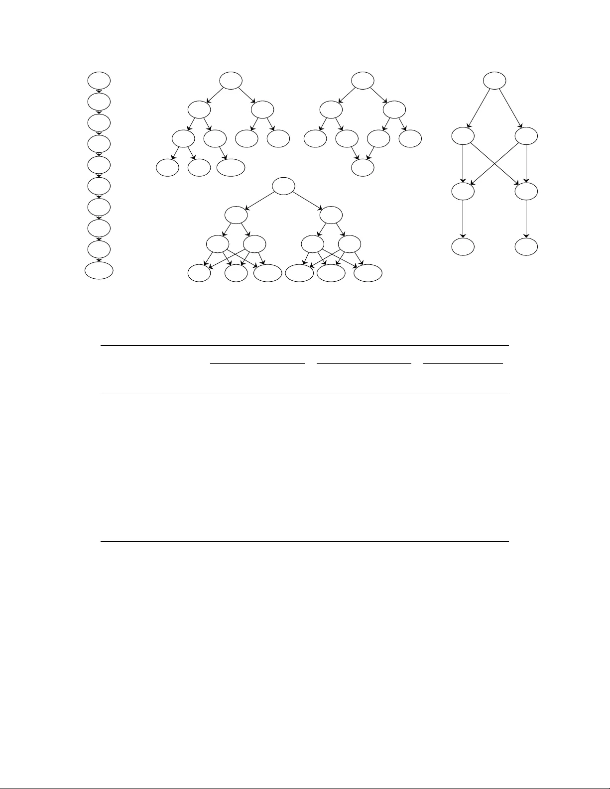
Discrete Causal Represen tation Learning W enjin Zhang ∗ Yixin W ang † Y uqi Gu ∗ ∗ Departmen t of Statistics, Colum bia Univ ersity † Departmen t of Statistics, Univ ersit y of Michigan Abstract Causal represen tation learning seeks to unco ver causal relationships among high- lev el laten t v ariables from lo w-level, en tangled, and noisy observ ations. Existing ap- proac hes often either rely on deep neural net w orks, whic h lack interpretabilit y and formal guarantees, or imp ose restrictive assumptions lik e linearity , con tin uous-only observ ations, and strong structural priors. These limitations particularly challenge applications with a large n um b er of discrete laten t v ariables and mixed-t yp e observ a- tions. T o address these challenges, w e prop ose discr ete c ausal r epr esentation le arning (DCRL) , a generativ e framew ork that mo dels a directed acyclic graph among discrete laten t v ariables, along with a sparse bipartite graph linking laten t and observ ed lay ers. This design accommo dates con tin uous, coun t, and binary resp onses through ﬂexible measuremen t mo dels while maintaining interpretabilit y . Under mild conditions, we pro v e that both the bipartite measuremen t graph and the latent causal graph are iden- tiﬁable from the observed data distribution alone. W e further prop ose a three-stage estimate-r esample-disc overy pip eline: p enalized estimation of the generativ e model pa- rameters, resampling of latent conﬁgurations from the ﬁtted mo del, and score-based causal disco v ery on the resampled latents. W e establish the consistency of this pro- cedure, ensuring reliable recov ery of the latent causal structure. Empirical studies on educational assessment and syn thetic image data demonstrate that DCRL recov ers sparse and interpretable laten t causal structures. Keyw ords: Causal Disco very; Causal Representation Learning; Directed Acyclic Graph; Iden tiﬁability; Discrete Laten t V ariables. 1 In tro duction Causal represen tation learning (CRL) seeks to recov er high-level laten t v ariables and their causal structure from low-lev el, entangled observ ations such as images, text, or time series Corresp ondence to: Y uqi Gu. Email: yuqi.gu@columbia.edu . Address: 928 SSW Building, 1255 Amsterdam Av enue, New Y ork, NY 10025. 1 ( Sc h¨ olk opf et al. , 2021 ; Moran and Aragam , 2026 ). While deep generative mo deling ap- proac hes to CRL hav e sho wn strong empirical p erformance on complex data ( Y ang et al. , 2021 ; Khemakhem et al. , 2020 ; Ja v aloy et al. , 2023 ; F an et al. , 2025 ), their neural architec- tures remain blac k b o xes with limited interpretabilit y , imp eding v alidation and understand- ing of what latent v ariables represent ( Moran and Aragam , 2026 ). In terpretability and identiﬁabilit y of mo dels are therefore central to uncov ering latent causal mechanisms in complex datasets in a trustw orthy manner. Informally , a causal rep- resen tation is identiﬁable if the observed distribution uniquely determines the parameters of the laten t v ariable mo del and the causal relations among these latents, up to a sp eciﬁed equiv alence relation capturing the unav oidable indeterminacies. Without identiﬁabilit y , rep- resen tation learning is prone to practical failures suc h as undersp eciﬁcation and p osterior collapse ( D’Amour et al. , 2022 ; W ang et al. , 2021 ). In this work, w e study causal structure learning in latent v ariable mo dels with discr ete latent v ariables and general-resp onse ob- serv ed v ariables. The mo del has t w o structural comp onen ts: a directed acyclic graph (DA G) among the latent v ariables and a sparse bipartite measurement graph linking the latents to the observ ables. Our goal is to determine when these structures are iden tiﬁable from the observ ational distribution alone, and to develop a consisten t pro cedure for reco vering them. A gro wing b ody of CRL work has established that, with c ontinuous latent v ariables, one can typically recov er latents only up to p erm utations and per-co ordinate reparameterizations ( v on K ¨ ugelgen et al. , 2023 ; Jin and Syrgk anis , 2024 ), rather than to a unique canonical form. Moreov er, such equiv alence classes are essen tially tight: without additional structure or side information, stronger iden tiﬁability is unattainable ( V arici et al. , 2025 ). Ev en in a fully linear mo del with p erfect single-no de interv entions, identiﬁabilit y is limited to scaling and p erm utation ( Squires et al. , 2022 ; Buchholz et al. , 2023 ). This inherent indeterminacy prev ents sp eciﬁc numerical v alues of laten t v ariables from carrying stable semantic meaning, ev en in identiﬁable contin uous-laten t CRL mo dels. 2 By con trast, discrete latent models with ev en highly nonlinear measuremen ts can achiev e iden tiﬁability up to latent-coordinate p erm utation alone ( Lee and Gu , 2024 , 2025 ). Con- sequen tly , while contin uous v ariables app ear more expressive, only a limited p ortion of the information they enco de is in v ariant under allow able reparameterizations and therefore ro- bustly in terpretable. Discrete latent v ariable mo dels th us oﬀer a more stable form of in- terpretabilit y: the equiv alence classes are smaller and easier to characterize, and latent co ordinates can b e more directly aligned with the ground truth causal factors. F rom a practical p ersp ectiv e, this discreteness is also often the right abstraction: in man y settings, the goal is to infer an unobserved state that drives observ ations and supports down- stream decisions, rather than to estimate a calibrated real-v alued quantit y . F or instance, in medicine, probabilistic mo dels often represen t diseases as discrete laten t v ariables that gen- erate observed symptoms or test results, so diﬀeren t latent-state conﬁgurations corresp ond to diﬀeren t clinical regimes ( Shw e et al. , 1991 ). In educational measurement, cognitive di- agnosis mo dels are p opular to ols that employ discrete latent v ariables to mo del a studen t’s mastery/deﬁciency of multiple latent skills( Rupp and T emplin , 2008 ; von Da vier and Lee , 2019 ). In suc h domains, learning a con tinuous laten t co ordinate ﬁrst and then imp osing cutoﬀs yields non-canonical thresholds whose meanings can shift under scaling without ad- ditional anc horing. Discrete laten t v ariables instead represent the abstractions directly . Motiv ated b y these considerations, we prop ose a discr ete c ausal r epr esentation le arn- ing (DCRL) framework in whic h (i) discrete latent v ariables follow a latent D A G, and (ii) observ ations are generated through a sparse measuremen t graph linking the laten t and ob- serv ed lay ers with ﬂexible mixed-type likelihoo ds. This framework accommo dates contin u- ous, coun t, and binary resp onses while allowing highly nonlinear latent-observ ation relation- ships. Within this new framework, our con tributions are threefold. First , despite the expressiv eness of the prop osed framework, we establish formal identiﬁ- abilit y guaran tees from a single observ ational distribution, without requiring in terv entions, 3 m ultiple environmen ts, or observed auxiliary v ariables. Our main con tribution is generic iden tiﬁability: under mild conditions, outside a measure-zero set of parameter v alues, the laten t distribution, measurement lay er, and latent DA G are iden tiﬁable from the observed data distribution, uniquely up to latent lab el p erm utations, so the una v oidable equiv alence class consists solely of relab elings of latent v ariables. Generic identiﬁabilit y is directly anal- ogous to how faithfulness excludes measure-zero violations of conditional indep endences in causal graphical mo dels ( Spirtes et al. , 2000 ; Ghassami et al. , 2020 ). Under additional design conditions, w e also obtain a stronger strict identiﬁabilit y statement. Se c ond , we prop ose and analyze a mo dular three-stage estimation pip eline. Stage I ﬁts the discrete generativ e pro cess b y p enalized maximum likelihoo d via a sto c hastic approx- imation exp ectation-maximization (SAEM) algorithm with sp ectral initialization, yielding estimates of the latent distribution and measuremen t graph while remaining computationally eﬃcien t. Stage I I resamples latent conﬁgurations from the ﬁtted laten t la w to construct a syn thetic dataset in the laten t space. Stage I I I applies Greedy Equiv alence Search (GES) ( Chic kering , 2002 ) to this resampled latent dataset to reco ver the laten t D AG. The v alidity of this algorithm relies on a k ey theoretical question: whether GES remains v alid when it op erates on samples from an estimate d latent law rather than from the true one. W e answ er this by extending classical notions of consistency and lo cal consistency for scoring criteria to a rate-robust setting that p ermits the scoring distribution to conv erge to the truth at a con trolled rate. Our analysis pro vides an explicit coupling b et w een the conv ergence rate in Stage I and the resampling size in Stage I I that guarantees GES applied to the resampled laten ts still recov ers the Marko v equiv alence class of the true latent DA G. Thir d , we show that DCRL can reveal meaningful laten t causal structure from data and yield in terpretable discrete causal factors in practice. Through tw o empirical studies in edu- cational assessmen t data and high-dimensional image data, w e ﬁnd that the learned latents align closely with domain-sp eciﬁc concepts and that the recov ered laten t DA G captures the 4 underlying causal dep endencies. Organization. Section 2 introduces the DCRL framework. In Section 3 , we establish iden- tiﬁabilit y results for DCRL. Section 4 describ es the prop osed three-stage estimation pip eline and establishes its theoretical consistency guaran tees. Section 5 and Section 6 presen t sim- ulation studies and real data applications, resp ectiv ely , to demonstrate the eﬀectiveness of our approach. Section 7 concludes the pap er with a discussion of p oten tial extensions. All pro ofs are deferred to the Supplemen tary Material. Notation. W e write a N = ω ( b N ) (resp. a N = o ( b N )) if a N b N → ∞ (resp. a N b N → 0) as N → ∞ . F or a p ositiv e in teger n , we write [ n ] = { 1 , . . . , n } . F or any vector u ∈ R K , deﬁne supp( u ) := { k ∈ [ K ] : u k  = 0 } . F or a matrix A , we use A i, : (resp. A : ,j ) for its i -th row (resp. j -th column). F or vectors x, y ∈ R d , write x ⪰ y (resp. x ⪯ y ) if x k ≥ y k (resp. x k ≤ y k ) for all k = 1 , . . . , d . W e write G ⋊ H for the semidirect pro duct of groups G and H . F or a set A in a top ological space, we write A ◦ for the interior of A . 2 Discrete Causal Represen tation Learning F ramew ork Causal Graphical Mo dels. W e b egin by reviewing essen tial deﬁnitions to ﬁx notation. Let R = ( R 1 , . . . , R d ) be random v ariables with joint distrib ution p ⋆ ( R ). W e consider graphs G = ( V , E ), where V = 1 , . . . , d corresp onds to the v ariables R i and E ⊆ V × V is the set of edges. A directed acyclic graph (DA G) is a directed graph with no cycles. W e now relate these graphs to conditional indep endencies. F or a distribution p on R = ( R 1 , . . . , R d ), let I ( p ) := { ( A ⊥ ⊥ B | C ) p : R A ⊥ ⊥ p R B | R C } denote the set of all conditional indep endence statements that hold under p , where A, B , C ⊆ V are pairwise disjoint and R A = { R i : i ∈ A } . Let I ( G ) := { ( A ⊥ ⊥ B | C ) G : R A ⊥ ⊥ G R B | R C } b e the collection of conditional indep endences enco ded b y a DA G G via d-separation. W e sa y p is Mark ov with resp ect to G if I ( G ) ⊆ I ( p ). W rite M ( G ) := { p : I ( G ) ⊆ I ( p ) } . F or D A Gs, p ∈ M ( G ) is equiv alent to the factorization of the join t density according to G : p ( R ) = Q d i =1 p ( R i | R P a G i ), 5 where Pa G i is the parent set of no de i in G ( Lauritzen , 1996 ). W e call p faithful to G if I ( p ) ⊆ I ( G ) ( Koller and F riedman , 2009 ). Combining the tw o inclusions, a distribution is DA G-p erfect ( Chick ering , 2002 ) to G if I ( G ) = I ( p ), so that G enco des exactly all conditional indep endences of p . In this case, G is a p erfect map of p . W e say G 1 and G 2 are Mark ov equiv alen t if I ( G 1 ) = I ( G 2 ), and write G 1 ≡ G 2 . Mark ov- equiv alent DA Gs form a Marko v equiv alence class. Tw o DA Gs are Marko v equiv alen t if and only if they ha v e the same sk eleton and v-structures ( V erma and P earl , 1990 ). Eac h Marko v equiv alence class can be uniquely represen ted b y a completed partially directed acyclic graph (CPD AG), in whic h an edge i → k is directed if and only if it has the same orien tation in ev ery DA G in the class, and an edge i − k is undirected if b oth orien tations i → k and i ← k o ccur among the DA Gs in the class ( V erma and Pearl , 1990 ; Chick ering , 2002 ). A c ausal gr aphic al mo del consists of a DA G G and a distribution p that is Marko v to G , with directed edges interpreted causally . In this pap er we are primarily in terested in discr ete c ausal gr aphic al mo dels , where each v ariable R i tak es v alues in a ﬁnite state space and ( G, p ) is a causal graphical mo del. Discrete Causal Represen tation Learning. W e tak e the causal structure as primitive and place probabilistic distributions on top of it. W e work with a collection of v ariables con- sisting of b oth observ able and latent comp onen ts. Let X = ( X 1 , . . . , X J ) ∈ × J j =1 X j denote the observ ed v ariables, where X j ⊆ R is allo wed to be general. In particular, our form ulation accommo dates a wide range of data t yp es, including con tinuous measurements, coun t-v alued observ ations, and binary or categorical resp onses. W e consider binary latent v ariables and denote them by Z = ( Z 1 , . . . , Z K ) ∈ { 0 , 1 } K , where K ≥ 2. The causal structure is sp eci- ﬁed b y (i) a directed acyclic graph (DA G) G on the latent v ariables Z 1 , . . . , Z K , and (ii) a directed bipartite structure Q = ( q j,k ) ∈ { 0 , 1 } J × K from the laten t v ariables to the observed v ariables, where q j,k = 1 if and only if Z k is a direct cause of X j for j ∈ [ J ] and k ∈ [ K ]. The bipartite graph describ es the measurement mo deling structure. T ogether, ( G , Q ) determines 6 a full acyclic causal graph on ( Z , X ). An illustration is provided in Figure 1 . Z 1 Z 2 · · · · · · Z K X 1 X 2 · · · · · · · · · · · · · · · · · · · · · · · · X J · · · · · · · · · · · · Q : causal relations between X and Z G : causal relations among Z Figure 1: Laten t D A G and measuremen t graph in discrete causal representation learning T o obtain a data-generating pro cess from ( G , Q ), we view the join t distribution of the laten t v ariables as the primitiv e ob ject and assume that it satisﬁes the Marko v factorization asso ciated with G . Let p = ( P ( Z = z )) z ∈{ 0 , 1 } K denote the 2 K -dimensional probability vector of Z with p ∈ M ( G ). Equiv alen tly , p factorizes according to G as p ( Z ) = Q K k =1 p ( Z k | Z P a G k ), whic h enco des the directed dep endencies prescrib ed b y the laten t D A G G . Next, w e sp ecify how the latent causes act on the observed v ariables according to Q . F or each item j ∈ [ J ], let K j = { k ∈ [ K ] : q j,k = 1 } b e the index set of its laten t parents. W e write the linear predictor η j ( z ) as a multilinear p olynomial in the binary laten t vector z = ( z 1 , . . . , z K ) ∈ { 0 , 1 } K . F or any subset S ⊆ [ K ], deﬁne the monomial feature ϕ S ( z ) := Q k ∈ S z k , with the conv ention ϕ ∅ ( z ) ≡ 1. Fix once and for all an ordering ( S 1 , . . . , S 2 K ) of all subsets of [ K ]. Let ϕ ( z ) ∈ { 0 , 1 } 2 K b e the corresp onding feature v ector with entries ϕ m ( z ) = ϕ S m ( z ). F or item j , collect coeﬃcients in to β j ∈ R 2 K b y ( β j ) m := β j,S m , and imp ose ( β j ) m = 0 whenever S m ⊈ K j , so that only main eﬀects and in teractions among co ordinates in K j are allow ed. Equiv alen tly , η j ( z ) = β ⊤ j ϕ ( z ) = P S ⊆ K j β j,S Q k ∈ S z k . Stacking the ro ws yields the matrix B = [ β 1 . . . β J ] ⊤ ∈ R J × 2 K . In practice, it is often suﬃcient to restrict atten tion to the main eﬀects of the latent causes, which corresp onds to setting β j,S = 0 whenev er | S | > 1. In this case, the linear predictor reduces to η j ( z ) = β j, ∅ + P k ∈ K j β j,k z k , whic h is analogous to a generalized linear 7 sp eciﬁcation with an in tercept and main eﬀects in the binary latent vector z as co v ariates. Compared with the all-eﬀect sp eciﬁcation, this restriction reduces the num b er of parameters from 2 K to | K j | + 1 p er item, yielding a more parsimonious and interpretable sp eciﬁcation. In our subsequen t estimation pro cedure, w e will primarily focus on this main-eﬀect speciﬁcation. Conditionally on Z , we mo del each X j b y an item-sp eciﬁc parametric family consistent with Q and assume conditional indep endence across j giv en Z : X j | Z ∼ ParF am j  g j  η j ( Z ) , γ j   , j ∈ [ J ] . (1) Here P arF am j = { P j, θ : θ ∈ H j } is a known family with parameter space H j ⊆ R h j , and g j : R × [0 , ∞ ) → H j is a known link mapping the linear predictor η j ( · ) and, when applicable, a disp ersion parameter γ j > 0 to the parameter of P arF am j . W rite γ = ( γ 1 , . . . , γ J ). In tegrating out the latent Z yields the marginal law of the observ ables, P ( X ) = X z ∈{ 0 , 1 } K P  X | Z = z  P ( Z = z ) , (2) whic h is determined by the triple ( p , B , γ ) together with the causal structure ( G , Q ). Deﬁnition 1. We c onsider the fol lowing discr ete c ausal r epr esentation le arning data-generating pro cess p ar ameterize d by ( p , G , B , Q , γ ) , wher e the mar ginal law of the observe d data is given by ( 2 ) . When G and Q ar e known and ﬁxe d, this induc es a family of pr ob ability distributions on X , indexe d by ( Θ , G , Q ) , which we denote by P Θ , G , Q , wher e Θ := ( p , B , γ ) . Remark 1. F or clarity, Se ction 2 pr esents the fr amework under binary latent attributes Z k ∈ { 0 , 1 } . A l l c omp onents extend to or der e d p olytomous attributes Z k ∈ [ M k ] = { 0 , 1 , . . . , M k − 1 } . In the extension, η j is stil l a line ar c ombination of c o eﬃcients { β j, u } indexe d by latent “states” u , and a term β j, u c ontributes to η j ( z ) only when u ⪯ z c o or dinatewise. Mor e over, β j, u is nonzer o only if supp( u ) ⊆ K j . The extension and its generic identiﬁability r esult ar e state d in Se ction 3 , with ful l deﬁnitions in App endix S.4 . 8 T aken together, the DCRL framew ork yields a highly ﬂexible and p oten tially strongly nonlinear measuremen t la y er from the laten t conﬁguration to the observed resp onses. On the one hand, the all-eﬀect speciﬁcation for η j ( z ) allo ws arbitrary interaction patterns among the laten t v ariables, including highest–order interactions o ver all attributes in K j . On the other hand, by allowing a general parametric family P arF am j and link mapping g j , we imp ose no single ﬁxed resp onse family , so that a wide range of nonlinear conditional distributions X j | Z can b e accommo dated. Under DCRL, the complete causal structure comprises tw o comp onen ts: the DA G G among latent v ariables Z 1 , . . . , Z K , and the directed bipartite structure Q from laten t v ari- ables to observed v ariables. Our goal is to join tly reco v er G and Q from X . Connections with Existing Studies. Most identiﬁable mo dels for causal discov ery with partially unobserv ed v ariables rely on linearity ( Anandkumar et al. , 2013 ; Squires et al. , 2022 ; Huang et al. , 2022 ; Dong et al. , 2026 ), an assumption that often fails in practice. Bey ond linearit y , iden tiﬁabilit y has also b een established for certain nonlinear latent hierarchical mo dels ( Prashant et al. , 2025 ). How ev er, those results imp ose m uch stronger restrictions on the laten t causal architecture than ours. See Supplemen t S.9 for more details. 3 Iden tiﬁabilit y Before introducing our identiﬁabilit y notion, w e ﬁrst relate our framew ork to the statistical- iden tiﬁability form ulation used in recent CRL work ( Xi and Blo em-Reddy , 2023 ; Moran and Aragam , 2026 ). Consider the mo del X = f ( Z ) + ϵ , where Z ∈ Z is the latent v ariable, f : Z → X is the representation map, and ϵ is noise. Let F b e a class of admissible maps f , and let P b e a class of admissible laten t distributions p on Z . F or any bijection ξ : Z → Z , one may rewrite the mo del as X = ( f ◦ ξ − 1 )( ξ ( Z )) + ϵ . Therefore, without restrictions on F and P , the mo del is trivially noniden tiﬁable. T o formalize this, let ξ # p denote the push- forw ard of p b y ξ . One calls ξ an indeterminacy transformation if f ◦ ξ − 1 ∈ F and ξ # p ∈ P . The collection of all suc h transformations is the indeterminacy set A ( F , P ). Equiv alen tly , 9 A ( F , P ) indexes the “transformation-based” comparison class { ( f ◦ ξ − 1 , ξ # p ) : ξ ∈ A ( F , P ) } asso ciated with a ﬁxed pair ( f , p ). The key question is to determine which restrictions on F and P mak e A ( F , P ) small while remaining ﬂexible. Our DCRL framework ﬁts naturally into this framew ork. Here Z = { 0 , 1 } K . F or Gaus- sian resp onses and iden tity link, we ma y write X j = η j ( Z ) + ε j with ε j ∼ N (0 , γ 2 j ), so that f ( Z ) = ( η 1 ( Z ) , . . . , η J ( Z )) ∈ R J . F or a ﬁxed latent DA G G and measurement graph Q , the corresp onding classes can b e viewed as P G := { p on { 0 , 1 } K : p is Mark o v to G } , and F Q := { f = ( η 1 , . . . , η J ) : { 0 , 1 } K → R J : η j ( z ) = η j ( z ′ ) whenev er z K j = z ′ K j , ∀ j } . Addi- tional assumptions used later in the paper can b e understoo d precisely as further restrictions on P G and F Q , imp osed to shrink the admissible indeterminacy set. This viewp oin t is conceptually useful, but it is imp ortan t to distinguish settings where the full statistical equiv alence class coincides with the transformation-based class indexed b y A ( F , P ) from those where it do es not. In identiﬁable CRL, it is widely assumed that the generativ e map f is injective ( Ahuja et al. , 2023 ; Hartford et al. , 2023 ) and that the obser- v ation mo del is well-posed in the sense that the distribution of f ( Z ) is determined by that of X = g ( f ( Z ) , ϵ ). A simple suﬃcien t condition is an additive and indep enden t observ ation- noise mo del X = f ( Z ) + ϵ with Gaussian noise distribution. Under these commonly used injectiv e-generator and well-posed observ ation assumptions, Xi and Blo em-Reddy ( 2023 , Lemma 2.1) shows that if tw o parameterizations ( f a , p a ) and ( f b , p b ) induce the same obser- v ational distribution, then they must b e related b y a latent-space automorphism ξ ∈ Aut( Z ) in the sense that f b = f a ◦ ξ − 1 and p b = ξ # p a up to null sets. Hence, for suc h mo dels, re- stricting atten tion to the transformation-based comparison class (equiv alently , studying the indeterminacy set A ( F , P )) en tails no loss of generality . In the discrete case Z = { 0 , 1 } K , suc h a ξ is simply a p erm utation of the ﬁnite latent state space, so ξ # p is merely a relab eling of p and the remaining transformation-based comparison is ﬁnite. In contrast, our DCRL framew ork do es not directly assume a well-posed observ ation 10 mo del in the ab o v e sense. Without this end-to-end w ell-p osedness assumption, which would b ypass muc h of the substan tive diﬃculty , the reduction from general parameter-level equiv- alence to the transformation-based comparison class indexed by A ( F , P ) is no longer auto- matic. Accordingly , w e b egin by comparing arbitrary admissible parameter triples (Θ , G , Q ) and ( e Θ , e G , e Q ) that induce the same observ ational distribution, and then enforce this reduc- tion b y imp osing explicit, v eriﬁable structural restrictions enco ded b y Q , together with more delicate techniques tailored to our mo del class. This additional collapse step is precisely what mak es our analysis more inv olved than approac hes that assume well-posedness directly . Before pro ceeding, w e ﬁrst sp ecify the parameter spaces. Deﬁne Ω K ( Θ ; G , Q ) := n Θ : G is a p erfect map of p , β j,S = 0 if S ⊈ K j , β j, { k }  = 0 iﬀ k ∈ K j o . Ω K ( Θ , G , Q ) := n ( Θ , G , Q ) : Θ ∈ Ω K ( Θ ; G , Q ) o . No w w e in tro duce the equiv alence relation that sp eciﬁes the unav oidable am biguit y , and then deﬁne generic identiﬁabilit y relative to this equiv alence. Deﬁnition 2. F or the discr ete CRL fr amework, deﬁne an e quivalenc e r elationship “ ∼ K ” by setting ( Θ , G , Q ) ∼ K ( ˜ Θ , ˜ G , ˜ Q ) iﬀ γ = ˜ γ and ther e exists a p ermutation σ ∈ S [ K ] such that the fol lowing hold. First, p ( z σ (1) ,...,z σ ( K ) ) = ˜ p z for al l z ∈ { 0 , 1 } K and G ≡ σ ( ˜ G ) , wher e σ ( ˜ G ) denotes the DA G obtaine d fr om ˜ G by r elab eling e ach no de k as σ ( k ) . Se c ond, q j,k = ˜ q j,σ ( k ) for al l j ∈ [ J ] , k ∈ [ K ] , and for al l j and S ⊆ [ K ] , β j,S = ˜ β j,σ ( S ) , wher e σ ( S ) := { σ ( k ) : k ∈ S } . Deﬁnition 3. L et ( Θ ⋆ , G ⋆ , Q ⋆ ) ∈ Ω K ( Θ , G , Q ) b e the true p ar ameter triple of the discr ete c ausal r epr esentation le arning fr amework. The fr amework is generic al ly identiﬁable up to ∼ K if { Θ ∈ Ω K ( Θ ; G ⋆ , Q ⋆ ) : ∃ ( e Θ , e Q , e G ) ∼ K ( Θ , Q ⋆ , G ⋆ ) such that P e Θ , e Q , e G = P Θ , Q ⋆ , G ⋆ } is a me asur e-zer o set with r esp e ct to Ω K ( Θ ; G ⋆ , Q ⋆ ) . This equiv alence relation ∼ K is the discrete analogue of the transformation-based inde- terminacies enco ded b y A ( F , P ), sp ecialized to latent-coordinate relab elings. 11 The measure-zero qualiﬁer in Deﬁnition 3 parallels the faithfulness conv ention in causal disco very: for a ﬁxed DA G, distributions that are Mark o v but unfaithful form a Leb esgue- n ull subset of the parameter space, so faithfulness excludes only a negligible set of degenerate conﬁgurations. Our generic-iden tiﬁability deﬁnition plays the same role here. After imposing the latent Mark o v-plus-faithfulness condition on p , non-identiﬁabilit y can still o ccur for exceptional v alues of the contin uous measurement parameters ( B , γ ), but these exceptional conﬁgurations form a Lebesgue-null set. Hence, restricting atten tion to generic iden tiﬁabilit y excludes only a measure-zero subset of “bad” ( B , γ ) conﬁgurations. In this sense, the loss incurred b y discarding measure-zero subsets of parameters is as harmless as the loss incurred when imp osing faithfulness in the ﬁrst place. One may also consider the stronger notion of strict iden tiﬁability , under which equality of observ ational distributions implies equiv alence up to ∼ K for every admissible parameter triple, rather than for all but a measure-zero subset. W e do not emphasize this stronger notion in the main text, b ecause the corresp onding strict-iden tiﬁability statements together with several related extensions can b e obtained by adapting existing arguments from Liu et al. ( 2025 ); Lee and Gu ( 2025 ). W e therefore record these formal results in Section S.1 . W e no w in tro duce the assumptions needed for our generic iden tiﬁabilit y result. Assumption 1. (a) G is a p erfe ct map of p and p z ∈ (0 , 1) for al l z ∈ { 0 , 1 } K . (b) F or e ach item j , η j ( z ) > η j ( z ′ ) whenever z ⪰ Q j, : and z ′ ⪰ Q j, : . Assumption 1 (a) is a restriction on the latent distribution class P G . Assumption 1 (b) is a restriction on F Q : it imp oses a monotonicity condition on each item resp onse function η j . This type of condition is also used in Liu et al. ( 2025 ); Lee and Gu ( 2025 ) to av oid the sign-ﬂipping for each latent v ariable. T o ensure generic identiﬁabilit y , w e in tro duce an additional analytic assumption, which holds for regular minimal exp onen tial families on the interior of natural parameter spaces. 12 Assumption 2. F or e ach j ∈ [ J ] , deﬁne the c anonic al c ountable sep ar ating class C can j := {X j ∩ ( a, b ] : a, b ∈ Q , a < b } ∪ {X j } . Assume that H ◦ j  = ∅ , and that the fol lowing hold. (i) F or every S ∈ C can j , the map θ 7→ P j, θ ( S ) is r e al-analytic on H ◦ j . (ii) P j, θ = P j, θ ′ implies θ = θ ′ for al l θ , θ ′ ∈ H ◦ j . (iii) The link g j maps R × (0 , ∞ ) into H ◦ j and is r e al-analytic. Mor e over, exactly one of the fol lowing holds. (a) (No disp ersion) The link is indep endent of γ and the slic e map η 7→ g j ( η , γ 0 ) is inje ctive for some (e quivalently, any) ﬁxe d γ 0 ∈ [0 , ∞ ) . (b) (With disp ersion) The ful l map ( η , γ ) 7→ g j ( η , γ ) is inje ctive on R × (0 , ∞ ) . Our main identiﬁabilit y result is stated in the following theorem. Theorem 1. Under Assumptions 1 and 2 , DCRL is generic al ly identiﬁable if the fol lowing hold. (i) After a r ow p ermutation, we c an write Q ⋆ = [ Q ⊤ 1 , Q ⊤ 2 , Q ⊤ 3 ] ⊤ , wher e Q 1 , Q 2 ∈ { 0 , 1 } K × K have unit diagonals (oﬀ–diagonals arbitr ary), and Q 3 has no al l-zer o c olumn. (ii) No c olumn of Q ⋆ c ontains another: for any p  = q , neither Q ⋆ : ,p ⪰ Q ⋆ : ,q nor Q ⋆ : ,q ⪰ Q ⋆ : ,p . Condition (i) is b est viewed as a weak cov erage requirement on the measuremen t design: it guarantees that ev ery laten t co ordinate aﬀects at least one observed v ariable, and that there exist some anchor-lik e items in which each latent is forced to app ear. Ho wev er, it is w eak in the sense that suc h anchor-lik e items may still dep end on many other latents. Our condition (ii) coincides with Condition 3.1 (the subset condition) in Kivv a et al. ( 2021 ). As they observed, violating this subset condition can lead to non-identiﬁabilit y . Similarly , we emphasize that condition (i) alone is not suﬃcien t for generic iden tiﬁabilit y . In particular, App endix S.2 constructs a model satisfying condition (i) in whic h Q has distinct columns and eac h column con tains at least one zero, yet the framew ork fails to b e generically identiﬁable. 13 Our pro of is a three-step reduction of the comparison class. First, a Krusk al-type tensor argumen t collapses the original con tinuous parameter comparison to a ﬁnite, transformation- generated comparison class: any remaining competitor with the same observ ational la w m ust b e of the form ( ξ # p , η ◦ ξ − 1 ), where ξ ∈ S 2 K is a p erm utation of the 2 K laten t states of Z . Th us, after the tensor step, w e are essen tially in the setting of Moran and Aragam ( 2026 ), and the problem b ecomes how to shrink the indeterminacy set A ( F , P ) = S 2 K . Before further reducing A ( F , P ), we ﬁrst iden tify Q : using Assumption 1 (b) and an inclusion–exclusion argumen t on the transformed η -arra y , w e sho w that all these 2 K admissible comp etitors m ust ha ve measurement matrices that agr ee with the true Q up to a co ordinate p erm utation. This observ ation makes the structural constrain t on F Q m uch clearer. W e then return to reducing A ( F , P ): the subset condition, together with the structural constrain t on F Q , reduces the indeterminacy set from S 2 K to ( Z 2 ) K ⋊ S K , corresp onding to co ordinate p erm utations com- bined with co ordinatewise bit-ﬂips, and Assumption 1 (b) further rules out bit-ﬂips, lea ving only co ordinate relab elings in S K . Finally , β and G are reco v ered from the in v ertible linear map η ↔ β and the p erfect-map condition, yielding identiﬁabilit y . Extension to P olytomous A ttributes. The binary-laten t framew ork of Section 2 extends naturally to the case where eac h laten t attribute Z k tak es v alues in [ M k ] = { 0 , 1 , . . . , M k − 1 } with M k ≥ 2. The linear predictor η j ( z ) generalizes to a sum o v er co eﬃcien ts { β j, u } indexed b y u ∈ Q K k =1 [ M k ], where β j, u con tributes to η j ( z ) only if supp( u ) ⊆ K j and u ⪯ z co ordinatewise, thereby preserving b oth the sparsity structure enco ded by Q and the causal in terpretation of eac h en try q j,k . Under Assumption 1 (a), Assumption 2 , and an ordered-lev el analogue of the monotonicit y condition in Assumption 1 (b) (Assumption S.3 ), we establish generic identiﬁabilit y (Theorem S.2 in Section S.4 ) with t wo k ey diﬀerences from the binary case. First, the measuremen t design requires at least 2 P K k =1 ⌈ log 2 M k ⌉ + 1 observed v ariables, whic h grows only logarithmically in the n um b ers of categories and is order-sharp for the general-resp onse setting. Second, b ecause the inclusion–exclusion reconstruction of Q do es 14 not directly extend to the polytomous setting, w e instead use the subset condition to identify Q and shrink the indeterminacy set; this corresp onds to within-co ordinate lev el p erm utations comp osed with across-co ordinate relab elings. W e then use the monotonicity condition to eliminate the within-co ordinate p erm utations, leaving only co ordinate relab elings. Unlike in the binary case, this group-reduction step excludes a Lebesgue-null exceptional set, reﬂ ecting the gen uine additional diﬃculty of the p olytomous setting; see Supplement S.4 for details. Nonparametric Disentanglemen t. As a further consequence, we obtain a nonparametric disen tanglement result in the following corollary . Corollary 1. L et Z = Q K k =1 [ M k ] , wher e M k ≥ 2 , and c onsider the r epr esentation mo del X = f ( Z ) + ϵ , wher e f = ( f 1 , . . . , f J ) : Z → R J . F or a binary matrix Q = ( q j,k ) ∈ { 0 , 1 } J × K , write K j := { k ∈ [ K ] : q j,k = 1 } . Deﬁne P := { p on Z : P z ∈Z p z = 1 } and F := ( f : Z → R J      ∃ Q ∈ { 0 , 1 } J × K s.t., neither Q : ,a ⪰ Q : ,b nor Q : ,b ⪰ Q : ,a , ( ∀ a  = b ) , f j ( z ) = f j ( z ′ ) whenever z K j = z ′ K j ( j ∈ [ J ]) , f j ( z )  = f j ( z ′ ) whenever z K j  = z ′ K j ( j ∈ [ J ]) ) Then every admissible indeterminacy tr ansformation ξ ∈ A ( F , P ) c an only p ermute c o or di- nates (with the same numb er of c ate gories) and r elab el the levels within e ach c o or dinate. Corollary 1 establishes disen tanglemen t in the sense of Moran and Aragam ( 2026 ): among all admissible latent bijections ξ : Z → Z that preserve mem b ership in ( F , P ), the only ones that remain are element-wise transformations and p erm utations. Notably , this con- clusion is obtained with f treated nonparametrically , sub ject only to the restrictions in F , rather than under a sp eciﬁc parameterization like all-eﬀect forms. Moreo ver, under injectiv e-generator and w ell-p osed observ ation assumptions that are common in identiﬁable CRL ( Ahuja et al. , 2023 ; Khemakhem et al. , 2020 ), the full statistical equiv alence class co- incides with the transformation-based indeterminacy class ( Xi and Blo em-Reddy , 2023 ), so 15 the corollary yields a direct disen tanglemen t conclusion from observ ational data alone. This con trasts with m uch of the existing literature, where even after adopting the same base- line, additional sources of v ariation—suc h as auxiliary v ariables, multiple environmen ts, or in terven tions—are t ypically inv oked to further shrink the indeterminacy set do wn to p erm u- tations and comp onen t-wise transformations ( Khemakhem et al. , 2020 ; Ahuja et al. , 2023 ). In our framework, the structural constraints on f enco ded by Q together with the subset condition are already suﬃcien t to enforce this shrink age at the level of A ( F , P ) from obser- v ational data alone. This can b e viewed as a natural restriction when Q is used to describ e whic h latents aﬀect which measurements. Compared with other observ ational-only iden- tiﬁabilit y results, our assumptions are often milder: prior work commonly relies on anchor features ( Moran et al. , 2022 ; Prashan t et al. , 2025 ), Gaussian-mixture laten t structure ( Kivv a et al. , 2022 ), or access to a mixture oracle ( Kivv a et al. , 2021 ), whose existence can fail for common discrete-resp onse observ ation mo dels (see Supplement S.9 ). If one further imp oses a monotonicit y condition, the within-co ordinate relab elings here can also b e remo ved. 4 Estimation Pro cedure and Theoretical Guaran tees With a sligh t abuse of notation, w e let X denote the N × J data matrix with ro ws X 1 , . . . , X N . Similarly , let Z denote the corresponding N × K latent v ariable matrix with ro ws Z 1 , . . . , Z N . Giv en the b ottom-lay er data X ∈ R N × J with unknown laten t causal structures and param- eters ( p , G , B , Q , γ ), our ob jectiv e is to recov er Q and G . In this section, we pro vide the complete pip eline for recov ering the measurement graph and laten t D A G (Algorithm 1 ). Next, we describ e the pip eline in detail. In Stage I, we apply a p enalized maximum like- liho od estimator to obtain ( b p , b B , b γ ) and hence b Q , as detailed in Section 4.1 . In Stage I I, w e ﬁx a strictly increasing sampling rule f : Z + → Z + and draw f ( N ) i.i.d. latent samples from b p = ( b p z ) z ∈{ 0 , 1 } K to form the resampled matrix b Z ∈ { 0 , 1 } f ( N ) × K . The requiremen t that f b e strictly increasing is imp osed purely for notational conv enience, and our analysis dep ends only on the growth rate of f ( N ) relative to N . In Stage I II, w e run Greedy Equiv alence 16 Algorithm 1: Discrete Causal Representation Learning: Estimate-Resample-Discov ery Data: X , K , strictly increasing sampling rule f : Z + → Z + . Stage I: Parameter Estimation ; Obtain the estimated ( b p , b B , b γ ); Set b Q by the supp ort of b B : b q j,k ← 1 ( b β j,k  = 0); Stage I I: Laten t Resampling from b p ; Dra w f ( N ) i.i.d. samples Z (1) , . . . , Z ( f ( N )) i.i.d. ∼ b p and stack them into b Z ∈ { 0 , 1 } f ( N ) × K ; Stage I I I: Causal Disco very on Laten t Space ; P erform a causal disco very metho d on b Z to obtain the estimated b G ; Output: ( b p , b B , b γ , b Q , b G ). Searc h (GES; Chic k ering , 2002 ) on b Z to obtain an estimate b G ; details on GES are given in Section 4.2 . In Section 4.3 , we sp ecify suitable ranges for the resampling size f ( N ) and conditions to ensure that this three-stage pip eline enjoys rigorous consistency guaran tees. While our iden tiﬁability results hold for the all-eﬀect sp eciﬁcation, in practice we fo cus on the main-eﬀect sp eciﬁcation for parsimony , interpretabilit y , and computational tractability . 4.1 P enalized likelihoo d estimation via Gibbs–SAEM Let ℓ ( Θ | X ) = P N i =1 log P ( X i | Θ ) b e the marginal log-likelihoo d from ( 2 ), and deﬁne b Θ ∈ arg max Θ n ℓ ( Θ | X ) − p λ N ,τ N ( B ) o , (3) where p λ N ,τ N is an entrywise p enalt y extended additiv ely ov er B = ( β j,k ): p λ N ,τ N ( B ) = P K k =1 P J j =1 p λ N ,τ N ( β j,k ) . The bipartite matrix is then estimated by thresholding: b q j,k = 1 ( b β j,k  = 0) , j ∈ [ J ] , k ∈ [ K ] . (4) Throughout, we assume that the p enalt y p λ N ,τ N satisﬁes the regularity conditions in Lee and Gu ( 2025 , Supplemen t S.1.4), including standard truncated sparsity–inducing p enalties suc h as the truncated Lasso p enalt y (TLP) ( Shen et al. , 2012 ) and the smo othly clipp ed absolute deviation (SCAD) p enalt y ( F an and Li , 2001 ), and w e do not repro duce them here The follo wing result establishes consistency of the parameters and the bipartite graph. 17 Theorem 2 (Theorem 3 in Lee and Gu ( 2025 )) . L et ( Θ ⋆ , Q ⋆ , G ⋆ ) denote the true p ar ameters in the discr ete CRL fr amework. Supp ose the p ar ameter sp ac e is c omp act and al l entries of B ar e b ounde d, the data-gener ating pr o c ess at Θ ⋆ is identiﬁable and has nonsingular Fisher information, and the tuning p ar ameters satisfy 1 / √ N ≪ τ N ≪ λ N / √ N ≪ 1 . If b Θ solves ( 3 ) , then ther e exists a r elab eling ˜ Θ ∼ K b Θ such that ∥ ˜ Θ − Θ ⋆ ∥ = O p (1 / √ N ) . Mor e over, with ˜ Q c ompute d fr om ˜ Θ via ( 4 ) , one has P ( ˜ Q  = Q ⋆ ) → 0 . W e compute ( 3 ) via a p enalized Gibbs–SAEM algorithm ( Dely on et al. , 1999 ; Kuhn and La vielle , 2004 ; Lee and Gu , 2025 ). A direct EM implementation would require ev aluating the conditional exp ectation of the complete-data log-likelihoo d by summing ov er all 2 K laten t conﬁgurations. This leads to an O ( N J 2 K ) cost p er outer iteration, which b ecomes prohibitiv e once K is mo derate. Gibbs–SAEM sidesteps this by replacing the exact E–step with lo w-cost Gibbs up dates. The full pseudo co de is giv en in Algorithm S.2 in Section S.8.3 . In the E–step w e run an alternating co ordinate Gibbs sampler ( Gu and Xu , 2023 ) tar- geting the p osterior P ( Z | X ; Θ [ t ] ) under the parameter iterate Θ [ t ] = ( β [ t ] , γ [ t ] , p [ t ] ). In our implemen tation w e tak e a single Gibbs sweep p er outer iteration ( C = 1) follo wing Delyon et al. ( 1999 ). Within this sweep we visit each co ordinate Z i,k in turn. Conditional on the curren t v alue of all other co ordinates Z i, − k , the conditional distribution of Z i,k is Bernoulli with success probability P  Z i,k = 1 | Z i, − k , Y ; Θ [ t ]  ∝ P  Z i,k = 1 , Z i, − k ; p [ t ]  Q J j =1 P  X ij | Z i ; β [ t ] j , γ [ t ] j  , and similarly for Z i,k = 0. Equiv alently , the log-o dds of Z i,k = 1 versus 0 is giv en by the diﬀerence in log join t densities when ﬂipping that bit. This conditional has a closed form and is straightforw ard to sample from. T o keep each ﬂip inexp ensiv e, we main tain for every sample–item pair the linear score ψ ij = β [ t ] j, 0 + P K k =1 β [ t ] j,k Z ik , so that the lik eliho o d contribution of Z i to X ij can b e up dated by rank-one changes in ψ ij . Flipping a single bit Z i,k mo diﬁes all ψ ij b y adding or subtracting β [ t ] j,k , which costs O ( J ) op erations. A full Gibbs sw eep visits all K co ordinates for each of the N individuals, so the E–step costs O ( N J K ) p er outer iteration, in contrast to the O ( N J 2 K ) cost of exact EM when K grows. 18 The Gibbs sweep pro duces an up dated Z [ t +1] , inducing an empirical distribution on { 0 , 1 } K that we use to up date p via Robbins–Monro sto chastic approximation. W riting b p [ t +1] for the empirical prop ortions of the sampled conﬁgurations at iteration t + 1, w e set p [ t +1] = (1 − θ t +1 ) p [ t ] + θ t +1 b p [ t +1] , with stepsizes { θ t } t ≥ 1 satisfying P t θ t = ∞ and P t θ 2 t < ∞ . In the M–step, for eac h ro w j of B we set F [ t +1] j ( β j , γ j ) = (1 − θ t +1 ) F [ t ] j ( β j , γ j ) + θ t +1 C C X r =1 N X i =1 log P  X ij | Z i = Z [ t +1] ,r i ; β j , γ j  , where F [0] j ≡ 0 for j ∈ [ J ], and then solve the p enalized maximization ( β [ t +1] j , γ [ t +1] j ) = arg max β j ,γ j n F [ t +1] j ( β j , γ j ) − p λ N ,τ N ( β j ) o . T ogether, the Gibbs E–step and p enalized SAEM M–step pro vide an eﬃcient sto c hastic optimization scheme for the p enalized ob jective ( 3 ). In complex laten t v ariable mo dels, the p enalized SAEM algorithm ma y conv erge to lo cal maxima if p oorly initialized. T o mitigate this, w e adopt a sp ectral initialization that ﬁrst applies the universal singular v alue thresholding ( Chatterjee , 2015 ) pro cedure for lo w-rank generalized linear factor mo dels ( Zhang et al. , 2020 ), follo w ed by an SVD-based V arimax rotation to obtain sparse factor loadings ( Rohe and Zeng , 2023 ). See Section S.8.2 for details. Algorithm S.2 in the Supplemen t yields estimates of p and Q , which suﬃces to infer the latent causal structure. It remains to sample laten t v ariables from b p and apply a causal disco very metho d. In this work, we emplo y GES and therefore ﬁrst review its relev an t details. 4.2 Greedy Equiv alence Search Greedy Equiv alence Search (GES) is a score-based causal discov ery metho d that searc hes o ver Mark ov equiv alence classes (MECs) and is guaran teed to iden tify the MEC of the true D AG under suitable conditions on the scoring criterion. This subsection brieﬂy reviews these conditions, as they will guide our choice of score in the presence of estimation error from b p . Let D denote N i.i.d. samples from a distribution p ⋆ that is faithful to D A G G ⋆ . In a score-based framew ork, eac h D AG G is assigned a score S ( G ; D ), and the estimation problem 19 is formulated as G ⋆ ∈ arg max G S ( G ; D ) . Based on a scoring criterion, GES p erforms a t wo- phase greedy searc h ov er equiv alence classes represented by CPD A Gs: a forward phase that rep eatedly applies a v alid insertion whenev er it increases the score, follow ed by a backw ard phase that greedily applies v alid deletions un til no further score increase is p ossible. W e recall sev eral key prop erties of scoring criteria. The theoretical guarantees of GES rely on the following standard notions ( Chic kering , 2002 ): score equiv alence and local consistency . First , a score is score equiv alent if it giv es identical scores to all DA Gs in the same MEC. Se c ond , the score is lo cally consistent if, when G ′ is obtained from G b y adding an edge u → v , we hav e in the limit as N → ∞ that S ( G ′ , D ) > S ( G, D ) if R v  ⊥ ⊥ p ⋆ R u | P a G v , and S ( G ′ , D ) < S ( G, D ) if R v ⊥ ⊥ p ⋆ R u | Pa G v . A score commonly used in score-based metho ds is BIC, which is deﬁned for graphical mo dels as S ( G ; D ) = log p b θ ( D ) − 1 2 d G log N ( Sc hw arz , 1978 ; Koller and F riedman , 2009 ), where b θ is the maximum likelihoo d estimate ov er M ( G ) and d G denotes the num b er of free parameters in the mo del asso ciated with G . Since w e fo cus on discrete Bay esian netw orks, w e adopt the score-equiv alent BDeu score (Ba yesian Dirichlet equiv alen t uniform), deﬁned as the log marginal lik eliho o d under a uniform Diric hlet prior on each conditional probability table ( Hec k erman et al. , 1995 ), to recov er G in the following estimation pip eline. F or a ﬁxed equiv alent sample size, the BDeu score and BIC diﬀer only by an O (1) term ( Koller and F riedman , 2009 ), and are therefore asymptotically equiv alen t. If a score-equiv alen t criterion is lo cally consistent, GES returns the MEC of G ⋆ as N → ∞ ( Chic kering , 2002 , Theorem 4). Moreov er, BDeu is lo cally consistent for discrete Bay esian net works ( Chic kering , 2002 ), guaran teeing that GES recov ers the MEC of G ⋆ as N → ∞ . 4.3 Theoretical Guaran tees Our main result is stated as follows. Theorem 3. Consider the discr ete c ausal r epr esentation le arning fr amework with true p a- r ameters ( p ⋆ , G ⋆ , B ⋆ , Q ⋆ , γ ⋆ ) . Supp ose Assumption 1 holds, the fr amework is identiﬁable 20 up to ∼ K , the Fisher information at Θ ⋆ is nonsingular, and the entries of B ar e uni- formly b ounde d. Assume that Stage I of Algorithm 1 employs the p enalize d optimization pr oblem ( 3 ) with tuning p ar ameters ( τ N , λ N ) satisfying 1 √ N ≪ τ N ≪ λ N √ N ≪ 1 , and that Stage III applies Gr e e dy Equivalenc e Se ar ch with the BDeu sc or e to the r esample d latent data b Z . F urther assume that the sampling rule f : Z + → Z + is strictly incr e asing and satisﬁes f ( N ) = o ( N log N ) . Then, as N → ∞ : (i) Ther e exists ˜ Θ ∼ K ( b p , b B , b γ ) such that ∥ ˜ Θ − Θ ⋆ ∥ = O p ( N − 1 / 2 ) and P ( b Q = Q ⋆ ) → 1 . (ii) b G r e c overs the MEC of G ⋆ with pr ob ability tending to 1 . In practice, w e sp eciﬁcally employ Penalized Gibbs–SAEM (Algorithm S.2 ) to solve ( 3 ) and thereby complete Stage I of Algorithm 1 . Below, w e provide a detailed accoun t of ho w the theorem is established and highlight the main tec hnical c hallenges. Because Stage I I I in Algorithm 1 applies GES to resampled latents drawn from an es- timated la w rather than the unobserved p ⋆ , our setting is more complex than Chic k ering ( 2002 ), where the data are drawn directly from a ﬁxed p ⋆ . Classical lo cal consistency must therefore b e strengthened to tolerate sampling from a sequence { p N } approac hing p ⋆ at a sp eciﬁed rate. This reﬁnemen t is crucial for applying GES to b Z rather than the unobserv ed Z . W e now introduce the rate-robust notions needed for this purp ose. Deﬁnition 4. L et p ⋆ = P θ ⋆ and D N = { R N , 1 , . . . , R N ,N } b e i.i.d. fr om some p N = P θ N . L et G ′ b e obtaine d fr om G by adding the e dge i → j . We say a sc or e S is { c N } -lo c al ly c onsistent if ∥ θ N − θ ⋆ ∥ = O p (1 /c N ) with c N → ∞ , and as N → ∞ the fol lowing hold: (i) if R j  ⊥ ⊥ p ⋆ R i | Pa G j , then S ( G ′ , D N ) > S ( G, D N ) with pr ob ability → 1 ; (ii) if R j ⊥ ⊥ p ⋆ R i | Pa G j , then S ( G ′ , D N ) < S ( G, D N ) with pr ob ability → 1 . If a score-equiv alent score criterion S is { c N } -lo cally consistent and the sampling la w p N used for resampling remains within the prescrib ed { c N } -lo cal tolerance of p ⋆ , then it can b e sho wn that applying GES with S to samples D N dra wn from p N still returns the MEC of 21 G ⋆ as N increases. Our ﬁrst task is therefore to iden tify a { c N } -lo cally consisten t criterion; a standard choice already do es so. The next theorem places BDeu in our { c N } framew ork. Theorem 4. The BDeu sc or e is { c N } -lo c al ly c onsistent for discr ete c ausal gr aphic al mo dels, wher e c N = ω ( q N log N ) . Lev eraging this key prop ert y , we apply GES with the BDeu score to the resampled laten t data. Concretely , in our pip eline we ﬁrst use the N observed samples to construct an estimator e θ N of the true θ ⋆ , then draw f ( N ) samples from P e θ N and run GES scored b y BDeu on these resamples. F or ease of further discussion, assume the estimator ob eys the rate ∥ e θ N − θ ⋆ ∥ = O p (1 /g ( N )), where g : Z + → R is strictly increasing with g ( N ) → ∞ . Under the indexing conv en tion of Deﬁnitions 4 , the distribution generating D N should b e lab eled by the sample size that pro duced it; in particular, it is an estimate from f − 1 ( N ) samples rather than from N . Equiv alen tly , e θ f − 1 ( N ) = θ N , so ∥ θ N − θ ⋆ ∥ = O p (1 /g ( f − 1 ( N ))) . In voking Theorem 4 , it thus suﬃces that g  f − 1 ( N )  = ω ( q N log N ) to guarantee that GES on the new data reco v ers the correct MEC. Recall that Theorem 2 gives ∥ b p − p ⋆ ∥ = O p ( N − 1 / 2 ). Com bining this N − 1 / 2 rate with g  f − 1 ( N )  = ω ( q N log N ) yields f − 1 ( N ) = ω ( N / log N ), whic h holds whenev er f ( N ) = o ( N log N ). This determines an appropriate sampling rule f ( N ) guaran teeing consistency for the causal graph. 5 Sim ulation Studies W e conduct sim ulation studies across div erse settings to ev aluate the proposed pip eline (Algo- rithm 1 ), using Algorithm S.2 in Stage I. W e b egin with the comparison experiments and the generativ e setup shared across all simulations. These settings are c hosen to satisfy the strict iden tiﬁability conditions in Theorem S.1 and create scenarios of v arying diﬃculty for struc- ture reco very . In all simulations, we use three measurement families—Gaussian, Poisson, and Bernoulli—to represen t contin uous, count, and binary observ ations, resp ectiv ely . The exact constructions of tw o p ossible measurement graphs Q 1 , Q 2 , and parameters p , ( B , γ ) 22 are given in Supplemen t S.8.4 . F or the resampling step, w e ﬁx f ( N ) = N in all main-text exp erimen ts, while Supplement S.8.5 rep orts a sensitivit y analysis ov er f ( N ) ∈ { 2 N , 3 N } . Sim ulation Study I: Comparison exp erimen ts. W e benchmark our method against the inﬂuen tial work of K ivv a et al. ( 2021 ), which prop osed a theoretically well-founded frame- w ork for learning DA Gs with discrete latent v ariables. Its publicly a v ailable implementation curren tly supp orts latent dimension only up to K ≤ 5, so in this comparison we fo cus on Gaussian mo dels with K = 5. F or these comparison runs we set Q = Q 1 . W e adopt three standard b enc hmark latent D AGs with K = 5 s ho wn in Figure 2 . Z1 Z2 Z3 Z4 Z5 Chain-5 Z1 Z2 Z3 Z4 Z5 T ree-5 Z1 Z2 Z3 Z5 Z4 Model-5 Figure 2: Sim ulation b enc hmarks for the comparison exp erimen ts W e ﬁx f ( N ) = N with N ∈ { 1000 , 5000 , 10000 } . Structural Hamming Distance (SHD) is computed on the full comp osite graph obtained b y combining the laten t DA G G with the bipartite measuremen t graph Q . Since the comp osite graph con tains both edges b et ween t he laten t v ariables and edges in the bipartite graph, the absolute SHD v alues can b e n umerically large, y et the comparison remains fair b ecause b oth metho ds are ev aluated on the same comp osite graph. T able 1 summarizes results from 100 indep enden t replicates and shows that our metho d substantially outp erforms Kivv a et al. ( 2021 ). T o interpret these results, recall that Kivv a et al. ( 2021 ) form ulate their identiﬁabilit y theory at a high level of generality: they do not assume a sp eciﬁc likelihoo d, nor ﬁx K or the n um b er of categories in adv ance. Instead, suc h information is, in principle, reco v erable 23 Prop osed DCRL Mixture-Oracle 1000 5000 10000 1000 5000 10000 Chain-5 0.38 0.02 0 23.66 22.68 21.7 T ree-5 0.47 0.07 0 23.16 22.3 21.94 Mo del-5 1.42 0.06 0 22.6 22.38 22.37 T able 1: SHD on the comp osite graph G ∪ Q under tw o metho ds with f ( N ) = N ; p enalized Gibbs–SAEM attains far smaller SHD across all settings and improv es to near- p erfect recov ery as N grows. from the geometry of the mixture distribution ov er X . In practice, this is implemented via a mixture oracle that is appro ximated b y clustering on the observed space, eﬀectively treating each laten t conﬁguration as a separate mixture comp onen t and thus requiring the reco very of up to 2 K clusters on the full X . F or mo derate or large K , esp ecially when the mixture comp onen ts are only weakly separated, this reliance on clustering b ecomes statistically fragile. In addition to these statistical c hallenges, Theorem 4.8 of Kivv a et al. ( 2021 ) shows that ev en the subroutine for recov ering the bipartite graph Γ has complexity O ( N 4 ), further limiting the applicability of their implemen tation to relativ ely small sample sizes and latent dimensions, consisten t with the constraint K ≤ 5 in the released co de. By con trast, w e work within a more structured but still ﬂexible framew ork: w e p osit a sparse measurement graph and an explicit item-wise likelihoo d for X | Z . This additional structure allows us to exploit the likelihoo d via a p enalized SAEM algorithm, which leads to substan tially more accurate estimation in the weakly separated regimes considered here. Sim ulation Study I I: Larger K and more c hallenging settings. W e next consider larger laten t dimensions and a broader collection of laten t D A Gs, illustrated in Figure 3 . The ﬁv e b enc hmark latent DA Gs in Figure 3 (Chain-10, T ree-10, Mo del-7, Mo del-8, and Mo del- 13) hav e latent dimensions K = 10 , 10 , 7 , 8 , and 13, resp ectiv ely . The laten t dimension K here is substan tially larger than in Kivv a et al. ( 2021 ); Huang et al. ( 2022 ); Prashan t et al. ( 2025 ), adding to the diﬃculty of accurate reco very . All three distributional types (Gaussian, P oisson, Bernoulli) and b oth Q 1 and Q 2 are considered. 24 Z1 Z2 Z3 Z4 Z5 Z6 Z7 Z8 Z9 Z10 Chain-10 Z1 Z2 Z3 Z4 Z5 Z6 Z7 Z8 Z9 Z10 T ree-10 Z1 Z2 Z3 Z4 Z5 Z6 Z7 Z8 Mo del-8 Z1 Z2 Z3 Z4 Z5 Z6 Z7 Z8 Z9 Z10 Z11 Z12 Z13 Mo del-13 Z1 Z2 Z3 Z4 Z5 Z6 Z7 Mo del-7 Figure 3: T rue laten t D A Gs for Sim ulation Study I I. Bernoulli P oisson Gaussian N N N Mo del Q #edges 3000 5000 7000 3000 5000 7000 3000 5000 7000 Chain-10 Q 1 57 5.55 3.294 2.938 2.248 1.362 0.638 0.412 0.254 0.122 Q 2 73 5.664 3.258 3.042 2.174 0.704 0.488 0.406 0.208 0.146 T ree-10 Q 1 57 4.372 2.308 1.308 1.85 1.692 1.36 0.94 0.51 0.308 Q 2 73 4.3 1.936 1.26 2.676 1.556 1.146 1.14 0.618 0.346 Mo del-7 Q 1 41 7.692 6.334 5.798 5.838 5.422 4.892 0.196 0.042 0 Q 2 51 7.554 6.304 5.68 5.848 5.526 5.082 0.262 0.054 0.004 Mo del-8 Q 1 46 4.336 2.682 2.19 2.106 1.916 1.878 0.132 0.048 0 Q 2 58 4.342 2.72 2.374 2.264 1.9 1.782 0.202 0.052 0.002 Mo del-13 Q 1 81 22.37 16.454 14.062 24.65 16.472 14.162 3.206 1.646 1.008 Q 2 103 22.252 16.29 14.606 25.134 15.626 12.934 3.032 1.872 0.994 T able 2: Average SHD on the comp osite graph G ∪ Q with f ( N ) = N ; SHD decreases with N across all designs and is smallest for Gaussian, in termediate for P oisson, and largest for Bernoulli. The column #edges rep orts the num b er of edges in the comp osite graph. W e conduct 500 indep enden t replicates in each simulation setting, and rep ort in T able 2 the a v erage SHD computed on the full comp osite graph G ∪ Q . T able 2 reveals a clear pattern: Bernoulli data are the most c hallenging, follo w ed by Poisson, and Gaussian is the easiest. This is consisten t with the in tuition that discrete observ ations carry less information, whic h is 25 wh y most existing simulation studies fo cus on the con tin uous Gaussian case. Although some of the rep orted SHD v alues ma y lo ok large in absolute terms, they should b e in terpreted relativ e to the size of the underlying graph: the comp osite ob ject contains not only the laten t DA G G but also the bipartite la yer induced b y Q , whic h contributes a substan tial n umber of edges. F or instance, in the Mo del-13 design, the target structure consists of a DA G on 13 laten t v ariables together with a bipartite graph b et w een 13 latent and 39 observ ed v ariables; when Q = Q 1 the resulting comp osite graph already contains 81 edges, and when Q = Q 2 it con tains 103 edges. Consequen tly , ev en a small relative error can translate into a seemingly large SHD. Viewed in this light, the results in T able 2 already indicate accurate reco very across all three measurement families. Moreov er, within eac h sim ulation conﬁguration, the a verage SHD decreases systematically as the sample size N increases, whic h provides empirical supp ort for our iden tiﬁability theory . 6 Applications to Educational Data and Image Data W e ev aluate our metho d on an educational assessment dataset and a syn thetic ball-image dataset. In the educational dataset, w e examine whether the reco vered causal structure among latent cognitiv e skills is in terpretable. The image dataset is a high-dimensional b enc h- mark with a kno wn generative pro cess and ground-truth latent DA G, inspired by “balls” image setups in causal representation learning ( Ahuja et al. , 2023 , 2024 ). The image data allo ws us to assess whether our metho d sim ultaneously reco v ers the true causal relationships and learns interpretable latent represen tations from high-dimensional observ ations. 6.1 TIMSS 2019 Resp onse Time Data W e apply DCRL to resp onse time data from the TIMSS 2019 eighth-grade mathematics as- sessmen t for U.S. students ( Fish b ein et al. , 2021 ), recording each studen t’s time (in seconds) on each item screen. The assessment ev aluates sev en skills: four conten t skills (“Num b er”, “Algebra”, “Geometry”, “Data and Probabilit y”) and three cognitive skills (“Kno wing”, “Applying”, “Reasoning”). W e follow the prepro cessing steps of Lee and Gu ( 2024 ), but 26 pursue the more demanding goal of recov ering causal relationships among the latent skills. W e consider students who received b o oklet 14. F ollo wing Lee and Gu ( 2024 ), w e log- transform and truncate resp onse times to mitigate outlier inﬂuence, yielding a dataset of N = 620 studen ts and J = 29 items. W e ﬁt this dataset under a lognormal observ ation sp eciﬁcation within the DCRL framework. Since the TIMSS 2019 database already sp eciﬁes which skills are assessed by eac h item, the skill-item asso ciation matrix Q is kno wn and can b e directly constructed as a 29 × 7 binary matrix (see T able S.4 ). Notably , this matrix satisﬁes the iden tiﬁabilit y conditions in Corollary S.3 , ensuring that the laten t causal structure can be uniquely reco vered up to lab el p erm utations and Mark o v equiv alence. Therefore, we accordingly make minor mo diﬁcations to our previous algorithm: we eliminate the sparsit y-inducing p enalty term and restrict eac h laten t v ariable to b e connected only by those items that are designed to measure it, as determined b y the kno wn matrix Q . Moreo v er, the screen-lev el resp onse time matrix con tains some missing en tries. Similar to Lee and Gu ( 2025 ), w e treat all suc h en tries as missing at random. Algorithmically , ob jectiv e functions are computed by summing only o ver p erson–item cells with observed resp onse times. With these mo diﬁcations, the algorithm outputs the causal structure as a CPDA G (Fig- ure 4 ), since the D AG is iden tiﬁable only up to its Marko v equiv alence class. Num b er Algebra Geometry Data & Probabilit y Kno wing Applying Reasoning conten t skills cognitive skills Figure 4: Learned Causal Relationships Among Sev en Laten t Skills The recov ered causal graph aligns with cognitiv e exp ectations and curriculum struc- ture. The three cognitive skills, “Knowing”, “Applying”, and “Reasoning”, form a directed 27 path, consisten t with the progressive nature of cognitiv e pro cessing. Among the con tent skills, “Num b er” is foundational and shows strong links to b oth “Algebra” and “Data and Probabilit y”, reﬂecting their shared reliance on numerical reasoning. Although “Geometry” t ypically requires less numerical computation, it remains connected to b oth “Algebra” and “Data and Probability”, suggesting ov erlapping problem-solving strategies. Among these four conten t skills, “Data and Probabilit y” is likely the most comprehensive, as it requires a broad range of skills, making it directly linked to the three cognitiv e skills. This supp orts the interpretation that tasks in volving data in terpretation demand a com bination of factual kno wledge, application, and reasoning, p ositioning it as an in tegrativ e skill in mathematical cognition. 6.2 Ball Image Data W e build a “seesa w + o cclusion” exp erimen t in which eac h laten t v ariable represents a visibilit y , presence, or conﬁguration even t in the observed image. Tw o binary v ariables indicate the presence of balls on tw o w ell-separated slots of a forked tra y , which acts as a load on the right side of a seesa w. Let Z 1 , Z 2 ∈ { 0 , 1 } denote the presence indicators of these t w o tra y balls. The seesaw’s mechanical resp onse determines whether the left-side ball rises to an “up” conﬁguration, denoted Z 3 ∈ { 0 , 1 } . T o reﬂect natural heterogeneity in ph ysical conditions (e.g., sligh t v ariations in ball w eigh ts or instrument failures), w e mo del this mechanism sto c hastically rather than deterministically by setting P ( Z 3 = 1 | Z 1 = 1 , Z 2 = 1) = 0 . 8 and P ( Z 3 = 1 | ( Z 1 , Z 2 )  = (1 , 1)) = 0 . 2, so that the tray balls increase the probabilit y of the “rise” even t without forcing it. Finally , we introduce a fourth ball that is ph ysically present but typically o ccluded b y the left ball when the seesa w is in the down conﬁguration. When the seesa w rises ( Z 3 = 1), the fourth ball may b ecome visible; w e deﬁne Z 4 ∈ { 0 , 1 } as its visibilit y indicator, with P ( Z 4 = 1 | Z 3 = 1) = 0 . 99 and P ( Z 4 = 1 | Z 3 = 0) = 0. Ov erall, this construction yields a physically motiv ated latent causal structure Z 1 , Z 2 → Z 3 → Z 4 while keeping the laten t 28 v ariables binary for a principled reason: each Z k corresp onds to a discrete, image-level ev ent (presence, conﬁguration, or visibility). Figure 5 sho ws represen tative images; full rendering and prepro cessing details are in Supplemen t S.8.7 . Eac h rendered gra yscale image is conv erted to a balls-only binary mask, resized to 96 × 96, and then p ooled to a 16 × 16 binary image. W e ﬁt the mo del using this p ooled represen tation, so each sample is a 256-dimensional binary v ector, where 1 denotes a brigh t pixel and 0 denotes a dark pixel. W e generate 10000 images. Figure 5: Represen tativ e samples from the “seesaw + o cclusion” image generator. The tray balls corresp ond to ( Z 1 , Z 2 ), the up/down state of the left seesaw-side ball corresp onds to Z 3 , and the o ccluded ball corresp onds to Z 4 . W e ﬁt DCRL with K = 4 binary latent v ariables and Bernoulli resp onses, a high- dimensional setting with J = 256 observ ed dimensions substantially larger than in our sim ulation studies. The observed v ariables are mo deled as: X j | Z ∼ Ber( g logistic ( β j, 0 + P K k =1 β j,k Z k )) , where g logistic is the sigmoid function. Our goal is to reco ver b oth the laten t D AG G and the bipartite structure Q from the p ooled binary data. Although Q has 256 ro ws, the estimated b Q remains highly sparse. Most rows are either zero vectors (blo c ks where no ball app ears) or nearly one-hot v ectors (blo c ks primarily asso ciated with a single laten t v ariable), which matches the generative design in whic h most spatial cells contain at most one ob ject. The o verall sparse supp ort pattern also satisﬁes the identiﬁabilit y condi- tions in Corollary S.3 . The recov ered DA G o v er the laten t v ariables in Figure 6 matches the data-generating mec hanism. 29 Z1 Z2 Z3 Z4 Figure 6: Estimated causal relationships among four laten t v ariables b y DCRL. This latent D AG matc hes the ground-truth causal relations exactly . g logistic ( b Be 1 ) g logistic ( b Be 2 ) g logistic ( b Be 3 ) g logistic ( b Be 4 ) Figure 7: Eﬀect maps obtained by activ ating one latent co ordinate at a time. Mid-gray corresp onds to probabilit y 0 . 5 (no eﬀect). Since the p ooled representation is co ded as bac k- ground = 1 and ball = 0, white indicates an increased probability of background (ball less lik ely), while black indicates a decreased probabilit y of background (ball more lik ely). The dominan t lo calized regions align with the tra y balls, the conﬁguration-dep enden t mo v ement of the seesaw-side ball, and the o ccluded ball’s visibility . Since the learned causal structure matches the data-generating mechanism, w e exp ect eac h recov ered latent co ordinate to corresp ond to a spatially lo calized even t (i.e., a tray ball b eing present, the up/do wn state of the seesaw-side ball, or the o ccluded ball b ecoming visible). T o in terpret the factors, we visualize the eﬀect of activ ating one laten t co ordinate at a time on the pixelwise Bernoulli probabilities in the p o oled representation. Recall that B ∈ R J × ( K +1) stac ks the intercept and main-eﬀect parameters across the J = 256 pixels, so that Bz gives the logits of the Bernoulli success probabilities for an y laten t feature vector z ∈ R K +1 . F or k ∈ { 1 , 2 , 3 , 4 } , w e leav e out intercept and activ ate only the k th co ordinate, compute g logistic ( b Be k ) ∈ (0 , 1) 256 , and reshap e it into a 16 × 16 image, where e k is the k th standard basis vector. Since g logistic (0) = 0 . 5, mid-gray indicates no eﬀect, and white indicates an increased probabilit y of background (equiv alently , a decreased probability that a 30 ball o ccupies that cell), while black indicates a decreased probabilit y of bac kground. Figure 7 rep orts the resulting eﬀect maps. The tray-ball factors app ear as lo calized dark patches at the corresp onding tray lo cations, indicating that activ ating those co ordinates increases the probabilit y of a ball in those cells. The factor for the seesaw-side ball sho ws a signed brigh t/dark pattern, reﬂecting the ball’s up/do wn state: one location b ecomes more lik ely to con tain a ball while another b ecomes less lik ely . The visibilit y factor is concen trated near the o ccluded ball region, with a lo calized eﬀect consisten t with the intended seman tics. The maps are not p erfectly clean, as exp ected given the mild p ositional jitter and simple prepro cessing pip eline. Despite these nuisances and the coarse p ooled represen tation, the recov ered causal graph and latent factors remain interpretable and align with the data-generating mechanism. 7 Discussion This pap er devel ops a computationally eﬃcien t and prov able estimate-resample-discov ery pip eline for causal representation learning with discrete laten t v ariables. Our pro cedure has a clean structure: (i) we estimate the measurement la y er and the join t distribution of laten t v ariables via a p enalized Gibbs–SAEM algorithm, (ii) w e resample pseudo-laten t datasets from the ﬁtted latent distribution, and (iii) we p erform score-based causal disco v ery on the resampled latents using GES. Theoretically , we establish strict and generic iden tiﬁability for the prop osed discrete causal representation learning framew ork. W e prov e { c N } -consistency and { c N } -lo cal consistency of BDeu scores in discrete Bay esian net w orks, and show that, under mild conditions, this estimate-resample-discov ery pip eline consisten tly recov ers b oth the measuremen t structure and the Mark ov equiv alence class of the latent DA G. Although our exp osition fo cuses on binary latent v ariables, the Gibbs–SAEM up dates can also b e mo diﬁed for p olytomous latent v ariables. F or simplicit y and clarity , we fo cus on the binary case in this pap er. Although w e state our results for the BDeu score, the same analysis and guarantees apply to BIC, which app ears as the leading term in the BDeu expansion in our pro ofs. Since most score-based metho ds in practice adopt either BIC or 31 BDeu ( Kitson et al. , 2023 ), this BIC-type class already cov ers the dominant use cases. Sev eral a v enues remain for future work. Incorp orating pro cedures for estimating K , suc h as information criteria tailored to the laten t lay er, would mak e the pip eline automatic and reduce sensitivity to mo del size. Additionally , since our approach pro vides a general frame- w ork, it is natural to explore replacing the curren t estimation or causal disco v ery components with other alternativ es ( Spirtes et al. , 2000 ; Ramsey et al. , 2016 ). These metho ds’ empirical p erformance and theoretical guarantees remain op en for future in v estigation. References Ah uja, K., Maha jan, D., W ang, Y., and Bengio, Y. (2023). In terven tional causal representation learning. In Pr o c e e dings of the 40th International Confer enc e on Machine L e arning , ICML’23. JMLR.org. Ah uja, K., Mansouri, A., and W ang, Y. (2024). Multi-domain causal representation learning via w eak distributional inv ariances. In Dasgupta, S., Mandt, S., and Li, Y., editors, Pr o c e e dings of The 27th International Confer enc e on Artiﬁcial Intel ligenc e and Statistics , volume 238 of Pr o c e e dings of Machine L e arning R ese ar ch , pages 865–873. PMLR. Allman, E. S., Matias, C., and Rhodes, J. A. (2008). Iden tiﬁability of parameters in laten t structure mo dels with many observ ed v ariables. Annals of Statistics , 37:3099–3132. Anandkumar, A., Hsu, D., Jav anmard, A., and Kak ade, S. (2013). Learning linear bay esian net- w orks with latent v ariables. 30th International Confer enc e on Machine L e arning, ICML 2013 . Buc hholz, S., Ra jendran, G., Rosenfeld, E., Aragam, B., Sc h¨ olkopf, B., and Ravikumar, P . (2023). Learning linear causal representations from interv entions under general nonlinear mixing. In Pr o c e e dings of the 37th International Confer enc e on Neur al Information Pr o c essing Systems , NIPS ’23, Red Ho ok, NY, USA. Curran Asso ciates Inc. Chatterjee, S. (2015). Matrix estimation by universal singular v alue thresholding. The Annals of Statistics , pages 177–214. Chic k ering, D. M. (1995). A transformational c haracterization of equiv alen t ba yesian net work structures. In Pr o c e e dings of the Eleventh Confer enc e on Unc ertainty in Artiﬁcial Intel ligenc e , page 87–98. Chic k ering, D. M. (2002). Optimal structure identiﬁcation with greedy searc h. J. Mach. L e arn. R es. , 3:507–554. D’Amour, A., Heller, K., Moldov an, D., et al. (2022). Undersp eciﬁcation presents challenges for credibilit y in mo dern machine learning. Journal of Machine L e arning R ese ar ch , 23(226):1–61. de la T orre, J. (2011). The generalized dina mo del framew ork. Psychometrika , 76:179–199. Dely on, B., Lavielle, M., and Moulines, E. (1999). Conv ergence of a sto c hastic approximation v ersion of the EM algorithm. Annals of Statistics , pages 94–128. 32 Dong, X., Ng, I., Dai, H., Sun, J., Song, X., Spirtes, P ., and Zhang, K. (2026). Score-based greedy searc h for structure identiﬁcation of partially observed linear causal mo dels. In The F ourte enth International Confer enc e on L e arning R epr esentations . Ev ans, R. J. (2025). Graphical mo dels. Universit y of Oxford. F an, D., Kou, Y., and Gao, C. (2025). Causal ﬂo w-based v ariational auto-enco der for disen tangled causal representation learning. ACM T r ans. Intel l. Syst. T e chnol. , 16(5). F an, J. and Li, R. (2001). V ariable selection via nonconcav e p enalized likelihoo d and its oracle prop erties. Journal of the Americ an Statistic al Asso ciation , 96(456):1348–1360. Fish b ein, B., F oy , P ., and Yin, L. (2021). TIMSS 2019 User Guide for the International Datab ase . Ghassami, A., Y ang, A., Kiya v ash, N., and Zhang, K. (2020). Characterizing distribution equiv a- lence and structure learning for cyclic and acyclic directed graphs. In International Confer enc e on Machine L e arning . Gu, Y. and Xu, G. (2023). A join t MLE approac h to large-scale structured laten t attribute analysis. Journal of the Americ an Statistic al Asso ciation , 118(541):746–760. Hartford, J., Ahuja, K., Bengio, Y., and Sridhar, D. (2023). Beyond the injective assumption in causal representation learning. He, S., Culp epp er, S. A., and Douglas, J. (2023). A Sp arse L atent Class Mo del for Polytomous A t- tributes in Co gnitive Diagnostic Assessments , pages 413–442. Springer International Publishing, Cham. Hec k erman, D., Geiger, D., and Chick ering, D. M. (1995). Learning bay esian netw orks: The com bination of knowledge and statistical data. Machine L e arning , 20(3):197–243. Hin ton, G. E., Osindero, S., and T eh, Y. W. (2006). A fast learning algorithm for deep belief nets. Neur al Computation , 18:1527–1554. Huang, B., Low, C. J. H., Xie, F., Glymour, C., and Zhang, K. (2022). Laten t hierarchical causal structure disco v ery with rank constraints. In A dvanc es in Neur al Information Pr o c essing Systems , v olume 35, pages 5549–5561. Ja v aloy , A., Martin, P . S., and V alera, I. (2023). Causal normalizing ﬂows: from theory to practice. In Thirty-seventh Confer enc e on Neur al Information Pr o c essing Systems . Jin, J. and Syrgk anis, V. (2024). Learning linear causal representations from general environmen ts: iden tiﬁabilit y and in trinsic am biguity . In Pr o c e e dings of the 38th International Confer enc e on Neur al Information Pr o c essing Systems , NIPS ’24, Red Ho ok, NY, USA. Curran Asso ciates Inc. Khemakhem, I., Kingma, D., Mon ti, R., and Hyv arinen, A. (2020). V ariational auto enco ders and nonlinear ica: A unifying framework. In Pr o c e e dings of the Twenty Thir d International Confer enc e on Artiﬁcial Intel ligenc e and Statistics, PMLR , Pro ceedings of Machine Learning Researc h, pages 2207–2216. ADDISON-WESLEY PUBL CO. Kitson, N., Constantinou, A., Zhigao, G., Liu, Y., and Chobtham, K. (2023). A surv ey of bay esian net w ork structure learning. A rtiﬁcial Intel ligenc e R eview , 56:1–94. 33 Kivv a, B., Ra jendran, G., Ra vikumar, P . K., and Aragam, B. (2021). Learning laten t causal graphs via mixture oracles. In A dvanc es in Neur al Information Pr o c essing Systems . Kivv a, B., Ra jendran, G., Ravikumar, P . K., and Aragam, B. (2022). Iden tiﬁabilit y of deep generativ e mo dels without auxiliary information. In A dvanc es in Neur al Information Pr o c essing Systems . Koller, D. and F riedman, N. (2009). Pr ob abilistic Gr aphic al Mo dels: Principles and T e chniques . The MIT Press. Kuhn, E. and Lavielle, M. (2004). Coupling a sto c hastic appro ximation version of EM with an MCMC pro cedure. ESAIM: Pr ob ability and Statistics , 8:115–131. Lauritzen, S. (1996). Gr aphic al Mo dels . Oxford Universit y Press. Lee, S. and Gu, Y. (2024). New paradigm of identiﬁable general-resp onse cognitiv e diagnostic mo dels: Bey ond categorical data. Psychometrika , 89(4):1304–1336. Lee, S. and Gu, Y. (2025). Deep discrete encoders: Identiﬁable deep generativ e mo dels for ric h data with discrete laten t lay ers. Journal of the Americ an Statistic al Asso ciation , (just-accepted):1–25. Liu, J., Lee, S., and Gu, Y. (2025). Exploratory general-resp onse cognitiv e diagnostic models with higher-order structures. Psychometrika , page 1–42. Minc hen, N. D., de la T orre, J., and Liu, Y. (2017). A cognitive diagnosis mo del for contin uous resp onse. Journal of Educ ational and Behavior al Statistics , 42(6):651–677. Mit y agin, B. (2015). The zero set of a real analytic function. Mathematic al Notes , 107:529–530. Moran, G. and Aragam, B. (2026). T o wards in terpretable deep generative mo dels via causal rep- resen tation learning. Journal of the Americ an Statistic al Asso ciation R eview , pages 1–32. Moran, G. E., Sridhar, D., W ang, Y., and Blei, D. (2022). Iden tiﬁable deep generativ e mo dels via sparse deco ding. T r ansactions on Machine L e arning R ese ar ch . Nazaret, A. and Blei, D. (2024). Extremely greedy equiv alence search. In Pr o c e e dings of the F or- tieth Confer enc e on Unc ertainty in Artiﬁcial Intel ligenc e , volume 244 of Pr o c e e dings of Machine L e arning R ese ar ch , pages 2716–2745. PMLR. Prashan t, P ., Ng, I., Zhang, K., and Huang, B. (2025). Diﬀerentiable causal discov ery for latent hierarc hical causal models. In 13th International Confer enc e on L e arning R epr esentations, ICLR 2025 , pages 23212–23237. Ramsey , J., Glymour, M., Sanchez-Romero, R., and Glymour, C. (2016). A million v ariables and more: the fast greedy equiv alence searc h algorithm for learning high-dimensional graphical causal mo dels, with an application to functional magnetic resonance images. International Journal of Data Scienc e and Analytics , 3:121 – 129. Rohe, K. and Zeng, M. (2023). Vintage factor analysis with v arimax p erforms statistical inference. Journal of the R oyal Statistic al So ciety Series B: Statistic al Metho dolo gy , 85(4):1037–1060. Rupp, A. A. and T emplin, J. L. (2008). Unique characteristics of diagnostic classiﬁcation mo dels: A comprehensive review of the curren t state-of-the-art. Me asur ement , 6(4):219–262. 34 Salakh utdino v, R. (2015). Learning deep generative mo dels. Annual R eview of Statistics and Its Applic ation , 2(1):361–385. Salakh utdino v, R. and Hinton, G. (2009). Deep boltzmann mac hines. In Artiﬁcial Intel ligenc e and Statistics , pages 448–455. PMLR. Sc h¨ olkopf, B., Lo catello, F., Bauer, S., Ke, N. R., Kalch brenner, N., Goy al, A., and Bengio, Y. (2021). T ow ard causal represen tation learning. Pr o c e e dings of the IEEE , 109(5):612–634. Sc h warz, G. (1978). Estimating the dimension of a mo del. The A nnals of Statistics , 6(2):461 – 464. Shen, X., P an, W., and Zh u, Y. (2012). Likelihoo d-based selection and sharp parameter estimation. Journal of the Americ an Statistic al Asso ciation , 107(497):223–232. Sh w e, M. A., Middleton, B., Hec kerman, D. E., Henrion, M., Horvitz, E. J., Lehmann, H. P ., and Co oper, G. F. (1991). Probabilistic diagnosis using a reformulation of the INTERNIST-1/QMR kno wledge base. Metho ds of information in Me dicine , 30(04):241–255. Spirtes, P ., Glymour, C., and Scheines, R. (2000). Causation, Pr e diction, and Se ar ch . MIT Press. Squires, C., Y un, A., Nichani, E., Agra w al, R., and Uhler, C. (2022). Causal structure discov ery b et ween clusters of no des induced b y latent factors. In Sc h¨ olk opf, B., Uhler, C., and Zhang, K., editors, Pr o c e e dings of the First Confer enc e on Causal L e arning and R e asoning , v olume 177 of Pr o c e e dings of Machine L e arning R ese ar ch , pages 669–687. PMLR. T eic her, H. (1967). Identiﬁabilit y of mixtures of pro duct measures. The Annals of Mathematic al Statistics , 38(4):1300–1302. V arici, B., Acart¨ urk, E., Shanmugam, K., Kumar, A., and T a jer, A. (2025). Score-based causal rep- resen tation learning: Linear and general transformations. Journal of Machine L e arning R ese ar ch , 26(112):1–90. V erma, T. and P earl, J. (1990). Equiv alence and synthesis of causal mo dels. In Pr o c e e dings of the Sixth Annual Confer enc e on Unc ertainty in A rtiﬁcial Intel ligenc e , UAI ’90, page 255–270, USA. Elsevier Science Inc. v on Davier, M. and Lee, Y.-S. (2019). Handb o ok of diagnostic classiﬁcation mo dels. v on K ¨ ugelgen, J., Besserve, M., W endong, L., Gresele, L., Keki´ c, A., Bareinboim, E., Blei, D. M., and Sc h¨ olkopf, B. (2023). Nonparametric identiﬁabilit y of causal representations from unknown in terv entions. In Pr o c e e dings of the 37th International Confer enc e on Neur al Information Pr o- c essing Systems , NIPS ’23. Curran Asso ciates Inc. W ang, Y., Blei, D., and Cunningham, J. P . (2021). Posterior collapse and latent v ariable non- iden tiﬁabilit y . In Ranzato, M., Beygelzimer, A., Dauphin, Y., Liang, P ., and V aughan, J. W., editors, A dvanc es in Neur al Information Pr o c essing Systems , volume 34, pages 5443–5455. Cur- ran Asso ciates, Inc. Xi, Q. and Blo em-Reddy , B. (2023). Indeterminacy in generative mo dels: Characterization and strong iden tiﬁabilit y . In Ruiz, F., Dy , J., and v an de Meent, J.-W., editors, Pr o c e e dings of The 26th International Confer enc e on Artiﬁcial Intel ligenc e and Statistics , volume 206 of Pr o c e e dings of Machine L e arning R ese ar ch , pages 6912–6939. PMLR. 35 Y ak owitz, S. J. and Spragins, J. D. (1968). On the iden tiﬁabilit y of ﬁnite mixtures. The A nnals of Mathematic al Statistics , 39(1):209–214. Y ang, M., Liu, F., Chen, Z., Shen, X., Hao, J., and W ang, J. (2021). CausalV AE: Disen tangled represen tation learning via neural structural causal mo dels. In 2021 IEEE/CVF Confer enc e on Computer Vision and Pattern R e c o gnition (CVPR) , pages 9588–9597. Zhang, H., Chen, Y., and Li, X. (2020). A note on exploratory item factor analysis b y singular v alue decomp osition. Psychometrika , 85:358–372. 36 Supplemen tary Material This Supplemen tary Material collects technical results, implementation details, and addi- tional empirical summaries. Section S.2 presents a non-generic identiﬁabilit y example. Sec- tions S.3 - S.7 con tain the main pro ofs for our iden tiﬁabilit y and consistency results. Sec- tion S.8 records implementation details. Section S.9 discusses additional related w orks. Notation. F or d ≥ 2, let ∆ d − 1 = { x ∈ R d : x k ≥ 0 , P d k =1 x k = 1 } denote the ( d − 1)- dimensional probabilit y simplex, and let ∆ ◦ d − 1 = { x ∈ ∆ d − 1 : x k > 0 for all k } denote its in terior. S.1 More iden tiﬁability results W e present additional iden tiﬁabilit y results mentioned in Section 3 . These results are adapted from existing w ork ( Liu et al. , 2025 ; Lee and Gu , 2025 ). Throughout, iden tiﬁability is understo od up to the equiv alence relation ∼ K deﬁned in Section 3 . Deﬁnition 5. L et ( Θ ⋆ , G ⋆ , Q ⋆ ) ∈ Ω K ( Θ , G , Q ) b e the true p ar ameter triple of the discr ete c ausal r epr esentation le arning fr amework. The fr amework is strictly identiﬁable up to the e quivalenc e r elation ∼ K if, for every alternative admissible triple ( Θ ′ , G ′ , Q ′ ) ∈ Ω K ( Θ , G , Q ) satisfying the e quality of mar ginal laws P e Θ , e G , e Q = P Θ ⋆ , G ⋆ , Q ⋆ , it ne c essarily holds that ( e Θ , e G , e Q ) ∼ K ( Θ ⋆ , G ⋆ , Q ⋆ ) . Her e, P Θ , G , Q denotes the mar ginal distribution of the observable ve ctor X , de- ﬁne d thr ough ( 1 ) and ( 2 ) . No w we show our main results for the identiﬁabilit y , which is from Prop osition 1 in ( Liu et al. , 2025 ) and the deﬁnition of faithfulness. Theorem S.1. Under Assumption 1 , the fr amework is strictly identiﬁable if the fol lowing hold. (i) Q ⋆ c ontains two identity matric es after p ermuting the r ows. Without the loss of gen- er ality, supp ose that the ﬁrst 2 K r ows of Q ⋆ ar e  I K , I K  ⊤ . 37 (ii) F or any z  = z ′ ∈ { 0 , 1 } K , ther e exists j > 2 K such that η ⋆ j ( z )  = η ⋆ j ( z ′ ) . When eac h latent cause aﬀects the observ ables only through its main eﬀects, without an y in teraction terms, Assumption 1 (b) could b e replaced b y a weak er requirement. Assumption 1’. (a) G is a p erfe ct map of p and p z ∈ (0 , 1) for al l z ∈ { 0 , 1 } K . (b) P J j =1 β j,k > 0 for k = 1 , . . . , K . Under a main-eﬀect measurement sp eciﬁcation, the condition can b e further weak ened, whic h are from Prop osition 1, 2 in Lee and Gu ( 2025 ) and the deﬁnition of faithfulness. Corollary S.2. Supp ose the me asur ement is main-eﬀe ct only (no inter action terms). Under Assumption 1’ , the fr amework is strictly identiﬁable if the fol lowing c onditions hold. (i) Q ⋆ c ontains two identity matric es after p ermuting the r ows. Without the loss of gen- er ality, supp ose that the ﬁrst 2 K r ows of Q ⋆ ar e  I K , I K  ⊤ . (ii) F or any z  = z ′ ∈ { 0 , 1 } K , ther e exists j > 2 K such that P K k =1 β ⋆ j,k ( z k − z ′ k )  = 0 . Remark 2. In many applic ations of the pr op ose d fr amework, the numb er of observe d items J is quite lar ge, as is c ommon in mo dern machine-le arning settings. In such r e gimes, the strict identiﬁability r e quir ement that Q ⋆ c ontain two identity blo cks is less r estrictive than it may initial ly app e ar. Corollary S.3. Supp ose the me asur ement is main-eﬀe ct only (no inter action terms). Under Assumption 1’ and Assumption 2 , the fr amework is generic identiﬁable if the fol lowing hold. (i) After a r ow p ermutation, we c an write Q ⋆ = [ Q ⊤ 1 , Q ⊤ 2 , Q ⊤ 3 ] ⊤ , wher e Q 1 , Q 2 ∈ { 0 , 1 } K × K have unit diagonals (oﬀ–diagonals arbitr ary), and Q 3 has no al l-zer o c olumn. 38 S.2 Non-generic iden tiﬁability if Condition (ii) in Theorem 1 is violated In this subsection we construct a concrete coun terexample sho wing that Condition (ii) in Theorem 1 is indisp ensable. The example is chosen so that Assumption 1 and Assumption 2 hold, and Condition (i) of Theorem 1 is satisﬁed. The only assumption we delib erately violate is Condition (ii). Nevertheless, we exhibit a p ositiv e-measure subset of the parameter space on whic h the framework is not iden tiﬁable, so the framework is not generically identiﬁable. W e consider a one-lay er saturated all-eﬀect Bernoulli–logistic mo del with K = 4 latent v ariables and J = 12 items. In particular, w e take ParF am j to b e the Bernoulli family and g j to b e the logistic link in ( 1 ). Let Q ⋆ =  Q ⊤ 1 , Q ⊤ 1 , Q ⊤ 1  ⊤ , Q 1 =          1 0 0 0 0 1 0 0 1 0 1 0 0 0 0 1          . It is straightforw ard to verify that this measuremen t design satisﬁes Condition (i) in Theo- rem 1 . Ho w ever, Condition (ii) in Theorem 1 fails, since Q ⋆ : , 1 ⪰ Q ⋆ : , 3 . Because w e work with Bernoulli–logistic resp onses, Assumption 2 is automatically satis- ﬁed. W e also ﬁx a strictly p ositive latent distribution ( p z ) z ∈{ 0 , 1 } 4 so that Assumption 1 (a) holds. W e now construct an explicit p ositiv e-measure subset of the parameter space on whic h the framew ork is not identiﬁable. Deﬁne e B =  β ∈ R 16 : 2 β 3 + β 13 = β 0  ∪  β ∈ R 16 : 2 β 3 + β 13 = β 1  ∪  β ∈ R 16 : 2 β 3 + β 13 = 0  . The set e B is a ﬁnite union of prop er algebraic v arieties and therefore has Leb esgue measure 39 zero in R 16 . Index the items as j = 4 m + r with m ∈ { 0 , 1 , 2 } and r ∈ { 1 , 2 , 3 , 4 } . If r ∈ { 1 , 2 , 4 } , select β j from  β ∈ R 16 : β S  = 0 if and only if S ⊆ { r } , β r > 0  , and if r = 3, select β j from  β ∈ R 16 : β S  = 0 if and only if S ⊆ { 1 , 3 } , β 1 + β 3 + β 13 > 0 , β 1 + β 13 > 0 , β 3 + β 13 > 0  \ e B , whic h has p ositiv e Leb esgue measure. Indeed, each inequality describ es an op en set in R 16 and hence has p ositiv e relativ e measure. Removing e B , a measure-zero set, preserv es p ositiv e relativ e measure. By construction, all such c hoices of β j satisfy the monotonicit y requirement in Assumption 1 (b). Next, w e deﬁne a transformed parameterization ( B ′ , p ′ ) that induces the same marginal distribution of X but cannot b e obtained from ( B , p ) through an y latent-coordinate p erm u- tation. F or j = 4 m + r with m ∈ { 0 , 1 , 2 } and r ∈ { 1 , 2 , 4 } , set β ′ j, 0 = β j, 0 , β ′ j,r = β j,r , and set all other en tries of β ′ j to zero. F or items with indices j = 4 m + 3 ( m = 0 , 1 , 2), deﬁne β ′ j, 0 = β j, 0 + β j, 3 , β ′ j, 1 = β j, 1 − β j, 3 , β ′ j, 3 = − β j, 3 , β ′ j, 13 = 2 β j, 3 + β j, 13 , and again set all remaining entries of β ′ j to zero. Deﬁne a p erm utation π of the 2 4 laten t states by π (0000) = 0010 , π (1000) = 1000 , π (0100) = 0110 , π (0010) = 0000 , 40 π (0001) = 0011 , π (1100) = 1100 , π (1010) = 1010 , π (1001) = 1001 , π (0110) = 0100 , π (0101) = 0111 , π (0011) = 0001 , π (1110) = 1110 , π (1101) = 1101 , π (1011) = 1011 , π (0111) = 0101 , π (1111) = 1111 . Set the transformed mixing w eights b y π : p ′ 0000 = p 0010 , p ′ 1000 = p 1000 , p ′ 0100 = p 0110 , p ′ 0010 = p 0000 , p ′ 0001 = p 0011 , p ′ 1100 = p 1100 , p ′ 1010 = p 1010 , p ′ 1001 = p 1001 , p ′ 0110 = p 0100 , p ′ 0101 = p 0111 , p ′ 0011 = p 0001 , p ′ 1110 = p 1110 , p ′ 1101 = p 1101 , p ′ 1011 = p 1011 , p ′ 0111 = p 0101 , p ′ 1111 = p 1111 . F or all z and j , η ′ j ( z ) = η j  π ( z )  , q ′ j, z = σ  η ′ j ( z )  = q j,π ( z ) . Consequen tly , for every x ∈ { 0 , 1 } J , P ′ ( X = x ) = X z p ′ z J Y j =1  q ′ j, z  x j  1 − q ′ j, z  1 − x j = X z p π ( z ) J Y j =1 q x j j,π ( z )  1 − q j,π ( z )  1 − x j = P ( X = x ) . It is straightforw ard to v erify that η ′ j ( z ) > η ′ j ( z ′ ) whenev er z ⪰ q j and z ′ ⪰ q j , for 1 ≤ j ≤ 12, so the monotonicit y condition in Assumption 1 (b) con tin ues to hold under the transformed parameterization. By construction of β j , it further follo ws that β ′ j cannot b e obtained from β j through any laten t-co ordinate p erm utation if j ≡ 3 (mo d 4), because the v alue of β ′ j, 13 diﬀers from all four en tries of the original v ector β j . Therefore, ( B , p ) and ( B ′ , p ′ ) are not related by an y laten t- co ordinate p erm utation but induce the same observ able la w. Since the set of admissible 41 ( β j ) 12 j =1 has p ositiv e Leb esgue measure, the framew ork is not generically identiﬁable. In particular, this shows that even when Assumption 1 , Assumption 2 , and Condition (i) of Theorem 1 all hold, generic identiﬁabilit y can fail once Condition (ii) is violated. S.3 Pro of of Theorem 1 Before presen ting the pro of of Theorem 1 , w e in tro duce some additional notations. F or eac h j , ﬁx an enumeration of C can j \ {X j } as C can j \ {X j } = { T 1 ,j , T 2 ,j , . . . } , ( j ∈ [ J ]) . F or eac h t ≥ 1, deﬁne the parameter-indep endent ﬁnite discretization D ( t ) j := { T 1 ,j , . . . , T t,j } ∪ {X j } ⊆ C can j , D ( t ) := ( D ( t ) j ) j ∈ [ J ] . Then κ ( t ) j := |D ( t ) j | = t + 1, and we index D ( t ) j = ( S ( t ) 1 ,j , . . . , S ( t ) κ ( t ) j ,j ) with S ( t ) κ ( t ) j ,j = X j . F or eac h t ≥ 1, deﬁne N ( t ) 1 to b e a κ ( t ) 1 · · · κ ( t ) K × 2 K matrix with entries N ( t ) 1  ( l 1 , . . . , l K ) , z  := P  X 1 ∈ S ( t ) l 1 , 1 , . . . , X K ∈ S ( t ) l K ,K | z  . Columns are indexed by z ∈ { 0 , 1 } K and rows by ξ 1 = ( l 1 , . . . , l K ) with l j ∈ [ κ ( t ) j ]. Similarly , let N ( t ) 2 b e the κ ( t ) K +1 · · · κ ( t ) 2 K × 2 K matrix whose (( l K +1 , . . . , l 2 K ) , z )-entry is P  X K +1 ∈ S ( t ) l K +1 ,K +1 , . . . , X 2 K ∈ S ( t ) l 2 K , 2 K | z  , and let N ( t ) 3 b e the κ ( t ) 2 K +1 · · · κ ( t ) J × 2 K matrix whose (( l 2 K +1 , . . . , l J ) , z )-entry is P  X 2 K +1 ∈ S ( t ) l 2 K +1 , 2 K +1 , . . . , X J ∈ S ( t ) l J ,J | z  . 42 F or brevit y , set υ ( t ) 1 = K Y k =1 κ ( t ) k , υ ( t ) 2 = 2 K Y k = K +1 κ ( t ) k , υ ( t ) 3 = J Y k =2 K +1 κ ( t ) k . Since S ( t ) κ ( t ) j ,j = X j , the last row of eac h N ( t ) a equals 1 ⊤ 2 K . Deﬁne the 3-wa y marginal probability tensor P ( t ) 0 of size υ ( t ) 1 × υ ( t ) 2 × υ ( t ) 3 b y P ( t ) 0 ( ξ 1 , ξ 2 , ξ 3 ) = P  X 1 ∈ S ( t ) l 1 , 1 , . . . , X J ∈ S ( t ) l J ,J  = X z π z N ( t ) 1  ( l 1 , . . . , l K ) , z  N ( t ) 2  ( l K +1 , . . . , l 2 K ) , z  N ( t ) 3  ( l 2 K +1 , . . . , l J ) , z  . Equiv alently , P ( t ) 0 =  N ( t ) 1 Diag( p ) , N ( t ) 2 , N ( t ) 3  . (S.1) W e record tw o lemmas whose pro ofs are deferred to the end of the subsection. The ﬁrst establishes uniqueness of the tensor decomp osition of P ( t ) 0 up to a common column p erm utation. Lemma S.1. Consider a discr ete c ausal r epr esentation le arning fr amework with p ar ame- ters ( p ⋆ , G ⋆ , B ⋆ , Q ⋆ , γ ⋆ ) satisfying the c onditions of The or em 1 . F or e ach t ≥ 1 , let P ( t ) 0 b e the tensor induc e d by the p ar ameter-indep endent discr etization D ( t ) deﬁne d ab ove, with factor matric es N ( t ) 1 , N ( t ) 2 , N ( t ) 3 , so that P ( t ) 0 = [ N ( t ) 1 Diag( p ) , N ( t ) 2 , N ( t ) 3 ] . Then ther e exists a L eb esgue-nul l set N ∞ ⊂ Ω K ( Θ ; G ⋆ , Q ⋆ ) which c onstr ains only ( B , γ ) such that the fol lowing holds. F or every Θ ∈ Ω K ( Θ ; G ⋆ , Q ⋆ ) \ N ∞ , ther e exists an inte ger t 0 = t 0 ( Θ ) < ∞ such that for al l t ≥ t 0 the r ank- 2 K CP de c omp osition of P ( t ) 0 is unique up to a c ommon c olumn p ermutation. Mor e over, sinc e X j ∈ D ( t ) j , e ach N ( t ) a c ontains a r ow e qual to 1 ⊤ 2 K , henc e the uniqueness c ontains no nontrivial sc aling ambiguity. The next lemma constrains ho w the 2 K columns can b e p erm uted. 43 Lemma S.2. L et ( p , B , G , Q ) and ( p ′ , B ′ , G ′ , Q ′ ) satisfy Assumption 1 , and supp ose Q also me ets the c onditions of The or em 1 . Assume ther e exists a p ermutation S ∈ S { 0 , 1 } K such that η j ( z ) = η ′ j ( S ( z )) for al l j, z . Then ( p , B , G , Q ) ∼ K ( p ′ , B ′ , G ′ , Q ′ ) for B ∈ Ω( B ; Q ) , wher e Ω( B ; Q ) = { B : β j,S = 0 whenever S ⊈ K j , β j, { k }  = 0 if and only if k ∈ K j } . Assume Q ⋆ satisﬁes the conditions of Theorem 1 and that Θ ∈ Ω K ( Θ ; G ⋆ , Q ⋆ ). Supp ose there exist alternativ e parameters ( e Θ , e G , e Q ) such that P e Θ , e Q , e G = P Θ , Q ⋆ , G ⋆ . W e will sho w that ( Θ , G ⋆ , Q ⋆ ) ∼ K ( e Θ , e G , e Q ) for Θ outside a Leb esgue-n ull set. By Lemma S.1 , there exists a Leb esgue-n ull set N ∞ suc h that for ev ery Θ ∈ Ω K ( Θ ; G ⋆ , Q ⋆ ) \ N ∞ , w e could ﬁnd an in teger t 0 = t 0 ( Θ ) < ∞ suc h that for every t ≥ t 0 the tensor decom- p osition of P ( t ) 0 is unique up to a common column p ermutation. Fix an y t ≥ t 0 . Then P ( t ) 0 =  N ( t ) 1 Diag( p ) , N ( t ) 2 , N ( t ) 3  =  e N ( t ) 1 Diag( e p ) , e N ( t ) 2 , e N ( t ) 3  , where the equalit y holds up to a common p erm utation of the 2 K columns. Hence there exists a p erm utation S ( t ) ∈ S { 0 , 1 } K suc h that N ( t ) a ( · , z ) = e N ( t ) a ( · , S ( t ) ( z )) , a = 1 , 2 , 3 , p z = e p S ( t ) ( z ) . In particular, for every j ∈ [ J ], every l ∈ [ κ ( t ) j ], and every z ∈ { 0 , 1 } K , P j,g j ( η j ( z ) ,γ j )  S ( t ) l,j  = P j,g j ( e η j ( S ( t ) ( z )) , e γ j ))  S ( t ) l,j  . (S.2) W e now justify the passage from the setwise equalities in ( S.2 ) to equality of the full condi- 44 tional laws as probabilit y measures, and simultaneously show that the aligning p erm utation stabilizes as t increases. Lemma S.3. Fix a c ountable sep ar ating class C j for e ach j ∈ [ J ] . L et D j ⊆ D + j ⊆ C j b e two ﬁnite c ol le ctions for e ach j . Construct the c orr esp onding factor matric es ( N 1 , N 2 , N 3 ) and ( N + 1 , N + 2 , N + 3 ) , and similarly ( e N 1 , e N 2 , e N 3 ) and ( e N + 1 , e N + 2 , e N + 3 ) under an alternative p a- r ameterization. Assume that b oth tensors admit unique r ank- 2 K CP de c omp ositions up to a c ommon c olumn p ermutation, so that ther e exist S , S + ∈ S { 0 , 1 } K satisfying N a ( · , z ) = e N a ( · , S ( z )) , N + a ( · , z ) = e N + a ( · , S + ( z )) , a = 1 , 2 , 3 . If N 1 has ful l c olumn r ank 2 K , then S + = S . Pr o of. Since N 1 has full column rank 2 K , its 2 K columns are pairwise distinct. Because D j ⊆ D + j for all j , eac h row even t used to deﬁne N 1 (i.e., each pro duct even t determined by c ho osing one set from each D j ) also app ears among the ro w ev ents deﬁning N + 1 . Thus, for eac h z ∈ { 0 , 1 } K , the column N 1 ( · , z ) is obtained from N + 1 ( · , z ) by restricting to those rows corresp onding to pro duct ev ents formed from D . Fix z . F rom the t wo Krusk al conclusions, w e hav e N 1 ( · , z ) = e N 1 ( · , S ( z )) and N + 1 ( · , z ) = e N + 1 ( · , S + ( z )). Restricting the second equality to the rows corresp onding to D gives N 1 ( · , z ) = e N 1 ( · , S + ( z )). Therefore, e N 1 ( · , S ( z )) = e N 1 ( · , S + ( z )) . Since e N 1 is a column p erm utation of N 1 , its columns are also pairwise distinct, so the ab o v e equalit y forces S ( z ) = S + ( z ). As z w as arbitrary , S = S + . Since Θ / ∈ N ∞ , Lemma S.1 implies that for ev ery t ≥ t 0 ( Θ ) the Krusk al conclusion holds for P ( t ) 0 , and hence the asso ciated aligning p ermutation S ( t ) is well-deﬁned. Moreov er, for ev ery t ≥ t 0 ( Θ ), the Krusk al argumen t in the pro of of Lemma S.1 yields rk k ( N ( t ) 1 ) = 2 K and hence N ( t ) 1 has full column rank 2 K . Applying Lemma S.3 to the nested discretizations D ( t ) ⊆ D ( t +1) for t ≥ t 0 ( Θ ) yields that S ( t ) is constan t in t . Denote the common p erm utation 45 b y S . No w ﬁx j ∈ [ J ] and let S ∈ C can j b e arbitrary . Since S t ≥ t 0 D ( t ) j = C can j , there exists t ≥ t 0 suc h that S ∈ D ( t ) j . Therefore ( S.2 ) implies P j,g j ( η j ( z ) ,γ j ) ( S ) = P j,g j ( e η j ( S ( z )) , e γ j )) ( S ) for all z ∈ { 0 , 1 } K . Because C can j is separating, we conclude that P j,g j ( η j ( z ) ,γ j ) = P j,g j ( e η j ( S ( z )) , e γ j )) as probabilit y measures on X j , for all z . By Assumption 2 (ii) and injectivit y of g j in Assumption 2 (iii), this further implies η j ( z ) = e η j ( S ( z )) and γ j = e γ j , for all j, z . Finally , Lemma S.2 yields ( p , B , G , Q ) ∼ K ( e p , e B , e G , e Q ), completing the pro of. S.3.1 Proof of Lemma S.1 Fix t ≥ 1 and consider the tensor P ( t ) 0 induced b y the parameter-indep enden t discretization D ( t ) constructed at the b eginning of this subsection, with factor matrices N ( t ) 1 , N ( t ) 2 , N ( t ) 3 satisfying ( S.1 ). W rite rk k ( M ) for the Krusk al column rank of a matrix M . By Krusk al’s theorem, it suﬃces to prov e that there exist a Leb esgue-n ull set N ∞ ⊂ Ω K ( Θ ; G ⋆ , Q ⋆ ) whic h constrains only ( B , γ ) and, for ev ery Θ ∈ Ω K ( Θ ; G ⋆ , Q ⋆ ) \ N ∞ , an in teger t 0 = t 0 ( Θ ) < ∞ such that rk k ( N ( t ) 1 ) = 2 K , rk k ( N ( t ) 2 ) = 2 K , rk k ( N ( t ) 3 ) ≥ 2 (S.3) for all t ≥ t 0 ( Θ ). W e ﬁrst establish that rk k ( N ( t ) 1 ) = 2 K generically for all suﬃcien tly large t . Let J ( K ) disp ⊆ 46 [ K ] denote the indices of items among { 1 , . . . , K } whose resp onse family genuinely includes an unkno wn disp ersion parameter γ j . F or one-parameter families we do not treat γ j as a co ordinate. Deﬁne the lo cal parameter blo c k Θ 1 :=  { β j,S : j ∈ [ K ] , S ⊆ K j } , { γ j : j ∈ J ( K ) disp }  , whic h w e iden tify with a vector in a Euclidean space R D 1 of dimension D 1 := P K j =1 2 | K j | + |J ( K ) disp | . Throughout w e restrict attention to the op en connected domain U 1 := n Θ 1 : γ j > 0 for all j ∈ J ( K ) disp o ⊂ R D 1 . Because the discretization D ( t ) is parameter-indep endent, every en try of N ( t ) 1 is a ﬁnite pro duct of terms of the form P j, g j ( η j ( z ) ,γ j ) ( S ) , S ∈ D ( t ) j , with S ﬁxed. F or j ∈ J ( K ) disp , Assumption 2 (i) and Assumption 2 (iii) imply that ( η , γ ) 7→ P j,g j ( η ,γ ) ( S ) is real-analytic on R × (0 , ∞ ). F or j / ∈ J ( K ) disp , g j is indep enden t of γ and P j, g j ( η ,γ ) ( S ) = P j, g j ( η ,γ 0 ) ( S ) for an y ﬁxed γ 0 ∈ [0 , ∞ ); in particular, η 7→ P j,g j ( η ,γ 0 ) ( S ) is real- analytic on R . Since eac h η j ( z ) is a polynomial in the co eﬃcien ts { β j,S } , it follo ws that ev ery en try of N ( t ) 1 is real-analytic on the domain U 1 . Consequen tly , f 1 ,t (Θ 1 ) := det(( N ( t ) 1 ) ⊤ N ( t ) 1 ) is a real-analytic function on the domain U 1 ⊂ R D 1 . Next we describ e the pro jection of Ω K ( Θ ; G ⋆ , Q ⋆ ) onto Θ 1 ⊆ U 1 . Let E 1 = { ( j, k ) : j ∈ [ K ] , k ∈ K j } index the main-eﬀect co eﬃcien ts β j, { k } for j ≤ K . F or each sign pattern σ ∈ {− 1 , +1 } E 1 deﬁne the orthant E ( σ ) 1 := n Θ 1 ⊆ U 1 : β j, { k } σ j,k > 0 for all ( j, k ) ∈ E 1 o , 47 where all remaining co ordinates in Θ 1 are unrestricted. Each E ( σ ) 1 is an op en, connected domain of R D 1 , and Π 1  Ω K ( Θ ; G ⋆ , Q ⋆ )  = [ σ E ( σ ) 1 , where Π 1 denotes the pro jection onto the co ordinates Θ 1 . Fix an y sign pattern σ ∈ {− 1 , +1 } E 1 . W e will show that there exist an explicit parameter p oin t Θ ( σ ) 1 ∈ E ( σ ) 1 and an integer t σ < ∞ such that f 1 ,t  Θ ( σ ) 1  > 0 for all t ≥ t σ . In particular, for ev ery t ≥ t σ the restriction of f 1 ,t to E ( σ ) 1 is a nontri vial real-analytic function on the op en, connected domain E ( σ ) 1 . By Mity agin ( 2015 ), the zero set V 1 ,σ,t := { Θ 1 ∈ E ( σ ) 1 : f 1 ,t (Θ 1 ) = 0 } has Leb esgue measure zero in E ( σ ) 1 . T o construct the p oin t, we now explicitly use condition (i) of Theorem 1 . There exists a p erm utation ϱ 1 of [ K ] such that the p erm uted K × K blo c k Q 1 := Q ϱ 1 (1: K ) , : has unit diagonal, equiv alently q ϱ 1 ( r ) ,r = 1 for all r ∈ { 1 , . . . , K } . Deﬁne the induced bijection ρ : [ K ] → [ K ] b y ρ ( j ) := ϱ − 1 1 ( j ) for j ∈ { 1 , . . . , K } . Then, for every j ∈ [ K ], w e hav e q j, ρ ( j ) = 1, hence ρ ( j ) ∈ K j . Fix a sign pattern σ ∈ {− 1 , +1 } E 1 . Deﬁne a b oundary p oin t Θ ( σ ) 1 , 0 b y setting all interaction terms to zero and k eeping only the single admissible main eﬀect β j, { ρ ( j ) } for eac h j ∈ [ K ] β j,S = 0 for all j ∈ [ K ] and | S | ≥ 2 , β j, { ρ ( j ) } = σ j,ρ ( j ) , β j, { k } = 0 for all ( j, k ) ∈ E 1 , k  = ρ ( j ) , with all remaining co ordinates in Θ 1 arbitrary , and γ j > 0 for j ∈ J ( K ) disp . Because ρ ( j ) ∈ K j , the co ordinate β j, { ρ ( j ) } is indeed part of Θ 1 , so this assignment is admissible. Under Θ ( σ ) 1 , 0 , for each j ∈ [ K ] the conditional la w of X j dep ends on z only through z ρ ( j ) , since η j ( z ) = β j, ∅ + β j, { ρ ( j ) } z ρ ( j ) . Fix j ∈ [ K ]. Let µ j, 0 and µ j, 1 denote the tw o conditional la ws of X j under Θ ( σ ) 1 , 0 corre- sp onding to z ρ ( j ) = 0 and z ρ ( j ) = 1, resp ectiv ely . Because β j, { ρ ( j ) }  = 0, we hav e η j (0)  = η j (1) in the z ρ ( j ) co ordinate. By Assumption 2 (iii) the map η 7→ g j ( η , γ j ) is injectiv e for ﬁxed γ j , 48 hence the induced parameters are distinct. By iden tiﬁabilit y in Assumption 2 (ii), it follows that µ j, 0  = µ j, 1 as probability measures. Since C can j is separating, there exists a set B j ∈ C can j suc h that µ j, 0 ( B j )  = µ j, 1 ( B j ) . F or each r ∈ [ K ], deﬁne j r := ϱ 1 ( r ), so that ρ ( j r ) = r and q j r ,r = 1. F or j r , c ho ose a distinguishing set B j r ∈ C j r as ab o ve and write B j r = T i r , j r for some i r ≥ 1. Deﬁne t σ := max r ∈ [ K ] i r < ∞ . F or every t ≥ t σ w e ha v e B j r ∈ D ( t ) j r for all r ∈ [ K ], and moreov er S ( t ) κ ( t ) j r , j r = X j r ∈ D ( t ) j r . Fix any t ≥ t σ . Consider the 2 K × 2 K submatrix of N ( t ) 1 obtained by restricting to the 2 K ro ws indexed by l j r ∈ { i r , κ ( t ) j r } ( r = 1 , . . . , K ), that is, for each r we use either the ev ent B j r or the ev ent X j r . Under Θ ( σ ) 1 , 0 and conditional indep endence of ( X j 1 , . . . , X j K ) given z , this submatrix factorizes as a Kroneck er pro duct: N ( t ) 1 , sub  Θ ( σ ) 1 , 0  = K O r =1    µ j r , 0 ( B j r ) µ j r , 1 ( B j r ) 1 1    . Eac h 2 × 2 factor has nonzero determinant µ j r , 0 ( B j r ) − µ j r , 1 ( B j r )  = 0, hence the Kroneck er pro duct is in v ertible. Therefore N ( t ) 1  Θ ( σ ) 1 , 0  has full column rank 2 K . Next, we p erturb Θ ( σ ) 1 , 0 in to the op en orthan t E ( σ ) 1 while preserving full column rank of N ( t ) 1 . F or ε > 0, deﬁne Θ ( σ ) 1 ,ε b y k eeping all co ordinates of Θ ( σ ) 1 , 0 unc hanged except setting, for every ( j, k ) ∈ E 1 with k  = ρ ( j ), β j, { k } = σ j,k ε , and leaving β j, { ρ ( j ) } = σ j,ρ ( j ) . Then Θ ( σ ) 1 ,ε ∈ E ( σ ) 1 for ev ery ε > 0. Since the determinan t of the ﬁxed 2 K × 2 K submatrix N ( t ) 1 , sub (Θ 1 ) is contin uous in Θ 1 on U 1 and is nonzero at Θ ( σ ) 1 , 0 , there exists ε σ ( t ) > 0 such that for all ε ∈ (0 , ε σ ( t )) the submatrix remains inv ertible, and hence N ( t ) 1  Θ ( σ ) 1 ,ε  has full column rank 2 K . Cho ose any such ε and set Θ ( σ ) 1 := Θ ( σ ) 1 ,ε . Then f 1 ,t  Θ ( σ ) 1  > 0. Since there are only ﬁnitely many sign patterns, deﬁne t 1 := max σ ∈{− 1 , +1 } E 1 t σ < ∞ . Then for ev ery t ≥ t 1 and ev ery sign pattern σ , the restriction of f 1 ,t to E ( σ ) 1 is a non trivial real-analytic function, and hence the set V 1 ,σ,t := { Θ 1 ∈ E ( σ ) 1 : f 1 ,t (Θ 1 ) = 0 } has Leb esgue 49 measure zero in E ( σ ) 1 . F or eac h ﬁxed t ≥ t 1 , deﬁne V 1 ,t := Π 1  Ω K ( Θ ; G ⋆ , Q ⋆ )  ∩ [ σ V 1 ,σ,t . Then V 1 ,t has Leb esgue measure zero in Π 1  Ω K ( Θ ; G ⋆ , Q ⋆ )  . Deﬁne N (1) 1 ,t := { ( p , B , γ ) ∈ Ω K ( Θ ; G ⋆ , Q ⋆ ) : Θ 1 ∈ V 1 ,t } . Then N (1) 1 ,t has Leb esgue measure zero in Ω K ( Θ ; G ⋆ , Q ⋆ ) and dep ends only on ( B , γ ). F or ev ery t ≥ t 1 and every Θ / ∈ N (1) 1 ,t w e hav e f 1 ,t (Θ 1 )  = 0, hence N ( t ) 1 has full column rank 2 K , whic h implies rk k ( N ( t ) 1 ) = 2 K . An entirely analogous argumen t yields an integer t 2 < ∞ and, for each t ≥ t 2 , a Leb esgue- n ull set N (2) 1 ,t ⊂ Ω K ( Θ ; G ⋆ , Q ⋆ ) dep ending only on ( B , γ ) such that rk k ( N ( t ) 2 ) = 2 K for all t ≥ t 2 , Θ ∈ Ω K ( Θ ; G ⋆ , Q ⋆ ) \ N (2) 1 ,t . W e now pro ve that rk k ( N ( t ) 3 ) ≥ 2 generically . It suﬃces to verify that Condition B of Lee and Gu ( 2024 ) holds for generic parameters in Ω K ( Θ ; G ⋆ , Q ⋆ ). Fix an y pair z  = z ′ and c ho ose an index ℓ = ℓ ( z , z ′ ) ∈ [ K ] such that z ℓ  = z ′ ℓ . Since Q 3 has no all-zero column, there exists an item j = j ( z , z ′ ) ∈ { 2 K + 1 , . . . , J } suc h that Q j,ℓ = 1, hence ℓ ∈ K j . Similarly , let J disp ⊆ [ J ] denote the indices of items whose resp onse family gen uinely includes an unkno wn disp ersion parameter γ j . Collect the lo cal measuremen t parameters for 50 item j in to the free blo c k Θ j :=           { β j,S : S ⊆ K j } , γ j  ∈ R 2 | K j | × (0 , ∞ ) , j ∈ J disp ,  { β j,S : S ⊆ K j }  ∈ R 2 | K j | , j / ∈ J disp . By the deﬁnition of Ω K ( Θ ; G ⋆ , Q ⋆ ), w e hav e β j, { k } = 0 for all k / ∈ K j and β j, { ℓ }  = 0. F or this ﬁxed pair ( z , z ′ ), consider the diﬀerence h j, z , z ′ (Θ j ) := η j ( z ) − η j ( z ′ ) = X S ⊆ K j β j,S  Y k ∈ S z k − Y k ∈ S z ′ k  . This is a linear function of the co eﬃcien ts { β j,S } (and is indep enden t of γ j when j ∈ J disp ). Moreo ver, the co eﬃcien t of β j, { ℓ } in h j, z , z ′ equals z ℓ − z ′ ℓ  = 0, hence h j, z , z ′ is a non trivial linear functional. Therefore the zero set E j, z , z ′ :=  Θ j : h j, z , z ′ (Θ j ) = 0  has Leb esgue measure zero in the free-co ordinate space of Θ j : it is an aﬃne hyperplane in R 2 | K j | when j / ∈ J disp , and it is an aﬃne h yp erplane in the β -coordinates times (0 , ∞ ) when j ∈ J disp . Deﬁne the corresp onding exceptional set in the full parameter space b y N (3) z , z ′ := n Θ ∈ Ω K ( Θ ; G ⋆ , Q ⋆ ) : h j ( z , z ′ ) , z , z ′ (Θ j ( z , z ′ ) ) = 0 o . Since h j ( z , z ′ ) , z , z ′ is a nontrivial linear functional of the lo cal blo ck Θ j ( z , z ′ ) (through its β - co ordinates), the set N (3) z , z ′ has Leb esgue measure zero in Ω K ( Θ ; G ⋆ , Q ⋆ ). No w ﬁx Θ ∈ Ω K ( Θ ; G ⋆ , Q ⋆ ) \ N (3) z , z ′ . Then η j ( z )  = η j ( z ′ ). W riting P j, z = P j,θ j, z , θ j, z := g j  η j ( z ) , γ j  ∈ H ◦ j , 51 injectivit y of η 7→ g j ( η , γ j ) in Assumption 2 (iii) implies θ j, z  = θ j, z ′ . By identiﬁ abilit y of P arF am j in Assumption 2 (ii), w e hav e P j, z  = P j, z ′ as probability measures. Since C can j is separating, there exists a set S z , z ′ ∈ C can j suc h that P j, z ( S z , z ′ )  = P j, z ′ ( S z , z ′ ). By the en umeration C can j = { T 1 ,j , T 2 ,j , . . . } , we ma y write S z , z ′ = T m ( z , z ′ ) , j for some index m ( z , z ′ ) ≥ 1. Consequently , for ev ery t ≥ m ( z , z ′ ), we hav e S z , z ′ ∈ D ( t ) j , and therefore Condition B holds for this pair ( z , z ′ ). Since there are ﬁnitely man y pairs ( z , z ′ ) with z  = z ′ , deﬁne t 3 := max z  = z ′ m ( z , z ′ ) < ∞ and N (3) 1 := S z  = z ′ N (3) z , z ′ . Then N (3) 1 has Leb esgue measure zero in Ω K ( Θ ; G ⋆ , Q ⋆ ) and constrains only the measuremen t parameters. Moreo v er, for every t ≥ t 3 and every Θ ∈ Ω K ( Θ ; G ⋆ , Q ⋆ ) \ N (3) 1 , Condition B holds for the discretization D ( t ) . Finally , Condition B implies that for every z  = z ′ there exists a row of N ( t ) 3 (using S z , z ′ for item j and X for all other items in blo c k 3) on which the z -th and z ′ -th columns diﬀer, hence all columns are pairwise distinct. T ogether with the fact that N ( t ) 3 con tains the all- X ro w 1 ⊤ 2 K , this rules out collinearit y of any tw o columns and yields rk k ( N ( t ) 3 ) ≥ 2 , for all t ≥ t 3 , Θ ∈ Ω K ( Θ ; G ⋆ , Q ⋆ ) \ N (3) 1 . F or each t ≥ max { t 1 , t 2 , t 3 } deﬁne N ( t ) 1 := N (1) 1 ,t ∪ N (2) 1 ,t ∪ N (3) 1 . By construction N ( t ) 1 has Leb esgue measure zero in Ω K ( Θ ; G ⋆ , Q ⋆ ) and dep ends only on ( B , γ ), not on p . No w deﬁne the global exceptional set N ∞ :=  [ t ≥ max { t 1 ,t 2 ,t 3 } N (1) 1 ,t  ∪  [ t ≥ max { t 1 ,t 2 ,t 3 } N (2) 1 ,t  ∪ N (3) 1 . Since {N (1) 1 ,t } t ≥ max { t 1 ,t 2 ,t 3 } and {N (2) 1 ,t } t ≥ max { t 1 ,t 2 ,t 3 } are countable families of Leb esgue-n ull sets, the union N ∞ is also Leb esgue-n ull, and it still constrains only ( B , γ ). Fix Θ ∈ Ω K ( Θ ; G ⋆ , Q ⋆ ) \ N ∞ . Deﬁne t 0 ( Θ ) := max { t 1 , t 2 , t 3 } . Then for all t ≥ t 0 ( Θ ) w e 52 ha ve sim ultaneously rk k ( N ( t ) 1 ) = 2 K , rk k ( N ( t ) 2 ) = 2 K , rk k ( N ( t ) 3 ) ≥ 2 . This completes the pro of. S.3.2 Proof of Lemma S.2 T o a void am biguity , we ﬁx the iden tiﬁcation f b : { 0 , 1 } K − → P ([ K ]) , f b ( v ) := { k ∈ [ K ] : v k = 1 } . Con versely , for a subset T ⊆ [ K ], we write ( f b ) − 1 ( T ) ∈ { 0 , 1 } K for its indicator vector. A p erm utation π ∈ S K acts on subsets by π ( T ) := { π ( i ) : i ∈ T } ⊆ [ K ], and induces the corresp onding action on vectors by p erm uting co ordinates: ( π · v ) k = v π − 1 ( k ) ( v ∈ { 0 , 1 } K , k ∈ [ K ]) . W e ﬁrst establish that Q ∼ K Q ′ . Equiv alently , there exists a column p erm utation π ∈ S K suc h that Q ′ j, : = π · Q j, : for all j ∈ { 1 , . . . , J } . In fact, for ( η j ( z )) 1 ≤ j ≤ J, z ∈{ 0 , 1 } K ∈ R 2 K × J and ( η ′ j ( z )) 1 ≤ j ≤ J, z ∈{ 0 , 1 } K ∈ R 2 K × J that diﬀer only b y a row permutation, the counts of co ordinatewise maximal ro ws are preserv ed. In the single–index case S = { j } , a row indexed b y z ∈ { 0 , 1 } K is maximal in the 2 K × 1 submatrix η : , { j } if and only if z ⪰ ( f b ) − 1 ( K j ) , hence the num b er of maximal rows equals 2 K −| K j | . The same conclusion holds for η ′ , so 2 K −| K j | = 2 K −| K ′ j | and therefore | K j | = | K ′ j | . 53 F or an y distinct j, j ′ , a ro w is co ordinatewise maximal in the 2 K × 2 submatrix η : , { j,j ′ } if and only if z ⪰ ( f b ) − 1 ( K j ) and z ⪰ ( f b ) − 1 ( K j ′ ) , whic h is equiv alen t to z ⪰ ( f b ) − 1  K j ∪ K j ′  . Consequently , the n umber of maximal rows is 2 K −| K j ∪ K j ′ | , and by row–permutation in v ariance we obtain | K j ∪ K j ′ | = | K ′ j ∪ K ′ j ′ | . More generally , for an y ﬁnite S ⊆ { 1 , . . . , J } , a row is co ordinatewise maximal in η : , S if and only if z ⪰ ( f b ) − 1  [ j ∈ S K j  , so the num b er of maximal rows is 2 K −   ∪ j ∈ S K j   , whic h is inv arian t under row p erm utations. Hence    [ j ∈ S K j    =    [ j ∈ S K ′ j    for all S ⊆ { 1 , . . . , J } . F or T ⊆ [ J ], write N T :=   \ j ∈ T K j   and N ′ T :=   \ j ∈ T K ′ j   . It is straightforw ard to chec k     [ j ∈ S K j     = X ∅ = T ⊆ S ( − 1) | T | +1 N T for all S ⊆ [ J ] , and     [ j ∈ S K ′ j     = X ∅ = T ⊆ S ( − 1) | T | +1 N ′ T for all S ⊆ [ J ] . 54 Since the union cardinalities matc h for all S , w e deduce that N T = N ′ T for all T ⊆ [ J ] . Next, for each pattern v ∈ { 0 , 1 } J with supp ort supp( v ) := { j : v j = 1 } , deﬁne M v :=   { k ∈ [ K ] : Q : ,k = v }   , M ′ v :=   { k ∈ [ K ] : Q ′ : ,k = v }   . The in tersection counts decomp ose as N T = X v : supp( v ) ⊇ T M v for all T ⊆ [ J ] , and lik ewise for N ′ T in terms of M ′ v . Similarly , we hav e M v = M ′ v for all v ∈ { 0 , 1 } J . Hence the multisets of columns of Q and Q ′ coincide. Equiv alently , there exists a column p erm utation π ∈ S K suc h that Q ′ j, : = π · Q j, : for all j ∈ { 1 , . . . , J } . Next, w e hav e the following claim. Claim 1. Supp os e that Q satisﬁes the c onditions of The or em 1 , and that Q ′ j, : = π · Q j, : for al l j , then the admissible c olumn p ermutation S ∈ S 2 K (acting on the 2 K latent states) such that η j, z = η ′ j, S ( z ) ( ∀ j, z ) c an b e r estricte d to the right c oset ( Z 2 ) K π . In other wor ds, every admissible S c an b e written in the form f b  S (( f b ) − 1 ( T ))  = π ( T ) ∆ A, T ⊆ [ K ] , 55 for some subset A ⊆ [ K ] , wher e A ∆ B = ( A \ B ) ∪ ( B \ A ) for any two sets A and B If we further supp ose that b oth ( B , Q ) and ( B ′ , Q ′ ) satisfy Assumption 1 (b), then the only admissible p ermutation is π . A detailed pro of of this reduction is given in the next subsection. Based on this claim, w e directly conclude that ( p , B , G , Q ) ∼ K ( p ′ , B ′ , G ′ , Q ′ ). S.3.3 Proof of the Claim W e now state a lemma, which is essen tially an equiv alent reform ulation of the ﬁrst part of the claim in Subsection S.3.2 . Ho wev er, for clarity of exp osition, we still restate it in a sligh tly diﬀeren t language. Let P ([ K ]) denote the family of all subsets of [ K ] = { 1 , . . . , K } . All 2 K -dimensional v ectors and 2 K × 2 K matrices b elo w are indexed by P ([ K ]) in lexicographic order. Deﬁne Y Q,T = 1 { T ⊆ Q } , Q, T ⊆ [ K ] . Giv en β = ( β T ) T ⊆ [ K ] ∈ R 2 K , set η = Y β , so that η Q = X T ⊆ Q β T . Let f : P ([ K ]) → P ([ K ]) b e a bijection, and let P f b e its asso ciated p erm utation matrix acting on co ordinates indexed by P ([ K ]): ( P f v ) Q = v f − 1 ( Q ) , v ∈ R 2 K . Hence P f simply reorders the 2 K co ordinates of any vector according to f , and th us P f ∈ S 2 K . W e then deﬁne η ′ = P f η , β ′ = Y − 1 P f Y β . 56 F or an y Q ⊆ [ K ], deﬁne Π Q = Diag  1 { Q ′ ⊆ Q }  Q ′ ⊆ [ K ] ∈ R 2 K × 2 K , E Q = Im(Π Q ) =  x ∈ R 2 K : x Q ′ = 0 if Q ′ ⊈ Q  . (S.4) Let F = { Q 1 , . . . , Q l } ⊆ P ([ K ]) b e a family of subsets of [ K ], and let π ∈ S K b e a p erm utation on { 1 , . . . , K } . F or each subset Q ⊆ [ K ], write π ( Q ) := { π ( i ) : i ∈ Q } ⊆ [ K ] , so that π acts naturally on P ([ K ]). W e deﬁne the set of ro w p erm utations preserving the corresp onding subspaces: G π ( Q ) =  P f : Y − 1 P f Y E Q ⊆ E π ( Q )  , and their intersection ov er the family F : H π ( F ) = \ Q ∈F G π ( Q ) = l \ i =1 G π ( Q i ) . T o describ e co ordinate structure, deﬁne the signature map ϕ F : [ K ] → { 0 , 1 } l , ϕ F ( i ) := ( 1 { i ∈ Q j } ) 1 ≤ j ≤ l . Lemma S.4. Assume that for every i ∈ [ K ] ther e exists some Q ∈ F such that i / ∈ Q , and that for any distinct i, j ∈ [ K ] , neither ϕ F ( i ) ⪯ ϕ F ( j ) nor ϕ F ( j ) ⪯ ϕ F ( i ) holds. Then the interse ction H π ( F ) c oincides with the c oset of ( Z 2 ) K ⋊ S K c orr esp onding to π , namely H π ( F ) = ( Z 2 ) K π , 57 wher e ( Z 2 ) K denotes the sub gr oup of c o or dinatewise bit-ﬂip op er ations T 7→ T ∆ A, A ⊆ [ K ] . Equivalently, every bije ction f ∈ H π ( F ) is uniquely of the form f ( T ) = π ( T ) ∆ A, A ⊆ [ K ] . No w w e are ready to give the pro of of Lemma S.4 . W e need three prop ositions. Prop osition S.1. L et Q ⊆ [ K ] and, for e ach U ∈ P ( Q ) , deﬁne the Q -blo cks B Q ( U ) := { T ⊆ [ K ] : T ∩ Q = U } ⊆ P ([ K ]) . R e c al l that f : P ([ K ]) → P ([ K ]) is a bije ction and P f is its asso ciate d p ermutation matrix acting by ( P f v ) Q = v f − 1 ( Q ) . Then the fol lowing ar e e quivalent: (a) P f ∈ G π ( Q ) . (b) ∃ a bije ction g : P ( Q ) → P ( π ( Q )) such that f  B Q ( U )  = B π ( Q )  g ( U )  ∀ U ∈ P ( Q ) . Pr o of. Recall E Q =  x ∈ R 2 K : x Q ′ = 0 if Q ′ ⊈ Q  (See ( S.4 )). F or β ∈ E Q and an y S ⊆ [ K ], ( Y β ) S = η S = X T ⊆ S β T = X T ⊆ S ∩ Q β T , so the image can b e written as Y Q := Y E Q = n y ∈ R 2 K : ∃ h : P ( Q ) → R suc h that y S = h ( S ∩ Q ) ∀ S ⊆ [ K ] o . 58 Similarly , Y π ( Q ) = n y ∈ R 2 K : ∃ ˜ h : P ( π ( Q )) → R such that y S = ˜ h ( S ∩ π ( Q )) ∀ S ⊆ [ K ] o . Since Y is in vertible, Y − 1 P f Y E Q ⊆ E π ( Q ) if and only if P f Y Q ⊆ Y π ( Q ) . Th us P f ∈ G π ( Q ) if and only if P f maps vectors that are constant on each B Q ( U ) to v ectors that are constant on each B π ( Q ) ( V ). This holds if and only if f maps eac h blo c k B Q ( U ), as a set, onto some blo c k B π ( Q ) ( V ). Because { B Q ( U ) } U ∈P ( Q ) is a partition and f is a bijection, these images deﬁne a unique bijection g : P ( Q ) → P ( π ( Q )) with f  B Q ( U )  = B π ( Q )  g ( U )  ∀ U ∈ P ( Q ) . This pro v es ( a ) and ( b ) are equiv alent. Prop osition S.2. F or any F , ( Z 2 ) K π ⊆ H π ( F ) . Pr o of. Fix A ⊆ [ K ] and deﬁne τ A : P ([ K ]) → P ([ K ]) b y τ A ( T ) := π ( T ) ∆ A. W e claim that for every Q ⊆ [ K ] and ev ery U ∈ P ( Q ), τ A  B Q ( U )  = B π ( Q )  π ( U ) ∆ ( A ∩ π ( Q ))  . Indeed, if T ∈ B Q ( U ) then T ∩ Q = U , and by the identit y ( X ∆ Y ) ∩ Z = ( X ∩ Z )∆( Y ∩ Z ) w e ha v e  π ( T )∆ A  ∩ π ( Q ) =  π ( T ) ∩ π ( Q )  ∆  A ∩ π ( Q )  = π ( T ∩ Q )∆  A ∩ π ( Q )  = π ( U )∆  A ∩ π ( Q )  , whic h is indep enden t of the particular T in the blo c k and dep ends only on U . Thus τ A maps 59 the blo c k B Q ( U ) onto the blo c k B π ( Q )  π ( U )∆( A ∩ π ( Q ))  , so the asso ciated p erm utation matrix P τ A satisﬁes P τ A ∈ G π ( Q ) b y Prop osition S.1 . Since Q ⊆ [ K ] w as arbitrary , w e ha v e P τ A ∈ \ Q ∈F G π ( Q ) = H π ( F ) . Finally , the set { τ A : A ⊆ [ K ] } is exactly the righ t coset ( Z 2 ) K π , hence ( Z 2 ) K π ⊆ H π ( F ). Prop osition S.3. Assume that for any distinct i, j ∈ [ K ] , neither ϕ F ( i ) ⪯ ϕ F ( j ) nor ϕ F ( j ) ⪯ ϕ F ( i ) holds, then we have H π ( F ) ⊆ ( Z 2 ) K π . Pr o of. Throughout w e iden tify a p erm utation matrix P f with its underlying bijection f : P ([ K ]) → P ([ K ]) via ( P f v ) S = v f − 1 ( S ) . Fix i ∈ [ K ] and deﬁne, for T ⊆ [ K ], D i ( T ) := f ( T ) ∆ f  T ∆ { π − 1 ( i ) }  . W e no w state the following prop osition, which characterizes D i ( T ) and will b e used b elo w. Prop osition S.4. Under the assumptions of Pr op osition S.3 , for every P f ∈ H π ( F ) , every i ∈ [ K ] , and every T ⊆ [ K ] , one has D i ( T ) = { i } . With Prop osition S.4 , tak e any j ∈ [ K ] and T ⊆ [ K ]. Substituting i = π ( j ) in the deﬁnition of D i ( T ) yields f  T ∆ { j }  = f ( T ) ∆ { π ( j ) } . Let A := f ( ∅ ), w e will prov e that f ( T ) = A ∆ π ( T ) b y induction on m := | T | . 60 1. Base case m = 0. F or T = ∅ , we hav e f ( ∅ ) = A = A ∆ π ( ∅ ). 2. Inductiv e step. Assume f ( S ) = A ∆ π ( S ) holds for all S ⊆ [ K ] with | S | = m . Let T = S ∪ { j } with j / ∈ S . By Prop osition S.4 with i = π ( j ), f ( S ∆ { j } ) = f ( S ) ∆ { π ( j ) } . Since S ∆ { j } = S ∪ { j } = T and π ( T ) = π ( S ∪ { j } ) = π ( S ) ∆ { π ( j ) } , we obtain f ( T ) = f ( S ) ∆ { π ( j ) } =  A ∆ π ( S )  ∆ { π ( j ) } = A ∆  π ( S ) ∆ { π ( j ) }  = A ∆ π ( T ) . This completes the induction. Hence for ev ery P f ∈ H π ( F ), the underlying bijection has the form f ( T ) = A ∆ π ( T ). In other w ords, H π ( F ) ⊆ ( Z 2 ) K π . Com bining Prop osition S.3 with Prop osition S.2 , we complete the pro of of Lemma S.4 Based on this lemma, we can obtain the sum of eac h column of B ′ . Let 1 b e the all-ones v ector. F or any S ⊆ [ K ] and j ∈ { 1 , . . . , J } , using 1 ⊤ Y − 1 = e ⊤ [ K ] , it follows that X S β ′ j,S = 1 ⊤ β ′ = e ⊤ [ K ] P f Y β j = e ⊤ f ([ K ]) Y β j = X U ⊆ f ([ K ]) β j,U . Since f ([ K ]) = π ([ K ])∆ A = [ K ] \ A , w e obtain: X S β ′ j,S = X U ⊆ [ K ] \ A β j,U . No w since b oth ( B , Q ) and ( B ′ , Q ′ ) b oth satisfy Assumption 1 (b), we m ust ha ve X S β ′ j,S = X S β j,S j = 1 , . . . , J. 61 This forces A ∩ K j = ∅ for all j = 1 , . . . , J . Consequently , A = ∅ and f ( T ) = π ( T ) is the only admissible p erm utation. S.3.4 Proof of Prop osition S.4 W e ﬁrst claim that, for all f ∈ H π ( F ) and all i, T , D i ( T ) ⊆ \ Q ∈F π − 1 ( i ) / ∈ Q ( π ( Q )) c = { j ∈ [ K ] : ϕ F ( π − 1 ( j )) ⪯ ϕ F ( π − 1 ( i )) } . Note that by the assumption that for every i ∈ [ K ] there m ust exist some Q ∈ F suc h that i / ∈ Q , the index set { Q ∈ F : π − 1 ( i ) / ∈ Q } is nonempty . Hence the in tersection is taken o ver a nonempt y family In fact, let Q ∈ F satisfy π − 1 ( i ) / ∈ Q . Then T and T ∆ { π − 1 ( i ) } lie in the same Q -blo c k: T ∩ Q = ( T ∆ { π − 1 ( i ) } ) ∩ Q. Since f ∈ H π ( F ), Prop osition S.1 implies that f maps each Q -blo c k onto a π ( Q )-blo c k. Hence f ( T ) ∩ π ( Q ) = f  T ∆ { π − 1 ( i ) }  ∩ π ( Q ) , and therefore D i ( T ) ∩ π ( Q ) = ∅ . As this holds for ev ery Q ∈ F with π − 1 ( i ) / ∈ Q , we obtain D i ( T ) ⊆ \ Q ∈F π − 1 ( i ) / ∈ Q  π ( Q )  c . (S.5) 62 Next w e rewrite the right-hand side using signature vectors. Fix j ∈ [ K ], j ∈ \ { Q ∈F : π − 1 ( i ) / ∈ Q } ( π ( Q )) c means precisely that for every Q ∈ F with π − 1 ( i ) / ∈ Q w e ha ve j / ∈ π ( Q ). By the deﬁnition of the signature map, the condition π − 1 ( i ) / ∈ Q is the same as ϕ F ( π − 1 ( i )) Q = 0, and j / ∈ π ( Q ) is the same as ϕ F ( π − 1 ( j )) Q = 0. Therefore the preceding sen tence sa ys: for all Q ∈ F , ϕ F ( π − 1 ( j )) ⪯ ϕ F ( π − 1 ( i )). Hence \ Q ∈F π − 1 ( i ) / ∈ Q  π ( Q )  c =  j ∈ [ K ] : ϕ F ( π − 1 ( j )) ⪯ ϕ F ( π − 1 ( i ))  , and the claim follows from ( S.5 ). By assumption, for each i w e ha v e  j ∈ [ K ] : ϕ F ( π − 1 ( j )) ⪯ ϕ F ( π − 1 ( i ))  = { i } . Therefore, b y ( S.5 ) w e already prov ed ab o ve, D i ( T ) ⊆  j : ϕ F ( π − 1 ( j )) ⪯ ϕ F ( π − 1 ( i ))  = { i } . Since f is a bijection and T  = T ∆ { π − 1 ( i ) } , w e hav e D i ( T )  = ∅ , hence D i ( T ) = { i } . S.4 Extension to the p olytomous-attribute case W e extend the binary-latent-attribute framework in Section 2 to the case where each latent attribute is p olytomous with p ossibly diﬀerent num b ers of categories. Fix in tegers M k ≥ 2 for k ∈ [ K ] and let Z = ( Z 1 , . . . , Z K ) take v alues in Q K k =1 [ M k ] where [ M k ] = { 0 , 1 , . . . , M k − 1 } . The laten t law p is generated by a categorical Bay esian net work on a latent DA G G . Conditionally on Z , the items are indep enden t and eac h X j | Z follows the same item-speciﬁc 63 family and link sp eciﬁcation as in ( 1 ). Similar to the binary case, we still use Q = ( q j,k ) ∈ { 0 , 1 } J × K to enco de the bipartite measuremen t graph, where q j,k = 1 means that the latent v ariable Z k is a direct cause of the observ ed v ariable X j , and set K j := { k ∈ [ K ] : q j,k = 1 } . F or any laten t conﬁguration vector u ∈ Q K k =1 [ M k ], deﬁne supp( u ) := { k ∈ [ K ] : u k ≥ 1 } . F or each j ∈ [ J ], in tro duce co eﬃcien ts { β j, u } indexed by u ∈ Q K k =1 [ M k ], and deﬁne the linear predictor for every laten t state z ∈ Q K k =1 [ M k ] by η j ( z ) := P u :supp( u ) ⊆ K j , u ⪯ z β j, u . Equiv alently , η j ( z ) is a linear com bination of the co eﬃcients { β j, u } , and a term β j, u con tributes to η j ( z ) only when supp( u ) ⊆ K j and u ⪯ z . Collect β j = ( β j, u ) u ∈ Q K k =1 [ M k ] ∈ R r and let B = ( β ⊤ 1 , . . . , β ⊤ J ) ⊤ ∈ R J × r . With this parameterization in place, Q still admits a direct causal in terpretation in the p olytomous-attribute regime: if q j,k = 0, then v arying Z k while holding the other laten ts ﬁxed do es not c hange η j ( z ) and hence does not aﬀect the conditional law of X j ; whereas if q j,k = 1, increasing Z k from level s to s + 1 activ ates new con tributions in η j ( z ), including a lev el-( s + 1) main-eﬀect contribution of Z k and p oten tially additional in teraction con tributions with other laten t causes in K j that b ecome av ailable only after Z k reac hes level s + 1. Because these newly activ ated eﬀects are assigned their own parameters rather than b eing constrained to scale linearly across lev els, the causal eﬀect of Z k on X j can v ary across levels and across conﬁgurations of the other laten ts, making the mo del highly ﬂexible. Similar to He et al. ( 2023 ), to enco de the intrinsic ordering of levels, we also use cu- m ulative threshold indicators I k,u ( Z ) = 1 { Z k ≥ u } for u ∈ { 1 , . . . , M k − 1 } and form the Kronec ker feature map Φ( Z ) = ⊗ K k =1 (1 , I k, 1 ( Z ) , . . . , I k,M k − 1 ( Z )) ⊤ ∈ R r . Then eac h item j has a predictor η j ( Z ) = ⟨ β j , Φ( Z ) ⟩ = X u ∈Z β j, u K Y k =1 I k,u k ( Z ) , 64 where β j :=  β j, u  u ∈Z ∈ R r . W e further imp ose the structural restriction that co eﬃcien ts v anish outside the relev ant co ordinates, β j, u = 0 whenev er supp( u ) ⊈ K j , and require a full main-eﬀect ladder whenev er q j,k = 1. Speciﬁcally , for eac h k ∈ [ K ] and eac h threshold v ∈ { 1 , . . . , M k − 1 } deﬁne the main-eﬀect index u ( k , v ) = ( u h ) h ∈ [ K ] with u k = v and u h = 0 for h  = k . W e assume q j,k = 1 ⇐ ⇒ β j, u ( k,v )  = 0 for all v ∈ { 1 , . . . , M k − 1 } , ( j ∈ [ J ] , k ∈ [ K ]) , while in teraction co ordinates u with | supp( u ) | ≥ 2 and supp( u ) ⊆ K j are allo w ed to b e nonzero. Because the laten t v ariables may ha v e unequal num b ers of categories, admissible relab el- ings m ust preserve num b ers of categories. Deﬁne the p erm utation group S K, M := n ϖ ∈ S K : M ϖ ( k ) = M k ∀ k ∈ [ K ] o . (S.6) Giv en ϖ ∈ S K, M , deﬁne the induced bijection σ ϖ : Z → Z by σ ϖ ( z 1 , . . . , z K ) :=  z ϖ − 1 (1) , . . . , z ϖ − 1 ( K )  , (S.7) and let P ϖ b e the induced r × r Kroneck er p ermutation matrix such that Φ  σ ϖ ( z )  = P ϖ Φ( z ) , z ∈ Z . (S.8) W e sa y that ( p , G , Q , { β j } j ∈ [ J ] , γ ) and ( p ′ , G ′ , Q ′ , { β ′ j } j ∈ [ J ] , γ ′ ) are equiv alen t, denoted ∼ ord K, M , 65 if and only if γ = γ ′ and there exists ϖ ∈ S K, M suc h that, with σ = σ ϖ , p z = p ′ σ ( z ) ∀ z ∈ Z , β ′ j = P ϖ β j ∀ j ∈ [ J ] , q ′ j,k = q j,ϖ − 1 ( k ) ∀ ( j, k ) ∈ [ J ] × [ K ] , (S.9) and the relab eled DA G ϖ ( G ) is Mark o v equiv alent to G ′ . Let Θ := ( p , B , γ ). Deﬁne the admissible parameter space Ω K ( Θ ; G , Q ) := n Θ : G is a p erfect map of p , β j, u = 0 if supp( u ) ⊈ K j , q j,k = 1 iﬀ β j, u ( k,v )  = 0 for all v ∈ { 1 , . . . , M k − 1 } o , Ω K ( Θ , G , Q ) := n ( Θ , G , Q ) : Θ ∈ Ω K ( Θ ; G , Q ) o . Deﬁnition 6. L et ( Θ ⋆ , G ⋆ , Q ⋆ ) ∈ Ω K ( Θ , G , Q ) b e the true p ar ameter triple. The fr amework is generically iden tiﬁable up to ∼ ord K, M if n Θ ∈ Ω K ( Θ ; G ⋆ , Q ⋆ ) : ∃ ( e Θ , e G , e Q ) ∼ ord K, M ( Θ , G ⋆ , Q ⋆ ) such that P e Θ , e G , e Q = P Θ , G ⋆ , Q ⋆ o (S.10) is a L eb esgue-nul l subset of Ω K ( Θ ; G ⋆ , Q ⋆ ) . No w we are ready to state our identiﬁabilit y result in p olytomous-attribute case. Con- ditions in Theorem S.2 are parallel to those in Theorem 1 , and Assumption S.3 is the ordered-lev el analogue of the monotonicity in Assumption 1 (b). With these in place, w e obtain generic identiﬁabilit y for the p olytomous-attribute extension of DCRL. It is w orth p oin ting out that, if M k = 2 for all k (i.e., the binary-attribute case), then all assumptions and conditions in Theorem S.2 reduce to Theorem 1 exactly . Assumption S.3. F or e ach item j , deﬁne the top-set M j := { Z ∈ Z : Z k = M k − 1 for al l k ∈ K j } . Assume max Z ∈Z \M j η j ( Z ) < min Z ∈M j η j ( Z ) for j ∈ [ J ] . Mor e over, for e ach item j , e ach k ∈ K j , and e ach thr eshold u ∈ [ M k − 1] , deﬁne T ( k,u ) 1 ,j := { Z ∈ Z : 66 Z k ≥ u, Z h = M h − 1 ∀ h ∈ K j \ { k }} and T ( k,u ) 0 ,j :=  Z ∈ Z : Z k ≤ u − 1 , Z h = M h − 1 ∀ h ∈ K j \ { k }  , and assume max Z ∈T ( k,u ) 0 ,j η j ( Z ) < min Z ∈T ( k,u ) 1 ,j η j ( Z ) . Theorem S.2. Under Assumption 1 (a), Assumption 2 , and Assumption S.3 , the p olytomous- attribute DCRL is generic al ly identiﬁable if the fol lowing c onditions hold. (i) F or e ach k ∈ [ K ] , let m k = ⌈ log 2 M k ⌉ and ˜ d = P K k =1 m k . After a r ow p ermuta- tion, Q ⋆ = [ Q ⊤ 1 , Q ⊤ 2 , Q ⊤ 3 ] ⊤ with Q 1 , Q 2 ∈ { 0 , 1 } ˜ d × K . F or e ach a ∈ { 1 , 2 } , Q a = [ Q ⊤ a, 1 , . . . , Q ⊤ a,K ] ⊤ , wher e Q a,k ∈ { 0 , 1 } m k × K and every r ow of Q a,k has a 1 in c olumn k . Other entries ar e arbitr ary. Mor e over, Q 3 has no al l-zer o c olumn. (ii) F or any p  = q , neither Q : ,p ⪰ Q : ,q nor Q : ,q ⪰ Q : ,p . Condition (i) implies that at least 2 P K k =1 ( ⌈ log 2 M k ⌉ ) + 1 items are required to achiev e generic iden tiﬁability . F or the binary-attribute case, condition (i) reduces to J ≥ 2 K + 1, matc hing the binary generic-iden tiﬁabilit y requiremen t in Theorem 1 . The logarithmic order m k = ⌈ log 2 M k ⌉ here is optimal up to constan ts and the ceiling since this theorem is required to hold uniformly ov er the general resp onse families. It suﬃces to consider the binary-resp onse submo del contained in our framework. Fix a co ordinate k , and consider an y collection of l items with q j,k = 1. W rite their joint resp onse as X ∈ { 0 , 1 } l . Cho ose a latent DA G G in which Z k is a ro ot so that its marginal p ( k ) can v ary freely on an op en set, and ﬁx all remaining latent parameters as well as parameters ( B , γ ). Then for eac h s ∈ { 0 , . . . , M k − 1 } , the conditional la w of X given Z k = s is a v ector v s ∈ R 2 l , and the marginal law of Y is the mixture P ( X = · ) = P M k − 1 s =0 p ( k ) s v s , so the map p ( k ) 7→ P ( X = · ) is linear. If 2 l < M k , this linear map cannot b e injective on any op en set: there exists 0  = h ∈ R M k with P s h s = 0 suc h that P s h s v s = 0, and hence for ev ery in terior p ( k ) and all suﬃcien tly small ε , the t w o distinct marginals p ( k ) and p ( k ) + ε h induce the same law of X . Thus the set of parameters yielding non-iden tiﬁability contains an open subset, so generic iden tiﬁability fails in this binary submo del unless 2 l ≥ M k . Consequen tly , the logarithmic 67 scaling in condition (i) is sharp in magnitude for the general-resp onse setting, reﬂecting that p olytomous attributes with more categories require more items to ac hieve iden tiﬁability . F or condition (i) in Theorem S.2 , w e can equiv alen tly rewrite it as follo ws: (i) The item index set can b e partitioned as J 1 = { 1 , . . . , ˜ d } , J 2 = { ˜ d + 1 , . . . , 2 ˜ d } , and J 3 = { 2 ˜ d + 1 , . . . , J } , and there exist bijections: ρ 1 : J 1 → { ( k , s ) : k ∈ [ K ] , s ∈ [ m k ] } and ρ 2 : J 2 → { ( k , s ) : k ∈ [ K ] , s ∈ [ m k ] } . F or eac h a ∈ { 1 , 2 } and each j ∈ J a , write ρ a ( j ) = ( k ( j ) , s ( j )). q j,k ( j ) = 1 for all j ∈ J 1 ∪ J 2 , and for each k ∈ [ K ] there exists j k ∈ J 3 suc h that q j k ,k = 1 . W e will use ρ 1 and ρ 2 later to index the items in the ﬁrst t wo blo c ks. S.5 Pro of of Theorem S.2 S.5.1 Krusk al reduction via a parameter-indep enden t reﬁnement scheme Fix an enumeration of C can j \ {X j } as C can j \ {X j } = { T 1 ,j , T 2 ,j , . . . } , ( j ∈ [ J ]) . F or eac h t ≥ 1, deﬁne the parameter-indep endent ﬁnite discretization D ( t ) j := { T 1 ,j , . . . , T t,j } ∪ {X j } ⊆ C can j , D ( t ) := ( D ( t ) j ) j ∈ [ J ] . Let κ ( t ) j := |D ( t ) j | = t + 1 and index D ( t ) j = ( S ( t ) 1 ,j , . . . , S ( t ) κ ( t ) j ,j ) with S ( t ) κ ( t ) j ,j = X j . F or eac h t ≥ 1, deﬁne factor matrices N ( t ) 1 , N ( t ) 2 , N ( t ) 3 whose columns are indexed b y z ∈ Z as follo ws. 68 F or ξ 1 = ( ℓ j ) j ∈J 1 with ℓ j ∈ [ κ ( t ) j ] for all j ∈ J 1 , set N ( t ) 1 ( ξ 1 , z ) := P  \ j ∈J 1 { X j ∈ S ( t ) ℓ j ,j }    z  . F or ξ 2 = ( ℓ j ) j ∈J 2 with ℓ j ∈ [ κ ( t ) j ] for all j ∈ J 2 , set N ( t ) 2 ( ξ 2 , z ) := P  \ j ∈J 2 { X j ∈ S ( t ) ℓ j ,j }    z  . F or ξ 3 = ( ℓ j ) j ∈J 3 with ℓ j ∈ [ κ ( t ) j ] for all j ∈ J 3 , set N ( t ) 3 ( ξ 3 , z ) := P  \ j ∈J 3 { X j ∈ S ( t ) ℓ j ,j }    z  . Deﬁne the tensor P ( t ) 0 b y P ( t ) 0 ( ξ 1 , ξ 2 , ξ 3 ) = P  J \ j =1 { X j ∈ S ( t ) ℓ j ,j }  , ξ a = ( ℓ j ) j ∈J a , where ( ℓ j ) J j =1 is the concatenation of ξ 1 , ξ 2 , ξ 3 in the natural item order. By conditional indep endence given z and the la w of total probability , P ( t ) 0 ( ξ 1 , ξ 2 , ξ 3 ) = X z ∈Z p z N ( t ) 1 ( ξ 1 , z ) N ( t ) 2 ( ξ 2 , z ) N ( t ) 3 ( ξ 3 , z ) , (S.11) P ( t ) 0 =  N ( t ) 1 Diag( p ) , N ( t ) 2 , N ( t ) 3  . Since S ( t ) κ ( t ) j ,j = X j , eac h N ( t ) a con tains a row equal to 1 ⊤ r . Lemma S.5. Consider a discr ete c ausal r epr esentation le arning fr amework with p ar ame- ters ( p ⋆ , G ⋆ , B ⋆ , Q ⋆ , γ ⋆ ) satisfying the c onditions of The or em S.2 . F or e ach t ≥ 1 , let P ( t ) 0 b e the tensor induc e d by the p ar ameter-indep endent discr etization D ( t ) deﬁne d ab ove, with factor matric es N ( t ) 1 , N ( t ) 2 , N ( t ) 3 , so that P ( t ) 0 = [ N ( t ) 1 Diag( p ) , N ( t ) 2 , N ( t ) 3 ] . Then ther e exists a 69 L eb esgue-nul l set N ∞ ⊂ Ω K ( Θ ; G ⋆ , Q ⋆ ) which c onstr ains only ( B , γ ) such that the fol lowing holds. F or every Θ ∈ Ω K ( Θ ; G ⋆ , Q ⋆ ) \ N ∞ , ther e exists an inte ger t 0 = t 0 ( Θ ) < ∞ such that for al l t ≥ t 0 the r ank- r CP de c omp osition of P ( t ) 0 is unique up to a c ommon c olumn p ermutation. Mor e over, sinc e X j ∈ D ( t ) j , e ach N ( t ) a c ontains a r ow e qual to 1 ⊤ r , henc e the uniqueness c ontains no nontrivial sc aling ambiguity. Pr o of. The argumen t is parallel to the pro of of Lemma S.1 in the binary-attribute setting. The only places changed are the follo wing. First, the latent state space is Z = Q K k =1 [ M k ] of size r = Q K k =1 M k , so every instance of 2 K in Lemma S.1 is replaced by r here. Second, the witness construction that certiﬁes rank( N ( t ) 1 ) = r uses Condition (i) in Theorem S.2 to obtain a Kronec k er pro duct blo c k built from m k = ⌈ log 2 M k ⌉ items p er co ordinate k , rather than the 2 × 2 blo c ks in the binary argument. Finally , the discussion of disp ersion parameters γ is exactly the same as in Lemma S.1 . When an item family is one-parameter, we do not treat γ j as a free co ordinate. When γ j is gen uinely present, Assumption 2 ensures that ( η , γ ) 7→ P j,g j ( η ,γ ) ( S ) is real-analytic on R × (0 , ∞ ) for eac h ﬁxed S ∈ D ( t ) j . F or simplicity , we only treat the second case here. Fix t ≥ 1. By Krusk al’s theorem, uniqueness holds pro vided that rk k ( N ( t ) 1 ) + rk k ( N ( t ) 2 ) + rk k ( N ( t ) 3 ) ≥ 2 r + 2 . Th us it suﬃces to establish, outside a Leb esgue-n ull exceptional set, rk k ( N ( t ) 1 ) = r, rk k ( N ( t ) 2 ) = r, rk k ( N ( t ) 3 ) ≥ 2 , (S.12) for all suﬃciently large t . (i) Generic ful l c olumn r ank for N ( t ) 1 and N ( t ) 2 . 70 F or eac h i ∈ J 1 deﬁne U Q i := { u ∈ Z : supp( u ) ⊆ K i } . (S.13) Let I Q 1 := { ( i, u ) : i ∈ J 1 , u ∈ U Q i } , q 1 := |I Q 1 | . (S.14) As b efore, the blo c k parameter vector Θ 1 collects exactly the free co eﬃcien ts β 1 := ( β i, u ) ( i, u ) ∈I Q 1 ∈ R q 1 and the disp ersion parameters γ 1 ∈ (0 , ∞ ) |J γ 1 | , where J γ 1 denote the indices of items among the ﬁrst blo c k whose resp onse family genuinely includes an unknown disp ersion pa- rameter γ j . In other words, we identify Θ 1 = ( β 1 , γ 1 ) ∈ e Ω 1 ( Q ) := R q 1 × (0 , ∞ ) |J γ 1 | . (S.15) Fix t and view N ( t ) 1 as a function of Θ 1 . By Assumption 2 , for each ﬁxed ro w index ξ 1 and column z , the entry N ( t ) 1 ( ξ 1 , z ) is a ﬁnite pro duct of analytic maps of the form ( η , γ ) 7− → P j, g j ( η ,γ ) ( S ) , S ∈ D ( t ) j , ev aluated at analytic functions of the local item parameters in Θ 1 . Hence ev ery en try of N ( t ) 1 is real-analytic in the ambien t Euclidean co ordinates of Θ 1 , and so is f 1 ,t (Θ 1 ) := det(( N ( t ) 1 (Θ 1 )) ⊤ N ( t ) 1 (Θ 1 )). Therefore f 1 ,t is real-analytic on the op en connected domain e Ω 1 ( Q ), and hence either f 1 ,t ≡ 0 on e Ω 1 ( Q ), or else its zero set is Leb esgue-null ( Mity agin , 2015 ). The feasible blo c k- J 1 set in Ω K ( Θ ; G ⋆ , Q ⋆ )still imp oses the nonzero ladder constraint for ev ery main eﬀect. Accordingly deﬁne Ω 1 ( Q ) := n Θ 1 ∈ e Ω 1 ( Q ) : β i, u ( k,v )  = 0 ∀ i ∈ J 1 , ∀ k ∈ K i , ∀ v ∈ [ M k − 1] o . (S.16) 71 In Θ 1 -co ordinates, Ω 1 ( Q ) is obtained from e Ω 1 ( Q ) b y removing ﬁnitely many co ordinate h yp erplanes { β i, u ( k,v ) = 0 } , hence Ω 1 ( Q ) is dense in e Ω 1 ( Q ) and has full Leb esgue measure in it. Consequen tly , it suﬃces to construct a single witness p oin t Θ 1 , wit ∈ e Ω 1 ( Q ) such that f 1 ,t (Θ 1 , wit ) > 0 for all suﬃciently large t . Indeed, that implies f 1 ,t ≡ 0 on e Ω 1 ( Q ), hence { Θ 1 ∈ e Ω 1 ( Q ) : f 1 ,t (Θ 1 ) = 0 } is Leb esgue-n ull. Therefore, { Θ 1 ∈ Ω 1 ( Q ) : f 1 ,t (Θ 1 ) = 0 } = { Θ 1 ∈ e Ω 1 ( Q ) : f 1 ,t (Θ 1 ) = 0 } ∩ Ω 1 ( Q ) , (S.17) is Leb esgue-n ull in Ω 1 ( Q ) as well. F or eac h k ∈ [ K ], ﬁx an injective map c k : { 0 , 1 , . . . , M k − 1 } → { 0 , 1 } m k , c k ( a ) = ( c k, 1 ( a ) , . . . , c k,m k ( a )) . F or eac h i ∈ J 1 , c ho ose n umbers b i, 0  = 0 and b i, 1  = 0 and deﬁne a function on [ M k ( i ) ] b y f i ( a ) := b i, 0 + b i, 1 c k ( i ) ,s ( i ) ( a ) , a ∈ [ M k ( i ) ] . Since q i,k ( i ) = 1 for i ∈ J 1 , all main-eﬀect co ordinates { u ( k ( i ) , v ) : v ∈ [ d k ( i ) ] } are admissible. W e deﬁne the witness co eﬃcien ts by β i, 0 := f i (0) , β i, u ( k ( i ) ,v ) := f i ( v ) − f i ( v − 1) ( v ∈ [ d k ( i ) ]) , β i, v := 0 for all remaining v ∈ Z . (S.18) Then for all z ∈ Z , η i ( z ) = f i ( z k ( i ) ) = b i, 0 + b i, 1 c k ( i ) ,s ( i ) ( z k ( i ) ) . (S.19) 72 F or eac h i ∈ J 1 , deﬁne tw o probability measures on X i b y µ i, 0 ( · ) := P i, g i ( b i, 0 ,γ i ) ( · ) , µ i, 1 ( · ) := P i, g i ( b i, 0 + b i, 1 ,γ i ) ( · ) . Since b i, 1  = 0, Assumption 2 (iii) and Assumption 2 (ii) imply µ i, 0  = µ i, 1 . Since C can i is separating, w e can choose B i ∈ C can i suc h that µ i, 0 ( B i )  = µ i, 1 ( B i ). F or eac h k ∈ [ K ] and each s ∈ [ m k ], deﬁne the unique index i k,s ∈ J 1 b y i k,s := ρ − 1 1 ( k , s ) , B k,s := B i k,s , and set x k,s, 0 := µ i k,s , 0 ( B k,s ) , x k,s, 1 := µ i k,s , 1 ( B k,s ) , s ∈ [ m k ] , so that x k,s, 0  = x k,s, 1 . Cho ose t ⋆ large enough so that B i ∈ D ( t ⋆ ) i for all i ∈ J 1 . Fix an y t ≥ t ⋆ . Consider the sub- matrix N ( t ) 1 , sub of N ( t ) 1 obtained b y restricting to the 2 ˜ d ro ws indexed b y ε = ( ε k,s ) k ∈ [ K ] , s ∈ [ m k ] ∈ { 0 , 1 } ˜ d , where for each i k,s w e select S ( t ) ℓ i k,s , i k,s =        B k,s , ε k,s = 1 , X i k,s , ε k,s = 0 , and for columns w e k eep all z ∈ Z . Under ( S.19 ) and conditional independence across j ∈ J 1 giv en z , N ( t ) 1 , sub ( ε, z ) = K Y k =1 m k Y s =1 (1 − ε k,s + ε k,s x k,s, c k,s ( z k ) ) , ε ∈ { 0 , 1 } ˜ d , z ∈ Z . (S.20) F or eac h k ∈ [ K ], deﬁne the 2 m k × 2 m k matrix H full k indexed by ε ( k ) ∈ { 0 , 1 } m k and 73 b ∈ { 0 , 1 } m k via H full k ( ε ( k ) , b ) := m k Y s =1 (1 − ε ( k ) s + ε ( k ) s x k,s,b s ) . Then H full k = m k O s =1    1 1 x k,s, 0 x k,s, 1    , det( H full k ) = m k Y s =1 ( x k,s, 1 − x k,s, 0 ) 2 m k − 1  = 0 , so H full k is inv ertible. Let H k b e the 2 m k × M k submatrix obtained b y restricting the columns of H full k to the subset { c k ( a ) : a ∈ [ M k ] } ⊆ { 0 , 1 } m k . Since c k is injective, these M k columns are linearly indep enden t, hence rank( H k ) = M k . By ( S.20 ), the matrix N ( t ) 1 , sub is the Kroneck er pro duct of these blo c ks, N ( t ) 1 , sub = K O k =1 H k , so w e hav e rank( N ( t ) 1 , sub ) = K Y k =1 rank( H k ) = K Y k =1 M k = r . Therefore, at the co eﬃcien t choice ( S.18 ), the full matrix N ( t ) 1 has full column rank r for ev ery t ≥ t ⋆ . The similar real-analytic argumen t applied to blo c k J 2 yields a Leb esgue-n ull set on whic h rk k ( N ( t ) 2 ) = r for all t ≥ t ⋆ . (ii) Eventual rk k ( N ( t ) 3 ) ≥ 2 . Fix z  = z ′ and choose k with z k  = z ′ k . Let j k ∈ J 3 b e as in Condition (i) in Theorem S.2 , so that q j k ,k = 1. Set u ⋆ := min { z k , z ′ k } + 1 ∈ [ M k − 1] so that I k,u ⋆ ( z )  = I k,u ⋆ ( z ′ ). Then β j k , u ( k,u ⋆ ) is a free co ordinate in the c hart for item j k (sub ject only to β j k , u ( k,u ⋆ )  = 0), so η j k ( z ) = η j k ( z ′ ) deﬁnes a prop er aﬃne h yp erplane in that co eﬃcien t space. Hence, outside the union of these hyperplanes ov er all pairs z  = z ′ , we ha ve η j k ( z )  = η j k ( z ′ ) for every z  = z ′ . 74 By Assumption 2 , this implies the corresp onding conditional laws diﬀer, hence for all large enough t the columns of N ( t ) 3 are pairwise distinct, and together with the all- X row this yields rk k ( N ( t ) 3 ) ≥ 2. (iii) Kruskal uniqueness for al l lar ge t . Combining the three blo c ks yields ( S.12 ) for all suﬃcien tly large t outside a Leb esgue-n ull set, hence uniqueness up to a common column p erm utation. Fix Θ outside a Leb esgue-n ull set to b e sp eciﬁed and tak e t large enough so that Lemma S.5 applies. Let N ′ ( t ) a denote the analogous factor matrices constructed from Θ ′ using the same discretizations and the same item blo c ks J 1 , J 2 , J 3 . If P ( t ) 0 =  N ( t ) 1 Diag( p ) , N ( t ) 2 , N ( t ) 3  =  N ′ ( t ) 1 Diag( p ′ ) , N ′ ( t ) 2 , N ′ ( t ) 3  , then there exists a p erm utation S ( t ) ∈ S r suc h that N ( t ) a ( · , z ) = N ′ ( t ) a ( · , S ( t ) ( z )) ( a = 2 , 3) ,  N ( t ) 1 Diag( p )  ( · , z ) =  N ′ ( t ) 1 Diag( p ′ )  ( · , S ( t ) ( z )) . (S.21) Let ξ 1 , all b e the row index of N ( t ) 1 selecting X j for every j ∈ J 1 . Then N ( t ) 1 ( ξ 1 , all , z ) = 1 and N ′ ( t ) 1 ( ξ 1 , all , z ) = 1 for all z , hence ev aluating ( S.21 ) at ξ 1 , all yields p z = p ′ S ( t ) ( z ) ∀ z ∈ Z . (S.22) Dividing the last identit y in ( S.21 ) column wise b y p z yields N ( t ) 1 ( · , z ) = N ′ ( t ) 1 ( · , S ( t ) ( z )) ∀ z ∈ Z . (S.23) 75 In particular, for every j ∈ [ J ], every S ∈ D ( t ) j , and every z ∈ Z , P j,g j ( η j ( z ) ,γ j )) ( S ) = P j,g j ( η ′ j ( S ( t ) ( z )) ,γ ′ j )) ( S ) . (S.24) Lemma S.6 (P ermutation stability under reﬁnemen t) . L et D ( t ) ⊆ D ( t +1) b e the neste d dis- cr etizations ab ove, and let S ( t ) , S ( t +1) b e the aligning p ermutations obtaine d fr om L emma S.5 at levels t and t + 1 . If N ( t ) 1 has ful l c olumn r ank r , then S ( t +1) = S ( t ) . Pr o of. Because D ( t ) ⊆ D ( t +1) , ev ery ro w ev ent deﬁning N ( t ) 1 also app ears among the rows deﬁning N ( t +1) 1 . Thus the column N ( t ) 1 ( · , z ) is obtained from N ( t +1) 1 ( · , z ) by restricting to a subset of ro ws. Using ( S.23 ) at levels t and t + 1 and restricting the level t + 1 iden tity to the lev el t rows yields N ′ ( t ) 1 ( · , S ( t ) ( z )) = N ′ ( t ) 1 ( · , S ( t +1) ( z )) . Since N ( t ) 1 has full column rank, its columns are pairwise distinct, and the same holds for N ′ ( t ) 1 b ecause it is a column p erm utation of N ( t ) 1 . Therefore S ( t ) ( z ) = S ( t +1) ( z ) for all z . On a generic set where N ( t ) 1 has full column rank for all suﬃciently large t , Lemma S.6 implies that S ( t ) is constan t for all large t . Denote the common p erm utation b y S ∈ S r . No w ﬁx an y j ∈ [ J ] and an y set S ∈ C can j . Since S t ≥ 1 D ( t ) j = C can j , there exists t large enough with S ∈ D ( t ) j . Then ( S.24 ) implies P j,g j ( η j ( z ) ,γ j )) ( S ) = P j,g j ( η ′ j ( S ( z )) ,γ ′ j )) ( S ) for all z ∈ Z . Because C can j is separating, we conclude P j,g j ( η j ( z ) ,γ j )) = P j,g j ( η ′ j ( S ( z )) ,γ ′ j )) as probabilit y measures on X j , ∀ j ∈ [ J ] , z ∈ Z . 76 Finally , b y Assumption 2 (ii) and injectivity of g j in Assumption 2 (iii), we obtain η j ( z ) = η ′ j ( S ( z )) , γ j = γ ′ j , ∀ j ∈ [ J ] , z ∈ Z , (S.25) and com bining with ( S.22 ) (stabilized to S ) yields p z = p ′ S ( z ) ∀ z ∈ Z . (S.26) S.5.2 Reco v ering Q and restricting admissible relabelings (yielding Corollary 1 ) Lemma S.7. Fix inte gers M k ≥ 2 and Z = Q K k =1 [ M k ] . L et Q = ( q j,k ) ∈ { 0 , 1 } J × K and deﬁne K j = { k : q j,k = 1 } . F or e ach item j , let η j : Z → R satisfy the structur al r estriction η j ( Z ) = η j ( Z ′ ) whenever Z K j = Z ′ K j . Assume the generic inje ctivity c ondition η j ( Z )  = η j ( Z ′ ) whenever Z K j  = Z ′ K j . (S.27) L et ( Q ′ , { η ′ j } J j =1 ) b e another design/pr e dictor p air with the analo gous pr op erty. Supp ose ther e exists a bije ction σ : Z → Z such that η j ( Z ) = η ′ j  σ ( Z )  for al l j ∈ [ J ] , Z ∈ Z . (S.28) Assume mor e over the no-c ontainment c ondition for Q for any p  = q , neither Q : ,p ⪰ Q : ,q nor Q : ,q ⪰ Q : ,p . (S.29) Then the fol lowing c onclusions hold. 77 (a) L et C k := { j ∈ [ J ] : q j,k = 1 } denote the supp ort set of c olumn k of Q . F or any Z , Z ′ ∈ Z , deﬁne the c o or dinate-diﬀer enc e set S ( Z , Z ′ ) := { k ∈ [ K ] : Z k  = Z ′ k } and the item-diﬀer enc e p attern D ( Z , Z ′ ) := { j ∈ [ J ] : η j ( Z )  = η j ( Z ′ ) } . Then D ( Z , Z ′ ) = [ k ∈ S ( Z , Z ′ ) C k . (S.30) (b) The c ol le ction of inclusion-minimal nonempty sets among { D ( Z , Z ′ ) : Z  = Z ′ } e quals { C k : k ∈ [ K ] } . Conse quently, the multiset of c olumns of Q is identiﬁe d fr om { η j ( Z ) } , henc e Q is identiﬁe d up to a c olumn p ermutation. (c) Ther e exists a p ermutation ϖ ∈ S K such that C k = C ′ ϖ ( k ) for al l k ∈ [ K ] , e quivalently Q ′ = Q Π for the p ermutation matrix Π of ϖ − 1 . (d) The r elab eling σ must lie in  K Y k =1 S M k  ⋊ S K, M , S K, M := { ϖ ∈ S K : M ϖ ( k ) = M k ∀ k } . Mor e explicitly, with ϖ fr om (c) , ther e exist p ermutations τ k ∈ S M k such that for al l 78 Z = ( Z 1 , . . . , Z K ) ∈ Z and al l k ∈ [ K ] ,  σ ( Z )  ϖ ( k ) = τ k ( Z k ) . Equivalently, for al l ( Z 1 , . . . , Z K ) ∈ Z , σ ( Z 1 , . . . , Z K ) =  τ ϖ − 1 (1) ( Z ϖ − 1 (1) ) , . . . , τ ϖ − 1 ( K ) ( Z ϖ − 1 ( K ) )  . Pr o of. W e prov e (a)–(d) in order. Pr o of of (a). Fix Z , Z ′ ∈ Z . F or any item j , b y the deﬁning restriction of K j w e ha ve η j ( Z ) = η j ( Z ′ ) whenever Z K j = Z ′ K j . Conv ersely , by ( S.27 ), η j ( Z )  = η j ( Z ′ ) whenever Z K j  = Z ′ K j . Hence η j ( Z )  = η j ( Z ′ ) ⇐ ⇒ Z K j  = Z ′ K j ⇐ ⇒ K j ∩ S ( Z , Z ′ )  = ∅ . Therefore D ( Z , Z ′ ) = { j : K j ∩ S ( Z , Z ′ )  = ∅ } = [ k ∈ S ( Z , Z ′ ) { j : k ∈ K j } = [ k ∈ S ( Z , Z ′ ) C k , whic h is ( S.30 ). Pr o of of (b). Let D := { D ( Z , Z ′ ) : Z  = Z ′ } . By (a), every element of D is a union of some sub collection of { C k } K k =1 . Fix k ∈ [ K ] and choose Z , Z ′ that diﬀer only at co ordinate k . Then S ( Z , Z ′ ) = { k } and (a) giv es D ( Z , Z ′ ) = C k ∈ D , so every C k app ears in D . No w take an y nonempty D ∈ D . Then D = S k ∈ S C k for some nonempty S ⊆ [ K ]. If | S | ≥ 2 then for any k 0 ∈ S we hav e C k 0 ⊆ D . By ( S.29 ), the inclusion is strict, hence D is not inclusion-minimal. Thus the inclusion-minimal nonempt y elemen ts of D are exactly { C k : k ∈ [ K ] } . Kno wing all C k reco vers Q up to a p erm utation of columns. 79 Pr o of of (c). F rom ( S.28 ), for any Z , Z ′ ∈ Z and any j ∈ [ J ], η j ( Z )  = η j ( Z ′ ) ⇐ ⇒ η ′ j  σ ( Z )   = η ′ j  σ ( Z ′ )  , hence D ( Z , Z ′ ) = D ′ ( σ ( Z ) , σ ( Z ′ )). Because σ is a bijection on Z , the map ( Z , Z ′ ) 7→ ( σ ( Z ) , σ ( Z ′ )) is a bijection on { ( Z , Z ′ ) : Z  = Z ′ } , and therefore D = { D ( Z , Z ′ ) : Z  = Z ′ } = { D ′ ( ˜ Z , ˜ Z ′ ) : ˜ Z  = ˜ Z ′ } = D ′ as sets of subsets of [ J ]. By part (b) (whic h uses ( S.29 ) for Q ), the inclusion-minimal nonempt y elements of D are exactly { C k : k ∈ [ K ] } . Since D = D ′ , the inclusion-minimal nonempty elemen ts of D ′ are also exactly { C k : k ∈ [ K ] } . Fix k ∈ [ K ] and choose Z , Z ′ ∈ Z that diﬀer only at co ordinate k . Then D ( Z , Z ′ ) = C k , so D ′ ( σ ( Z ) , σ ( Z ′ )) = C k . Applying part (a) to ( Q ′ , η ′ ) giv es D ′  σ ( Z ) , σ ( Z ′ )  = [ h ∈ S ′  σ ( Z ) ,σ ( Z ′ )  C ′ h . Ev ery C ′ h b elongs to D ′ (tak e tw o states that diﬀer only at co ordinate h ), so eac h C ′ h app earing in the ab o v e union is a nonempt y element of D ′ and satisﬁes C ′ h ⊆ S h ∈ S ′ C ′ h = C k . But C k is inclusion-minimal among the nonempt y elements of D ′ , hence no nonempt y elemen t of D ′ can b e a pr op er subset of C k . Therefore every C ′ h app earing in the union must equal C k . In particular, there exists at least one index ϖ ( k ) ∈ [ K ] such that C ′ ϖ ( k ) = C k . If ϖ ( k 1 ) = ϖ ( k 2 ) then C k 1 = C ′ ϖ ( k 1 ) = C ′ ϖ ( k 2 ) = C k 2 . Under ( S.29 ), the sets { C k } K k =1 are pairwise distinct, so k 1 = k 2 . Th us ϖ is injective and hence a p erm utation of [ K ]. Consequen tly C k = C ′ ϖ ( k ) for all k ∈ [ K ], equiv alen tly Q ′ = Q Π for the p erm utation matrix Π. 80 Pr o of of (d). Deﬁne the Hamming graph on Z whose vertex set is Z and where t w o vertices are adjacen t if they diﬀer in exactly one co ordinate. F or each k ∈ [ K ], call an edge { Z , Z ′ } a k -edge if Z , Z ′ diﬀer only in co ordinate k . By (c), Q ′ is a column p erm utation of Q , hence ( S.29 ) also holds for Q ′ . No w ﬁx a k -edge { Z , Z ′ } , i.e. Z , Z ′ diﬀer only at co ordinate k . Then D ( Z , Z ′ ) = C k , so D ′ ( σ ( Z ) , σ ( Z ′ )) = C k = C ′ ϖ ( k ) . If σ ( Z ) and σ ( Z ′ ) diﬀered in at least tw o co ordinates, then by part (a) for ( Q ′ , η ′ ) the set D ′  σ ( Z ) , σ ( Z ′ )  w ould b e a union of at least t wo distinct sets among { C ′ h } . Under ( S.29 ) for Q ′ , such a union strictly contains eac h constituent, hence cannot equal C ′ ϖ ( k ) . Therefore σ ( Z ) and σ ( Z ′ ) diﬀer in exactly one co ordinate. Let that co ordinate b e h . Then by part (a) for ( Q ′ , η ′ ) applied to the pair σ ( Z ) , σ ( Z ′ ) we ha ve D ′  σ ( Z ) , σ ( Z ′ )  = C ′ h . Comparing with D ′ ( σ ( Z ) , σ ( Z ′ )) = C ′ ϖ ( k ) yields C ′ h = C ′ ϖ ( k ) , and since ( S.29 ) implies the supp orts { C ′ 1 , . . . , C ′ K } are pairwise distinct, w e conclude h = ϖ ( k ). Consequently , σ maps ev ery k -edge to a ϖ ( k )-edge. Fix k ∈ [ K ] and ﬁx a con text z − k ∈ Q h  = k [ M h ]. F or t ∈ [ M k ], write z ( z − k , t ) for the laten t state whose − k co ordinates equal z − k and whose k th co ordinate equals t . Then any t wo distinct v ertices in the ﬁb er F k ( z − k ) := { z ( z − k , t ) : t ∈ [ M k ] } diﬀer in exactly one co ordinate (namely k ), hence are joined b y a k -edge. Since σ maps k -edges to ϖ ( k )-edges, it follows that for any t  = t ′ , the images σ ( z ( z − k , t )) and σ ( z ( z − k , t ′ )) diﬀer in exactly one co ordinate (namely ϖ ( k )). In particular, all vectors { σ ( z ( z − k , t )) : t ∈ [ M k ] } agree on co ordinates outside ϖ ( k ). Therefore there exists a map τ k, z − k : [ M k ] → [ M ϖ ( k ) ] suc h that  σ ( z ( z − k , t ))  ϖ ( k ) = τ k, z − k ( t ) for all t ∈ [ M k ] . (S.31) 81 Because σ is injectiv e, the p oin ts σ ( z ( z − k , t )) are all distinct as t v aries, hence τ k, z − k is injectiv e. Thus M ϖ ( k ) ≥ M k . Applying the same argument to σ − 1 (whic h maps ϖ ( k )-edges bac k to k -edges) yields M k ≥ M ϖ ( k ) . Consequen tly M ϖ ( k ) = M k and τ k, z − k ∈ S M k is a p erm utation. Next w e show that τ k, z − k do es not dep end on the context z − k . Fix t ∈ [ M k ] and tak e tw o con texts z − k , b − k . In the Hamming graph on Z , there is a path from z ( z − k , t ) to z ( b − k , t ) that changes only co ordinates in [ K ] \ { k } . Along this path, each step is an h -edge for some h  = k , hence its image under σ is a ϖ ( h )-edge. Since ϖ is a p erm utation, ϖ ( h )  = ϖ ( k ) whenev er h  = k , so the ϖ ( k )-coordinate remains constan t along the image path. Therefore ( σ ( z ( z − k , t ))) ϖ ( k ) = ( σ ( z ( b − k , t ))) ϖ ( k ) . By ( S.31 ), this implies τ k, z − k ( t ) = τ k, b − k ( t ) for ev ery t , hence τ k, z − k is the same p erm utation for all contexts. Denote this common p erm utation b y τ k ∈ S M k . W e ha ve sho wn that for ev ery Z = ( Z 1 , . . . , Z K ) ∈ Z and every k ∈ [ K ], ( σ ( Z )) ϖ ( k ) = τ k ( Z k ). Equiv alen tly , writing m = ϖ ( k ) and k = ϖ − 1 ( m ), ( σ ( Z )) m = τ ϖ − 1 ( m ) ( Z ϖ − 1 ( m ) ). Therefore, for all ( Z 1 , . . . , Z K ) ∈ Z , σ ( Z 1 , . . . , Z K ) =  τ ϖ − 1 (1) ( Z ϖ − 1 (1) ) , . . . , τ ϖ − 1 ( K ) ( Z ϖ − 1 ( K ) )  . Finally , since M ϖ ( k ) = M k for all k , w e hav e ϖ ∈ S K, M . This pro v es that σ lies in  Q K k =1 S M k  ⋊ S K, M . W e now explain explicitly why Lemma S.7 implies Corollary 1 . Fix any ξ ∈ A ( F , P ) and an y f ∈ F . By deﬁnition of the indeterminacy set, the transformed pair ( f ◦ ξ − 1 , ξ # p ) also b elongs to ( F , P ). W rite f ′ := f ◦ ξ − 1 . Since f ∈ F , there exists a binary matrix Q such that ( Q , { f j } J j =1 ) satisﬁes the structural 82 restriction f j ( z ) = f j ( z ′ ) whenev er z K j = z ′ K j , the generic injectivity condition f j ( z )  = f j ( z ′ ) whenev er z K j  = z ′ K j , and the subset condition on the columns of Q . Likewise, since f ′ ∈ F , there exists another binary matrix Q ′ suc h that ( Q ′ , { f ′ j } J j =1 ) satisﬁes the analogous prop erties. Now set η j := f j , η ′ j := f ′ j , σ := ξ . Then for every j ∈ [ J ] and every z ∈ Z , η j ( z ) = f j ( z ) = f ′ j ( ξ ( z )) = η ′ j ( σ ( z )) , so all assumptions of Lemma S.7 are satisﬁed. Therefore Lemma S.7 (d) yields ξ ∈  K Y k =1 S M k  ⋊ S K, M , whic h is exactly the conclusion of Corollary 1 . Note that the corollary is, in one resp ect, more restrictiv e in its setup than Lemma S.7 . The lemma assumes the subset condition only for the true matrix Q , whereas Corollary 1 is stated in terms of ξ ∈ A ( F , P ), and hence requires b oth f and f ◦ ξ − 1 to b elong to F . Consequen tly , both associated design matrices Q and Q ′ m ust satisfy the deﬁning constraints of F , including the subset condition. Remark 3. The ar gument in L emma S.7 is essential ly c ombinatorial and do es not r ely on the ﬁniteness of Z . In p articular, the same pr o of applies if one r eplac es Z = Q K k =1 [ M k ] 83 by a pr o duct Z = Q K k =1 Z k of arbitr ary c o or dinate sets, in which c ase the symmetry gr oup  Q K k =1 S M k  ⋊ S K, M is r eplac e d by the gr oup of c o or dinatewise bije ctions  K Y k =1 Bij( Z k )  ⋊ S K , so that σ also de c omp ose into a c o or dinate p ermutation c omp ose d with p er–c o or dinate r ela- b elings. However, when Z k ar e c ontinuous domains (e.g. Z k = R ), the inje ctivity c ondition ( S.27 ) is typic al ly inc omp atible with mild r e gularity of η j as so on as | K j | > 1 : inde e d, ther e is no c ontinuous inje ctive map fr om R | K j | into R for | K j | > 1 . F or this r e ason we state the lemma in the discr ete setting, wher e ( S.27 ) is a natur al c ondition. Fix an item j ∈ [ J ] and recall K j = { k ∈ [ K ] : q j,k = 1 } and supp( u ) := { k ∈ [ K ] : u k ≥ 1 } . Deﬁne the admissible index set Z Q j := { u ∈ Z : supp( u ) ⊆ K j } , (S.32) the corresp onding feature vector Φ Q j ( Z ) :=  K Y k =1 I k,u k ( Z )  u ∈Z Q j ∈ { 0 , 1 } |Z Q j | , (S.33) and the free co eﬃcient subv ector β Q j := ( β j, u ) u ∈Z Q j ∈ R |Z Q j | . (S.34) Then w e hav e the reduced representation η j ( Z ) = ⟨ β Q j , Φ Q j ( Z ) ⟩ . (S.35) Lemma S.8. Fix item j . If Z K j = Z ′ K j then η j ( Z ) = η j ( Z ′ ) . 84 Pr o of. T ake any u ∈ Z Q j . If k / ∈ K j , then supp( u ) ⊆ K j forces u k = 0, hence I k,u k ( · ) = I k, 0 ( · ) ≡ 1. Therefore the basis pro duct Q K k =1 I k,u k ( · ) dep ends only on Z K j . If Z K j = Z ′ K j then ev ery co ordinate of Φ Q j ( Z ) equals the corresp onding co ordinate of Φ Q j ( Z ′ ), and ( S.35 ) yields η j ( Z ) = η j ( Z ′ ). Lemma S.9. F or any Z , Z ′ ∈ Z , Z K j  = Z ′ K j = ⇒ Φ Q j ( Z )  = Φ Q j ( Z ′ ) . Conse quently, outside a L eb esgue-nul l set in the fr e e c o or dinates β Q j (e quivalently, in the non-structur al-zer o c o or dinates of β j ), Z K j  = Z ′ K j = ⇒ η j ( Z )  = η j ( Z ′ ) . Pr o of. Assume Z K j  = Z ′ K j and pick k ∈ K j suc h that Z k  = Z ′ k . Without loss of generality Z k < Z ′ k . Set v := Z ′ k ∈ [ M k − 1]. Then I k,v ( Z ) = 0 and I k,v ( Z ′ ) = 1. Since k ∈ K j , the co ordinate u ( k , v ) b elongs to Z Q j , and its corresp onding feature in ( S.33 ) is exactly Q K h =1 I h, u ( k,v ) h ( · ) = I k,v ( · ), b ecause u ( k , v ) h = 0 for all h  = k and I h, 0 ≡ 1. Hence the u ( k , v )-co ordinate of Φ Q j ( Z ) diﬀers from that of Φ Q j ( Z ′ ), pro ving Φ Q j ( Z )  = Φ Q j ( Z ′ ). F or the generic injectivit y , ﬁx an y distinct pair ( Z , Z ′ ) with Z K j  = Z ′ K j . By the ﬁrst part, Φ Q j ( Z ) − Φ Q j ( Z ′ )  = 0, so the equalit y η j ( Z ) = η j ( Z ′ ) is the prop er aﬃne hyperplane  β Q j : ⟨ β Q j , Φ Q j ( Z ) − Φ Q j ( Z ′ ) ⟩ = 0  in R |Z Q j | (using ( S.35 )). Since |Z | < ∞ , the union of these hyperplanes ov er all suc h pairs is Leb esgue-n ull. In tersecting with the constraint set (which only remo ves ﬁnitely man y co ordinate h yp erplanes { β j, u ( k,v ) = 0 } and thus do es not change n ullness) yields the claim. 85 F rom Step 1 there exists a stabilized bijection σ : Z → Z suc h that η j ( z ) = η ′ j ( σ ( z )) ∀ j ∈ [ J ] , ∀ z ∈ Z . (S.36) Apply Lemma S.8 and Lemma S.9 to ev ery item j and in tersect the corresp onding generic sets ov er j ∈ [ J ]. On this in tersection, the pair ( Q , { η j } J j =1 ) satisﬁes the hypotheses of Lemma S.7 with K j = { k : q j,k = 1 } . The same holds for ( Q ′ , { η ′ j } J j =1 ). Applying Lemma S.7 to ( Q , { η j } ) and ( Q ′ , { η ′ j } ) yields an p erm utation ϖ ∈ S K, M suc h that Q ′ = Q Π, where Π is the p erm utation matrix of ϖ − 1 , and the stabilized relab eling σ m ust lie in ( Q K k =1 S M k ) ⋊ S K, M . Equiv alently , there exist p ermutation s τ k ∈ S M k suc h that σ ( z 1 , . . . , z K ) =  τ 1 ( z ϖ − 1 (1) ) , . . . , τ K ( z ϖ − 1 ( K ) )  . (S.37) A t this stage we hav e identiﬁed the co ordinate p erm utation ϖ . In the next step we remo v e the within-co ordinate relab elings { τ k } , thereb y concluding τ k = Id and hence σ = σ ϖ . S.5.3 Eliminate within-co ordinate relab elings Recall that σ ϖ for the co ordinate p erm utation on Z is deﬁned by σ ϖ ( z 1 , . . . , z K ) = ( z ϖ − 1 (1) , . . . , z ϖ − 1 ( K ) ), and write τ for the within-co ordinate map τ ( z 1 , . . . , z K ) := ( τ 1 ( z 1 ) , . . . , τ K ( z K )), w e ha v e the factorization σ = τ ◦ σ ϖ . Deﬁne the relab eled alternative predictors e η ′ j ( z ) := η ′ j  σ ϖ ( z )  , ( j ∈ [ J ] , z ∈ Z ) , and deﬁne the relab eled stabilized p erm utation e σ := σ − 1 ϖ ◦ σ . Then σ = τ ◦ σ ϖ implies e σ has within-co ordinate form e σ ( z 1 , . . . , z K ) = ( e τ 1 ( z 1 ) , . . . , e τ K ( z K )) for some e τ k ∈ S M k , 86 and the Step 2 alignmen t η j ( z ) = η ′ j ( σ ( z )) b ecomes η j ( z ) = e η ′ j  e σ ( z )  ∀ j ∈ [ J ] , ∀ z ∈ Z . (S.38) Similarly , relab el the alternativ e measuremen t matrix by p erm uting co ordinate indices according to ϖ . Let Π denote the permutation matrix of ϖ − 1 so that Step 2 yields Q ′ = Q Π. Deﬁne e Q ′ := Q ′ Π ⊤ . Then e Q ′ = Q and hence K e Q ′ j = K j for all j . Moreo ver, Assumption S.3 is in v ariant under this co ordinate relab eling. Therefore, to prov e that within-co ordinate relab elings are trivial, it suﬃces to work with the relab eled alternativ e mo del ( e Q ′ , { e η ′ j } ) and the relab eled stabilized p erm utation e σ . F or notational simplicit y , w e ma y assume ϖ = Id , Q ′ = Q , σ ( z 1 , . . . , z K ) = ( τ 1 ( z 1 ) , . . . , τ K ( z K )) , with τ k ∈ S M k . Th us w e are reduced to the within-co ordinate form σ ( z 1 , . . . , z K ) = ( τ 1 ( z 1 ) , . . . , τ K ( z K )) , τ k ∈ S M k , (S.39) and w e show τ k = Id for every k . Lemma S.10. Assume Assumption S.3 holds for b oth ( Q , { η j } ) and ( Q ′ , { η ′ j } ) . Assume also that Q ′ = Q and that σ has the within-c o or dinate form ( S.39 ) . Fix k ∈ [ K ] and let j k ∈ J 3 b e an anchor item in the true design (Condition(i) in The or em S.2 ) satisfying q j k ,k = 1 . Supp ose the alignment for this item holds η j k ( z ) = η ′ j k ( σ ( z )) ∀ z ∈ Z . (S.40) Then τ k = Id . 87 Pr o of. W rite j := j k and R := K j . Since Q ′ = Q , we also ha ve K ′ j = K j = R . Recall the top-context blo c k M j :=  z ∈ Z : z h = M h − 1 for all h ∈ R  , m := |M j | = Y h / ∈ R M h . Deﬁne M ′ j analogously for the alternative mo del. Since K ′ j = K j , w e hav e M ′ j = M j . By Assumption S.3 in the true mo del, every z ∈ M j has η j ( z ) strictly larger than every z / ∈ M j . Equiv alently , M j is the unique subset S ⊆ Z with | S | = m suc h that max z / ∈ S η j ( z ) < min z ∈ S η j ( z ) . The same uniqueness statement holds for η ′ j with M ′ j b y applying Assumption S.3 to the alternativ e mo del. No w use the alignment ( S.40 ): for any z , z ′ ∈ Z , η j ( z ) > η j ( z ′ ) ⇐ ⇒ η ′ j ( σ ( z )) > η ′ j ( σ ( z ′ )) . Hence σ maps the set of states attaining the top m v alues of η j on to the set of states attaining the top m v alues of η ′ j . By uniqueness of the corresp onding size- m separated blo c k, this implies σ ( M j ) = M ′ j = M j . Since σ has the co ordinatewise form ( S.39 ), for any h ∈ R and an y z ∈ M j , ( σ ( z )) h = τ h ( M h − 1). But σ ( z ) ∈ M j forces ( σ ( z )) h = M h − 1 for all h ∈ R . Therefore τ h ( M h − 1) = M h − 1 ∀ h ∈ R . (S.41) Next, for t ∈ { 0 , 1 , . . . , M k − 1 } , deﬁne a top-context state z ( t ) ∈ Z b y z k = t, z h = M h − 1 ( h ∈ R \ { k } ) , and arbitrary outside R . 88 By Lemma S.8 , the v alue of η j ( z ( t ) ) depends only on z ( t ) R , so the c hoice outside R is irrelev ant. Deﬁne the one-dimensional proﬁle g ( t ) = η j ( z ( t ) ) for t ∈ { 0 , 1 , . . . , M k − 1 } . W e claim that g is strictly increasing. Fix an y u ∈ [ M k − 1]. Since k ∈ R = K j (b ecause q j,k = 1), Assumption S.3 gives max Z ∈T ( k,u ) 0 ,j η j ( Z ) < min Z ∈T ( k,u ) 1 ,j η j ( Z ) . T aking Z = z ( t ) with t ≤ u − 1 in T ( k,u ) 0 ,j and with t ≥ u in T ( k,u ) 1 ,j yields g ( u − 1) < g ( u ), hence g (0) < g (1) < · · · < g ( M k − 1). The same ladder also holds in the alternative mo del along co ordinate k . Deﬁne z ′ ( t ) in the alternativ e mo del analogously b y setting z k = t , z h = M h − 1 for h ∈ R \ { k } , and arbitrary outside R , and set g ′ ( t ) := η ′ j ( z ′ ( t ) ). Since K ′ j = K j = R , Assumption S.3 applied to the alternative mo del yields, for each u ∈ [ M k − 1], g ′ ( u − 1) < g ′ ( u ) and therefore g ′ (0) < g ′ (1) < · · · < g ′ ( M k − 1). By ( S.41 ), for every h ∈ R \ { k } w e ha v e τ h ( M h − 1) = M h − 1, hence σ ( z ( t ) ) = z ′ ( τ k ( t )) for t ∈ { 0 , 1 , . . . , M k − 1 } . Using ( S.40 ), we obtain g ( t ) = η j ( z ( t ) ) = η ′ j ( σ ( z ( t ) )) = η ′ j ( z ′ ( τ k ( t )) ) = g ′ ( τ k ( t )) . If s < t , then w e hav e g ( s ) < g ( t ), so g ′ ( τ k ( s )) < g ′ ( τ k ( t )). Since g ′ is strictly increasing, it follows that τ k ( s ) < τ k ( t ) for all s < t . Thus τ k is a strictly increasing p erm utation of { 0 , 1 , . . . , M k − 1 } , hence τ k = Id. Applying Lemma S.10 to eac h k ∈ [ K ] yields τ k = Id for all k , so the stabilized relab eling reduces to σ = σ ϖ . 89 S.5.4 Reco v er { β j } after aligning b y σ ϖ . F or eac h item j , deﬁne the r -v ector of iden tiﬁed linear predictors η j :=  η j ( z )  z ∈Z ∈ R r , η ′ j :=  η ′ j ( z )  z ∈Z ∈ R r . After aligning by σ := σ ϖ , w e hav e η j = Q σ η ′ j , (S.42) where Q σ is the r × r p erm utation matrix acting on the state index z ∈ Z . List Z ∈ Z in lexicographic order and set F = (Φ( Z ) ⊤ ) Z ∈Z ∈ R r × r . With the same one-co ordinate ordering, let F k b e the M k × M k matrix F k ( t, s ) =        1 , s = 0 , 1 { t ≥ s } , s ∈ { 1 , . . . , M k − 1 } , t ∈ { 0 , . . . , M k − 1 } . Then F k is lo wer triangular with ones on the diagonal, hence in v ertible, and the lexicographic construction giv es F = F 1 ⊗ F 2 ⊗ · · · ⊗ F K , so F is inv ertible. Therefore, the saturated co eﬃcients satisfy η j = F β j , η ′ j = F β ′ j , equiv alently β j = F − 1 η j , β ′ j = F − 1 η ′ j . (S.43) Moreo ver, the co ordinate relab eling σ = σ ϖ acts on the design v ectors b y Φ( σ ( z )) = P ϖ Φ( z ), whic h implies the matrix iden tity Q σ F = F P ⊤ ϖ . (S.44) 90 Indeed, for each z ∈ Z , ( Q σ F ) z , : = F σ − 1 ( z ) , : = Φ( σ − 1 ( z )) ⊤ =  P − 1 ϖ Φ( z )  ⊤ = Φ( z ) ⊤ P ⊤ ϖ = ( F P ⊤ ϖ ) z , : . Com bining ( S.42 )–( S.44 ) yields β j = F − 1 η j = F − 1 Q σ η ′ j = F − 1 Q σ F β ′ j = F − 1 F P ⊤ ϖ β ′ j = P ⊤ ϖ β ′ j , hence β ′ j = P ϖ β j , j ∈ [ J ] , (S.45) whic h completes the pro of. S.6 Pro of of Theorem 4 W e ﬁrst recall tw o other prop erties of a scoring criterion ( Chick ering , 2002 ): decomp osabilit y and consistency . First, decomp osabilit y requires that the score can b e expressed as S ( G, D ) = P n i =1 s ( R i , P a G i ), where each lo cal term dep ends only on R i and its parent set P a G i . Second, a score is said to b e consistent if, in the limit as N → ∞ , w e ha ve S ( H, D ) > S ( G, D ) whenever p ⋆ ∈ M ( H ) and p ⋆ / ∈ M ( G ), and S ( H, D ) < S ( G, D ) whenev er p ⋆ ∈ M ( H ) ∩ M ( G ) and G con tains few er parameters than H . By Lemma 7 in Chic k ering ( 2002 ), a decomp osable consistent score is lo cally consisten t. Since BDeu is decomp osable, we are ready to introduce another useful concept, namely { c N } -consistency , whic h is a rate-robust version of consistency and will assist our pro of. Deﬁnition 7. L et p ⋆ = P θ ⋆ and D N = { R N , 1 , . . . , R N ,N } b e i.i.d. fr om some p N = P θ N . We say a sc or e S is { c N } -c onsistent if ∥ θ N − θ ⋆ ∥ = O p (1 /c N ) with c N → ∞ , and as N → ∞ the fol lowing hold: (i) if p ⋆ ∈ M ( H ) and p ⋆ / ∈ M ( G ) , then S ( H , D N ) > S ( G, D N ) with pr ob ability → 1 ; (ii) if p ⋆ ∈ M ( H ) ∩ M ( G ) and G c ontains fewer p ar ameters than H , then 91 S ( G, D N ) > S ( H , D N ) with pr ob ability → 1 . W e ha ve the follo wing lemma. Lemma S.11. De c omp osability to gether with { c N } -c onsistency implies { c N } -lo c al c onsis- tency. Pr o of. Fix a DA G G and an addition i → j , and write G ′ = G + ( i → j ). By decomp osability , S ( G ′ , D N ) − S ( G, D N ) = s  R j , Pa G j ∪ { R i }  − s  R j , Pa G j  , so the score change dep ends only on the lo cal family at X j . T o analyze this lo cal change, construct a con v enient comparison pair ( H , H ′ ) as follows. Cho ose a total order τ of the vertices in whic h every no de in P a G j comes b efore i , i comes b efore j , and j comes b efore all remaining no des. Let H ′ b e the complete (tournament) D AG consistent with τ (i.e., orient every pair u ≺ τ v as u → v ). Then P a H ′ j = P a G j ∪ { R i } . Deﬁne H by deleting the single edge i → j from H ′ . Deleting an edge preserv es acyclicity and yields Pa H j = P a G j , and H ′ = H + ( i → j ). Since H and H ′ diﬀer only at the family of R j , decomp osabilit y gives S ( H ′ , D N ) − S ( H, D N ) = s  R j , Pa G j ∪ { R i }  − s  R j , Pa G j  = S ( G ′ , D N ) − S ( G, D N ) . No w apply { c N } -consistency to the global comparison b et ween H and H ′ . In the dep en- dence case R j  ⊥ ⊥ p ⋆ R i | P a G j , the complete DA G H ′ imp oses no conditional-indep endence constrain ts and therefore con tains p ⋆ , whereas H enforces the false constrain t R j ⊥ ⊥ R i | Pa G j and th us excludes p ⋆ . By { c N } -consistency , S ( H ′ , D N ) > S ( H , D N ) with probability → 1, hence S ( G ′ , D N ) > S ( G, D N ) with probability → 1. In the indep endence case R j ⊥ ⊥ p ⋆ R i | P a G j , b oth H and H ′ con tain p ⋆ , but H ′ has strictly more parameters (one extra paren t for R j ). By the second clause of { c N } -consistency , 92 S ( H , D N ) > S ( H ′ , D N ) with probabilit y → 1, hence S ( G, D N ) > S ( G ′ , D N ) with probabilit y → 1. This is exactly { c N } -lo cal consistency . No w it suﬃces to sho w BDeu is { c N } -consisten t for discrete causal graphical mo dels, where c N = ω ( q N log N ). Denote the ﬁnite state space by Z . By Assumption 1 (a) there exists ε ∈ (0 , 1 2 min z p ⋆ z ) . Deﬁne the high-probability even t E N := {∥ p N − p ⋆ ∥ ∞ < ε } , for whic h P ( E N ) → 1 since ∥ p N − p ⋆ ∥ = O p ( 1 c N ) while c N → ∞ . Since P ( E N ) → 1, it suﬃces to establish all subsequent asymptotic statemen ts on E N . On E N w e hav e min z ( p N ) z ≥ ε . Fix any baseline z 0 and enumerate the remaining d = |Z | − 1 states as z 1 , . . . , z d . Deﬁne T z ( p ) := log  p z p z 0  for z 1 , . . . , z d . Set θ ⋆ := T ( p ⋆ ) and θ N := T ( p N ), where T is a C ∞ diﬀeomorphism from ∆ ◦ d on to R d . The whole line segmen t [ p ⋆ , p N ] :=  p ⋆ + t ( p N − p ⋆ ) : t ∈ [0 , 1]  is contained in the con vex, compact set K ε :=  p : p z ≥ ε for all z and P z p z = 1  , whic h lies strictly inside the p ositiv e simplex. The map T is a comp osition of an aﬃne map and the co ordinatewise logarithm on the op en set { p z > 0 , P z p z = 1 } , so T is contin uously diﬀerentiable there and the Jacobian ∇T ( p ) is a contin uous function of p . Since K ε is compact, we hav e L ε := sup p ∈ K ε   ∇T ( p )   op < ∞ . Therefore T is L ε -Lipsc hitz on K ε . Applying the integral form of T a ylor’s theorem along the segmen t [ p ⋆ , p N ], w e obtain ∥ θ N − θ ⋆ ∥ 2 ≤ L ε ∥ p N − p ⋆ ∥ 2 = O p ( 1 c N ) . On the even t E N , every co ordinate of p ⋆ and p N is strictly p ositiv e, so b oth θ ⋆ = T ( p ⋆ ) and θ N = T ( p N ) lie in the natural parameter space asso ciated with the saturated m ultino- 93 mial family on the ﬁnite state space Z . F or z ∈ Z deﬁne the suﬃcient statistic ϕ j ( z ) := 1 { z = z j } , j = 1 , . . . , d, ϕ ( z ) :=  ϕ 1 ( z ) , . . . , ϕ d ( z )  ⊤ ∈ R d . With respect to the counting measure on Z , the saturated multinomial family can b e written in canonical exp onen tial-family form as p θ ( z ) = h ( z ) exp  ⟨ θ , ϕ ( z ) ⟩ − A ( θ )  , z ∈ Z , where w e take h ( z ) ≡ 1 and θ = ( θ 1 , . . . , θ d ) ⊤ ∈ Ξ = R d , and the log-partition function is A ( θ ) := log  1 + d X j =1 e θ j  . This saturated multinomial family is regular and minimal. The mean map µ ( θ ) := ∇ θ A ( θ ) has comp onen ts µ j ( θ ) = P θ ( Z = z j ), and the Fisher information I ( θ ) := ∇ 2 θ A ( θ ) is contin- uous on Ξ = R d . In particular, at the true parameter θ ⋆ = T ( p ⋆ ) w e hav e I ( θ ⋆ ) ≻ 0. By contin uit y of I ( θ ), we can c ho ose a con v ex op en neigh b orho od (for example, a small op en ball) U θ ⊂ Ξ with θ ⋆ ∈ U θ suc h that λ + ⪰ I ( θ ) ⪰ λ − > 0 ( θ ∈ U θ ) . Then A is λ − –strongly conv ex on U θ , so ∇ A is injective and, b y the in verse function theorem, the gradient map ∇ A : U θ → U µ := ∇ A ( U θ ) is a C ∞ diﬀeomorphism onto its image, and µ ⋆ := µ ( θ ⋆ ) ∈ U µ . W e can further pic k s > 0 such that B ( µ ⋆ , s ) ⊆ U µ . All mo del comparisons are taken ov er feasible sets Ξ M = { θ : T − 1 ( θ ) ∈ M ( M ) } with M ∈ { G, H } . W rite f ( θ ; µ ) := ⟨ µ , θ ⟩ − A ( θ ) and V M ( µ ) := sup θ ∈ Ξ M f ( θ ; µ ). Recall that R N , 1 , . . . , R N ,N i . i . d . ∼ p N . Deﬁne b µ N := N − 1 P N i =1 ϕ ( R N ,i ). Since ∥ θ N − θ ⋆ ∥ = O p ( 1 c N ) and U θ is op en, there exists τ > 0 such that B ( θ ⋆ , τ ) ⊆ U θ and P ( θ N ∈ B ( θ ⋆ , τ )) → 1. 94 Lemma S.12. V M is c ontinuous at µ ⋆ . Pr o of. F or eac h θ ∈ Ξ M , the map µ 7→ ⟨ µ , θ ⟩ − A ( θ ) is aﬃne. As a p oin t wise supremum of aﬃne functions, V M is con v ex. F urthermore, V M ( µ ) = sup θ ∈ Ξ M {⟨ µ , θ ⟩ − A ( θ ) } ≤ sup θ ∈ in t( Ξ ) {⟨ µ , θ ⟩ − A ( θ ) } = A ∗ ( µ ) . If µ ∈ U µ , then sup θ ∈ in t( Ξ ) {⟨ µ , θ ⟩ − A ( θ ) } = ⟨ µ , ( ∇ A ) − 1 ( µ ) ⟩ − A (( ∇ A ) − 1 ( µ )) < ∞ , th us A ∗ ( µ ) < ∞ for all µ ∈ U µ . Thus V M is ﬁnite on U µ . As V M is con vex and ﬁnite on the op en con vex set B ( µ ⋆ , s ), it is contin uous throughout B ( µ ⋆ , s ), in particular at µ ⋆ . Lemma S.13. ∥ b µ N − µ ⋆ ∥ = O p ( N − 1 / 2 + c − 1 N ) . Pr o of. Let F N := { θ N ∈ B ( θ ⋆ , τ ) } . Because I ( θ ) = ∇ 2 θ A ( θ ) is contin uous on U θ and satisﬁes λ − I d ⪯ I ( θ ) ⪯ λ + I d for all θ ∈ B ( θ ⋆ , τ ), w e ha v e sup θ ∈ B ( θ ⋆ ,τ ) tr I ( θ ) ≤ dλ + < ∞ . F or an y t > 0, write the probability with the intersection as P  √ N ∥ b µ N − µ ( θ N ) ∥ > t, F N  = E  1 F N P  √ N ∥ b µ N − µ ( θ N ) ∥ > t | θ N  . On { θ N = θ ∈ F N } w e hav e V ar( b µ N ) = I ( θ ) / N , hence E  N ∥ b µ N − µ ( θ N ) ∥ 2 | θ N  = tr I ( θ N ). Cheb yshev’s inequalit y yields P  √ N ∥ b µ N − µ ( θ N ) ∥ > t, F N  ≤ t − 2 E  1 F N tr I ( θ N )  ≤ dλ + /t 2 , equiv alently P  ∥ b µ N − µ ( θ N ) ∥ > t/ √ N , F N  ≤ dλ + /t 2 for all t > 0. By con tin uit y of ∇ 2 A on the compact B ( θ ⋆ , τ ), there exists L < ∞ with ∥∇ 2 A ( θ ) ∥ op ≤ L on this set, so ∇ A is L -Lipschitz there. Consequently , for any η > 0 w e ha v e P  ∥ µ ( θ N ) − µ ⋆ ∥ > η , F N  ≤ P  L ∥ θ N − θ ⋆ ∥ > η  = P  ∥ θ N − θ ⋆ ∥ > η /L  . 95 T aking η = K ′ /c N giv es P  ∥ µ ( θ N ) − µ ⋆ ∥ > K ′ /c N , F N  = o (1) b ecause ∥ θ N − θ ⋆ ∥ = O p ( c − 1 N ). F or an y K, K ′ > 0, P  ∥ b µ N − µ ⋆ ∥ > K √ N + K ′ c N  ≤ P  ∥ b µ N − µ ( θ N ) ∥ > K √ N , F N  + P  ∥ µ ( θ N ) − µ ⋆ ∥ > K ′ c N , F N  + P ( F c N ) . Using the tw o b ounds ab o ve together with P ( F c N ) → 0 giv es lim sup N →∞ P  ∥ b µ N − µ ⋆ ∥ > K/ √ N + K ′ /c N  ≤ dλ + /K 2 . Since the b ound holds for all K , K ′ > 0, tak e K ′ = K to get, for every K > 0, lim sup N →∞ P  ∥ b µ N − µ ⋆ ∥ > K  N − 1 / 2 + c − 1 N   ≤ dλ + K 2 . Giv en ε > 0, choose K ε ≥ p dλ + /ε . Then there exists N ε suc h that for all N ≥ N ε , P  ∥ b µ N − µ ⋆ ∥ > K ε  N − 1 / 2 + c − 1 N   ≤ ε, whic h is exactly ∥ b µ N − µ ⋆ ∥ = O p  N − 1 / 2 + c − 1 N  . Case 1: θ ⋆ ∈ Ξ H \ Ξ G Because I ≻ 0 on int( Ξ ), f ( · ; µ ⋆ ) is strictly conca v e on int( Ξ ) and has a unique maximizer θ ⋆ = ( ∇ A ) − 1 ( µ ⋆ ) on int( Ξ ). F urthermore, since θ ⋆ ∈ Ξ H but θ ⋆ / ∈ Ξ G , w e deﬁne ϵ 0 := sup θ ∈ Ξ H f ( θ ; µ ⋆ ) − sup θ ∈ Ξ G f ( θ ; µ ⋆ ) = f ( θ ⋆ ; µ ⋆ ) − sup θ ∈ Ξ G f ( θ ; µ ⋆ ) . (S.46) Since A is λ − –strongly conv ex on U θ , f ( θ ; µ ⋆ ) = ⟨ µ ⋆ , θ ⟩ − A ( θ ) is λ − –strongly concav e on U θ . Note that the indep endence constraints of G are giv en by p olynomial equalities in the join t probabilities, so the set M ( G ) := { p : indep endence constrain ts of G hold; P x p x = 1 } is algebraic and hence Euclidean closed. Therefore, M ( G ) ∩ ∆ ◦ d is closed in ∆ ◦ d under the relativ e top ology . Since T is a homeomorphism, Ξ G is closed in Ξ = R d . 96 Because Ξ G is relativ ely closed in int( Ξ ) and excludes θ ⋆ , w e hav e δ = inf θ ∈ Ξ G ∥ θ ⋆ − θ ∥ 2 > 0. Pic k an y r ∈ (0 , δ ) with B ( θ ⋆ , r ) ⊂ U θ . F or any θ ∈ Ξ G , set t = r ∥ θ − θ ⋆ ∥ ∈ (0 , 1) and θ r = θ ⋆ + t ( θ − θ ⋆ ). Then ∥ θ r − θ ⋆ ∥ = r and θ r ∈ B ( θ ⋆ , r ) ⊂ U θ . By concavi t y of f ( · ; µ ⋆ ) on the con vex set int( Ξ ), f ( θ r ; µ ⋆ ) ≥ (1 − t ) f ( θ ⋆ ; µ ⋆ ) + tf ( θ ; µ ⋆ ), hence f ( θ ; µ ⋆ ) ≤ f ( θ r ; µ ⋆ ). By λ − –strong conca vit y on U θ , f ( θ ⋆ ; µ ⋆ ) − f ( θ r ; µ ⋆ ) ≥ λ − 2 ∥ θ r − θ ⋆ ∥ 2 = λ − 2 r 2 . Therefore, w e hav e f ( θ ; µ ⋆ ) ≤ f ( θ ⋆ ; µ ⋆ ) − λ − 2 r 2 ( ∀ θ ∈ Ξ G ) . It follo ws that ϵ 0 ≥ ( λ − / 2) r 2 > 0. By Lemma S.12 and Lemma S.13 , with probability → 1, sup θ ∈ Ξ H f ( θ ; b µ N ) − sup θ ∈ Ξ G f ( θ ; b µ N ) ≥ ϵ 0 / 2 , hence S ( H , D ) − S ( G, D ) = 1 2 ( d G − d H ) log N + N h sup θ ∈ Ξ H f ( θ ; b µ N ) − sup θ ∈ Ξ G f ( θ ; b µ N ) i + O p (1) > 1 2 ( d G − d H ) log N + N ϵ 0 2 + O p (1) > 0 . W e now mak e explicit why the BDeu (BD) score admits a BIC expansion with an O p (1) remainder under the triangular-arra y sampling sc heme R N , 1 , . . . , R N ,N i . i . d . ∼ p N , where p N is random. Recall that when p N is ﬁxed, for discrete causal graphical mo dels, Theorem 18.1 of 97 Koller and F riedman ( 2009 ) gives S BDeu ( D | G ) = ℓ ( b θ ; D ) − 1 2 d G log N + O (1) . Ho wev er, since p N is random here, we need to show why this remainder b ecomes O p (1). Fix a candidate DA G M on the discrete vector Z = ( Z v ) v ∈ V . F or each no de v ∈ V , write r v and q v for the num b er of states of Z v and the num b er of parent conﬁgurations of Pa M ( v ), resp ectiv ely . Index the paren t conﬁgurations of P a M ( v ) by u ∈ { 1 , . . . , q v } and the states of Z v b y k ∈ { 1 , . . . , r v } . Giv en the dataset D := { R N , 1 , . . . , R N ,N } with R N ,i ∈ Z , deﬁne the empirical coun ts N v uk := N X i =1 1 n ( R N ,i ) P a M ( v ) = u, ( R N ,i ) v = k o , N v u := r v X k =1 N v uk = N X i =1 1 n ( R N ,i ) P a M ( v ) = u o . W rite θ v uk := P ( Z v = k | P a M ( v ) = u ) and θ v u := ( θ v u 1 , . . . , θ v ur v ) ∈ ∆ r v − 1 , and assume indep enden t Dirichlet priors: for each ( v , u ), θ v u ∼ Dir( α v u 1 , . . . , α v ur v ) , α v uk > 0 , α v u := r v X k =1 α v uk . F or BDeu, one uses the sp ecial choice α v uk ≡ α / ( q v r v ), hence α v u ≡ α /q v . No w w e write log P ( D | M ) = X v ∈ V q v X u =1 " log Γ( α v u ) − log Γ( α v u + N v u ) + r v X k =1  log Γ( α v uk + N v uk ) − log Γ( α v uk )  # . (S.47) = C M ( α ) + X v ∈ V q v X u =1 " r v X k =1 log Γ( α v uk + N v uk ) − log Γ( α v u + N v u ) # , (S.48) where C M ( α ) = P v ∈ V P q v u =1 [log Γ( α v u ) − P r v k =1 log Γ( α v uk )] dep ends only on M and the h yp erparameters. 98 W e no w analyze one ﬁxed CPT ro w ( v , u ). T o simplify notation in this row, write r := r v , n k := N v uk , n := N v u = r X k =1 n k , a k := α v uk , a := α v u = r X k =1 a k . In what follo ws we w ork on the even t min 1 ≤ k ≤ r n k ≥ 1, so that log n k , log b θ k , and log (1 + a k /n k ) are well-deﬁned. W e will show this ev ent holds with probability → 1 on E N later (see ( S.68 )). Deﬁne b θ k := n k n , then the row log-lik eliho o d at the MLE is ℓ v u ( b θ ; D ) := r X k =1 n k log b θ k = r X k =1 n k log  n k n  . W e apply Stirling’s expansion with an explicit remainder: for all x ≥ 1, log Γ( x ) =  x − 1 2  log x − x + 1 2 log(2 π ) + η ( x ) , | η ( x ) | ≤ 1 12 x . (S.49) Apply ( S.49 ) to each log Γ( a k + n k ) and to log Γ( a + n ). W e obtain r X k =1 log Γ( a k + n k ) − log Γ( a + n ) = r X k =1  a k + n k − 1 2  log( a k + n k ) −  a + n − 1 2  log( a + n ) + r − 1 2 log(2 π ) + r X k =1 η ( a k + n k ) − η ( a + n ) . (S.50) Deﬁne T 1 := r X k =1  a k + n k − 1 2  log n k −  a + n − 1 2  log n. (S.51) T 2 := r X k =1  a k + n k − 1 2  log  1 + a k n k  −  a + n − 1 2  log  1 + a n  . (S.52) 99 Then w e hav e: T 1 = r X k =1  a k + n k − 1 2  log n + log  n k n  −  a + n − 1 2  log n (S.53) = r X k =1 ( a k + n k − 1 2 ) − ( a + n − 1 2 ) ! log n + r X k =1  a k + n k − 1 2  log  n k n  . (S.54) = − r − 1 2 log n + r X k =1 n k log  n k n  + r X k =1  a k − 1 2  log  n k n  = − r − 1 2 log n + ℓ v u ( b θ ; D ) + r X k =1  a k − 1 2  log b θ k . (S.55) Com bining ( S.50 ) with ( S.55 ) and ( S.52 ) giv es r X k =1 log Γ( a k + n k ) − log Γ( a + n ) = ℓ v u ( b θ ; D ) − r − 1 2 log n + r X k =1  a k − 1 2  log b θ k + T 2 + r − 1 2 log(2 π ) + r X k =1 η ( a k + n k ) − η ( a + n ) . (S.56) W e no w return to the original indices. F or each row ( v , u ), deﬁne b θ v uk := N v uk N v u , ℓ v u ( b θ ; D ) := r v X k =1 N v uk log b θ v uk , and deﬁne T 2 ,v u := r v X k =1  α v uk + N v uk − 1 2  log  1 + α v uk N v uk  −  α v u + N v u − 1 2  log  1 + α v u N v u  , (S.57) E v u := r v X k =1 η ( α v uk + N v uk ) − η ( α v u + N v u ) . (S.58) Then ( S.56 ) b ecomes, for every ( v , u ), r v X k =1 log Γ( α v uk + N v uk ) − log Γ( α v u + N v u ) = ℓ v u ( b θ ; D ) − r v − 1 2 log N v u + r v X k =1  α v uk − 1 2  log b θ v uk 100 + T 2 ,v u + r v − 1 2 log(2 π ) + E v u . (S.59) Sum ( S.59 ) ov er all v and u and substitute into ( S.48 ). This yields log P ( D | M ) = ℓ ( b θ M ; D ) − 1 2 X v ∈ V q v X u =1 ( r v − 1) log N v u + R ′ M ,N , (S.60) ℓ ( b θ M ; D ) := X v ∈ V q v X u =1 ℓ v u ( b θ ; D ) = X v ∈ V q v X u =1 r v X k =1 N v uk log  N v uk N v u  , R ′ M ,N := C M ( α ) + 1 2 X v ∈ V q v X u =1 ( r v − 1) log(2 π ) + X v ∈ V q v X u =1 r v X k =1  α v uk − 1 2  log b θ v uk + X v ∈ V q v X u =1 T 2 ,v u + X v ∈ V q v X u =1 E v u . (S.61) Deﬁne the mo del dimension d M = P v ∈ V P q v u =1 ( r v − 1). − 1 2 X v ,u ( r v − 1) log N v u = − 1 2 X v ,u ( r v − 1) log N − 1 2 X v ,u ( r v − 1) log  N v u N  = − 1 2 d M log N − 1 2 X v ,u ( r v − 1) log  N v u N  . (S.62) Substitute ( S.62 ) into ( S.60 ) to obtain log P ( D | M ) = ℓ ( b θ M ; D ) − 1 2 d M log N + R M ,N , (S.63) R M ,N := R ′ M ,N − 1 2 X v ∈ V q v X u =1 ( r v − 1) log  N v u N  . (S.64) W e now prov e that R M ,N = O p (1) under our sampling. Fix ( v , u, k ) and deﬁne the cylinder set A v uk := { z ∈ Z : z P a M ( v ) = u, z v = k } . On E N w e then hav e p N ( A v uk ) = X z ∈ A vuk ( p N ) z ≥ min z ∈ A vuk ( p N ) z ≥ ε. 101 Conditional on p N , the count N v uk is binomial: N v uk = N X i =1 1 { R N ,i ∈ A v uk }    p N ∼ Bin  N , p N ( A v uk )  . Using the Chernoﬀ b ound, P  N v uk ≤ 1 2 N p N ( A v uk )    p N  ≤ exp  − N p N ( A v uk ) 8  ≤ exp  − εN 8  on E N . (S.65) Since p N ( A v uk ) ≥ ε on E N , P  N v uk ≤ ε 2 N    p N  ≤ exp  − εN 8  on E N . (S.66) Let m ( M ) := P v ∈ V q v r v b e the total num b er of triples ( v , u, k ). Deﬁne the even t A N ( M ) := n min v ∈ V min 1 ≤ u ≤ q v min 1 ≤ k ≤ r v N v uk ≥ ε 2 N o . By a union b ound and ( S.66 ), P  A N ( M ) c | p N  ≤ X v ,u,k P  N v uk ≤ ε 2 N    p N  ≤ m ( M ) exp  − εN 8  on E N . (S.67) Hence P  A N ( M ) c  = P  A N ( M ) c ∩ E N  + P ( E c N ) = E  1 E N P ( A N ( M ) c | p N )  + P ( E c N ) ≤ m ( M ) exp  − εN 8  + P ( E c N ) − → 0 . Therefore P  E N ∩ A N ( M )  → 1 . (S.68) 102 On A N ( M ) w e ha v e, for ev ery ( v , u ), N v u = P r v k =1 N v uk ≥ ε 2 N , and for every ( v , u, k ), b θ v uk = N v uk N v u ≥ N v uk N ≥ ε 2 . Hence, on A N ( M ), log  N v u N  ∈  log( ε/ 2) , 0  , log b θ v uk ∈  log( ε/ 2) , 0  . (S.69) W e no w b ound eac h term in R M ,N on A N ( M ). First, C M ( α ) and 1 2 P v ,u ( r v − 1) log(2 π ) are ﬁnite and do not dep end on N . Second, b y ( S.69 ),    X v ,u,k  α v uk − 1 2  log b θ v uk    ≤ X v ,u,k    α v uk − 1 2    ·    log( ε/ 2)    , whic h is a ﬁnite constant b ecause the sum is ov er ﬁnitely many ( v , u, k ). Third, we b ound T 2 ,v u deﬁned in ( S.57 ). On A N ( M ) we hav e N v uk ≥ ( ε/ 2) N and N v u ≥ ( ε/ 2) N . Therefore, 0 ≤  α v uk + N v uk − 1 2  log  1 + α v uk N v uk  ≤  α v uk + N v uk  α v uk N v uk ≤ α v uk + 2 α 2 v uk εN . Similarly , 0 ≤  α v u + N v u − 1 2  log  1 + α v u N v u  ≤ α v u + 2 α 2 v u εN . Hence, on A N ( M ), | T 2 ,v u | ≤ r v X k =1  α v uk + 2 α 2 v uk εN  +  α v u + 2 α 2 v u εN  ≤ 2 α v u + 2 εN  r v X k =1 α 2 v uk + α 2 v u  . (S.70) Summing ( S.70 ) o ver ﬁnitely man y ( v , u ) shows P v ,u T 2 ,v u is b ounded b y a constan t plus O (1 / N ) on A N ( M ). 103 F ourth, we b ound P v ,u E v u deﬁned in ( S.58 ). On A N ( M ) we ha v e α v uk + N v uk ≥ N v uk ≥ ( ε/ 2) N and α v u + N v u ≥ N v u ≥ ( ε/ 2) N . Since | η ( x ) | ≤ 1 / (12 x ) for x ≥ 1, w e obtain, on A N ( M ), | η ( α v uk + N v uk ) | ≤ 1 12( α v uk + N v uk ) ≤ 1 12 N v uk ≤ 1 12( ε/ 2) N = 1 6 εN , and similarly | η ( α v u + N v u ) | ≤ 1 / (6 εN ). Therefore, on A N ( M ), | E v u | ≤ r v X k =1 1 6 εN + 1 6 εN = r v + 1 6 εN , and summing ov er ﬁnitely many ( v , u ) gives P v ,u E v u = O (1 / N ) on A N ( M ). Finally , the extra term in R M ,N is − 1 2 P v ,u ( r v − 1) log( N vu N ), which is bounded on A N ( M ) b ecause of ( S.69 ) and ﬁniteness of P v ,u ( r v − 1) = d M . Com bining the previous b ounds with ( S.68 ), this implies R M ,N = O p (1) under the triangular-arra y sampling R N ,i ∼ p N . Since w e only compare ﬁnitely many mo dels (in particular { G, H } ), the same argumen t applies to eac h of them, and hence all remainders app earing in the score diﬀerences can b e tak en as O p (1). Case 2: θ ⋆ ∈ Ξ H ∩ Ξ G and d G < d H Recall V M ( µ ) = sup θ ∈ Ξ M {⟨ µ , θ ⟩ − A ( θ ) } and A ∗ ( µ ) = sup θ ∈ in t( Ξ ) {⟨ µ , θ ⟩ − A ( θ ) } . Because θ ⋆ ∈ Ξ M and A ∗ ( µ ) maximizes ov er a sup erset int( Ξ ), for an y µ and any M ∈ { G, H } w e ha ve 0 ≤ V M ( µ ) − f ( θ ⋆ ; µ ) ≤ A ∗ ( µ ) − f ( θ ⋆ ; µ ) . (S.71) Recall that the gradient map ∇ A : U θ → U µ is a C ∞ diﬀeomorphism and θ ( · ) = ( ∇ A ) − 1 ( · ) : U µ → U θ is a C ∞ in verse map . By the F enc hel–Y oung equality , A ∗ ( µ ) = sup θ ∈ Ξ {⟨ µ , θ ⟩ − A ( θ ) } = ⟨ µ , θ ( µ ) ⟩ − A  θ ( µ )  ( µ ∈ U µ ) , 104 whence, by the chain rule, ∇ A ∗ ( µ ) = θ ( µ ) and ∇ 2 A ∗ ( µ ) =  ∇ 2 A  θ ( µ )  − 1 . Ev aluating at µ ⋆ giv es ∇ A ∗ ( µ ⋆ ) = θ ⋆ and ∇ 2 A ∗ ( µ ⋆ ) = I ( θ ⋆ ) − 1 . Therefore, b y T a ylor’s theorem on B ( µ ⋆ , s ), A ∗ ( µ ) = A ∗ ( µ ⋆ ) + ⟨∇ A ∗ ( µ ⋆ ) , µ − µ ⋆ ⟩ + 1 2 ( µ − µ ⋆ ) ⊤ ∇ 2 A ∗ ( µ ⋆ )( µ − µ ⋆ ) + o ( ∥ µ − µ ⋆ ∥ 2 ) =  ⟨ µ ⋆ , θ ⋆ ⟩ − A ( θ ⋆ )  + ⟨ θ ⋆ , µ − µ ⋆ ⟩ + 1 2 ( µ − µ ⋆ ) ⊤ I ( θ ⋆ ) − 1 ( µ − µ ⋆ ) + o ( ∥ µ − µ ⋆ ∥ 2 ) (S.72) = f ( θ ⋆ ; µ ⋆ ) + ⟨ θ ⋆ , µ − µ ⋆ ⟩ + 1 2 ( µ − µ ⋆ ) ⊤ I ( θ ⋆ ) − 1 ( µ − µ ⋆ ) + o ( ∥ µ − µ ⋆ ∥ 2 ) . (S.73) On the other hand, f ( θ ⋆ ; µ ) = ⟨ µ , θ ⋆ ⟩ − A ( θ ⋆ ) = f ( θ ⋆ ; µ ⋆ ) + ⟨ θ ⋆ , µ − µ ⋆ ⟩ . (S.74) Subtracting ( S.74 ) from ( S.73 ) yields A ∗ ( µ ) − f ( θ ⋆ ; µ ) = 1 2 ( µ − µ ⋆ ) ⊤ I ( θ ⋆ ) − 1 ( µ − µ ⋆ ) + o ( ∥ µ − µ ⋆ ∥ 2 ) . (S.75) Com bining ( S.71 ) and ( S.75 ), we conclude that there exists 0 < ℓ < s such that for µ ∈ B ( µ ⋆ , ℓ ), 0 ≤ V M ( µ ) − f ( θ ⋆ ; µ ) ≤ 1 λ − ∥ µ − µ ⋆ ∥ 2 . (S.76) Applying ( S.76 ) to M = G, H and subtracting, for all µ ∈ B ( µ ⋆ , ℓ ) w e get   V H ( µ ) − V G ( µ )   ≤   V H ( µ ) − f ( θ ⋆ ; µ )   +   V G ( µ ) − f ( θ ⋆ ; µ )   ≤ 2 λ − ∥ µ − µ ⋆ ∥ 2 . (S.77) By Lemma S.13 , ∥ b µ N − µ ⋆ ∥ = O p ( N − 1 / 2 + c − 1 N ), hence V H ( b µ N ) − V G ( b µ N ) = O p  ∥ b µ N − µ ⋆ ∥ 2  = O p  ( N − 1 / 2 + c − 1 N ) 2  . (S.78) 105 Plugging ( S.78 ) in to the score diﬀerence, we obtain S ( H , D ) − S ( G, D ) = 1 2 ( d G − d H ) log N + N  V H ( b µ N ) − V G ( b µ N )  + O p (1) = 1 2 ( d G − d H ) log N + O p  1 + √ N c − 1 N + N c − 2 N  + O p (1) . (S.79) In particular, if c N = ω  p N / log N  , then √ N c − 1 N = o (log N ) and N c − 2 N = o (log N ), so S ( H , D ) − S ( G, D ) = 1 2 ( d G − d H ) log N + o p (log N ) + O p (1) . Consequen tly , if d G < d H , then S ( H, D ) − S ( G, D ) < 0 with probabilit y → 1. S.7 Pro of of Theorem 3 Conclusion (i) follows directly from Theorem 2 . It remains to sho w Conclusion (ii). F ollowing the notation in Section 4.3 , w e conclude that e θ N is a p f ( N )-consisten t esti- mator of θ ⋆ and g ( N ) = √ N . Com bining this with f ( N ) = o ( N log N ), we immediately ha ve g ( f − 1 ( N )) = ω ( s N log N ) . By Theorem 4 and the analysis in Section 4.3 , the follo wing holds: let G b e an y DA G and G ′ b e a diﬀeren t DA G obtained by adding the edge i → j to G . As N → ∞ , with probabilit y → 1 we hav e (L1) If Z j  ⊥ ⊥ p ⋆ Z i | Pa G j , then S ( G ′ , b Z ) > S ( G, b Z ). (L2) If Z j ⊥ ⊥ p ⋆ Z i | Pa G j , then S ( G ′ , b Z ) < S ( G, b Z ). Here S ( · ) is the BDeu score. Note that BDeu is score equiv alen t b y Theorem 8 in Chick ering ( 1995 ). Next, we adopt the reform ulation in Nazaret and Blei ( 2024 ). F or a MEC M , let I ( M ) (insertions) and D ( M ) (deletions) denote, resp ectively , the sets of MECs reac hable from M 106 b y adding or deleting a single edge in some DA G representativ e of M . Since our score S is score-equiv alent, we write S ( M ) for the common v alue S ( G ) o v er any G ∈ M . W e introduce t wo prop ositions: P 1 ( M ; p ⋆ ) : all conditional indep endencies enco ded by M hold in p ⋆ , P 2 ( M ; p ⋆ ) : p ⋆ is D A G-p erfect for every D AG in M , By Theorems 6–8 in Nazaret and Blei ( 2024 ), the following three statemen ts are enough to guaran tee correctness of the tw o-phase greedy searc h in MEC space: (A) If max M ′ ∈I ( M ) S ( M ′ ) ≤ S ( M ), then P 1 ( M ; p ⋆ ) holds. (B) If P 1 ( M ; p ⋆ ) holds and M ′ ∈ D ( M ) satisﬁes S ( M ′ ) ≥ S ( M ), then P 1 ( M ′ ; p ⋆ ) holds as w ell. (C) If P 1 ( M ; p ⋆ ) holds and max M ′ ∈D ( M ) S ( M ′ ) ≤ S ( M ), then P 2 ( M ; p ⋆ ) holds. As a result, our last task is to show these three statemen ts hold for score equiv alen t scores satisfying (L1) and (L2). The following v eriﬁcation essentially follo ws the ideas of Prop osition 8 and Lemmas 9–10 in Chick ering ( 2002 ), but we repro ve it here for completeness. V eriﬁcation of (A). Assume max M ′ ∈I ( M ) S ( M ′ ) ≤ S ( M ). W e prov e P 1 ( M ; p ⋆ ) b y con trap osition. Supp ose P 1 ( M ; p ⋆ ) fails. Then there exist a DA G G ∈ M , a no de Z j , and a non-descendant Z i of Z j in G suc h that Z j  ⊥ ⊥ p ⋆ Z i | P a G j . Because Z i is a non-descendan t, adding the edge Z i → Z j to G do es not create a cycle. Moreo ver, since the conditional indep endence with resp ect to P a G j is violated, this Z i cannot b elong to P a G j (if Z i ∈ Pa G j the statemen t Z j ⊥ ⊥ p ⋆ Z i | Pa G j is trivially true). Th us we can form an MEC M ′ ∈ I ( M ) by inserting Z i → Z j in to G . By (L1) this insertion strictly increases the score, so S ( M ′ ) > S ( M ), contradicting max M ′ ∈I ( M ) S ( M ′ ) ≤ S ( M ). Hence P 1 ( M ; p ⋆ ) m ust hold. 107 V eriﬁcation of (B). Let M b e an MEC suc h that P 1 ( M ; p ⋆ ) holds, and let M ′ ∈ D ( M ) satisfy S ( M ′ ) ≥ S ( M ). Pic k G ∈ M and let G ′ ∈ M ′ b e obtained from G by deleting a single edge Z i → Z j , so that the paren t set of Z j c hanges from P a G j to P a G j \ { Z i } . Since P 1 ( M ; p ⋆ ) holds, the law p ⋆ factorizes according to G : p ⋆ ( Z ) = p ⋆ ( Z j | Pa G j ) Y k  = j p ⋆ ( Z k | Pa G k ) . (S.80) No w consider the rev erse op eration that inserts the edge Z i → Z j in to G ′ . This insertion pro duces G . On the high-probabilit y even t where (L1)–(L2) hold for this insertion, the alternativ e in (L1) would imply S ( G, b Z ) > S ( G ′ , b Z ), con tradicting S ( G ′ , b Z ) ≥ S ( G, b Z ). Hence the (L2) alternative m ust hold, whic h yields p ⋆ ( Z j | Z i , Pa G j \ { Z i } ) = p ⋆ ( Z j | Pa G j \ { Z i } ) . (S.81) Deﬁne a set of lo cal conditionals for G ′ b y keeping all other conditionals the same as in G and by replacing the conditional at Z j with q ⋆ ( Z j | Pa G j \ { Z i } ) := p ⋆ ( Z j | Pa G j \ { Z i } ) . Com bining ( S.80 ) and ( S.81 ) we obtain, p ⋆ ( Z ) = q ⋆ ( Z j | Pa G j \ { Z i } ) Y k  = j p ⋆ ( Z k | Pa G k ) , whic h is exactly the factorization of p ⋆ with resp ect to G ′ . Hence p ⋆ is also represented by G ′ , and therefore P 1 ( M ′ ; p ⋆ ) holds (Theorem 6.2 in Ev ans ( 2025 )). V eriﬁcation of (C). Assume P 1 ( M ; p ⋆ ) holds and max M ′ ∈D ( M ) S ( M ′ ) ≤ S ( M ). W e will show P 2 ( M ; p ⋆ ). 108 Supp ose, tow ard a contradiction, that P 2 ( M ; p ⋆ ) fails. Let G ⋆ b e a DA G such that p ⋆ is D AG-perfect for G ⋆ , and let M ⋆ b e its MEC, so that I ( p ⋆ ) = I ( M ⋆ ). Since P 2 ( M ; p ⋆ ) fails, w e hav e M ⋆  = M . Since P 1 ( M ; p ⋆ ) holds, w e hav e I ( M ) ⊆ I ( p ⋆ ) = I ( M ⋆ ), and hence I ( M ) ⫋ I ( M ⋆ ). Pick representativ es G ∈ M and G ⋆ ∈ M ⋆ . By Theorem 4 in Chick ering ( 2002 ), there is a ﬁnite sequence of single-edge op erations (cov ered edge rev ersals and edge deletions) that transforms G in to G ⋆ , and along the en tire sequence I ( G ⋆ ) ⊇ I ( G ′ ) holds for ev ery in termediate D A G G ′ . In particular, there exists a ﬁrst deletion in the sequence, say G → G 1 obtained by removing Z i → Z j , with I ( G ⋆ ) ⊇ I ( G 1 ) ⊇ I ( G ). Let M 1 denote the MEC of G 1 . Because I ( G ⋆ ) ⊇ I ( G 1 ) and p ⋆ is D AG-perfect for G ⋆ , every conditional indep endence enco ded by G 1 holds in p ⋆ . Deleting Z i → Z j from G yields G 1 with P a G 1 j = P a G j \ { Z i } and Z i a non-descendant of Z j in G 1 . Thus, by the lo cal Marko v prop ert y in G 1 , we hav e in particular Z j ⊥ ⊥ Z i   P a G j \ { Z i } , and so this indep endence holds in p ⋆ , namely Z j ⊥ ⊥ p ⋆ Z i   P a G j \ { Z i } . By (L2) applied to the rev erse insertion that adds Z i → Z j to G 1 (thereb y recov ering G ), we ha ve S ( G, b Z ) < S ( G 1 , b Z ) for large N with probabilit y → 1. Therefore, the deletion G → G 1 strictly increases the score, and by score equiv alence S ( M 1 ) > S ( M ) with probability → 1. But M 1 ∈ D ( M ), contradicting max M ′ ∈D ( M ) S ( M ′ ) ≤ S ( M ). Remark 4. In Chickering ( 2002 , Pr op. 8; L emmas 9–10), the pr o of of GES c orr e ctness im- plicitly mixes lo c al c onsistency with c onsistency. In this p ap er we fol low the XGES r eformu- lation ( Nazar et and Blei , 2024 ) and pr ovide a new pr o of using only the two lo c al-c onsistency c onditions (L1)–(L2), ther eby avoiding any app e al to c onsistency. S.8 Implemen tation Details S.8.1 Assumptions regrading the p enalt y function F or completeness, we sp ell out the shap e assumptions on the p enalt y p λ N ,τ N and tuning parameters ( λ N , τ N ) used in Theorem 2 . F or some λ N , τ N > 0, p λ N ,τ N : R → [0 , ∞ ) is a 109 sparsit y–inducing symmetric p enalty that is nondecreasing on [0 , ∞ ), nondiﬀerentiable at 0, diﬀeren tiable on (0 , τ N ), and satisﬁes p λ N ,τ N ( b ) = 0 if b = 0 , p ′ λ N ,τ N ( b ) ≤ C λ N τ N if | b | ≤ τ N , p λ N ,τ N ( b ) = λ N if | b | ≥ τ N , for some constant C < ∞ indep enden t of N . S.8.2 Detailed Initialization Algorithm Let µ : H → X j denotes the kno wn mean function of the observed-la yer parametric family as describ ed in ( 1 ). Algorithm S.1: Sp ectral initialization Data: X , K , function ˜ g = µ ◦ g , truncation parameters ϵ, δ . Algorithm S.1 summarizes this algorithm. 1. Apply SVD to X and write X = U Σ V ⊤ , where Σ = diag( σ i ) and σ 1 ≥ . . . ≥ σ J . 2. Let X ˜ K = P ˜ K k =1 σ k u k v ⊤ k , where ˜ K := max { K + 1 , arg max k { σ k ≥ 1 . 01 √ N }} . 3. Deﬁne b X ˜ K b y truncating X ˜ K to the range of resp onses, at level ϵ . 4. Deﬁne b L by letting b l ( i, j ) = ˜ g − 1 ( b y ˜ K ( i, j )). 5. Let b L 0 b e the centered v ersion of b L , that is, b l 0 ( i, j ) = b l ( i, j ) − 1 N P N k =1 b l ( k , j ). 6. Apply SVD to b L 0 and write its rank- K approximation as b L 0 ≈ b U b Σ b V . 7. Let ˜ V b e the rotated version of b V according to the V arimax criteria. 8. En trywise threshold ˜ V at δ to induce sparsit y , and ﬂip the sign of each column so that all columns hav e p ositiv e mean. Let b Q b e the estimated sparsit y pattern. 9. Estimate the cen tered Z 0 b y b Z 0 := b L 0 ˜ V ( ˜ V ⊤ ˜ V ) − 1 , and estimate Z by reading oﬀ the signs: b Z ( i, k ) = 1 ( Z 0 ( i, k ) > 0) . 10. Let b Z long := [ 1 , b Z ]. Estimate B by b B := C g (( b Z ⊤ long b Z long ) − 1 b Z ⊤ long b L 0 ) · b G , where · is the elemen t-wise pro duct and C g is a p ositive constan t. 11. Deﬁne b R = X − b Z long b X ⊤ and estimate γ j b y b γ j = 1 N P N i =1 b r ( i, j ) 2 . Output: b p , b B , b γ , b Z . 110 W e explain more on the truncation details in Step 3 b y considering sp eciﬁc resp onse t yp es. F or Normal resp onses, the original sample space is R and the truncation (Steps 1-4 in Algorithm S.1 ) may b e omitted. F or Binary resp onses, we set b x K ( i, j ) =        ϵ, if x K ( i, j ) = 0 , 1 − ϵ, if x K ( i, j ) = 1 . F or P oisson resp onses, w e set b x K ( i, j ) =        ϵ, if x K ( i, j ) < ϵ, x K ( i, j ) , otherwise. In terms of implemen ting the metho d, we follow the suggestions of Zhang et al. ( 2020 ) with ϵ = 10 − 4 . S.8.3 Detailed Gibbs–SAEM Algorithm This subsection provides the full pseudo code for the p enalized Gibbs–SAEM pro cedure de- scrib ed in Section 4.1 . The algorithm alternates b et ween a Gibbs-based sto c hastic E–step for up dating the laten t v ariables and a p enalized SAEM M–step for up dating the mo del parameters. Algorithm S.2 summarizes the full pro cedure. 111 Algorithm S.2: Penalized Gibbs–SAEM Algorithm Data: X , K , tuning parameters λ N , τ N , stepsizes { θ t } t ≥ 1 , num b er of Gibbs sweeps C ≥ 1. Initialize Z [0] , Θ [0] = ( p [0] , β [0] , γ [0] ), F [0] j ≡ 0 for j ∈ [ J ]; set t ← 0. while ∥ Θ [ t +1] − Θ [ t ] ∥ is lar ger than a thr eshold do Z cur ← Z [ t ] ; for r ∈ [ C ] do for i ∈ [ N ] do for k in a r andom p ermutation of { 1 , . . . , K } do z (1) ← (1 , Z cur ,i, − k ) , z (0) ← (0 , Z cur ,i, − k ); ∆ ℓ ik ← log p [ t ] ( z (1) ) − log p [ t ] ( z (0) ) + J X j =1 log P ( X ij | z (1) ; β [ t ] j , γ [ t ] j ) P ( X ij | z (0) ; β [ t ] j , γ [ t ] j ) ; Z cur ,i,k ∼ Bernoulli(expit(∆ ℓ ik )); end end Z [ t +1] ,r ← Z cur ; end Z [ t +1] ← Z [ t +1] ,C ; b p [ t +1] ( z ) ← 1 C N C X r =1 N X i =1 1 { Z [ t +1] ,r i, : = z } for z ∈ { 0 , 1 } K ; p [ t +1] ( z ) ← (1 − θ t +1 ) p [ t ] ( z ) + θ t +1 b p [ t +1] ( z ); for j ∈ [ J ] do b F [ t +1] j ( β j , γ j ) ← 1 C C X r =1 N X i =1 log P  X ij | Z i = Z [ t +1] ,r i ; β j , γ j  ; F [ t +1] j ( β j , γ j ) ← (1 − θ t +1 ) F [ t ] j ( β j , γ j ) + θ t +1 b F [ t +1] j ( β j , γ j ); ( β [ t +1] j , γ [ t +1] j ) ← arg max β j ,γ j  F [ t +1] j ( β j , γ j ) − p λ N ,τ N ( β j )  ; end t ← t + 1; end Let b p ← p [ T ] and ( b β , b γ ) ← ( β [ T ] , γ [ T ] ) at conv ergence; Estimate the measurement graph Q from the sparsity pattern of ( 4 ); Output: b Θ = ( b p , b β , b γ ) and Q . 112 S.8.4 Sim ulation Setup Details In all simulations, we set Q and p as follows. The measurement matrix Q tak es the form Q =        Q ′ I K I K        , Q ′ 1 =          1 1 0 1 . . . . . . . . . . . . 1 0 1 1          K × K , Q ′ 2 =              1 1 1 0 1 . . . . . . . . . 1 . . . . . . . . . 1 . . . . . . . . . 1 0 1 1 1              K × K . W e consider tw o banded choices for the submatrix Q ′ : Q ′ 1 and Q ′ 2 , and denote the cor- resp onding full matrices b y Q 1 , Q 2 resp ectiv ely . Both c hoices satisfy the identiﬁabilit y conditions in Theorem S.1 . Giv en a D A G on the latent v ariables, w e deﬁne the distribution p so as to yield balanced conditional probabilities and a v oid degeneracy . If a c hild has a single parent, then when the paren t equals 1 the Bernoulli parameter of the c hild is drawn uniformly from [0 . 3 , 0 . 35] or from [0 . 65 , 0 . 7] with equal probabilit y , and the parameter for paren t 0 is set to b e the com- plemen t. If a child has t wo parents, we consider the four paren t conﬁgurations (0 , 0), (0 , 1), (1 , 0), and (1 , 1). F or conﬁguration (0 , 0) w e draw the Bernoulli parameter indep enden tly from [0 . 2 , 0 . 25], and for (1 , 1) we draw it from [0 . 6 , 0 . 65]. F or the mixed conﬁgurations (0 , 1) and (1 , 0), w e dra w one parameter from [0 . 35 , 0 . 4] and the other from [0 . 77 , 0 . 82]. W e consider three parametric families for the observ ed lay er: Gaussian, Poisson, and Bernoulli for contin uous, coun t, and binary data, resp ectiv ely . This allo ws us to assess the robustness of our method under b oth con tin uous and discrete measuremen t models. Because these families live on diﬀerent scales, w e sp ecify diﬀerent v alues for the regression parameters 113 β : β j, 0 =        − 1 , Gaussian; 1 , P oisson/Bernoulli; β j,k =          3 P K k ′ =1 q j,k ′ 1 ( q j,k = 1) , ∀ j ∈ [ J ] , k ∈ [ K ] , Gaussian; 2 P K k ′ =1 q j,k ′ 1 ( q j,k = 1) , ∀ j ∈ [ J ] , k ∈ [ K ] , P oisson/Bernoulli . The v ariance parameter is ﬁxed to b e γ j = σ 2 j = 1 for all j . S.8.5 Choice of f ( N ) Recalling our algorithmic pro cedure, we obtain a f ( N ) × K matrix by sampling from b p . Although we hav e sp eciﬁed the admissible range for f ( N ), the exact choice within this range remains to b e determined. In our simulations, balancing computational eﬃciency and p erformance, w e record the recov ered D AGs when f ( N ) = N , 2 N , 3 N . In these three cases, the matrices on whic h GES is applied are denoted as b Z 1 , b Z 2 , b Z 3 . W e record the av eraged SHD (Structural Hamming Distance) for diﬀerent scenarios in T able S.3 One can ﬁnd that although b Z 1 ac hieves the b est results in most cases, b Z 2 and b Z 3 can o ccasionally outp erform it. Therefore, w e regard f ( N ) N as a tuning parameter, and the c hoice of its optimal v alue remains an op en question. At this stage, we recommend using b Z 1 . S.8.6 Q-matrix for the TIMSS data This subsection provides the Q -matrix used in Section 6.1 ; see T able S.4 . 114 Bernoulli P oisson Lognormal Mo del Q b Z 3000 5000 7000 3000 5000 7000 3000 5000 7000 Chain-10 Q 1 b Z 1 5.55 3.294 2.938 2.248 1.362 0.638 0.412 0.254 0.122 b Z 2 5.966 4.92 4.88 2.284 1.986 1.206 0.992 0.49 0.33 b Z 3 7.852 6.91 7.344 3.518 3.178 2.542 1.82 1.246 0.95 Q 2 b Z 1 5.664 3.258 3.042 2.174 0.704 0.488 0.406 0.208 0.146 b Z 2 6.042 4.784 5.314 2.24 1.306 1.048 0.894 0.562 0.328 b Z 3 8.058 7.016 7.54 3.534 2.53 2.272 1.75 1.286 1.026 T ree-10 Q 1 b Z 1 4.372 2.308 1.308 1.85 1.692 1.36 0.94 0.51 0.308 b Z 2 5.024 3.674 3.068 3.09 2.656 2.66 1.528 0.788 0.344 b Z 3 7.07 5.566 5.106 4.622 4.518 3.982 2.388 1.32 1.032 Q 2 b Z 1 4.3 1.936 1.26 2.676 1.556 1.146 1.14 0.618 0.346 b Z 2 5.152 3.346 2.936 3.62 2.41 2.218 1.582 0.878 0.496 b Z 3 7.26 5.368 4.964 5.22 4.136 3.706 2.66 1.578 0.882 Mo del-7 Q 1 b Z 1 7.692 6.334 5.798 5.838 5.422 4.892 0.196 0.042 0 b Z 2 7.352 6.274 6.132 5.278 4.754 4.786 0.06 0.036 0.014 b Z 3 7.806 6.976 6.994 5.18 5.362 6.288 0.144 0.1 0.102 Q 2 b Z 1 7.554 6.304 5.68 5.848 5.526 5.082 0.262 0.054 0.004 b Z 2 7.312 6.238 6.022 5.39 5.048 5.124 0.1 0.036 0.036 b Z 3 7.714 6.83 6.87 5.148 5.452 6.552 0.188 0.098 0.084 Mo del-8 Q 1 b Z 1 4.336 2.682 2.19 2.106 1.916 1.878 0.132 0.048 0 b Z 2 5.012 3.498 3.336 2.356 2.238 2.742 0.172 0.084 0.058 b Z 3 6.354 5.108 5.532 3.17 3.292 4.336 0.416 0.248 0.22 Q 2 b Z 1 4.342 2.72 2.374 2.264 1.9 1.782 0.202 0.052 0.002 b Z 2 4.992 3.416 3.29 2.516 2.388 2.588 0.15 0.07 0.036 b Z 3 6.264 4.952 5.454 3.336 3.808 4.17 0.498 0.302 0.25 Mo del-13 Q 1 b Z 1 22.37 16.454 14.062 24.65 16.472 14.162 3.206 1.646 1.008 b Z 2 23.274 17.152 15.544 24 16.106 15.258 3.138 1.788 1.17 b Z 3 25.134 19.594 18.24 25.16 18.706 18.732 3.89 2.554 1.728 Q 2 b Z 1 22.252 16.29 14.606 25.134 15.626 12.934 3.032 1.872 0.994 b Z 2 23.348 16.816 15.622 24.686 15.162 14.258 2.852 2.082 1.158 b Z 3 25.262 19.334 18.68 25.612 17.592 17.46 3.624 2.696 1.68 T able S.3: SHD. 115 T able S.4: Q -matrix for the TIMSS 2019 math assessment b o oklet 14. Item ID Num b er Algebra Geometry Data and Prob. Kno wing Applying Reasoning 1 1 0 0 0 1 0 0 2 1 0 0 0 0 1 0 3 1 0 0 0 0 1 0 4 1 0 0 0 1 0 0 5 0 1 0 0 0 1 0 6 0 1 0 0 1 0 0 7 0 1 0 0 0 0 1 8 0 1 0 0 0 1 0 9 0 0 1 0 0 0 1 10 0 0 1 0 0 1 0 11 0 0 1 0 0 1 0 12 0 0 0 1 0 1 0 13 0 0 0 1 0 1 0 14 1 0 0 0 1 0 0 15 1 0 0 0 1 0 0 16 1 0 0 0 0 0 1 17 1 0 0 0 0 1 0 18 0 1 0 0 1 0 0 19 0 1 0 0 1 0 0 20 0 1 0 0 0 1 0 21 0 1 0 0 0 1 0 22 0 1 0 0 0 1 0 23 0 0 1 0 1 0 0 24 0 0 1 0 0 0 1 25 0 0 1 0 0 0 1 26 0 0 1 0 0 1 0 27 0 0 0 1 0 1 0 28 0 0 0 1 0 1 0 29 0 0 0 1 0 0 1 116 S.8.7 Seesa w Image Generator and Prepro cessing Details F or eac h sample i ∈ [10000], w e draw ( Z 1 i , Z 2 i ) indep enden tly as Bernoulli(0 . 5). Then Z 3 i is generated from a sto chastic seesaw-response rule Z 3 i ∼ Bernoulli  p 3 ( Z 1 i , Z 2 i )  , p 3 (1 , 1) = 0 . 8 , p 3 ( z 1 , z 2 ) = 0 . 2 for ( z 1 , z 2 )  = (1 , 1) . The o ccluded-ball visibilit y Z 4 i is generated conditionally on Z 3 i as Z 4 i ∼ Bernoulli  p 4 ( Z 3 i )  , p 4 (1) = 0 . 99 , p 4 (0) = 0 . Giv en a latent conﬁguration ( z 1 , z 2 , z 3 , z 4 ), the generator renders a 256 × 256 RGB scene and conv erts it to gra yscale. The scene consists of a ﬁxed pivot and a rigid plank (the seesa w) that rotates by an angle α ( z 3 ) =        − α 0 , z 3 = 1 (left side up) , + α 0 , z 3 = 0 (left side do wn) , with α 0 = 25 ◦ . A left ball is placed on top of the plank near its left endp oin t. The t w o tray balls ( z 1 and z 2 ) lie on t wo w ell-separated slots of a horizon tal forked tray whose p osition is ﬁxed in the image, so the tray do es not rotate with the seesaw. Across images, we in tro duce mild nuisance v ariation through small i.i.d. p ositional jitter in the seesaw subsystem. In particular, for each rendered scene we p erturb the pivot and plank center by indep enden t uniform oﬀsets in [ − δ, δ ] along each axis, with δ = 0 . 001 in normalized co ordinates, and we apply an additional small shared oﬀset to the seesa w-side balls. This preven ts the images from b eing iden tical templates within the same latent state and mak es the learning task more challenging, while preserving the in tended semantics. The fourth ball is p ositioned at the left ball’s canonical “down” lo cation (the z 3 = 0 117 geometry) and is drawn b efore the left ball so that, when z 3 = 0, the left ball o ccludes it. When z 3 = 1, the left ball mov es up w ard and the fourth ball ma y b ecome visible if z 4 = 1. Let X original i ∈ { 0 , 1 , . . . , 255 } 256 × 256 denote the gra yscale image for sample i . W e then construct an inv erted binary mask at the original resolution by thresholding at 80: pixels with grayscale v alue greater than 80 are set to 1, and dark pixels (the balls) are set to 0. W e resize this binary mask to 96 × 96 using nearest-neigh b or in terp olation to preserv e sharp ob ject b oundaries, and denote the result b y X mask i ∈ { 0 , 1 } 96 × 96 . Under this conv en tion, ball pixels are co ded as 0 and non-ball pixels are co ded as 1. Finally , w e pro duce the 16 × 16 p ooled representation X po oled i ∈ { 0 , 1 } 16 × 16 b y applying min-p ooling ov er non-o v erlapping blo c ks of the 96 × 96 mask, yielding 256 binary features p er image. Because the mask is in verted, a p ooled entry equals 0 if at least one ball pixel app ears in that spatial cell, and equals 1 otherwise. Therefore, w e obtain X original ∈ { 0 , . . . , 255 } 10000 × 256 2 , X mask ∈ { 0 , 1 } 10000 × 96 2 , X po oled ∈ { 0 , 1 } 10000 × 256 , Z ∈ { 0 , 1 } 10000 × 4 , where each row corresp onds to one rendered scene and its asso ciated laten t state. Example images are shown b elo w. In each ﬁgure, the single row displays (from left to right) the original image, the balls-only mask, and the p o oled representation. W e ﬁt our mo del using the p o oled data X po oled . S.9 Connections with Existing Studies W e emphasize that our statistical sp eciﬁcation of causal mec hanisms is delib erately broad and ﬂexible. F or the causal structure among laten t v ariables, we allow for arbitrarily com- plex dep endencies among the latent factors. The only structural limitation is that the latent v ariables are taken to b e discrete. F ar from b eing restrictiv e, this choice has pro ven esp e- 118 119 120 cially fruitful. On the theoretical side, assuming discrete latent v ariables allo ws us to employ p o werful identiﬁabilit y results from mixture and latent class mo dels, thereby greatly facil- itating more rigorous analysis ( T eicher , 1967 ; Y ak o witz and Spragins , 1968 ; Allman et al. , 2008 ). On the mo deling side, discrete latent hierarchies ha ve formed the basis of inﬂuential arc hitectures in machine learning, suc h as deep Boltzmann mac hines (DBMs) ( Salakh utdino v and Hin ton , 2009 ), deep b elief netw orks (DBNs) ( Hinton et al. , 2006 ). DBMs and DBNs in particular w ere originally designed with m ultiple binary latent lay ers ( Salakhutdino v , 2015 ). Moreo ver, a collection of K binary laten t v ariables yields 2 K p ossible laten t conﬁgurations, so that a relatively small n umber of laten t factors can enco de a combinatorially large family of data-generating regimes. This corresp onds to a distributed represen tation in the usual sense of represen tation learning: eac h regime is enco ded by a pattern of activ ations across m ultiple latent units, rather than a single categorical laten t with 2 K lev els. These examples sho w that discrete laten ts are suﬃciently rich to capture complex data distributions while yielding parsimonious representations and tractable iden tiﬁabilit y analysis. F or the links b et ween latent and observ able v ariables, we adopt a sp eciﬁcation in the spirit of all-eﬀect general-resp onse CDMs (GR-CDMs) ( Liu et al. , 2025 ). Broadly sp eak- ing, cognitiv e diagnosis mo dels (CDMs) are latent v ariable mo dels in whic h eac h sub ject p ossesses a vector of binary laten t attributes indicating mastery ve rsus non-mastery on a collection of skills, and each item is designed to dep end only on a sp eciﬁed subset of these attributes, typically enco ded by a binary design matrix. Our CDM-st yle measuremen t lay er is motiv ated by the remark able success of CDMs in educational measurement, where they ha ve pro v en to b e p ow erful to ols for mo deling m ultidimensional discrete skills with b oth mature iden tiﬁabilit y theory ( Lee and Gu , 2024 ) and rich representational capacity . In the binary-resp onse case, our parameterization naturally subsumes w ell-kno wn mo dels such as the additive CDM (A CDM) and the generalized DINA (G-DINA) ( de la T orre , 2011 ), while for contin uous resp onses it also includes extensions such as the contin uous DINA (cDINA) 121 mo del under p ositiv e outcomes ( Minchen et al. , 2017 ). In this wa y , the same decomp osi- tion provides a uniﬁed framework that accommo dates p olytomous, contin uous, and mixed resp onses, while allo wing higher–order interactions when supp orted by data. Prashan t et al. ( 2025 ) inv estigate causal discov ery in hierarchical laten t-v ariable mo dels whose observ ed and laten t v ariables are all mo deled as contin uous. While the functional relationships among v ariables are quite ﬂexible, their identiﬁabilit y theory imp oses a strong structural restriction on the latent D AG: laten t v ariables are partitioned in to hierarchical la yers and edges are p ermitted only across lay ers. Consequently , the recov erable graphs are essen tially concatenations of bipartite graphs b et w een successiv e la y ers. In addition, although their iden tiﬁability result is also obtained from observ ational data alone, it requires a stronger measurement assumption than ours: eac h latent v ariable must p ossess at least t wo pure children. By con trast, our framew ork allo ws arbitrary latent DA Gs and provides a uniﬁed treatmen t of b oth contin uous and discrete observ ed v ariables, while our subset condition is strictly weak er than suc h pure-c hild structure. Recen t w ork by Dong et al. ( 2026 ) also studies a score-based greedy searc h pro cedure for partially observed causal mo dels. Their theory is developed for a linear-Gaussian laten t- v ariable SEM, where the greedy search compares maximized scores that dep end on the observ ed co v ariance matrix Σ X . In our framework, the laten t v ariables are discrete and the lik eliho o d of X is not determined by Σ X alone. Therefore, the cov ariance-based Gaussian scoring theory of Dong et al. ( 2026 ) is not applicable to our setting. Kivv a et al. ( 2021 ) consider a general discrete-latent setting and reduce reco very to a mixture-oracle problem. But as already discussed in Section 5 , this generality comes at the price of not p erforming well in all settings. In terms of identiﬁabilit y , although b oth our w ork and Kivv a et al. ( 2021 ) imp ose subset condition, the mechanisms are fundamen tally diﬀeren t. Kivv a et al. ( 2021 ) obtain identiﬁabilit y through access to a mixture oracle, hence they hav e to assume that the mixture mo del ov er X S is identiﬁable for every subset S ⊆ X . 122 This assumption is t ypically violated in discrete-resp onse settings, which we also include here. By con trast, we establish identiﬁabilit y directly from the observed join t distribution in a completely diﬀerent w ay , without requiring an y oracle knowledge. W e further compare our framework with several works that also establish identiﬁabilit y from observ ational data alone. Both Moran et al. ( 2022 ) and Kivv a et al. ( 2022 ) fall into this category , but they diﬀer from ours in sev eral fundamen tal w a ys. First, b oth works fo cus on con tinuous laten t v ariables under Gaussian assumptions, whereas our setting targets discrete laten t v ariables. In particular, Moran et al. ( 2022 ) also require the observ ational v ariables to b e Gaussian and imp ose anchor features, whic h are analogous to pure children and are strictly stronger than our subset condition. On the other hand, Kivv a et al. ( 2022 ) assume a well-posed additiv e-noise observ ation mo del together with a piecewise-aﬃne deco der and a Gaussian-mixture latent structure. Their disentanglemen t claims rely crucially on the Gaussian-mixture co v ariance structure across mixture comp onen ts, and iden tiﬁability of the deco der further requires an injectivity condition. Consequen tly , b oth the assumptions and the pro of techniques in these works are fundamentally diﬀeren t from those needed in our discrete-laten t framew ork. 123

Discrete Causal Representation Learning

Original Paper

Comments & Academic Discussion

Leave a Comment

Original Paper

Related Papers

Comments & Academic Discussion

Leave a Comment