The Value of Information in Resource-Constrained Pricing

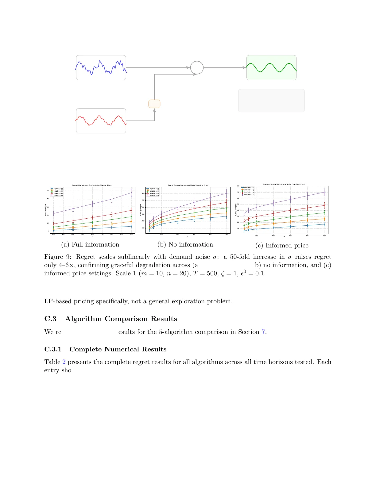
The V alue of Information in Resource-Constrained Pricing Ruic heng Ao † Jiash uo Jiang ‡ Da vid Simc hi-Levi † , § † Institute for Data, Systems, and So ciet y , Massac husetts Institute of T ec hnology § Departmen t of Civil and Environmen tal Engineering and Operations Research Cen ter, MIT aorc@mit.edu , dslevi@mit.edu ‡ Departmen t of Industrial Engineering and Decision Analytics, Hong Kong Universit y of Science and T echnology jsjiang@ust.hk Abstract Firms that price perishable resources—airline seats, hotel ro oms, seasonal inv en tory—no w routinely use demand predictions, but these predictions v ary widely in quality . Under hard ca- pacit y constrain ts, acting on an inaccurate prediction can irrev ersibly deplete inv en tory needed for future perio ds. W e study how prediction uncertaint y propagates into dynamic pricing de- cisions with linear demand, stochastic noise, and ﬁnite capacity . A certiﬁed demand forecast with kno wn error bound ϵ 0 sp eciﬁes where the system should op erate: it shifts regret from O ( √ T ) to O (log T ) when ϵ 0 ≲ T − 1 / 4 , and we prov e this threshold is tigh t. A misspeciﬁed surrogate mo del—biased but correlated with true demand—cannot set prices directly but re- duces learning v ariance b y a factor of (1 − ρ 2 ) through control v ariates. The tw o mechanisms comp ose: the forecast determines the regret regime; the surrogate tigh tens estimation within it. All algorithms rest on a b oundary attraction mechanism that stabilizes pricing near degen- erate capacity b oundaries without requiring non-degeneracy assumptions. Exp eriments conﬁrm the phase transition threshold, the v ariance reduction from surrogates, and robustness across problem instances. Keyw ords: Dynamic pricing, prediction uncertaint y , resource constraints, reven ue managemen t, demand learning, v alue of information. 1 In tro duction Firms that price perishable resources—airline seats, hotel rooms, cloud compute, seasonal in v en tory— no w routinely use demand predictions generated by mac hine learning mo dels, historical forecasting systems, or surrogate signals deriv ed from related mark ets. An airline may hav e a reven ue man- agemen t system calibrated ov er years of b o oking data; a cloud pro vider may use a demand mo del trained on workload traces from adjacen t services; a retailer entering a new market may rely on price-sensitivit y estimates transferred from a similar pro duct category . These predictions v ary widely in quality . A well-calibrated forecast ma y predict demand to within a few p ercent, while a surrogate trained on a diﬀeren t pro duct category captures broad price-sensitivit y patterns but carries systematic bias. The operational question is how pr e diction unc ertainty pr op agates into pricing de cisions when r esour c es ar e limite d and pricing err ors ar e irr eversible . This question arises b ecause demand predictions, how ev er sophisticated, are rarely exact. F ore- casting mo dels suﬀer from distributional shift as mark et conditions ev olv e; surrogate mo dels trained on oﬄine data ma y be misspeciﬁed relative to the current pricing en vironment; and ev en w ell- calibrated systems degrade when deplo y ed outside their training distribution. In unconstrained 1 settings, the consequences of prediction error are mild: a sub optimal price reduces reven ue for a single p erio d, and the ﬁrm can adjust in the next. Under hard capacity constrain ts, how ev er, the consequences are asymmetric and p otentially sev ere. Underpricing depletes inv en tory needed for the remainder of the selling horizon, and this depletion is irreversible. A pricing p olicy m ust there- fore simultaneously learn demand, exploit a v ailable predictions, and guard against the p ossibilit y that those predictions are wrong. This three-w a y tradeoﬀ—learning, earning, and hedging—has no analog in the unconstrained demand learning literature ( Keskin and Zeevi 2014 , Bu et al. 2020 ), where eac h p erio d’s pricing error is self-contained. Tw o practical observ ations motiv ate our approach. First, not all predictions are created equal: a forecast with a certiﬁed accuracy guaran tee carries fundamen tally diﬀerent information from a biased surrogate mo del, and a pricing system that treats them identically leav es v alue on the table or, w orse, destabilizes the system. Second, prediction quality in teracts with the time horizon in a non-ob vious wa y: a forecast that is adequate for a short selling season ma y b e dangerously inaccurate o v er a longer one. These observ ations suggest that the right framew ork should explicitly distinguish among prediction t yp es and c haracterize ho w prediction qualit y requiremen ts scale with the planning horizon. W e dev elop a uniﬁed framework for c onstr aine d dynamic pricing under pr e diction unc ertainty . Giv en predictions of unkno wn and heterogeneous qualit y , ho w should a capacit y-constrained ﬁrm decide which predictions to trust, how to use them, and when to discard them? W e distinguish tw o forms of prediction that en ter the problem diﬀerently: • A c ertiﬁe d demand for e c ast —a price-demand pair ( p 0 , d 0 ) with a known error bound ϵ 0 — sp eciﬁes wher e the system should op erate. When accurate enough, it shifts the regret regime from O ( √ T ) to O (log T ). • A missp e ciﬁe d surr o gate mo del —biased but correlated with true demand—cannot set prices directly but reduces estimation v ariance through con trol v ariates, accelerating learning within an y regime. These t w o roles are complemen tary and comp osable: the forecast determines what to do ; the surrogate determines how pr e cisely to le arn . Misusing either—trusting a biased surrogate as a price recommendation, or using an accurate forecast merely to reduce v ariance—forfeits reven ue or destabilizes the system. W e make three contributions. 1. Robust pricing under degeneracy (Section 3 ). W e introduce b oundary attraction, a re-solving mechanism that stabilizes pricing near degenerate capacit y boundaries. When resources approac h depletion or m ultiple pro ducts comp ete for the same capacity , the ﬂuid optimization that guides pricing admits m ultiple optimal solutions, and standard re-solving p olicies can oscillate b etw een them. b oundary attraction resolv es this b y rounding near-zero demand comp onen ts to zero, steering the system aw ay from the ill-conditioned region. With a calibrated demand mo del, the resulting p olicy ac hiev es O (log T ) regret without the non- degeneracy assumptions required b y prior analyses ( W ang and W ang 2022 , Li and Y e 2022 ). This mec hanism underlies all subsequent algorithms. 2. A prediction quality threshold for regime change (Sections 4 – 5 ). Without any forecast, our p olicy attains the minimax-optimal O ( √ T ) regret through p erio dic re-estimation and structured price p erturbations. With a certiﬁed forecast of accuracy ϵ 0 , a sharp phase transition emerges at ϵ 0 ≈ T − 1 / 4 : forecasts more accurate than this threshold recov er near- logarithmic regret, while less accurate forecasts are safely screened and the system rev erts 2 F ull Information Known ( α , B ) Informed Price Prior p 0 , error ϵ 0 No Information Online learning Surrogate Data Oﬄine auxiliary Inputs Step 1: Estimation Solve ﬂuid LP for target d ∗ Step 2: Boundary Attraction • Small demands: round to 0 • Large demands: keep safe Uniﬁed Algorithm Scenario A F ull Info / Go od Prior O (log T ) Scenario B No Info / P o or Prior O ( √ T ) Outcomes R e duces variance ϵ 0 ≈ T − 1 / 4 Figure 1: Ov erview of the uniﬁed framew ork. b oundary attraction underlies all settings. Without oﬄine information, the system learns online at the minimax O ( √ T ) rate. A certiﬁed informed price ( p 0 , d 0 ) can improv e the regime to near-logarithmic regret when ϵ 0 ≲ T − 1 / 4 , while correlated surrogate signals reduce learning v ariance and improv e constan ts. The com bined policy comp ounds b oth b eneﬁts. to online learning. F or a selling horizon of T = 10 , 000 p erio ds, this threshold corresp onds to roughly 10% prediction accuracy—a concrete target for forecast qualit y in v estmen t. A matc hing low er b ound (Prop osition 7 ) shows this threshold is tight: no algorithm can b eat Θ( √ T ) when ϵ 0 ≫ T − 1 / 4 , regardless of ho w it uses the forecast. 3. V ariance reduction from biased surrogates (Section 6 ). Missp eciﬁed surrogate models impro v e pricing when used as v ariance-reducing instrumen ts rather than direct recommen- dations. The mechanism is control v ariates: by subtracting the predictable component of demand noise using the correlated surrogate signal, the system obtains lo w er-v ariance pseudo- observ ations for parameter estimation. Surrogate correlation reduces the learning cost b y a factor of (1 − ρ 2 ), where ρ measures correlation with true demand. A surrogate with ρ = 0 . 7 reduces learning v ariance b y half; one with ρ = 0 . 9 reduces it b y 81%. Com bined with a certiﬁed forecast, the tw o mechanisms compose: the forecast shifts the regret regime, and the surrogate tigh tens estimation within it (Theorem 9 ). Across all settings, regret decomp oses in to three comp onents: sto chastic noise (inheren t demand v ariability), parameter uncertain t y (the cost of learning demand online), and initialization bias (the cost of prediction error). b oundary attraction controls the ﬁrst, surrogate correlation reduces the second, and forecast accuracy go verns the third. Figure 1 summarizes this decomp osition. 1.1 Related Literature Constrained pricing and degeneracy . Dynamic pricing of p erishable resources dates to the ﬂuid benchmark of Gallego and V an Ryzin ( 1994 ); see Jasin ( 2014 ), Bump ensanti and W ang ( 2020 ), W ang and W ang ( 2022 ), Jiang et al. ( 2025 ), Ao et al. ( 2024a , b , 2025b ), Jiang and Zhang ( 2025 ) 3 and references therein. Existing logarithmic-regret re-solving results require structural regularity— non-degeneracy or isolated optimal bases ( W ang and W ang 2022 , Li and Y e 2022 ). W e target the opp osite regime: ﬂuid solutions may b e degenerate exactly where capacity binds most tightly . b oundary attraction steers pricing aw a y from these ill-conditioned boundaries and delivers loga- rithmic regret without structural assumptions. Demand prediction and prior information in pricing. In unconstrained dynamic pricing, Keskin and Zeevi ( 2014 ) show that exact prior knowledge fundamentally improv es learning rates. Bu et al. ( 2020 ) c haracterize phase transitions and an in v erse-square la w for optimal regret as a function of oﬄine data qualit y , showing that even imp erfect historical prices carry non-trivial information. Subsequent work extends these ideas to oﬄine data integration and missp eciﬁcation ( F erreira et al. 2018 , W ang et al. 2024 , Li et al. 2021 , Simc hi-Levi and Xu 2022 , Xu and Zeevi 2020 ). A conference version of this pap er ( Ao et al. 2025a ) introduced the full-information, no- information, and informed-price settings under resource constraints, establishing that a certiﬁed prior in terpolates b et w een O (log T ) and O ( √ T ) regret. The presen t pap er extends that w ork in t w o directions: a matching low er b ound that pins the phase transition at ϵ 0 ≈ T − 1 / 4 (Prop osition 7 ), and surrogate-assisted v ariance reduction for biased but correlated prediction mo dels (Section 6 ). Theorem 9 shows these t w o mechanisms comp ose: the certiﬁed forecast determines the regret regime; the surrogate tigh tens estimation within it. Online learning under constrain ts. The bandits-with-knapsacks literature addresses on- line decision-making under resource constrain ts, primarily for discrete actions and bandit feedbac k ( Badanidiyuru et al. 2014 , Agraw al and Dev anur 2016 , Agra w al et al. 2016 , Liu et al. 2022 , Chen et al. 2024 , Ma et al. 2024 , Sank araraman and Slivkins 2021 , Siv akumar et al. 2022 , Liu and Grigas 2022 ). A separate line on learning-augmented algorithms studies consistency–robustness tradeoﬀs when external advice may b e imp erfect ( Lyk ouris and V assilvitskii 2021 , Mitzenmacher and V as- silvitskii 2022 , Purohit et al. 2018 , W ei and Zhang 2020 , Bhask ara et al. 2020 , 2021 , 2023 ). Our informed-price result follo ws the consistency–robustness logic but op erates in a diﬀerent decision structure: con tin uous pricing with ﬂuid LPs and irreversible resource consumption. Prediction-p o w ered inference and AI-assisted op erations. The surrogate framework builds on control v ariates and prediction-p o w ered inference ( Ao et al. 2026c , a , b ): the surrogate signal reduces estimation v ariance rather than directly recommending prices. This distinction matters under hard constraints, where biased price recommendations can trigger premature resource depletion but biased v ariance-reducing signals remain useful. More broadly , predictive systems and AI tools now provide decision supp ort across operational settings—from demand forecasting to optimization model formulation ( Liang et al. 2026 , Ao et al. 2026d , e , Duan et al. 2025 , Baek et al. 2026b , a ). W e characterize when such imp erfect predictions should alter the op erating p oin t (certiﬁed forecasts) and when they should only sharp en estimation (correlated surrogates). Notation. F or a real num ber x , we use ⌈ x ⌉ to denote the smallest in teger ≥ x and ⌊ x ⌋ for the largest in teger ≤ x . W e write x + = max { x, 0 } . F or a set S , let | S | b e its cardinality . W e denote b y d max = max p ∈ [ L,U ] n ∥ f ( p ) ∥ 2 the maxim um ℓ 2 -norm of an y feasible demand vector under the true demand function f . 2 Mo del and Preliminaries W e study dynamic pricing of n pro ducts sharing m resources ov er a horizon of T p erio ds. A t each p erio d t , the decision-maker (DM) sets a price v ector p t ∈ [ L, U ] n , observ es sto c hastic demand 4 d t ∈ R n + , and up dates remaining capacities b y c t +1 = c t − A d t , where A ∈ R m × n + is a kno wn consumption matrix and c 0 is the initial capacit y vector. The goal is to ﬁnd a pricing p olicy maximizing total exp ected reven ue E h T X t =1 ( p t ) ⊤ d t i , while resp ecting resource constrain ts (demand exceeding remaining capacity is not served). W e measure an y p olicy π b y its r e gr et relativ e to an idealized ﬂuid b enchmark that replaces random demand with its exp ectation and solves the resulting deterministic problem. Given a kno wn demand function f ( p ) = E [ d | p ], the ﬂuid optimal v alue is V Fluid ( c 0 ) = max p ∈ [ L,U ] n { T · p ⊤ f ( p ) | A f ( p ) ≤ c 0 /T } . (1) F ollowing the rev en ue managemen t literature ( T alluri and v an Ryzin 2004 , Bu et al. 2020 ), w e imp ose tw o structural assumptions: linear demand, whic h captures price sensitivit y with a ﬁnite-dimensional parameter space, and negative-deﬁnite slop e matrices, which guarantee concav e rev en ue and rule out pathological cases where low ering prices increases demand indeﬁnitely . Assumption 1 (Linear demand mo del) . We assume the true demand function is line ar. That is, ther e exist p ar ameters α = ( α 1 , . . . , α n ) ⊤ ∈ R n and B ∈ R n × n such that f ( p ) = α + B p for any pric e ve ctor p in the fe asible domain. Linear demand mo dels are standard in dynamic pricing ( Keskin and Zeevi 2014 , Jav anmard and Nazerzadeh 2019 ). Ev en in this setting, Bu et al. ( 2020 ) sho w that the interpla y b etw een oﬄine data and online learning pro duces rich phenomena—phase transitions and an inv erse-square la w— so linear demand is far from trivial when prior information quality v aries. Applications include airlines pricing p erishable seats, retailers selling seasonal go o ds, and cloud providers allocating compute capacity—all settings where unsold inv en tory has no salv age v alue. W e focus on linear demand for clarity; the analysis extends to general parametric mo dels under standard regularit y conditions (e.g., Lipsc hitz con tinuit y and conca vit y). Bey ond linearit y , we require the demand slop e to b e strictly negativ e-deﬁnite: Assumption 2 (Negative deﬁniteness) . The matrix B is ne gative deﬁnite; namely, λ max ( B + B ⊤ ) < 0 wher e λ max ( · ) denotes the lar gest eigenvalue of a matrix. We also assume that α is lar ge enough to guar ante e f ( p ) ≥ 0 for any pric e ve ctor p in the fe asible domain. This condition ensures strictly decreasing demand ( B j j < 0), in v ertibilit y of B , and conca vit y of the reven ue function p 7→ p ⊤ f ( p )—all essen tial for the b oundary attraction mechanism in Section 3 . The observ ed demand at p erio d t is d t = f ( p t ) + ϵ t , where ϵ t ∈ R n is a zero-mean noise vector with ϵ t ≥ − f ( p t ), assumed sub-Gaussian with parameter σ 2 : P ( | v ⊤ ϵ t | ≥ λ ) ≤ 2 exp( − λ 2 / (2 σ 2 )) for an y unit vector v . Reven ue at time t is r t = p t ⊤ d t 5 and resource consumption is A d t , so capacit y up dates as c t +1 = c t − A d t . If fulﬁlling demand d t for some pro duct would exhaust a resource, sales of that pro duct are curtailed to resp ect the capacit y constraint. W e w ork on a ﬁltered probabilit y space (Ω , F , {F t } T t =0 , P ) where F t enco des all information a v ailable up to time t . The ﬂuid b enc hmark upp er-b ounds the exp ected reven ue of any admissible p olicy: Prop osition 1 (( Gallego and V an Ryzin 1994 )) . F or any p olicy π , V Fluid ( c 0 ) ≥ E h T X t =1 ( p t ) ⊤ d t i . Th us V Fluid ( c 0 ) is a natural p erformance b enchmark. The r e gr et of a p olicy π ov er horizon T is Regret T ( π ) = V Fluid ( c 0 ) − E h T X t =1 ( p t ) ⊤ d t i . All p olicies solv e the same constrained control problem and diﬀer only in the demand informa- tion a v ailable. 3 Boundary A ttraction and F ull-Information Regret W e b egin with a calibrated demand prediction—the b est-case scenario where the ﬁrm’s forecast is exact—isolating the con trol diﬃcult y near hard capacity b oundaries b efore prediction error enters. The b oundary attraction mechanism dev eloped here is not merely a full-information b enchmark: it reapp ears as a subroutine in ev ery algorithm that follows, whether demand must b e learned from scratc h (Section 4 ), guided by a prior (Section 5 ), or assisted by surrogate data (Section 6 ). Ev en when the demand function f ( p ) = α + B p is kno wn, resource constraints force a nontrivial dynamic tradeoﬀ. A t each p erio d, the decision-mak er m ust balance immediate reven ue against future opp ortunit y: selling to o aggressively depletes resources needed later, while withholding in v en tory wastes p otential reven ue. Prior algorithms achiev e logarithmic regret by rep eatedly resolving the ﬂuid problem ( 1 ), but require strong non-degeneracy assumptions. F or instance, Jasin ( 2014 ) assumes the dual LP has a unique optimal vertex λ ∗ and that p erturbing the constraint righ t-hand side do es not change whic h constrain ts bind at optimalit y . W ang and W ang ( 2022 ) relaxes this to c 0  = T d ∗ ,T (the system is either ov erloaded or underloaded), but the regret b ound scales as Ω(   c 0 /T − d ∗ ,T   − 1 ). In practice, ho w ev er, degeneracy is perv asiv e ( Bump ensanti and W ang 2020 ): man y constraints bind sim ultaneously , and the optimal dual solution need not b e unique. Under degeneracy , near-zero optimal demands cause dual multipliers to div erge, making the system sensitiv e to small demand ﬂuctuations. W e address this through a b oundary attr action me chanism : whenever an optimal demand comp onent falls b elo w a dynamic threshold ζ ( T − t + 1) − 1 / 2 , w e round it to zero and push the corresponding price to ward its upp er bound U . This steers the system aw a y from the degenerate region at a mo dest cost of O ( ζ 2 log T ) additional regret (App endix D.1 ), while eliminating the unbounded dual v ariables that plague prior re-solving approac hes. 3.1 The Boundary Attraction Mechanism When the ﬂuid solution prescrib es near-zero demand d ∗ j ≈ 0 for some pro duct j , the corresp onding dual multiplier λ j ≈ 1 /d ∗ j div erges. T raditional re-solv e metho ds ( Jasin 2014 , W ang and W ang 6 Algorithm 1 Boundary Attracted Re-solve Metho d 1: Input: c 1 = C , A , f ( p ) = α + B p , rounding threshold ζ . 2: for t = 1 , . . . , T do 3: Solv e ﬂuid mo del ( 2 ) for ( p π ,t , d π ,t ) 4: Apply Boundary A ttraction: Set ˜ d t i = d π ,t i if d π ,t i ≥ ζ ( T − t + 1) − 1 / 2 , else 0 5: Set the candidate price ˆ p t = B − 1 ( ˜ d t − α ), then implemen t p t = Π [ L,U ] n ( ˆ p t ) 6: Observ e demand ˆ d t , up date c t +1 = c t − A ˆ d t 7: end for 2022 ) rely on ﬁrst-order corrections prop ortional to λ , which explo de under degeneracy . b oundary attraction resolves this by rounding small demands to zero. When d ∗ j < ζ ( T − t + 1) − 1 / 2 , we set ˜ d j = 0 and push the corresp onding price to its upp er b ound U , steering the system a w a y from regions where dual m ultipliers div erge. The attraction step truncates only near-zero demands, and the resulting loss is second-order in the truncated quan tit y; this yields a p er-p erio d loss of order O ( ζ 2 / ( T − t + 1)), whic h sums to O ( ζ 2 log T )—a logarithmic cost. The threshold deca ys as ( T − t + 1) − 1 / 2 : as the horizon shrinks, the algorithm tolerates progressiv ely smaller demands without rounding (Figure 5 in App endix B ). 3.2 Algorithm Design A t each p erio d, the algorithm pro ceeds in three steps: solv e the ﬂuid problem assuming no noise, ﬂag demands that fall below the threshold ζ ( T − t + 1) − 1 / 2 , and round those demands to zero while pricing the remaining pro ducts at the ﬂuid solution. The threshold decays as ( T − t + 1) − 1 / 2 b ecause sto chastic ﬂuctuations accum ulate at rate √ T − t + 1. A larger threshold reduces constrain t violations but increases rounding loss; a smaller one captures more rev en ue but risks infeasibilit y . F ormally , at eac h p erio d t , the DM observes the remaining capacities c t and solves the ﬂuid mo del: V Fluid t ( c t ) = max p ∈ [ L,U ] n p ⊤ d s.t. d = α + B p , A d ≤ c t T − t + 1 , (2) yielding an optimal solution ( p π ,t , d π ,t ). W e then round small demands to zero: ˜ d t i = ( d π ,t i if d π ,t i ≥ ζ ( T − t + 1) − 1 / 2 , 0 otherwise , and set the candidate price ˆ p t = B − 1 ( ˜ d t − α ). If ˆ p t lea v es the feasible b o x, w e clip it comp onent wise to obtain p t = Π [ L,U ] n ( ˆ p t ); clipping only aﬀects cases where the attraction step already pushes the solution tow ard the price b oundary . The ( T − t + 1) − 1 / 2 deca y rate matches the scale at which sto c hastic demand ﬂuctuations accumulate o ver the remaining horizon, yielding O ( ζ 2 log T ) regret under high-probabilit y concentration. When a resource is fully depleted ( c t i = 0), w e reject all future demand for pro ducts requiring that resource. 7 3.3 Regret Analysis The regret bound reﬂects three sources of loss—the rounding cost ( ζ 2 ), the dimension ( n 2 ), and the condition n um b er ∥ B − 1 ∥ 2 —all scaling with log T . Theorem 2. F or Algorithm 1 with ζ ≥ 4 σ 2 , the r e gr et is b ounde d by: Regret T  π  = O  ζ 2 n 2 ∥ B − 1 ∥ 2 log T  . The n 2 factor reﬂects the n × n entries of B , while ∥ B − 1 ∥ 2 captures ill-conditioning: large v alues indicate that demand resp onds sharply to price changes, amplifying p erturbation losses. Once the con trol lay er is stabilized, degeneracy no longer forces the analysis to rely on structural regularity assumptions. The pro of (App endix D.1 ) telescop es ov er hybrid p olicies. F or each p erio d t , a hybrid p olicy follo ws Algorithm 1 up to time t and then resolves optimally without noise for the remaining horizon. The k ey step b ounds the single-perio d reven ue diﬀerence E  R T ( Hybrid t , F T ) − R T ( Hybrid t +1 , F T )  . Because small demands d i ≈ 0 pro duce unbounded dual multipliers, we round them to zero pre- emptiv ely , moving the solution aw a y from degenerate b oundaries. The analysis splits into three cases by demand magnitude. F or large demand ( d i ≫ ( T − t + 1) − 1 / 2 ), standard concen tration inequalities suﬃce: the buﬀer region absorbs noise. F or small demand ( d i < ζ ( T − t + 1) − 1 / 2 ), b oundary attraction eliminates this case through rounding. F or mo derate demand, the second-order growth condition yields lo cally strong concavit y of reven ue, b ounding perturbation losses. Eac h perio d con tributes O ( ζ 2 n 2 ∥ B − 1 ∥ 2 /T ); summing ov er T perio ds yields the O (log T ) b ound. Unlike Jasin ( 2014 ) and W ang and W ang ( 2022 ), this approach requires no non-degeneracy assumptions and a voids ﬁrst-order correction terms. With this con trol mechanism in place, w e next study the cost of learning demand en tirely online. 4 Online Learning Without Prior Information W e no w consider the opp osite extreme: no demand prediction is av ailable, and the demand function m ust b e learned en tirely online. The algorithm inherits b oundary attraction from Section 3 and adds structured exploration. It also serves as the fallback p olicy when a forecast is to o unreliable to trust (Section 5 ). When the demand function f ( p ) = α + B p is unkno wn, the decision-mak er must sim ultaneously learn the parameters and set prices under resource constraints, balancing exploration (estimating α , B from price exp eriments) against exploitation (using current estimates to maximize reven ue)— the classical learning-earning tradeoﬀ. Resource constrain ts comp ound this tradeoﬀ: the contin- uous, high-dimensional state-action space makes dynamic programming in tractable, and capacity coupling across p erio ds creates path-dep enden t dynamics. Ensuring suﬃcien t exploration is the cen tral c hallenge. As Kes kin and Zeevi ( 2014 ) sho w, a m y opic policy that alwa ys prices at the curren t estimated optim um leads to incomplete learning and p o or rev en ue. F rom ( 10 ), estimation error scales inv ersely with λ min ( P t ), the minimum eigenv alue of the design matrix. This eigen v alue gro ws with the v ariance of historical prices (see ( 11 )), so if prices cluster to o tightly—alw a ys near the current estimate, for example—then λ min ( P t ) remains small and estimation stagnates. Our solution com bines p erio dic re-solving with controlled p erturbations. Every n p erio ds, w e re- estimate parameters and re-solv e the ﬂuid problem, adding a structured p erturbation σ 0 t − 1 / 4 e t − kn to the prices. Within each ep o ch, the p erturbations for t ∈ { k n + 1 , . . . , k n + n } ensure that the 8 diﬀerences p t − p t − 1 − X k form an orthogonal basis, where X k = ˜ p k − p kn anc hors the ep o ch. This orthogonalit y guaran tees λ min ( P t ) ≳ √ t , so estimation error decays at the optimal O ( t − 1 / 2 ) rate. The t − 1 / 4 p erturbation scale balances exploration against exploitation, yielding the √ T regret rate. 4.1 Algorithm Design Our approach combines ordinary least squares estimation on historical (price, demand) pairs, p eri- o dic re-solving ev ery n p erio ds with up dated estimates, and forced exploration through structured p erturbations to ensure price div ersit y . As noted ab o ve, estimation error scales inv ersely with λ min ( P t ) (see App endix A.2 for the full regression formulas, equations ( 9 )–( 10 ), and equation ( 11 )). T o guaran tee suﬃcient exploration, instead of directly using the ﬂuid-optimal price from V Fluid , we p erturb the pricing strategy p t to increase v ariance. Sp eciﬁcally , at time t , we set the desired price as ˜ p t = p t − 1 + ( ˜ p k − p kn ) + σ 0 t − 1 / 4 e t − kn for k = ⌊ ( t − 1) /n ⌋ , where ˜ p k solv es ( 2 ) with estimated parameters ˆ α kn +1 , ˆ B kn +1 and curren t in v en tory c kn +1 . The term ( ˜ p k − p kn ) acts as momentum tow ard the re-solve solution and anc hors prices for p erio ds k n + 1 , . . . , k n + n , balancing earning against learning. The temp oral structure of this p erio dic review pro cess is depicted in Figure 6 (App endix B ). App endix A.2 provides further design rationale. As in the full-information setting, b oundary attraction rejects demand for products whose predicted demand falls b elow a dynamic threshold. Here, the threshold ζ (( T − t + 1) − 1 / 4 + t − 1 / 4 ) has t w o terms, each addressing a distinct error source. The ( T − t + 1) − 1 / 4 term guards against sto c hastic demand ﬂuctuations accum ulating ov er the remaining horizon, while the t − 1 / 4 term accoun ts for estimation error, which deca ys as O ( t − 1 / 2 ) but requires an O ( t − 1 / 4 ) threshold for high-probabilit y feasibility . T ogether, the tw o terms ensure robustness: estimation error dominates early (small t ), while noise dominates late (large T − t ). 4.2 Regret Analysis Theorem 3. F or Algorithm 2 , with thr eshold ζ ≥ C n 5 / 4 log 3 / 2 nσ 0 √ σ log T for some c onstant C , the r e gr et is b ounde d by: Regret T  π  = O  ( ζ 2 + ∥ B − 1 ∥ 2 ) √ T  . Remark 1 (Optimalit y and special cases) . The O ( √ T ) r ate is minimax-optimal. Without r esour c e c onstr aints, i.e., setting A = 0 and c 0 = ∞ , we r e c over the unc onstr aine d dynamic pricing pr oblem of Keskin and Ze evi ( 2014 ), wher e the Ω( √ T ) lower b ound is tight. Our algorithm matches this limit despite the adde d c omplexity of r esour c e c onstr aints. The c o eﬃcient ( ζ 2 + ∥ B − 1 ∥ 2 ) sep ar ates two c osts: ζ 2 is the pric e of b oundary attr action for maintaining fe asibility, while ∥ B − 1 ∥ 2 me asur es how il l-c onditione d the demand mo del is. The or em 3 ther efor e char acterizes the worst-c ase c ost of le arning demand entir ely online. W e now sketc h the pro of of Theorem 3 ; full details app ear in App endix E.1 . Without loss of generalit y , assume T = nT ′ for some integer T ′ > 0. The ﬁrst step parallels the pro of of Theorem 2 : w e split the regret as Regret T  π  = E " T ′ X k =1 R T ( Hybrid k , F T ) − R T ( Hybrid k +1 , F T ) # , 9 Algorithm 2 Periodic-Review Re-solve with Parameter Learning 1: Input: Initial capacity c 1 = C , constraint matrix A , p erturbation scale σ 0 , threshold ζ . 2: for t = 1 , . . . , n do 3: Sample p t uniformly from [ L, U ] n to initialize exploration. 4: end for 5: Compute initial av erage price p n = 1 n P n t =1 p t . 6: for t = n + 1 , . . . , T do 7: if mo d ( t, n ) = 1 then 8: Set blo c k index k = ⌊ ( t − 1) /n ⌋ . 9: Estimate ˆ α kn +1 and ˆ B kn +1 using regression on historical data. 10: Solv e the estimated ﬂuid mo del with current capacity c kn +1 to obtain ˜ p k . 11: end if 12: Set price p t = p t − 1 + ( ˜ p k − p kn ) + σ 0 t − 1 / 4 e t − kn . 13: Compute predicted demand ˜ d t = ˆ α kn +1 + ˆ B kn +1 p t . 14: Deﬁne rejection set I t r = { i ∈ [ n ] : ˜ d t i ≤ ζ (( T − t + 1) − 1 / 4 + t − 1 / 4 ) } . 15: Observ e actual demand ˆ d t = f ( p t ) + ϵ t , and reject demands in I t r . 16: Up date capacit y c t +1 = c t − A ˆ d t . 17: Up date a v erage price p t = t − 1 t p t − 1 + 1 t p t . 18: end for where R T ( Hybrid k , F T ) denotes the total rev enue of the hybrid p olicy deﬁned as using Algorithm 2 up to time k n and getting the remaining reven ue by solving ( 2 ) directly without noise. Unlik e in Theorem 2 , the true parameters and ﬂuid-optimal solutions are unav ailable. W e must therefore b ound the estimation error of ˆ α kn +1 , ˆ B kn +1 relativ e to α , B . A stabilit y result for strongly concav e constrained programs ( Bonnans and Shapiro 2013 , Prop. 4.32) implies that Dist  ˆ d , D π ,t  is b ounded linearly by    B − ˆ B    2 + ∥ α − ˆ α ∥ 2 . The structured p erturbations ensure λ min ( P t ) ≳ √ t via ( 11 ), so the parameter error decays at rate O ( t − 1 / 2 ). Combining this with the noise analysis from Theorem 2 yields the ﬁnal b ound. W e provide a matching low er b ound: the O ( √ T ) rate is optimal up to constant factors; more- o v er, this holds for any giv en tuple of problem parameters. F ormally , Keskin and Zeevi ( 2014 ) establish that ev en in the unconstrained case, Lemma 4 ( Keskin and Zeevi 2014 ) . Ther e exists a ﬁnite p ositive c onstant c > 0 such that Regret T  π  ≥ c √ T for any online p olicy π . This lo w er b ound applies a fortiori to our resource-constrained setting, since dropping the constrain ts can only reduce regret. Theorem 3 is therefore rate-optimal. This b enchmark clariﬁes what oﬄine information must b eat. W e next study the informed-price setting, where a certiﬁed prior observ ation can aﬀect the operating p oin t itself; Section 6 then turns to surrogate information, whic h instead improv es estimation. 5 Informed Prices with Error Certiﬁcation Bet w een calibrated demand and complete ignorance lies a practically important middle ground: the ﬁrm has a demand forecast ( p 0 , d 0 ) from historical op erations, a pilot study , or a predictive mo del, with a certiﬁed error b ound ∥ d 0 − f ( p 0 ) ∥ 2 ≤ ϵ 0 . W e call such a forecast a c ertiﬁe d anchor . 10 An accurate anchor can c hange the regret regime b ecause it changes the op erating p oin t itself. Under hard capacity constraints, how ev er, that also makes it dangerous when wrong. If the anchor is accurate, we should approac h the logarithmic p erformance of the full-information b enc hmark; if it is inaccurate, we should not do w orse than O ( √ T ). The central question is therefore not whether the anc hor helps in principle, but when it is accurate enough to trust. This interpolation exhibits a sharp phase transition at ϵ 0 ≈ T − 1 / 4 , driv en by t wo comp eting error sources. If the algorithm trusts the informed price but the observ ation is inaccurate, the resulting bias accumulates as O (( ϵ 0 ) 2 T ); if it instead learns from scratc h, the cost of learning is O ( √ T ). The transition o ccurs where these t w o costs balance: ( ϵ 0 ) 2 T ≈ √ T ⇒ ϵ 0 ≈ T − 1 / 4 . Belo w this threshold ( ϵ 0 < T − 1 / 4 ), exploiting the informed price yields O (log T ) regret. Ab ov e it ( ϵ 0 > T − 1 / 4 ), learning from scratc h at rate O ( √ T ) is preferable. F or a typical horizon of T = 10 , 000 p erio ds, the threshold is ϵ 0 ≈ 0 . 1—meaning the forecast m ust predict demand to within 10% accuracy to unlo ck logarithmic regret. In v esting in b etter demand prediction pa ys oﬀ only if the forecast error can b e driven b elow this T − 1 / 4 threshold. What makes the informed price usable is c ertiﬁc ation : kno wing ϵ 0 . Without this information, an algorithm cannot determine ho w m uc h to trust the anc hor v ersus con tin uing to explore. Any algorithm that lac ks this certiﬁcate cannot achiev e b etter than Θ( √ T ) worst-case regret. 5.1 Wh y Error Certiﬁcation Is Necessary Without kno wing ϵ 0 , an algorithm faces a dilemma: trust the anchor (risking that bias from the wrong mo del accum ulates ov er time) or learn from scratch (forgoing the p otential b eneﬁt of a go o d prior). Unable to resolv e this dilemma, an y such algorithm must hedge, achieving only Θ( √ T ) w orst-case regret. Prop osition 5. Ther e exist p ar ameter sets ( α, B ) and ( α ′ , B ′ ) such that, for any p olicy π lacking know le dge of ϵ 0 , if π achieves r e gr et O ( T γ ) for some γ ∈ (0 , 1) on ( α, B ) , it incurs r e gr et Ω( T 1 − γ ) on ( α ′ , B ′ ) . The pro of (see Appendix F ) constructs t w o adversarial instances indistinguishable from ( p 0 , d 0 ): in the ﬁrst, ϵ 0 is small and the optimal algorithm exploits the anchor to achiev e O (log T ); in the second, ϵ 0 is large and the optimal algorithm learns from scratc h at rate O ( √ T ). Since ( p 0 , d 0 ) lo oks identical in b oth cases, any algorithm without knowledge of ϵ 0 ac hiev es Θ( √ T ) (see Figure 7 in App endix B for a visualization of this decision logic). The same logic underlies the consistency-robustness tradeoﬀ in learning-augmen ted algorithms ( Lyk ouris and V assilvitskii 2021 , Mitzenmacher and V assilvitskii 2022 ): to b eat the baseline using predictions, one must know the prediction quality . Here, the anc hor ( p 0 , d 0 ) pla ys the role of the prediction, and ϵ 0 quan tiﬁes its qualit y . 5.2 Algorithm Design Giv en ϵ 0 , w e implemen t a consistency-robustness switch. First, we chec k whether ( ϵ 0 ) 2 T > τ √ T for a tuning parameter τ . If this condition holds, the informed price is to o noisy to trust, so we rev ert to Algorithm 2 (the no-information p olicy). Otherwise, w e anchor estimation at ( p 0 , d 0 ) and exploit the certiﬁed prior. 11 Algorithm 3 Certiﬁed-Anchor Estimate-then-Select Re-solve 1: Input: Initial capacity c 1 = C , matrix A , error b ound ϵ 0 , tolerance τ , p erturbation scale σ 0 , threshold ζ . 2: if ( ϵ 0 ) 2 T > τ √ T then 3: Switc h to Algorithm 2 (no-information setting). 4: end if 5: for t = 1 , . . . , T do 6: Compute ˆ B t using regression anc hored at ( p 0 , d 0 ). 7: Solv e the estimated ﬂuid mo del ˆ V Fluid t ( c t ) with ˆ B t and c t . 8: P erturb the solution: ˜ p t ← ˜ p t + σ 0 sgn( ˜ p t − p 0 ) t − 1 / 2 e mod ( t,n ) . 9: Compute predicted demand ˜ d t = d 0 + ˆ B t ( ˜ p t − p 0 ). 10: Deﬁne rejection set I t r = { i ∈ [ n ] : ˜ d t i ≤ ζ (( T − t + 1) − 1 / 2 + t − 1 / 2 ) } . 11: Observ e ˆ d t = f ( ˜ p t ) + ϵ t , reject demands in I t r , and up date c t +1 = c t − A ˆ d t . 12: end for W e estimate B using ( p 0 , d 0 ) as a reference p oin t: ˆ B t = t − 1 X s =1 ( p s − p 0 )( p s − p 0 ) ⊤ ! † t − 1 X s =1 ( d s − d 0 )( p s − p 0 ) ⊤ . (3) This centering remo v es the in tercept term α , reducing the estimation problem from ( n + 1) × n parameters to n × n . When ϵ 0 is small, d 0 ≈ α + B p 0 , so this approach yields accurate estimates of B with few er samples. W e still add small perturbations σ 0 t − 1 / 4 sgn( ˜ p t − p 0 ) e mod ( t,n ) to ensure suﬃcien t exploration, but these decay faster than in the no-information case. The directional term sgn( ˜ p t − p 0 ) p erturbs aw a y from the informed price p 0 —up w ard when the ﬂuid solution exceeds p 0 , do wn w ard otherwise—exploiting the reference p oint for faster conv ergence when ϵ 0 is small. 5.3 Regret Analysis Theorem 6. F or Algorithm 3 , the r e gr et is b ounde d by: Regret T  π  = O  min n τ √ T , ( ϵ 0 ) 2 T + ( ζ 2 + ∥ B − 1 ∥ 2 ) σ 2 log T o . Theorem 6 quantiﬁes the v alue of the informed price. Unlik e the surrogate signals studied in Section 6 , a certiﬁed anchor can improv e the regret regime itself b ecause it c hanges the op erating p oin t rather than only the estimator. The ﬁrst term, τ √ T , is the robust fallback from the no- information setting. The second term captures the b eneﬁt and risk of trusting the anchor: the initial error ϵ 0 con tributes a bias of order ( ϵ 0 ) 2 T , while the logarithmic term is the same sto c hastic cost presen t in the full-information b ound. When ϵ 0 = 0, we reco v er O (log T ) (full-information); as ϵ 0 increases past T − 1 / 4 , the b ound con v erges to O ( √ T ) (no-information). This in terp olation is tigh t: Prop osition 7. Ther e exist instanc es wher e any p olicy without know le dge of ϵ 0 incurs r e gr et Ω(max { τ √ T , ( ϵ 0 ) 2 T } ) , matching the upp er b ound in The or em 6 . T ogether, these results iden tify exactly when prior information can change the op erating p oint: only when the anc hor is certiﬁed tightly enough to b eat the learning baseline. W e next turn to surrogate mo dels, which should not set prices directly but can still reduce the statistical cost of learning. 12 6 V ariance Reduction via Surrogate Mo dels The certiﬁed forecast of Section 5 requires a prediction accurate enough to change the op erating p oin t. W e now study a weak er but more common form of prediction. Firms routinely maintain demand mo dels based on historical data, customer features, and con textual signals. Such mo dels ma y b e to o biased to set prices directly , but they can still reduce the v ariance of online estimation through their correlation with true demand. The role of a surrogate is indirect: it impro v es the estimator, not the action. W e sho w that oﬄine surr o gate mo dels , despite p otential bias or missp eciﬁcation, can reduce estimation v ariance and improv e the constants in the O ( √ T ) regret b ound. W e do not require the surrogate to b e un biased or even to preserve the ranking of demands across prices. The key requirement is merely informative c orr elation : the surrogate predictions m ust b e non-trivially correlated with the true demand. 6.1 Problem Setup and Oﬄine Surrogate Mo del Prior to deplo ymen t, the ﬁrm has collected an oﬄine dataset D oﬀ = { z i } N i =1 of side information (e.g., customer features, context v ariables) that do es not include realized demand under the candidate prices P = { p (1) , . . . , p ( K ) } ⊂ [ L, U ] n . A pre-existing predictive model provides a demand surrogate S d ( z , p ) ∈ R n , trained oﬄine on historical data from a diﬀerent pricing p olicy . Here z denotes observ able side information at deploymen t time (e.g., demographics, seasonalit y , traﬃc patterns). The framework accommo dates missp eciﬁcation: the surrogate may systematically ov er- or un- derestimate demand. W e correct for bias by centering (subtracting the surrogate’s mean via oﬄine data) and applying control v ariates (using the centered surrogate to reduce v ariance, not to predict directly). F ormally , w e allow the surrogate to be biase d — E [ S d ( z t , p t )]  = E [ d t | p t ]—and require only informative c orr elation : Assumption 3 (Informativ e correlation) . F or e ach pric e p ∈ P , the surr o gate S t ( p ) := S d ( z t , p ) and the demand d t satisfy Cov ( d t , S t ( p ) | p t = p )  = 0 . In addition, the surr o gate c ovarianc e matrix is non-de gener ate: Σ S ( p ) := V ar ( S t ( p ) | p t = p ) ≻ 0 , ∀ p ∈ P . This condition ensures that the surrogate carries non-trivial information ab out demand ﬂuctu- ations, ev en if the mean is misaligned, and that the con trol-v ariate co eﬃcient Γ ⋆ ( p ) is well-deﬁned. W e also require a quasi-uniform oﬄine cov erage condition (App endix G.1 ), guaranteeing that the oﬄine price design co v ariance is b ounded aw a y from singularity; this is the standard richness con- dition for MLA estimation. Remark 2 (How muc h correlation suﬃces?) . V arianc e r e duction V ar eﬀ ≈ (1 − ρ 2 ) V ar implies: ρ = 0 . 5 yields 25% r e duction, ρ = 0 . 7 yields 49%, and ρ = 0 . 9 yields 81%. Exp eriments (Se ction 7 ) show that me aningful r e gr et r e duction ( > 5% ) r e quir es ρ ≥ 0 . 5 . Surr o gates with ρ < 0 . 3 pr ovide ne gligible b eneﬁt and may not justify deployment overhe ad. 6.2 V ariance Reduction via Con trol V ariates W e adapt classical control v ariates: giv en a correlated v ariable X with known mean, the estimator ˜ Y = Y − β ( X − E [ X ]) is unbiased with reduced v ariance when X and Y are correlated. Applying 13 this to ( d t , S t ( p t )) pairs, let ˇ S t ( p ) denote a c enter e d v ersion of the surrogate, obtained b y subtracting an oﬄine reference mean: ˇ S t ( p ) := S t ( p ) − ¯ m ( p ) , where ¯ m ( p ) is an estimate of the surrogate mean E [ S t ( p )] computed from the oﬄine dataset D oﬀ . The centered surrogate ˇ S t ( p ) has approximately zero mean when av eraged ov er the oﬄine distri- bution, enabling v ariance reduction. F or a given price p t , w e deﬁne the pseudo-observation e d t := d t − Γ( p t ) ˇ S t ( p t ) , (4) where Γ( p ) ∈ R n × n is a matrix that linearly combines the demand and the centered surrogate. The v ariance of e d t (conditionally on p t = p ) is minimized when Γ ⋆ ( p ) = Σ dS ( p ) Σ S ( p ) − 1 , where Σ dS ( p ) := Co v( d t , S t ( p ) ⊤ | p t = p ) is the cross-co v ariance and Σ S ( p ) := V ar( S t ( p ) | p t = p ) is the surrogate’s co v ariance matrix. With this optimal choice, the v ariance of the pseudo-observ ation is giv en b y the Schur c omplement : V ar( e d t | p t = p ) = Σ d ( p ) − Σ dS ( p )Σ S ( p ) − 1 Σ S d ( p ) , (5) whic h is strictly smal ler than the original demand v ariance Σ d ( p ) whenever Σ dS ( p )  = 0 and Σ S ( p ) ≻ 0 (by Assumption 3 ). See Figure 8 in App endix B for a conceptual ov erview of this v ariance reduction pro cess. This is the residual v ariance after remo ving the comp onent of d t predictable from S t ( p ). F or the special case of scalar targets (e.g., rev en ue r t = p ⊤ t d t ), the v ariance reduction simpliﬁes to V ar( e r t | p t = p ) = σ 2 r ( p )(1 − ρ ( p ) 2 ), where ρ ( p ) := Corr( r t , S t ( p ) | p t = p ); see App endix G.2 for a w ork ed n umerical example. 6.3 Surrogate-Assisted An ytime Regression Estimating the control v ariate co eﬃcien t. W e estimate the surrogate mean m ⋆ ( p ) and the co eﬃcien t Γ ⋆ via regularized regression. Under a linear kernel, the estimator reduces to regularized OLS with feature dimension D feat ≈ n , ensuring estimation error of order O ( n log T ) that preserv es the optimal regret rate: b Γ t := b Σ dS,t ( b Σ oﬀ S + λI ) − 1 , (6) where λ > 0 is a regularization parameter. An ytime OLS with pseudo-observ ations. At time t , the DM forms the pseudo-observ ation e d t := d t − b Γ t ( p t ) ˇ S t ( p t ) and then applies standard ordinary least squares (OLS) to estimate ( α , B ). Sp eciﬁcally , for eac h pro duct j = 1 , . . . , n , let x s = [1; p s ] ∈ R 1+ n and P t = P t s =1 x s x ⊤ s . The estimator is " b α t j b β t j # = ( P t ) − 1 t X s =1 " e d s j e d s j p s # , b B t := [ b β t 1 , . . . , b β t n ] ⊤ . (7) This surrogate-assisted OLS replaces the raw demand d s in the baseline no-information algorithm (Algorithm 2 ) with the v ariance-reduced pseudo-observ ation e d s . 14 6.4 Regret analysis The estimation error has t w o comp onen ts: an or acle varianc e ﬂo or Va r orc (the Sch ur complement ( 5 ), irreducible even with the true Γ ⋆ ) and an empiric al error from the plug-in b Γ t ( p ) diﬀering from Γ ⋆ ( p ) due to ﬁnite samples and centering mismatch. Unlik e a certiﬁed prior, surrogate assistance t ypically do es not c hange the regret regime b y itself; it low ers the v ariance within the O ( √ T ) learning rate. Theorem 8 (Regret with Surrogate Assistance) . Consider Algorithm 2 mo diﬁe d to use surr o gate- assiste d pseudo-observations ( 4 ) in the OLS estimator ( 7 ) . Supp ose the r esiduals ( d t − µ d ( p t ) , S t ( p t ) − m ⋆ ( p t )) ar e jointly Gaussian with c ovarianc e matrix  Σ d ( p ) Σ dS ( p ) Σ S d ( p ) Σ S ( p )  for e ach p , and let the of- ﬂine surr o gate data satisfy a quasi-uniform c over age c ondition (detaile d in App endix G.1 ). Under the p ar ametric assumption that the c ontr ol variate c o eﬃcient Γ ⋆ ( p ) is c onstant and m ⋆ ( p ) is line ar, the exp e cte d r e gr et satisﬁes E [ R e gr et T ( π )] = O  ( ζ 2 + ∥ B − 1 ∥ 2 ) ·  σ eﬀ √ T + n log T + nT N  , (8) wher e σ 2 eﬀ := sup p λ max (Σ d ( p ) − Σ dS ( p )Σ S ( p ) − 1 Σ S d ( p )) is the or acle varianc e fr om the Schur c om- plement ( 5 ) . The term n log T + nT N ac c ounts for estimating the c ontr ol variate c o eﬃcient and c entering. The leading term σ eﬀ √ T is the oracle regret ﬂoor—strictly smaller than the baseline O ( q σ 2 d · T ) in Theorem 3 b y a factor of p 1 − ρ 2 in the scalar case. The remaining terms n log T + nT / N capture the cost of estimating the control v ariate parameters and centering; these are negligible when N ≫ √ T . Theorem 8 shows that biased surrogates help by shrinking the learning v ariance rather than by directly selecting prices. The pro of follo ws the framework of Theorem 3 but replaces σ 2 d with V a r orc in the self-normalized concen tration step; see App endix G.1 for the complete argument and App endix G.2 for a pro of sk etch. Informed priors and surrogates are complemen tary but not in terc hangeable. A certiﬁed prior can improv e the regret regime when reliable enough; a surrogate uses abundan t but p oten tially missp eciﬁed oﬄine data to impro v e the constan t in the learning term. In practice, priors suit settings where a trust worth y benchmark is av ailable with quantiﬁable error, while surrogates suit settings where oﬄine data is plen tiful but its quality is uncertain. 6.5 Surrogate-assisted informed pricing The t w o forms of oﬄine information can b e com bined: the certiﬁed prior impro v es the regime, while the surrogate shrinks the learning term inside that regime. W e now combine the informed-price approac h of Section 5 with the surrogate assistance developed ab ov e. Consider the setting where the ﬁrm uses the surrogate mo del to construct an initial informed price p 0 and demand estimate d 0 = E [ S d ( z , p 0 )]. If the surrogate’s bias is bounded b y ϵ 0 , i.e., ∥ E [ S d ( z , p 0 )] − f ( p 0 ) ∥ 2 ≤ ϵ 0 , we can adapt the Estimate-then-Select strategy (Algorithm 3 ) to use surrogate-assisted estimation. Theorem 9 (Regret with Surrogate and Informed Prior) . Consider A lgorithm 3 wher e the OLS estimator is r eplac e d by the surr o gate-assiste d estimator ( 7 ) anchor e d at ( p 0 , d 0 ) . The exp e cte d r e gr et satisﬁes: E [ R e gr et T ( π )] = O  min n σ eﬀ √ T , ( ϵ 0 ) 2 T + ( ζ 2 + ∥ B − 1 ∥ 2 )( σ 2 + σ 2 eﬀ ) log T o + n 2 log T + n 2 T N  . 15 Theorem 9 stacks the tw o b eneﬁts. If the anchor is to o biased ( ϵ 0 large), the p olicy falls back to a surrogate-assisted O ( σ eﬀ √ T ) learning regime. If the anc hor is accurate ( ϵ 0 small), we retain logarithmic regret. Comparing with Theorem 6 , the sto chastic noise component is unc hanged, while the learning comp onent improv es from σ 2 to σ 2 eﬀ —a reduction b y the ratio σ 2 eﬀ /σ 2 < 1. The additiv e terms n 2 log T + n 2 T / N capture the cost of learning the surrogate relationship in the anc hored matrix-v alued regression step; these are negligible when N ≫ T / log T . Discussion. The Sch ur complement formula ( 5 ) sho ws that correlation matters more than ac- curacy: a high-correlation, mo derately biased surrogate outp erforms a lo w-correlation, low-bias predictor. The framew ork therefore applies whenev er ﬁrms main tain predictiv e mo dels trained on historical or auxiliary data, even under distributional shifts and mo del missp eciﬁcation (see App endix G.2 for further discussion). 7 Numerical Exp erimen ts W e v alidate the theoretical predictions through sim ulated pricing exp eriments, examining regret scaling across information regimes, the phase transition in the informed-price setting, and the v ariance reduction from surrogate signals. Exp erimen tal setup. W e use tw o problem scales. Scale 1 ( m = 10 resources, n = 20 pro d- ucts) has suﬃcient dimensionality to exhibit asymptotic regret scaling ( O (log T ) versus O ( √ T )) while remaining computationally tractable. Scale 2 ( m = 1 resource, n = 4 pro ducts) permits extensiv e replication (500 runs p er conﬁguration), whic h reduces standard errors enough to detect p erformance diﬀerences b et w een algorithms. W e generate random instances as follows. The consumption matrix A ∈ R m × n + has en tries dra wn i.i.d. from Uniform[0 , 1]. Demand parameters are sampled with α i ∼ Uniform[5 , 10] and B ij ∼ Uniform[ − 1 , 0]. T o satisfy Assumption 2 , we shift the diagonal entries of B by subtracting the largest eigen v alue of ( B + B ⊤ ) / 2. Initial capacities are c 0 = Ad ∗ , where d ∗ = arg max d ≥ 0 d ⊤ B − 1 ( d − α ) is the unconstrained optimal demand. This ensures resource constraints activ ely bind under optimal pricing. W e add i.i.d. Gaussian observ ation noise N (0 , σ 2 ) and set p erturbation scale σ 0 = 1 for all algorithms. Unless stated otherwise, w e use threshold parameter ζ = 1, noise lev el σ = 1, and (for informed-price algorithm) initial error ϵ 0 = 0 . 1. App endix C lists all exp erimental parameters. Regret scaling v alidation. W e ﬁrst verify that regret scales according to the theoretical pre- dictions (Scale 1: m = 10, n = 20). Figure 2 plots regret against the time horizon T ∈ { 50 , 100 , 200 , 400 , 800 , 1600 } for the full-information, no-information, and informed-price settings, with σ = 1 and ϵ 0 = T − 1 / 2 in the informed case. Eac h p oint av erages 100 indep endent runs; error bars sho w ± 1 standard deviation. The observed rates matc h the theory . F ull-information regret (Figure 2 a) grows as O (log T ): it stays nearly constant across horizons—the cost of sto chastic constraint managemen t alone. No- information regret (Figure 2 b) scales as O ( √ T ), matching the minimax rate. Informed-price regret (Figure 2 c) with ϵ 0 = T − 1 / 2 ≪ T − 1 / 4 sta ys nearly ﬂat, conﬁrming the phase transition predicted b y Theorem 6 : when the initial estimate is accurate enough, regret drops from O ( √ T ) to O (log T ). These patterns are robust across randomly generated instances. Regret gro ws linearly in the noise standard deviation σ but remains sub quadratic ev en when σ increases 50-fold (App endix C ). On instances where all ﬂuid-optimal demands are b ounded a w a y from zero, the b oundary attraction 16 threshold ζ has little eﬀect: p erformance is stable across ζ ∈ [0 . 5 , 2] and degrades only at ζ ≥ 5 (App endix C.2.2 ). When some demand comp onents are near zero, ho w ever, b oundary attraction with ζ ∈ [1 , 3] sharply reduces regret from demand-ﬂo or bias (App endix C.2.2 ). 0 200 400 600 800 1000 1200 1400 1600 T i m e h o r i z o n T 20 10 0 10 20 Regret ( a ) F u l l I n f o r m a t i o n : O ( l o g T ) a + b l o g T f i t Full Information 0 200 400 600 800 1000 1200 1400 1600 T i m e h o r i z o n T 10000 20000 30000 40000 50000 60000 70000 80000 90000 ( b ) L e a r n i n g : O ( p T ) a + b p T f i t Learning (No Info) 0 200 400 600 800 1000 1200 1400 1600 T i m e h o r i z o n T 14000 15000 16000 17000 18000 ( c ) I n f o r m e d P r i c i n g : O ( l o g T ) a + b l o g T f i t Informed Pricing Figure 2: Regret scaling across time horizons T conﬁrms theoretical predictions: (a) full information gro ws as O (log T ), (b) no information scales as O ( √ T ), and (c) informed price with ϵ 0 = T − 1 / 2 reco v ers near-logarithmic regret. Com bining informed prices and surrogate assistance. W e next quantify ho w informed prices and oﬄine surrogates con tribute, individually and join tly . W e compare ﬁve algorithms on Scale 2 ( m = 1 resource, n = 4 pro ducts) with 500 replications p er conﬁguration: (i) F ull-Information (Oracle): Algorithm 1 with kno wn demand model, serving as a lo w er b ound on ac hiev able regret. (ii) Surrogate+Informed : Algorithm 3 augmen ted with surrogate-assisted estimation (Sec- tion 6 ). (iii) Informed Price : Algorithm 3 with initial error ϵ 0 = 0 . 12. (iv) Surrogate : Algorithm 2 with surrogate-assisted estimation (Section 6 ). (v) Learning (Baseline): Algorithm 2 with no prior information. W e set σ = 2 . 2 and surrogate correlation ρ = 0 . 65. Figure 3 plots regret tra jectories across T ∈ { 200 , 400 , 600 , 800 , 1000 } . T able 1 rep orts results at T = 200. The ranking Learning > Surrogate > Informed > Surro- gate+Informed is consistent across replications. The tw o information channels are complementary: com bining them reduces regret b elow either channel alone, the surrogate reduces estimation v ari- ance (Section 6 ) while the informed anc hor reduces bias (Section 5 ). As T grows, the gap b etw een algorithms widens (Figure 3 ); complete results across all horizons app ear in App endix C.3 . V alue of informed prices. Theorem 6 predicts a phase transition at ϵ 0 ≈ T − 1 / 4 : b elo w this threshold, regret grows as O (( ϵ 0 ) 2 T + log T ); ab ov e it, the informed observ ation is to o noisy to help and regret rev erts to O ( √ T ). Figure 4 conﬁrms the prediction: for eac h T , mean regret (300 replications) rises from the log T ﬂo or through the quadratic regime and saturates at the √ T ceiling. The transition sharp ens with T , and the inﬂection p oints cluster near ϵ 0 ≈ T − 1 / 4 (see also Figure 11 in App endix C.4 ). 17 T able 1: Algorithm p erformance comparison at T = 200 (500 replications, Scale 2: m = 1, n = 4, σ = 2 . 2). Algorithm Mean Regret F ull-Information (Oracle) 7 . 31 ± 81 . 6 Surrogate+Informed 303 . 91 ± 112 . 7 Informed Price 328 . 61 ± 112 . 4 Surrogate 452 . 69 ± 191 . 9 Learning (Baseline) 530 . 36 ± 227 . 0 V alue of surrogate assistance. The control-v ariate construction of Section 6 reduces estimation v ariance b y a factor (1 − ρ 2 ), where ρ is the correlation b et ween surrogate and true demand. Because the reduction dep ends on correlation alone—not on mean or slope accuracy—missp eciﬁed surrogates with ρ > 0 still help. With N = 500 oﬄine observ ations and 20% parameter missp eciﬁcation, regret decreases monotonically with ρ (Figure 12 in App endix C.4 ), matching the (1 − ρ 2 ) prediction. 8 Conclusions This pap er studies ho w prediction uncertaint y propagates into constrained dynamic pricing. Our framew ork separates the problem in to three la yers: stabilizing pricing near degenerate capacit y b oundaries (boundary attraction), determining when a forecast is reliable enough to shift the regret regime (the phase transition at ϵ 0 ≈ T − 1 / 4 ), and extracting v alue from biased predictions through v ariance reduction rather than direct price recommendation. The results pro duce a clear hierarch y: O ( √ T ) regret without predictions, O (log T ) with an ac- curate forecast, and a (1 − ρ 2 ) v ariance reduction factor from correlated surrogates that comp ounds with either regime. The phase transition threshold is tight—no algorithm can impro v e on O ( √ T ) when ϵ 0 ≫ T − 1 / 4 —giving a precise answ er to when a demand forecast is worth trusting. F or practitioners, the operational guidelines are concrete: set the boundary attraction threshold conserv atively ( ζ ∈ [1 , 5]); trust a demand forecast only when its error b ound is on the order of T − 1 / 4 or smaller; and use surrogate mo dels as v ariance-reducing instrumen ts, not price recommendations, with gains b ecoming substan tial around ρ ≥ 0 . 5. The analysis assumes linear demand. Three extensions would broaden applicabilit y: certifying prediction reliability when ϵ 0 is not known a priori, extending the framework to nonlinear or con textual demand models, and exploiting richer surrogate structures—such as neural netw ork sim ulators—while preserving constrain t feasibility . References Abbasi-Y adkori Y, P´ al D, Szep esv´ ari C (2011) Impro v ed algorithms for linear sto chastic bandits. A dvanc es in neur al information pr o c essing systems 24. Agra wal S, Dev anur N (2016) Linear contextual bandits with knapsacks. A dvanc es in neur al information pr o c essing systems 29. Agra wal S, Dev an ur NR, Li L (2016) An eﬃcient algorithm for contextual bandits with knapsac ks, and an extension to conca ve ob jectives. Confer enc e on L e arning The ory , 4–18 (PMLR). Ao R, Chen H, Gao S, Li H, Simc hi-Levi D (2026a) Best arm iden tiﬁcation with llm judges and limited h uman. arXiv pr eprint arXiv:2601.21471 . 18 250 500 750 1000 1250 1500 1750 2000 T i m e h o r i z o n T 0 500 1000 1500 2000 2500 Regret A l g o r i t h m C o m p a r i s o n ( m = 1 , n = 4 , σ = 2 . 2 ) O ( p T ) r e f Full Information Surrogate+Informed Informed Pricing Surrogate-Assisted Learning (No Info) Figure 3: Regret tra jectories for the ﬁv e algorithms on Scale 2 ( m = 1, n = 4, σ = 2 . 2, 500 replications). Shaded regions show ± 1 standard deviation. Combining b oth information channels (Surrogate+Informed) yields the lo w est regret; the separation b etw een algorithms grows with T . Ao R, Chen H, Gao S, Li H, Simchi-Levi D (2026b) Designing service systems from textual evidence. arXiv pr eprint arXiv:2603.10400 . Ao R, Chen H, Liu H, Simc hi-Levi D, Sun WW (2026c) Ppi-svrg: Unifying prediction-p ow ered inference and v ariance reduction for semi-sup ervised optimization. arXiv pr eprint arXiv:2601.21470 . Ao R, Chen H, Simchi-Levi D, Zhu F (2024a) Online lo cal false discov ery rate con trol: A resource allo cation approac h. arXiv pr eprint arXiv:2402.11425 . Ao R, F u H, Simchi-Levi D (2024b) Tw o-stage online reusable resource allo cation: Reserv ation, ov erbo oking and conﬁrmation call. arXiv pr eprint arXiv:2410.15245 . Ao R, Jiang J, Simchi-Levi D (2025a) Learning to price with resource constraints: from full information to mac hine-learned prices. The Thirty-ninth A nnual Confer enc e on Neur al Information Pr o c essing Systems . Ao R, Luo G, Simchi-Levi D, W ang X (2025b) Optimizing llm inference: Fluid-guided online scheduling with memory constrain ts. URL . Ao R, Simchi-Levi D, W ang X (2026d) Optirepair: Closed-lo op diagnosis and repair of supply chain opti- mization mo dels with llm agents. arXiv pr eprint arXiv:2602.19439 . Ao R, Simchi-Levi D, W ang X (2026e) Solver-in-the-loop: Mdp-based b enc hmarks for self-correction and b eha vioral rationalit y in op erations research. arXiv pr eprint arXiv:2601.21008 . Badanidiyuru A, Langford J, Slivkins A (2014) Resourceful contextual bandits. Confer enc e on L e arning The ory , 1109–1134 (PMLR). Baek J, Chen Y, Chi Z, Ma W (2026a) Ev aluating llm-p ersona generated distributions for decision-making. arXiv pr eprint arXiv:2602.06357 . Baek J, F u Y, Ma W, Peng T (2026b) Ai agen ts for in ven tory control: Human-llm-or complementarit y . arXiv pr eprint arXiv:2602.12631 . Bhask ara A, Cutkosky A, Kumar R, Purohit M (2020) Online linear optimization with many hints. URL https://arxiv.org/abs/2010.03082 . 19 1 0 2 1 0 1 1 0 0 I n i t i a l e r r o r b o u n d ² 0 500 1000 1500 2000 2500 3000 3500 4000 Regret O ( ( ² 0 ) 2 T + l o g T ) O ( p T ) ² 0 ≈ T − 1 / 4 T = 4 0 0 T = 8 0 0 T = 1 6 0 0 T = 3 2 0 0 Figure 4: Phase transition in informed-price regret (300 replications p er p oin t; error bars: ± 1 SE). Belo w ϵ 0 ≈ T − 1 / 4 (dashed v ertical), regret sta ys near the O (log T ) ﬂoor; ab o ve it, regret rises to the O ( √ T ) baseline (dashed horizontal). The transition sharp ens with T , consistent with Theorem 6 . Bhask ara A, Cutkosky A, Kumar R, Purohit M (2021) Logarithmic regret from sublinear hints. URL https: //arxiv.org/abs/2111.05257 . Bhask ara A, Cutk osky A, Kumar R, Purohit M (2023) Bandit online linear optimization with hints and queries. Krause A, Brunskill E, Cho K, Engelhardt B, Sabato S, Scarlett J, eds., Pr o c e e dings of the 40th International Confer enc e on Machine L e arning , volume 202 of Pr o c e e dings of Machine L e arning R ese ar ch , 2313–2336 (PMLR), URL https://proceedings.mlr.press/v202/bhaskara23a.html . Bonnans JF, Shapiro A (2013) Perturb ation analysis of optimization pr oblems (Springer Science & Business Media). Bo yd S, V anden b erghe L (2004) Convex optimization (Cambridge universit y press). Bu J, Simchi-Levi D, Xu Y (2020) Online pricing with oﬄine data: Phase transition and inv erse square law. International Confer enc e on Machine L e arning , 1202–1210 (PMLR). Bump ensan ti P , W ang H (2020) A re-solving heuristic with uniformly bounded loss for netw ork rev enue managemen t. Management Scienc e 66(7):2993–3009. Chen Z, Ai R, Y ang M, Pan Y, W ang C, Deng X (2024) Contextual decision-making with knapsacks b ey ond the worst case. The Thirty-eighth Annual Confer enc e on Neur al Information Pr o c essing Systems , URL https://openreview.net/forum?id=Dgt6sh2ruQ . Cheung WC, Lyu L (2024) Leveraging (biased) information: Multi-armed bandits with oﬄine data. arXiv pr eprint arXiv:2405.02594 . Duan Y, Hu Y, Jiang J (2025) Ask, clarify , optimize: Human-llm agent collab oration for smarter in v entory con trol. arXiv pr eprint arXiv:2601.00121 . F erreira KJ, Simc hi-Levi D, W ang H (2018) Online net work rev en ue management using thompson sampling. Op er ations r ese ar ch 66(6):1586–1602. Gallego G, V an Ryzin G (1994) Optimal dynamic pricing of inv en tories with sto chastic demand ov er ﬁnite horizons. Management scienc e 40(8):999–1020. Jasin S (2014) Reoptimization and self-adjusting price control for netw ork reven ue management. Op er ations R ese ar ch 62(5):1168–1178. 20 Ja v anmard A, Nazerzadeh H (2019) Dynamic pricing in high-dimensions. Journal of Machine L e arning R ese ar ch 20(9):1–49. Jiang J, Ma W, Zhang J (2025) Degeneracy is ok: Logarithmic regret for netw ork reven ue managemen t with indiscrete distributions. Op er ations R ese ar ch . Jiang J, Zhang M (2025) An lp-based approach for bilinear saddle p oint problem with instance-dep endent guaran tee and noisy feedback. Available at SSRN 5465554 . Keskin NB, Zeevi A (2014) Dynamic pricing with an unknown demand mo del: Asymptotically optimal semi-m yopic p olicies. Op er ations r ese ar ch 62(5):1142–1167. Lattimore T, Szep esv´ ari C (2020) Bandit algorithms (Cam bridge Universit y Press). Li X, Y e Y (2022) Online linear programming: Dual conv ergence, new algorithms, and regret b ounds. Op er ations R ese ar ch 70(5):2948–2966. Li Y, Xie H, Lin Y, Lui JC (2021) Unifying oﬄine causal inference and online bandit learning for data driv en decision. Pr o c e e dings of the Web Confer enc e 2021 , 2291–2303. Liang K, Lu Y, Mao J, Sun S, Y ang C, Zeng C, Jin X, Qin H, Zhu R, T eo CP (2026) Large-scale opti- mization mo del auto-form ulation: Harnessing llm ﬂexibility via structured workﬂo w. arXiv pr eprint arXiv:2601.09635 . Liu H, Grigas P (2022) Online con textual decision-making with a smart predict-then-optimize method. arXiv pr eprint arXiv:2206.07316 . Liu S, Jiang J, Li X (2022) Non-stationary bandits with knapsacks. A dvanc es in Neur al Information Pr o- c essing Systems 35:16522–16532. Lyk ouris T, V assilvitskii S (2021) Comp etitive caching with machine learned advice. Journal of the ACM (JA CM) 68(4):1–25. Ma W, Xia D, Jiang J (2024) High-dimensional linear bandits with knapsacks. International Confer enc e on Machine L e arning , 34008–34037 (PMLR). Mitzenmac her M, V assilvitskii S (2022) Algorithms with predictions. Communic ations of the A CM 65(7):33– 35. Purohit M, Svitkina Z, Kumar R (2018) Impro ving online algorithms via ml predictions. A dvanc es in Neur al Information Pr o c essing Systems 31. Sank araraman KA, Slivkins A (2021) Bandits with knapsacks b ey ond the worst case. A dvanc es in Neur al Information Pr o c essing Systems 34:23191–23204. Simc hi-Levi D, Xu Y (2022) Bypassing the monster: A faster and simpler optimal algorithm for contextual bandits under realizabilit y . Mathematics of Op er ations R ese ar ch 47(3):1904–1931. Siv akumar V, Zuo S, Banerjee A (2022) Smo othed adversarial linear contextual bandits with knapsac ks. International Confer enc e on Machine L e arning , 20253–20277 (PMLR). T alluri KT, v an Ryzin GJ (2004) The The ory and Pr actic e of R evenue Management (New Y ork: Springer). V era A, Banerjee S (2021) The bay esian prophet: A low-regret framew ork for online decision making. Man- agement Scienc e 67(3):1368–1391. V ershynin R (2018) High-Dimensional Pr ob ability: An Intr o duction with Applic ations in Data Scienc e . Cam bridge Series in Statistical and Probabilistic Mathematics (Cambridge Universit y Press), URL http://dx.doi.org/10.1017/9781108231596 . W ainwrigh t MJ (2019) High-dimensional statistics: A non-asymptotic viewp oint , v olume 48 (Cambridge univ ersity press). W ang Y, W ang H (2022) Constant regret resolving heuristics for price-based rev en ue management. Op er ations R ese ar ch 70(6):3538–3557. W ang Y, Zheng Z, Shen ZJM (2024) Online pricing with p olluted oﬄine data. Available at SSRN 4320324 . W ei A, Zhang F (2020) Optimal robustness-consistency trade-oﬀs for learning-augmented online algorithms. A dvanc es in Neur al Information Pr o c essing Systems 33:8042–8053. Xu Y, Zeevi A (2020) Upp er counterfactual conﬁdence b ounds: a new optimism principle for contextual bandits. arXiv pr eprint arXiv:2007.07876 . 21 A Extended In tuitions A.1 Boundary A ttracted Re-solve Metho d Boundary attraction serv es three purp oses. First, it preven ts noise-induced constraint violations b y creating a buﬀer zone near resource depletion. Second, it enables single-step regret analysis without non-degeneracy conditions: by a v oiding the near-zero instabilit y region, w e b ound per- p erio d regret indep enden tly (App endix D.1 ). Third, the safety margin absorbs b oth stochastic noise (full-information setting) and parameter estimation errors (learning settings), providing uniform robustness across all prediction qualit y regimes. A.2 V ariance Perturbation and Anc horing OLS regression form ulas. Giv en historical data ( p 1 , d 1 ) , . . . , ( p t − 1 , d t − 1 ), w e deﬁne D t j := t − 1 X s =1 [ d s j ; d s j · p s ] ⊤ , ∀ j ∈ [ n ] , P t :=  t − 1 P t − 1 s =1 ( p s ) ⊤ P t − 1 s =1 p s P t − 1 s =1 p s ( p s ) ⊤  . (9) The OLS estimator is then " ˆ α t j ˆ β t j # = ( P t ) † D t j =  α j β j  + ( P t ) † " P t − 1 s =1 ϵ s j P t − 1 s =1 ϵ s j · p s # , ∀ j ∈ [ n ] , (10) where ( P t ) † denotes the pseudo-inv erse of P t . The estimation error scales inv ersely with the smallest eigen v alue of P t . F ollowing Keskin and Zeevi ( 2014 ), denoting p t = t − 1 P t s =1 p s , one can show that λ min ( P t ) ≥ 1 n (1 + 2 U 2 ) n ⌊ t/n ⌋ X s =1 (1 − 1 s )   p s − p s − 1 − X ⌈ s/n ⌉   2 2 (11) for some ﬁxed anchor X k , k = 0 , 1 , . . . , suc h that p s − p s − 1 − X k , s = k n + 1 , . . . , k n + n form an orthogonal basis of R n . This b ound shows that λ min ( P t ) gro ws with the accumulated v ariance of historical prices—exactly what the structured p erturbations in Algorithm 2 maximize. P erturbation design. In line 12 of Algorithm 2 , we add controlled exploration noise to the price: p t = p t − 1 + ( ˜ p k − p kn ) + σ 0 t − 1 / 4 e t − kn (12) where e t − kn ∼ N (0 , I n ) is a standard Gaussian v ector. This p erturbation serves tw o purp oses: 1. Exploration : prices all products with enough v ariation for accurate regression-based param- eter estimation. 2. V ariance control : the t − 1 / 4 deca y rate explores aggressiv ely early (when estimation error ∥ ˆ B kn +1 − B ∥ is large) and exploits later (when estimates tigh ten). This forced exploration tec hnique adapts standard contextual-bandit approac hes ( Abbasi-Y adkori et al. 2011 ) to our p erio dic re-solving structure. 22 Anc horing regression with informed prices. When an informed price-demand pair ( p 0 , d 0 ) with kno wn error b ound ϵ 0 is a v ailable, w e anc hor the regression on this prior while adapting to newly observ ed data. A t time t , we solve the constrained least squares problem: min α,B t − 1 X s =1 ∥ d s − ( α + B p s ) ∥ 2 2 sub ject to ∥ d 0 − ( α + B p 0 ) ∥ 2 2 ≤ ϵ 2 0 . (13) This form ulation is closely related to the unconstrained regression in Xu and Zeevi ( 2020 ) and Simc hi-Levi and Xu ( 2022 ), and extends to multiple informed prices by solving min α,B t − 1 X s =1 ∥ d s − ( α + B p s ) ∥ 2 2 sub ject to ∥ d 0 ,i − ( α + B p 0 ,i ) ∥ 2 2 ≤ ϵ 2 0 ,i , ∀ ( p 0 ,i , d 0 ,i ) . Wh y not estimate ϵ 0 online A natural question is whether ϵ 0 could be learned adaptiv ely during the selling horizon. In our setting, testing the informed price m ultiple times to estimate ϵ 0 p ermanen tly depletes capacit y , prev en ting future corrections. Unlik e unconstrained settings, exploration here has p ermanent costs. As Prop osition 7 suggests, this cost can make the informed- price algorithm p erform w orse than algorithms that ignore the oﬄine data entirely . B Conceptual Figures This app endix collects the conceptual diagrams referenced in the main text. C Numerical Exp erimen ts: Conﬁguration, Results, and Analysis This app endix pro vides parameter sp eciﬁcations, robustness analysis, complete algorithm compar- isons, and statistical v alidation for the exp eriments in Section 7 . C.1 Exp erimen tal Conﬁguration W e test on tw o problem scales: Scale 1 ( m = 10 resources, n = 20 pro ducts) and Scale 2 ( m = 1, n = 4). F or eac h scale, random instances are drawn as follows. Consumption matrix en tries A ij are i.i.d. Uniform[0 , 1]; demand in tercepts α j ∼ Uniform[5 , 10]; and price-sensitivity entries B j k ∼ Uniform[ − 1 , 0]. T o enforce Assumption 2 , w e shift B ← B − λ max  B + B ⊤ 2  I n , ensuring negativ e deﬁniteness. Initial capacity is set to c 0 = A d ∗ , where d ∗ is the unconstrained optimal demand, so that resource constrain ts bind at the ﬂuid optimum. Observed demand at each p erio d is ˜ d t = d ( p t ) + ξ t with ξ t ∼ N (0 , σ 2 I n ). Unless otherwise stated, all algorithms use b oundary attraction threshold ζ = 1, p erturba- tion scale σ 0 = 1, and conﬁdence level 1 − δ with δ = 0 . 05 (see Section 4 for conﬁdence region construction). 23 d 1 d 2 Capacit y Ad = c/T ζ / √ τ ζ / √ τ Fluid Opt (Safe) Boundary A ttraction F orces tiny demand → 0 ■ Danger Zone ■ Safe Zone — Constraint Figure 5: Sc hematic of the b oundary attraction mec hanism in Algorithm 1 . The red shaded regions represen t the danger zone where resource degeneracy causes instabilit y: when a demand comp onen t falls b elow threshold ζ ( T − t + 1) − 1 / 2 , dual v ariables can div erge. Fluid solutions in this region are rounded to the b oundary (zero demand), ensuring dual v ariables remain b ounded and the re-solve p olicy main tains stabilit y . C.2 Robustness Analysis C.2.1 Robustness to Demand Noise Figure 9 shows algorithm robustness across v arying demand noise levels, testing each information setting with noise standard deviation σ ∈ { 0 . 1 , 0 . 2 , 0 . 5 , 1 , 2 , 5 } (k eeping ζ = 1 and ϵ 0 = 0 . 1 ﬁxed, using Scale 1: m = 10, n = 20, T = 500). All three algorithms remain stable as noise increases by t w o orders of magnitude. F rom σ = 0 . 1 to σ = 5, regret increases only mo destly , conﬁrming that the algorithms degrade gracefully under demand uncertain t y rather than failing abruptly . Robustness across noise lev els: All three algorithms exhibit sublinear scaling with noise. Comparing σ = 0 . 1 to σ = 5 (a 50-fold increase), full-information regret increases 6-fold (5 to 30), no-information regret increases 4-fold (200 to 800), and informed-price regret increases 5-fold (10 to 50). This sublinear growth conﬁrms eﬀectiv e noise tolerance. All algorithms main tain their relativ e ranking across noise lev els, so the p erformance ordering is robust to mis-sp eciﬁcation of σ . 24 Time t 0 n 2 n 3 n Ep o ch 0 (Burn-in) Ep o ch 1 Ep o ch 2 Random Pricing (Gather Initial Data) Structured Perturbation p t = Anchor + Noise t Reﬁned Perturbation (Decaying Scale) UP UP UP Update Phase (UP): 1. OLS Est. ( ˆ α, ˆ B ) 2. Solve Fluid LP → New Anchor 3. Reset Basis Exploration Mechanism: Perturbations σ 0 t − 1 / 4 en- sure min eigenv alue λ min ( P t ) ↑ . Figure 6: Timeline of Algorithm 2 . The horizon is divided into epo chs of length n . A t each up date p oin t (UP), parameters are re-estimated via ordinary least squares and the ﬂuid plan is re-optimized. Within ep o chs, structured p erturbations σ 0 t − 1 / 4 e t − kn ensure the design matrix has eigen v alues growing at rate Ω( √ t ). Input: Prior ( p 0 , d 0 ) , Error Bound ϵ 0 Check Quality: ( ϵ 0 ) 2 T ≤ τ √ T ? Algorithm 3 (T rust) · Anchor OLS at ( p 0 , d 0 ) · Exploit lo w bias Result: O (log T ) Regret Algorithm 2 (F allback) · Discard inaccurate prior · Explore from scratch Result: O ( √ T ) Regret Uniﬁed Outcome Achieves optimal min { Bias , Variance } trade-oﬀ YES (Small ϵ 0 ) NO (Large ϵ 0 ) Phase Transition Threshold: ϵ 0 ≈ T − 1 / 4 Figure 7: Decision logic for Algorithm 3 . The algorithm chec ks whether the initial error b ound ϵ 0 falls b elow the phase transition threshold ≈ T − 1 / 4 . When the prior is accurate (left branch), the algorithm anchors estimation at ( p 0 , d 0 ) and achiev es O (log T ) regret; when inaccurate (right branc h), it rev erts to full exploration and achiev es O ( √ T ) regret. C.2.2 Eﬀect of Threshold P arameter ζ Figure 10 shows ho w the threshold parameter ζ (used in boundary attraction, Algorithm 1 ) impacts p erformance across ζ ∈ { 0 , 1 , 2 , 5 , 10 } , with σ = 1 and ϵ 0 = 0 . 1 ﬁxed (using Scale 1: m = 10, n = 20, T = 500). The sharp regret increase from ζ = 0 to ζ = 1 (3–5 × w orse at ζ = 0) reveals wh y b ound- ary attraction matters: without thresholding, the algorithm b ecomes trapp ed at degenerate solu- tions where inﬁnitesimal price changes pro duce negligible demand signal. Setting ζ = 1 requires ˜ d j ( p t ) ≥ ζ σ b efore selling pro duct j , forcing exploration at prices that pro duce meaningful signal and breaking degeneracy . Beyond ζ ≈ 1–2, gains diminish b ecause o v er-thresholding reduces the eﬀectiv e exploration signal. A mo derate v alue ζ ∈ [1 , 2] balances these t w o forces. P erformance stabilizes across ζ ∈ [0 . 5 , 2], indicating robustness to mo derate v ariations. Bey ond ζ ≥ 5, ov er-ﬁltering reduces the eﬀectiv e sample size and degrades p erformance. The optimal v alue ζ ≈ 1 emerges consistently across all three information regimes. The eﬀect is most pronounced for full-information and informed-price algorithms, which rely hea vily on solving the ﬂuid LP . This conﬁrms that b oundary attraction addresses degeneracy in 25 Online Observ ation ( d t ) V ariance = σ 2 Oﬄine Surrogate ( S t ) Correlated, Biased − × Γ Control V ariate Pseudo-Observ ation ( ˜ d t ) V ar ≈ (1 − ρ 2 ) σ 2 Mec hanism: Subtracting the predictable noise com- ponent (Γ S t ) isolates the true signal. Figure 8: Concept of Surrogate-Assisted V ariance Reduction . Correlated oﬄine surrogate signals S t act as con trol v ariates. By subtracting the predictable component of the noise (Γ S t ) from the ra w online demand d t , w e obtain a low er-v ariance pseudo-observ ation ˜ d t for estimation. 200 300 400 500 600 700 800 900 1000 T 0 10 20 30 40 50 A verage R egr et R egr et Comparison A cr oss Noise Standar d Er r or noise_std = 0.1 noise_std = 0.5 noise_std = 1.0 noise_std = 2.0 noise_std = 5.0 (a) F ull information 200 400 600 800 1000 T 300 400 500 600 700 800 A verage R egr et R egr et Comparison A cr oss Noise Standar d Er r or noise_std = 0.1 noise_std = 0.5 noise_std = 1.0 noise_std = 2.0 noise_std = 5.0 (b) No information 200 400 600 800 1000 T 10 20 30 40 50 60 70 80 A verage R egr et R egr et Comparison A cr oss Noise Standar d Er r or noise_std = 0.1 noise_std = 0.5 noise_std = 1.0 noise_std = 2.0 noise_std = 5.0 (c) Informed price Figure 9: Regret scales sublinearly with demand noise σ : a 50-fold increase in σ raises regret only 4–6 × , conﬁrming graceful degradation across (a) full information, (b) no information, and (c) informed price settings. Scale 1 ( m = 10, n = 20), T = 500, ζ = 1, ϵ 0 = 0 . 1. LP-based pricing sp eciﬁcally , not a general exploration problem. C.3 Algorithm Comparison Results W e rep ort the complete results for the 5-algorithm comparison in Section 7 . C.3.1 Complete Numerical Results T able 2 presents the complete regret results for all algorithms across all time horizons tested. Eac h en try sho ws mean regret ± standard deviation based on 500 replications. Bold entries indicate the b est learning algorithm (excluding the F ull-Info oracle) at each time horizon T . A t T = 200, algorithms that exploit more prediction information achiev e lo w er regret: Surro- gate+Informed < Informed < Surrogate < Learning. This ordering p ersists across all time horizons, consisten t with the theoretical predictions. 26 200 300 400 500 600 700 800 900 1000 T 0 20 40 60 80 100 120 140 160 A verage R egr et R e g r e t C o m p a r i s o n A c r o s s T h r e s h o l d = 0 = 1 = 2 = 5 = 1 0 (a) F ull information 200 400 600 800 1000 T 0 2000 4000 6000 8000 10000 12000 14000 A verage R egr et R egr et Comparison A cr oss Thr eshold = 0 = 1 = 2 = 5 = 1 0 (b) No information 200 400 600 800 1000 T 40 60 80 100 120 140 160 A verage R egr et R e g r e t C o m p a r i s o n A c r o s s T h r e s h o l d = 0 = 1 = 2 = 5 = 1 0 (c) Informed price Figure 10: Remo ving b oundary attraction ( ζ = 0) increases regret 3–5 × ; mo derate v alues ζ ∈ [1 , 2] stabilize p erformance across (a) full information, (b) no information, and (c) informed price settings. Scale 1 ( m = 10, n = 20), T = 500, σ = 1, ϵ 0 = 0 . 1. T able 2: Complete regret results across all time horizons. Mean ± standard deviation (500 repli- cations). T F ull-Info Surr+Inf Informed Surrogate Learning 200 − 0 . 06 ± 81 . 8 103 . 99 ± 99 . 3 170 . 18 ± 99 . 3 388 . 40 ± 89 . 2 662 . 94 ± 442 . 3 400 − 9 . 14 ± 123 . 6 57 . 99 ± 135 . 5 160 . 49 ± 125 . 9 508 . 68 ± 136 . 8 990 . 17 ± 841 . 6 600 2 . 19 ± 160 . 8 0 . 20 ± 167 . 5 160 . 09 ± 149 . 8 593 . 41 ± 186 . 3 1314 . 75 ± 1189 . 3 800 − 6 . 47 ± 199 . 4 − 60 . 51 ± 213 . 5 143 . 63 ± 201 . 9 660 . 50 ± 196 . 3 1554 . 92 ± 1524 . 4 1000 13 . 22 ± 207 . 5 − 85 . 66 ± 275 . 0 125 . 18 ± 235 . 7 742 . 22 ± 410 . 2 1738 . 40 ± 1722 . 5 C.4 Additional Exp erimen tal Results Figures 11 and 12 supplemen t the main text (Section 7 ) with results on the missp eciﬁcation–horizon tradeoﬀ and surrogate correlation, resp ectiv ely . D Pro ofs for Boundary A ttraction (F ull Information) This section formalizes the full-information setting: the ﬁrm kno ws the exact demand mo del f ( p ) = α + B p . The main diﬃcult y is controlling resource constraints under noisy demand realizations while main taining logarithmic regret. The b oundary attraction Mec hanism. Our analysis uses b oundary attraction to con- trol degeneracy in constrained optimization. When estimated demands d π ,t i fall b elow a dynamic threshold ζ ( T − t + 1) − 1 / 2 , w e round them to zero rather than risk infeasibilit y due to noise. This buﬀer preven ts the algorithm from hov ering near degenerate regions—states where some pro duct demands approac h zero and the ﬂuid optimization problem has m ultiple optimal solutions. Un- lik e prior w ork ( W ang and W ang 2022 , Li and Y e 2022 ) requiring non-degeneracy assumptions throughout (i.e., min i d ∗ i ≥ δ > 0 for some problem-dep endent constant δ ), our mechanism pro- duces b oundary-attracted decisions that mo v e small co ordinates on to safe reduced-dimensional faces. This eliminates the need for restrictiv e assumptions while paying only an O ( ζ 2 log T ) cost for conserv ative rounding, thereby preserving the logarithmic regret rate. 27 0 500 1000 1500 2000 2500 3000 T 0 2000 4000 6000 8000 10000 12000 14000 R egr et R e g r e t v s T f o r D i f f e r e n t 0 V a l u e s ( I n f o r m e d ) eps0=0 eps0=0.1 eps0=0.2 eps0=0.5 eps0=1 eps0=2 eps0=5 eps0=10 Figure 11: Phase transition in the informed-price setting: regret shifts from O (log T ) to O ( √ T ) as ϵ 0 crosses the threshold ≈ T − 1 / 4 . D.1 Pro of of Theorem 2 Pro of Roadmap W e establish the O (( n 2 ζ 2 + σ 2 ) ∥ B − 1 ∥ 2 log T ) regret b ound through the follow- ing steps: 1. Hybrid Policy Construction: Deﬁne a sequence of hybrid p olicies { Hybrid t } T +1 t =1 that in- terp olate b et ween the oﬄine optimal solution and our online algorithm, enabling a telescoping decomp osition of regret. 2. Single-Step Diﬀerence Analysis: Decomp ose the total regret into a sum of single-step diﬀerences R T (Hybrid t , F T ) − R T (Hybrid t +1 , F T ) and analyze eac h term independently . Our h ybrid p olicy decomp osition is inspired b y the comp ensated coupling technique of V era and Banerjee ( 2021 ), but diﬀers in tw o k ey asp ects: (1) w e handle contin uous pricing decisions rather than discrete accept/reject c hoices, where the most critical “correct / incorrect de- cision” analysis in their setting no longer holds; (2) our b oundary attraction mec hanism explicitly prev en ts degeneracy , whereas prior dynamic pricing pap ers assume non-degeneracy throughout. 3. Case-b y-Case Bounding via boundary attraction: F or eac h time p erio d, classify in to three cases based on the magnitude of estimated demands relativ e to the rounding threshold ζ : • Case I : All demands large (no rounding) — control rev en ue loss via noise concentration • Case I I : All demands small (full rounding) — show rounding cost is negligible • Case I I I : Mixed demands — combine techniques from Cases I and I I 4. Concen tration Inequalities: Apply sub-Gaussian tail b ounds to control the probability that noise causes constrain t violations or large deviations from the ﬂuid b enchmark. 5. Summation and Final Bound: Sum the p er-p erio d b ounds ov er all T p erio ds, sho wing that the logarithmic term is driv en by conserv ativ e rounding and intrinsic sto chasticit y . 28 0.0 0.2 0.4 0.6 0.8 Sur r ogate Cor r elation 13000 14000 15000 16000 17000 A verage R egr et R egr et R eduction with Sur r ogate Assistance (m=10, n=20, T=500) Baseline (No Sur r ogate) Sur r ogate- Assisted Figure 12: Surrogate v ariance reduction tracks the theoretical prediction (1 − ρ 2 ): at ρ = 0 . 9, observ ed regret drops 21% versus 19% predicted. Con trast with prior w ork. T raditional approaches ( W ang and W ang 2022 , Li and Y e 2022 ) require min i d ∗ i ≥ δ > 0 to hold glob al ly throughout the horizon—a restrictiv e assumption that fails when resources approach depletion or m ultiple pro ducts comp ete for the same capacity . boundary attraction adjusts dynamically: when the ﬂuid optimal solution suggests small demands (below threshold ζ ( T − t + 1) − 1 / 2 ), we round them to zero, pa ying only O ( ζ 2 / ( T − t )) per p erio d. Summing o v er all p erio ds yields O ( ζ 2 log T ) total cost. The threshold ζ ( T − t + 1) − 1 / 2 balances t wo forces: larger ζ increases the safet y buﬀer (reducing constrain t violations) but increases rounding cost; smaller ζ allo ws more aggres siv e pricing but risks infeasibility . Setting ζ = Θ( σ √ log n ) achiev es the optimal trade-oﬀ, eliminating the problem-dep enden t constant δ from the regret b ound. D.1.1 Step 1: Problem Setup and Hybrid P olicy Construction Problem F ormulation. At each time t , the algorithm solves the follo wing re-solve constrained programming problem: max p ∈P r = p ⊤ d s.t. d = α + B p , Ad ≤ c t T − t + 1 , (14) where c t is the inv en tory lev el at the b eginning of time t , and ( p π ,t , d π ,t ) denotes the optimal solution. Notation. T o streamline the exp osition, we introduce the following notation: • p ( d ) := B − 1 ( d − α ): in v erse demand function mapping demand to price • r ( d ) := p ( d ) ⊤ d : rev en ue as a function of demand (without noise) • r ( d , ϵ ) := r ( d ) + p ( d ) ⊤ ϵ : rev en ue when actual demand is d + ϵ • R T ( π ′ , F T ): total reven ue under p olicy π ′ giv en realized sample path F T • π : our online p olicy (Algorithm 1 ) 29 Hybrid P olicy Construction. Direct comparison b et w een the online p olicy π and the oﬄine optimal is infeasible: the oﬄine optimal assumes p erfect foresigh t of all future noise realizations { ϵ 1 , . . . , ϵ T } , while the online p olicy decides sequen tially from past observ ations alone. W e bridge this information gap b y constructing h ybrid p olicies { Hybrid t } T +1 t =1 that gradually transition from the oﬄine optimal (Hybrid 1 , which kno ws all noise) to the online p olicy (Hybrid T +1 = π , which kno ws no future noise). Each h ybrid p olicy Hybrid t follo ws the online p olicy up to time t − 1, exp eriencing noise { ϵ 1 , . . . , ϵ t − 1 } , then assumes no noise for the remaining p erio ds [ t, T ]. Each step therefore adds exactly one p erio d of uncertain t y . The regret decomp oses as Regret T  π  = P T t =1 [Rev en ue(Hybrid t ) − Reven ue(Hybrid t +1 )], where eac h term captures the marginal cost of uncertain t y in p erio d t , reducing the problem to T indep endent single-p erio d analyses. Deﬁnition 10. F or 1 ≤ t ≤ T + 1 , we deﬁne Hybrid t as the p olicy that applies online p olicy π in time 1 , . . . , t − 1 and d π ,t , while for the p erio ds [ t + 1 , T ] , ther e ar e no noises of demand. Mor e over, deﬁne Hybrid 1 as the ﬂuid optimal p olicy given in ( 1 ) without noises and Hybrid T +1 = π as the online p olicy π thr oughout the pr o c ess. The rev en ue under hybrid p olicy Hybrid t is: R T ( Hybrid t , F T ) = t − 1 X s =1 r ( d π ,s , ϵ s ) + ( T − t + 1) r ( d π ,t ) . By the optimality of the ﬂuid b enc hmark, E  R T ( Hybrid t , F T )  ≥ E  R T ( Hybrid t +1 , F T )  holds for 0 ≤ t ≤ T − 1. This monotonicity prop erty enables the telescoping decomp osition: Regret T  π  = E " T X t =1 R T ( Hybrid t , F T ) − R T ( Hybrid t +1 , F T ) # = T X t =1 E  R T ( Hybrid t , F T ) − R T ( Hybrid t +1 , F T )  . (15) Bounding Single-Step Diﬀerences. The remainder of the pro of fo cuses on b ounding eac h single-step diﬀerence E  R T ( Hybrid t , F T ) − R T ( Hybrid t +1 , F T )  for 0 ≤ t ≤ T − 1. W e will sho w that this diﬀerence can b e decomp osed into terms that dep end on the noise realization ϵ t and the solution qualit y d π ,t . Since the realized demand at time t is d t = d π ,t + ϵ t , we can expand the reven ue function r ( d ) = d ⊤ B − 1 ( d − α ) using its quadratic structure (note: B − 1 need not b e symmetric; the quadratic form h ⊤ B − 1 h ≡ 1 2 h ⊤ ( B − 1 + B −⊤ ) h is con trolled b y the symmetric part): r ( d π ,t , ϵ t ) = r ( d π ,t ) + ( ϵ t ) ⊤ p π ,t , r ( d ′ ) = r ( d ) +  (( B − 1 + B −⊤ ) d − B −⊤ α )  ⊤ ( d ′ − d ) + ( d ′ − d ) ⊤ B − 1 ( d ′ − d ) , ∀ d , d ′ ∈ R n + . (16) The single-step diﬀerence can then b e rewritten as: R T ( Hybrid t , F T ) − R T ( Hybrid t +1 , F T ) = ( T − t + 1) r ( d π ,t ) − r ( d π ,t , ϵ t ) − ( T − t ) r ( d π ,t +1 ) (17) 30 D.1.2 Step 2: Three-Case Analysis via b oundary attraction Classiﬁcation Strategy . W e partition time p erio ds based on demand magnitude relative to the rounding threshold ζ ( T − t + 1) − 1 / 2 . Each case requires a diﬀerent pro of tec hnique b ecause b oundary attraction op erates diﬀeren tly in each regime: • Case I (large demands): Use concentration inequalities to sho w noise absorption via the safet y buﬀer. The k ey c hallenge is b ounding the probability that sto c hastic demand exceeds capacit y despite the buﬀer. • Case I I (small demands): Show that rounding cost is negligible b ecause the ﬂuid optimal already suggests “don’t b other with these pro ducts.” The reven ue loss is O ( ζ 2 / ( T − t )) p er p erio d. • Case I I I (mixed demands): Com bine tec hniques from Cases I and I I. F or products with large demands (set I ), apply Case I concentration b ounds; for small demands (set I ), apply Case I I rounding b ounds. The coupling b etw een these tw o groups through capacity constrain ts is handled via careful construction of the h yp othetical next-p erio d solution. The threshold ζ ( T − t + 1) − 1 / 2 pla ys a dual role: it pro vides a safet y buﬀer against noise (larger ζ ⇒ few er constraint violations) while con trolling the rounding cost (larger ζ ⇒ more pro ducts rounded to zero). Our analysis sho ws these tw o eﬀects balance at ζ = Θ( σ √ log n ), yielding logarithmic regret. Case Classiﬁcation. F ormally , w e classify eac h perio d t in to three cases based on the magnitude of the optimal demands d π ,t relativ e to the rounding threshold ζ ( T − t + 1) − 1 / 2 : • Case (I) : min i d π ,t i ≥ ζ ( T − t + 1) − 1 / 2 — all demands are large (no rounding o ccurs) • Case (I I) : max i d π ,t ≤ ζ ( T − t + 1) − 1 / 2 — all demands are small (full rounding to zero) • Case (I I I) : min i d π ,t i ≤ ζ ( T − t + 1) − 1 / 2 ≤ max i d π ,t i — mixed demands (partial rounding) Cases I and II represent extreme scenarios amenable to clean analysis, while Case I I I com bines tec hniques from b oth. Case (I): All Demands Large ( min i d π ,t i > ζ ( T − t + 1) − 1 / 2 ). In this case, no rounding o ccurs, and the algorithm sets prices based on the true demand solution d π ,t . The main task is controlling the reven ue loss due to demand noise ϵ t ; when all demands are suﬃcien tly large, noise-induced constrain t violations occur with exp onen tially small probabilit y . W e decompose the single-step diﬀerence b y conditioning on whether constrain ts remain satisﬁed. Deﬁne E t i as the even t that pro duct i ’s demand can absorb its noise: d π ,t i ≥ ϵ t i T − t for all i ∈ [ n ], and let E t = ∩ n i =1 E t i b e the even t that all pro ducts satisfy this condition. Then ( 17 ) can b e decomp osed as: E  R T ( Hybrid t , F T ) − R T ( Hybrid t +1 , F T )   F t − 1  = P ( E t ) E  R T ( Hybrid t , F T ) − R T ( Hybrid t +1 , F T )   E t , F t  + P (( E t ) c ) E  R T ( Hybrid t , F T ) − R T ( Hybrid t +1 , F T )   ( E t ) c , F t − 1  . (18) 31 Noise Absorption via Buﬀer. W e b ound eac h term separately . Conditioning on E t (constrain ts satisﬁed): E  R T ( Hybrid t , F T ) − R T ( Hybrid t +1 , F T )   E t , F t − 1  = E  ( T − t + 1) r ( d π ,t ) − r ( d π ,t , ϵ t ) − ( T − t ) r ( d π ,t +1 )   E t , F t − 1  ≤ E  ( T − t + 1) r ( d π ,t ) − r ( d π ,t , ϵ t ) − ( T − t ) r ( d π ,t − ϵ t T − t )   E t , F t − 1  ( a ) = E  − ( ϵ t ) ⊤ p π ,t + ∇ r ( d π ,t ) ⊤ ϵ t − 1 T − t ( ϵ t ) ⊤ B − 1 ϵ t   E t , F t − 1  ( b ) = E  ( g π ,t ) ⊤ ϵ t − 1 T − t ( ϵ t ) ⊤ B − 1 ϵ t |E t , F t − 1  , (19) where ( a ) uses the T aylor expansion from ( 16 ), ( b ) deﬁnes g π ,t := ∇ r ( d π ,t ) − p π ,t = B −⊤ d π ,t + ( B − 1 − B −⊤ ) α , and w e use the price-demand relationship p π ,t = B − 1 ( d π ,t − α ). W e now b ound the linear term ( g π ,t ) ⊤ ϵ t b y separating con tributions from the tw o even ts: P ( E t ) E h ( g π ,t ) ⊤ ϵ t |E t , F t − 1 i = E h ( g π ,t ) ⊤ ϵ t i − P (( E t ) c ) E h ( g π ,t ) ⊤ ϵ t | ( E t ) c , F t − 1 i = − E h ( g π ,t ) ⊤ ϵ t 1 { ( E t ) c }|F t − 1 i ( a ) ≤   g π ,t   2 P (( E t ) c |F t − 1 ) 1 / 2 E h   ϵ t   2 2 i 1 / 2 ≤   B − 1   2 ( d max + 2 ∥ α ∥ 2 ) P (( E t ) c |F t − 1 ) 1 / 2 E h   ϵ t   2 2 i 1 / 2 , (20) where ( a ) applies Cauch y-Sc h w arz together with   g π ,t   2 ≤   B − 1   2 ( d max + 2 ∥ α ∥ 2 ). The quadratic noise term satisﬁes: P ( E t ) E  − ( ϵ t ) ⊤ B − 1 ϵ t T − t   E t , F t − 1  ≤   B − 1   2 T − t E h   ϵ t   2 2 i . (21) F or the second term in ( 18 ) (constrain ts violated), w e bound the reven ue loss using the maximum p ossible rev en ue and Cauch y-Sch w arz: P (( E t ) c ) E  f ( Hybrid t − 1 ) − f ( Hybrid t )   ( E t ) c  ≤ P (( E t ) c ) E h ( T − t ) r ( d π ,t ) − ( ϵ t ) ⊤ p π ,t | ( E t ) c i ≤ P (( E t ) c )  ( T − t ) r max − E h ( ϵ t ) ⊤ p π ,t | ( E t ) c i ≤ ( T − t ) r max P (( E t ) c ) + √ nU E h   ϵ t   2 2 i 1 / 2 P (( E t ) c ) 1 / 2 , (22) where the last inequalit y uses Cauch y-Sch w arz and the b ound ∥ p π ,t ∥ ∞ ≤ U . Com bining equations ( 18 )–( 22 ) yields: E  R T ( Hybrid t , F T ) − R T ( Hybrid t +1 , F T )  ≤ σ (   B − 1   2 ( d max + 2 ∥ α ∥ 2 ) + √ nU ) P (( E t ) c ) 1 / 2 + ( T − t ) r max P (( E t ) c ) + σ 2   B − 1   2 T − t . (23) 32 Exp onen tial Deca y via boundary attraction. It remains to b ound P (( E t ) c ). b oundary at- traction ensures min i d π ,t i ≥ ζ ( T − t + 1) − 1 / 2 in Case I, creating a buﬀer that absorbs noise. Because the buﬀer size ζ ( T − t + 1) − 1 / 2 gro ws as the horizon shrinks (fewer remaining p erio ds require a smaller buﬀer), it balances robustness against rev en ue loss. The following concentration inequalit y for sub-Gaussian random v ariables shows that constraint violations deca y exp onen tially . Lemma 11 ( W ainwrigh t 2019 ) . L et X 1 , . . . , X n b e σ 2 -sub-Gaussian r andom variables with zer o me an, then for e ach λ > 0 , it holds that P  max 1 ≤ i ≤ n X i ≥ λ  ≤ n exp( − λ 2 / 2 σ 2 ) Applying Lemma 11 to the noise comp onen ts ϵ t i / ( T − t ), w e obtain: P (( E t ) c ) = P  ∃ i ∈ [ n ] , s.t. d π ,t i < ϵ t i T − t  ≤ P  max i ϵ t i T − t > ζ ( T − t + 1) 1 / 2  ( a ) ≤ n exp  − ζ 2 ( T − t ) 2 2 σ 2 ( T − t + 1)  ( b ) ≤ n exp( − 2( T − t ) log n ) = n − 2( T − t )+1 , (24) where ( a ) applies Lemma 11 with λ = ζ ( T − t ) / ( T − t + 1) 1 / 2 , and ( b ) uses ( T − t ) 2 / ( T − t + 1) ≥ ( T − t ) / 2 together with the parameter choice ζ ≥ 2 σ √ 4 log n . Main taining a minim um demand lev el via b oundary attraction th us renders constraint violations exp onentially rare. Substituting ( 24 ) into ( 23 ) yields: E  R T ( Hybrid t , F T ) − R T ( Hybrid t +1 , F T )  ≤ σ (   B − 1   2 ( d max + 2 ∥ α ∥ 2 ) + √ nU ) exp( − ( T − t )) + r max ( T − t ) e xp( − 2( T − t )) + σ 2   B − 1   2 T − t . (25) The ﬁrst t w o terms decay exponentially in T − t and thus contribute only O (1) to total regret. The third term con tributes O (log T ) when summed ov er all p erio ds. Case (I I): All Demands Small ( max i d π ,t i ≤ ζ ( T − t + 1) − 1 / 2 ). In this case, boundary attraction rounds all demands to zero: the algorithm sets ˜ d π ,t = 0 , since the ﬂuid optimal solution suggests demands to o small to justify pursuing giv en the noise level. In tuition for Case I I. When all optimal demands are b elow ζ ( T − t + 1) − 1 / 2 , the ﬂuid solution already indicates near-zero proﬁtability for these pro ducts. Rounding them to zero costs at most the reven ue from these small demands. Since eac h dem and is b ounded by ζ ( T − t + 1) − 1 / 2 across n pro ducts, the reven ue loss per p erio d is O ( nζ 2 / ( T − t )). Summing ov er all p erio ds: P T t =1 O ( nζ 2 / ( T − t )) = O ( nζ 2 log T ). Each rounding has diminishing cost as the horizon shrinks, and the total rounding cost remains negligible relativ e to the b eneﬁt of av oiding constraint violations. Since all optimal demands are b elo w the threshold, we hav e ∥ d π ,t ∥ ∞ ≤ ζ ( T − t + 1) − 1 / 2 . The 33 single-step diﬀerence can b e b ounded as: E  R T ( Hybrid t , F T ) − R T ( Hybrid t +1 , F T )  ≤ E  ( T − t + 1) r ( d π ,t ) − ( T − t ) r  T − t + 1 T − t d π ,t  = E  ( T − t + 1)( d π ,t ) ⊤ B − 1 ( d π ,t − α ) − ( T − t ) T − t + 1 T − t ( d π ,t ) ⊤ B − 1 ( T − t + 1 T − t d π ,t − α )  = E  − T − t + 1 T − t ( d π ,t ) ⊤ B − 1 d π ,t  ≤ n 2 ζ 2   B − 1   2 T − t + 1 , (26) where the last inequality uses ∥ d π ,t ∥ 2 2 ≤ n ∥ d π ,t ∥ 2 ∞ ≤ nζ 2 ( T − t + 1) − 1 . This b ound shows that the rev en ue loss from rounding all small demands to zero scales as O ( ζ 2 / ( T − t )), which contributes O ( ζ 2 log T ) to total regret. Case (I I I): Mixed Demands ( min i d π ,t i < ζ ( T − t + 1) − 1 / 2 < max i d π ,t i ). This case handles p erio ds where some pro ducts ha v e large demands (ab ov e the threshold) while others hav e small demands (b elow the threshold). b oundary attraction rounds only the small demands to zero, while treating large demands as in Case I. Case I I I Strategy: Combining T echniques. W e combine tec hniques from Cases I and I I. The tw o pro duct groups interact through the capacity constraint A d t ≤ c t , so we must decouple their con tributions. F or pro ducts with large demands (set I = { i : d π ,t i > ζ ( T − t + 1) − 1 / 2 } ), Case I concentration bounds yield exponentially small violation probabilit y . F or pro ducts with small demands (set I = [ n ] \ I ), Case I I rounding b ounds give rev enue loss O ( ζ 2 / ( T − t )). T o decouple the tw o groups, we construct a hypothetical next-p erio d solution ˜ d t : for i ∈ I , it absorbs noise via ˜ d t i = d π ,t i − ϵ t i / ( T − t ); for i ∈ I , it scales the small demands as in Case I I. Let I = { i ∈ [ n ] : d π ,t i > ζ ( T − t + 1) − 1 / 2 } denote the set of pro ducts with large demands, and I = [ n ] \I the complement. Deﬁne E I = ∩ i ∈I E i as the even t that all large-demand pro ducts can absorb their noise. W e construct a hypothetical next-p erio d solution ˜ d t that keeps large demands at d π ,t i − ϵ t / ( T − t ) for i ∈ I , and scales small demands to ( T − t + 1) d π ,t i / ( T − t ) for i ∈ I . The single-step diﬀerence decomp oses as: E  R T ( Hybrid t , F T ) − R T ( Hybrid t +1 , F T )  ≤ E h ( T − t + 1) r ( d π ,t ) − r ( d t , ϵ t ) − ( T − t ) r ( ˜ d t ) i ≤ E h − ( p t ) ⊤ ϵ t − ∇ r ( d π ,t ) ⊤ ( d t − d π ,t ) − ( d t − d π ,t ) ⊤ B − 1 ( d t − d π ,t ) i − ( T − t ) E h ∇ r ( d π ,t ) ⊤ ( ˜ d t − d π ,t ) + ( ˜ d t − d π ,t ) ⊤ B − 1 ( ˜ d t − d π ,t ) i . (27) W e analyze eac h term separately . F or pro ducts in I (small demands), boundary attraction sets d t i = 0, while for pro ducts in I (large demands), w e hav e d t i = d π ,t i . Since d π ,t i ≤ ζ ( T − t + 1) − 1 / 2 for all i ∈ I , the quadratic term from rounding sm all demands satisﬁes: ( d t − d π ,t ) ⊤ B − 1 ( d t − d π ,t ) ≤ ζ 2 ( n − |I | )   B − 1   2 ( T − t + 1) − 1 . (28) 34 On the other hand, w e hav e ( ˜ d t − d π ,t ) ⊤ B − 1 ( ˜ d t − d π ,t ) ≤ 2   B − 1   2 ( T − t ) 2     d π ,t I    2 2 +   ϵ t I   2 2  . (29) Moreo v er, for the ﬁrst-order terms, we hav e ∇ r ( d π ,t ) ⊤ ( d t − d π ,t ) = −∇ r ( d π ,t ) ⊤ d π ,t I , (30) and ∇ r ( d π ,t ) ⊤ ( ˜ d t − d π ,t ) = 1 T − t ∇ r ( d π ,t ) ⊤ d π ,t I − 1 T − t ∇ r ( d π ,t ) ⊤ ϵ t I . (31) The deterministic ﬁrst-order terms in ( 30 ) and ( 31 ) cancel after m ultiplying ( 31 ) by ( T − t ), leaving only the noise con tribution ∇ r ( d π ,t ) ⊤ ϵ t I . Combining equations ( 28 )–( 31 ) with ( 27 ), and following an analysis analogous to Case I (conditioning on whether large-demand pro ducts satisfy their constrain ts and using the same b ound on   g π ,t   2 ), w e obtain: E  R T ( Hybrid t , F T ) − R T ( Hybrid t +1 , F T )  ≤ σ (   B − 1   2 ( d max + 2 ∥ α ∥ 2 ) + √ nU ) exp( − ( T − t )) + r max ( T − t ) exp( − 2( T − t )) + σ 2   B − 1   2 T − t + n 2 ζ 2   B − 1   2 T − t + 1 . (32) The b ound has the same structure as Cases I and I I: exp onentially decaying terms from concentra- tion inequalities on large demands, plus a O ( ζ 2 / ( T − t )) term from rounding small demands. D.1.3 Step 3: Final Regret Bound Com bining the b ounds from all three cases ( 25 ), ( 26 ), and ( 32 ), we obtain a uniform b ound v alid for all p erio ds: E  R T ( Hybrid t , F T ) − R T ( Hybrid t +1 , F T )  ≤ n 2 ζ 2   B − 1   2 T − t + 1 + C 0 exp( − ( T − t )) + σ 2   B − 1   2 T − t , where C 0 = C ′ σ (   B − 1   2 ( d max + 2 ∥ α ∥ 2 ) + √ nU ) + r max for an absolute constan t C ′ . Summing o v er all T p erio ds using the telescoping decomp osition ( 15 ): Regret T  π  = T X t =1 E  R T ( Hybrid t , F T ) − R T ( Hybrid t +1 , F T )  ≤ T X t =1 n 2 ζ 2   B − 1   2 T − t + 1 + C 0 exp( − ( T − t )) + σ 2   B − 1   2 T − t ! = n 2 ζ 2   B − 1   2 T X s =1 1 s + C 0 T − 1 X s =0 exp( − s ) + σ 2   B − 1   2 T − 1 X s =1 1 s = O  n 2 ζ 2   B − 1   2 log T + C 0 + σ 2   B − 1   2 log T  = O  ( n 2 ζ 2 + σ 2 )   B − 1   2 log T  , where w e used the harmonic sum b ound P T s =1 1 /s = O (log T ) and the geometric series bound P ∞ s =0 exp( − s ) = O (1). 35 In terpretation of the Final Bound. The O (log T ) rate originates from the harmonic sum P T t =1 1 / ( T − t ) = P T s =1 1 /s ∼ log T in Case I I’s rounding cost—the dominant contribution. Case I con tributes only O (1) total regret b ecause the exp onential tail b ounds exp( − ( T − t )) sum to a geometric series (b oundary attraction renders constraint violations exp onentially rare by main- taining a minim um demand buﬀer of ζ ( T − t + 1) − 1 / 2 ). The tw o comp onents of the ﬁnal b ound ha v e distinct in terpretations: n 2 ζ 2 reﬂects the cost of conserv ative rounding (larger ζ rounds more pro ducts to zero), while σ 2 reﬂects the intrinsic cost of sto chastic demand (una v oidable even with p erfect model kno wledge). The logarithmic rate is optimal for the full-information constrained pricing setting and cannot b e improv ed without additional structural assumptions. This completes the pro of of Theorem 2 . E Pro ofs for Online Learning Without Prior Information This section analyzes the no-guidance baseline, where the ﬁrm m ust learn the unkno wn demand mo del f ( p ) = α + B p from observ ed data while simultaneously making pricing decisions. The core challenge is balancing exploration (gathering informative data to estimate parameters) with exploitation (using curren t estimates to maximize rev en ue). The algorithm addresses this by p erio dically re-estimating demand parameters and delib erately p erturbing prices to ensure suﬃcien t data v ariance for accurate learning. E.1 Pro of of Theorem 2 Pro of Roadmap Core Logic: Wh y O ( √ T ) Regret? Sim ultaneous learning and pricing fun- damen tally limits achiev able regret. The square-ro ot rate arises from the exploration-exploitation trade-oﬀ: (1) Par ameter err or de c ays slow ly : With delib erate price p erturbations ensuring Fisher information J k ≳ √ k , least-squares regression yields estimation error ∥ ˆ B k − B ∥ 2 = O (1 / √ k ) p er ep o c h k . (2) Err ors ac cumulate over ep o chs : Summing ov er T ′ = T /n ep o chs, P T ′ k =1 O (1 / √ k ) ∼ O ( √ T ′ ) ∼ O ( √ T ). This square-ro ot barrier is fundamental—it matc hes the information-theoretic lo w er b ound ( Keskin and Zeevi 2014 ) even for the unc onstr aine d pricing problem, so no algorithm can achiev e b etter than Ω( √ T ) w orst-case regret without prior kno wledge of demand parameters. The con tribution here is achieving this optimal rate despite resource constrain ts and degeneracy . Pro of Steps. W e establish the O  ( ζ 2 + ∥ B − 1 ∥ 2 ) √ T  regret b ound through the follo wing steps: 1. P erio dic Hybrid Policy Construction: Extend the hybrid p olicy framework to accom- mo date p erio dic re-solv e up dates ev ery n p erio ds, where parameters ˆ α kn +1 , ˆ B kn +1 are re- estimated via linear regression. 2. Error Decomp osition: Decomp ose the demand estimation error ∆ t = d t − d π ,t in to three comp onen ts: • ∆ t I : P arameter estimation error (from regression on historical data) • ∆ t I I : Mean price drift (from av eraging ov er p erio ds) • ∆ t I I I : Exploration p erturbation (delib erate noise for suﬃcient data v ariance) 3. P arameter Estimation Analysis: Bound ∥ ∆ t I ∥ 2 using: • Fisher information lo wer b ounds on data v ariance (Lemma from Keskin and Zeevi ( 2014 )) • Lipschitz contin uit y of constrained optimization solutions (Lemma 13 ) 36 • Second-order growth conditions (Lemma 14 ) Establish E [ ∥ ∆ t I ∥ 2 2 ] = O ( n 5 / √ k ) where k = ⌊ t/n ⌋ . 4. Single-P erio d Regret Bounds: F or each p erio d k ∈ [ T ′ ], analyze the n -step regret R T (Hybrid kn +1 , F T ) − R T (Hybrid ( k +1) n +1 , F T ) through the same three-case framew ork as in App endix D.1 , but with: • Mo diﬁed rounding thresholds: ζ [( T − t + 1) − 1 / 4 + t − 1 / 4 ] (vs. ( T − t + 1) − 1 / 2 in full info) • Additional terms from estimation errors ∆ t I , ∆ t I I , ∆ t I I I 5. Aggregation Ov er Periods: Sum bounds o v er all T ′ = T /n re-solv e epo chs. The key terms are: • Estimation error: P T ′ k =1 O (1 / √ k ) = O ( √ T ) • Noise accumulation: O ( √ T ) from concentration inequalities • Exploration cost: O ( σ 0 √ T ) from p erturbations Connection to Prior W ork: The parameter estimation tec hnique dra ws on the regression frame- w ork of Keskin and Zeevi ( 2014 ), Xu and Zeevi ( 2020 ), Simchi-Levi and Xu ( 2022 ), but here it is embedded in the constrained pricing problem through b oundary attraction (preven ting infeasi- bilit y), p erio dic re-optimization (balancing exploration and exploitation), and careful p erturbation design (ensuring suﬃcien t data v ariance for accurate estimation). The detailed pro of follo ws b elow. E.1.1 Step 1: Problem Setup and Periodic Hybrid P olicies Ov erview. Relativ e to the full-information setting, the ﬁrm m ust no w estimate demand param- eters ( α , B ) from historical price-demand observ ations. W e reuse the hybrid-policy decomp osition from App endix D and adapt it to p erio dic parameter up dates ev ery n p erio ds: the time horizon divides in to epo c hs of length n , and within each ep o ch a ﬁxed parameter estimate driv es pricing decisions. Problem F ormulation. A t eac h re-solve p erio d t = k n + 1 for k = 0 , 1 , . . . , T /n − 1, the algorithm up dates parameter estimates ( ˆ α t , ˆ B t ) via linear regression and solv es: max p ∈P r = p ⊤ d s.t. d = α + B p , Ad ≤ c t T − t + 1 , (33) where c t is the in v entory level, and we use estimated parameters ( ˆ α kn +1 , ˆ B kn +1 ) obtained from linear regression ( 10 ) on historical data. 37 Ep o ch-Lev el Regret Decomp osition. Without loss of generalit y , assume T = T ′ n for some in teger T ′ (the horizon divides evenly in to ep o chs of length n ). Because the algorithm updates parameters only at the start of eac h ep o ch, the hybrid p olicy decomp osition op erates at the ep o c h lev el rather than the p erio d level: Regret T  π  = E " T ′ X k =1 R T ( Hybrid kn +1 , F T ) − R T ( Hybrid ( k +1) n +1 , F T ) # = T ′ X k =1 E h R T ( Hybrid kn +1 , F T ) − R T ( Hybrid ( k +1) n +1 , F T ) i . (34) F or brevit y , sup erscripts k , k + 1 abbreviate k n + 1 , ( k + 1) n + 1 when context is clear. The goal is to b ound eac h ep o ch-lev el diﬀerence E  R T ( Hybrid k , F T ) − R T ( Hybrid k +1 , F T )  for k ∈ [ T ′ ]. E.1.2 Step 2: Three-Component Error Decomp osition Deﬁning the Error. F or p erio d t in ep o ch k = ⌊ ( t − 1) /n ⌋ , let p t and d t := f ( p t ) denote the actual prices and demands under Algorithm 2 . Deﬁne ∆ t = d t − d π ,k as the deviation from the ﬂuid optimal demand (obtained b y solving ( 2 ) with true parameters and in v en tory lev el c kn +1 ). Three Sources of Error. The total error decomp oses in to three comp onents, eac h reﬂecting a distinct c hallenge in the no-information setting: ∆ t = ( ˜ d k − d π ,kn +1 ) | {z } :=∆ t I + ( d t − 1 − d kn ) | {z } :=∆ t I I + σ 0 t − 1 / 4 B e t − kn | {z } :=∆ t I I I . (35) • ∆ t I : learning cost — Using estimated parameters ( ˆ α k , ˆ B k ) instead of the true ( α , B ) causes the algorithm to solv e a missp eciﬁed optimization problem. This error deca ys as O (1 / √ k ) p er ep o c h as regression improv es, con tributing O ( √ T ) to total regret. • ∆ t I I : Drift cost — Averaging prices p t − 1 within an ep o c h causes the algorithm to lag b ehind evolving inv en tory constraints. This error scales as O ( n/t ) (smaller for later p erio ds), con tributing O ( √ T ) when summed. • ∆ t I I I : Exploration cost — Delib erate p erturbations σ 0 t − 1 / 4 e t − kn ensure suﬃcien t price v ariance for accurate regression (Fisher information J k ≳ √ k ). The decay rate t − 1 / 4 bal- ances exploration (large p erturbations early) against exploitation (small p erturbations later), con tributing O ( σ 0 √ T ) to total regret. Eac h comp onen t is b ounded indep endently , then combined via the triangle inequalit y . Bounding Mean Price Drift ( ∆ t I I ). Using the triangle inequality and the fact that demands are b ounded b y d max :   ∆ t I I   2 =    d t − 1 − d kn    2 ≤ t − 1 − k n ( t − 1)    d kn    2 + 1 t − 1      t − 1 X s = kn +1 d s      2 38 ≤ n t − 1 d max + n t − 1 d max = 2 n t − 1 d max . (36) The p erturbation term ∆ t I I I is b ounded directly from its deﬁnition:   ∆ t I I I   2 ≤ σ 0 ∥ B ∥ 2 t − 1 / 4 . (37) E.1.3 Step 3: F rom Data V ariance to Parameter Accuracy — Bounding ∆ t I Motiv ation for Fisher Information. Accurate estimation of the demand matrix B via re- gression ˆ B = ( P t ) † D t requires pric e variation . If prices cluster to o tigh tly (e.g., alwa ys near the unconstrained optimum), the design matrix P t b ecomes ill-conditioned: λ min ( P t ) remains small and estimation error ∥ ˆ B − B ∥ 2 stagnates. Fisher information J k quan tiﬁes the accumulated v ariance of historical prices relative to their mean, serving as a pro xy for λ min ( P t ). The delib erate p erturbations σ 0 t − 1 / 4 e t − kn ensure orthogonal price vectors within each ep o ch, guaranteeing J k ≳ √ k . Larger J k yields more informative data for regression, enabling parameter error to decay as O (1 / √ k ). The deca y rate t − 1 / 4 is c hosen to b e large enough for Fisher information to grow (faster than t − 1 / 2 , whic h w ould b e insuﬃcient) yet small enough to av oid excessive reven ue loss (slow er than constant p erturbations). Fisher Information and Data V ariance. Bounding ∆ t I requires that historical data con tain suﬃcien t information for accurate parameter estimation. The relev ant quantit y is the Fisher information accumulated from price p erturbations. Deﬁne: J k := n − 1 nk X s =1 (1 − s − 1 )    p s − p s − 1 − ( ˜ p k − p kn )    2 2 = n − 1 k X l =1 n X i =1  1 − 1 n ( l − 1) + i  σ 2 0 ( k n + i ) − 1 / 2 ≥ σ 2 0 √ k n 8 n , ∀ t = 1 , 2 , . . . . (38) The follo wing lemma pro vides exp onen tial concen tration for the parameter estimation error ∥ ˆ B kn +1 − B ∥ 2 , conditional on suﬃcient data v ariance J k . The decay rate dep ends on b oth the error mag- nitude λ and the accumulated information J k : with enough exploration (large J k ), parameter estimates b ecome accurate with high probabilit y . Lemma 12 ( Keskin and Zeevi 2014 ) . Under our choic e of p t , ther e exists c onstant C 1 , σ 1 such that P     ˆ α kn +1 − α    2 +    ˆ B kn +1 − B    2 > λ, J k ≥ λ ′  ≤ C 1 ( k n ) n 2 + n − 1 exp( − σ 1 ( λ ∧ λ 2 ) λ ′ ) , ∀ λ, λ ′ > 0 . In terpretation of Lemma 12 . When suﬃcient data v ariance has accumulated ( J k ≥ λ ′ ), the parameter error ∥ ˆ B kn +1 − B ∥ 2 deca ys exp onenti ally in b oth the error threshold λ and the Fisher information λ ′ , at rate exp( − σ 1 ( λ ∧ λ 2 ) λ ′ ). The p olynomial pre-factor ( k n ) n 2 + n − 1 gro ws with sample size but is benign—the exponential deca y dominates for large k . Fisher information J k th us dir e ctly c ontr ols parameter accuracy: doubling J k exp onen tially reduces the probability of large estimation errors. The p erturbation strategy ensures J k ≳ √ k n/ (8 n ) (from ( 38 )), yielding 39 exp onen tial concentration in √ k , which translates to E [ ∥ ˆ B − B ∥ 2 ] = O (1 / √ k ) after integrating the tail b ound. Com bining ( 38 ) and Lemma 12 yields: P (    ˆ α kn +1 − α    2 +    ˆ B kn +1 − B    2 > λ ) ≤ C 1 ( k n ) n 2 + n − 1 exp − σ 2 0 σ 1 √ k n 8 n ( λ ∧ λ 2 ) ! . (39) F rom T ail Bounds to Exp ectations. The exp onential tail b ound ( 39 ) conv erts to an exp ecta- tion via E [ X 2 ] = R ∞ 0 2 x Pr( X > x ) dx . Substituting Pr( ∥ ˆ B − B ∥ > λ ) ≤ C 1 ( k n ) n 2 + n − 1 exp( − c 1 √ k n ( λ ∧ λ 2 )) for c 1 = σ 2 0 σ 1 / (8 n ), the integral giv es E [ ∥ ˆ B − B ∥ 2 ] = O ((log k n ) / √ k n ). The logarithmic factor arises from the p olynomial pre-factor ( k n ) n 2 + n − 1 , while the 1 / √ k n rate comes from the exp onen- tial decay in √ k n . In short, exp onential concen tration in √ k translates to O (1 / √ k ) exp ected error after in tegration, matc hing the optimal learning rate for linear regression with exploration. With a similar argumen t as in the pro of of Theorem 6 in Keskin and Zeevi 2014 , E h (    ˆ α kn +1 − α    2 +    ˆ B kn +1 − B    2 ) 2 i ≤ 20 C 1 n 5 log( k n + 1) σ 1 √ k n . (40) T ranslating P arameter Error to Solution Error. P arameter error ∥ ˆ B − B ∥ 2 do es not di- rectly yield solution error ∥ ˆ d − d π ,t ∥ 2 . Two intermediate results bridge this gap. First, second- order growth (Lemma 14 ): the reven ue function r ( d ) is strongly conca v e in demand space with curv ature constan t κ curv := − λ max ( B − 1 + B −⊤ ) / 2 > 0, so small p erturbations in the ob jec- tiv e or constraints cause small deviations in the optimal solution. Second, Lipsc hitz contin u- it y (Lemma 13 ): combining second-order gro wth with constrain t structure giv es ∥ ˆ d − d π ,t ∥ 2 ≤ C κ − 1 curv ( ∥ ˆ B − B ∥ 2 + ∥ ˆ α − α ∥ 2 )—a direct translation from parameter error to solution error. The constan t C κ − 1 curv dep ends on problem conditioning: stronger concavit y (larger κ curv ) yields b etter sensitivit y . The follo wing lemma on Lipschitz con tin uit y of strongly con v ex optimization problems translates parameter error in to solution error ∆ t I . Lemma 13 (Prop 4.32, Bonnans and Shapiro ( 2013 )) . Supp ose the c onstr aint optimization pr oblem max p ∈P r ( d ) = p ⊤ d s.t. d = α + B p , Ad ≤ c t T − t + 1 d ≥ 0 , satisﬁes se c ond-or der gr owth c ondition r ( d ) ≤ r ( d π ,t ) − κ ( Dist  d , D π ,t  ) 2 for any d in the fe asible set and the optimal solution set D π ,t . Then for any optimal solution ˆ d to the quadr atic pr o gr amming max p ∈P p ⊤ d s.t. d = ˆ α + ˆ B p , Ad ≤ c t T − t + 1 d ≥ 0 , 40 ther e exists c onstant C 2 such that Dist  ˆ d , D π ,t  ≤ C 2 κ − 1     B − ˆ B    2 + ∥ α − ˆ α ∥ 2  holds for optimal solution ˆ d of the se c ond c onstr aine d pr o gr amming pr oblem and al l ( ˆ α , ˆ B ) such that    B − ˆ B    2 + ∥ α − ˆ α ∥ 2 < δ , wher e δ > 0 dep ends on the lo c al curvatur e of the obje ctive, e quivalently on − λ max ( B − 1 + B −⊤ ) . By Lemma 13 , it suﬃces to show that there exists κ > 0 such that r ( d ) ≤ r ( d π ,t ) − κ ( Dist  d , D π ,t  ) 2 for any d in the feasible set. The following lemma v eriﬁes this second-order growth condition: the rev en ue function r ( d ) is strongly concav e around d π ,t , with gro wth rate characterized by the sym- metric Hessian B − 1 + B −⊤ in demand space. This strong conca vit y is what allo ws parameter estimation errors to translate in to b ounded solution errors. Lemma 14. F or any d in the fe asible set, we have r ( d ) − r ( d π ,t ) ≤ − κ curv Dist  d , d π ,t  2 , κ curv := − 1 2 λ max ( B − 1 + B −⊤ ) > 0 . Com bining the Tw o Lemmas. Apply Lemm a 14 with κ = κ curv to v erify the second-order gro wth condition, then in vok e Lemma 13 with ( ˆ α , ˆ B ) = ( ˆ α kn +1 , ˆ B kn +1 ) to obtain:    ˜ d k − d π ,kn +1    2 ≤ C 2 κ − 1 curv     ˆ B kn +1 − B    2 +    ˆ α kn +1 − α    2  . (41) This Lipschitz-t ype b ound translates parameter concentration ( 40 ) into b ounds on the estimation error ∆ t I = ˜ d k − d π ,kn +1 . The factor κ − 1 curv reﬂects problem conditioning: ill-conditioned demand matrices amplify parameter errors in to larger solution errors. Since k n + 1 ≤ T + 1, ( 40 ) gives E     ˜ d k − d π ,kn +1    2 2  ≤ C 2 2 κ − 2 curv E h (    ˆ α kn +1 − α    2 +    ˆ B kn +1 − B    2 ) 2 i ≤ C 3 n 5 log( T + 1) σ 1 κ 2 curv √ k n , where C 3 dep ends on C 1 , C 2 . Therefore, E h   ∆ t I   2 2 i = E     ˜ d k − d π ,kn +1    2 2  ≤ C 4 n 5 log( T + 1) σ 1 κ 2 curv √ k n (42) for some constan t C 4 . T otal Error Bound. Combining the b ounds ( 36 ), ( 37 ), and ( 42 ) via decomp osition ( 35 ) and the triangle inequalit y ∥ A + B + C ∥ 2 2 ≤ 3( ∥ A ∥ 2 2 + ∥ B ∥ 2 2 + ∥ C ∥ 2 2 ) yields: E h   ∆ t   2 2 i ≤ 3    ∆ t I   2 2 +   ∆ t I I   2 2 +   ∆ t I I I   2 2  ≤ 3 4 n 2 d 2 max ( t − 1) + σ 2 0 ∥ B ∥ 2 2 √ t + C 4 n 5 log( T + 1) σ 1 κ 2 curv √ k n ! ≤ C 5 √ k , (43) where C 5 = 12 max { 4 n 2 d 2 max , σ 2 0 ∥ B ∥ 2 2 , C 4 σ − 1 1 n 9 / 2 κ − 2 curv log( T + 1) } . The total error deca ys as O (1 / √ k ) in ep o ch k , leading to O ( √ T ) regret when summed ov er all ep o chs. 41 E.1.4 Step 4: Epo ch-Lev el Regret Analysis Ep o ch Diﬀerence Decomp osition. F ollowing the same telescoping approach as the full-information bac kb one in ( 17 ), eac h ep o ch-lev el diﬀerence can b e written as: R T ( Hybrid k , F T ) − R T ( Hybrid k +1 , F T ) = ( T − k n ) r ( d π ,k ) − ( k +1) n X t = kn +1 r ( d t , ϵ t ) − ( T − ( k + 1) n ) r ( d π ,k +1 ) . (44) Connection to App endix D : Reusing the Three-Case F ramew ork. The same three-case classiﬁcation applies as in the full-information robust control backbone, with t w o diﬀerences tailored to the learning setting. First, the mo diﬁed threshold ζ [( T − t + 1) − 1 / 4 + t − 1 / 4 ] replaces ζ ( T − t + 1) − 1 / 2 : the additional t − 1 / 4 term accoun ts for parameter estimation uncertaint y , which decays as O ( t − 1 / 2 ) and requires threshold O ( t − 1 / 4 ) for high-probability feasibilit y . Second, constrain t violation probability now dep ends on b oth noise ϵ t (as b efore) and estimation error ∆ t (new in the no-guidance baseline). The pro of structure is otherwise unc hanged: partition in to Cases I/I I/I I I, apply concen tration inequalities for Case I, show negligible cost for Case I I, and combine for Case I I I. Three-Case Classiﬁcation. As in App endix D , eac h ep o ch is classiﬁed by demand magnitudes. The rounding threshold adapts to b oth forw ard-lo oking uncertaint y ( T − t + 1) − 1 / 4 and bac kward- lo oking estimation error t − 1 / 4 : • Case (I) : min i ˜ d t i ≥ ζ  ( T − t + 1) − 1 / 4 + t − 1 / 4  for all k n + 1 ≤ t ≤ ( k + 1) n — all demands large • Case (I I) : max i ˜ d t i < ζ  ( T − t + 1) − 1 / 4 + t − 1 / 4  for all k n + 1 ≤ t ≤ ( k + 1) n — all demands small • Case (I I I) : Mixed demands (neither Case I nor Case I I) Case (I): All Demands Large. The analysis follows App endix D with tw o mo diﬁcations: the rounding threshold b ecomes ζ  ( T − t + 1) − 1 / 4 + t − 1 / 4  instead of ζ ( T − t + 1) − 1 / 2 , and the con- strain t violation probabilit y must account for estimation error ∆ t . Deﬁne the “go o d” even t: E t i =  d π ,t i ≥ ϵ t i + ∆ t i T − t  , E k = n \ i =1 ( k +1) n \ t = kn +1 E t i . Recall the decomp osition: E h R T ( Hybrid k , F T ) − R T ( Hybrid k +1 , F T ) i = P ( E k ) E h R T ( Hybrid k , F T ) − R T ( Hybrid k +1 , F T )   E k i + P (( E k ) c ) E h R T ( Hybrid k , F T ) − R T ( Hybrid k +1 , F T )   ( E k ) c i . (45) F ollowing the same argument as in ( 19 ), deﬁne g π ,k := ∇ r ( d π ,k ) − p π ,k = B −⊤ d π ,k + ( B − 1 − B −⊤ ) α , p π ,k = B − 1 ( d π ,k − α ) . 42 Then E h R T ( Hybrid k , F T ) − R T ( Hybrid k +1 , F T ) |E k i = E   ( T − k n ) r ( d π ,k ) − ( k +1) n X t = kn +1 r ( d t , ϵ t ) − ( T − ( k + 1) n ) r ( d π ,k +1 ) |E k   ≤ E   − ( k +1) n X t = kn +1 ( ϵ t ) ⊤ p t − ( k +1) n X t = kn +1 h (∆ t ) ⊤ B − 1 ∆ t + ∇ r ( d π ,k ) ⊤ ∆ t i |E k   + ( T − ( k + 1) n ) E " ∇ r ( d π ,k ) ⊤ P ( k +1) n t = kn +1 (∆ t + ϵ t ) T − ( k + 1) n − ( P ( k +1) n t = kn +1 ( ϵ t + ∆ t )) ⊤ B − 1 ( P ( k +1) n t = kn +1 ( ϵ t + ∆ t )) ( T − ( k + 1) n ) 2 |E k # = E   ( g π ,k ) ⊤ ( k +1) n X t = kn +1 ϵ t − ( k +1) n X t = kn +1 ( ϵ t ) ⊤ B − 1 ∆ t − ( P ( k +1) n t = kn +1 ( ϵ t + ∆ t )) ⊤ B − 1 ( P ( k +1) n t = kn +1 ( ϵ t + ∆ t )) T − ( k + 1) n |E k   . (46) Note that ϵ t is indep enden t of ∆ t and has zero mean, so E  ( ϵ t ) ⊤ B − 1 ∆ t  = 0 . Also,    g π ,k    2 ≤   B − 1   2 ( d max + 2 ∥ α ∥ 2 ) ,   ∆ t   2 ≤ d max . F ollowing the pro of of ( 20 ) and ( 21 ), P ( E k ) E   ( g π ,k ) ⊤ ( k +1) n X t = kn +1 ϵ t − ( k +1) n X t = kn +1 ( ϵ t ) ⊤ B − 1 ∆ t |E k   ≤ 2   B − 1   2 ( d max + 2 ∥ α ∥ 2 ) P (( E k ) c ) 1 / 2 E   ( k +1) n X t = kn +1   ϵ t   2 2   1 / 2 ≤ 2 σ   B − 1   2 ( d max + 2 ∥ α ∥ 2 ) P (( E k ) c ) 1 / 2 (47) and P ( E k ) E " − ( P ( k +1) n t = kn +1 ϵ t + ∆ t ) ⊤ B − 1 ( P ( k +1) n t = kn +1 ϵ t + ∆ t ) T − ( k + 1) n |E k # ≤ 2 n   B − 1   2 T − ( k + 1) n ( k +1) n X t = kn +1 E h   ϵ t   2 2 +   ∆ t   2 2 i ( a ) ≤ 2 n   B − 1   2 T − ( k + 1) n ( k +1) n X t = kn +1  σ 2 + C 5 k − 1 / 2  = 2 n 2   B − 1   2 T − ( k + 1) n  σ 2 + C 5 k − 1 / 2  , (48) where (a) applies ( 43 ). F ollowing the deduction in ( 22 ), P (( E k ) c ) E h R T ( Hybrid k , F T ) − R T ( Hybrid k +1 , F T )   ( E k ) c i 43 ≤ ( T − k n ) r max P (( E k ) c ) + √ nσ P (( E k ) c ) 1 / 2 . (49) Com bining ( 45 ), ( 46 ), ( 47 ), ( 48 ), and ( 49 ), E h R T ( Hybrid k , F T ) − R T ( Hybrid k +1 , F T ) i ≤ 2 σ   B − 1   2 ( d max + 2 ∥ α ∥ 2 ) P (( E k ) c ) 1 / 2 + 2 n 2   B − 1   2 T − ( k + 1) n ( σ 2 + C 5 k − 1 / 2 ) + ( T − k n ) r max P (( E k ) c ) + √ nσ P (( E k ) c ) 1 / 2 . (50) T o b ound P (( E k ) c ) , consider tw o even ts: I t i 1 = { ζ (( T − t + 1) − 1 / 4 + t − 1 / 4 ) / 3 ≥ | ∆ t i |} ; I t i 2 = { ζ (( T − t + 1) − 1 / 4 + t − 1 / 4 ) / 3 ≥ ϵ t i T − ( k +1) n } . Then P (( E k ) c ) ≤ 1 − P ( ∩ n i =1 ∩ ( k +1) n t = kn +1 ( I t i 1 ∩ I t i 2 )) ≤ n X i =1 ( k +1) n X t = kn +1 ( P ( I t i 1 ) + P ( I t i 2 )) . With ( 41 ), ( 36 ), ( 37 ) and ( 39 ), w e hav e P (( I t i 1 ) c ) ≤ P  4 C 2 κ − 1 curv     ˆ α kn +1 − α    2 +    ˆ B kn +1 − B    2  + 2 n t − 1 d max + σ 0 ∥ B ∥ 2 t − 1 / 4 > ζ (( T − t + 1) − 1 / 4 + t − 1 / 4 ) / 3  ≤ P    ˆ α kn +1 − α    2 +    ˆ B kn +1 − B    2 > κ curv ζ (( T − t + 1) − 1 / 4 + t − 1 / 4 ) 24 C 2 ! ≤ C 1 ( k n ) n 2 + n − 1 exp − σ 2 0 σ 1 √ k n 8 n ( λ ∧ λ 2 ) ! ≤ C 2 5 / ( n 2 T 2 ) (51) for some constan t C 5 , where λ = κ curv ζ (( T − t + 1) − 1 / 4 + t − 1 / 4 ) / (24 C 2 ). Under the c hosen threshold ζ , the exp onential term is at most C 2 5 / ( n 2 T 2 ). F or I c i 2 , the deriv ation of ( 24 ) gives directly P (( I t i 2 ) c ) ≤ P  ζ (( T − t + 1) − 1 / 4 + t − 1 / 4 ) / 3 < ϵ t i T − ( k + 1) n  ≤ exp  − ζ 2 ( T − ( k + 1) n ) 2 36 σ 2  ≤ C 2 5 / ( n 2 T 2 ) . (52) Com bining ( 51 ) and ( 52 ), P (( E k ) c ) ≤ n X i =1 ( k +1) n X t = kn +1 ( P ( I t i 1 ) + P ( I t i 2 )) ≤ 2 C 2 5 /T 2 . Substituting in to ( 50 ), E h R T ( Hybrid k , F T ) − R T ( Hybrid k +1 , F T ) i 44 ≤ 2 C 5 σ   B − 1   2 ( d max + 2 ∥ α ∥ 2 ) T − 1 + 2 n 2   B − 1   2 T − ( k + 1) n ( σ 2 + C 5 k − 1 / 2 ) + C 2 5 ( T − k n ) r max /T 2 + C 5 √ nσ T − 1 . (53) Case (I I): max i ˜ d t i < ζ  ( T − t + 1) − 1 / 4 + t − 1 / 4  , ∀ k n + 1 ≤ t ≤ ( k + 1) n, ∀ k n + 1 ≤ t ≤ ( k + 1) n . This is the ep o ch-lev el analogue of ( 26 ). Replacing the b oundary attraction threshold ζ ( T − t + 1) − 1 / 2 b y ζ (( T − t + 1) − 1 / 4 + t − 1 / 4 ) and applying ( 43 ) to absorb the mismatc h b etw een the estimated small-demand region and the true ﬂuid demand gives: E h R T ( Hybrid k , F T ) − R T ( Hybrid k +1 , F T ) i ≤ C 6 ζ 2 h ( T − k n + 1) − 1 / 2 + ( k n ) − 1 / 2 i + 8 C 5   B − 1   2 √ k , (54) for an absolute constan t C 6 . Case (I I I): others. F ollowing the same argument as in App endix D.1 and using ( 53 ), ( 54 ), E h R T ( Hybrid k , F T ) − R T ( Hybrid k +1 , F T ) i ≤ C 6 ζ 2 h ( T − k n + 1) − 1 / 2 + ( k n ) − 1 / 2 i + 8 C 5   B − 1   2 √ k + 2 C 5 σ   B − 1   2 ( d max + 2 ∥ α ∥ 2 ) T − 1 + 2 n 2   B − 1   2 T − ( k + 1) n ( σ 2 + C 5 k − 1 / 2 ) + C 2 5 ( T − k n ) r max /T 2 + C 5 √ nσ T − 1 . (55) W rap-up. Com bining ( 53 ), ( 54 ), and ( 55 ), E h R T ( Hybrid k , F T ) − R T ( Hybrid k +1 , F T ) i ≤ C 6 ζ 2 h ( T − k n + 1) − 1 / 2 + ( k n ) − 1 / 2 i + 8 C 5   B − 1   2 √ k + 2 C 5 σ   B − 1   2 ( d max + 2 ∥ α ∥ 2 ) T − 1 + 2 n 2   B − 1   2 T − ( k + 1) n ( σ 2 + C 5 k − 1 / 2 ) + C 2 5 ( T − k n ) r max /T 2 + C 5 √ nσ T − 1 . Substituting in to ( 45 ), Regret T  π  = T ′ X k =1 E h R T ( Hybrid k , F T ) − R T ( Hybrid k +1 , F T ) i = O  ( ζ 2 + C 5   B − 1   2 ) √ T  . F Pro ofs for the Informed-Price Setting This section analyzes the direct guidance setting where the ﬁrm has access to a certiﬁed demand forecast from historical op erations or a predictive mo del. The key ob ject is a certiﬁed anchor ( p 0 , d 0 ) that can w arm-start estimation when accurate enough, but creates p ersisten t bias when it is not. Before presen ting our algorithm, w e establish that any p olicy must suﬀer regret gro wing with either the anc hor qualit y or the data quantit y . 45 F.1 Pro of of Prop osition 5 This prop osition establishes an information-theoretic lo w er bound: no algorithm can escape Ω(max { τ √ T , ( ϵ 0 ) 2 T } ) regret. The pro of constructs t w o problem instances that are indistinguishable from oﬄine data, y et require diﬀeren t online strategies, so any algorithm suﬀers large regret on at least one. Pro of Roadmap Pro of T ec hnique: Adversarial Instance Construction. W e construct t w o demand functions d θ , d θ ′ that: (1) shar e identic al oﬄine data distribution —any candidate certiﬁed anc hor ( p 0 , d 0 ) dra wn from historical data is indistinguishable b etw een the tw o instances, so oﬄine observ ation provides no information to distinguish them; (2) r e quir e diﬀer ent online str ate gies —the optimal prices diﬀer ( p ∗ θ  = p ∗ θ ′ ), forcing any algorithm to c ho ose one strategy or the other; and (3) for c e lar ge r e gr et on at le ast one instanc e —if the algorithm prices for θ but the true instance is θ ′ (or vice v ersa), it suﬀers Ω(max { τ √ T , ( ϵ 0 ) 2 T } ) regret. T ogether, these prop erties conﬁrm that the upp er b ound in Theorem 6 is tight. W e establish the low er b ound by constructing tw o adv ersarial problem instances: 1. Instance Construction: Deﬁne t w o parameter sets ( α , B ) = (2∆ , − ∆ I n ) and ( α ′ , B ′ ) = (3∆ , − 2∆ I n ) with ∆ = T − β for β ∈ [0 , 1 / 2). These instances: • Share iden tical oﬄine data distribution P oﬀ (oﬄine samples come from the same distri- bution regardless of θ or θ ′ ) • Require fundamentally diﬀerent optimal prices: p ∗ θ = 1 vs. p ∗ θ ′ = 3 / 2 • F orce any algorithm to suﬀer regret Ω( T 1 − β ) on at least one instance 2. Information-Theoretic Argument: Use Bretagnolle–Hub er inequality to show: Regret( θ )+ Regret( θ ′ ) ≥ T 1 − β 32 exp( − KL( P ∥ Q )) where P , Q are join t oﬄine+online distributions. By Lemma 15 , the KL divergence factorizes as KL( P ∥ Q ) = E [ P T t =1 KL( P θ ( p t ) ∥ Q θ ′ ( p t ))] (oﬄine parts cancel). F or Gaussian demands, KL( P θ ∥ Q θ ′ ) = ∆ 2 ( p t − 1) 2 / 2 = (∆ / 2) · Regret t ( θ ). Cho osing β = γ mak es ∆ = T − γ , so b ounded regret on θ implies exp( − KL) ≥ exp( − C / 2) and hence the Ω( T 1 − γ ) lo w er b ound. 3. Reduction to the no-guidance baseline Low er Bound: F or the Ω( τ √ T ) term, choose β = 1 / 2 − γ / 2 (so ∆ = T − (1 − γ ) / 2 and ( ϵ 0 ) 2 ∼ ∆ 2 = T − (1 − γ ) ). This makes the candi- date certiﬁed anchor so inaccurate that it provides negligible b eneﬁt, reducing to the lo w er b ound from Lemma 4 : Ω( √ T ). Setting γ to balance the tw o terms yields the ﬁnal b ound Ω(max { τ √ T , ( ϵ 0 ) 2 T } ). Implication: The b ound follows from Prop osition 5 by appropriate parameter scaling, conﬁrming that Theorem 6 ac hiev es the optimal rate. Construction of Adversarial Instances. F ollo wing the approach of Lattimore and Szep esv´ ari ( 2020 ) (Sec 15.2) and Cheung and Lyu ( 2024 ), we construct t w o demand functions that share iden tical oﬄine data distributions but require diﬀerent online strategies: d θ ( p ) = 2∆ − ∆ p + ϵ , d θ ′ ( p ) = 3∆ − 2∆ p + ϵ , with ∆ = T − β , where ϵ ∼ N (0 , 1). The key feature is that b oth instances share the same oﬄine data distribution P oﬀ , making them indistinguishable from historical data alone. F or Prop osition 5 , w e sp ecialize to β = γ , so ∆ = T − γ . 46 Regret Analysis Under Two Instances. Let P on π and Q on π denote the online demand distri- butions under p olicy π for instances θ and θ ′ , resp ectiv ely . Deﬁne P and Q as the join t distributions ( P oﬀ , P on π ) and ( P oﬀ , Q on π ). The exp ected regret under each instance is: Regret  π  θ = E P " T X t =1 ∆ − 1 (∆ p t − ∆) 2 # , Regret  π  θ ′ = E Q " T X t =1 2∆ − 1  ∆ p t − 3∆ 2  2 # . Information-Theoretic Low er Bound via Bretagnolle–Hub er. F or an y se t S ⊂ R , let N T ( S ) denote the num ber of p erio ds where p t ∈ S . Consider the even t that the algorithm prices ”high” (closer to θ ′ ’s optim um): I = n N T  [ 5∆ 4 , ∞ )  > T 2 o . If the algorithm prices high ( I o ccurs), it suﬀers regret under θ ; if it prices lo w ( I c ), it suﬀers regret under θ ′ . By the Bretagnolle–Hub er inequality ( Lattimore and Szep esv´ ari 2020 , Thm 14.2): Regret  π , θ  + Regret  π , θ ′  ≥ ∆ 16 · T 2 · P ( I ) + 2∆ 16 · T 2 · Q ( I C ) ≥ T 1 − γ 32 ( P ( I ) + Q ( I C )) ≥ T 1 − γ 32 exp( − KL  P ∥ Q  ) . F or Gaussian P θ ( p ) = N (2∆ − ∆ p , 1) and Q θ ′ ( p ) = N (3∆ − 2∆ p , 1) , w e ha ve KL  P θ ( p ) ∥ Q θ ′ ( p )  = ∆ 2 ( p − 1) 2 2 . T o bound exp( − KL  P ∥ Q  ), w e use the following lemma from Cheung and Lyu ( 2024 ). Because the t w o instances share the same oﬄine distribution, the KL divergence b et ween the join t distributions reduces to that of the online parts alone. Lemma 15. Consider two instanc es with online distribution P , Q and shar e d oﬄine dataset with samples { ( p − t , d − t ) } N t =1 , then for any admissible p olicy π , it holds that exp( − KL  P ∥ Q  ) = exp − E P " T X t =1 KL  P θ ( p t ) ∥ Q θ ′ ( p t )  #! . By Lemma 15 , w e hav e exp( − KL  P ∥ Q  ) = exp − E P " T X t =1 KL  P θ ( p t ) ∥ Q θ ′ ( p t )  #! = exp − E P " T X t =1 ∆ 2 ( p t − 1) 2 2 #! = exp  − ∆ 2 Regret  π , θ   47 ≥ exp  − ∆ C T γ 2  = exp( − C / 2) . As a result, w e hav e Regret  π , θ  + Regret  π , θ ′  ≥ T 1 − γ 32 exp( − C / 2) = Ω( T 1 − γ ) . Since w e assumed Regret  π , θ  = O ( T γ ) and established a low er b ound of order T 1 − γ on the sum, it follo ws that Regret  π , θ ′  ≥ Ω( T 1 − γ ). F.2 Pro of of Prop osition 7 This is a direct result follo wing Prop osition 5 . W e just need to take ϵ of order T − (1 − γ ) / 2 . F.3 Pro of of Theorem 6 Pro of Roadmap W e pro v e the regret b ound O (min { τ √ T , ( ϵ 0 ) 2 T + C ′ log T } ) using the candidate certiﬁed anc hor ( p 0 , d 0 ): 1. Estimate-Then-Select Decision: Algorithm 3 ﬁrst decides whether to trust direct guid- ance b y comparing ( ϵ 0 ) 2 T versus τ √ T : • If ( ϵ 0 ) 2 T > τ √ T : F all back to Algorithm 2 (the no-guidance baseline) • If ( ϵ 0 ) 2 T ≤ τ √ T : in v ok e anc hored regression around the candidate certiﬁed anchor W e fo cus on the second case, as the ﬁrst case reduces to Theorem 3 . 2. anc hored regression F ramew ork: Deﬁne the improv ed data v ariance quantit y: J t := n − 1 t X s =1 ∥ p s − p 0 ∥ 2 2 ≥ tn − 1 δ 2 0 where δ 0 = ∥ p ⋆ − p 0 ∥ 2 measures distance from informed price to optimal price. This re- places the O ( t − 1 / 2 ) v ariance growth in App endix E.1 with O ( t ) line ar growth, accelerating estimation b y a factor of t 3 / 2 . 3. Enhanced P arameter Estimation Bound: Using anchored regression: min α ,B X t ∥ d t − ( α + B p t ) ∥ 2 sub ject to ∥ d 0 − ( α + B p 0 ) ∥ 2 ≤ ( ϵ 0 ) 2 w e obtain impro v ed b ounds: • E [ ∥ ˆ α t − α ∥ 2 2 + ∥ ˆ B t − B ∥ 2 2 ] = O (log t/ √ t ) (vs. O ( n 5 / √ k ) without informed prior) • Missp eciﬁcation contributes additive ( ϵ 0 ) 2 term p er p erio d 4. Mo diﬁed Single-Step Analysis: F ollo w the three-case framew ork from App endix D.1 , but with: • Rounding threshold: ζ [( T − t + 1) − 1 / 2 + t − 1 / 2 ] (tigh ter than no-info case) 48 • Error decomp osition: ∆ t = ∆ t I + ∆ t I I (no exploration noise ∆ t I I I due to anc horing) • Improv ed ∆ t I b ound from step 3 5. Final Aggregation: Sum ov er all T p erio ds: • Estimation error: P T t =1 O (log t/ √ t ) = O (log T ) (logarithmic, due to linear v ariance gro wth) • Missp eciﬁcation: P T t =1 2( ϵ 0 ) 2 = O (( ϵ 0 ) 2 T ) • Rounding and noise: O ( ζ 2 log T + σ 2 ∥ B − 1 ∥ 2 log T ) Com bining yields O (( ϵ 0 ) 2 T + C ′ log T ) where C ′ = σ 0 d max ∥ B − 1 ∥ 2 + n 2 σ 2 ∥ B − 1 ∥ 2 + ζ 2 . Key Insight: Wh y Logarithmic Regret? The candidate certiﬁed anc hor ( p 0 , d 0 ) is the device that mak es direct guidance useful: when ϵ 0 is small, it accelerates parameter learning from ˜ O ( √ T ) to O (log T ). The mec hanism is line ar varianc e gr owth : in the no-guidance baseline, deliberate p erturbations yield J t = O ( √ t ) from ( 38 ), whereas here the anchor ensures J t = P t s =1 ∥ p s − p 0 ∥ 2 2 ≳ tδ 2 0 with δ 0 = ∥ p ∗ − p 0 ∥ 2 . This linear gro wth yields faster con v ergence: parameter error deca ys as E [ ∥ ˆ B − B ∥ 2 ] = O (log t/t ) (vs. O (1 / √ t ) without anchoring), and summing ov er t giv es P T t =1 O (log t/t ) = O (log T ). The trade-oﬀ is explicit: accurate predictions ( ϵ 0 → 0, small δ 0 ) yield near-optimal O (log T ) regret, while p o or predictions ( ϵ 0 large) incur bias cost O (( ϵ 0 ) 2 T ) that dominates, degrading to O ( √ T ) when ϵ 0 > T − 1 / 4 . Comparison to Appendix E.1 : The main tec hnical diﬀerence is the v ariance analysis: linear gro wth J t ≥ tn − 1 δ 2 0 (enabled by the candidate certiﬁed anc hor) v ersus sublinear growth J t = O ( √ t ) (from exploration noise alone). This distinction propagates through the entire pro of. F.3.1 P art A: Problem Setup and Estimate-Then-Select Decision In this section, w e follow the same approac h as in App endix E.1 . W e only need to consider the case ( ϵ 0 ) 2 T ≤ τ √ T and the candidate certiﬁed anchor is used (Algorithm 3 selects the direct guidance/anc hored regression branc h). Recall the re-solve constrained programming problem: max p ∈P r = p ⊤ d s.t. d = α + B p , Ad ≤ c t T − t + 1 , (56) where c t is the in v en tory level at the b eginning of time t . W e use the single-step diﬀerence decom- p osition: Regret T  π  = E " T X t =1 R T ( Hybrid t , F T ) − R T ( Hybrid t +1 , F T ) # = T X t =1 E  R T ( Hybrid t , F T ) − R T ( Hybrid t +1 , F T )  . (57) 49 W e pro ceed b y b ounding the term E  R T ( Hybrid t , F T ) − R T ( Hybrid t +1 , F T )  for 1 ≤ t ≤ T . W e deﬁne ∆ t = d t − d π ,t similarly . Let l = mod ( t, n ). Then we hav e ∆ t = ( ˜ d t − d t ) | {z } :=∆ t I + σ 0 t − 1 / 2 B e l | {z } :=∆ t I I . (58) It follo ws directly that   ∆ t I I   2 ≤ σ 0 t − 1 / 2 ∥ B ∥ 2 . (59) F.3.2 P art B: Anchored Regression F ramework and P arameter Estimation Prediction Error Analysis. The per-p erio d rev enue loss scales with the squared prediction error ∥ ∆ t I ∥ 2 2 = ∥ ( ˆ B t − B )( p t − p 0 ) ∥ 2 2 and the p erturbation cost. W e distinguish tw o regimes for the design matrix eigen v alue λ min ( V t ), whic h captures ho w fast the algorithm learns: 1. Distal Regime ( ∥ p ⋆ − p 0 ∥ > δ > 0 for some δ > 0): The informed price is far from the true optimal. Example: Supp ose true optimal price p ∗ = 5, informed price p 0 = 3. As prices conv erge to w ard p ∗ = 5, we hav e ∥ p s − p 0 ∥ ≥ | 5 − 3 | − ε = 2 − ε for all s (alwa ys far from anchor). This ensures λ min ( V t ) = P t s =1 ∥ p s − p 0 ∥ 2 ≳ tδ 2 with δ = 2— line ar gro wth. Consequently , ∥ ˆ B t − B ∥ 2 F = O (1 /t ) (fast learning). Since ∥ p t − p 0 ∥ is b ounded by O (1) (prices stay within [ L, U ]), prediction error ∥ ∆ t I ∥ 2 2 = ∥ ( ˆ B t − B )( p t − p 0 ) ∥ 2 = O (1 /t ). 2. Lo cal Regime ( p ⋆ ≈ p 0 ): The informed price is nearly optimal. Example: Supp ose p ∗ ≈ p 0 = 5 (informed price nearly optimal). Prices oscillate near p 0 = 5 with p erturbation magnitude σ 0 s − 1 / 2 , so ∥ p s − p 0 ∥ ∼ s − 1 / 2 . Design matrix gro ws as λ min ( V t ) = P t s =1 ( s − 1 / 2 ) 2 = P t s =1 s − 1 ∼ log t — lo garithmic gro wth (m uc h slo w er). This yields ∥ ˆ B t − B ∥ 2 F = O (1 / log t ) (slow er learning). But : prediction error is ev aluated at p t ≈ p 0 , so the multiplicativ e factor ∥ p t − p 0 ∥ 2 ∼ t − 1 is tin y . Overall: ∥ ∆ t I ∥ 2 2 ∼ (1 / log t ) · t − 1 = O (1 / ( t log t )) = o (1 /t ). The informed price b eing nearly optimal c omp ensates for slow er learning—accurate parameter estimates are unnecessary when prices are already near the optim um. In b oth cases, the reven ue loss is dominated b y the O ( t − 1 ) p erturbation cost, so summing ov er t yields logarithmic regret. Com bining with the bias term: E  ∥ ∆ t ∥ 2 2  ≤ C v ar σ 2 t + C bias ( ϵ 0 ) 2 . (60) This O (1 /t ) deca y , when summed o v er t , pro duces the logarithmic regret. Let κ curv := − λ max ( B − 1 + B −⊤ ) / 2 > 0 denote the curv ature constan t from Lemma 14 . F rom the tail b ound analysis and the linear gro wth of J t , w e obtain: E h   ∆ t I   2 2 i ≤ C 8 n 5 κ − 2 curv σ 2 t + ( ϵ 0 ) 2 . (61) Plugging ( 59 ) and ( 61 ) into ( 58 ) E h   ∆ t   2 2 i ≤ 2    ∆ t I   2 2 +   ∆ t I I   2 2  50 ≤ 2  C 8 n 5 κ − 2 curv σ 2 t + ( ϵ 0 ) 2 + σ 2 0 t − 1 ∥ B ∥ 2 2  ≤ C 9 t + ( ϵ 0 ) 2 , (62) where C 9 = 8 max { C 8 n 5 κ − 2 curv /σ 2 , σ 2 0 ∥ B ∥ 2 2 } . The bias term ( ϵ 0 ) 2 do es not deca y with t and is trac k ed separately in the case analysis b elow. No w w e pro ceed with almost the same argument as in App endix E.1 . W e consider three cases: Case (I) min i ˜ d t i ≥ ζ  ( T − t + 1) − 1 / 2 + t − 1 / 2  ; Case (II) max i ˜ d t i ≤ ζ  ( T − t + 1) − 1 / 2 + t − 1 / 2  ; Case (I I I) others. Case (I). W e follow the same argumen t as in the deriv ation of ( 53 ), except that w e replace the b ound on E h   ∆ t   2 2 i with ( 62 ), the tail b ounds ( 51 )–( 52 ) with the rounding threshold ζ  ( T − t + 1) − 1 / 2 + t − 1 / 2  , and use the linear gro wth J t ≳ tδ 2 0 from anc hored regression. This yields E  R T ( Hybrid t , F T ) − R T ( Hybrid t +1 , F T )  ≤ 4 C 9 σ 0   B − 1   2 d max T − 1 + 4 n 2   B − 1   2 T − t ( σ 2 + C 9 T − 1 ) + 2 C 2 9 ( T − t + 1) r max /T 2 + C 0 √ nσ T − 1 + 2( ϵ 0 ) 2 . (63) Case (I I). By the same argument as in the deriv ation of ( 54 ), replacing the rounding threshold with ζ  ( T − t + 1) − 1 / 2 + t − 1 / 2  , w e obtain E  R T ( Hybrid t , F T ) − R T ( Hybrid t +1 , F T )  ≤ 8 ζ 2  ( T − t + 1) − 1 + t − 1  + 8 C 9   B − 1   2 t . (64) Case (I I I). By the same argument as in the deriv ation of ( 55 ), we obtain E  R T ( Hybrid t , F T ) − R T ( Hybrid t +1 , F T )  ≤ 4 C 9 σ 0   B − 1   2 d max T − 1 + 4 n 2   B − 1   2 T − t ( σ 2 + C 9 T − 1 ) + 2 C 2 9 ( T − t + 1) r max /T 2 + C 0 √ nσ T − 1 + 2( ϵ 0 ) 2 + 8 ζ 2  ( T − t + 1) − 1 + t − 1  + 8 C 9   B − 1   2 t . (65) W rap-up. Com bining ( 63 ), ( 64 ), and ( 65 ) and summing ov er t = 1 , . . . , T yields the total regret. W e separate the intrinsic c ost terms (scaling with σ 2 / ( T − t ), present even under full information) from the le arning c ost terms (scaling with C 9 /t , where C 9 ∝ σ 2 ). Regret T  π  = T X t =1 E  R T ( Hybrid t , F T ) − R T ( Hybrid t +1 , F T )  ≤ T X t =1 4 n 2   B − 1   2 σ 2 T − t + 16 ζ 2 T − t + 1 ! + T X t =1 8 C 9   B − 1   2 t + 16 ζ 2 t ! + T X t =1 2( ϵ 0 ) 2 + O (1) = O (( ζ 2 + ∥ B − 1 ∥ 2 ) σ 2 log T ) | {z } intrinsic cost + O (( ζ 2 + ∥ B − 1 ∥ 2 ) σ 2 log T ) | {z } learning cost + O (( ϵ 0 ) 2 T ) 51 = O  ( ζ 2 + ∥ B − 1 ∥ 2 ) σ 2 log T + ( ϵ 0 ) 2 T  . The logarithmic co eﬃcient decomposes in to the baseline in trinsic cost from the ﬂuid re-solv e heuris- tic and the additional learning cost from parameter estimation around the candidate certiﬁed an- c hor, b oth scaling with the noise v ariance σ 2 . G Pro ofs for Surrogate-Assisted Pricing W e no w consider the setting where the ﬁrm has access to oﬄine data from a surrogate market— for example, historical pricing and demand data from a diﬀerent geographic region or customer segmen t. This signal provides information ab out estimation rather than a direct action recommen- dation. Although the surrogate mark et may hav e diﬀerent demand parameters, its price-demand correlation structure can reduce estimation v ariance. The main idea is to construct con trol v ari- ates from this surrogate data that adjust oﬄine observ ations to the curren t online price, thereby reducing the eﬀective noise in parameter estimation. The challenge lies in quan tifying the v ariance reduction while accoun ting for mo del mismatch. G.1 Pro of of Theorem 8 The pro of keeps the same hybrid-policy decomp osition as Theorem 3 (App endix E.1 ), with one k ey diﬀerence: instead of the standard OLS estimation error (scaling with ra w v ariance σ 2 d ), we obtain a v ariance-reduced b ound scaling w ith the oracle v ariance V a r orc through control v ariates. Lemmas 17 – 19 pro vide the concen tration results needed for auxiliary guidance. G.1.1 Proof Roadmap W e decomp ose the pro of into the following steps: 1. Decomp ose total regret using the same p erio dic hybrid p olicy as Theorem 3 . 2. Decomp ose the demand error ∆ t = d t − d π ,k in to estimation error ∆ t I , drift error ∆ t I I , and p erturbation error ∆ t I I I . 3. Bound ∥ ˆ B kn +1 − B ∥ F using surrogate-assisted OLS (Lemmas 17 – 19 ). 4. T ranslate parameter estimation error into demand decision error ∆ t I using Lipschitz con- tin uit y and second-order growth from the no-guidance baseline analysis (Lemmas 5–6 in App endix E.1 ). 5. Aggregate single-p erio d regret b ounds ov er k = 1 , . . . , T /n . G.1.2 Step 1: Metric Entrop y and Uniform Conv ergence Wh y Metric En trop y? Our price space P = [ L, U ] n is contin uous, so we cannot apply union b ounds directly ov er all p ∈ P —the probabilit y of a concentration failure would sum to inﬁnit y . The remedy is to discr etize via an ε -net . If w e con trol estimation errors at ﬁnitely man y grid p oin ts { p 1 , . . . , p N } cov ering P , Lipschitz con tin uit y of the demand function extends concen tration b ounds to all prices. Metric entrop y log N ( P , ε ) quantiﬁes the grid size: N ( P , ε ) is the minimum n um b er of ℓ 2 -balls of radius ε needed to cov er P . F or b ounded b oxes [ L, U ] n , metric en tropy gro ws p olynomially in n and logarithmically in 1 /ε , so the union b ound ov er the net remains tractable. 52 Since P ⊆ R n is contin uous, w e cannot apply concen tration inequalities directly for all prices sim ultaneously . Instead, w e use co v ering num b er argumen ts. Lemma 16 (Metric Entrop y for Bounded Sets ( V ershynin 2018 )) . F or a b ounde d b ox P = [ L, U ] n , the metric entr opy satisﬁes log N ( P , ε ) ≤ n log (2( U − L ) /ε ) , wher e N ( P , ε ) is the minimum numb er of ℓ 2 -b al ls of r adius ε ne e de d to c over P . Using an ε -net { p 1 , . . . , p N } with N = N ( P , ε ), any p ∈ P can b e appro ximated by some p i with ∥ p − p i ∥ 2 ≤ ε . W e ﬁrst prov e concen tration for the ﬁnite set { p 1 , . . . , p N } using union bounds, then extend to all p ∈ P via Lipsc hitz con tin uit y . G.1.3 Step 2: Oﬄine Cov ariance Estimation In tuition. Constructing con trol v ariates requires the surrogate co v ariance matrix Σ S = V ar( S t ( p )). Under the parametric assumption (constant co v ariance across prices), Σ S do es not dep end on p , so all oﬄine samples can b e p o oled to form the sample cov ariance b Σ oﬀ S . Standard concen tration rates apply: error scales as p n/ N (dimension n divided by sample size N ). This is a key adv an tage of auxiliary guidance: the v ariance structure can be learned oﬄine without consuming online samples. W e estimate the surrogate co v ariance matrix Σ S = V ar( S t ( p )) from the oﬄine data. Under the parametric assumption (constan t co v ariance), this reduces to the standard sample co v ariance of the residuals. Lemma 17 (Oﬄine Cov ariance Concen tration) . With pr ob ability at le ast 1 − δ , the empiric al surr o gate c ovarianc e b Σ oﬀ S satisﬁes: ∥ b Σ oﬀ S − Σ S ∥ 2 ≤ C c ov r n + log(1 /δ ) N . The proof follows from standard concen tration inequalities for sample co v ariance matrices of sub-Gaussian random v ectors ( W ainwrigh t 2019 ). G.1.4 Step 3: MLA Co eﬃcient Estimation and Cen tering MLA Co eﬃcient Challenge: F rom Nonparametric to Parametric. The optimal control v ariate w eigh t Γ ∗ ( p ) = Σ dS ( p )Σ S ( p ) − 1 determines how to “transport” oﬄine surrogate observ a- tions S t ( p oﬀ ) to online prices p t . If Γ ∗ v aries with price p (e.g., demand sensitivit y diﬀers across price ranges), we face a nonp ar ametric regression problem: learning Γ ∗ ( · ) : R n → R n × n from ﬁ- nite samples—a statistically hard task due to the curse of dimensionality . Under the parametric assumption (constan t cov ariance across price space), ho w ev er, Γ ∗ is constan t and do es not de- p end on p . This reduces the learning problem to ﬁnite-dimensional r e gr ession , making estimation tractable. W e use Kernel Ridge Regression (KRR) for ﬂexibilit y , but analyze the ﬁnite-rank ker- nel case (e.g., linear or p olynomial k ernels) where KRR reduces to standard Ridge Regression on features ϕ ( p ) ∈ R D feat , yielding sharp concen tration b ounds. The optimal con trol v ariate co eﬃcient Γ ∗ ( p ) = Σ dS ( p )Σ S ( p ) − 1 and the cen tering mean m ⋆ ( p ) = E [ S t ( p )] are unkno wn. Estimation Error. W e estimate Γ ∗ and m ⋆ ( p ) using Kernel Ridge Regression (KRR). F or the theoretical b ounds, we analyze the class of Finite-Rank Kernels (e.g., Linear or Polynomial). Let ϕ ( p ) ∈ R D feat b e the ﬁnite-dimensional feature map asso ciated with the k ernel. In this setting, KRR is equiv alen t to Ridge Regression on the features ϕ ( p ). W e inv ok e standard concentration 53 results for regularized linear regression with ﬁxed or sub-Gaussian design (e.g., W ainwrigh t 2019 , Theorem 2.2 and Example 2.12). F or a regression problem with eﬀectiv e dimension d eﬀ and sample size M , let ˆ θ denote the estimator of θ ∗ . Pro vided the design matrix co v ariance has minim um eigen v alue b ounded aw a y from zero, the estimation error satisﬁes the follo wing tail b ound for any δ ∈ (0 , 1): P ∥ ˆ θ − θ ∗ ∥ F ≥ C σ r d eﬀ + log(1 /δ ) M ! ≤ δ, where C is a universal constant and σ is the sub-Gaussian parameter of the noise. Applying this to our setting with eﬀective dimension d eﬀ ≈ n · D feat (whic h is O ( n 2 ) for a linear kernel), we deﬁne the high-probabilit y error b ound MLA t,N ( δ ) as: MLA t,N ( δ ) := C MLA r d eﬀ + log(1 /δ ) t + r d eﬀ + log(1 /δ ) N ! . Lemma 18 (MLA Estimation Error) . Under the p ar ametric assumption, and with the minimum eigenvalues of the design matric es b ounde d away fr om zer o (guar ante e d by our p erturb ation), for any δ ∈ (0 , 1) and with pr ob ability at le ast 1 − δ : ∥ b Γ t − Γ ∗ ∥ F + ∥ ¯ m N ( p ) − m ⋆ ( p ) ∥ 2 ≤ MLA t,N ( δ ) . G.1.5 Step 4: Pseudo-Observ ation Construction and V ariance Reduction Con trol V ariate Logic: T ransp orting Oﬄine Observ ations to Online Prices. F or oﬄine sample i collected at price p ( i ) oﬀ , w e observ e demand d ( i ) oﬀ ,j . T o “transp ort” this observ ation to the curren t online price p t , we adjust for the price-dep endent bias: ˜ d ( i ) oﬀ ,j = d ( i ) oﬀ ,j − ( ˆ h t ) ⊤ ( p ( i ) oﬀ − p t ). If ˆ h accurately estimates the demand gradien t, this adjustment remo v es the price-dep endent bias, lea ving only the noise comp onent. The k ey insight is that the noise in demand (after remo ving price eﬀects) has v ariance σ 2 eﬀ ≤ σ 2 (the Sch ur complemen t)—smaller than the raw v ariance σ 2 . Constructing pseudo-observ ations that isolate this reduced-v ariance noise is exactly how auxiliary guidance low ers the learning cost without changing the con trol backbone itself. The ratio σ 2 /σ 2 eﬀ quan tiﬁes the beneﬁt: stronger correlation b etw een true and surrogate demand yields a larger reduction. W e now construct pseudo-observ ations from the oﬄine data: ˜ d ( i ) oﬀ ,j = d ( i ) oﬀ ,j − ( ˆ h t ) ⊤ ( p ( i ) oﬀ − p t ) , for each oﬄine sample i ∈ [ N ]. Subtracting the predicted demand diﬀerence based on the price gap p ( i ) oﬀ − p t adjusts eac h oﬄine observ ation to b ehav e as if it were collected at the curren t online price p t . This con trol v ariate construction reduces the eﬀective v ariance from σ 2 to σ 2 eﬀ = σ 2 − Σ ⊤ cross Σ − 1 oﬀ Σ cross , the Sch ur complemen t in the joint co v ariance matrix of ( d oﬀ , d ). The stronger the correlation b et w een surrogate and target markets (i.e., the larger ∥ Σ cross ∥ ), the greater the v ariance reduction. 54 G.1.6 Step 5: Self-Normalized Anytime Bound Deﬁne the augmen ted design matrix ˜ P t = " t − 1 + N P t − 1 s =1 ( p s ) ⊤ + P N i =1 ( p ( i ) oﬀ ) ⊤ P t − 1 s =1 p s + P N i =1 p ( i ) oﬀ P t − 1 s =1 p s ( p s ) ⊤ + P N i =1 p ( i ) oﬀ ( p ( i ) oﬀ ) ⊤ # , whic h combines t − 1 online samples w ith N pseudo-observ ations. The OLS parameter estimate is " ˆ α t j ˆ β t j # = ( ˜ P t ) † D t j + N X i =1 " ˜ d ( i ) oﬀ ,j ˜ d ( i ) oﬀ ,j · p ( i ) oﬀ #! , where D t j con tains the online demand observ ations for pro duct j . Lemma 19 (Self-Normalized Concentration with Pseudo-Observ ations) . F or any δ ∈ (0 , 1) and al l t ≥ 1 , with pr ob ability at le ast 1 − δ , ∥ ˆ B t − B ∥ F ≤ C SN s σ 2 eﬀ n log ( nt/δ ) λ min ( ˜ P t ) + C MLA · MLA t,N , wher e C SN is a universal c onstant. Link to Lemma 19 . The augmented design matrix ˜ P t com bines t − 1 online samples with N pseudo-observ ations, increasing the eﬀective sample size. Lemma 19 (pro ved in App endix I ) shows that the resulting parameter estimation error scales with: (1) σ eﬀ (not σ )—the v ariance-reduced noise from control v ariates, and (2) 1 / q λ min ( ˜ P t )—the precision of the augmen ted design matrix, whic h grows faster than 1 / √ t due to the oﬄine samples. The C MLA · MLA t,N term accounts for imp erfect MLA co eﬃcient estimation (Step 3); when ˆ Γ is accurate, this term is negligible, and the dominan t error is the v ariance-reduced term σ eﬀ / q λ min ( ˜ P t ). G.1.7 Step 6: Eﬀectiv e Sample Size and V ariance-Driv en Bound Eﬀectiv e Sample Size In tuition. Oﬄine data do es not simply add N samples—it adds N samples weigh ted b y how w ell the oﬄine design aligns with online needs. The eﬀective sample size n eﬀ quan tiﬁes this alignmen t through the ratio of design matrix precisions: n eﬀ = λ min ( ˜ P t ) λ min ( P t ) ≈ 1 + N λ min ( Σ oﬀ ) λ min ( P t /t ) . Tw o factors gov ern this form ula. First, λ min ( Σ oﬀ ) meas ures the “richness” of the oﬄine design: if oﬄine prices v ary widely across all directions in price space, λ min ( Σ oﬀ ) is large and each oﬄine sample is highly informative. Second, λ min ( P t /t ) measures the precision of the online design: if online prices also v ary widely , the online data is already informative, reducing the marginal b eneﬁt of oﬄine data. When the oﬄine design is rich ( λ min ( Σ oﬀ ) large) and the online design is sparse ( λ min ( P t /t ) small), the gain n eﬀ ≫ 1 is substan tial. Under the quasi-uniform oﬄine cov erage condition, the oﬄine price design cov ariance is nonde- generate: λ min ( Σ oﬀ ) ≥ c oﬀ for some c oﬀ > 0. 55 Corollary 20 (V ariance-Driven Low er Bound) . If N ≥ C σ − 2 eﬀ n log ( nt ) , then with high pr ob ability, ∥ ˆ B t − B ∥ F = O ( N − 1 / 2 ) , matching the oﬄine statistic al r ate indep endent of t . With enough oﬄine data, the parameter estimation error b ecomes indep endent of the online horizon t , eliminating the burn-in p erio d that woul d otherwise b e needed for parameter learning. G.1.8 Step 7: Regret Decomp osition As in Theorem 3 (App endix E.1 ), we decomp ose the total regret using p erio dic hybrid policies. F or T ′ = T /n p erio ds: Regret T ( π ) = T ′ X k =1 E [ R T (Hybrid kn +1 , F T ) − R T (Hybrid ( k +1) n +1 , F T )] , where the hybrid p olicy uses estimated parameters ( ˆ α kn +1 , ˆ B kn +1 ) up to time k n and true param- eters thereafter. G.1.9 Step 8: Error Decomp osition F or each p erio d k , the demand error at time t ∈ [ k n + 1 , ( k + 1) n ] decomp oses as ∆ t := d t − d π ,k = ∆ t I + ∆ t I I + ∆ t I I I , where ∆ t I is the parameter estimation error, ∆ t I I = O ( n/t ) is the drift error, and ∆ t I I I = O ( σ 0 t − 1 / 4 ) is the exploration p erturbation. G.1.10 Step 9: Bounding Estimation Error with Surrogate Assistance By Lemma 19 , at time t = k n + 1: ∥ ˆ B kn +1 − B ∥ F ≤ C SN s V a r orc · n log ( k n ) λ min ( ˜ P kn ) + C MLA · MLA kn,N . Under p erturbation, λ min ( ˜ P kn ) ≳ √ k n , so E [ ∥ ˆ B kn +1 − B ∥ 2 F ] ≲ V a r orc √ k n + ( MLA kn,N ) 2 . G.1.11 Step 10: F rom Parameter Error to Decision Error By Lipsc hitz con tin uity and second-order growth (Lemmas 5–6 from App endix E.1 ), E [ ∥ ∆ t I ∥ 2 2 ] ≲ ∥ B − 1 ∥ 2 2  V a r orc ( k n ) 1 / 2 + MLA 2 kn,N  . Compared to Theorem 3 , this replaces σ 2 d / ( k n ) 1 / 2 with V a r orc / ( k n ) 1 / 2 . 56 G.1.12 Step 11: Aggregation and Final Regret Bound The single-step regret for p erio d k is SingleStep k ≲ ( ζ 2 + ∥ B − 1 ∥ 2 )  √ V a r orc √ k + MLA 2 kn,N  . Summing o v er k = 1 , . . . , T /n : Regret T ( π ) = T /n X k =1 SingleStep k . The ﬁrst term sums to P T /n k =1 k − 1 / 2 ≍ p T /n . F or the second term, we use the exp ected squared error derived from the tail b ound in Lemma 18 . Integrating the tail probability P ( ∥ b Γ t − Γ ∗ ∥ F ≥ u ) ≤ exp( − ctu 2 ) yields E [ ∥ b Γ t − Γ ∗ ∥ 2 F ] ≲ n 2 /t . Th us: T /n X k =1 E [ MLA 2 kn,N ] ≍ T /n X k =1  n 2 k n + n 2 N  ≍ n log ( T /n ) + T N n. The ﬁnal b ound is: Regret T ( π ) = O  ( ζ 2 + ∥ B − 1 ∥ 2 )  p V a r orc · T + n log T + nT N  . G.1.13 Additional T ec hnical Considerations A subtle issue arises when the online prices p t diﬀer substan tially from the oﬄine prices p ( i ) oﬀ . The pseudo-observ ation construction relies on centering at p t , in tro ducing a bias. Lemma 21 (Cen tering Mismatch Bound) . Under quasi-uniform oﬄine design with supp ort [ L, U ] n , the c entering mismatch satisﬁes E h ∥ ˜ d ( i ) oﬀ ,j − ( d ( i ) oﬀ ,j − Γ ∗ ( p ( i ) oﬀ ) ⊤ ( S ( z i , p ( i ) oﬀ ) − m ⋆ ( p ( i ) oﬀ ))) ∥ 2 2 i ≤ C c enter MLA 2 t,N . Th us the centering mismatc h is controlled by the MLA error rate, and the ov erall error analysis remains v alid. F or highly nonuniform oﬄine designs, one can use kernel-w eigh ted pseudo-observ ations: ˜ d ( i ) oﬀ ,j = w t i  d ( i ) oﬀ ,j − ( ˆ h t ) ⊤ ( p ( i ) oﬀ − p t )  , where w t i = exp( −∥ p ( i ) oﬀ − p t ∥ 2 2 / (2 τ 2 )) is a Gaussian kernel. This lo calizes the v ariance reduction to a neigh b orho o d of p t , improving robustness at the cost of a smaller eﬀectiv e sample size n eﬀ = P N i =1 w t i . The analysis extends via lo calized versions of Lemmas 17 – 19 . 57 G.2 Supplemen tary Details for Section 6 G.2.1 W ork ed Scalar Example T o illustrate the Sc h ur complement v ariance reduction formula ( 5 ), consider a single-pro duct case ( n = 1) with: • T rue demand v ariance: V ar( d ) = 4 • Surrogate v ariance: V ar( S ) = 9 • Correlation: ρ = 0 . 8 • Cross-cov ariance: Co v( d, S ) = ρ p V ar( d )V ar( S ) = 0 . 8 · 2 · 3 = 4 . 8 Then: Γ ∗ = Σ dS Σ − 1 S = 4 . 8 / 9 = 0 . 533 , V ar( ˜ d ) = V ar( d ) − Σ dS Σ − 1 S Σ S d = 4 − 4 . 8 · 0 . 533 = 1 . 44 . V ariance reduces from 4 to 1.44 (64% reduction), conﬁrming the formula (1 − ρ 2 ) = 0 . 36. F or the sp ecial case of scalar targets (e.g., reven ue r t = p ⊤ t d t ), the v ariance reduction is quan- tiﬁed b y the correlation co eﬃcien t ρ ( p ) b etw een the target and the surrogate: V ar( e r t | p t = p ) = σ 2 r ( p ) ·  1 − ρ ( p ) 2  , where ρ ( p ) := Corr( r t , S t ( p ) | p t = p ). Thus, a surrogate with correlation ρ = 0 . 8 reduces the v ariance to (1 − 0 . 64) = 0 . 36 times the original, or equiv alen tly , reduces the standard deviation by a factor of 0 . 6. G.2.2 Proof Roadmap for Theorem 8 The pro of of Theorem 8 keeps the structure of the no-guidance baseline analysis, but with a key mo diﬁcation: the estimation error ∆ t I is now b ounded using the surrogate-assisted OLS estimator with reduced v ariance Va r orc instead of σ 2 d . The main steps are: 1. F ollowing Equation (37) in Appendix E.1 , decomp ose the total regret in to perio dic diﬀerences using hybrid p olicies that switch from estimated to true parameters at each blo ck b oundary . 2. The demand error ∆ t = d t − d π ,k decomp oses into estimation error ∆ t I , drift error ∆ t I I , and p erturbation error ∆ t I I I , as in Equation (38). 3. Apply Lemma 19 (Self-Normalized Concentration with Pseudo-Observ ations) to b ound the parameter error. This replaces the standard OLS bound (whic h scales with σ 2 d ) with a v ariance-reduced b ound scaling with Va r orc : E [ ∥ ˆ B kn +1 − B ∥ 2 F ] ≲ V a r orc √ k n + ( MLA kn,N ) 2 . 4. Using Lipsc hitz contin uit y of the ﬂuid solution (Lemma 5) and second-order gro wth conditions (Lemma 6), translate parameter error to decision error, and sum ov er all k = 1 , . . . , T /n p erio ds to obtain the ﬁnal regret b ound. The complete technical details, including the handling of k ernel-w eigh ted co v ariance estimation and cen tering mismatc h, app ear in the preceding subsections of App endix G.1 . 58 G.2.3 Practical Insigh ts Three practical observ ations emerge from this auxiliary guidance design: 1. Correlation matters more than accuracy . A surrogate with high correlation but mo d- erate bias can b e more v aluable than a low-correlation, low-bias predictor, as the Sch ur complemen t form ula ( 5 ) precisely quantiﬁes. 2. Suﬃcien t oﬄine data is needed. Realizing the full v ariance reduction requires a large enough oﬄine dataset ( N ≳ T 1 / 2 ) so that the empirical MLA error do es not dominate the oracle term. 3. Only correlation is required, not consistency . Unlik e metho ds that require the surro- gate to b e a consisten t estimator of the true demand function, our approac h only requires correlation, making it robust to distributional shifts, feature drift, and model misspeciﬁcation. H Pro ofs for Surrogate-Assisted Informed Pricing This section prov es Theorem 9 , which studies the regime where a certiﬁed anchor and a surrogate signal are b oth a v ailable. The resulting p olicy stacks tw o complemen tary devices: (1) anc hored regression from Appendix F , whic h turns a goo d anc hor in to logarithmic regret, and (2) v ariance- reduced pseudo-observ ations from Appendix G , whic h shrink the constan t from σ 2 to σ 2 eﬀ < σ 2 . The result is O (( σ 2 + σ 2 eﬀ ) log T + ( ϵ 0 ) 2 T ), where σ 2 eﬀ = σ 2 − Σ dS Σ − 1 S Σ S d is the Sc h ur complemen t (eﬀectiv e v ariance after control v ariate adjustment). The t w o costs sep ar ate : sto c hastic noise (scaling with full v ariance σ 2 ) versus parameter estimation error (scaling with reduced v ariance σ 2 eﬀ ). This separation reveals which part of regret b eneﬁts from surrogate data and which part is fundamen tal. W e now prov e Theorem 9 . The pro of com bines the anc hored regression framework from the direct guidance app endix (App endix F ) with the v ariance-reduced pseudo-observ ations from the auxiliary guidance app endix (App endix G ), achieving a regret b ound that b eneﬁts from b oth the faster con v ergence rate of direct guidance and the reduced constant of auxiliary guidance. H.1 Pro of of Theorem 9 Pro of Roadmap W e establish the regret b ound through the following steps: 1. Surrogate-Adjusted anc hored regression Estimator: Construct an estimator ˆ B t that minimizes the anc hored least squares ob jectiv e using v ariance-reduced pseudo-observ ations ˜ d s . 2. P arameter Error Decomp osition: Decomp ose the e stimation error ∥ ˆ B t − B ∥ F in to three terms: (I) Eﬀective V ariance (scaling with σ eﬀ ), (I I) Missp eciﬁcation Bias (scaling with ϵ 0 ), and (I I I) MLA Estimation Error (negligible with suﬃcient oﬄine data). 3. Con v ergence Analysis: Prov e that under the direct guidance setting (where prices concen- trate around p 0 ), the information matrix gro ws linearly ( J t ∼ t ), leading to an O ( σ 2 eﬀ /t + ( ϵ 0 ) 2 ) rate for the squared parameter error. 4. Single-Step Regret Bound with Separated Costs: Decomp ose the single-step regret in to In trinsic Cost (due to sto chastic constraints, scaling with full v ariance σ 2 ) and Learning 59 Cost (due to parameter error, scaling with reduced v ariance σ 2 eﬀ ). The former is unav oidable ev en with p erfect estimates; the latter b eneﬁts from surrogate data. 5. Final Aggregation: Sum the single-step diﬀerences to obtain the logarithmic regret b ound with structure ( ζ 2 + ∥ B − 1 ∥ 2 )( σ 2 + σ 2 eﬀ ). H.1.1 Step 1: The Surrogate-Adjusted anchored regression Estimator Let ( p 0 , d 0 ) b e the informed prior, satisfying ∥ d 0 − f ( p 0 ) ∥ 2 ≤ ϵ 0 . Let ˜ d s denote the pseudo- observ ation at time s , constructed using the surrogate control v ariate as in App endix G : ˜ d s = d s − ˆ h ⊤ ( p oﬀ − p s ) , (66) where ˆ h is the estimated MLA co eﬃcien t. The eﬀectiv e noise ξ s = ˜ d s − E h ˜ d s | p s i then has v ariance b ounded b y σ 2 eﬀ . W e deﬁne the Surrogate-Adjusted anchored regression Estimator ˆ B t as the solution to: min B t − 1 X s =1 ∥ ˜ d s − ( d 0 + B ( p s − p 0 )) ∥ 2 . (67) The closed-form solution is giv en by: ˆ B t = t − 1 X s =1 ( p s − p 0 )( p s − p 0 ) ⊤ ! † t − 1 X s =1 ( ˜ d s − d 0 )( p s − p 0 ) ⊤ . (68) Deﬁne the cen tered v ariables x s = p s − p 0 and let V t = P t − 1 s =1 x s ( x s ) ⊤ b e the design matrix. H.1.2 Step 2: P arameter Error Decomp osition W e analyze ˆ B t − B . Substituting d s = α + B p s + ϵ s and f ( p 0 ) = α + B p 0 : ˜ d s − d 0 = ( d s + CV s ) − d 0 = ( α + B p s + ϵ s + CV s ) − ( f ( p 0 ) + δ bias ) = B ( p s − p 0 ) + ( ϵ s + CV s ) − δ bias , (69) where δ bias = d 0 − f ( p 0 ) satisﬁes ∥ δ bias ∥ 2 ≤ ϵ 0 , and CV s = − ˆ h ⊤ ( p oﬀ − p s ) is the control v ariate term. Let ξ s represen t the eﬀectiv e noise after v ariance reduction. The error decomp oses as: ˆ B t − B = V † t t − 1 X s =1 ξ s ( x s ) ⊤ | {z } (I) V ariance − V † t t − 1 X s =1 δ bias ( x s ) ⊤ | {z } (II) Bias +Rem t , (70) where Rem t accoun ts for the estimation error of the control v ariate co eﬃcient ˆ h and satisﬁes ∥ Rem t ∥ F ≲ MLA t,N . The squared error contribution from this term is ∥ Rem t ∥ 2 F ≲ MLA 2 t,N ≈ n 2 t + n 2 N . 60 T erm (I): V ariance from Eﬀectiv e Noise. Regret is driv en by the prediction error ∥ ∆ t v ar ∥ 2 2 = ∥ ( ˆ B t − B )( p t − p 0 ) ∥ 2 2 (excluding bias). As in App endix F , we analyze tw o regimes: 1. Distal Regime ( ∥ p ⋆ − p 0 ∥ > δ ): λ min ( V t ) ∼ t , so ∥ ˆ B t − B ∥ 2 F = O ( σ 2 eﬀ /t ). The squared prediction error is O ( σ 2 eﬀ /t ). 2. Lo cal Regime ( p ⋆ ≈ p 0 ): λ min ( V t ) ∼ log t (due to t − 1 / 2 p erturbation), so ∥ ˆ B t − B ∥ 2 F = O ( σ 2 eﬀ / log t ). How ev er, prediction is at p t ≈ p 0 with displacement ∼ t − 1 / 2 , so ∥ p t − p 0 ∥ 2 ∼ 1 /t . The pro duct yields ∥ ∆ t v ar ∥ 2 2 = o ( σ 2 eﬀ /t ). Th us, in all cases, the v ariance term con tribution is b ounded b y: E  ∥ (I) ∥ 2 F  ≤ C 1 σ 2 eﬀ log t t . (71) T erm (I I): Bias from Anchor Misspeciﬁcation. This term represents the persiste n t bias due to error in the candidate certiﬁed anchor. F ollo wing the deriv ation in App endix F (Eq ( 61 )), since the anc hor bias is constant and V t gro ws linearly , the bias term in the estimator do es not v anish in the worst case (as the regression line is pinned to a biased p oin t). Sp eciﬁcally , for the prediction error ∆ t whic h matters for regret, we hav e: E  ∥ ∆ t I ∥ 2 2  ≤ C v ar σ 2 eﬀ t + C bias ( ϵ 0 ) 2 + C MLA MLA 2 t,N , (72) where ∆ t I is the demand estimation error due to parameters. H.1.3 Step 3: Single-Step Regret Analysis W e use the regret decomp osition from App endix E : Regret T  π  = T X t =1 E  R T ( Hybrid t , F T ) − R T ( Hybrid t +1 , F T )  . (73) F or each step, w e apply the Three-Cas e Analysis (Case I: large demands, Case I I: small demands, Case I I I: mixed). Recap of Three-Case F ramework. W e reuse the b oundary attraction analysis from App endix D (Cases I/I I/I I I based on demand magnitude relative to the rounding threshold). Case I uses concen tration inequalities for large demands, Case II b ounds the rounding cost for small de- mands, and Case I I I handles mixed regimes. The key diﬀerence is that the parameter error b ound E  ∥ ∆ t I ∥ 2 2  ≤ O ( σ 2 eﬀ /t + ( ϵ 0 ) 2 ) (from anc hored regression with v ariance-reduced pseudo-observ ations) replaces the no-info b ound O (1 / √ k ), yielding logarithmic aggregation P T t =1 O (1 /t ) = O (log T ) in- stead of O ( √ T ). The single-step regret diﬀerence in v olves terms from b oth intrinsic noise and estimation error. F rom App endix F (Eq. ( 65 )), adapted for the surrogate setting: E [Diﬀ t ] ≤ C int ( ζ 2 + ∥ B − 1 ∥ 2 ) σ 2 T − t + 1 | {z } in trinsic cost + C learn ( ζ 2 + ∥ B − 1 ∥ 2 ) t E  ∥ ∆ t I ∥ 2 2  | {z } learning cost + C bias ( ϵ 0 ) 2 + C mla MLA 2 t,N . (74) 61 Separating Intrinsic from Learning Cost. This decomp osition identiﬁes whic h part of regret b eneﬁts from surrogate data: • in trinsic cost O ( σ 2 / ( T − t )): Arises from Case I analysis (constraint violation probabilit y under true sto c hastic dynamics). This term is fundamental —even with perfect parameter kno wledge ( ˆ B = B ), sto chastic demand realizations ϵ t cause o ccasional capacit y violations when demands are large. b oundary attraction mitigates this via the safety buﬀer ζ ( T − t + 1) − 1 / 2 , but the underlying v ariance σ 2 reﬂects the true market volatilit y , whic h surrogate data cannot reduce. This term contributes O (( ζ 2 + ∥ B − 1 ∥ 2 ) σ 2 log T ) to total regret. • learning cost O (( ζ 2 + ∥ B − 1 ∥ 2 ) · ∥ ∆ t I ∥ 2 2 /t ): Arises from parameter estimation error—using ˆ B instead of the true B . This is where surrogate data helps. Substituting the parameter error b ound E  ∥ ∆ t I ∥ 2 2  ≤ O ( σ 2 eﬀ /t +( ϵ 0 ) 2 ), the learning term scales with ( ζ 2 + ∥ B − 1 ∥ 2 )( σ 2 eﬀ /t +( ϵ 0 ) 2 ). The eﬀective v ariance σ 2 eﬀ = σ 2 − Σ dS Σ − 1 S Σ S d < σ 2 reﬂects the v ariance reduction from con trol v ariates: stronger correlation b et w een true and surrogate demand yields a larger reduction. This term con tributes O (( ζ 2 + ∥ B − 1 ∥ 2 ) σ 2 eﬀ log T ) to total regret. H.1.4 Step 4: Final Aggregation Summing the single-step b ounds o v er t = 1 , . . . , T : Regret T  π  ≤ T X t =1 C int ( ζ 2 + ∥ B − 1 ∥ 2 ) σ 2 T − t + 1 | {z } intrinsic cost + T X t =1 C learn ( ζ 2 + ∥ B − 1 ∥ 2 ) σ 2 eﬀ t | {z } learning cost + T X t =1 C bias ( ϵ 0 ) 2 + T X t =1 MLA 2 t,N = O  ( ζ 2 + ∥ B − 1 ∥ 2 )( σ 2 + σ 2 eﬀ ) log T + ( ϵ 0 ) 2 T  + O  n 2 log T + n 2 T N  . (75) where w e used P T t =1 MLA 2 t,N ≍ P T t =1 ( n 2 t + n 2 N ) ≍ n 2 log T + n 2 T N . In terpretation of σ 2 + σ 2 eﬀ Structure. The ﬁnal regret b ound decomposes in to t w o additive comp onen ts with distinct origins: 1. in trinsic cost : O (( ζ 2 + ∥ B − 1 ∥ 2 ) σ 2 log T ) — the una v oidable cost from stochastic constrain ts. Ev en with p erfect parameter estimates, random demand ﬂuctuations cause constraint viola- tions. boundary attraction (via threshold ζ ) and problem conditioning ( ∥ B − 1 ∥ 2 ) con trol the magnitude, but the v ariance σ 2 is inherent to the market. Surr o gate data c annot r e duc e this term . 2. learning cost : O (( ζ 2 + ∥ B − 1 ∥ 2 ) σ 2 eﬀ log T ) — the cost from parameter estimation error. This term scales with the eﬀectiv e v ariance σ 2 eﬀ = σ 2 − Σ dS Σ − 1 S Σ S d (Sc h ur complement). Surr o gate data do es r e duc e this term . The reduction factor ( σ 2 − σ 2 eﬀ ) /σ 2 = Σ dS Σ − 1 S Σ S d /σ 2 quan tiﬁes the v alue of surrogate data—larger when the correlation b etw een true and surrogate markets is stronger. Key Insigh t : If σ 2 eﬀ ≪ σ 2 (strong correlation b etw een markets), the learning cost dominates the impro v able part of regret, and surrogate data provides substantial b eneﬁt by reducing that comp o- nen t. Con v ersely , if σ 2 eﬀ ≈ σ 2 (w eak correlation), auxiliary guidance oﬀers negligible improv ement. This result demonstrates the adv an tage of auxiliary guidance lay ered on top of direct guidance: while the intrinsic cost remains prop ortional to the full noise v ariance σ 2 , the learning cost scales 62 with the eﬀectiv e v ariance σ 2 eﬀ < σ 2 . The impro v ed leading coeﬃcient of the logarithmic regret term quan tiﬁes the v alue of oﬄine surrogate data. 1 H.1.5 Step 5: Phase T ransition Logic The algorithm (Estimate-then-Select) chooses b etw een the stack ed direct guidance+auxiliary guid- ance strategy and the auxiliary-only fallbac k by comparing their exp ected b ounds. • Strategy 1 (auxiliary guidance only): F rom Theorem 8 , Regret ≤ C surr ( σ eﬀ √ T + n log T + nT / N ). • Strategy 2 (auxiliary guidance + direct guidance): Regret ≤ C inf ( σ 2 eﬀ log T + ( ϵ 0 ) 2 T ). The algorithm selects Strategy 2 when ( ϵ 0 ) 2 T ≤ σ eﬀ √ T , and Strategy 1 otherwise. Phase T ransition T radeoﬀ. The choice b et w een strategies reﬂects the exploration-exploitation tradeoﬀ. Strategy 1 (auxiliary guidance only) achiev es O ( σ eﬀ √ T ) regret—a slo wer rate, but r obust to anc hor error since it does not rely on ( p 0 , d 0 ). Strategy 2 (auxiliary guidance + direct guidance) achiev es O ( σ 2 eﬀ log T + ( ϵ 0 ) 2 T )—a faster rate when ϵ 0 is small, but vulner able if the candidate certiﬁed anchor is inaccurate (large ϵ 0 causes linear regret ( ϵ 0 ) 2 T ). The algorithm selects Strategy 2 precisely when the candidate certiﬁed anchor is accurate enough: ( ϵ 0 ) 2 T ≤ σ eﬀ √ T , i.e., ϵ 0 ≤ T − 1 / 4 σ 1 / 2 eﬀ . This yields the ﬁnal b ound: Regret T  π  = O  min n σ eﬀ √ T , ( ϵ 0 ) 2 T + σ 2 eﬀ log T o , (76) where w e suppress the MLA terms, assuming suﬃcient oﬄine data. This completes the pro of. I T ec hnical Lemmas This section collects the technical lemmas used in the main regret pro ofs. The lemmas fall into t w o groups: (1) Surrogate-assisted learning (Lemmas 17 – 21 ), establishing v ariance reduction via con trol v ariates, and (2) No-information learning (Lemma 14 ), verifying the second-order growth condition for constrained optimization. Notation for Co v ariance T erms. Throughout this section, w e use the following notation: • Σ S = surrogate co v ariance matrix (estimable from oﬄine data alone) • Σ dS = cross-co v ariance b etw een true demand d and surrogate S • σ 2 eﬀ = Sc h ur complement σ 2 − Σ dS Σ − 1 S Σ S d (eﬀectiv e v ariance after control v ariate adjustmen t) The Sc h ur complemen t σ 2 eﬀ ≤ σ 2 quan tiﬁes the residual v ariance after pro jecting out the predictable comp onen t captured b y the surrogate. 1 This result reﬂects three contributions: (1) boundary attraction enables logarithmic regret under capacit y con- strain ts without nondegeneracy assumptions, (2) surrogate v ariance reduction via control v ariates improv es the con- stan t in the regret b ound from σ 2 to σ 2 eﬀ < σ 2 , and (3) the direct-guidance phase transition balances exploration and exploitation by selecting b etw een strategies based on anchor qualit y ϵ 0 relativ e to T − 1 / 4 . 63 I.1 Lemmas for Surrogate-Assisted Learning I.1.1 Proof of Lemma 17 Goal. Sho w that the empirical surrogate co v ariance matrix b Σ oﬀ S concen trates around the true co v ariance Σ S . In tuition. The residuals S i − m ⋆ ( p i ) are i.i.d. sub-Gaussian vectors, so their sample cov ariance concen trates around Σ S at rate p n/ N —the standard dimension-dep endent rate for matrix-v alued random v ariables. Because Σ S dep ends only on the surrogate, it can b e estimated from oﬄine data alone, without online in teraction. Pro of. Under the parametric assumption, the residuals S i − m ⋆ ( p i ) are i.i.d. sub-Gaussian vec- tors with co v ariance Σ S . Standard concentration results for the sample cov ariance matrix (e.g., W ainwrigh t 2019 , Theorem 6.5) state that with probability at least 1 − δ : ∥ b Σ oﬀ S − Σ S ∥ 2 ≤ C r n + log(1 /δ ) N , pro vided N ≳ n . I.1.2 Proof of Lemma 18 Goal. Bound the error in estimating the MLA co eﬃcient Γ ∗ and the centering mean m ⋆ ( p ) under the parametric assumption. Wh y MLA (Mean-Lipsc hitz-Adapted) Regression? The optimal con trol v ariate weigh t Γ ∗ ( p ) = Σ dS ( p )Σ S ( p ) − 1 determines how to transp ort oﬄine surrogate observ ations to online prices. When Γ ∗ v aries with p , learning it requires nonparametric regression. Under the p ar ametric as- sumption , how ev er, the co v ariance is constant across the price space, so Γ ∗ do es not dep end on p , and the learning problem reduces to ﬁnite-dimensional regression. MLA adapts to this structure: it recov ers standard Ridge Regression when cov ariance is constant, and adjusts lo cally otherwise. The constan t-co v ariance case is analyzed here for tigh t b ounds. Pro of Strategy . Kernel Ridge Regression with a Finite-Rank Kernel (e.g., linear or p olyno- mial) is used, which amounts to regularized least squares in the ﬁnite-dimensional feature space induced b y the k ernel. F or the co eﬃcient b Γ t , computed from t online samples, w e apply standard concen tration for regularized linear regression with sub-Gaussian noise (e.g., W ainwrigh t 2019 , Theorem 2.2). Let d eﬀ denote the eﬀectiv e dimension of the parameter matrix (e.g., n 2 for a linear kernel). With probabilit y at least 1 − δ / 2: ∥ b Γ t − Γ ∗ ∥ F ≤ C 1 σ r d eﬀ + log(2 /δ ) t . F or the cen tering mean ¯ m N ( p ), estimated from N oﬄine samples, the ﬁnite-rank k ernel assump- tion makes m ⋆ ( p ) linear in the feature map, so prediction error reduces to parameter estimation error. With probability at least 1 − δ / 2: ∥ ¯ m N ( p ) − m ⋆ ( p ) ∥ 2 ≤ C 2 σ r d eﬀ + log(2 /δ ) N . 64 A union b ound o v er these tw o even ts gives: ∥ b Γ t − Γ ∗ ∥ F + ∥ ¯ m N ( p ) − m ⋆ ( p ) ∥ 2 ≤ C MLA r d eﬀ + log(1 /δ ) t + r d eﬀ + log(1 /δ ) N ! = MLA t,N ( δ ) . I.1.3 Proof of Lemma 19 Goal. Establish concen tration for parameter estimation in the augmented regression that com- bines online observ ations with surrogate-based pseudo-observ ations. The eﬀective noise v ariance is σ 2 eﬀ (the Sc h ur complemen t), rather than the raw v ariance σ 2 . Con trol V ariates Reduce V ariance to the Sch ur Complemen t. Consider the joint co- v ariance matrix  σ 2 Σ dS Σ S d Σ S  of true demand d and surrogate S . The optimal linear predictor of d giv en S is Γ ∗ S + bias with Γ ∗ = Σ dS Σ − 1 S , and its residual v ariance is the Schur c omplement : σ 2 eﬀ = σ 2 − Σ dS Σ − 1 S Σ S d ≤ σ 2 , with equalit y when d and S are uncorrelated. The gap σ 2 − σ 2 eﬀ mea- sures the v ariance explaine d b y the surrogate—the comp onent pro jected out. Pseudo-observ ations constructed from the surrogate therefore inherit this reduced v ariance σ 2 eﬀ , accelerating parameter estimation. This formalizes the control v ariate idea: correlated auxiliary observ ations reduce noise in the quan tit y of interest. Pro of Strategy . The anytime self-normalized martingale b ound of Abbasi-Y adkori et al. ( 2011 ) is applied to the augmen ted regression problem. Deﬁne the augmented noise sequence { ξ s } t s =1 where ξ s = d s j − ( θ ∗ ) ⊤ z s for online observ ations, and ξ s ′ = ˜ d ( i ) oﬀ ,j − ( θ ∗ ) ⊤ ˜ z ( i ) oﬀ for pseudo-observ ations. V ariance Reduction via Con trol V ariates. Pseudo-observ ations ha v e eﬀectiv e v ariance σ 2 eﬀ = σ 2 − Σ dS Σ − 1 S Σ S d , the Sch ur complement of the joint cov ariance matrix, as follows from the con trol v ariate construction: V ar[ ˜ d ( i ) oﬀ ,j ] = V ar[ d ( i ) oﬀ ,j ] − V ar[(Γ ∗ j ) ⊤ ( S ( z i , p ( i ) oﬀ ) − m ⋆ ( p ( i ) oﬀ ))] = σ 2 eﬀ , where Γ ∗ j is the j -th row of Γ ∗ . Using the empirical co eﬃcient b Γ t in place of the oracle Γ ∗ in tro duces a bias prop ortional to ∥ b Γ t − Γ ∗ ∥ F . Applying the result of Abbasi-Y adkori et al. ( 2011 ) to the augmented design matrix ˜ P t yields ∥ ˆ B t − B ∥ F ≤ C SN s σ 2 eﬀ n log ( nt/δ ) λ min ( ˜ P t ) + C MLA ∥ b Γ t − Γ ∗ ∥ F , where C SN is a univ ersal constan t. I.1.4 Proof of Lemma 21 Under the quasi-uniform oﬄine design with supp ort [ L, U ] n , the oﬄine prices satisfy ∥ p ( i ) oﬀ ∥ 2 ≤ √ nU for all i ∈ [ n oﬀ ]. The cen tering mismatc h arises from using ˆ h t instead of h ∗ in the pseudo-observ ation construction: ˜ d ( i ) oﬀ ,j − ( d ( i ) oﬀ ,j − ( h ∗ ) ⊤ ( p ( i ) oﬀ − p t )) = ( h ∗ − ˆ h t ) ⊤ ( p ( i ) oﬀ − p t ) . 65 T aking exp ectation ov er the oﬄine distribution and using Cauch y-Sc h w arz: E h ∥ ˜ d ( i ) oﬀ ,j − ( d ( i ) oﬀ ,j − ( h ∗ ) ⊤ ( p ( i ) oﬀ − p t )) ∥ 2 2 i = E h [( h ∗ − ˆ h t ) ⊤ ( p ( i ) oﬀ − p t )] 2 i . By Cauc h y-Sc hw arz and the b oundedness of the price space: E h [( h ∗ − ˆ h t ) ⊤ ( p ( i ) oﬀ − p t )] 2 i ≤ ∥ ˆ h t − h ∗ ∥ 2 2 E h ∥ p ( i ) oﬀ − p t ∥ 2 2 i . Since ∥ p ( i ) oﬀ − p t ∥ 2 ≤ 2 √ n ( U − L ) for all i (as b oth lie in [ L, U ] n ), w e ha v e E h ∥ ˜ d ( i ) oﬀ ,j − ( d ( i ) oﬀ ,j − ( h ∗ ) ⊤ ( p ( i ) oﬀ − p t )) ∥ 2 2 i ≤ C center ∥ ˆ h t − h ∗ ∥ 2 2 ( U − L ) 2 , where C center is a constant dep ending on n . The cen tering mismatch is thus con trolled by the MLA co eﬃcien t error from Lemma 18 . I.2 Lemmas for No Information Setting I.2.1 Proof of Lemma 14 Goal. V erify the second-order growth condition required by Lemma 13 to translate parameter estimation error into solution error: the rev en ue function r ( d ) is strongly concav e near the optim um d π ,t , with curv ature gov erned by the symmetric Hessian B − 1 + B −⊤ . Pro of Strategy . Combine T a ylor expansion with ﬁrst-order optimalit y . First, expand r ( d ) around d π ,t to second order. Second, use the ﬁrst-order condition: ∇ r ( d π ,t ) is orthogonal to feasible directions, so the linear term drops out. Third, bound the quadratic term using the symmetric Hessian B − 1 + B −⊤ . The result is r ( d π ,t ) − r ( d ) ≥ κ ∥ d − d π ,t ∥ 2 2 with κ = − λ max ( B − 1 + B −⊤ ) / 2 > 0. This curv ature parameter κ enters Lemma 13 , con trolling how parameter errors propagate to solu- tion errors. Pro of. W rite r ( d ) = d ⊤ B − 1 ( d − α ). Since B is negative deﬁnite (Assumption 2 ), so is B − 1 , and the symmetric Hessian B − 1 + B −⊤ is negative deﬁnite. F or the optimal solution d π ,t , an y feasible direction d − d π ,t satisﬁes ( d − d π ,t ) ⊤ ∇ r ( d π ,t ) ≤ 0 by ﬁrst-order optimality ( Bo yd and V andenberghe 2004 ). T aylor expansion around d π ,t giv es: r ( d ) = r ( d π ,t ) + ( d − d π ,t ) ⊤ ∇ r ( d π ,t ) + 1 2 ( d − d π ,t ) ⊤ ( B − 1 + B −⊤ )( d − d π ,t ) . As a result, w e hav e r ( d ) ≤ r ( d π ,t ) + 1 2 ( d − d π ,t ) ⊤ ( B − 1 + B −⊤ )( d − d π ,t ) ≤ r ( d π ,t ) + 1 2 λ max ( B − 1 + B −⊤ )   d − d π ,t   2 2 = r ( d π ,t ) − κ   d − d π ,t   2 2 , where κ := − λ max ( B − 1 + B −⊤ ) / 2 > 0. This is exactly the second-order gro wth condition required b y Lemma 13 . 66

The Value of Information in Resource-Constrained Pricing

Original Paper

Comments & Academic Discussion

Leave a Comment

Original Paper

Related Papers

Comments & Academic Discussion

Leave a Comment