Interpretable Causal Graphical Models for Equilibrium Systems with Confounding

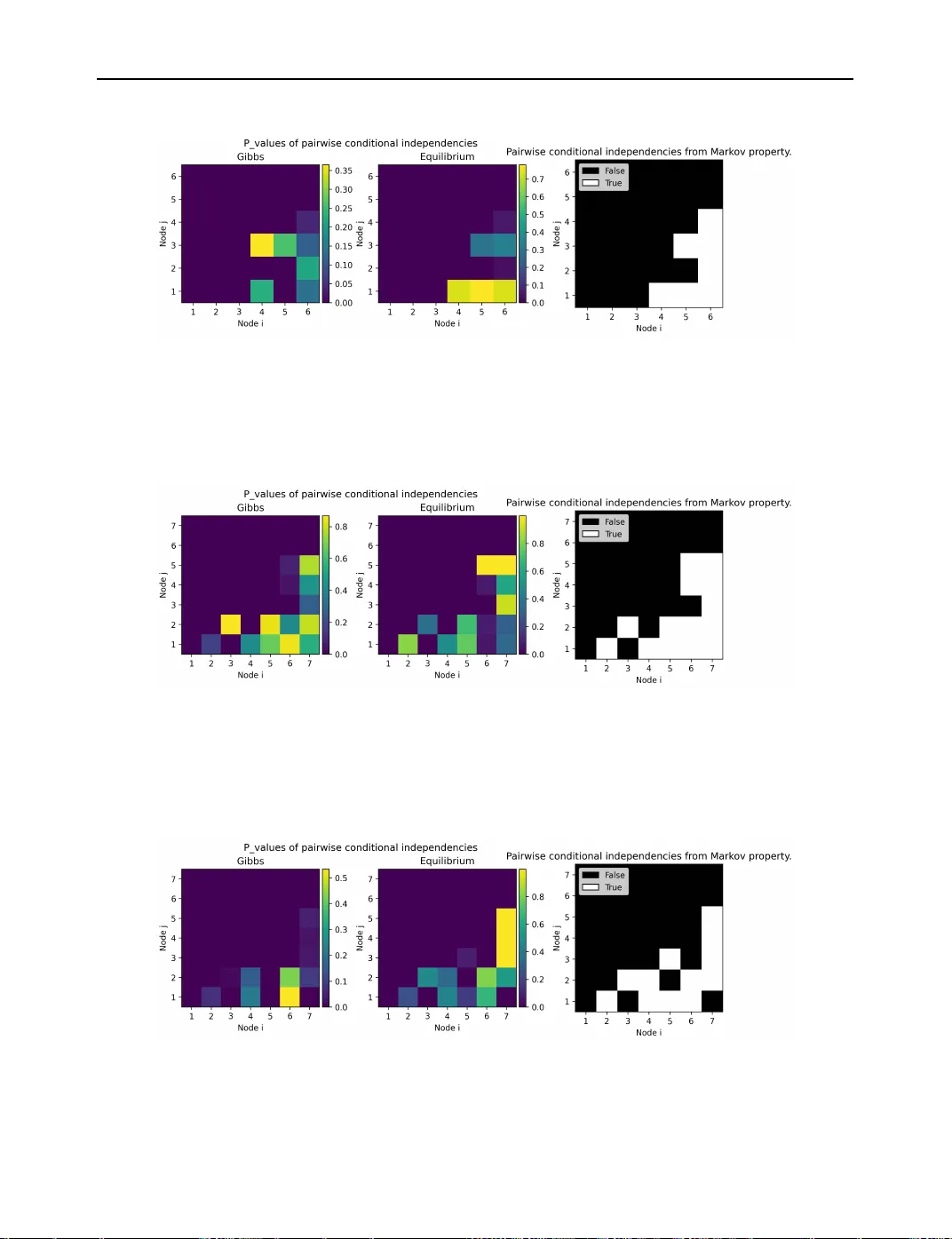
Interp retable Causal Graphical Mo dels fo r Equilib rium Systems with Confounding Kai Z. T eh, ∗ Ka yvan Sadeghi and T erry So o Depa rtment of Statistical Science, Universit y College London, Go wer Street, W C1E 6BT, London, UK ∗ Email for co rresp ondence. k ai.teh.21@ucl.ac.uk Abstract In applications, quantities of interest a re often mo delled in equilibrium or an equilibrium solution is sought. The p resence of confounding mak es causal inference in this setting challenging. We p rovide interpretable graphical mo dels for equilib rium systems with confounding using anterial graphs (Lauritzen and Sadeghi, 2018), a class of graphs containing directed acyclic graphs, ancestral graphs, and chain graphs. In this setting, w e provide valid graphical representations of b oth counterfactual va riables and observational va riables, which w e relate to counterfactual graphs (Shpitser and P earl, 2007) and single-wo rld intervention graphs (Richa rdson and Robins, 2013). As an application of this graphical representation, we p rovide an element-wise procedure of selecting adjustment sets that ﬂexibly include and exclude given covariates. Key wo rds: Causal Inference, Graphical Mo dels, Gibbs Sampler, Confounding 1. Introduction Causal inference aims to predict the consequences of in terven tions in the form of causal eﬀects. When interv entional data from randomised control trials are una v ailable, causal assumptions relating observ ational data to the interv ened setting are required to estimate causal eﬀects. A prominen t casual inference framework that captures these assumptions is the graphical mo del form ulation by Pearl (2009), based on directed acyclic graphs (DA Gs) in terpreted as structural causal mo dels (SCMs). Edges in a DA G are all directed and thus are not suitable in capturing symmetric relations b etw een v ariables such as relationships induced by equilibria and confounding. Ancestral graphs (Ric hardson and Spirtes, 2002) and chain graphs (F ryden b erg, 1990) ha ve been prop osed to represen t confounding (Richardson and Spirtes, 2002; Zhang, 2008) (see also Sadeghi and So o (2022)) or v ariables at equilibrium (Lauritzen and Richardson, 2002). An terial graphs (Lauritzen and Sadeghi, 2018) pro vide a natural generalisation of chain graphs, ancestral graphs, and D AGs, and also represent the marginalisation and conditioning of these classes of graphs (Sadeghi, 2016). In addition to directed edges, an terial graphs also con tain bidirected and undirected edges, whic h we will use to represent confounding and equilibrium relationships b etw een v ariables, resp ectively . W e will formalise these confounding and equilibrium relationships using a generalisation of SCMs. Our anterial graphical mo del th us enables causal inference for equilibrium systems with confounding, and uniﬁes and generalises causal graphical mo dels describ ed by Richardson and Spirtes (2002); Zhang (2008) and Lauritzen and Richardson (2002), for ancestral graphs and chain graphs, respectively . Causal inference using anterial graphs is also interpretable since causal notions such as in terven tions can b e expressed purely graphically as local mechanistic manipulations on the in tervened v ariables. T o demonstrate this in terpretability , in the same spirit as coun terfactual graphs (Shpitser and P earl, 2007) and single-w orld in terven tion graphs (Ric hardson and Robins, 2013), we will provide graphs that encode coun terfactual conditional indep endence assumptions b etw een observ ational v ariables and counterfactual v ariables in the case of anterial graphs. These counterfactual conditional indep endencies encode man y imp ortant assumptions for methods in causal inference. One such assumption is the conditional exchangabilit y assumption (Hernan and Robins, 1 2 T eh et al. 2020), which is imp ortant in tasks such as selecting an adjustment set of confounder cov ariates to control for confounding b etw een treatment and outcome v ariables. A v ariety of criteria hav e b een prop osed to select suc h a set of confounder co v ariates, such as the backdoor criterion of P earl (2009, Chapter 3.3.1) and the pre-treatment heuristics of Rubin (2009). Recen tly , there has also been work addressing other asp ects of suc h selection criteria, suc h as statistical eﬃciency (Rotnitzky and Smucler, 2020) and the limited structural knowledge of the underlying causal graph (Guo and Zhao, 2026). Based on marginalisation and conditioning operations developed for anterial graphs (Sadeghi, 2016), w e provide an element-wise algorithm to select an adjustment set constrained to include and exclude given co v ariates, which can arise in practice due to prohibitive costs or regulation requirements in areas suc h as clinical trials or algorithmic fairness. Our algorithm is prov ably correct under conditions such as when the counterfactual graphs provided is v alid. Compared to standard approac hes of selecting adjustmen t sets where the inclusion and exclusion constrain ts are enforced p ost-ho c, after eﬃciently enumerating all p ossible adjustment sets (v an der Zander et al., 2019), our approac h takes the constrain ts into accoun t directly in the algorithm. The structure of the pap er will b e as follows: Section 2 cov ers the relev ant bac kground, Section 3 cov ers the anterial graphical mo del of equilibrium systems with confounding, Section 4 cov ers interv entions and the extension of counterfactual graphs in this setting using our an terial graphical mo del, and Section 5 co vers the confounder selection algorithm. All pro ofs will b e deferred to the ﬁnal section. 2. Background 2.1. Probabilistic Graphs Let G denote a graph ov er a ﬁnite set of no des V ,with only one of the three types of edges: dir e cte d ( → ), undir e cte d ( — ), and bidire cte d ( ↔ ), connecting tw o adjacen t no des. Consider a sequence ⟨ i 0 , . . . , i n ⟩ of no des in the graph G . If every pair of consecutive no des is adjacent, then the sequence is a p ath ; if i 0 = i n , in addition, then the sequence is a cycle . If each edge b etw een consecutive adjacent no des i m and i m +1 is either undirected or directed as i m − → i m +1 , then the sequence is a semi-dir e cted p ath from i 0 to i n ; if in addition i 0 = i n and at least one of the edges is directed, then the sequence is a semi-dir e cte d cycle . In this work, we will consider anterial gr aphs (Lauritzen and Sadeghi, 2018). Deﬁnition 1 (An terial graphs) An anterial graph ov er a set of no des is a graph which may con tain directed, undirected, and bidirected edges that satisﬁes the following. 1. There do es not exist a semi-directed path b etw een tw o no des that are adjacent via a bidirected edge. 2. The graph do es not contain semi-directed cycles. By allowing only directed edges, we recov er the deﬁnition of a dir e cte d acyclic gr aph (DA G). Likewise excluding bidirected edges or no de conﬁgurations of the form i − k ↔ j (whic h is trivially satisﬁed by excluding undirected edges), we recov er the deﬁnition of chain graphs or ancestral graphs, resp ectively . F ollowing F rydenberg (1990), a chain c omp onent τ in an an terial graph G is a maximal set of no des suc h that every pair of no des x, y ∈ τ is connected by a sequence of undirected edges; thus all no des in G can be partitioned into chain components. Note that in the case of a D AG, each node is a c hain comp onent. Giv en a no de i ∈ V , let τ ( i ) denote the chain comp onent containing i . Given a set of no des C ⊆ V in a graph G , the neighb ors of C , denoted by ne( C ), are the set of no des x ∈ C such that x − i for some no de i ∈ C ; the p ar ents of C , denoted by pa( C ), are the set of no des x ∈ C such that x → i for some node i ∈ C ; the anterior of C , denoted by an t( C ), is the set of no des x ∈ C suc h that there exists a semi-directed path from x to some no de i ∈ C . Remark 1 When undir e cte d edges ar e absent, the anterior of C c oincides with the anc estors of C . Note that some authors let the neighb ors and anterior of the set C ⊆ V c ontain the set C itself, however, we do not. ♢ F or disjoin t subsets A, B , C ⊆ V , let A ⊥ G B | C denote the graphical separation of A and B given C in a graph G ; in the case of anterial graphs, this is understo o d as the separation criterion in Lauritzen and Sadeghi (2018, Section 3.2), which is simpliﬁed to the classical d-separation (P earl, 2009, Chapter 1.2.3) Causal Equilibrium Systems 3 when the graph G is a DA G, and m-separation for ancestral graphs; see also Lauritzen and Sadeghi (2018, Section 3.3). F or brevity , we will sometimes express the singleton set { i } ⊆ V , without the set braces, as i . The graphs G 1 and G 2 o ver the same no de set V are Markov equivalent if they induce the same graphical separations. In a DA G, each pair of non-adjacent no des are separated, say by their ancestors. How ever, an anterial graph need not b e maximal (see the graph G ∗ 0 in Figure 11 for example). Deﬁnition 2 (Maximal graphs) A graph G is maximal if for each pair of no des i and j in G , we hav e i not adjacent to j in G ⇒ i ⊥ G j | C for some C ⊆ V \{ i, j } . Lauritzen and Sadeghi (2018) characterised when an terial graphs are maximal. They also provided a graphical op eration max( · ) which maximises any given an terial graph G —returning a graph max( G ) with the follo wing prop erties. • The graph max( G ) is maximal. • The graphs max( G ) and G are Marko v equiv alent. • The graph G is a subgraph of max( G ). W e asso ciate a set of random v ariables X V = ( X 1 , . . . , X | V | ) with a joint distribution P to the set of no des V . W e will often write X ∼ P , if P is the law of X . Given a set A ⊆ V , let X A = ( X i ) i ∈ A , and A ⊥ ⊥ B | C denote the conditional indep endence of X A and X B giv en X C . If each graphical separation implies a corresp onding conditional indep endence, then we hav e the Markov pr op erty : Deﬁnition 3 (Marko v prop erty) A distribution P is Mark ovian to G if A ⊥ G B | C ⇒ A ⊥ ⊥ B | C for all disjoin t A, B , C ⊆ V . If w e hav e the reverse implication as well, then we hav e faithfulness . Deﬁnition 4 (F aithfulness) A distribution P is faithful to G if A ⊥ G B | C ⇐ ⇒ A ⊥ ⊥ B | C for all disjoint A, B , C ⊆ V . If the distribution P is faithful to some anterial graph G , then P is a comp ositional graphoid (Sadeghi, 2017, Theorem 17). Deﬁnition 5 (Comp ositional graphoid) A distribution P ov er V is a compositional graphoid if w e hav e the follo wing conditional indep endence prop erties. F or disjoint A, B , C , D ⊆ V , • (In tersection) A ⊥ ⊥ B | C ∪ D and A ⊥ ⊥ D | C ∪ B implies A ⊥ ⊥ B ∪ D | C , and • (Comp osition) A ⊥ ⊥ B | C and A ⊥ ⊥ D | C implies A ⊥ ⊥ B ∪ D | C . Remark 2 Examples of c ompositional gr aphoids ar e given by multivariate G aussian distributions. The assumption that a distribution is a c omp ositional gr aphoid is often made when attempting to faithful ly describ e a distribution via a gr aphic al mo del; se e Sade ghi (2017). ♢ Giv en a distribution P ov er v ariables X V , disjoint subsets M , C ⊆ V and x B , a ﬁxed v alue of X B , let P A ( · | x B ) denote the marginal of the conditional distribution P ( · | x B ) ov er X A (b y integrating out X V \ ( A ∪ B ) ). F or a distribution P V that is faithful to a DA G G , there does not necessarily exist a D AG to which the marginal distribution P V \ M is faithful. Lik ewise, there do es not necessarily exist a DA G to whic h the conditional distribution P ( · | x C ) is faithful. In the case where P is faithful to an anterial graph G , anterial graphs to which the marginal or conditional distributions are faithful alwa ys exist. An terial graphs are thus closed under marginalising and conditioning, unlike D AGs, chain graphs and ancestral graphs. Giv en an anterial graph G ov er the no des V and subset M ⊆ V , Sadeghi (2016) provides the graphical op eration α m to marginalise G , which 4 T eh et al. returns the anterial graph α m ( G ; M ) ov er no des V \ M such that for disjoint A, B , C ⊆ V \ M , we hav e A ⊥ G B | C ⇐ ⇒ A ⊥ α m ( G ; M ) B | C . (1) This corresp ondence captures the relationship b etw een the conditional indep endencies of a distribution P and its marginal distribution P V \ M . Similarly with conditioning, given any anterial graph G ov er the no des V and a subset C ⊆ V , Sadeghi (2016) provides the graphical op eration α c to condition G , which returns the anterial graph α c ( G ; C ) ov er no des V \ C such that for disjoint A, B , D ⊆ V \ C , we hav e A ⊥ G B | D ∪ C ⇐ ⇒ A ⊥ α c ( G ; C ) B | D . (2) This corresp ondence captures the relationship b etw een the conditional indep endencies of a distribution P and its conditional distribution P ( · | x C ). W e will be using these prop erties of marginalisation and conditioning to analyse the confounder selection algorithm prop osed in Section 5; see Theorem 5 for Algorithm 4. 2.2. Interventions and Confounder Selection A D AG G is often asso ciated to a structur al c ausal mo del with mutually indep enden t errors. Deﬁnition 6 (Structural causal mo del (SCM)) Let G b e a DA G where every no de i is asso ciated with a function f i and an error random v ariable ϵ i . An SCM consists of functional assignmen ts recursiv ely deﬁning observ ational random v ariables X V of the form X i = f i ( X pa( i ) , ϵ i ) , for every no de i ∈ V . W e let P be the law of X V , so that P is the observ ational distribution. When the errors are mutually indep enden t, the resulting joint distribution P is Marko vian to the DA G G (Pearl, 2009, Theorem 1.4.1); this result facilitates the use of graphical calculus on DA Gs to manipulate the SCM for the purp oses of causal inference, such as in the case of adjustment set selection. W e will prov e an analogue of this result when the distribution P is induced via SCMs of equilibriums with confounding; see Theorem 1. Using an SCM, interv ening on a treatment set C ⊆ V amounts to replacing the functional assignments of all X i where i ∈ C with some ﬁxed v alues a i , while keeping the functional assignments of all X j where j ∈ C ﬁxed. This replacemen t results in the deﬁnition of a diﬀerent set of interv ened random v ariables X do( a C ) V = ( X do( a C ) 1 , . . . , X do( a C ) | V | ), with which we asso ciate an interv entional distribution P do( a C ) . The new v ariables X do( a C ) V will b e referred to as in tervened v ariables in the scop e of this work. Note that X do( a C ) V are also known as p otential outcomes (Rubin, 1978, 2005). Let O ⊆ V denote the outcome set and X C the treatmen t v ariables. Expressing common causal estimands such as the c onditional aver age tr e atment eﬀe ct (CA TE) solely in terms of the observ ational distribution dep end on the following unc onfounde dness assumption: there exists an adjustment set S ⊆ V suc h that X do( a C ) O ⊥ ⊥ X C | X S (3) holds for all p ossible interv ened v alues a C . If there is no subset of S that satisﬁes (3), then S is minimal . The conditional indep endence (3) is also known as the conditional exchangabilit y condition (Hernan and Robins, 2020, Page 18). Graphically , this coupling has b een describ ed using approaches suc h as twin-net w orks (Balk e and Pearl, 1994), counterfactual graphs, (Shpitser and Pearl, 2007) and single-world interv en tion graphs (Richardson and Robins, 2013, 2023). These metho ds represent observ ational and interv ened v ariables in a single graph G ′ so that conditional indep endence relations b etw een observ ational and interv ened v ariables, such as (3), can b e expressed as classical d-separation in G ′ . Note that (3) requires that the joint distribution of the interv ened outcome v ariable X do( a C ) O and the observ ational v ariable X C to b e well-deﬁned; the required coupling b etw een observ ational and interv ened v ariables is sp eciﬁed by the shared errors ϵ V b et ween the SCM and the interv ened SCM. Causal Equilibrium Systems 5 In this w ork, w e will only b e concerned with the kind of coun terfactual assumptions that relate observ ational v ariables X V and interv ened v ariables X do( a C ) V where the interv ened v alue a C is ﬁxed, suc h as (3); relating interv ened v ariables X do( a C ) V and X do( a ′ C ) V for diﬀerent v alues a C and a ′ C is outside of our scop e. Thus, w e will consider only the set of treatment v ariables C and not the actual v alues a C of the interv en tion, and this will b e suppressed in our notation as X do( C ) V and P do( C ) . Note that such assumptions are still suﬃcient for expressing some of the causal estimands inv olving diﬀerent interv ened v alues such as the eﬀe ct of tr e atment on the tr e ate d (ETT). 2.3. Causal Interpretation of Chain Graphs Giv en a chain graph G , based on the factorisation prop erty of chain graphs (F rydenberg, 1990), Lauritzen and Richardson (2002) has proposed causal in terpretations of c hain graphs as a data generating pro cess ha ving tw o nested pro cesses. The outer pro cess expresses the relationship b etw een diﬀerent chain comp onen ts as X τ = f τ ( X pa( τ ) , ϵ τ ) (4) for some random error v ariable ϵ τ asso ciated to eac h chain comp onent τ , where the errors are jointly indep enden t. These can b e understoo d as SCM functional assignmen ts b y considering the chain comp onent as no des in a DA G. The inner pro cess then asso ciates each chain comp onent τ with a dynamical pro cess that has a conditional equilibrium distribution given x pa ( τ ). 3. Structured Equilibrium Models with Confounding W e will formally express the relationship betw een diﬀeren t c hain comp onents described in (4) with p otential confounding, as a structural equilibrium mo del. Deﬁnition 7 (Structural equilibrium mo del) Let τ 1 , . . . , τ n b e the parts of an ordered partition of V . Eac h part τ i is asso ciated with a function f τ i with arguments X pa( τ i ) , where pa( τ i ) ⊆ { τ 1 , . . . , τ i − 1 } , and an error random v ariable ϵ τ i . A structural equilibrium mo del consists of functional assignments of observ ational random v ariables X τ i of the following form X τ i = f τ i ( X pa( τ i ) , ϵ τ i ) . Note that the errors ϵ τ 1 , . . . ϵ τ n need not b e jointly indep endent. If all τ 1 , . . . , τ n are all singletons with join tly independent errors, then we recov er the deﬁnition of an SCM for D AGs—in this case, Lauritzen and Ric hardson (2002, Section 6.3) view Deﬁnition 7 as a data generating pro cess The notation pa( τ i ) suggests a corresp onding graph G . Indeed, given a structural equilibrium model, w e construct the corresp onding graph G b y considering, for each part τ ∈ { τ 1 , . . . , τ n } , how τ is connected to pa( τ ) based on the functional assignment of τ . This construction is formalised as Algorithm 1. Algorithm 1 The corresp onding graph G of a structural equilibrium mo del Input: Structural equilibrium mo del Output: Graph G . F or every part τ ∈ { τ 1 , . . . , τ n } , let J τ ( · | x pa( τ ) ) b e the law of f τ ( x pa( τ ) , ϵ τ ). 1: F or no des i and j in τ , if i   ⊥ ⊥ j | τ \{ i, j } holds for J τ ( · | x pa( τ ) ), then add undirected edge i − j . 2: F or no des i ∈ pa( τ ) and j ∈ τ , if for all v alues of x ( τ ∪ pa( τ )) \{ i,j } , the conditional marginal J τ i ( · | x τ \ i ; x pa( τ ) ) dep ends on the v alue of x i , then add the directed edge i → j . 3: F or parts τ and τ ′ , if ϵ τ   ⊥ ⊥ ϵ τ ′ , then add bidirected edges i ↔ j for every no de i ∈ τ and j ∈ τ ′ . F or examples of structural equilibrium mo dels and their corresp onding graphs, see Figures 4, 5, and 6 in Section 3.2. 6 T eh et al. Remark 3 Step 1 of Algorithm 1 ensur es that J τ ( · | x pa( τ ) ) satisﬁes the p airwise Markov pr op erty with r esp e ct to (w.r.t.) to the c onstructe d undir e cte d graph over nodes in τ and that no sub graph of the undir e cte d gr aph satisﬁes this prop erty. The c ondition in Step 2 of Algorithm 1 c an b e suc cinctly expr esse d as i   ⊥ ⊥ j | τ ∪ pa( τ ) \{ i, j } using the formulation in Constantinou and Dawid (2017, The or em 3.5), which al lows the expr ession of dep endence on ﬁxe d p ar ameters x pa( τ ) as an extende d c onditional indep endenc e statement. These (extende d) c onditional indep endencies over τ and pa( τ ) ar e r epr esente d gr aphic al ly using Algorithm 1. Se e Figur e 1. ♢ τ ∪ pa( τ ) pa(3) ∪ ne(3) 1 3 4 5 2 Fig. 1: Chain comp onent τ = { 3 , 4 , 5 } and parents pa( τ ) = { 1 , 2 } . F or every no de i ∈ τ , Algorithm 1 constructs ne( i ) and pa( i ) such that the conditional marginal J τ i ( · | x τ \ i ; x pa( τ ) ) do es not dep end on no des outside of pa( i ) ∪ ne( i ) (formalised as Lemma 10 in the Pro ofs Section). F or every part τ , Step 1 of Algorithm 1 constructs the chain comp onents of the graph G using the distribution J τ ( · | x pa( τ ) ) of f τ ( x pa( τ ) , ϵ τ ) from the mo del. F or every no de i ∈ τ , step 2 of Algorithm 1 then uses the i -marginal of the conditional distribution J τ i ( · | x ne( i ) ; x pa( τ ) ) to determine the parents of i for the constructed G . Step 3 of the algorithm then includes bidirected edges in the constructed graph G to represen t dep enden t noises of the mo del. Remark 4 (Relating parts to chain comp onents of G ) Consider the p art τ that de c omp oses in multiple c onne cte d c omp onents τ ′ 1 , . . . , τ ′ m after p erforming Step 1 of Algorithm 1. These c onne cte d c omponents ar e the chain c omp onents of the corr esp onding gr aph G . Sinc e Step 1 of Algorithm 1 c onstructs an undir e cte d gr aph of chain c omponents such that J τ ( · | x pa( τ ) ) satisﬁes the p airwise Markov pr operty, if J τ ( · | x pa( τ ) ) satisﬁes the interse ction pr operty, then it c an b e se en that the chain c omp onents ar e jointly independent using the glob al Markov pr op erty, sinc e the chain c omp onents ar e not c onnecte d by p aths. Thus, the functional assignment X τ = f τ ( X pa( τ ) ,ϵ τ ) for the p art τ c an b e de c omp ose d into multiple functional assignments: X τ ′ i = f τ ′ i ( X pa( τ ) , ϵ τ ′ i ) , wher e τ ′ i ∈ { τ ′ 1 , . . . , τ ′ m } , with ϵ τ = ( ϵ τ ′ 1 , . . . , ϵ τ ′ n ) , wher e the c onstituent errors are jointly indep endent. Having multiple chain c omp onents fr om a p art do es not aﬀe ct the pr o of of The or em 1. However, without loss of generality, we wil l c onsider structur al e quilibrium mo dels such that, for e ach p art, τ do es not de c omp ose w.r.t. the distribution J τ ( · | x pa( τ ) ) . Thus we wil l assume that e ach p art τ is a chain c omp onent in the c orr esp onding gr aph G . ♢ If the corresponding graph G is anterial, then the distribution P , assumed to b e a comp ositional graphoid, induced from the structural equilibrium mo del is Marko vian to G . Theorem 1 (Mark ov prop erty for structural equilibrium mo dels) L et P b e the joint distribution over the variables X V induc e d fr om a structur al e quilibrium mo del and let the c orr esp onding gr aph G over the no des V , as c onstructe d in Algorithm 1, b e anterial. If P is a c omp ositional graphoid, then P is Markovian to G . Throughout this work, we will assume structural equilibrium mo dels that correspond to an terial graphs, via Algorithm 1. In addition to Deﬁnition 7, these mo dels hav e an additional constraint: for any parts Causal Equilibrium Systems 7 τ ′ 1 , τ ′ m ∈ { τ 1 , . . . , τ n } , if there is a sequence of parts ⟨ τ ′ 1 , τ ′ 2 , . . . , τ ′ m − 1 , τ ′ m ⟩ such that τ ′ i in tersects pa( τ ′ i +1 ) for each consecutive parts τ ′ i and τ ′ i +1 , then ϵ τ ′ 1 ⊥ ⊥ ϵ τ ′ m . Indeed, this condition can b e graphically expressed as the lack of semi-directed paths b etw een endp oints of a bidirected edge. See Section A.5 on why the an terial assumption is imp ortan t for causal interpretabilit y . In the case where the corresp onding graph is a c hain graph, Lauritzen and Richardson (2002, Proposition 6) giv es the Mark ov property for G when viewing the c hain graph as a D AG with chain comp onents as no des. Theorem 1 enables the consideration of conditional indep endencies inv olving every subset of no des, addressing the remark from Dawid (2009) regarding the full extraction of conditional indep endencies from the c hain graph. When the parts of the structural equilibrium mo del are singletons, Algorithm 1 returns a graph of only directed and bidirected edges. When the errors in the structural equilibrium model are join tly independent, Algorithm 1 returns a chain graph. With the additional assumption that the induced distribution is a compositional graphoid, Theorem 1 extends the Marko v property results in Sadeghi and Soo (2022, Theorem 27) for ancestral graphs and Lauritzen and Richardson (2002) for chain graphs. Step 3 of Algorithm 1 connects either all or none of the no des b etw een the chain comp onents τ and τ ′ with bidirected edges. Deﬁnition 8 (Chain-connected graph) A graph G is chain-c onne cte d if for all no des i and j , we hav e i ↔ j ⇒ i ↔ k for all k ∈ τ ( j ) . Th us, it can b e seen that the corresp onding graph G is chain-connected. This can b e interpreted as all no des in the chain comp onent τ sharing the same error ϵ τ . Throughout this work, we will describe structural equilibrium mo dels using chain-connected anterial graphs. Common graph classes such as DA Gs, ancestral graphs and chain graphs are still a sub class of chain-connected anterial graphs. Remark 5 In principle, Step 3 of Algorithm 1 c an b e mo diﬁe d to add bidir e cte d e dges b ase d on c onditional indep endencies of the induc e d joint distribution P , while stil l pr eserving the Markov pr op erty r e quir e d. However, this appr o ach is inste ad distributional, dep ending on the actual c oupling of the err ors, and no longer pur ely structur al. dep ending only on the independencies of the err ors, which al lows for c ausal op er ations in an interpr etable graphic al manner. Se e also a similar ar gument on the imp ortanc e of the anterial assumption on c ausal interpr etability in Se ction A.5. ♢ 3.1. Interp reting the constructed graphical mo del G In Lauritzen and Richardson (2002), each chain comp onent τ of a chain graph mo del is asso ciated with a dynamical pro cess, such as a Gibbs sampler (Geman and Geman, 1984), having a conditional equilibrium distribution given x pa( τ ) , whic h we denote as J τ ( · | x pa( τ ) ). As suggested b y the notation, given a structural equilibrium mo del, for every part τ , we will similarly asso ciate the la w J τ ( · | x pa( τ ) ) of f τ ( x pa( τ ) , ϵ τ ) with the equilibrium distribution of the Gibbs sampler as follows. Lab el the no des in the chain comp onent from 1 to | τ | . Let X 0 τ = x 0 τ b e some initial v alues and m 0 = 1 b e the starting no de of the Gibbs sampler, at every timestep t the v alues X t τ and no de m t are up dated as follo ws: m t = m t − 1 + 1 mo d | τ | , X t τ \ m t = x t − 1 τ \ m t , and X t m t ∼ J τ m t ( · | x t − 1 ne( m t ) ; x pa( m t ) ) . (5) Remark 6 Given a structur al e quilibrium mo del, interpr eting J τ ( · | x p a ( τ ) ) as the equilibrium distribution of some dynamical pr o c ess is only re quir e d to deﬁne sensible notions of interventions in Se ction 4. Observational ly, it suﬃc es to c onsider J τ ( · | x p a ( τ ) ) only, sinc e The or em 1 is a statement on the observational joint distribution and ther efor e holds r e gar d less of the exact dynamic al pro c ess. ♢ 8 T eh et al. Despite anterial graphs b eing closed under marginalisation and conditioning, we will discuss wh y in terpretations based on marginalisation and conditioning of existing graph classes are not suitable for c hain-connected anterial graphs. Marginalising chain graphs results in anterial graphs (Sadeghi, 2016). Building on top of existing chain graph interpretations (Lauritzen and Richardson, 2002), one may b e tempted to consider anterial graphs as the marginal of a chain graph with latent v ariables, with bidirected edges i ↔ j representing a laten t v ariable b etw een no des i and j . How ever, Example 1 shows the problem with such an interpretation. G 4 2 3 1 G ′ 4 2 U 1 U 2 3 1 α m ( G ′ ; { U 1 , U 2 } ) 4 2 3 1 Fig. 2: Left: Chain-connected anterial graph G . Middle: Interpretation of bidirected edges 3 ↔ 4 and 2 ↔ 4 in G as unobserved latent v ariables U 1 and U 2 resp ectiv ely , from the chain graph G ′ . Right: Graph α m ( G ′ ; { U 1 , U 2 } ) obtained by marginalising G ′ o ver the latent v ariables U 1 and U 2 . Example 1 (Problem with interpretations based on marginalisation) Consider Figur e 2 and interpr et the bidir e cte d e dges in the chain-c onne cte d anterial gr aph G as the existenc e of unobserve d latent variables U 1 and U 2 , as shown in the chain gr aph G ′ . Mar ginalising over U 1 and U 2 in G ′ r esults in α m ( G ′ ; { U 1 , U 2 } ) which is not Markov e quivalent to G ; inde e d, 1 ⊥ G 2 | 3 , but this sep ar ation do es not hold in the mar ginalisation α m ( G ′ ; { U 1 , U 2 } ) . Similar issues with marginal chain graph mo dels hav e b een raised by Shpitser (2015) and were resolved using graphs con taining undirected, directed, and bidirected edges. How ever, the directed edges in suc h graphs do not seem to hav e a clear interpretation (Shpitser, 2015, Section 2). Similarly , conditioning ancestral graphs results in anterial graphs (Sadeghi, 2016). Building on top of existing interpretations of ancestral graphs (Richardson and Spirtes, 2002; Sadeghi and So o, 2022), it may also b e tempting to interpret an terial graphs as the conditional of ancestral graphs with selection v ariables, where the undirected edges i − j is in terpreted as conditioning on a selection bias v ariable betw een the nodes i and j from an ancestral graph. How ever, Example 2 shows a similar problem with such an interpretation. G 4 2 3 1 G ′ 4 2 3 1 L 1 α c ( G ′ ; L 1 ) 4 2 3 1 Fig. 3: Left: Chain-connected anterial graph G . Middle: Interpretation of the undirected edge 2 − 3 as the selection bias v ariable L 1 from the ancestral graph G ′ . Right: Graph α c ( G ′ ; L 1 ) obtained by conditioning G ′ o ver the selection bias v ariable L 1 . Causal Equilibrium Systems 9 Example 2 (Problem with interpretations based on conditioning) Consider Figur e 3 and interpr et the undir e cte d e dge 2 − 3 in the chain-conne cte d anterial gr aph G as the existenc e of sele ction variables L 1 , as shown in the anc estr al gr aph G ′ . Conditioning on L 1 in G ′ r esults in α c ( G ′ ; L 1 ) , which is not Markov e quivalent to G ; indee d, 1 ⊥ G 4 but this sep aration does not hold in the c onditional gr aph α c ( G ′ ; L 1 ) . 3.2. Examples and simulations T o illustrate Theorem 1, we will simulate data from structural equilibrium mo dels that corresp ond to the c hain-connected anterial graphs in Figures 4, 5, and 6 in Python. Since the joint distribution in Theorem 1 is induced from the distributions ov er chain comp onents J τ ( · | x pa( τ ) ), which we interpret as equilibrium of Gibbs samplers in (5), the simulation also allows us to test the v alidit y of the Marko v prop erty of the structural equilibrium mo del when interpreted as Gibbs samplers in ﬁnite-time. G 1 2 4 3 5 6 1 X 1 = ϵ 1  X 2 X 3  =  1 3  X 1 +  ϵ 2 ϵ 3  X 4 = ϵ 4  X 5 X 6  =  1 1 1 1  X 2 X 4  +  ϵ 5 ϵ 6  ϵ 1 ∼ N (0 , 1)  ϵ 2 ϵ 3  ∼ N  0 ,  1 2 2 5  ϵ 4 = ϵ 2 + ϵ 3 + ε, ε ∼ N (0 , 1)  ϵ 5 ϵ 6  ∼ N  0 ,  1 1 1 2  Fig. 4: Left: Corresponding chain-connected an terial graph G 1 . Middle: Structural equilibrium model. Conditioning on 5, the distribution J { 5 , 6 } 6 ( · | x 5 ; x { 2 , 4 } ) do es not dep end on x { 2 , 4 } , thus pa(6) = ∅ . Right: Distribution and coupling of the error v ariables. W e will consider the structural equilibrium model which corresp onds to the graph G 1 in Figure 4. W e sample 10000 data p oints directly from the structural equilibrium model (using the equilibrium distributions) and 1000 data points using a Gibbs sampler of the conditional normal distributions J { 2 , 3 } ( · | x 1 ) and J { 5 , 6 } ( · | x 2 , x 4 ) with a burn-in of 10000 steps. Using b oth sampled datasets, we p erform a Fisher-Z test (using the causal-learn (Zheng et al., 2024) pack age) with a null hypothesis of pairwise conditional indep endence of the form i ⊥ ⊥ j | ant( i, j ) for ev ery pair of no des i and j . The Marko v prop ert y w.r.t. the graph G 1 w ould imply pairwise conditional indep endencies for some no des i and j . The p-v alues for every pair of no des are shown in Figure 17 in Section A.7. Next, w e consider the structural equilibrium mo del which corresp onds to the graph G 2 in Figure 5. Again, the p-v alues for the pairwise conditional indep endence tests are shown in Figure 18 in Section A.7. W e will use the structural equilibrium mo del which corresp onds to the graph G 3 in Figure 6. The p-v alues for the pairwise indep endence tests are shown in Figure 19 in the Section A.7. In Figure 19, high p-v alues indicate insuﬃcien t evidence for rejecting the null hypothesis in fav our of the alternativ e h yp othesis where i   ⊥ ⊥ j | ant( i, j ), implying conditional independence. W e see that the Fisher Z-test rejects the null hypothesis in a manner consisten t with the conditional indep endencies implied by the Marko v property of Theorem 1. Note that due to the higher dimensionality when sampling { 3 , 4 , 5 } , the p-v alues of the pairwise conditional indep endencies 5 ⊥ ⊥ 1 | { 2 , 3 , 4 } and 5 ⊥ ⊥ 3 | { 2 , 1 , 4 } are on the order of ab out 10 − 7 , while all the other returned p-v alues are close to 0. 4. Graphical Interventions of Structural Equilib rium Models Giv en a structural equilibrium mo del with the corresp onding graph G , using the interpretation of a chain comp onen t τ of G as the Gibbs sampler in (5), an interv ention on a treatment set C ⊆ V (to interv ened v alues a C ) can b e expressed through the following interv ened Gibbs sampler by replacing the up dating of 10 T eh et al. G 2 3 4 5 6 7 1 2 X 1 = ϵ 1 X 2 = ϵ 1  X 3 X 4  =  − 2 / 3 1 1 / 3 − 2  X 1 X 2  +  ϵ 3 ϵ 4  X 5 = ϵ 5  X 6 X 7  =  1 2  X 3 +  ϵ 6 ϵ 7  ϵ 1 ∼ N (0 , 1) ϵ 2 ∼ N (0 , 1)  ϵ 3 ϵ 4  ∼ N  0 ,  2 / 3 1 / 3 1 / 3 2 / 3  ϵ 5 = ϵ 3 + ϵ 4  ϵ 6 ϵ 7  ∼ N  0 ,  1 2 2 5  Fig. 5: Left: Corresponding chain-connected an terial graph G 2 . Middle: Structural equilibrium model. Conditioning on 3, the distribution J { 3 , 4 } 4 ( · | x 3 ; x { 1 , 2 } ) dep ends on x 2 only , thus pa(4) = 2, similarly we ha ve pa(3) = 1. Right: Distribution and coupling of the error v ariables. G 3 3 4 6 5 7 1 2 X 1 = ϵ 1 X 2 = ϵ 2 X 3 X 4 X 5 ! = − 11 / 12 − 1 / 4 5 / 6 1 / 2 − 1 / 4 − 1 / 4 !  X 1 X 2  + ϵ 3 ϵ 4 ϵ 5 ! X 6 = ϵ 6 X 7 = X 6 + ϵ 7 ϵ 1 ∼ N (0 , 1) ϵ 2 ∼ N (0 , 1) ϵ 3 ϵ 4 ϵ 5 ! ∼ N 0 , 11 / 12 − 5 / 6 1 / 4 − 5 / 6 5 / 3 − 1 / 2 1 / 4 − 1 / 2 1 / 4 !! ϵ 6 = ϵ 3 + ϵ 4 + ϵ 5 ϵ 7 = ϵ 1 + ε, ε ∼ N (0 , 1) Fig. 6: Left: Corresp onding Chain-connected anterial graph G 1 . Middle: Structural equilibrium mo del. 3 ⊥ ⊥ 5 holds for the distribution J { 3 , 4 , 5 } ( · | x { 2 , 4 } ), thus 3 is not connected to 5. Conditioning on ne(4), the distribution J { 3 , 4 , 5 } 4 ( · | x { 3 , 5 } ; x { 1 , 2 } ) do es not dep end on x { 1 , 2 } , th us pa(4) = ∅ . Likewise for pa(3) = 1 and pa(5) = 2. Right: Distribution and coupling of the error v ariables. the treatmen t no des in C with ﬁxed assignments. This replacemen t results in the intervene d Gibbs sampler as follo ws, expressed using the notation of the Gibbs sampler in (5): m t = m t − 1 + 1 mo d | τ | , if m t ∈ C, X t τ \ C = x t − 1 τ \ C , and X t τ ∩ C = a τ ∩ C , if m t ∈ C, X t τ \ m t = x t − 1 τ \ m t , and X t m t ∼ J τ m t ( · | x t − 1 ne( m t ) ; x pa( m t ) ) , (6) with the conditional distribution J τ m t ( · | x t − 1 ne( m t ) ; x pa( m t ) ) b eing the same in the Gibbs sampler (5) of the structural eq uilibrium mo del. Causal Equilibrium Systems 11 The resulting equilibrium distribution J τ , do( C ) ( · | x pa( τ ) ) on the chain comp onent τ is J τ , do( C ) ( · | x pa( τ ) ) = J τ τ \ C ( · | a τ ∩ C ; x pa( τ ) ) δ τ ∩ C ( a τ ∩ C ) , (7) where J τ τ \ C ( · | a τ ∩ C ; x pa( τ ) ) is the conditional distribution of the equilibrium distribution J τ ( · | x pa( τ ) ) of the pre-interv ened Gibbs sampler (5) and δ τ ∩ C ( a τ ∩ C ) is the delta function that tak es the v alue 1 when X τ ∩ C tak es the interv ened v alues a τ ∩ C ; this is a lo cal version of Lauritzen and Richardson (2002, Section 6.4, Equation 18). F rom the distributions J τ , do( C ) ( · | x pa( τ ) ), we deﬁne the resulting intervene d structur al e quilibrium mo del by replacing the assignments for all c hain components τ such that τ ∩ C  = ∅ in the structural equilibrium mo del with X τ = f do( C ) τ ( X pa( τ ) , ϵ τ ) , (8) suc h that • f do( C ) τ ( x pa( τ ) , ϵ τ ) ∼ J τ , do( C ) ( · | x pa( τ ) ), and • the chain comp onent errors ϵ τ 1 , . . . , ϵ τ n ha ve the same joint distribution as the errors in the observ ational structural equilibrium mo del (pre-interv en tion). The interv ened structural equilibrium mo del induces a new set of interv ened random v ariables X do( C ) V with whic h we asso ciate a joint interv entional distribution P do( C ) . Remark 7 Gener al ly, in structur al e quilibrium mo dels, the joint interventional distribution is not e quivalent to the joint c onditional distribution. However, this equivalenc e holds for the c onditional distribution of the variable given its p arents. This e quivalenc e is c omp atible with the r elationship in (7) . ♢ Remark 8 L auritzen and Richar dson (2002) also c onsider L angevin diﬀusions in lieu of Gibbs samplers. Given an observational distribution P , the interventional distribution P do( c ) obtaine d from an intervene d dynamic al pr o c ess using (8) dep ends on the dynamic al pr o c ess b eing c onsider e d. A Gibbs sampler is chosen for this work as the dynamic al pr o c ess, sinc e the r esulting intervention c an b e expr esse d purely gr aphic al ly (see Algorithm 2); the same c annot b e said ab out other dynamic al pr o c esses in L auritzen and Richar dson (2002) such as L angevin diﬀusions, for which the notion of intervention deﬁne d wil l dep end on diﬀusion p ar ameters. Note that without assuming the dynamic al pr o c ess to b e a Gibbs sampler, an e quilibrium distribution may not exist after intervening the dynamic al pr o c ess. ♢ 4.1. Rep resenting interventions graphically Via a graphical op eration (Algorithm 2) on the corresponding graph G of the observational structural equilibrium mo del, we can describ e the interv entional distribution P do( C ) after interv ening on a treatment set C . Algorithm 2 Interv ening chain-connected anterial graphs Input: chain-connected anterial graph G , no de subset C ⊆ V Output: chain-connected anterial graph do C ( G ) F or all i ∈ C , 1: for no des j such that i − j , if j ∈ C , then replace with i → j ; if j ∈ C , then remov e edge i − j , 2: remov e all directed edges into i , and 3: remov e all bidirected edges i ↔ j . Algorithm 2 ﬁrst mo diﬁes undirected edges of no des in the treatment set C and then remov es directed and bidirected edges connected to C . See Figure 7 for an illustration of Algorithm 2. When G is a D AG, only Step 2 of Algorithm 2 is performed, and Algorithm 2 reduces to a standard graphical interv ention for DA Gs. Since in terven tions can b e expressed distributionally as a truncated 12 T eh et al. G , C = { 2 , 3 } 6 2 3 1 4 5 6 2 3 1 4 5 do { 2 , 3 } G Fig. 7: Left: Input chain-connected anterial graph G and treatment set C = { 2 , 3 } . Right: Output do C ( G ) after remo ving bidirected and directed edges in to C . factorisation of the observ ational distribution, the interv en tional distribution is Marko vian to do C ( G ) (Spirtes et al., 2000, Theorem 3.6). Theorem 2 similarly describ es P do( C ) from structural equilibrium mo dels using the in tervened (an terial) graph do C ( G ). Theorem 2 (Marko v prop erty for in terv en tions) L et P do( C ) b e the interventional distribution (fr om intervening on a tr e atment set C ) induc e d fr om a structural equilibrium mo del c orr esp onding to the chain-c onne cte d anterial graph G . If P do( C ) is a c omp ositional gr aphoid, then P do( C ) is Markovian to do C ( G ) . Note that the interv ened structural equilibrium mo del is still a structural equilibrium mo del. Using the relationship in (7), Algorithm 2 constructs the corresp onding graph do C ( G ) from the observ ational graph G . Theorem 1 is used to show Theorem 2. Remark 9 (The splitting of chain comp onents when interv ening can b e dealt with similarly as in Remark 4.) In Figur e 7, the chain c omp onent { 2 , 3 , 4 , 5 } in G is split into multiple chain c omp onents in do C ( G ) . In gener al, given a chain c omp onent τ in G , the nodes in τ \ C c an b e p artitione d into diﬀer ent chain c omp onents τ do i in do C ( G ) , such that S n i =1 τ do i = τ \ C . As ar gue d in R emark 4 (by the glob al Markov pr op erty of the c onstructe d τ ), these c omp onents τ do i ar e jointly indep endent given a τ ∩ C , then we can de c omp ose the functional assignment X τ = f do ( C ) τ ( X p a ( τ ) , ϵ τ ) in (8) into X τ ∩ C = a τ ∩ C , and X τ do i = f τ do i ( X pa( τ ) , X τ ∩ C , ϵ τ do i ) , for e ach τ do i ∈ { τ do 1 , . . . , τ do n } , such that ϵ τ = ( ϵ τ do 1 , . . . , ϵ τ do n ) wher e e ach ϵ τ do i ar e jointly indep endent and f τ do i ( x pa( τ ) , x τ ∩ C , ϵ τ do i ) ∼ J τ τ do i ( · | a τ ∩ C ; x p a ( τ ) ) . ♢ 4.2. Counterfactual Interpretations In line with counterfactual interpretations in (P earl, 2009, Chapter 7); Balke and Pearl (1994), after in tervening on a treatment set C , using the structural equilibrium mo del, a coupling betw een observ ational v ariables X V and in tervened v ariables X do( C ) V is induced via common errors. Here, we describ e this coupling, and provide a graphical representation of this coupling. Consider a structural equilibrium mo del with the corresp onding c hain-connected anterial graph G . Given some chain comp onent τ in G , interv ention on a treatment set C ⊆ V by setting X C = a C for some ﬁxed v alue a C induces a coupling b etw een observ ational v ariables X τ and interv ened v ariables X do( C ) τ via the common error ϵ τ of the functional assignmen ts of the com bined structural equilibrium model, shown as follo ws: Causal Equilibrium Systems 13 X τ = f τ ( X pa( τ ) , ϵ τ ) , and X do( C ) τ = f do( C ) τ ( X do( C ) pa( τ ) , ϵ τ ) , if τ ∩ C  = ∅ X do( C ) τ = f τ ( X do( C ) pa( τ ) , ϵ τ ) , if τ ∩ C = ∅ , (9) where f do( C ) τ is the interv ened function from (8). 4.2.1. Representing the coupling graphically Giv en an anterial graph G , and a no de subset C ⊆ V , we apply the graphical op eration introduced in Algorithm 3, and denote the resulting graph as ϕ ( G ; C ). See Figure 8 for an illustration of Algorithm 3. Algorithm 3 Counterfactual Graph, ϕ Input: anterial graph G , no de subset C ⊆ V Output: graph ϕ ( G ; C ) 1: Repro duce G and construct do C ( G ), relab elling all the no des i in do C ( G ) as i do( C ) . 2: F or no des i ∈ C in G such that C ∩ ant(i) = ∅ , remov e i do( C ) and replace edges b et ween i do( C ) and no des of the form j do( C ) with the same edge b etw een i and j do( C ) . 3: Add bidirected edges based on T able 1. If in G Then 1. i ∈ C add i do( C ) ↔ i 2. i ↔ j and i ∈ C add i do( C ) ↔ j 3. j ∈ τ ( i ) and i ∈ C add i do( C ) ↔ j T able 1. Bidirected edges b etw een relab elled no des in do C ( G ) and no des in G , based on conditions on the corresponding nodes in G . G 2 1 C 5 3 6 4 do C ( G ) 2 do( C ) 1 do( C ) 5 do( C ) 3 do( C ) 6 do( C ) 4 do( C ) 2 1 5 3 6 4 2 do( C ) 5 do( C ) 3 do( C ) 6 do( C ) ϕ ( G ; C ) 2 1 5 3 6 4 2 do( C ) 5 do( C ) 3 do( C ) 6 do( C ) Fig. 8: Consider the input an terial graph G with C = 2. Left: Algorithm 3 ﬁrst creates do C ( G ) using Algorithm 2 with the no des relabelled alongside input graph G . Middle: Algorithm 3 merges nodes in G and do C ( G ). Right: Algorithm 3 then introduces bidirected edges b etw een G and do C ( G ) based on T able 1 to obtain ϕ ( G ; 2). Algorithm 3 ﬁrst introduces all the interv ened v ariables X do( C ) alongside the observ ational v ariables X V . F or a no de i in G such that there does not exist a semi-directed path in G from treatment set C to no de i , the observ ational v ariable X i is equal to X do( C ) i . Step 2 of Algorithm 3 accounts for this equality b y merging all such observ ational v ariables X i and interv ened v ariables X do( C ) i , represented b y the no des i 14 T eh et al. and i do( C ) , resp ectively , into the node i . The edges betw een i do( C ) and the other no des j do( C ) are preserv ed as the same edge b etw een i and j do( C ) . T able 1 introduces bidirected edges b etw een no des i do( C ) and no des j in G to capture the dep endence of the chain comp onent errors ϵ τ ( i ) and ϵ τ ( j ) that are shared b etw een the corresp onding v ariables X do( C ) τ ( i ) and X j (since errors are shared in (9)), when the corresp onding no de i in G is not in treatment set C . In the case of D AGs, Algorithm 3 reduces to the construction of coun terfactual graphs from Shpitser and P earl (2007), where the common errors are marginalised ov er. Using the structural equilibrium mo del (corresp onding to graph G ), the coupling b etw een observ ational and in tervened v ariables is describ ed via ϕ ( G ; C ). Let no de i do( C ) in graph ϕ ( G ; C ) represent X do( C ) i . Theorem 3 (Marko v property of the coun terfactual in terpretation) L et the observational r andom variables X V b e induc e d fr om a structur al e quilibrium mo del c orr esp onding to the chain-conne cte d anterial gr aph G . L et the c ombined structur al e quilibrium mo del in (9) induc e the joint distribution P ∗ b e the joint distribution over X V and X do( C ) V . If P ∗ is a c omp ositional gr aphoid, then P ∗ is Markovian to ϕ ( G ; C ) . Theorem 3 is shown by observing that the combined structural equilibrium mo del (9) is another structural equilibrium mo del, with the corresp onding graph ϕ ( G ; C ). Theorem 1 is used to show Theorem 3. Note that the no des merged in Step 2 of Algorithm 3 correspond to coun terfactual v ariables that are equiv alent to observ ational v ariables, that is, X do( C ) i = X i ; thus Theorem 3 describ es the full joint distribution of observ ational and interv ened v ariables. This merging step also av oids certain deterministic relationships betw een no des in the graph ϕ ( G ; C ), which can lead to violations of the faithfulness condition, leading to erroneous results as highlighted in Richardson and Robins (2013, Figure 15). How ever, errors are still shared b etw een observ ational and interv ened v aribles, as indicated by the bidirected edge 3 ↔ 3 do( C ) in ϕ ( G ; C ) of Figure 8, whic h can potentially lead to violations of faithfulness. This motiv ates an alternativ e graphical representation inspired b y single-w orld in terven tion graphs (SWIGs) from Ric hardson and Robins (2013). 4.2.2. Single-world interpretation Using Algorithm 3, the constructed ϕ ( G ; C ) describes the relationship of b oth observ ational and in terven tional ve rsions of the same v ariable en tailed by the combined structural equilibrium mo del (9), represen ted by having b oth i do( C ) and i as no des in the same graph. Ho wev er, outside of settings where one has a full description of the underlying data generating pro cess (in our case, the structural equilibrium mo del), causal inference has the fundamental problem where only one v ersion of the same v ariable is observed (Holland, 1986). T o accommodate this issue, we will also graphically represen t the single-world counterfactual distribution consisting of only one v ersion (observ ational or in tervened) of eac h v ariable that is not in the treatment set C , in line with Richardson and Robins (2013). Let the posterior of C in the observ ational graph G be given by p o( C ) = { j ∈ C : there is a semi-directed path from i ∈ C to j in G } . By marginalising the coun terfactual graph ϕ ( G ; C ) using α m with M = p o( C ), w e obtain α m ( ϕ ( G ; C ); p o( C )), which we call ϕ ′ ( G ; C ); see Figure 9 for an example. Based on Theorem 3, we hav e the following. Prop osition 4 (Mark ov property of the single-w orld in terpretation) L et the c ombined structur al e quilibrium mo del in (9) induc e P ∗ , the joint distribution over X V and X do( C ) V , and let P ∗ b e a c omp ositional gr aphoid. Let P ∗ sub b e the distribution of variables in ϕ ′ ( G ; C ) . The distribution P ∗ sub is Markovian to ϕ ′ ( G ; C ) . When G is a DA G, marginalising p o( C ) from ϕ ( G ; C ) is equiv alen t to taking the subgraph ov er the remaining no des not in po( C ), since there are no no des in j ∈ p o( C ) and k ∈ p o( C ) such that j → k . Observ e that SWIGs (Richardson and Robins, 2013) relab el the descendan ts i of C as i do( C ) , and no des Causal Equilibrium Systems 15 ϕ ( G ; C ) 2 1 5 3 6 4 2 do( C ) 5 do( C ) 3 do( C ) 6 do( C ) ϕ ′ ( G ; C ) 2 1 4 2 do( C ) 5 do( C ) 3 do( C ) 6 do( C ) Fig. 9: Left: C = 2 and p o( C ) = { 3 , 5 , 6 } . Right: The single-world anterial interv entional graph (SW AIG) ϕ ′ ( G ; C ) obtained by marginalising p o( C ) from ϕ ( G ; C ). j ∈ C get split into j do( C \ j ) and j do( C ) . Thus, ϕ ′ ( G ; C ) contains all v ariables in the SWIG exc ept the in tervened v ariables of the form X do( B ) i where B ⊆ C . In the case when the treatment set C = i is a singleton, it can b e seen that the resulting graph ϕ ′ ( G ; C ) con tains al l the v ariables in the SWIG. Thus, we will refer to ϕ ′ ( G ; C ), in the case when G is a general an terial graph, as a single-world anterial interventional gr aph (SW AIG). Prop osition 4 then implies the Mark ov property of SWIGs with the additional condition that the joint distribution o ver observ ational and in tervened v ariables is a comp ositional graphoid. In Figure 9, note that there are no more bidirected edges b etw een observ ational no des i and j do( C ) in ϕ ′ ( G ; C ). This is b ecause we consider only one version (observ ational or interv ened) of each v ariable, hence common shared errors, and thus faithfulness violations, are a voided. How ever, note that, b y including few er v ariables, ϕ ′ ( G ; C ) implies less conditional indep endencies than ϕ ( G ; C ). Remark 10 (T aking into account of all no des in the SWIG) When G is a DA G, no des of the form j do( C \ j ) c an b e include d by extending the c onstruction of Algorithm 3 b ase d on p ar al lel-world gr aphs (Avin et al., 2005); se e section A.6 to se e how SWIGs ar e sub gr aphs of c ounterfactual gr aphs. ♢ 5. Confounder Selection with Constraints The expression of common causal estimands such as the CA TE and ETT in terms of the observ ational distribution depends on the c onsistency condition (Hernan and Robins, 2020, Page 4) and the unconfoundedness assumption (3), with the consistency condition b eing satisﬁed when interv ening structural equilibrium mo dels. Since structural equilibrium mo dels induce a joint distribution ov er observ ational and interv ened v ariables via common errors based on (9), the unconfoundedness assumption, and th us the notion of adjustmen t sets are well-deﬁned. Th us, we will consider the problem of selecting a minimal adjustment set S for the confounding of treatmen t v ariable X C on outcome v ariable X O sub ject to the following constraints L and U : L ⊆ S ⊆ U, (10) where L and U are ﬁxed set constraints. These constraints may arise from some cov ariates that hav e to b e excluded from S due to the economic and ethical costs of data collection, or cov ariates L that should b e included in S such as prognostic v ariables follo wing regulatory recommendations in adjusting for cov ariates from agencies lik e the FDA or EMA (U.S. F o o d and Drug Administration, 2023, Section I I I). W e assume we are given an anterial graph G ∗ o ver the no des V ∗ suc h that the join t distribution of X do(C) O , X C , X U , (and p otentially other nuisance v ariables) is Marko vian to G ∗ . W e also assume that the treatmen t set C and outcome set O are singletons, which we emphasise using the notation c and o . In the 16 T eh et al. case of a structural equilibrium model corresponding to a chain-connected anterial graph G that induces the distribution P ∗ o ver X V and X do( C ) V , Theorem 3 and Prop osition 4 imply that the counterfactual graph ϕ ( G ; c ) and the SW AIG ϕ ′ ( G ; c ) are examples of the anterial graph G ∗ . In practice, the graph ϕ ( G ; c ), and th us ϕ ′ ( G ; c ) after applying α m to ϕ ( G ; c ), can b e obtained by applying Algorithm 3 to the output of causal discov ery algorithms that return an anterial graph G from an input observ ational distribution P —these algorithms hav e b een introduced by Meek and Sadeghi (2026). The assumption (3) that the set S has to satisfy can then b e expressed as a graphical separation of the graph G ∗ . In the case when G ∗ is a maximal ancestral graph, standard approaches such as from v an der Zander et al. (2019) can then b e applied to obtain S . When G ∗ is a general anterial graph, we present the element-wise pro cedure in Algorithm 4, taking the graph G ∗ and the no des o do( c ) and c representing X do(c) o and X c , resp ectively , as inputs to return such a set S . Algorithm 4 Constrained Confounder Selection Input: anterial graph G ∗ , no des o do( c ) , c ∈ V ∗ , no de subsets L, U ⊆ V ∗ (not con taining c and o do( c ) ) Output: set of no des S 1: Obtain α m ( α c ( G ∗ ; L ); V ∗ \ ( U ∪ { c, o do( c ) } )), call this G ∗ 0 . 2: Maximise G ∗ 0 , b y obtaining max( G ∗ 0 ). 3: if c is adjacent to o do( c ) in max( G ∗ 0 ) then 4: return no feasible set. 5: else 6: Let n = 0 and S = U . 7: rep eat until no suc h no de 8: Select a node i ∈ S \ L such that c and o do( c ) are not adjacen t in max( G ∗ n +1 ), where G ∗ n +1 = α m ( G ∗ n ; i ). 9: S ← S \ i . 10: n ← n + 1. 11: return S . 12: end if ϕ ( G ; 2) 2 1 5 3 6 4 2 do( C ) 5 do( C ) 3 do( C ) 6 do( C ) max( G ∗ 0 ) 2 2 do(2) 4 3 do(2) 5 do(2) 6 do(2) Marginalise { 2 do(2) , 3 do(2) , 6 do(2) } 4 2 5 do(2) Fig. 10: Left: Graph ϕ ( G ; 2) from Figure 8 is used as the input G ∗ for Algorithm 4, with L = 1 and U = V ∗ \{ 2 , 3 , 5 , 6 , 5 do(2) } , c and o do( c ) b eing no des 2 and 5 do(2) resp ectiv ely . Middle: Graph max( G ∗ 0 ) obtained after conditioning on L marginalising V ∗ \ ( U ∪ { c, o do( c ) } ) and maximising. The feasibility c heck passes since 2 is not adjacent 5 do(2) in max( G ∗ 0 ). Right: Graph after Algorithm 4 selects { 2 do(2) , 3 do(2) , 6 do(2) } to marginalise and maximise. Since further marginalising 4 would introduce edge 2 ↔ 5 do(2) , the algorithm terminates and returns { 1 , 4 } as S . Figure 10 illustrates how Algorithm 4 works. After marginalising the no des not in U ∪ { c, o do( c ) } and conditioning on the nodes in L (using op erations α m and α c from Section 2) to obtain G ∗ 0 , Algorithm 4 Causal Equilibrium Systems 17 c hecks max( G ∗ 0 ) to determine if there is an adjustment set S that satisﬁes (10). Algorithm 4 then remov es no des i from the upper set constraint U in a w ay that ensures, after remo v al, the existence of an adjustmen t set S where L ⊆ S ⊆ U \ i . This remov al is iteratively applied to the upp er bound un til no no des can b e remo ved and the remaining upp er b ound is returned as S . The general set-up of Algorithm 4, dep ending on the constraints L and U , allows for the inclusion of interv ened v ariables in the adjustment set S . When S con tains interv ened v ariables, the obtained iden tiﬁcation formula for causal estimands then contains terms from the in terven tional distribution and is not iden tiﬁable observ ationally . By excluding all the in tervened v ariables from the set constrain t U in Algorithm 4, only observ ational v ariables are allow ed in the adjustment set S . W e will not enforce this constrain t, since there are cases suc h as sequential exchangeabilit y in Hernan and Robins (2020, Section 19.5) where S contains interv ened v ariables. Note that after obtaining max( G ∗ 0 ), if c is not adjacent to o do( c ) , Algorithm 4 can in principle return the set L ∪ an t( { c, o do( c ) } ) in max( G ∗ 0 ) as S and terminate. Since no des in max( G ∗ 0 ) (that are not c and o do( c ) ) are con tained in U , the returned S would also satisfy S ⊆ U . Ho wev er, in general, this do es not lead to a minimal adjustmen t set. Consider max( G ∗ 0 ) in Figure 10, since L ∪ 4 is an adjustmen t set suc h that L ∪ 4 ⊂ L ∪ an t( { 2 , 5 do(2) } ), it can be seen that L ∪ ant( { 2 , 5 do(2) } ) is not minimal. Similarly , L ∪ pa( { c, o do( c ) } ) in max( G ∗ 0 ) is not minimal. Theorem 5 (Correctness of Algorithm 4) L et G ∗ and the single no des c and o do( c ) b e the inputs of Algorithm 4 and let the joint distribution of X do( c ) o , X c , X U , (and p otential ly other nuisanc e variables) b e Markovian to the anterial gr aph G ∗ . When Algorithm 4 r eturns a set S , the set S is an adjustment set that satisﬁes L ⊆ S ⊆ U . F urthermor e, let the joint distribution of X do( c ) o , X c , X U , (and p otential ly other nuisance variables) b e faithful to G ∗ . It then holds that S is minimal and if Algorithm 4 r eturns no fe asible set, then ther e do es not exist an adjustment set S that satisﬁes L ⊆ S ⊆ U . Theorem 5 states that if we hav e access to an anterial graph G ∗ (e.g. ϕ ( G ; c )) to which the distribution o ver a set of v ariables that contain the observ ational and interv ened v ariable of interest is Marko vian to, when Algorithm 4 returns a set S , this set is an adjustment set S that satisﬁes the constraint L ⊆ S ⊆ U . F urthermore, if this distribution is faithful to G ∗ , then w e can determine the existence of such a set S via the feasibilit y chec k of Algorithm 4, and that the returned adjustment set S is minimal. Remark 11 (F aithfulness and confounder selection) Note that the unconfounde dness assumption (3) , and thus the notion of an adjustment set, do es not refer to a gr aph and is pur ely pr ob abilistic. Algorithm 4 determines the existenc e of a gr aphic al sep ar ation set and ﬁnds a minimal gr aphic al separ ation set in G ∗ . The gr aphic al sep ar ation sets c orresp ond to the adjustment sets only when G ∗ is a faithful gr aph. ♢ Note that in general, the maximising op eration, max, is required for Algorithm 4, even if w e assume maximalit y of the input graph G ∗ . As shown in Figure 11, a DA G which is alwa ys maximal can result in a non-maximal ancestral graph when marginalised (using α m ) causing the feasibility chec k using G ∗ 0 to b e inaccurate. T o select an adjustment set S suc h that L ⊆ S ⊆ U for arbitrary set constraints L and U , con ven tional approaches typically enumerate the adjustment sets eﬃciently (v an der Zander et al., 2019) and implement the constraints p ost-ho c. By represen ting X do( c ) o and X c in a Marko vian graph G ∗ (suc h as ϕ ( G ; c ) or ϕ ′ ( G ; c ), obtained from the observ ational graph G ), when G ∗ is a maximal ancestral graph, eﬃcien t approaches for iden tifying sets satisfying graphical separations such as from v an der Zander et al. (2019) can b e used to select S . When G ∗ is a general anterial graph, Algorithm 4 av oids constructing unfeasible adjustment sets by incorporating the constraints directly into the algorithm, and pro ceeds in an elemen t-wise manner to select no des to construct the minimal adjustment set. An implementation of Algorithm 4, using the R pack age ggm (Marchetti et al., 2025) (dev elop ed for ancestral graphs) is hosted online: T eh (2026). 18 T eh et al. G ∗ 2 U ′ 1 1 U ′ 2 3 U ′ 3 4 G ∗ 0 after marginalising { U ′ 1 , U ′ 2 , U ′ 3 } 2 1 3 4 Fig. 11: Left: Input anterial graph G ∗ to algorithm 4, with L = ∅ , U = { 1 , 2 , 3 , 4 } , and no des C and O do( C ) b eing 3 and 4. Note that G ∗ is a DA G and is thus maximal. Righ t: Graph G ∗ 0 after marginalising ov er { U ′ 1 , U ′ 2 , U ′ 3 } in Algorithm 4 without maximising. W e see that despite the absence of edges b etw een no des 3 and 4, there do esn’t exist a set S ⊆ { 1 , 2 , 3 , 4 } such that 3 ⊥ G ∗ 4 | S . G , C = { 3 , 4 } 2 4 1 3 2 4 1 3 3 do( C ) 4 do( C ) O do( C ) ϕ ′ ( G ; C ) Fig. 12: Left: Anterial graph G . Right: ϕ ′ ( G ; C ) with O do( C ) = 1 do( C ) = 1 and C = { 3 , 4 } . Remark 12 (When C and O do( C ) are no de subsets) Note that the formulation of Algorithm 4 r e quir es the input C and O do( C ) to b e no des. Consider the SW AIG ϕ ′ ( G ; C ) in Figur e 12; her e C is a two-element set. It is not diﬃcult to se e that ther e do es not exist a no de subset S in ϕ ′ ( G ; C ) such that C ⊥ ϕ ′ ( G ; C ) O do( C ) | S . Thus, in the c ase when the distribution over the no des in ϕ ′ ( G ; C ) is faithful to ϕ ′ ( G ; C ) , the absenc e of e dges b etween C and O do ( C ) is not suﬃcient for the existenc e of an adjustment set, which is r e quir e d for Algorithm 4. However, note that the c onverse is true, that is, pr esenc e of e dges b etwe en subsets C and O do( C ) implies the absenc e of an adjustment set. Thus, A lgorithm 4 is stil l sound, but not c omplete, in dete cting when ther e ar e no fe asible adjustment sets. ♢ 6. Conclusion and Future Wo rk W e provide graphical models for structural equilibrium models (Deﬁnition 7), a generalisation of structural causal mo dels, which also accounts for b oth equilibrium relationships and confounding. Given a structural equilibrium model, our graphical model is obtained using Algorithm 1, and is based on anterial graphs. This generalises existing causal graphical mo dels based on chain graphs (Lauritzen and Richardson, 2002), ancestral graphs (Richardson and Spirtes, 2002; Sadeghi and So o, 2022), and thus DA Gs. F ollowing Lauritzen and Richardson (2002), we use Gibbs samplers as the underlying dynamical pro cesses to describe interv entions on a treatment set C for structural equilibrium mo dels. Using our an terial graphical model G of the structural equilibrium mo del, these interv entions can b e represen ted graphically as do C ( G ) (using Algorithm 2). Our anterial graphical mo del G also allows for the joint represen tation of observ ational and interv ened v ariables in a single graph, as either ϕ ( G ; C ) (via Algorithm 3) or ϕ ′ ( G ; C ) (by marginalising ϕ ( G ; C )). The counterfactual graph ϕ ( G ; C ) implies more counte rfactual conditional indep endencies at the cost of p oten tially violating faithfulness, leading to errors similar to Figure 15 of Richardson and Robins (2013); the single-world interv entional anterial graph ϕ ′ ( G ; C ) av oids deterministic relationships and common shared errors that lead to faithfulness violations, at the cost of enco ding fewer conditional indep endencies. Causal Equilibrium Systems 19 Our anterial graphical mo del G is causally interpretable since interv entions on the graphical mo del can b e p erformed b y only mo difying and deleting edges directly adjacent to no des in the treatment set C . Due to this interpretabilit y , algorithms inv olving interv entions (Algorithms 2 and 3) dep end only on the corresp onding observ ational graph G and do not dep end on the exact coupling of the error v ariables in the structural equilibrium mo del. W e also provided an element-wise pro cedure to select an adjustment set S sub ject to L ⊆ S ⊆ U with prescrib ed set constraints L and U (Algorithm 4). This prov ably returns the minimal adjustment set under conditions such as when the represen tation ϕ ′ ( G ; C ) introduced is faithful. Unlike con ven tional approaches, our metho d is v alid for anterial graphs and av oids constructing unfeasible sets during the algorithm. Theorems 1, 2, and 3 dep end on the corresp onding distributions b eing comp ositional graphoids, which is an assumption that is automatically made when one considers faithfulness (Sadeghi, 2017). Analogous to D AGs, c hain graphs and ancestral graphs, the comp ositional graphoid condition can p otentially be relaxed b y deﬁning a new notion of a lo cal Marko v prop ert y for the class of anterial graphs, which implies the Mark ov prop erty without an y strong further conditions. W e also note that in Algorithm 4, after chec king for feasibility , only the marginalisation op eration α m is used iteratively . How ever, allowing the conditioning op eration α c to b e used alongside α m ma y improv e the algorithm. Consider Figure 10, the minimal adjustmen t set L ∪ 4 can b e selected in just 2 steps by applying the marginalising op eration α m and the conditioning op eration α c to the middle graph of Figure 10 and maximising to obtain the graph in Figure 13. How ev er, in general, conditioning may introduce unnecessary no des into S , resulting in a S that is no longer minimal. Thus, sp eeding up Algorithm 4 b y allo wing for b oth α m and α c op erations, while ensuring the minimality of the selected S is a sub ject of future in terest. In Section 4.2, we fo cused on coun terfactual conditional indep endencies that relate observ ational and in terven tional v ariables where the interv ened v alue is ﬁxed, suc h as the unconfoundedness assumption (3). Extending this framew ork to capture more general counterfactual assumptions in v olving multiple in terven tion v alues is an imp ortant direction for future work. A p otential approach is to use the “templates,” prop osed by Richardson and Robins (2013), to systematically handle diﬀerent interv ened v alues. 2 2 do(2) 5 do(2) 6 do(2) Fig. 13: Graph obtained after marginalising { 3 do(2) } , conditioning on 4 and maximising the middle graph max( G ∗ 0 ) from Figure 10. Since there is no path from 2 to 5 do(2) , it is clear that 2 ⊥ 5 do(2) | L ∪ 4 = { 1 , 4 } , and L ∪ 4 can b e returned as a minimal adjustment set. As can b e seen in Remark 12, Algorithm 4 is only sound, but not complete, in detecting the absence of feasible adjustment sets when the inputs C and O do( C ) are subset of no des. Thus, extending Algorithm 4 to the multiv ariate setting where C and O do( C ) are subsets of no des remains to b e inv estigated. 7. Ackno wledgments W e thank Christopher Meek and Thomas Richardson for their insightful remarks and advice. A. Appendix and Pro ofs A.1. Pro of of Theorem 1 W e will use the following from Lauritzen and Sadeghi (2018) and Sadeghi and Soo (2022) to show Theorem 1. Deﬁnition 9 (Chain mixed graph (Lauritzen and Sadeghi, 2018)) A c hain mixed graph G ov er a set of no des V , is a graph whic h may contain directed, undirected, and bidirected edges, suc h that there does not exist semi-directed cycles in G . 20 T eh et al. An terial graphs are thus a sub class of chain mixed graphs where Item 1 of Deﬁnition 1 do es not hav e to hold. Analogous to inducing paths in an ancestral graph, the notion of a primitive inducing p ath will b e used to characterise the maximality of chain mixed graphs. Deﬁnition 10 (Primitiv e inducing path) A primitiv e inducing path connecting the nodes i and j is a path π = ⟨ i, q 1 , . . . , q n , j ⟩ such that: • q 1 , . . . , q n ∈ an t( i, j ), • the edges b etw een subsequen t no des q 1 , . . . , q n in π are either bidirected or undirected, and • the edge b etw een i and q 1 is either bidirected or i → q 1 , and the edge b et ween j and q n is either bidirected or j → q n . W e will use the notation i ∼ p j to denote that the no des i and j are not connected by a primitive inducing path. W e will use the following version of Lauritzen and Sadeghi (2018) for our pro of. Prop osition 6 ((Lauritzen and Sadeghi, 2018)) A chain mixe d gr aph G is maximise d by adding e dges b etwe en non-adjac ent no des that ar e conne cte d by a primitive inducing p ath. Cal l the r esulting maximal gr aph max( G ) . F urthermore, the anterior of G is pr eserve d; that is, ant( i ) in G is the same as ant( i ) in max( G ) , for every no de i . Deﬁnition 11 (Pairwise Mark ov prop erty (Lauritzen and Sadeghi, 2018)) The distribution P satisﬁes the pairwise Marko v prop erty w.r.t. the c hain mixed graph G if for no des i and j , we hav e i not adjacent to j in G ⇒ i ⊥ ⊥ j | ant( i, j ) . (11) Prop osition 7 (Theorem 4 (Lauritzen and Sadeghi, 2018)) L et G b e a maximal chain mixe d gr aph, and the distribution P b e a c omp ositional gr aphoid. The fol lowing e quivalenc e holds. P satisﬁes the p airwise Markov pr operty w.r.t. G ⇐ ⇒ P is Markovian to G . When G is not maximal, we hav e the following version of Prop osition 7. Prop osition 8 (Proposition 7 for non-maximal G ) L et G b e a chain mixe d gr aph, and the distribution P b e a c omp ositional gr aphoid. The fol lowing ar e e quivalent. 1. P is Markovian to G . 2. F or non-adjac ent no des i and j in G such that i ∼ p j , it holds that i ⊥ ⊥ j | ant( i, j ) . Pr o of By Prop osition 6, we hav e i not adjacent to j in max( G ) ⇐ ⇒ i not adjacent to j and i ∼ p j in G , and i ⊥ ⊥ j | ant( i, j ) (anterior of max( G )) ⇐ ⇒ i ⊥ ⊥ j | ant( i, j ) (anterior of G ) . (12) Th us, by replacing b oth sides of the implication in (11) with the corresp ondence in (12), P satisfying the pairwise Marko v prop erty w.r.t. max( G ) is equiv alen t to Item 2. By Prop osition 7 and since G and max( G ) are Marko v equiv alent, we hav e P satisﬁes the pairwise Marko v prop erty w.r.t. max( G ) ⇐ ⇒ P is Marko vian to max( G ) ⇐ ⇒ P is Marko vian to G (Item 1) . □ W e will also use Sadeghi and So o (2022, Theorem 27). Prop osition 9 ((Sadeghi and So o, 2022)) L et G b e an anc estr al gr aph over the no des V and P b e a joint distribution over V induc ed from an SCM that c orresp onds to G . The distribution P is Markovian to G . Causal Equilibrium Systems 21 Remark 13 The pr o of of Pr op osition 9 uses Markov pr op erty results for acyclic dir e cte d mixe d graphs fr om Richar dson (2003) which do not dep end on the maximality of gr aph G . ♢ W e ﬁrst show that J τ ( · | x pa( τ ) ), the law of f τ ( x pa( τ ) , ϵ τ ) of the structural equilibrium mo del, satisﬁes Lemma 10. Lemma 10 Let G b e the corresp onding graph (constructed using Algorithm 1) of a structural equilibrium mo del. Consider the c hain component τ and asso ciated distribution J τ ( · | x pa( τ ) ). F or every no de i , the conditional marginal J τ i ( · | x τ \ i ; x pa( τ ) ) do es not dep end on x j for j ∈  τ ∪ pa( τ )  \  pa( i ) ∪ ne( i ) ∪ i  . Pr o of Consider a no de j ∈ τ \ (ne( i ) ∪ i ). By construction, in Step 1 of Algorithm 1, J τ i ( · | x pa( τ ) ) satisﬁes i ⊥ ⊥ j | τ \{ i, j } , which implies that J τ i ( · | x τ \ i ; x pa( τ ) ) do es not dep end on x j . Consider a no de j ∈ pa( τ ) \ pa( i ). By Step 2 of Algorithm 1, the distribution J τ i ( · | x τ \ i ; x pa( τ ) ) does not dep end on x j . □ F or each no de i , the conditional marginal J τ i ( · | x τ \ i ; x pa( τ ) ) dep ends only on the adjacent nodes in pa( i ) ∪ ne( i ). Let sant( i ) = ant( i ) \ τ ( i ) b e the strict anterior of the no de i and let sant( i, j )= ant( i, j ) \  τ ( i ) ∪ τ ( j )  . Pr o of of The or em 1 Let G be a chain-connected anterial graph, and i and j b e non-adjacent no des such that i ∼ p j . By Prop osition 8, it suﬃces to show that the distribution P induced from the structural equilibrium mo del satisﬁes i ⊥ ⊥ j | ant( i, j ). W e will consider the following cases. 1. Supp ose that j ∈ an t( i ). W e ﬁrst consider P τ ( i ) ( · | x sant( i ) ). Since ant( i ) \ san t( i ) = τ ( i ) \ i , w e then further condition P τ ( i ) ( · | x sant( i ) ) giv en x τ ( i ) \ i to obtain P i ( · | x ant( i,j ) ∪ j ) = P i ( · | x ant( i ) ), since j ∈ an t( i ), and show that P i ( · | x ant( i ) ) do es not dep end on x j . Since there do not exist bidirected edges b etw een no des in sant( i ) and no des in τ ( i ) by the anterial assumption, w e hav e ϵ τ ( i ) ⊥ ⊥ X sant( i ) . By deﬁnition, we hav e X τ ( i ) = f τ ( i ) ( X pa( τ ( i )) , ϵ τ ( i ) ), and since the distribution of ϵ τ ( i ) remains the same after conditioning given x sant( i ) , w e hav e f τ ( i ) ( x pa( τ ( i )) , ϵ τ ( i ) ) ∼ P τ ( i ) ( · | x sant( i ) ) = J τ ( i ) ( · | x pa( τ ( i )) ) . (13) F urther conditioning on x τ ( i ) \ i , w e obtain P i ( · | x ant( i ) ) = J τ ( i ) i ( · | x pa( τ ( i )) ∪ τ ( i ) \ i ) . (14) Since i and j are not adjacent, j ∈ ne( i ) ∪ pa( i ). By (14) and Lemma 10, P i ( · | x ant( i ) ) does not dep end on x j . 2. Supp ose that j ∈ ant( i ). If i ∈ ant( j ), then our previous argumen t (1) applies. Thus we also assume that i ∈ an t( j ). F or the chain-connected an terial graph G , consider the collapsed graph G col with no des representing c hain comp onents; if i → j or i ↔ j in G , then we set τ ( i ) → τ ( j ) or τ ( i ) ↔ τ ( j ) in G col , resp ectively . See Figure 14 for an example. W e make the following observ ations ab out G col . a. The graph G col do es not hav e undirected edges and is an ancestral graph. This is b ecause semi- directed paths from k and ℓ and bidirected edges k ↔ ℓ in G correspond to directed paths from τ ( k ) to τ ( ℓ ) and bidirected edges τ ( k ) ↔ τ ( ℓ ) (since G is chain-connected) in G col resp ectiv ely . b. F or primitive inducing paths, we also hav e i ∼ p j in G implies that τ ( i ) ∼ p τ ( j ) in G col ; to see this, w e will show the con trap ositive. Let ⟨ τ ( i ) , τ ( q 1 ) , . . . , τ ( q n ) , τ ( j ) ⟩ b e a primitive inducing path in G col . W e must hav e τ ( i ) ↔ τ ( q 1 ) and τ ( j ) ↔ τ ( q n ), since if τ ( i ) → τ ( q 1 ) in G col , then in order for G col to not ha ve directed cycles, τ ( q 1 ) must b e in ant( τ ( j )) in G col , which implies i ∈ ant( j ) in G , a contradiction. The argument for 22 T eh et al. G 3 4 τ (3) 6 5 7 1 2 8 9 τ (8) G col τ (3) 6 τ (8) 7 1 2 Fig. 14: Chain-connected anterial graph G and collapsed graph G col represen ting chain comp onents of G . τ ( j ) ↔ τ ( q n ) follo ws similarly . Since G is c hain-connected, the path ⟨ i, q 1 , . . . , q n , j ⟩ connected by bidirected edges with q 1 , . . . , q n ∈ an t( i, j ) in G , so that it is a primitive inducing path. Let pa col ( τ ) denote the parents of no de τ in G col . By deﬁnition of the structural equilibrium mo del of G , we can re-express the induced random v ariables X V equiv alently as X τ = f τ ( X pa col ( τ ) , ϵ τ ) for every node τ in G col . W e see that this is an SCM that corresp onds to the ancestral graph G col . Applying Prop osition 9, w e hav e that the distribution of the induced random v ariables X τ 1 , . . . , X τ n (where τ 1 , . . . , τ n are seen as no des in G col ) is Marko vian to G col . By (2b), we hav e τ ( i ) ∼ p τ ( j ) in G col . Using the pairwise Marko v property of G col , w e obtain τ ( i ) ⊥ ⊥ τ ( j ) | sant( i, j ), from which w e hav e i ⊥ ⊥ j | an t( i, j ), via weak union Dawid (1979, Section 4). □ Remark 14 Note that pr oof te chniques for the c ase of DA Gs and chain gr aphs use lo c al Markov pr op erties (L auritzen, 1996, Section 3.2.3), which to the b est of our know ledge, ar e unavailable for anterial gr aphs. ♢ A.2. Pro of of Theorem 2 Consider an observ ational structural equilibrium mo del with the corresp onding graph G . After interv ening on a treatmen t set C , we will show that after applying Algorithm 1 to the interv ened structural equilibrium mo del (8), the returned corresp onding graph G do is, in fact, the graph do C ( G ) obtained from Algorithm 2 (Prop osition 11). See Figure 15. G do C ( G ) Observ ational mo del In tervened mo del G do Algorithm 2 Corresp onding graph in tervene Corresp onding graph equals to Proposition 11 Fig. 15: Pro of schematics of Theorem 2. F or a treatment set C and a chain comp onent τ of G where τ ∩ C  = ∅ , recall the functional assignment X τ = f do( C ) τ ( X pa( τ ) , ϵ τ ) of the interv ened structural equilibrium mo del (8). F rom (7), we can see that J τ , do( C ) ( · | x pa( τ ) ), the law of f do( C ) τ ( x pa( τ ) , ϵ τ ), is J τ τ \ C ( · | a τ ∩ C ; x pa( τ ) ) δ τ ∩ C ( a τ ∩ C ). Recall that a C are the in tervened v alues. Causal Equilibrium Systems 23 W e can decomp ose the functional assignment X τ = f do( C ) τ ( X pa( τ ) , ϵ τ ) in (8) separately into the parts τ ∩ C and τ \ C as X τ ∩ C = a τ ∩ C and X τ \ C = f do( C ) τ \ C ( X pa( τ ) , X τ ∩ C , ϵ τ ) , (15) where f do( C ) τ \ C ( x pa( τ ) , x τ ∩ C , ϵ τ ) ∼ J τ τ \ C ( · | a τ ∩ C ; x pa( τ ) ) with the same error ϵ τ . W e will use the expression (15) to construct the corresp onding graph G do and sho w Prop osition 11. Giv en a no de i , let pa do ( i ) and ne do ( i ) denote the parents or neighbours of i in G do . Prop osition 11 The c orr esp onding gr aph G do of the intervene d structur al e quilibrium mo del (8) is do C ( G ) . Pr o of Since the graphs G do and do C ( G ) hav e the same no des, it suﬃces to show that b oth graphs hav e the same set of undirected, directed, and bidirected edges. T o show that the sets of undirected and directed edges coincide, giv en a no de i ∈ τ for some chain comp onen t τ in G , we show how pa do ( i ) and ne do ( i ) is related to pa( i ) and ne( i ), the paren ts and neigh b ours of i in G , as follows. • If i ∈ C , then ne do ( i ) = ne( i ) \ C . If i ∈ C , then ne do ( i ) = ∅ . F or no des i ∈ τ \ C , Step 1 of Algorithm 1 uses J τ τ \ C ( · | a τ ∩ C ; x pa( τ ) ) to construct ne do ( i ) as the set of no des j ∈ τ \ C satisfying i ⊥ ⊥ j | ( τ \ C ) \{ i, j } for the conditional distribution J τ τ \ C ( · | a τ ∩ C ; x pa( τ ) ) . This is equiv alent to j satisfying i ⊥ ⊥ j | τ \{ i, j } for J τ ( · | x pa( τ ) ), which is how Algorithm 1 determines whether j ∈ τ \ C should b e in ne( i ) when using J τ ( · | x pa( τ ) ). Thus ne do ( i ) = ne( i ) ∩ ( τ \ C ) = ne( i ) \ C . F or i ∈ C , applying Step 1 of Algorithm 1 to the law δ i ( a i ) of the functional assignment X τ ∩ C = a τ ∩ C results in ne do ( i ) = ∅ . • If i ∈ C , then pa do ( i ) = pa( i ) ∪ (ne( i ) ∩ C ). If i ∈ C , then pa do ( i ) = ∅ . F or no des i ∈ τ \ C , Step 2 of Algorithm 1 uses J τ τ \ C ( · | a τ ∩ C ; x pa( τ ) ) to select pa do ( i ) as the set of no des j ∈ pa( τ ) ∪ ( τ ∩ C ) such that for every v alue x ( τ ∪ pa( τ )) \{ i,j } , w e hav e J τ i ( · | x ( τ \ C ) \ i , a τ ∩ C ; x pa( τ ) ) = J τ i ( · | x τ \ i ; x pa( τ ) ) dep ends on the v alue of x j . This is how Algorithm 1 determines whether j ∈ pa( τ ) should b e in pa( i ). F or nodes j ∈ τ ∩ C , from Lemma 10, it can be seen that J τ i ( · | x τ \ i ; x pa( τ ) ) depends only on nodes j ∈ ne( i ). Thus pa do ( i ) = pa( i ) ∪ (ne( i ) ∩ C ). F or i ∈ C , applying Step 2 of Algorithm 1 to the law δ i ( a i ) of the functional assignment X τ ∩ C = a τ ∩ C results in pa do ( i ) = ∅ . Observ e that this relationship is also exactly describ ed by Algorithm 2. F or example, from Figure 7, it can b e seen that ne do (5) = { 3 }\ 3 = ne(5) \ C and pa do (5) = ∅ ∪ 2 = pa(5) ∪  ne(5) ∩ C  . W e next show that the bidirected edges coincide. F or each part τ of G , the errors ϵ τ for the functional assignmen t of X τ \ C in (15) hav e the same joint distribution, and thus dep endencies, as the errors in the observ ational structural equilibrium mo del. Thus applying Step 3 of Algorithm 1 to the errors ϵ τ of (15) returns the same bidirected edges as G only with the bidirected edges connected to the no des in τ ∩ C remo ved (since the functional assignment of X τ ∩ C in (15) is deterministic). These remaining edges coincide with the bidirected edges of do C ( G ). □ Lemma 12 Let G b e a chain-connected anterial graph. Then do C ( G ) is a chain-connected anterial graph. Pr o of W e make the following observ ations. 24 T eh et al. 1. Edges with endp oint no des not in C are the same in b oth G and do C ( G ). 2. Semi-directed paths and cycles (if they exist) in do C ( G ) cannot contain no des in C . 3. No des i in C are only connected to directed edges p ointing aw ay from i . Recall Deﬁnition 1; we ﬁrst verify that the graph is anterial. Observ ations 1 and 2 imply that do C ( G ) do es not con tain any semi-directed cycle in G . T ow ards a contradiction, supp ose that there exists a bidirected edge j ↔ k with semi-directed path b etw een j and k in do C ( G ), then Observ ation 3 implies that j, k ∈ C , from which, using Observ ation 1, we hav e that bidirected edge j ↔ k is in G . Observ ations 1 and 2 imply the same semi-directed path b etw een endp oints of j ↔ k in G , which is absurd, since G is an terial. Recall Deﬁnition 8; we ﬁnally verify that the graph is chain-connected. T ow ards a con tradiction, suppose that there exists no de conﬁguration i ↔ j − k in do C ( G ). F rom observ ation 3, i, j and k cannot b e in C , th us observ ation 1 implies that the no de conﬁguration i ↔ j − k exists in G , which implies that i ↔ k in G and thus by observ ation 1 in do C ( G ) as well. □ Pr o of of The or em 2 By Prop osition 11, we hav e that do C ( G ) is the corresp onding graph of the interv ened structural equilibrium mo del (8). By Lemma 12, we hav e that do C ( G ) is a chain-connected anterial graph. Th us an application of Theorem 1 completes the pro of. □ A.3. Pro of of Theorem 3 Consider an observ ational structural equilibrium mo del with the corresp onding graph G . Similar to the pro of of Theorem 2, we ﬁrst show that after applying Algorithm 1 to the combined structural equilibrium mo del (9), the returned corresp onding graph G ϕ is, in fact, the graph ϕ ( G ; C ) obtained from Algorithm 2. Prop osition 13 The c orresp onding gr aph G ϕ of the combine d structur al e quilibrium model (9) is ϕ ( G ; C ) . Pr o of Given an observ ational structural equilibrium model with the corresp onding graph G , consider the com bined structural equilibrium mo del in (9). W e ﬁrst show that the no des coincide. Consider the set of no des i ∈ C such that C ∩ an t( i ) = ∅ in G , call this set A , which is the set in Step 2 of Algorithm 3. F or i ∈ A , it holds that X τ ( i ) = X do( C ) τ ( i ) and the argumen ts (in A ) of the functional assignmen ts of X do( C ) τ in (9) can b e substituted as X do( C ) τ = f do( C ) τ ( X do( C ) pa( τ ) \ A , X pa( τ ) ∩ A , ϵ τ ) , if τ ∩ C  = ∅ and X do( C ) τ = f τ ( X do( C ) pa( τ ) \ A , X pa( τ ) ∩ A , ϵ τ ) , if τ ∩ C = ∅ . (16) Th us, (9) has exactly the same v ariables as the no des in ϕ ( G ; C ). W e sho w that the undirected and directed edges coincide. F rom (16), since the la w of the functional assignmen ts remains the same as the in tervened structural equilibrium model (8), applying Steps 1 and 2 of Algorithm 1 to the comb ined structural equilibrium mo del results in, for no des i do( C ) , the same ne do ( i do( C ) ) and pa do ( i do( C ) ) as the relabelled do C ( G ) (b y similar argumen t of Prop osition 11), except with no des j do( C ) ∈ pa do ( i do( C ) ), where j ∈ A , b eing replaced with j . Thus, applying Steps 1 and 2 of Algorithm 1 to (9) results in the same undirected and directed edges as after applying Steps 1 and 2 of Algorithm 3. W e next show that the bidirected edges coincide. The dep endence of the errors b etw een tw o observ ational v ariables and tw o interv ened v ariables is the same as the observ ational structural equilibrium mo del and the interv ened structural equilibrium mo del (8) resp ectively , thus when applying Algorithm 1, the added bidirected edges coincide with those of G and do C ( G ) resp ectively . The error ϵ τ for X τ and X do( C ) τ is shared in (9). The resulting dependence of errors betw een observ ational and in tervened v ariables, when used to create bidirected edges using Algorithm 1, is accounted for in T able 1 of Step 3 of Algorithm 3. □ Causal Equilibrium Systems 25 Prop osition 14 (The single world graph ϕ ( G ; C ) is a chain-connected an terial graph) If G is a chain- c onne cte d anterial gr aph, then for any no de subset C ⊆ V , we have that ϕ ( G ; C ) is a chain-c onne cte d anterial gr aph. Pr o of of Pr op osition 14 Note that no des in ϕ ( G ; C ) are either no des from G or from do C ( G ), which we will diﬀeren tiate with a sup erscript · do( C ) (with i do( C ) b eing a node from do C ( G ) that corresponds with the no de i from G ). W e hav e the following observ ations. 1. By Lemma 12, b oth G and do C ( G ) are chain-connected anterial graphs. 2. F or no des i, j ∈ C , an edge b etw een i and j in G corresp ond to the same edge b etw een i do( C ) and j do( C ) in do C ( G ). 3. F rom Step 2, edges b etw een no des i and j do( C ) in ϕ ( G ; C ) are either i → j do( C ) or i ↔ j do( C ) . See, for example, the middle of Figure 8. This is b ecause i, j ∈ C and j ∈ ant( i ), otherwise j ∈ ant( i ) and C ∩ ant( j )  = ∅ (by the condition in Step 2) causing C ∩ ant( i )  = ∅ , contradicting the condition in Step 2. 4. An edge b etw een no des i and j in ϕ ( G ; C ) corresp onds to the same edge in G . If i do( C ) and j do( C ) are no des in ϕ ( G ; C ), then this corresp ondence of edges b et ween ϕ ( G ; C ) and do C ( G ) also holds. W e will show that there are no semi-directed cycles in ϕ ( G ; C ). By Observ ations (1) and (4), w e only ha ve to sho w semi-directed cycles consisting of b oth no des of the form i and j do( C ) do not exist in ϕ ( G ; C ). This is implied by (3). W e will sho w that there are no semi-directed paths connecting endpoints of a bidirected edge in ϕ ( G ; C ). Consider edges of the form i ↔ j or i do( C ) ↔ j do( C ) in ϕ ( G ; C ). By (3), a semi-directed path betw een i and j or i do( C ) and j do( C ) in ϕ ( G ; C ) must only consists of no des of the form k or k do( C ) resp ectiv ely . By (4), suc h a semi-directed path connects the endp oints of i ↔ j or i do( C ) ↔ j do( C ) in G or do C ( G ), resp ectively , and thus cannot exist by (1). F or the edge i ↔ j do( C ) , by (3), a semi-directed path from i to j do( C ) cannot con tain no des of the form k do( C ) where k ∈ C (since there are no undirected or directed edges p ointing in to k do( C ) in do C ( G ) and by (4) in ϕ ( G ; C ) as well), thus by (2) would imply a semi-directed path from endp oin ts of i ↔ j in G . Chain-connectedness of ϕ ( G ; C ) follows trivially from item 3 of T able 1, along with G and do C ( G ) b eing c hain-connected by (1). □ W e will show Theorem 3 using Theorem 1 and Prop osition 11. Pr o of of The or em 3 By Prop osition 13, we hav e that ϕ ( G ; C ) is the corresp onding graph of the interv ened structural equilibrium mo del (9). By Prop osition 14, we hav e that ϕ ( G ; C ) is a chain-connected anterial graph. An application of Theorem 1 completes the pro of. □ Pr o of of Pr op osition 4 By Theorem 3, since P ∗ is Marko vian to ϕ ( G ; C ), the marginal P ∗ sub is Marko vian to ϕ ′ ( G ; C ) = α m ( ϕ ( G ; C ); p o( C )). □ A.4. Pro of of Theorem 5 T o prov e Theorem 5, we will use the following results from Sadeghi (2016, Theorem 1) which shows how α m comp oses, as a function, with itself. Prop osition 15 ((Sadeghi, 2016)) Consider the gr aph G over the no des V . Given disjoint subsets M 1 , M 2 ⊆ V , we have that α m ( α m ( G ; M 1 ); M 2 ) = α m ( G ; M 1 ∪ M 2 ) . Lemma 16 Consider the graph G ov er V and subsets L, U ⊆ V such that L ⊆ U . The no de i not b eing adjacen t to the no de j in max( α m ( α c ( G ; L ); V \ U )) is equiv alent to the existence of a set S ⊆ V such that i ⊥ G j | S and L ⊆ S ⊆ U . 26 T eh et al. Pr o of W e hav e the following equiv alence. Let G 0 denote the graph α m ( α c ( G ; L ); V \ U ). i and j not adjacent in max( G 0 ) ⇐ ⇒ i ⊥ max( G 0 ) j | A for some A ⊆ U \ L ⇐ ⇒ i ⊥ α m ( α c ( G ; L ); V \ U ) j | A ⇐ ⇒ i ⊥ α c ( G ; L ) j | A ⇐ ⇒ i ⊥ G j | A ∪ L, where the ﬁrst equiv alence follo ws by Deﬁnition 2 of maximal graphs, the second equiv alence follows b y Marko v equiv alence of max( G ′ ) and G ′ for an y graph G ′ and the last t w o equiv alences follow by the deﬁnitions of op erations α m in (1) (since i, j, A ⊆ ( V \ L )  ( V \ U )) and α c in (2) (since i, j, A ⊆ V \ L ). T aking S = A ∪ L , we hav e i ⊥ G j | S and L ⊆ S ⊆ U . □ Pr o of of The or em 5 Let the joint distribution of X do( C ) O , X C , X U and p otentially other v ariables b e Mark ovian to some an terial graph G ∗ (o ver no des V ∗ ) and denote the nodes represen ting X do( C ) O and X C as O do( C ) and C respectively . T o select an adjustment set S , it suﬃces to select a set S such that O do( C ) ⊥ G ∗ C | S . Consider the graph G ∗ 0 = α m ( α c ( G ∗ ; L ); V ∗ \ ( U ∪ C ∪ O do( C ) )) in Algorithm 4. Lemma 16 guarantees that non-adjacency of O do( C ) and C in max( G ∗ 0 ) guarantees the existence of an adjustment set S such that L ⊆ S ⊆ U . Let S n denote the candidate output set S at step n of Algorithm 4. Given the no de i n ∈ S n \ L at step n , if O do( C ) is not adjacent to C in max( α m ( G ∗ n ; i n )), then by Prop osition 15, we hav e α m ( G ∗ n ; i n ) = α m ( α c ( G ∗ ; L ); ( V ∗ \ ( S n ∪ C ∪ O do( C ) )) ∪ i n ). Applying Lemma 16, there exists a set S such that O do( C ) ⊥ G ∗ C | S and L ⊆ S ⊆ S n \ i n ⊂ U . Thus, at step n when some no de i n can b e excluded from S n , Algorithm 4 guaran tees the existence of an adjustment set S that satisﬁes L ⊆ S ⊆ U and decreases the cardinality of S n b y one. Consider the ﬁrst step n such that there are no no des that can b e excluded from S n , then by Prop osition 15 and Lemma 16, it holds that O do( C ) ⊥ G ∗ C | S for ev ery set S such that L ⊆ S ⊆ S n \ i n for any no de i n ∈ S n . Ho wev er, the existence of a set S ⊆ S n satisfying O do( C ) ⊥ G ∗ C | S is ensured in step n − 1, thus S n m ust b e an adjustmen t set. Let the joint distribution of X do( C ) O , X C , X U and p otentially other v ariables b e faithful to the anterial graph G ∗ . Consider again the ﬁrst step n such that no no des can b e excluded from S n , then O do( C ) ⊥ G ∗ C | S for every set S such that L ⊆ S ⊆ S n \ i n for any no de i n ∈ S n . By faithfulness, every set S such that L ⊆ S ⊂ S n is not an adjustment set. How ev er the existence of an adjustment set S ⊆ S n is guaranteed from step n − 1, thus S n m ust b e a minimal adjustmen t set. If O do( C ) is adjacent to C in max( G ∗ 0 ), then by Lemma 16, w e ha ve O do( C ) ⊥ G ∗ C | S and by faithfulness, O do( C )   ⊥ ⊥ C | S , for every set S suc h that L ⊆ S ⊆ U , thus an adjustment set S satisfying L ⊆ S ⊆ U do es not exist. □ A.5. The anterial assumption and causal interpretabilit y In general, the corresp onding graph of a structural equilibrium mo del is a c hain mixed graph (see Deﬁnition 9), to which the induced join t distribution P may not be Marko vian. W e can generalise Algorithm 1 to Algorithm 5, which, in general, returns a Marko vian chain mixed graph that P is Marko vian to. When the corresp onding graph is an terial, by equality (13) in the pro of of Theorem 1, the following equalit y holds for part τ of the structural equilibrium mo del, P τ ( · | x ant( τ ) ) = J τ ( · | x pa( τ ) ) , whic h also implies that i ⊥ ⊥ j | an t( i, j ) holds for no des i and j in Step 4 of Algorithm 5. Thus, when the corresp onding graph is anterial, Algorithm 5 reduces to Algorithm 1. Remark 15 The additional Step 4 in Algorithm 5 al lows the ar gument in the pr o of of The or em 1 using G col to b e applied to the c ase when i ∈ ant( j ) . The r est of the pr o of of The orem 1 fol lows. ♢ Causal Equilibrium Systems 27 Algorithm 5 Mo diﬁcation of Algorithm 1 for chain mixed graphs Input: Structural equilibrium mo del inducing a joint distribution P . Output: Chain-connected chain mixed graph G . 1: Perform Step 1 of Algorithm 1 with P τ ( · | x ant( τ ) ) in place of J τ ( · | x pa( τ ). 2: Perform Step 2 of Algorithm 1 with P i ( · | x ( τ \ i ) ∪ ant( τ ) ) in place of J τ i ( · | x τ \ i ; x pa( τ ) ). 3: Perform Step 3 of Algorithm 1. 4: Call the resulting graph G ′ . In G ′ , for no des i and j such that 1. i ∈ an t( j ) \ pa( j ), and 2. there exists a primitive inducing path π = ⟨ i ′ , q 1 , . . . , q n , j ⟩ b etw een no des i ′ ∈ τ ( i ) and j such that i ′ → q 1 . if i   ⊥ ⊥ j | ant( i, j ) holds for P , then create the edge i → q 1 . The additional edges created in Step 4 of Algorithm 5 depend on the join t distribution P which dep ends on the actual coupling, and not just the dep endencies of the error v ariables. Thus, the edges in Step 4 of Algorithm 5 lack mechanistic causal interpretabilit y . Prop osition 11 implies that Algorithm 2 obtains the corresp onding graph G do of the interv ened structural equilibrium model from the observ ational graph G , without referring to the interv entional distribution P do( C ) . This is p ossible since in the case of an terial graphs, Algorithm 1 constructs the corresp onding G do b y only referring to the la w of functional assignmen ts J τ , do( C ) ( · | x pa( τ ) ), which b ehav es as describ ed in (7), as accounted for by Algorithm 2 in a local and mechanistic manner. How ever, in the case of chain mixed graphs, Algorithm 5 constructs G do with reference to the interv entional distribution P do( C ) . It is unclear ho w to graphically relate G and G do , since we would hav e to account for ho w conditional independencies in P do( C ) relate to conditional indep endencies in P , and this relationship dep ends on the actual coupling, and not just dep endencies of the error v ariables as in the case of anterial graphs. Contrast the illustration b elo w with Figure 15. Mark ovian chain mixed graph G Observ ational mo del, P In tervened mo del, P do( C ) Mark ovian chain mixed graph G do Algorithm 5 in tervene Algorithm 5 ∼ ? depends on actual coupling of errors A.6. Including all no des in SWIG using parallel-w o rlds graphs Consider the case of DA Gs. Mo difying the parallel-worlds graph approach (Avin et al., 2005), we presen t an extension of the construction in Algorithm 3 that includes all the no des in SWIGs, complementing the comparison b etw een SWIGs and counterfactual graphs in Richardson and Robins (2013). Giv en a DA G G , it is p ossible to order all the no des j and k in the treatment set C such that k > j if there does not exist a directed path from j to k in G . With resp ect to suc h an ordering of C = { x 1 , . . . , x n } , w e can construct all the parallel-w orlds graphs G , do [1] ( G ) , . . . , do [ n ] ( G ), where do [ i ] ( G ) = do { x 1 ,...,x i } ( G ) and b y con ven tion do [0] ( G ) = G . In each graph do [ i ] ( G ), no des that corresp ond to node j in G are relab elled as j [ i ] (with j [0] = j ). The no des in the parallel-worlds graphs are then merged and remov ed as follows: 1. Consider de i , the set of descendants of x [ i ] i , including x [ i ] i , that are not descendants of { x [ i ] i +1 , . . . , x [ i ] n } in do [ i ] ( G ). Let de 0 b e the set of no des that are not descendants of { x 1 , . . . , x n } in G . 2. Rep eatedly merge, for each i ∈ { 0 , . . . , n − 1 } , as follows. Consider the no de j [ i ] ∈ de i . • If j ∈ C , then merge no des j [ k ] of graphs do [ k ] ( G ) for all k ∈ { i + 1 , . . . , n } into no de j [ i ] as in Step 2 of Algorithm 3. 28 T eh et al. • If j = x ℓ ∈ C , then merge no des x [ k ] ℓ of graphs do [ k ] ( G ) for all k ∈ { i + 1 , . . . , ℓ − 1 } into no de j [ i ] as in Step 2 of Algorithm 3. 3. T ake the subgraph of the no des in S n − 1 i =0 de i and the remaining no des in do [ n ] ( G ). Call the resulting subgraph G ( C ). See Figure 16 for an illustration for this extension of Algorithm 3 in the case of DA Gs. G , C = { 1 , 4 } 3 2 4 5 1 G 3 2 4 5 1 3 [1] 4 [1] 5 [1] 1 [1] 3 [2] 4 [2] 5 [2] 1 [2] G 3 2 4 5 1 3 [1] 4 [1] 5 [1] 1 [1] do [1] ( G ) do [2] ( G ) 4 [2] 5 [2] 2 1 G ( C ) 3 [1] 4 [1] 1 [1] 4 [2] 5 [2] Fig. 16: Left: DA G G with C = { 1 , 4 } . Middle 2 graphs: Sequentially merging no des from diﬀerent graphs, as in step 2 of Algorithm 3. With de 0 = { 1 , 2 } and de 1 = { 1 [1] , 3 [1] , 4 [1] } , the no des 2 [1] , 2 [2] are merged in to 2 and the nodes 1 [2] , 3 [2] are merged into 1 [1] , 3 [1] resp ectiv ely . Righ t: Output G ( C ) after taking the subgraph ov er no des in de 0 ∪ de 1 and the remaining no des in do [2] ( G ). W e then hav e the following relating this construction to single-world interv ention graphs (Richardson and Robins, 2013). Prop osition 17 Given a DA G G and an or der e d tr e atment set C = { x 1 , . . . , x n } , the output G ( C ) is the single-world intervention gr aph. Pr o of Observe that in a single-world interv ention graph, after splitting the no de x i in C , no des j that are descendan ts of x i , including x i , but are not descendants of { x i +1 , . . . , x n } are relab elled as j [ i ] . These coincide with the no des in de i . While no des that are not relab elled coincide with the no des in de 0 from G . Thus, since G ( C ) is a subgraph o ver S n − 1 i =0 de i and the remaining no des in do [ n ] ( G ), the graph G ( C ) con tains exactly all the no des in the single-world interv en tion graph. In the single-world interv ention graph, the parent k [ m ] (for m ≤ i ) of the no de j [ i ] corresp onds to the paren ts k [ i ] of no de j [ i ] in do [ i ] ( G ). Since k [ i ] is merged with k [ m ] in G ( C ), the parental relationships in G ( C ) are the same with that in the single-world interv ention graph. □ Rep eating the same argumen t for Proposition 4, we see that taking the subgraph o ver S n − 1 i =0 de i and the remaining no des in do [ n ] ( G ) amounts to marginalising the merged graph. Thus, Prop op ostion 17 formally relates counterfactual graphs (Shpitser and Pearl, 2007) and single-world interv en tion graphs (Richardson and Robins, 2013) by marginalisation. Causal Equilibrium Systems 29 A.7. Simulation Results Fig. 17: P-v alues from hypothesis testing of pairwise conditional indep endencies of the form i ⊥ ⊥ j | ant( i, j ). The data is sampled from the structural equilibrium model in Figure 4 using, Left: Gibbs sampling. Middle: the equilibrium distributions J τ ( · | x pa( τ ) ). Righ t: Pairwise conditional indep endencies of the form i ⊥ ⊥ j | ant( i, j ) if Marko v prop erty w.r.t. the corresp onding G 1 holds. Fig. 18: P-v alues from hypothesis testing of pairwise conditional indep endencies of the form i ⊥ ⊥ j | ant( i, j ). The data is sampled from the structural equilibrium model in Figure 5 using, Left: Gibbs sampling. Middle: the equilibrium distributions J τ ( · | x pa( τ ) ). Righ t: Pairwise conditional indep endencies of the form i ⊥ ⊥ j | ant( i, j ) if Marko v prop erty w.r.t. the corresp onding G 2 holds. Fig. 19: P-v alues from hypothesis testing of pairwise conditional indep endencies of the form i ⊥ ⊥ j | ant( i, j ). The data is sampled from the structural equilibrium model in Figure 6 using, Left: Gibbs sampling. Middle: the equilibrium distributions J τ ( · | x pa( τ ) ). Righ t: Pairwise conditional indep endencies of the form i ⊥ ⊥ j | ant( i, j ) if Marko v prop erty w.r.t. the corresp onding G 3 holds. 30 T eh et al. References C. Avin, I. Shpitser, and J. Pearl. Identiﬁabilit y of path-sp eciﬁc eﬀects. In International Joint Confer enc e on Artiﬁcial Intel ligenc e , pages 357–363, 2005. A. Balke and J. Pearl. Probabilistic evaluation of counterfactual queries. In Pr o c ee dings of the Twelfth AAAI National Confer ence on Artiﬁcial Intel ligenc e , pages 230––237. AAAI Press, 1994. P . Constantinou and A. P . Dawid. Extended conditional indep endence and applications in causal inference. The Annals of Statistics , 45(6):2618–2653, 2017. A. P . Dawid. Conditional indep endence in statistical theory . Journal of the Royal Statistic al So ciety. Series B (Metho dolo gical) , 41(1):1–31, 1979. A. P . Da wid. Discussion on the pap er b y Lauritzen and Richardson. Journal of the R oyal Statistic al So ciety Series B: (Statistic al Methodolo gy) , 64(3):348–352, 2009. M. F rydenberg. The chain graph Marko v prop erty . Sc andinavian Journal of Statistics , 17(4):333–353, 1990. S. Geman and D. Geman. Stochastic relaxation, Gibbs distributions, and the Bayesian restoration of images. IEEE T r ansactions on Pattern Analysis and Machine Intel ligence , P AMI-6(6):721–741, 1984. F. R. Guo and Q. Zhao. Confounder selection via iterativ e graph expansion. The Annals of Statistics , 54(1): 516–541, 2026. M. A. Hernan and J. M. Robins. Causal Infer ence: What If . Chapman & Hall/CRC, 202 0. P . W. Holland. Statistics and causal inference. Journal of the Americ an Statistic al Asso ciation , 81(396):945–960, 1986. S. Lauritz en and K. Sadeghi. Unifying Markov properties for graphical mo dels. The Annals of Statistics , 46(5): 2251–2278, 2018. S. L. Lauritzen. Graphic al Mo dels . Oxford Universit y Press, 1996. ISBN 0-19-852219-3. S. L. Lauritzen and T. S. Richardson. Chain graph mo dels and their causal interpretations. Journal of the R oyal Statistic al Society: Series B (Statistic al Metho dolo gy) , 64(3):321–348, 2002. G. M. Marc hetti, M. Drton, and K. Sadeghi. Graphical marko v models with mixed graphs. https://cran.r- project. org/web/packages/ggm/index.html , 2025. C. Meek and K. Sadeghi. Characterizing and iden tifying separable graphical models, 2026. URL https://www. youtube.com/watch?v=96WrC5PTaec . J. Pearl. Causality . Cam bridge Universit y Press, Cambridge, second edition, 2009. Mo dels, reasoning, and inference. T. Richardson. Marko v prop erties for acyclic directed mixed graphs. Sc andinavian Journal of Statistics , 30(1): 145–157, 2003. T. Richardson and P . Spirtes. Ancestral graph Marko v mo dels. The Annals of Statistics , 30(4):962–1030, 2002. T. S. Richardson and J. M. Robins. Single world interv ention graphs (SWIGs): A uniﬁcation of the counterfactual and graphical approaches to causality . Center for the Statistics and the So cial Sciences, University of Washington Series. Working Pap er 128 , 2013. T. S. Richardson and J. M. Robins. Potential outcome and decision theoretic foundations for statistical causality . Journal of Causal Infer ence , 11(1):20220012, 2023. A. Rotnitzky and E. Smucler. Eﬃcient adjustment sets for p opulation av erage causal treatment eﬀect estimation in graphical mo dels. Journal of Machine L earning R ese ar ch , 21(188):1–86, 2020. D. B. Rubin. Ba y esian inference for causal eﬀects: The role of randomization. The Annals of Statistics , 6(1): 34–58, 1978. D. B. Rubin. Causal inference using p otential outcomes. Journal of the Americ an Statistic al Asso ciation , 100 (469):322–331, 2005. D. B. Rubin. Should observ ational studies b e designed to allow lack of balance in cov ariate distributions across treatment groups? Statistics in Me dicine , 28:1420–1423, 2009. K. Sadeghi. Marginalization and conditioning for L WF chain graphs. The Annals of Statistics , 44(4):1792–1816, 2016. K. Sadeghi. F aithfulness of probability distributions and graphs. Journal of Machine Le arning R esear ch , 18(148): 1–29, 2017. K. Sadeghi and T. Soo. Conditions and assumptions for constrain t-based causal structure learning. Journal of Machine L earning R ese ar ch , 23(109):1–34, 2022. I. Shpitser. Segregated graphs and marginals of chain graph mo dels. In Pr oc e e dings of the 29th International Confer enc e on Neural Information Pr o cessing Systems - V olume 1 , pages 1720––1728, Cambridge, MA, USA, 2015. MIT Press. I. Shpitser and J. Pearl. What counterfactuals can b e tested. In Pr o c e edings of the Twenty-Third Confer enc e on Unc ertainty in Artiﬁcial Intel ligence , pages 352––359. AUAI Press, 2007. P . Spirtes, C. Glymour, and R. Scheines. Causation, Pre diction, and Se ar ch . MIT Press, Cambridge, MA, second edition, 2000. Causal Equilibrium Systems 31 K. T eh. constrained confounder selection. https://github.com/KaiZTeh/CCS , 2026. U.S. F oo d and Drug Administration. Adjusting for co v ariates in randomized clinical trials for drugs and biological pro ducts guidance for industry . Docket Num ber: FDA-2019-D- 0934, 2023. URL https://www.fda.gov/regulatory- information/search- fda- guidance- documents/ adjusting- covariates- randomized- clinical- trials- drugs- and- biological- products . B. v an der Zander, M. Li ´ skiewicz, and J. T extor. Separators and adjustment sets in causal graphs: Complete criteria and an algorithmic framework. A rtiﬁcial Intel ligenc e , 270:1–40, 2019. J. Zhang. Causal reasoning with ancestral graphs. Journal of Machine L e arning Rese arch , 9(47):1437–1474, 2008. Y. Zheng, B. Huang, W. Chen, J. Ramsey , M. Gong, R. Cai, S. Shimizu, P . Spirtes, , and K. Zhang. Causal-learn: Causal discov ery in Python. Journal of Machine L e arning R esear ch Infer enc e , 25(60):1–8, 2024.

Interpretable Causal Graphical Models for Equilibrium Systems with Confounding

Original Paper

Comments & Academic Discussion

Leave a Comment

Original Paper

Related Papers

Comments & Academic Discussion

Leave a Comment