Structure, Analysis, and Synthesis of First-Order Algorithms

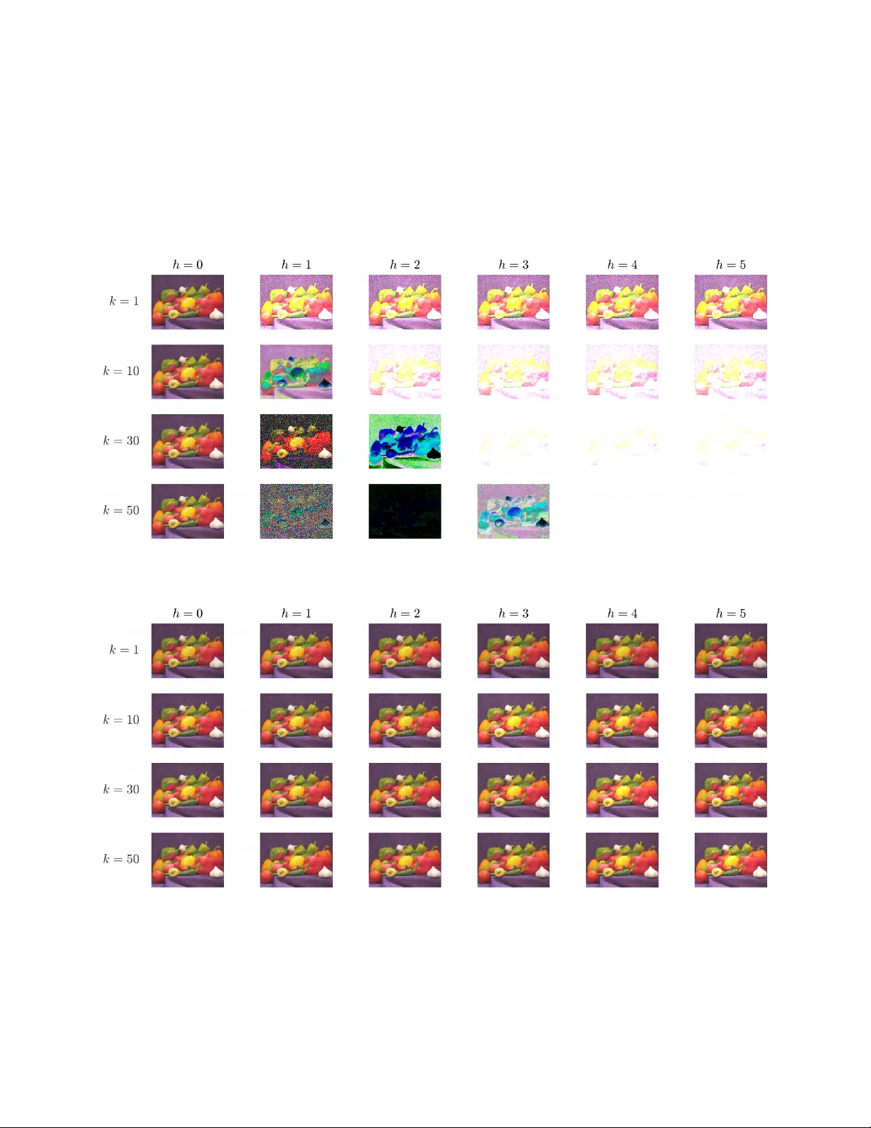
Structure, Analysis, and Syn thesis of First-Order Algorithms Jared Miller 1 , Carsten Sc herer 1 , F abian Jak ob 2 , Andrea Iannelli 2 Marc h 27, 2026 Abstract Optimization algorithms can b e in terpreted through the lens of dynamical systems as the intercon- nection of linear systems and a set of subgradien t nonlinearities. This dynamical systems formulation allo ws for the analysis and syn thesis of optimization algorithms by solving robust control problems. In this w ork, we use the celebrated internal mo del principle in con trol theory to structurally factorize con- v ergent comp osite optimization algorithms into suitable net work-dependent internal mo dels and core sub con trollers. As the key b eneﬁt, we reveal that this permits us to synthesize optimization algorithms ev en if information is transmitted ov er netw orks featuring dynamical phenomena such as time dela ys, c hannel memory , or crosstalk. Design of these algorithms is achiev ed under bisection in the exp onential con vergence rate either through a nonconv ex lo cal searc h or by alternation of con vex semideﬁnite pro- grams. W e demonstrate factorization of existing optimization algorithms and the automated syn thesis of new optimization algorithms in the netw orked setting. 1 In tro duction Comp osite optimization problems minimize a sum of functions ( f i ) s i =1 , as in β ∗ ∈ argmin β P s i =1 f i ( β ). These comp osite problems arise in applications such as regression [ 1 ], image denoising [ 2 ], matrix completion [ 3 ] and robust mo del predictive con trol [ 4 ]. These problems may also be solved o ver net w orks featuring dynamics such as time dela ys, channels with memory , or crosstalk [ 5 , 6 ]. Such net work dynamics could cause algorithms that are nominally conv ergent to no longer conv erge to an optimizer β ∗ . First-order optimization algorithm are pro cedures that ﬁnd an optima β ∗ of the comp osite optimization problem by using gradient/subdiﬀerential ev aluations of ∂ f i , without needing higher order information such as Hessians ∇ 2 f i [ 7 ]. First-order optimization algorithms can b e understo o d through a system-theoretic lens as the in terconnection b etw een memoryless nonlinearities ∂ f i and a linear system [ 8 , 9 , 10 ]. An example of suc h a comp osite optimization algorithm is Davis-Yin Splitting [ 11 ] with s = 3, where f 2 is smo oth (has Lipsc hitz gradients). Da vis-Yin Splitting with scalar parameters ( γ , λ ) has an algorithmic law of ω k = ( I + γ ∂ f 1 ) − 1 ( ζ k ) , ζ k + 1 2 = 2 ω k − ζ k − γ ∂ f 2 ( ω k ) , ζ k +1 = ζ k + λ ( I + γ ∂ f 3 ) − 1 ( ζ k + 1 2 ) − λω k . (1) J. Miller and C. Scherer are with the Chair of Mathematical Systems Theory , Departmen t of Mathematics, Universit y of Stuttgart, Stuttgart, German y ( { jared.miller, carsten.scherer } @imng.uni-stuttgart.de) F. Jakob and A. Iannelli are with the Institute for Systems Theory and Automatic Con trol, Univ ersity of Stuttgart, Germany (e-mail: { fabian.jakob, andrea.iannelli } @ist.uni-stuttgart.de). J. Miller and C. Scherer are funded b y Deutsche F orsch ungsgemeinschaft (DF G, German Research F oundation) under Germany’s Excellence Strategy - EXC 2075 – 390740016. J. Miller and C. Scherer ackno wledge the supp ort by the Stuttgart Center for Simulation Science (SimT ech). F. Jak ob ackno wledges the supp ort of the International Max Planck Research School for Intelligen t Systems (IMPRS-IS). Application of Davis-Yin Splitting in (1) to wards solving a composite optimization problem with v ariable β ∈ R c can b e expressed as the following interconnection of subgradient nonlinearities ( ∂ f 1 , ∂ f 2 , ∂ f 3 ) and a discrete-time linear system with time index k , state x , input w , and output z :      x k +1 z 1 k z 1 k z 1 k      =           1 − γ λ − γ λ − γ λ 1 − γ 0 0 1 − γ 0 0 1 − 2 γ − γ − γ      ⊗ I c           x k w 1 k w 2 k w 3 k      ,    w 1 k w 2 k w 3 k    ∈    ∂ f 1 ( z 1 k ) ∂ f 2 ( z 2 k ) ∂ f 3 ( z 3 k )    . (2) If the optimizer β ∗ is unique and the algorithm in (2) is conv ergen t, then the steady-state output sequence satisﬁes lim k →∞ ( z 1 k , z 2 k , z 3 k ) = ( β ∗ , β ∗ , β ∗ ) indep endent of the initial state x 0 . The problem of optimization algorithm design in this setting can be p osed as choosing a linear time- in v ariant system to connect to the subgradient nonlinearit y . The p erformance of an optimization algorithm can b e judged by its conv ergence rate to the optima β ∗ (e.g. exp onential conv ergence). This design task is made more diﬃcult when conv ergence to β ∗ m ust b e ensured in the presence of netw ork dynamics. Con vergen t algorithms must satisfy the following t wo prop erties: 1. Consensus: the same p oint β ∗ m ust b e sen t to every op erator ∂ f i ( ∀ i : z i = β ∗ ). 2. Optimality: The p oint β ∗ is optimal in the sense of 0 ∈ P s i =1 ∂ f i ( z i ). The Consensus requiremen t also emerges in distributed optimization [ 12 ], in which eac h of the separate comm unicating and computing agents m ust return the same v alue β ∗ . Obedience of the Consensus and Optimalit y constraints imp oses structural requirements on the linear system asso ciated with any conv ergent optimization algorithm [ 13 , 14 ]. These structural requiremen ts can b e interpreted as regulation and distur- bance rejection phenomena resp ectively [ 15 , 16 , 17 , 18 ] in the sense of control theory . Linear systems that satisfy the Consensus and Optimalit y requirements when in terconnected with a net w ork satisfy an aﬃne relation betw een their state-space matrices induced b y a regulator equation. The searc h ov er linear sys- tems when designing algorithms can therefore be restricted to linear systems that satisfy the relation, thus reducing the degrees of freedom in the design pro cedure. W e will show that regulation theory also giv es insigh ts into structural properties of optimization algo- rithms. Using an in ternal mo del principle [ 15 , 17 ], w e can factorize the linear system part of conv ergent optimization algorithms ov er netw orks in to the cascade of a core sub controller Σ core con taining the algo- rithm parameters, and an in ternal model Σ min that depends only on the net work. Because the Da vis-Yin algorithm can directly interface the subgradients ( ∂ f 1 , ∂ f 2 , ∂ f 3 ) without encoun tering net work dynamics, this particular internal mo del Σ min is an integrator that dep ends only on the dimensions s and c . The in ternal-mo del-based cascade factorization applied to the s = 3 Davis-Yin algorithm in (2) is Σ core :      ˜ u 1 , 1 k ˜ u 2 , 1 k ˜ u 2 , 2 k ˜ u 2 , 3 k      =           − γ λ − γ λ − γ λ − γ 0 0 − γ 0 0 − 2 γ − γ − γ      ⊗ I c         w 1 k w 1 k w 3 k    , (3a) Σ min :      x k +1 z 1 k z 2 k z 3 k      =           1 1 0 0 0 1 0 1 0 0 1 0 0 1 0 1 0 0 0 1      ⊗ I c              x k ˜ u 1 , 1 k ˜ u 2 , 1 k ˜ u 2 , 2 k ˜ u 2 , 3 k         . (3b) 2 The in ternal mo del factorization allo ws us to syn thesize optimization algorithms ov er net works b y solving structured robust control problems. These robust con trol problems arise by abstracting the subgradien t nonlinearit y into an uncertaint y , and describing the uncertaint y using the frameworks of Passivit y and In tegral Quadratic Constrain ts (IQCs) [ 19 ]. This principled search o ver Σ core also certiﬁes well-posedness and exp onential conv ergence rates of the resultant algorithm. 1.1 Literature Review The application of regulation theory and the in ternal model principle to w ards understanding optimization algorithms is a contin uation of existing uniﬁcations betw een con trol theoretic to ols and optimization (systems theory of algorithms [ 10 , 20 , 21 ]). Early use of dynamical systems to wards the analysis and solution of optimization algorithms include Lyapuno v interpretations of algorithmic conv ergence [ 22 , Section 10.4], pro vision of stability guaran tees in numerical in tegration [ 23 ], and solution of sorting and linear programming [ 24 ]. The w ork in [ 25 ] provides a systems-theoretic p ersp ective on linear and nonlinear ro otﬁnding algorithms. Dynamical-systems to ols that hav e b een used for the analysis and synthesis of optimization algorithms include gradient ﬂows [ 26 , 27 , 28 , 29 ], In tegral Quadratic Constrain ts (IQC) [ 30 , 19 ], dissipativity [ 31 , 32 ], and passivity [ 33 ]. The internal model principle was used in [ 34 , 35 ] to p erform p erfect tracking in online optimization. W e note that Scaled Relativ e Graphs [ 36 ], originally used to analyze conv ergence of optimization algorithms, hav e made the leap to dynamical systems for the analysis and con trol of nonlinear systems [ 37 ]. Optimization algorithms can b e deploy ed as controllers for cyb erphysical systems [ 38 ], such as in mo del predictive con trol [ 39 , 4 ]. The ﬁrst application of IQCs for the analysis of optimization algorithms o ccurred in [ 40 ] to analyze the asymptotic exponential con vergence rate of optimization algorithms. Prop erties of the oracle suc h as (strong) monotonicity , coco ercivit y , and Lipschitzness can b e mo deled as p oint wise (static) IQC constraints. When the oracle is the sub diﬀerential of a conv ex function, the subgradient inequalit y induces an inﬁnite set of dynamic O‘Shea-Zames-F alb multipliers [ 41 , 42 ], eac h of which expresses a dissipation relation that is v alid for all compatible oracles. Algorithm con vergence can b e tested through the solution of semideﬁnite programming problems, in volving a conv ex searc h o ver co eﬃcients that parameterize the multipliers. The con vergence rate of the algorithm can b e found through bisection by ﬁnding a minimal rate (up to numerical tolerance) at which the stability test fails to certify con v ergence. IQC theory was used to derive the T riple Momen tum scheme [ 43 ], which was prov en to b e optimal among all ﬁrst-order and ﬁxed-stepsize algorithms for strongly conv ex optimization in [ 44 ]. The optimality of T riple Momen tum was numerically certiﬁed using IQCs in [ 45 ]. Conserv atism in this IQC-based scheme arises through the ﬁnite order of the ﬁlters used: increasing the ﬁlter order raises computational complexity but may decrease the certiﬁed conv ergence rate. While determining conditions for which the true algorithm conv ergence rate is returned as the ﬁlter order increases remains an op en problem, the IQC-based approac h can (numerically) certify the optimality of algorithms suc h as gradient descent and triple momen tum at order-1 ﬁlters. Extensions of IQC analysis b ey ond static optimization algorithms include smo oth games [ 46 ], parameter-v arying optimization [ 47 ], and online optimization [ 48 ]. IQC and dissipativity to ols were used in [ 49 ] to determine conditions under whic h individual optimization algorithms could b e tied together into a distributed optimization algorithm under a ﬁxed Laplacian interconnection. Syn thesis of algorithms is a challenging task, and this diﬃculty is increased when comp osite optimization problem m ust be solved ov er a net work. The IQC-analysis method in [ 40 , 50 ] designed optimization algo- rithms based on a h yp erparameter search: choose algorithm parameters such that the IQC-deriv ed programs yield a minimal conv ergence rate. By mo deling the algorithm design task as a robust c on trol problem, clas- 3 sical con trol methods suc h as H ∞ optimization can b e lev eraged to generate controllers [ 51 ]. The w ork in [ 52 , 53 , 54 ] use frequency-domain metho ds to synthesize optimization algorithms in the absence of netw ork dynamics. The Consensus and Optimality prop erties are interpreted as tangental interpolation constrain ts of transfer function matrices [ 55 ]. Nev alinna-Pick interpolation theory [ 56 , 57 ] is then used to generate algo- rithms that satisfy the Consensus and Optimalit y constrain ts. This frequency-domain framew ork is extended to equality-constrained algorithms in [ 58 ] and distributed optimization algorithms in [ 53 ]. In the case of a single oracle (e.g. unconstrained optimization), the single-input-single-output structure of the controller leads to a p ossible commutation betw een the netw ork and the ﬁlters. This allows for conv ex syn thesis of the algorithm and the ﬁlter co eﬃcien ts, even in the netw orked setting [ 59 ]. The comm utation programs were ﬁrst presen ted using the Y oula-Kucera-Jabr [ 60 , 61 ] parameterization of all stabilizing con- trollers (algorithms) in [ 62 ], and later reformulated with direct state-space argumen ts in [ 63 ]. Algorithm design has been conducted for classes of switc hed systems (e.g. time-v arying delays in netw orks) in [ 64 ] through an alternating searc h betw een switch-mode-dep endent controllers and ﬁlter coeﬃcients. The w ork in [ 59 , 62 , 63 , 64 ] perform synthesis only in the case of a single oracle. The work in [ 65 ] uses Ly apunov argumen ts and general sector conditions to generate optimization algorithms for ﬁxed multipliers in the con- v ex and saddle-point case. The saddle point case considered in [ 65 ] includes a class of equalit y-constrained strongly conv ex problems, which can b e treated as a tw o-oracle problem. The P erformance Estimation Problem (PEP) approach is an alternativ e metho d for the analysis and syn thesis of optimization algorithms [ 66 ]. Giv en a set of v ariables corresp onding to a ﬁnite num b er of p oin ts, scalars, and vectors, the PEP approach uses interpolation constraints to describ e conditions for whic h a conv ex function exists with v alues at the p oints equal to the scalars and gradients equal to the v ectors. Queries suc h as the gradien t error, residual, or function decrease can b e exactly answered in a ﬁnite-horizon case b y solving semideﬁnite programming problems [ 67 ]. The PEP framew ork extends to establishing contraction rates for monotone inclusion schemes [ 68 ]. Optimal v ariable-step and ﬁxed-step rules for unconstrained gradien t descent of sm o oth conv ex functions w ere syn thesized using these int erp olation constrain ts in [ 44 ]. The w ork in [ 69 ] generates optimal step sizes through the branc h-and-b ound-based global optimization of nonconv ex quadratic programs. Interpolation constraints can b e used in asymptotic analysis of optimization algorithms: the w orks in [ 70 , 71 , 14 ] use Ly apunov arguments to certify con v ergence rates in which the uncertaint y is describ ed by interpolation constraints. 1.2 Con tributions W e ﬁrst provide a condition for conv ergence of a w ell-p osed optimization algorithm o ver a dynamical netw ork: the algorithmic in terconnection m ust satisfy a Regulator Equation and a Robust Stabilit y property . The Regulator Equation ma y b e veriﬁed by solving a linear system of equations. Certiﬁcation of the Robust Sta- bilit y prop erty is a challenging robust control problem inv olving system dynamics, and will b e approximated using a sequence of conv ex programs. W e then prov e a state-space in ternal mo del principle [ 15 ] for optimization algorithms, ensuring that any con vergen t net work ed optimization algorithm can b e split into a core sub controller Σ core and a netw ork- dep enden t internal mo del Σ min as in (3). Design of the ov erall algorithm inv olves searching ov er Σ core satisfying a structural constraint induced by the regulator equation. W e analyze existing algorithms and synthesize new algorithms by solving linear matrix inequalities (LMIs). Analysis and syn thesis b oth inv olve bisection ov er the exp onential con vergence rate. A t each ﬁxed conv ergence rate, Analysis inv olves searc hing o ver Zames-F alb ﬁlter coeﬃcients that deﬁne v alid re- lations satisﬁed by subgradien t nonlinearities. W e prop ose t wo paths for algorithm syn thesis to ﬁnd Σ core 4 at a ﬁxed con vergence rate. The ﬁrst path in volv es a nonconv ex searc h o ver reduced-order con trollers and ﬁlter co eﬃcien ts, leading to low-order and highly structured con trollers. The second path incorp orates a full-order internal mo del into system dynamics, and p erforms an alternating conv ex search ov e r v alid ﬁlter co eﬃcien ts parameterizing the IQC/passivity speciﬁcation. In each of these paths, feasibility of the resulting robust control problem ensures conv ergence of the optimization algorithm to the optimal p oint. The sp eciﬁc contributions of this work are • A tw o-part condition for conv ergence of optimization algorithms (Robust Stabilit y , Regulator Equa- tion). • A structural state-space factorization of conv ergent ﬁrst-order optimization algorithms based on the in ternal mo del principle with examples. • A synthesis framework for generating optimization algorithms ov er netw orks based on internal mo dels and linear matrix inequalities. • Demonstration of algorithm synthesis in the dynamical netw orked setting. T able 1 lists the main theoretical contributions of the pap er. T able 1: Main results of the paper Lemma 2.1 Suﬃcien t condition for well-posedness of optimization algorithms Theorem 3.1 Tw o-part condition for conv ergence of algorithms Theorem 4.1 Con troller order b ound based on well-posedness and information constraints Theorem 4.2 F actorization of optimization algorithms using the Internal Mo del Principle Theorem 5.1 LMI-based exp onential conv ergence rate analysis of well-posed algorithms Prop osition 5.3 LMI-based synthesis of certiﬁed well-posed exp onentially con verging algorithms This paper has the follo wing structure. Section 2 reviews preliminaries of notation, linear systems, conv ex analysis, and optimization algorithms. Section 3 pro vides a condition for the conv ergence of optimization algorithms using robust stabilit y and a regulator equation. Section 4 identiﬁes structural constrain ts on optimization algorithms and p erforms algorithm factorizations using an internal mo del principle. Section 5 p erforms automated synthesis of optimization algorithms based on solving nonconv ex or alternating-conv ex programs arising from robust control. Section 6 demonstrates our approach on example netw orked optimiza- tion tasks. Section 7 concludes the pap er. 2 Preliminaries W e ﬁrst review preliminaries of notation, linear systems, and optimization algorithms. 2.1 Notation and Linear Algebra The set of natural n umbers including zero is N = { 0 , 1 , 2 , . . . } . The set of integers b et ween a and b inclusive is { a, . . . , b } . The set of complex n umbers, real n um b ers, and integers are respectively C , R , and Z . The extended real line is ¯ R = R ∪ {−∞ , ∞} . The n -dimensional real Euclidean space is R n . The n -dimensional p ositiv e orthant is R n > := { ( x 1 , . . . , x n ) ∈ R n | x i > 0 ∀ i ∈ { 1 , . . . , n }} . The set of n × m matrices is R n × m . The set of n -dimensional symmetric matrices is S n with S n ⊂ R n × n . An empty matrix will b e denoted as [ · ] and an empty set as ∅ . 5 The transpose of a matrix M ∈ R m × n is M ⊤ . The rank of M is rank( M ). The null space of M is n ull( M ), and its range (column) space is ran( M ). If M is square ( m = n ), the symmetric part of M ∈ R n × n is Sym( M ) = 1 2 ( M + M ⊤ ) and its in verse is M − 1 . The sp ectral radius of a square matrix M is the maximal absolute v alue of any eigenv alue of M , and is denoted as ρ ( M ). M is Sch ur if ρ ( M ) < 1. M is an ti-Sch ur if all its eigenv alues λ ∈ C satisfy | λ | ≥ 1. If M is symmetric, its minimal and maximal eigenv alues are λ min ( M ) and λ max ( M ), resp ectively . The all zeros matrix is 0 m × n , the all ones vector is 1 s , and the identit y matrix is I s . Subscripts will b e omitted if the dimensions are clear from context. Giv en a v ector v , the square matrix constructed with v along its main diagonal and zeros e v erywhere else is diag( v ). The blo ck diagonal concatenation of a set of matrices is blkdiag( · , . . . , · ). 2.2 Linear Systems A discrete time signal x : N → R n is a time-indexed sequence ( x k ) k ∈ N . The unit shift op erator z acts on a sequence x as z x = z ( x k ) k ∈ N = ( x k +1 ) k ∈ N and ( z x ) 0 = 0. A linear system G is a mapping from an input signal u : N → R n u and an initial state x 0 ∈ R n to an output signal y : N → R n y as G : ( x 0 , u ) → y . In this pap er, linear systems G are describ ed with matrices ( A , B , C , D ) in the state-space as G : x k +1 y k ! = A B C D ! x k u k ! with an abbreviation of y = " A B C D # u. (4) The transfer matrix of the system G is the rational function T ( z ) = C ( z I − A ) − 1 B + D for z ∈ C . If a giv en rational function T ( z ) is represented as T ( z ) = C ′ ( sI − A ′ ) − 1 B ′ + D ′ , the tuple ( A ′ , B ′ , C ′ , D ′ ) is a realization of T ( z ). Realizations are generally nonunique. F or linear systems G 1 : ( x 1 0 , u ) → y and G 2 : ( x 2 0 , y ) → z with resp ective representations ( A 1 , B 1 , C 1 , D 1 ), ( A 2 , B 2 , C 2 , D 2 ), the cascade in terconnection of G 1 and G 2 is G 2 G 1 : (( x 1 0 , x 2 0 ) , u ) → z , z = G 2 ( G 1 ( u )). The blo c k-diagonal system formed b y G 1 : ( x 1 0 , u ) → y and G 2 : ( x 2 0 , y ) → z with y 1 = G 1 ( x 1 0 , u 1 ) , y 2 = G 2 ( x 2 0 , u 2 ) is blkdiag( G 1 , G 2 ) : (( x 1 0 , x 2 0 ) , ( u 1 , u 2 )) → ( y 1 , y 2 ). The w ell-p osed feedback interconnection b et ween systems G 1 : ( x 1 0 , ( w , u )) → ( z , y ) and G 2 : ( x 2 0 , ( y , a )) → ( u, b ) along their shared signals ( u, y ) is the star pr o duct G 1 ⋆ G 2 : (( x 1 0 , x 2 0 ) , ( w , a )) → ( z , b ). W ell-p osedness ensures that the shared signals ( u, y ) are unique given ( x 1 , x 2 , w , a ), and this is true if I − D 2 D 1 is in vertible. W e refer to App endix A for s tate-space form ulas of these interconnections based on representations of G 1 and G 2 . The represen tation ( A , B , C , D ) of G is stable if A is Sc hur. This holds iﬀ all tra jectories of (4) for u = 0 and any x 0 ∈ R n satisfy lim k →∞ x k = 0. The represen tation ( A , B , C , D ) of G is con trollable (stabilizable) or observ able (detectable) if ran  A − λI B  = n or null A − λI C ! = { 0 } (5) holds for all λ ∈ C ( λ ∈ C with | λ | ≥ 1), respectively , This will also be expressed b y sa ying that ( A , B ) is con trollable (stabilizable) or ( A , C ) is observ able (detectable). The order of a representation ( A , B , C , D ) is the dimension of A (which equals the n umber of states). The order of the transfer matrix of a system (called McMillan degree) is the minimum num b er of states required for a state-space realization thereof. A realization ( A , B , C , D ) is minimal iﬀ it is controllable and observ able. Let us ﬁnally recall that a controlled interconnection is describ ed by P :    x k +1 z k y k    =    A B 1 B 2 C 1 D 1 D 12 C 2 D 21 D 2       x k w k u k    , K : ξ k +1 u k ! = A c B c C c D c ! ξ k y k ! . (6) 6 Here P is the plant and K is the con troller. They share the control input u and the measurement output y . This special star pro duct is well-posed if E := I − D 2 D c is in vertible. W ell-p osedness p ermits elimination the common signals ( u, y ) , to arrive at the description    x k +1 ξ k z k    =       A 0 B 1 0 0 0 C 1 0 D 1    +    0 B 2 I 0 0 D 12    A c + B c E − 1 D 2 C c B c E − 1 ( I + D c E − 1 D 2 ) C c D c E − 1 ! 0 I 0 C 2 0 D 21 !    | {z }    A B C D       x k ξ k w k    . (7) W e refer to the interconnection in (6) as P ⋆ K , with the tacit understanding that it is well-posed and describ ed with the matrices in (7). The eliminated signals ( y , u ) can b e recov ered as y k u k ! = I − D 2 − D c I ! − 1 C 2 x k + D 21 w k C c ξ k ! . (8) Moreo ver, K internally stabilizes P if P ⋆ K is well-posed and if A is Sc hur stable. There exists a controller K which internally stabilizes P iﬀ ( A, B 2 ) is stabilizable and ( A, C 2 ) is detectable. 2.3 Con v ex Analysis W e review and deﬁne classes of functions, sub diﬀerentials, and op erators that are used to deﬁne optimization problems and optimization algorithms. 2.3.1 F unction Classes A function f : R c → ¯ R is proper if there exists a p oint x ∈ R c with f ( x ) < ∞ , and if f ( x ) > −∞ for all x ∈ R c [ 72 , Page 5]. The domain of a prop er function f is the set dom( f ) = { x ∈ R c | f ( x ) < ∞} and f is glob al ly deﬁne d if dom( f ) = R c . A prop er f is conv ex if ∀ ( x 1 , x 2 ) ∈ R c × R c , α ∈ [0 , 1] : f ( α x 1 + (1 − α ) x 2 ) ≤ αf ( x 1 ) + (1 − α ) f ( x 2 ), and it is close d if { x ∈ R c | f ( x ) ≤ α } is closed for eac h α ∈ R . A function that is prop er, conv ex, and closed will b e referred to as b eing p.c.c. A function f : R c → ¯ R is m -strongly conv ex with m > 0 if f − m 2 ∥·∥ 2 2 is conv ex. f is L -smo oth with L < ∞ if it is diﬀerentiable at every point x ∈ R c and if ∀ x, x ′ ∈ R c : ∥∇ f ( x ) − ∇ f ( x ′ ) ∥ ≤ L ∥ x ′ − x ∥ 2 . Deﬁne q ( x ) = 1 2 ∥ x ∥ 2 2 for x ∈ R c . Given m ∈ R , the set S m, ∞ comprises all functions f : R c → ¯ R such that f − m q is p.c.c. Moreov er, S m,L for L ∈ R consists of all f ∈ S m, ∞ suc h that L q − f is p.c.c.. Nonemptiness of S m,L requires that m ≤ L , and the only members of S m,m are the functions f = m q + g with aﬃne g : R c → R . If referring to the class S m,L , we will tacitly assume that −∞ < m < L ≤ ∞ from no w on. F or L = ∞ , this is an extension of existing deﬁnitions in [ 73 , 74 ] to the case where f is extended real-v alued, and to [ 75 , 65 ] when f is nonsmo oth. F or f ∈ S m,L , dom( f )  = ∅ is conv ex, since it equals dom( f − m q ). Note that S 0 , ∞ is the set of p.c.c. functions, and any f ∈ S m, ∞ for m > 0 is m -strongly conv ex [ 76 ]. If L < ∞ , all f ∈ S m,L are globally deﬁned (since f − m q and L q − f are prop er) and con tinuously diﬀeren tiable [ 63 , Lemma 3]; if m > 0 then f is L -smo oth and m -strongly-conv ex. The indicator function of a set Z ∈ R c is deﬁned as I Z ( x ) = 0 if x ∈ Z and I Z ( x ) = ∞ if x ∈ Z . If Z  = ∅ is closed and conv ex, then I Z ∈ S 0 , ∞ . The aﬃne hull of a set Z is the smallest aﬃne space containing Z (in tersection of all aﬃne spaces including Z ). Its relative interior is the interior of Z viewed as a subset of its aﬃne hull [ 72 , Section 2.H]. Figure 1 visualizes the contours of four example functions inside S m,L within the domain [ − 3 , 3] 2 . 7 Figure 1: Con tours plotted of functions in S m,L with c = 2. 2.3.2 Sub diﬀeren tials The sub diﬀerential of a p.c.c. function f at x ∈ R c is deﬁned as ∂ f ( x ) = { g ∈ R c | f ( x ′ ) ≥ f ( x ) + g ⊤ ( x ′ − x ) ∀ x ′ ∈ R c } . (9) The F rech ´ et subdiﬀerential of a function f ∈ S m,L is ∂ f := ∂ ( f − m q ) + mI , where ∂ ( f − m q ) is the standard sub diﬀeren tial of the p.c.c.function f − m q ([ 77 , Deﬁnition 6.2, (iii)] using [ 78 , Prop osition 1.107 (i)]). S 0 m,L is the subset of functions f ∈ S m,L whic h are zero-centered as 0 = f (0) and 0 ∈ ∂ f (0). As examples, ∂ I Z is the normal cone op erator for Z , and ∂ f ( x ) = {∇ f ( x ) } holds for all x ∈ R c if f ∈ S m,L and L < ∞ . The identit y function I : R c → R c , I ( x ) = x , satisﬁes I = ∂ q . Figure 2 plots an example of the sub diﬀerential of functions in S m,L for the m -parameterized function g m ( β ) := max  1 2 | β − 1 2 | , 3 | β − 1 2 | − 4  + m 2 ∥ β + 1 . 1 ∥ 2 2 , (10) in whic h g m ∈ S m, ∞ for all m ∈ R . The blue (top) and orange (b ottom) curv es dra w the conv ex g 0 ( β ) and the noncon vex g − 1 ( β ), respectively . The blac k arrows visualize v ectors in the respective multiv alued sub diﬀeren tials ∂ g m ( β ) at β = 2 . 1. -4 -3 -2 -1 0 1 2 3 4 - -3 -2 -1 0 1 2 3 4 5 g m ( - ) g 0 g ! 1 @ g Figure 2: F unctions g m in (10) and vectors inside ∂ g m (2 . 1) for m ∈ {− 1 , 0 } . 8 2.3.3 Op erators An operator is a set-v alued map F : R c ⇒ R c [ 72 , 76 ]. Its in verse is deﬁned as F − 1 ( x ) := { y ∈ R c | x ∈ F ( y ) } for x ∈ R c . A matrix D ∈ R c × c is iden tiﬁed with the linear map x 7→ Dx for an y x ∈ R c . In this paper, ( I + D F ) − 1 is referred to as a generalized resolven t, and ( F − 1 − D ) − 1 is referred to as the generalized Y osida op erator. If D = − λI with λ > 0, a generalized Y osida op erator is related to the standard resolv ent ( I + λF ) − 1 through the inv erse resolv ent identit y [ 72 , Lemma 12.14] ( F − 1 + λI ) − 1 = λ − 1 [ I − ( I + λF ) − 1 ]. F is said to b e globally single-v alued if, for every x ∈ R c , F ( x ) consists of exactly one element, which is also denoted as F ( x ). F is said to b e globally contin uous if F is globally single-v alued and if the corresp onding map F : R c → R c , x 7→ F ( x ) is contin uous. If f ∈ S m,L then ∂ f : R c ⇒ R c is a set-v alued map. If m > 0, then f is strongly conv ex, which implies that ( ∂ f ) − 1 is globally contin uous. F or f ∈ S 0 , ∞ , we also recall that ( I + γ ∂ f ) − 1 is the proximal mapping z 7→ arg min z ∈ R c f ( z ) + 1 2 γ ∥ x − z ∥ 2 2 . The set of sub diﬀerentials to S m,L is ∂ S m,L = { ∂ f | f ∈ S m,L } . W e refer to App endix B for further details. 2.4 Comp osite Optimization Problems Giv en s ∈ N functions f i ∈ S m i ,L i for i ∈ { 1 , . . . , s } , a composite optimization problem amounts to ﬁnding a p oint β ∗ ∈ R c with β ∗ ∈ arg min β ∈ R c s X i =1 f i ( β ) . (11) An example of comp osite optimization arises from constrained minimization of a function f ∈ S m f ,L f with L f < ∞ on a closed conv ex set Z ⊂ R c . If w e choose f 1 = f and f 2 = I Z ∈ S 0 , ∞ , we infer that f 1 ( x ) + f 2 ( x ) = f ( x ) < ∞ holds iﬀ x ∈ Z , and hence (11) is equiv alent to β ∗ ∈ arg min x ∈Z f ( x ). This pap er studies algorithms solving the following zero inclusion problem. Problem 1 (Comp osite Optimization) . Given s ∈ N functions f i ∈ S m i ,L i for i ∈ { 1 , . . . , s } , ﬁnd a p oint β ∗ ∈ R c which satisﬁes 0 ∈ s X i =1 ∂ f i ( β ∗ ) . (12) If m 1 + · · · + m s > 0, Problem 1 has a unique optimal solution since the cost P s i =1 f i is prop er, closed and strongly conv ex. By Corollary B.1, an y solution β ∗ satisfying (12) is a solution of (11). If the domains of the functions are compatible according to relin t(dom( f 1 )) ∩ · · · ∩ relint(dom( f s ))  = ∅ , (13) then a solution β ∗ of (11) also satisﬁes (12). Again by Corollary B.1 and without constrain ts on m 1 , . . . , m s , an y lo cal solution of (11) also solves Problem 1. F or these reasons, w e refer to (12) as an optimalit y condition for the comp osite optimization problem (11). With the function f ( z ) := f 1 ( z 1 ) + · · · + f s ( z s ) for z = ( z 1 , . . . , z s ) ∈ R sc , the optimalit y condition (12) reads as 0 ∈ ( 1 s ⊗ I c ) ⊤ F ( 1 s ⊗ β ∗ ) inv olving the op erator F := ∂ f . Observ e that F can b e considered as a concatenation of the sub diﬀeren tials ∂ f 1 , . . . , ∂ f s , since F ( z ) =     F 1 ( z 1 ) . . . F s ( z s )     =     ∂ f 1 ( z 1 ) . . . ∂ f s ( z s )     :=            g 1 . . . g s     | g i ∈ ∂ f i ( z i ) , i ∈ { 1 , . . . , s }        . (14) In this pap er, w e work with the following classes of op erators. 9 Deﬁnition 1. Given ve ctors m = ( m 1 , . . . , m s ) and L = ( L 1 , . . . , L s ) , let O m,L b e the class of al l op er ators F in (14) for which (12) has a unique solution β ∗ ∈ R c and ther e exists a unique w ∗ ∈ F ( 1 s ⊗ β ∗ ) with ( 1 s ⊗ I c ) ⊤ w ∗ = 0 . Mor e over, O 0 m,L is the subset of al l op er ators F ∈ O m,L satisfying 0 ∈ ∂ f i (0) and f i (0) = 0 for i ∈ { 1 , . . . , s } , implying that 0 ∈ F (0) . 2.5 Optimization Algorithms Time-indep enden t iterativ e sc hemes to solv e Problem 1 can be expressed as a linear time-in v ariant system G represented by ( A , B , C , D ) in terconnected with the static map F ∈ O m,L as x k +1 z k ! = A B C D ! x k w k ! , w k ∈ F ( z k ) . (15) This feedback interconnection is depicted as a blo ck-diagram shown in Figure 3. F " A B C D # w z Figure 3: Standard algorithmic in terconnection in (15) Examples of optimization algorithms are Gradient Descent x k +1 = x k − α ∇ f ( x k ) represented as x k +1 z k ! = " 1 − α 1 0 ! ⊗ I c # x k w k ! , w k = ∇ f ( z k ) , (16) and the Davis-Yin algorithm [ 11 ] in (2). The following deﬁnition of a ﬁxed p oint of an algorithm is standard. Deﬁnition 2. A ﬁxe d p oint of (15) is a tuple ( x ∗ , z ∗ , w ∗ ) satisfying x ∗ z ∗ ! = A B C D ! x ∗ w ∗ ! , w ∗ ∈ F ( z ∗ ) . (17) This leads us to the following notion of algorithm conv ergence used in this pap er. Deﬁnition 3. The algorithmic inter c onne ction in (15) with F ∈ O m,L is a c onver gent optimization algorithm for Pr oblem 1 with solution β ∗ if ther e exists a ﬁxe d p oint ( x ∗ , w ∗ , z ∗ ) of (15) which satisﬁes the fol lowing thr e e pr op erties: Consensus: z ∗ = 1 s ⊗ β ∗ , (18a) Optimality: ( 1 s ⊗ I c ) ⊤ w ∗ = 0 , (18b) A ttr activity: ∀ x 0 ∈ R n : lim k →∞ ( x k , w k , z k ) = ( x ∗ , w ∗ , z ∗ ) . (18c) 10 Remark 2.1. Our class of c onsider e d pr oblems in the deﬁnition of O m,L and the attr activity pr op erty in (18c) r e quir es that ther e is a unique tuple ( β ∗ , w ∗ ) with w ∗ ∈ F ( 1 s ⊗ β ∗ ) , ( 1 ⊤ s ⊗ I c ) w ∗ = 0 . A suﬃcient c ondition for w ∗ to b e unique given the existenc e of a unique β ∗ solving Pr oblem 1 is if at most one index i ∈ { 1 , . . . , s } satisﬁes L i = ∞ . If ( A , C ) is dete ctable, then uniqueness of x ∗ fol lows, b e c ause ther e is at most one x ∗ such that A − I C ! x ∗ = −B w ∗ 1 s ⊗ β ∗ − D w ∗ ! . (19) 2.6 W ell-P osedness and Algorithm Execution The algorithm (15) inv olves the implicit constraint z k = C x k + D w k , w k ∈ F ( z k ). This translates into the equiv alent inclusions C x k + D w k ∈ F − 1 ( w k ) and w k ∈ ( F − 1 − D ) − 1 ( C x k ), whic h motiv ates the follo wing deﬁnition of well-posedness. Deﬁnition 4. The algorithm (15) is wel l-p ose d if the gener alize d Y osida op er ator H := ( F − 1 − D ) − 1 is glob al ly c ontinuous. If (15) is w ell-p osed, it can b e rewritten as an explicit recursion x k +1 = A x k + B H ( C x k ) with outputs w k = H ( C x k ) , z k = C x k + D H ( C x k ) for all k ∈ N . (20) W ell-p osedness implies that tra jectories ( x k , w k , z k ) k ∈ N exist and are unique for ev ery x 0 ∈ R n . In the sequel, we refer to the algorithm as F ⋆ G (represented by (15)), with the tacit understanding that it is w ell-p osed (and can also b e expressed as (20)). W e note that F ⋆ G ma y b e well-posed but not con vergen t. F or example, the subgradient descen t scheme z k +1 ∈ z k − γ ∂ f ( z k ) is not w ell-p osed if γ  = 0 and if f is not diﬀerentiable ev erywhere. On the other hand, w ell-p osedness implies uniqueness of the ﬁxed p oint in con vergen t algorithms. Prop osition 2.1. If the algorithm (15) is wel l-p ose d and ther e exists some ve ctor x ∗ with lim k →∞ x k = x ∗ for al l initial c onditions x 0 , then (15) admits a unique ﬁxe d p oint ( x ∗ , z ∗ , w ∗ ) and al l its tr aje ctories satisfy lim k →∞ ( x k , w k , z k ) = ( x ∗ , w ∗ , z ∗ ) . Pr o of. Since H in (20) is contin uous, by taking the limit k → ∞ we infer x ∗ = A x ∗ + B H ( C x ∗ ) and lim k →∞ w k = H ( C x ∗ ) =: w ∗ as w ell as lim k →∞ z k = C x ∗ + D H ( C x ∗ ) =: z ∗ . Hence w ∗ = A x ∗ + B w ∗ and C x ∗ ∈ H − 1 ( w ∗ ) = F − 1 ( w ∗ ) − D w ∗ , i.e., z ∗ = C x ∗ + D w ∗ ∈ F − 1 ( w ∗ ) and th us w ∗ ∈ F ( z ∗ ). This shows that ( x ∗ , w ∗ , z ∗ ) is a ﬁxed p oint of (15) and lim k →∞ ( x k , w k , z k ) = ( x ∗ , z ∗ , w ∗ ). An y other ﬁxed p oint ( ¯ x ∗ , ¯ w ∗ , ¯ z ∗ ) of (15) satisﬁes ¯ x ∗ = A ¯ x ∗ + B ¯ w ∗ , ¯ z ∗ = C ¯ x ∗ + D ¯ w ∗ and ¯ w ∗ ∈ F ( ¯ z ∗ ); hence C ¯ x ∗ ∈ F − 1 ( ¯ w ∗ ) − D ¯ w ∗ and th us ¯ w ∗ = H ( C ¯ x ∗ ), whic h giv es ¯ x ∗ = A ¯ x ∗ + B H ( C ¯ x ∗ ) as w ell as ¯ z ∗ = C ¯ x ∗ + H ( C ¯ x ∗ ). If w e initialize a tra jectory of (20) as x 0 = ¯ x ∗ , it hence satisﬁes x k = ¯ x ∗ for all k ∈ N ; b y assumption, w e ha ve lim k → x k = x ∗ whic h implies ¯ x ∗ = x ∗ and hence also ( ¯ x ∗ , ¯ w ∗ , ¯ z ∗ ) = ( x ∗ , w ∗ , z ∗ ). Unfortunately , the ev aluation of H may b e as c hallenging as solving the original optimization problem (12). This diﬃculty could b e due to the p ossible requiremen t of solving implicit nonlinear ﬁxed p oint equations. If D admits a low er-triangular blo ck structure (p ossibly after a p ermutation of ( f 1 , . . . , f s )), the ev aluation of H can b e achiev ed with the generalized resolv en ts of ∂ f i for i ∈ { 1 , . . . , s } . T o perform this algorithm ev aluation, we partition B = ( B i ), C = ( C i ) and D = ( D ij ) from (15) into c × c blo c ks to form the 11 represen tation A B C D ! =          A B 1 B 2 . . . B s C 1 D 11 0 . . . 0 C 2 D 21 D 22 . . . 0 . . . . . . . . . . . . . . . C s D s 1 D s 2 . . . D ss          , (21) and we deﬁne the generalized Y osida op erators as H i := ( ∂ f − 1 i − D ii ) − 1 for each i ∈ { 1 , . . . , s } . Lemma 2.1. An algorithm (15) with D having a blo ck-lower-triangular structur e as p artitione d in (21) is wel l-p ose d if the diagonal blo cks D ii satisfy Sym(( σ i L i D ii − σ i I ) ⊤ ( I − m i D ii )) ≺ 0 with σ i := ( L i − m i ) − 1 for i ∈ { 1 , . . . , s } . (22) If L i = ∞ , then σ i L i = 1 and σ i = 0 , which implies that (22) sp e cializes to D ii + D ⊤ ii − 2 m i D ⊤ ii D ii ≺ 0 . (23) The r e cursion in (20) admits the explicit description starting fr om an initial c ondition x 0 ∈ R n as fol lows: Determine w i k = H i  C i x k + P i − 1 j =1 D ij w j k  for i = 1 , 2 , . . . , s in asc ending or der (24) and set x k +1 = A x k + P s i =1 B i w i k . Pr o of. The relation w ∈ ( F − 1 − D ) − 1 ( z ) is equiv alent to z = x + D w , w ∈ F ( z ). In a partition of the vectors ( w , z ) compatible to the index i ∈ { 1 , . . . , s } of the blocks of D in (21), the vector z can b e expressed as z i = C i x i + P i − 1 j =1 D ij w j + D ii w i , w i ∈ F i ( z i ) for i ∈ { 1 , . . . , s } . (25) Since F ∈ O m,L implies F i = ∂ f i ∈ ∂ S m i ,L i , Corollary B.4 assures that H i = ( F − 1 i − D ii ) − 1 is globally con tinuous under condition (22). Therefore, (25) is equiv alent to w i = H i  C i x + P i − 1 j =1 D ij w j  for i ∈ { 1 , . . . , s } . (26) This represen tation of w ∈ ( F − 1 − D ) − 1 ( z ) prov es that H = ( F − 1 − D ) − 1 is globally contin uous, and hence the algorithm is well-posed. Moreov er, (26) leads to (24) and hence to an explicit algorithm description. W e emphasize a few sp ecial cases based on Corollary B.3: 1. If ∂ f i is globally contin uous (e.g. for L i < ∞ in which ∂ f i = ∇ f i ), then H i ( v ) =    ∇ f i ( v ) if D ii = 0 , ∇ f i (( I − D ii ∇ f i ) − 1 ( v )) if D ii  = 0 . (27) 2. If ∂ f i ( β ) is not single-v alued at some β ∈ R c , then L i is not ﬁnite. In this case, w e can ev aluate the generalized Y osida op erator H i using the generalized resolv ent ( I + D ii ∂ f i ) − 1 as H i = D − 1 ii [ I − ( I + D ii ∂ f i ) − 1 ], noting that (23) implies inv ertibility of D ii . 3. If D ii is diagonal with D ii = λ i I and L i = ∞ , then condition (23) requires that λ i ∈ ( −∞ , 0) ∪ (1 /m i , ∞ ) if m i > 0, λ i ∈ ( −∞ , 0) if m i = 0, and λ i ∈ (1 /m i , 0) if m i < 0. 12 2.7 Kronec k er Structure Most ﬁrst-order optimization algorithms hav e a Kroneck er structure [ 79 ]. Deﬁnition 5. A system in (15) has Kr one cker Structur e if ther e exists matric es ( A a , B a , C a , D a ) with A B C D ! = A a B a C a D a ! ⊗ I c . (28) Examples are the Davis-Yin algorithm (1) and Gradien t descent (16). The pro cedure in [ 14 , Proposition 2] is an instance of (24) when the algorithm is Kroneck er structured. W e will use the sup erscript a to denote matrices that hav e a Kroneck er structure (e.g. A a with A a ⊗ I c = A in (28)). F urthermore, we will use the Kronec ker pro duct to denote Kroneck er-structured linear systems, using the notation G = G a ⊗ I : x k +1 y k ! = A a B a C a D a ! ⊗ I c ! x k u k ! abbreviated as y = " A B C D # ⊗ I c ! u. (29) 2.8 Algorithms ov er Netw orks The algorithm (15) in v olves a linear system G directly interconnected to the op erator oracle F . Design of optimization algorithms may also o ccur in settings where the oracle F is not directly accessible. Example instances include time dela ys, pack et drops, and netw ork cross-talk [ 6 ]. W e mo del this setting by assuming that G is given by the interconnection of a netw ork (or plant) P :    x N k +1 z k y k    =    A B 1 B 2 C 1 D 1 D 12 C 2 D 21 D 2       x N k w k u k    , (30) with a controller K with n y inputs and n u outputs as describ ed b y K : ξ k +1 u k ! = A c B c C c D c ! ξ k y k ! . (31) If E := I − D 2 D c is inv ertible, w e recall that this interconnection is well-posed and admits a state-space description with ( A , B , C , D ) deﬁned b y (7), which is referred to as P ⋆ K . F or G = P ⋆ K , the algorithmic interconnection F ⋆ G = F ⋆ ( P ⋆ K ) is visualized b y blo ck-diagrams in Figure 4. These rev eal ho w the (given and ﬁxed) netw ork P bridges the oracle F and the (to be designed con troller) K to generate the algorithm F ⋆ ( P ⋆ K ). The sp eciﬁc c hoice P 0 : z k y k ! = 0 I cs I cs 0 ! w k u k ! (32) reco vers a direct interconnection, since then P 0 ⋆ K = K and G is just equal to the con troller K . Example 2.1. The Kr one cker-structur e d pr oximal p oint metho d z k +1 = ( I + γ ∂ f ) − 1 ( z k ) for f ∈ S m,L and γ > 0 may b e describ e d as an inter c onne ction ∂ f ⋆ K pr ox with K pr ox : x k +1 z k ! = I − γ I I − γ I ! x k w k ! . (33) The left inter c onne ction of Figur e 5 intr o duc es a delay of 1 time step b efor e and after the c omputation of ∂ f . The right inter c onne ction assembles the 1-step channel delays into a network P sitting b etwe en 13 F    A B 1 B 2 C 1 D 1 D 12 C 2 D 21 D 2    " A c B c C c D c # w z y u F " A B C D # w z Figure 4: Blo ck diagrams of an algorithm o ver a net work giv en b y F ⋆ ( P ⋆ K ) (left) and its closed-loop represen tation F ⋆ G (righ t) with G = P ⋆ K represented b y ( A , B , C , D ). ∂ f      0 0 I 0 0 0 0 I 0 I 0 0 I 0 0 0      " I − γ I I − γ I # w z y u ∂ f " I − γ I I − γ I # Dela y 1 Dela y 1 w y z u Figure 5: Proximal p oint metho d in (33) dela yed by one time step (left) and the net work representation (righ t) ∂ f and K pr ox . The inter c onne ction F ⋆ ( P ⋆ K pr ox ) c an as wel l b e describ e d by the algorithmic pr o c e dur e z k +1 = z k − γ ∇ f ( z k − 1 ) , z ′ k +1 = z k − γ ∇ f ( z k − 1 ) , in which z ′ is an unobservable state. Figur e 6 visualizes the exe cution of ∂ f ⋆ K pr ox (top) and ∂ f ⋆ ( P ⋆ K pr ox ) (b ottom) with p ar ameter γ = 5 when minimizing the function f ( β ) = ∥ β − β 0 ∥ 2 2 . The term β 0 ∈ R 10 with β ∗ = β 0 is r andomly sele cte d. The left plot dr aws the err or z k − β ∗ for k ∈ { 0 , . . . , 14 } in the nominal exe cution ∂ f ⋆ K pr ox . The c onver genc e of the nominal exe cution ∂ f ⋆ K pr ox is demonstr ate d by the err or going to zer o. The err or z k − β ∗ diver ges to ∞ in the delaye d exe cution ∂ f ⋆ ( P ⋆ K pr ox ) in the right plot. The intr o duction of delays ther efor e destabilizes the nominal ly c onver gent algorithm. This destabilization gener alizes to networks with multiple delays. L etting P h denote a network with an h -step delay b efor e and after ∂ f , The c olor e d curves in Figur e 7 ar e plots of the sp e ctr al r adius of the matrix A cl := 1 ⋆ ( P h ⋆ K pr ox ) for h ∈ { 0 , . . . , 4 } as a function of γ . Conver genc e to β 0 for the function f ( β ) = 1 2 ∥ β − β 0 ∥ 2 2 is assur e d if the curve stays b elow the black dotte d line ( ρ = 1) . Without delays ( h = 0 ), the pr oximal p oint algorithm is c onver gent if γ > 0 . The h = 1 inter c onne ction is c onver gent if γ ∈ (0 , 1) . Incr e asing the delay shrinks the set of c onver gent γ values. 14 0 2 4 6 8 10 12 14 k -10 -5 0 5 10 z ! - $ No delay 0 2 4 6 8 10 12 14 k -4 -2 0 2 4 z ! - $ # 10 6 One-step delay Figure 6: Nominal and one-step-dela yed proximal p oin t metho ds to minimize f ( β ) = ∥ β − β 0 ∥ 2 2 . 0 0.5 1 1.5 2 2.5 3 3.5 4 4.5 5 . 0 0.5 1 1.5 2 2.5 ; ( A cl ) Conv e rgent Not Conv ergent No Delay Delay 1 Delay 2 Delay 3 Delay 4 ; = 1 Figure 7: Spectral radius of A cl v.s. algorithm parameter γ for the delay ed v ersion of (33) 2.9 Information Constraints The blo ck-sparsit y pattern of D deﬁnes an information structur e of the algorithm, sp ecifying the co ordinate v alues w j k of the sub diﬀerentials that may b e used to compute the other sub diﬀerential co ordinates w i k within the same iteration k ∈ N . Descriptions and labels for the eight p ossible sparsity patterns of the blo c k-low er-triangular matrices D for s = 2 are listed in T able 2, in whic h • indicates a p ossibly nonzero D ij submatrix. Sequen tial P arallel Pure Y osida • 0 • • ! • 0 0 • ! Mixed Y osida and Gradient 0 0 • • ! , • 0 • 0 ! 0 0 0 • ! , • 0 0 0 ! Pure Gradient 0 0 • 0 ! 0 0 0 0 ! T able 2: Blo ck-lo wer-triangular sparsity patterns of D for s = 2 15 In T able 2, an algorithm is ‘parallel’ if all w i co ordinates for the subgradien t can b e ev aluated indep en- den tly (blo ck-diagonal D ), or ‘sequential’ if there are dep endencies in w i computation. The algorithm F ⋆ ( P ⋆ K ) may b e restricted to satisfy an information constraint. An example includes the requirement that the matrix D from G = P ⋆ K must b e blo c k-low er-triangular, in order to admit ev aluation by the pro cedure in (24). More generally , we c ho ose a set L info ⊆ R n u × n y suc h that D c ∈ L info implies that the algorithm F ⋆ ( P ⋆ K ) obeys a desired information constraint on D . Imp osition of con vex information constrain ts on D could result in noncon vex sets sets L info , b ecause the expression D = D 1 + D 12 ( I − D c D 2 ) − 1 D c D 21 from (7) is nonlinear in D c if D 2  = 0. 2.10 Algorithm Synthesis Algorithm synthesis inv olves the design of a controller K such that F ⋆ ( P ⋆ K ) is a conv ergent optimization algorithm for all F ∈ O m,L , and that K ob eys the information structure constrain t expressed as D c ∈ L info . The formal description of the algorithm synthesis task is as follows: Problem 2 (Algorithm Synthesis) . Given a network P fr om (30) , an op er ator tuple O m,L , and a set L info , ﬁnd a c ontr ol ler K with r epr esentation ( A c , B c , C c , D c ) wher e D c ∈ L info and such that the inter c onne ction F ⋆ ( P ⋆ K ) is a wel l-p ose d c onver gent optimization algorithm for any F ∈ O m,L . The goal of this paper is to derive structural conditions on any con troller K whic h solves the syn thesis problem. This p ermits to search ov er con trollers K that satisfy these structural conditions to ﬁnd rapidly (exp onen tially) con verging algorithms. The structural constrain ts on K will be deriv ed using principles of regulation theory for linear systems. 2.11 Regulation Theory for the Rejection of Constant Disturbances Output regulation of linear systems inv olves the rejection of exogenous signals d with kno wn dynamics. W e fo cus on the case where the exogenous system generates constant signals d k = d 0 for all k ∈ N and refer to [ 15 , 16 , 80 ] for further information on regulation in control theory , including non-constan t disturbances. Consider the following linear system driven by a constan t disturbance d 0 ∈ R n d : ˜ G : x k +1 e k ! = ˜ A ˜ B ˜ C ˜ D ! x k d k ! , d k +1 = d k . (34) Deﬁnition 6. The system in (34) attains output r e gulation if ˜ A is Schur, and for al l x 0 ∈ R n , d 0 ∈ R n d , it holds that lim k →∞ e k = 0 . A core condition for output regulation is the feasibilit y of the so-called regulator equation. Lemma 2.2 (Lemma 1 [ 15 ]) . The system ˜ G with r epr esentation ( ˜ A , ˜ B , ˜ C , ˜ D ) achieves output r e gulation iﬀ the fol lowing two c onditions hold: 1. Stability: lim k → 0 x k = 0 for al l x 0 ∈ R n if d 0 = 0 . 2. Solvability of R e gulator Equation: Ther e exists a matrix Υ satisfying ˜ A − I ˜ B ˜ C ˜ D ! Υ I ! = 0 . (35) 16 Pr o of. W e provide this pro of for the purpos e of illustration. The stabilit y condition is met iﬀ ˜ A is Sch ur. If true, ( ˜ A − I ) has full rank and there exists a unique solution Υ to ˜ A Υ + ˜ B − Υ = 0 (top row of (35)). The system in (34) ma y b e describ ed by an extended system ˜ G ext with states ( x, d ). Performing the co ordinate c hange ( ˆ x, ˆ d ) = ( x − Υ d, d ) on the system ˜ G ext sho ws ˜ G ext :    x k +1 d k +1 e k    =    ˜ A ˜ B 0 I ˜ C ˜ D    x k d k ! ⇐ ⇒    ˆ x k +1 ˆ d k +1 e k    =    ˜ A ( ˜ A − I )Υ + ˜ B 0 I ˜ C ˜ C Υ + ˜ D    ˆ x k ˆ d k ! . (36) Giv en that ˜ A is Sch ur and ( ˜ A − I )Υ + ˜ B = 0, the state ˆ x k +1 satisﬁes lim k →∞ ˆ x k = 0 for all initial conditions ˆ x 0 . The steady-state v alue of e is lim k →∞ e k = lim k →∞ ˜ C ˆ x k + ( ˜ C Υ + ˜ D ) ˆ d k = ( ˜ C Υ + ˜ D ) d 0 . Hence, output regulation holds iﬀ ˜ C Υ + ˜ D = 0 since, otherwise, lim k →∞ e k  = 0 for some d 0  = 0. App endix C details the consequences of this result if (34) is a controlled interconnection. 3 Con v ergence of Optimization Algorithms The net work ed algorithm synthesis task (Problem 2) ma y be p osed as an instance of stabilization under regulation constraints [ 81 , 82 ]. T o this end, we conv ert the algorithmic interconnection F ⋆ ( P ⋆ K ) with ﬁxed p oint ( x ∗ , w ∗ , z ∗ ) into an error system ˜ F ⋆ ( P ⋆ K ) with some ˜ F ∈ O 0 m,L ha ving the ﬁxed p oint (0 , 0 , 0). With the regulation error e := z − 1 s ⊗ β ∗ , the consensus condition of a conv ergen t algorithm F ⋆ ( P ⋆ K ) is translated in to the regulation requiremen t lim k → 0 e k = 0. The latter property needs to b e guaranteed for the error system ˜ F ⋆ ( P ⋆ K ) that is aﬀected b y unknown constant disturbances whic h dep end on the unkno wn solution β ∗ of (12). In this fashion, algorithm conv erges is translated into such a regulation prop erty and global attractivity of the ﬁxed p oint (0 , 0 , 0) of the error system ˜ F ⋆ ( P ⋆ K ). 3.1 Error F orm ulation T o capture the optimality condition (18b), we introduce a so-called consensus matrix. Deﬁnition 7. A matrix N is a c onsensus matrix if N ∈ R sc × ( s − 1) c , rank( N ) = ( s − 1) c and ran( N ) = null(( 1 s ⊗ I c ) ⊤ ) . (37) A particular choice is N = I s − 1 − 1 ⊤ s ! ⊗ I c , such as N =   1 0 0 1 − 1 − 1   ⊗ I c for s = 3. When s = 1, the consensus matrix is omitted by setting N = [ · ]. Solutions β ∗ of Problem 1 can then b e characterized by 0 ∈ F ( 1 s ⊗ β ∗ ) − N ˆ w ∗ for some ˆ w ∗ ∈ R ( s − 1) c . (38) Let us partition g := N ˆ w ∗ ∈ R sc as g = col( g 1 , . . . , g s ) with g i ∈ ∂ f i ( β ∗ ) and associate to f i the zero- cen tered function ˜ f i ( z ) := f i ( z + β ∗ ) − f i ( β ∗ ) − ( g i ) ⊤ z with ˜ f i ∈ S 0 m,L for i ∈ { 1 , . . . , s } . Then the function ˜ f ( z ) := P s i =1 ˜ f i ( z i ) for z = ( z 1 , . . . , z s ) ∈ R sc leads to the error op erator ˜ F := ∂ ˜ f ∈ O 0 m,L , which satisﬁes ˜ F ( ˜ z ) = F ( ˜ z + 1 s ⊗ β ∗ ) − N ˆ w ∗ for ˜ z ∈ R sc . (39) Giv en any tra jectory of the algorithm F ⋆ ( P ⋆ K ), we can introduce the error signals ˜ z k := z k − 1 s ⊗ β ∗ and ˜ w k := w k − N ˆ w ∗ (40) 17 and note that they are related as ˜ w k ∈ F ( z k ) − N ˆ w ∗ = F ( ˜ z k + 1 s ⊗ β ∗ ) − N ˆ w ∗ = ˜ F ( ˜ z k ) for k ∈ N . Any tra jectory of F ⋆ ( P ⋆ K ) (describ ed b y (30)-(31) and w k ∈ F ( z k )) therefore generates a tra jectory of the follo wing error system ˜ F : ˜ w k ∈ ˜ F ( ˜ z k ) , (41a) P e :      x N k +1 ˜ z k e k y k      =      A B 1 0 B 1 N B 2 C 1 D 1 1 s ⊗ I c D 1 N D 12 C 1 D 1 1 s ⊗ I c D 1 N D 12 C 2 D 21 0 D 21 N D 2              x N k ˜ w k − β ∗ ˆ w ∗ u k         , (41b) K : ξ k +1 u k ! = A c B c C c D c ! ξ k y k ! . (41c) Here e k is a cop y of ˜ z k and in terpreted as an error output, while ( − β ∗ , ˆ w ∗ ) is in terpreted as a constan t disturbance input. W e refer to this interconnection as ˜ F ⋆ ( P e ⋆ K ). If the input disturbance v anishes and if w e ignore the error output, this is identical to P ⋆ K (describ ed b y (30)-(31)) in terconnected with w k ∈ ˜ F ( z k ). As a consequence, P e ⋆ K is well-posed iﬀ P ⋆ K is w ell-p osed, giv en that well-posedness of P ⋆ K requires that I − D 2 D c is inv ertible. Similarly , in view of Proposition B.5 and (39), ˜ F ⋆ ( P e ⋆ K ) is w ell-p osed iﬀ F ⋆ ( P ⋆ K ) is well-posed. If the well-posed algorithm F ⋆ ( P ⋆ K ) con verges to the ﬁxed p oint ( x ∗ , N ˆ w ∗ , 1 ⊗ β ∗ ), we infer all tra jectories of the error system satisfy lim k →∞ e k = 0, despite b eing aﬀected b y the (unkno wn) constan t disturbance input ( − β ∗ , ˆ w ∗ ). This hints at the relev ance of the error system for embedding algorithm con vergence into regulation theory . The transition to the error system is depicted in Figure 8. F    A B 1 B 2 C 1 D 1 D 12 C 2 D 21 D 2    " A c B c C c D c # w z y u (a) Interconnection with F ∈ O m,L ˜ F    A B 1 B 2 C 1 D 1 D 12 C 2 D 21 D 2    " A c B c C c D c # y u + + w z ˜ w ˜ z N ˆ w ∗ − β ∗ (b) Interconnection with ˜ F ∈ O 0 m,L Figure 8: Original interconnection (left) and error system (right) with exogenous disturbance ( − β ∗ , N ˆ w ∗ ) 3.2 T est Quadratics and Assumptions The interconnections F ⋆ ( P ⋆ K ) and (41) inv olve the nonlinearities F ∈ O m,L and ˜ F ∈ O 0 m,L , and conv ergence or output regulation must o ccur for all nonlinearities in the resp ective classes. This leads to a problem of nonlinear robust output regulation. Since w e are confronted with structured uncertain ties, neither nonlinear nor linear output regulation theory [ 18 , 16 ] can b e applied to designing robustly conv erging algorithms. 18 T o dev elop conditions for F ⋆ ( P ⋆ K ) to conv erge for all F ∈ O m,L , we ﬁrst in v estigate con vergence of F t ⋆ ( P ⋆ K ) for aﬃne maps F t that arise from considering the comp osite optimization problem (12) with f t ( z 1 , . . . , z s ) := P s i =1 f t i ( z i ) inv olving the quadratic functions f t i ( β ) := m i 2 ∥ β ∥ 2 2 + b ⊤ i β where b i ∈ R c for i ∈ { 1 , . . . , s } . (42) With m := diag( m ) ⊗ I c and b := col( b 1 , . . . , b s ), we infer F t ( z ) = ∇ f t ( z ) = m z + b and ˜ F t ( ˜ z ) = m ˜ z . W e refer to these choices as test quadratics. F or all test quadratics, w e note that (12) reads as β ∗ s X i =1 m i + s X i =1 b i = 0 , (43) whic h motiv ates us to assume P s i =1 m i  = 0 to ensure that Problem 1 has a unique solution. This implies that all test quadratics satisfy F t ∈ O m,L and hence ˜ F t ∈ O 0 m,L , resp ectively . If E ( m ) := I − D 1 m is inv ertible, ˜ F t ⋆ P e describ ed by (41a) and (41b) has the state-space representation P m :    x N k +1 e k y k    =    A m B m 1 B m 2 C m 1 D m 1 D m 12 C m 2 D m 21 D m 2       x N k d u k    where d = − β ∗ ˆ w ∗ ! (44) with the matrices    A m B m 1 B m 2 C m 1 D m 1 D m 12 C m 2 D m 21 D m 2    :=    A 0 B 1 N B 2 C 1 1 s ⊗ I c D 1 N D 12 C 2 0 D 21 N D 2    +    B 1 D 1 D 21    m E ( m ) − 1  C 1 ( 1 s ⊗ I c ) D 1 N D 12  . (45) This illustrates that solving the algorithm design problem for F t ⋆ ( P ⋆ K ) with test quadratics b oils down to solving a nominal linear regulation problem for P m ⋆ K . T o guarantee that P m can b e in ternally stabilized with some K , we require that ( A m , B m 2 ) is stabilizable and ( A m , C m 2 ) is detectable. Let us collect all assumptions as follows. Assumption 1. The ve ctor m in O m,L satisﬁes P s i =1 m i  = 0 . Assumption 2. The matrix E ( m ) = I − D 1 m is invertible. Assumption 3. The p air ( A m , B m 2 ) is stabilizable and the p air ( A m , C m 2 ) is dete ctable. 3.3 Con v ergence of Algorithms W e are now ready to formulate the ﬁrst main contribution of this pap er. Theorem 3.1. Supp ose we ar e given a network P , a c onsensus matrix N , and a class of sub gr adient op er ators O m,L such that Assumptions 1-3 hold. If the c ontr ol ler K gener ates a wel l p ose d c onver gent algorithm F ⋆ ( P ⋆ K ) for al l F ∈ O m,L , then the fol lowing is satisﬁe d: 1. R obust Stability: I − D 2 D c is invertible and ˜ F ⋆ ( P ⋆ K ) describ e d by w k ∈ ˜ F ( z k ) and    x N k +1 z k y k    =    A B 1 B 2 C 1 D 1 D 12 C 2 D 21 D 2       x N k w k u k    , (46a) ξ k +1 u k ! = A c B c C c D c ! ξ k y k ! (46b) 19 is wel l-p ose d and satisﬁes lim k →∞ ( x k , ξ k ) = 0 for al l initial states ( x 0 , ξ 0 ) and al l ˜ F ∈ O 0 m,L . 2. Solvability of R e gulator Equations: Ther e exists a solution (Π , Θ , Γ , Φ) of    A 0 B 1 N B 2 C 1 1 s ⊗ I c D 1 N D 12 C 2 0 D 21 N D 2       Π I Γ    =    Π 0 Φ    , (47a) A c B c C c D c ! Θ Φ ! = Θ Γ ! . (47b) If Conditions 1 and 2 ar e satisﬁe d, then the algorithm F ⋆ ( P ⋆ K ) describ e d by w k ∈ F ( z k ) and (46) is wel l-p ose d and c onver gent for al l F ∈ O m,L . If β ∗ and ˆ w ∗ ar e taken with 0 ∈ F ( 1 s ⊗ β ∗ ) − N ˆ w ∗ , al l its tr aje ctories satisfy lim k →∞      x N k ξ k y k u k      =      Π Θ Φ Γ      − β ∗ ˆ w ∗ ! , lim k →∞ z k w k ! = z ∗ w ∗ ! = 1 s ⊗ β ∗ N ˆ w ∗ ! . (48) Pr o of. See App endix D. It also comprises a pro of that Condition 2 is inv arian t under the choice of N . Condition 1 is related to the operator class O 0 m,L , while Condition 2 is independent from O m,L . The regulator equation (47a) only inv olves the description of the net w ork P and the consensus matrix N (but not the controller K ). It admits a solution iﬀ ran 0 − B 1 N 1 s ⊗ I c − D 21 N ! ⊂ ran A − I B 2 C 1 D 12 ! . This p ermits us to compute (Π , Γ) and to deﬁne Φ in order to satisfy (47a). The regulator equation (47b) imposes constraints on the description of the controller K . Given K and a solution (Π , Γ , Φ) of (47a), the con troller regulator equation (47b) has a solution Θ iﬀ ran − B c Φ Γ − D c Φ ! ⊂ ran A c − I C c ! . (49a) The Robust Stability condition is signiﬁcantly more inv olved to verify than the Regulator Equation condition, b ecause (46a) is a statemen t about global attractivit y of the ﬁxed p oint 0 for all op erators in O 0 m,L . In this work, we numerically certify Robust Stability through suﬃcient antipassivit y conditions based on Zames-F alb ﬁlters. These antipassivit y-based analysis and synthesis metho ds hav e previously b een emplo yed in [ 62 , 63 ] for the case of s = 1. W e extend this metho dology to the case of s > 1, with a no vel pro of sho wing that a successful antipassivit y-based v eriﬁcation of Robust Stability implies algorithm w ell-p osedness and con vergence. Remark 3.1. If the R obust Stability c ondition fails, ther e do es exist an op er ator ˜ F ∈ O 0 m,L such that ˜ F ⋆ ( P ⋆ K ) is not c onver gent. If the R e gulator Equation has no solution, ther e do es exist a test quadr atic F t such that that F t ⋆ ( P ⋆ K ) is not c onver gent. 20 3.4 Con v ergence Example with Channel Memory T o demonstrate the Conv ergence conditions in Theorem 3.1, we consider comp osite optimization in Problem 1 with s = 2, mediated by a dynamical netw ork with channel memory . The netw ork P α h is deﬁned by parameters α ∈ R and h ∈ N . The output w 1 ∈ ∂ f 1 ( z 1 ) is ﬁltered by ( z − α ) − h b efore arriving at the con troller ( y 1 = ( z − α ) − h w 1 ). Figure 9 visualizes the ﬁltering process (left) and an instance of a netw ork mo del with P α 3 (righ t). ∂ f 1 ∂ f 2 !              αI 0 0 I 0 0 0 I αI 0 0 0 0 0 0 I αI 0 0 0 0 0 0 0 0 0 I 0 0 0 0 0 0 0 I 0 0 I 0 0 0 0 0 0 0 0 I 0 0              K w z y u ∂ f 1 ∂ f 2 ! K I 0 0 I ! 1 ( z − α ) h I 0 0 I ! w y z u Figure 9: Net work P α h (left) and the sp eciﬁc state-space description of P α 3 (righ t) The regulator equation in (47a) has no solution when α = 1 and h > 0. As a result, it is then nev er p ossible to ﬁnd a controller K suc h that F ⋆ ( P 1 h ⋆ K ) is con vergen t for an y F ∈ O m,L (under Assumptions 1-3). When α  = 1, the netw ork regulator equation in (47a) for P α h has the unique solution given by Π =       0 (1 − α ) − 1 0 (1 − α ) − 2 . . . . . . 0 (1 − α ) − h       ⊗ I c , Γ = − 1 0 − 1 0 ! ⊗ I c , Φ = 0 (1 − α ) − h 0 − 1 ! , (50) with Π = [ · ] if h = 0. W e consider a class of controllers K described by a netw ork with α ∈ R , h ∈ N , and algorithm parameters b ∈ R 3 as in K α h [ b ] :    ξ k +1 u 1 k u 2 k    =       1 (1 − α ) h b 0 b 0 1 (1 − α ) h b 2 0 1 (1 − α ) h ( b 1 + b 2 ) b 1    ⊗ I c       ξ k y 1 k y 2 k    ⊗ I c . (51) Then the controller regulator equation (47b) reads with Θ =  − 1 − b 2  ⊗ I c as    1 (1 − α ) h b 0 b 0 1 (1 − α ) h b 2 0 1 (1 − α ) h ( b 1 + b 2 ) b 1       − 1 − b 2 0 (1 − α ) − h 0 − 1    =    − 1 − b 2 − 1 0 − 1 0    . (52) The Douglas-Rachford algorithm [ 83 ] with parameters ( γ , λ ) > 0 may b e represented as a controller K DR [ γ , λ ] := K 0 h [ − γ λ, − λ, − λ ] interconnected with P 0 0 . The Douglas-Rachford algorithm K DR satisﬁes the 21 regulator equation (47b) when α = 0, and this fails when α  = 0 and h > 0. Consequently , the deplo yment of the Douglas-Rachford algorithm as F ⋆ ( P α h ⋆ K DR ) will fail to con verge for any h > 0 unless α = 0. Con vergence of the Douglas-Rachford scheme at α = 0 dep ends on satisfaction of the Robust Stabilit y requiremen t. The in terconnection G = P α h ⋆ K α h [ b ] has D = 0 0 0 b 1 ! . F or the class O (1 , 0) , (10 , ∞ ) with m = (1 , 0) and L = (10 , ∞ ) and netw ork parameters α = 0 . 5 and h = 3, well-posedness of F ⋆ G for all F ∈ O m,L is assured if b 1 < 0 (Lemma 2.1.) The controller K 0 . 5 3 [ − 4 , − 1 , − 2] satisﬁes the controller regulator equation condition but fails to guarantee robust stability . As an example, the system m ⋆ P 0 . 5 3 ⋆ K 0 . 5 3 [ − 4 , − 1 , − 2] describ ed by m ⋆ P 0 . 5 3 ⋆ K 0 . 5 3 [ − 4 , − 1 , − 2] : x N k +1 ξ k +1 ! =           0 . 5 0 − 0 . 125 1 1 0 . 5 0 0 0 1 0 . 5 0 0 0 − 0 . 5 1      ⊗ I c      x N k ξ k ! (53) is unstable, b ecause the A -matrix in the description (53) has a sp ectral radius 1 . 3641 > 1. The controller K 0 . 5 3 [ − 0 . 04 , − 0 . 2 , − 0 . 1] passes b oth the Regulator Equations and Robust Stability tests. The regulator equations are satisﬁed b y construction, while the Robust Stability prop erty is computation- ally v eriﬁed using the analysis metho d in the forthcoming Section 5.2. In particular, the A -matrix in the represen tation of m ⋆ P 0 . 5 3 ⋆ K 0 . 5 3 [ − 0 . 04 , − 0 . 2 , − 0 . 1] has the sp ectral radius 0 . 9524 < 1, and is th us stable. Let us demonstrate comp osite optimization with channel memory b y solving a soft-LASSO-type quadratic program [ 1 ] parameterized by a matrix Q ∈ R 200 × 200 and an oﬀset β Q ∈ R 200 : β ∗ ∈ arg min β ∈ R 200 1 2 ( β − β Q ) ⊤ Q ( β − β Q ) + χ ∥·∥ 1 ≤ 300 ( β ) . (54) The matrix Q in (54) is a randomly generated symmetric matrix with eigenv alues b etw een 1 and 10. The v ector β Q has randomly generated entries in {− 100 , . . . , 100 } . The optimal solution β ∗ satisfying ∥ β ∗ ∥ 1 ≤ 300 is unique and has 14 nonzero entries, and the optimal v alue is f ( β ∗ ) = 3 . 1685 × 10 6 . The problem in (54) is an instance of (1) with functions f 1 ( β ) := 1 2 ( β − β Q ) ⊤ Q ( β − β Q ) and f 2 = χ ∥·∥ 1 ≤ 300 ( β ). W e solv e the comp osite optimization algorithm in (54) using the optimization algorithm F ⋆ G with G = P 0 . 5 3 ⋆ K 0 . 5 3 [ − 0 . 04 , − 0 . 2 , − 0 . 1]. Starting from a random initial condition in whic h each elemen t of x 0 is uniformly drawn among integers {− 150 , . . . , 150 } , w e execute the algorithm F ⋆ G using the pro cedure in (20). Figure 10 plots traces of the ﬁrst 50 steps of this iteration. The top-left subplot draws z k for all coordinates, and the top-righ t plots the error ˜ z k = z k − 1 s ⊗ β ∗ . The b ottom-left subplot shows the sub diﬀeren tial w k , and the b ottom-right subplot visualizes the subdiﬀerential error ˜ w k = w k − N ˆ w ∗ . The errors ( ˜ z , ˜ w ) b oth are conv ergent to 0. Figure 11 visualizes the con vergence in (48) for the signals ( x N , ξ , y , u ) ov er the course of the algorithmic execution. This conv ergence in volv es the unique regulator equation solutions (Π , Γ , Φ) from (50) along with Θ =  − 1 − b 2  ⊗ I c . 22 Figure 10: Signals ( z , w ) and errors ( ˜ z , ˜ w ) for net work ed execution of the quadratic program in (54) Figure 11: T racking of ( x N , y , ξ , u ) signals based on d = ( − β ∗ , w ∗ ) 23 3.5 Con v ergence under Direct Interconnection In the case of direct interconnection dynamics in (32), the error system P 0 e in (41b) is static with P 0 e :    ˜ z k e k y k    =    0 1 s ⊗ I c 0 I sc 0 1 s ⊗ I c 0 I sc I sc 0 N 0         ˜ w k − β ∗ ˆ w ∗ u k      . (55) The corresp onding test system P m = m ⋆ P 0 e is also static with P m : e k y k ! = 1 s ⊗ I c 0 I sc m ( 1 s ⊗ I c ) N m !    − β ∗ ˆ w ∗ u k    . (56) The regulator equations (47a) for P 0 e in (55) are satisﬁed by Π = [ · ] , Γ = −  1 s ⊗ I c 0  , Φ =  0 N  . (57) The controller regulator equation (47b) may b e expressed using the parameters in (57) as A c − I C c ! Θ = 0 − B c N − ( 1 s ⊗ I c ) − D c N ! . (58) Let us relate the regulator equations in (58) to existing results in the optimization literature. The work in [ 14 ] considers the Kronec ker-structured setting with N a ⊗ I c = N . A system K with Kroneck er-structured represen tation ( A c a , B c a , C c a , D c a ) forming an algorithm F ⋆ K satisﬁes the Fixed Poin t Enco ding prop erty of [ 14 , Deﬁnition 1] (based on prior work in [ 84 ]) if the following containmen ts hold [ 14 , Prop osition 1]: ran B c a N a 0 D c a N a − 1 s ! ⊆ ran I − A c a − C c a ! , (59a) n ull  A c a − I B c a  ⊆ null ( N a ) ⊤ C c a ( N a ) ⊤ D c a 0 1 ⊤ s ! . (59b) Algorithm conv ergence in [ 14 ] is based on the veriﬁcation that ( A c a , B c a , C c a , D c a ) satisﬁes (59a) and (59b), and F ⋆ K ob eys a Lyapuno v stability prop erty based on interpolation conditions [ 66 ]. Prop osition 3.1. If a Kr one cker-structur e d c ontr ol ler K with r epr esentation ( A c , B c , C c , D c ) satisﬁes the r e gulator e quation in (58) and ( A c − I B c ) has ful l r ow r ank (e.g. if ( A c , B c , C c , D c ) is a minimal r e alization), then b oth c onditions in (59) ar e satisﬁe d. Pr o of. Range-space condition: The range-space condition in (59a) can be recognized as a Kronec ker- structured and sign-adjusted version of the equation (58). If Θ a solv es the Kroneck er structured instance of (58), then (59a) is certiﬁed with I − A c a − C c a ! " Θ a 0 1 − I s − 1 0 !# = 0 B c a N a 1 s D c a N a ! . (60) Nullspace condition: If ( A c − I , B c ) has full row rank, w e note that dim(n ull( A c − I B c )) = sc ; due to the Kroneck er structure, w e infer implies dim(n ull( A c a − I B c a )) = s . Letting n c b e dimension of A c a , w e can partition and rearrange (58) in the Kroneck er structured setting into A c a − I B c a C c a D c a ! Θ a 1 Θ a 2 0 N a ! = 0 0 1 s 0 ! , (61) 24 in which Θ a 1 ∈ R n c × 1 and Θ a 2 ∈ R n c × ( s − 1) . Equation (61) sho ws C c a Θ a 1 = 1 s , which implies that rank(Θ a 1 ) = 1. The matrix N a ∈ R s × ( s − 1) has full column rank because N is a Kroneck er-structured consensus matrix (Deﬁnition 7). W e therefore hav e dim  n ull  A c a − I B c a  = s, dim ran Θ a 1 Θ a 2 0 N a !! = s, ran Θ a 1 Θ a 2 0 N a ! ⊆ null  A c a − I B c a  , (62) from which it follows that ran Θ a 1 Θ a 2 0 N a ! = n ull  A c a − I B c a  . W e contin ue by noting that ( N a ) ⊤ C c a ( N a ) ⊤ D c a 0 1 ⊤ s ! Θ a 1 Θ a 2 0 N a ! = 0 (63) if using the regulator equation (61) and the relation 1 ⊤ s N a = 0. T ogether, this implies (59b) since n ull  A c a − I B c a  = ran Θ a 1 Θ a 2 0 N a ! ⊆ null ( N a ) ⊤ C c a ( N a ) ⊤ D c a 0 1 ⊤ s ! . (64) 4 Structure of Optimization Algorithms Con trollers K forming w ell-p osed con vergen t optimization algorithms F ⋆ ( P ⋆ K ) satisfy structural constraints arising from the regulator equation (47b). Requiring D c to obey an information structure as D c ∈ L info imp oses a lo wer-bound on the order of K . These controllers K also admit a factorization in to a netw ork- dep enden t internal mo del and a core sub controller carrying the algorithm parameters. 4.1 Information Structure Our ﬁrst structural prop ert y inv olves an in terplay b etw een well-posedness and information constraints. Theorem 4.1. Under Assumptions 1-3, c onsider a network P , a function class O m,L , a set L info ⊆ R n u × n y arising fr om the information c onstr aint, and a given solution (Π , Γ , Φ) to (47a) . Deﬁne r Γ := dim ( nul l (Γ)) and r ΓΦ := dim ( nul l (Φ) ∩ nul l (Γ)) , and let r info b e a lower-b ound on the solution of the optimization pr oblem r info = minimize rank( D c ) (65a) subje ct to D c ∈ L info such that F ⋆ ( P ⋆ K ) is wel l-p ose d for al l F ∈ O m,L . (65b) Then any c ontr ol ler K with r epr esentation ( A c , B c , C c , D c ) such that D c ∈ L info and F ⋆ ( P ⋆ K ) is a c onver gent optimization algorithm for al l F ∈ O m,L must have at le ast r info + r Γ − r ΓΦ − n y states. Pr o of. If C c has τ columns, the num b er of states of K with the represen tation ( A c , B c , C c , D c ) is τ . Since τ ≥ rank( C c ) ≥ rank( C c Θ), it suﬃces to sho w rank( C c Θ) ≥ r info + r Γ − r ΓΦ − n y . W e exploit the bottom equation in (47b) whic h reads C c Θ = Γ − D c Φ. Let Ξ = (Ξ 1 Ξ 2 ) b e an inv ertible matrix such that ran(Ξ 2 ) = n ull(Γ) and where Ξ 2 has full column rank. W e infer rank( C c Θ) = rank(Γ − D c Φ) = rank((Γ − D c Φ)Ξ) = rank  ΓΞ 1 − D c ΦΞ 1 , − D c ΦΞ 2  , (66a) 25 leading to rank( C c Θ) ≥ rank( D c ΦΞ 2 ) = rank(Ξ 2 ) − dim(n ull(Φ) ∩ ran(Ξ 2 )) − dim(n ull( D c ) ∩ ran(ΦΞ 2 )) . (66b) Dropping ran(ΦΞ 2 ) in the right-most intersection and using ran(Ξ 2 ) = n ull(Γ) yields rank( C c Θ) ≥ dim(null(Γ)) − dim(null(Φ) ∩ null(Γ)) − dim(null( D c )) = r Γ − r ΓΦ − dim(null( D c )) . (66c) Noting dim(null( D c )) = n y − rank( D c ), we obtain rank( C c Θ) ≥ r Γ − r ΓΦ − n y + rank( D c ) ≥ r info + r Γ − r ΓΦ − n y , (66d) whic h ﬁnishes the pro of. Remark 4.1. Finding an exact solution to the optimization pr oblem in (65) may b e intr actable. A sp e- cial c ase wher e this is p ossible involves the dir e ct inter c onne ction (32) wher e L info enfor c es blo ck-lower- triangularity of D c . By Pr op osition B.6, wel l-p ose dness of F ⋆ K for al l F ∈ O m,L with a blo ck-lower- triangular of D c r e quir es that [ D c ] ii must b e invertible for any i ∈ { 1 , . . . , s } with L i = ∞ . L etting t := #( L i = ∞ ) b e the numb er of p ossibly nonsmo oth or acles in O m,L , any wel l-p ose d algorithm F ⋆ K must satisfy r ank ( D c ) ≥ tc . Sinc e ( r Γ , r ΓΦ , n y ) = (( s − 1) c, 0 , sc ) , The or em 4.1 le ads to the lower-b ound ( t − 1) c on the numb er of states of K . This ( t − 1) c b ound is found in [ 85 , The or em 8.1]. The work in [ 85 ] builds up on prior r esults in [ 86 ], in which [ 86 , The or em 3.3] r ep orts an or der b ound of ( s − 1) c for the sp e cial c ase that t = s . 4.2 In ternal Mo del Structure Our second contribution on structure is the application of the in ternal mo del principle to obtain a decomp osi- tion of optimization algorithms. This factorization is developed under the following additional assumptions. Assumption 4. The matrix A − I B 2 C 1 D 12 ! has ful l c olumn r ank. Assumption 5. The p air A m B m 1 0 I cs ! ,  C m 2 D m 21  ! is dete ctable. Assumption 4 ensures that the regulator equation in (47a) has at most one solution (Π , Γ , Φ). Assumption 5 is standard in linear regulation theory , and serv es to ensure the existence of an in ternal- mo del-based con troller K such that F t ⋆ ( P ⋆ K ) is a con vergen t optimization algorithm for the test quadratics F t (further motiv ated in the forthcoming Remark 5.1). In the case of a direct interconnection (32), the condition P s i =1 m i  = 0 (Assumption 1) is necessary and suﬃcient for Assumption 5 to be satisﬁed. Theorem 4.2 (Algorithm Structure) . Under Assumptions 1-5, if K has a minimal r e alization ( A c , B c , C c , D c ) and F ⋆ ( P ⋆ K ) is c onver gent for al l F ∈ O m,L as c ertiﬁe d by The or em 3.1, then ther e exist 1. a unique (Π , Θ , Γ , Φ) solving the r e gulator e quation (47) , 2. an internal mo del system Σ min that dep ends only on (Π , Γ , Φ) , 3. and a c or e sub c ontr ol ler Σ c or e with ( Σ c or e ) ss lying in a Θ -p ar ameterize d aﬃne sp ac e L c or e (Θ) such that the c ontr ol ler K may b e factor e d into a c asc ade K = Σ min Σ c or e , as visualize d in Figur e 12. Pr o of. See App endix E for the full pro of. 26 P Σ min F Σ core w z y u Figure 12: F actorization of the algorithmic interconnection F ⋆ ( P ⋆ K ) into F ⋆ ( P ⋆ (Σ min ⋆ Σ core )). Let us summarize the construction as follows. By Assumption 4, the solution (Π , Γ , Φ) of (47a) is unique. W e introduce an in vertible co ordinate-change matrix R ∈ R sc × sc with the partitioning R = ( R 1 R 2 ) suc h that ran( R 1 ) = n ull(Φ). Using r := dim(null(Φ)), we partition the following pro ducts based on their ﬁrst r columns as Π R =  Π 1 Π 2  , Γ R =  Γ 1 Γ 2  , Φ R =  0 Φ 2  , Θ R =  Θ 1 Θ 2  . (67) If right-m ultiplying b oth sides of the regulator equation in (47b) b y the matrix R , we get A c B c C c D c ! Θ 1 Θ 2 0 Φ 2 ! = Θ 1 Θ 2 Γ 1 Γ 2 ! . (68) An y Θ that solves (47b) under Assumptions 4 ob eys rank(Θ 1 ) = r by Lemmas E.1 and E.2. It is then p ossible to choose an inv ertible matrix Q to transform the con troller state as ξ → Qξ suc h that Q − 1 Θ R = − I r Θ 12 0 Θ 22 ! . (69) Then the internal model Σ min and the core sub con troller Σ core are given by Σ min : " I r I r 0 − Γ 1 0 I n u # , Σ core :    A core B core C core 1 D core 1 C core 2 D core 2    . (70) The aﬃne space L core (Θ) constraining the state-space matrices of Σ core is deﬁned by the equation    A core B core C core 1 D core 1 C core 2 D core 2    Θ 22 Φ 2 ! =    0 Θ 22 Γ 1 Θ 12 + Γ 2    , (71) in which the notation L core (Θ) refers to the dependence on (Θ 12 , Θ 22 ) from (69). The cascade in terconnection K = Σ min Σ core of the controller hence admits the representation " A c B c C c D c # = " Q − 1 A c Q Q − 1 B c C c Q D c # = " I r I r 0 − Γ 1 0 I n u #    A core B core C core 1 D core 1 C core 2 D core 2    . (72) The controller factorization in (72) is visualized in Figure 13. By virtue of Theorems 3.1 and 4.2, the con troller synthesis task (Problem 2) can b e form ulated as follo ws. 27 " I r I 0 − Γ 1 0 I #    A core B core C core 1 D core 1 C core 2 D core 2    " A c B c C c D c # u y u y ˜ u Figure 13: F actorization of K (left) in to an in ternal mo del and a core controller (right) Problem 3 (Structured Synthesis) . Given a network P fr om (30) , a function class O m,L , an internal mo del Σ min , and sp ac es L info , L c or e (Θ) , ﬁnd p ar ameters (Θ 12 , Θ 22 ) and a sub c ontr ol ler Σ c or e (70) with a r epr esentation in L c or e (Θ) such that the system F ⋆ ( P ⋆ (Σ min Σ c or e )) is an optimization algorithm for any F ∈ O m,L , and such that the information c onstr aints ar e satisﬁe d as D c or e 2 ∈ L info . Example 4.1. In the sp e cial c ase wher e Σ c or e is static ( A c or e = [ · ] , Θ 22 = [ · ] ), the c onstr aint (172) r e ads as L c or e (Θ) : D c or e 1 D c or e 2 ! Φ 2 = 0 Γ 1 Θ 12 + Γ 2 ! . (73) The class K α h ( b ) in (51) fr om the Channel Memory example is a sp e ciﬁc instanc e of a Kr one cker-structur e d algorithm with a static Σ c or e . When α  = 1 , the r e gulator e quation in (50) le ads to nul l (Φ a ) = r an 1 0 ! , Γ a 1 = 1 1 ! , Γ a 2 = 0 , Φ a 2 = (1 − α ) h − 1 ! , Θ a 12 = − b 2 . (74) The algorithms in (51) may b e r epr esente d as an inter c onne ction K α h ( b ) = Σ min Σ c or e with Σ min =    1 1 0 0 1 0 1 0 1 0 0 1    ⊗ I c , Σ c or e =    (1 − α ) h b 0 b 0 (1 − α ) h b 2 0 (1 − α ) h ( b 1 + b 2 ) b 1    ⊗ I c . (75) App endix F discusses ho w Theorems 3.1 and 4.2 are situated in the literature of output regulation and the internal mo del principle of control theory . The structural results in Theorems 4.1 and 4.2 not only apply to strongly conv ex optimization problems, but also to more general problems. As an example, a conv ex comp osite optimization problem (12) with m i ≥ m ′ i at eac h i ∈ 1 , . . . , s and P s i =1 m ′ i = 0 may not ha ve a unique solution β ∗ . Given that O m ′ ,L satisﬁes O m ′ ,L ⊃ O m,L , any controller K forming an con vergen t optimization algorithm F ⋆ ( P ⋆ K ) for all F ∈ O m ′ ,L satisﬁes Theorems 4.1 and 4.2. These structural properties on K also apply to algorithms that solv e v ariational inequalities and monotone inclusions [ 87 ], in whic h the solution to strongly conv ex optimization arises as a sp ecialization to ﬁxed p oint equations based on a general solution concept. Remark 4.2. If Assumption 4 was r emove d, then ther e c ould exist multiple (Π , Φ , Γ) solving (47a) . L etting r denote the minimal value of dim(null(Φ)) over al l solutions of (47a) , any solution (Π ∗ , Φ ∗ , Γ ∗ ) of (47a) with dim(null(Φ ∗ )) = r deﬁnes a family of minimal internal mo dels. 4.3 Structures under Direct In terconnections W e now explore structures of optimization algorithms under a direct interconnection in (32) (such that the algorithm reads as F ⋆ G = F ⋆ K without net work ed dynamics), and demonstrate factorizations of existing optimization algorithms for composite optimization. The matrices Γ = −  1 s ⊗ I c 0  and Φ =  0 N  28 from (57) with r = dim(null(Φ)) = c and generate the in ternal mo del and aﬃne constraint Σ min : " 1 1 0 1 s 0 I s # ⊗ I c , L core (Θ) :    A core B core C core 1 D core 1 C core 2 D core 2    Θ 22 N ! =    Θ 22 0 − ( 1 s ⊗ I c )Θ 12    . (76) The integrator cascade in (76) is visualized in Figure 14. F " I c I c 0 1 s ⊗ I c 0 I sc #    A core B core C core 1 D core 1 C core 2 D core 2    w z Figure 14: Decomposition of an algorithm with a direct interconnection Existing algorithms can b e decomp osed using our structural results. Example 4.2. We p erform factorizations of the Chamb ol le-Po ck [ 2 ], F ast Iter ative Shrinkage-Thr esholding A lgorithm (FIST A) [ 88 ], and F orwar d-R eﬂe cte d-Backwar d splitting (FRBS) [ 89 ] algorithms. The fol lowing list do cuments the original system G , the c or e sub c ontr ol ler Σ c or e , and the asso ciate d matrix Θ in the r e gulator e quation (58) for the original system r epr esentation G . The Chamb ol le-Po ck pr o c e dur e [ 2 ] with p ar ameters ( τ 1 , τ 2 , θ ) de c omp oses as G a =      1 − τ 1 − τ 1 0 0 0 0 1 1 − τ 1 − τ 1 0 1 1 τ 2 − τ 1 (1 + θ ) − τ 1 (1 + θ ) − 1 /τ 2      , Σ a core =      0 0 1 − τ 1 − τ 1 0 − τ 1 − τ 1 0 1 τ 2 − τ 1 (1 + θ ) − τ 1 (1 + θ ) − 1 τ 2      , Θ a = − 1 0 0 − 1 ! . F ast Iter ative Shrinkage-Thr esholding A lgorithm (FIST A) [ 88 ] with p ar ameters ( q, λ ) de c omp oses as G a =       2 1+ √ q − 1 − √ q 1+ √ q − λ − λ 1 0 0 0 2 1+ √ q − 1 − √ q 1+ √ q 0 0 2 1+ √ q − 1 − √ q 1+ √ q λ λ       , Σ a core =        − √ q − 1 √ q +1 λ λ √ q − 1 √ q +1 − λ − λ √ q − 1 √ q +1 0 0 √ q − 1 √ q +1 − λ − λ        , Θ a = − 1 0 − 1 0 ! . F orwar d-R eﬂe cte d-Backwar d splitting (FRBS) [ 89 ] with p ar ameter λ de c omp oses as G a =         1 0 λ − 2 λ − λ 1 0 0 0 0 0 0 0 1 0 1 0 0 0 0 1 0 λ − 2 λ − λ         , Σ a core =         0 − λ − 2 λ λ 0 0 1 0 0 λ 2 λ − λ 0 0 0 0 0 λ − 2 λ − λ         , Θ a =    − 1 0 − 1 0 0 1    . 29 In e ach c ase, a state-c o or dinate change Q exists such that the ﬁrst c olumn of C a is 1 s . The similarity tr ansformations for e ach example ar e Q Chamb ol le-Pock = 1 0 0 1 ! , Q FIST A = 1 0 1 1 ! , Q FRBS =    1 0 0 1 1 0 0 0 1    . (77) The c ontr ol ler Σ c or e c an then b e r e ad fr om the system matric es after p erforming the similarity tr ansformation. W e next form an asso ciation with existing structural decomp ositions in [ 62 ] for gradient algorithms. Example 4.3. The or em 2.1 of [ 62 ] shows that any algorithm with D = 0 and s = 1 c an b e written as a c asc ade with an inte gr ator at the input of the c ontr ol ler. Our work le ads to an inte gr ator internal mo del at the output of the c ontr ol ler inste ad, and gener alizes to algorithms with s > 1 and/or D  = 0 . Figur e 15 visualizes de c omp ositions of the T riple Momentum metho d [ 43 ] with p ar ameters ( α, η , δ ) . The T riple Momentum pr o c e dur e is depicte d on the left. Its inte gr ator-at-input factorization fr om [ 62 ] is on the top-right, and our inte gr ator-at-output factorization on the b ottom-right. " 1 1 0 1 0 1 # ⊗ I c    η α η α − δ 0    ⊗ I c " 1 1 1 0 # ⊗ I c " η 1 α ( δ − ( δ + 1) η ) − α ( δ + 1) # ⊗ I c    1 + η − η − α 1 0 0 1 + δ − δ 0    ⊗ I c z w z w ˜ u w z ˜ u Figure 15: F actorizations of the T riple Momentum metho d from [ 43 ] 4.4 Static Core Sub con trollers The Davis-Yin factorization in (3) in volv es a Kroneck er-structured static core controller Σ core (with A core = [ · ] , Θ 22 = [ · ]). The factorization in (3) is a sp eciﬁc instance of a general pattern inv olving static and Kronec ker-structured Σ core systems under direct interconnection dynamics (32). An y core sub con troller Σ core in this setting admits the representation Σ core = " D core 1 D core 2 # = " D core a 1 D core 2 # ⊗ I c , D core a 1 D core a 2 ! ∈ R ( s +1) × s , (78) in which D core a 1 is a ro w v ector and D core a 2 is a square matrix. The structural constrain ts on the entries of D core a 1 and D core a 2 from (71) are L core (Θ) : D core a 1 N a D core a 2 N a ! = 0 − 1 s Θ a 12 ! . (79) The constraints in (79) further imply ( N a ) ⊤ D core a 2 N a = 0. 30 Theorem 4.3. If the algorithm F ⋆ G describ e d as (15) with s > 1 has Kr one cker structur e and a static c or e c ontr ol ler Σ c or e , then Σ c or e may b e describ e d by p ar ameters b 0 ∈ R , b 1 ∈ R s , b 2 ∈ R s as Σ c or e a = " D c or e a 1 D c or e a 2 # = " b 0 1 ⊤ s b 1 1 ⊤ s + 1 s b ⊤ 2 # ⊗ I c , G = " 1 b 0 1 ⊤ s 1 s b 1 1 ⊤ s + 1 s b ⊤ 2 # ⊗ I c . (80) If D c or e a 2 = D a is a lower-triangular matrix, then the p ar ameterization of the set of c ontr ol lers describing (80) is further r estricte d to a 3-dimensional subsp ac e ( b 0 , b 11 , b 21 ) ∈ R 3 with ( b 1 , 1: s − 1 = 0 and b 2 , 2: s = 0) . The asso ciate d Θ 12 matric es use d in the c onstr aint (79) ar e Gener al : Θ 12 =  − 1 − b ⊤ 2 N a  ⊗ I c . (81a) L ower-T riangular D a : Θ 12 =  − 1 − b 21 0 1 × s − 1  ⊗ I c . (81b) This value of Θ is dep endent on the algorithm p ar ameter b 2 . Pr o of. General case: Because null(( N a ) ⊤ ) = 1 s , the matrix D core a 1 m ust satisfy ( D core a 1 ) ⊤ ∈ ran( 1 s ). Th us, there exists a b 0 with D core a 1 = b 0 1 ⊤ s . The k ernel of the aﬃne mapping D 7→ ( N a ) ⊤ D N a is spanned b y ( b 1 , b 2 ) ∈ R 2 s as b 1 1 ⊤ s + 1 s b ⊤ 2 due to n ull(( N a ) ⊤ ) = 1 s . F urthermore, ( b 1 1 ⊤ s + 1 s b ⊤ 2 ) N = 1 s b ⊤ 2 N = − 1 s Θ a 12 , whic h prov es Θ a 12 = − b ⊤ 2 N in (81a). Lo wer triangular: The algorithm matrix D a is equal to D core a 2 . Low er triangularit y of D core a 2 implies that ( b 1 , 1: s − 1 = 0 and b 2 , 2: s = 0) in the matrix b 1 1 ⊤ s + 1 s b ⊤ 2 , completing the pro of. Figure 16 visualizes the factorization in the low er triangular case with the parameters ( b 0 , b 11 , b 21 ) ∈ R 3 . F " 1 1 0 1 s 0 I s # ⊗ I c          b 0 b 0 b 0 . . . . . . . . . . . . . . . b 21 0 0 . . . b 21 0 0 . . . b 11 + b 21 b 11 b 11 . . .          ⊗ I c w z Figure 16: Lo wer-triangular structured algorithm factorization from Theorem 4.3 Corollary 4.1. In the lower-triangular Kr one cker structur e d c ase, al l main-diagonal elements of D ii with i = { 2 , . . . , s − 1 } ar e zer o. Ensuring wel l-p ose dness of this s -dep endent family of algorithms r e quir es that L i < ∞ for al l i b etwe en 2 and s − 1 by Pr op osition B.6. T able 3 summarizes the parameters in (80) for existing optimization algorithms. W e highligh t that the Da vis-Yin factorization in (3) is a sp eciﬁc instance of the structure in (80). 5 Syn thesis of Optimization Algorithms Problem 3 oﬀers a metho d to synthesize optimization algorithms in the netw orked setting by searching ov er Σ core . Any core sub controller Σ core with a represen tation in L core (Θ) (whic h is expressed as ( Σ core ) ss ∈ 31 Algorithm P arameters s b 0 b 11 b 21 Gradien t Descent α 1 − α 0 0 Pro ximal Poin t Metho d λ 1 − λ − λ 0 Pro jected Gradient Descent α 2 − α − α − α Douglas Rachford [ 83 ] γ , λ 2 − γ λ − γ − γ F orward-Bac kward [ 90 ] γ 2 − γ − γ 0 Da vis-Yin [ 11 ] γ , λ 3 − γ λ − γ − γ T able 3: Parameters describing blo ck-lo wer-triangular, Kronec ker-structured algorithms F ⋆ G with A = [ . ] L core (Θ)) satisﬁes the Regulator Equation condition for conv ergence in Theorem 3.1. In this section, we use LMIs to verify the Robust Stability condition of Theorem 3.1. Our ob jective in control syn thesis is to ensure that F ⋆ ( P ⋆ K ) is exp onentially con vergen t for all F ∈ O m,L with minimal w orst-case conv ergence rate. All synthesis programs are formulated in the strongly conv ex setting ( P s i =1 m i > 0), whic h is stronger than Assumption 1. The algorithm synthesis can b e accomplished in a nonconv ex or an alternating conv ex manner. This division is based on how to incorp orate the regulation constraints. The nonconv ex approach inv olves the cascade interconnection K = Σ core Σ min . Design of Σ core under the constraint ( Σ core ) ss ∈ L core (Θ) is generally NP-hard [ 91 ], because aﬃne constraints are imp osed on the elements of ( A core , B core , C core 1 , C core 2 ). How ever, imp osition of conv ex constrain ts on D core 1 , D core 2 ma y lead to conv ex controller design problems (e.g. if D 2 = 0). The alternating conv ex metho d is based on a full-order internal mo del Σ full suc h that the interconnection K = Σ full ⋆ Σ f for an y system Σ f will lead to satisfaction of the regulator equations. Alternation is performed b et ween the conv ex problems of searching for a controller Σ f to certify conv ergence, and searching o ver ﬁlter co eﬃcien ts describing v alid dissipation relations satisﬁed by uncertainties in the class O m,L . The full-order in ternal mo del metho dology generally yields higher order controllers as compared to structured control, but oﬀers an (alternatingly) conv ex computational formulation. 5.1 Exp onen tial Con v ergence Rates The speed of an algorithm ma y be judged based on exponential conv ergence rates. This can b e used in quan tify and analyze p erformance of algorithms, and as an ob jective when synthesizing fast algorithms. Deﬁnition 8. The c onver genc e in Deﬁnition 3 is exp onential with r ate ρ > 0 if ∃ γ > 0 , ∀ x 0 ∈ R n , k ∈ N : max {∥ x k − x ∗ ∥ 2 , ∥ w k − w ∗ ∥ 2 , ∥ z k − z ∗ ∥ 2 } ≤ γ ρ k ∥ x 0 − x ∗ ∥ 2 . (82) F ollowing [ 63 ], w e now sketc h how the exponential weigh ting of signals allo ws us to dev elop guarantees for exponential stabilit y of the algorithmic in terconnection in Theorem 3.1. Given a ﬁxed rate ρ > 0, the ρ -w eighting ¯ x of a sequence x = ( x k ) k ∈ N is deﬁned as ¯ x k := x k ρ − k for k ∈ N . F or ˜ F ∈ O 0 m,L , the ρ -weigh ting 32 of the signals ( x N , ξ , z , w ) in the interconnection ˜ F ⋆ ( P ⋆ K ) in Theorem 3.1 leads to ¯ F : ¯ w k ∈ ρ − k ˜ F ( ρ k ¯ z k ) , ¯ P :    ¯ x N k +1 ¯ z k ¯ y k    =    ρ − 1 A ρ − 1 B 1 ρ − 1 B 2 C 1 D 1 D 12 C 2 D 21 D 2       ¯ x N k ¯ w k ¯ u k    , ¯ K : ¯ ξ k +1 ¯ u k ! = ρ − 1 A c ρ − 1 B c C c D c ! ξ k y k ! . (83) If G = P ⋆ K is describ ed by ( A , B , C , D ), then the system that ¯ G := ¯ P ⋆ ¯ K admits a description with ( ρ − 1 A , ρ − 1 B , C , D ). Hence, ¯ F ⋆ ( ¯ P ⋆ ¯ K ) = ¯ F ⋆ ¯ G is compactly describ ed by ¯ x k +1 ¯ z k ! = ρ − 1 A ρ − 1 B C D ! ¯ x k ¯ w k ! , ¯ w k ∈ ρ − k ˜ F ( ρ k ¯ z k ) , (84) where ¯ x is deﬁned as x k := col( ¯ x N k , ¯ ξ k ) for k ∈ N . Note that (84) emerges from ˜ F ⋆ G (describ ed as (15) with ˜ F instead of F , see Figure 17a) by ρ -weigh ting the signals ( x, w , z ), and both hav e the ﬁxed p oint (0 , 0 , 0). W e say that (84) is Lyapuno v stable if is well-posed and satisﬁes ∃ γ > 0 , ∀ ¯ x 0 ∈ R n , k ∈ N : max {∥ ¯ x k ∥ 2 , ∥ ¯ w k ∥ 2 , ∥ ¯ z k ∥ 2 } ≤ γ ∥ ¯ x 0 ∥ 2 . (85) This implies that ˜ F ⋆ G is well-posed and satisﬁes the exp onen tial conv ergence prop erty with rate ρ : ∃ γ > 0 , ∀ x 0 ∈ R n , k ∈ N : max {∥ x k ∥ 2 , ∥ w k ∥ 2 , ∥ z k ∥ 2 } ≤ γ ρ k ∥ x 0 ∥ 2 . (86) W e arrive at the follo wing v ariant of Theorem 3.1 to guaran tee exp onential con vergence of algorithms. Corollary 5.1. Supp ose that I − D 2 D c is invertible, that (84) r esulting fr om the ρ -weighte d inter c onne ction (83) is Lyapunov stable for al l ˜ F ∈ O 0 m,L , and that the r e gulator e quation (47) has a solution. Then F ⋆ ( P ⋆ K ) describ e d by w k ∈ F ( z k ) and (46) is wel l-p ose d and ρ -exp onential ly c onver gent for al l F ∈ O m,L . 5.2 Analysis In extension of [ 92 ] for s = 1, the goal is to construct an LMI-based metho d to guarantee that (84) is Ly apunov stable. W e use the matrices m := diag( m ) ⊗ I c , σ := diag( L − m ) − 1 ⊗ I c , Σ m,L := − σ I cs I cs m ! (87) and recall that any ˜ F ∈ O 0 m,L satisﬁes the dissipation relations in Lemma B.3. With the corresp onding co eﬃcien ts collected as λ i = ( λ i 0 , . . . , λ i ν max ) for i ∈ { 1 . . . , s } and λ = ( λ 1 , . . . , λ s ), we can deﬁne the ﬁlters Ψ i ( λ i ) =    0 1 × ν max − 1 0 1 I ν max − 1 0 ν max − 1 × 1 0 λ i 1: ν max − 1 λ i ν max λ i 0    ⊗ I c and Ψ( λ ) = blkdiag(Ψ 1 ( λ 1 ) , . . . , Ψ s ( λ s )) , (88) whic h are linear systems with initial condition zero. If λ satisﬁes the constraints (134), the conclusion of Lemma B.3 reads as follows: P T − 1 k =0 ¯ q ⊤ k ¯ r k ≥ 0 holds for any T > 0, any ˜ F ∈ O 0 m,L , and any signal satisfying ¯ r = Ψ( λ ) ¯ p, ¯ p ¯ w ! = Σ m,L ¯ q ¯ z ! and ¯ w k ∈ ρ − k ˜ F ( ρ k ¯ z k ) for k ∈ N . 33 F " A B C D # w z (a) Algorithm with ˜ F F k " ρ − 1 A ρ − 1 B C D # − σ I I m ! Ψ( λ ) ¯ w ¯ z ¯ q ¯ p ¯ r (b) Filtered interconnection G Ψ ( λ ) := Ψ( λ )(Σ m,L ⋆ ¯ G ) Figure 17: F ramework for computational algorithm analysis F ollowing [ 92 , Section 3.2] and if I − m D is inv ertible, we construct the ﬁltered interconnection G Ψ ( λ ) := Ψ( λ )(Σ m,L ⋆ ¯ G ) as depicted in Figure 17b b y standard op erations; this leads to a description ( ˆ A , ˆ B , ˆ C ( λ ) , ˆ D ( λ )) in which ˆ C ( λ ) and ˆ D ( λ ) are aﬃne in λ . W e then arrive at the following extension of [ 92 , Corollary 18]. Theorem 5.1. Under Assumptions 1-5, supp ose we ar e given a network P , a c ontr ol ler K such that P ⋆ K is wel l p ose d, a r ate ρ > 0 , and a maximal ﬁlter length ν max ∈ N . Then the algorithm F ⋆ ( P ⋆ K ) is wel l-p ose d and ρ -exp onential ly c onver gent for al l F ∈ O m,L if the fol lowing c onditions hold: 1. Information Constr aint: D is blo ck-lower-triangular as in (21). 2. R obust Stability: With ( ˆ A , ˆ B , ˆ C ( λ ) , ˆ D ( λ )) r epr esenting G Ψ ( λ ) := Ψ( λ )(Σ m,L ⋆ ¯ P ⋆ ¯ K ) , ther e exist a matrix M ≻ 0 and a c o eﬃcient ve ctor λ satisfying the c onstr aints ˆ A ˆ B I 0 ! ⊤ M 0 0 −M ! ˆ A ˆ B I 0 ! + 1 2 ˆ C ( λ ) ˆ D ( λ ) 0 I ! ⊤ 0 I I 0 ! ˆ C ( λ ) ˆ D ( λ ) 0 I ! ≺ 0 , (89a) P ν max ν =0 ρ − ν λ i ν > 0 , λ i ν ≤ 0 , ∀ ν ≥ 1 , ∀ i ∈ { 1 . . . , s } . (89b) 3. Solvability of R e gulator Equations: The r e gulator e quations in (47) admit a solution. Pr o of. Due to Corollary 5.1, it suﬃces to prov e that (84) is Lyapuno v stable. Since the “D”-matrices of P and ¯ P coincide, w e observ e that ¯ P satisﬁes Assumption 2 and ¯ G = ¯ P ⋆ ¯ K is well-posed. Hence I − D m is inv ertible and, therefore, Σ m,L ⋆ ¯ G is w ell-p osed, ha ving the “D”-matrix − σ I + D ( I − m D ) − 1 . Since the “D”-matrix of the state-space representation of Ψ( λ ) in (88) is Λ := diag( λ 1 0 I c , . . . λ s 0 I c ), we conclude that ˆ D ( λ ) = Λ ( − σ I + D ( I − m D ) − 1 ). Now note that (89) implies ˆ D ( λ ) + ˆ D ( λ ) ⊤ ≺ − ˆ B ⊤ M ˆ B ⪯ 0 . (90) Hence Sym[ Λ ( − σ I + D ( I − m D ) − 1 )] ≺ 0, and thus Sym[ Λ ( σ L D − σ ) ⊤ ( I − m D )] ≺ 0 b y Lemma B.7. In view of Condition 1, w e conclude that (22) is satisﬁed, which implies that ( F − 1 − D ) − 1 is globally con tinuous for all F ∈ O m,L b y Lemma 2.1. F or ˜ F ∈ O 0 m,L , global contin uity of ( ˜ F − 1 − D ) − 1 implies global contin uit y of ( ρ − k ( ˜ F ( ρ k . ) − 1 − D ) − 1 for every k ∈ N by Proposition B.5, whic h in turn guaran tees that (84) is w ell- p osed. By follo wing routine dissipation arguments [ 63 , 92 ], the LMI (89) guaran tees that (84) is Lyapuno v stable. The identity ﬁlter Ψ( λ )( z ) = I obtained with λ i 0 = 1 and λ i ν = 0 for ν ∈ { 1 , . . . , ν max } and i ∈ { 1 , . . . , s } alw ays satisﬁes the condition in (89b). Due to the KYP Lemma, feasibility of the LMI in (89b) can be in terpreted as certifying strict an ti-passivity of the system in Figure 17b, or strict negativ e-realness of the corresp onding transfer matrix [ 62 , 92 ]. 34 5.3 Structured Synthesis with Minimal Internal Mo dels The in terconnection for structured syn thesis to solve Problem 2 is depicted in Figure 18. F or a ﬁxed rate ρ > 0, it in volv es the joint searc h ov er ﬁlter co eﬃcients λ , controllers Σ core , and regulator equation parameters Θ satisfying the subspace constraint L core (Θ) in (71).    ρ − 1 A ρ − 1 B 1 ρ − 1 B 2 C 1 D 1 D 12 C 2 D 21 D 2    " ρ − 1 I r ρ − 1 I 0 − Γ 1 0 I # " − σ I I m # Ψ( λ )    ρ − 1 A core ρ − 1 B core C core 1 D core 1 C core 2 D core 2    ¯ w ¯ z ¯ y ¯ u ¯ q ¯ p ¯ ˜ u ¯ r Figure 18: Filtering framework for structured synthesis with a minimal internal mo del T o ensure w ell-p osedness of the synthesized optimization algorithm, we require the follo wing assumption on the given information structure L info from Section 2.9. Assumption 6. The information structur e c onstr aint L info ⊆ R n u × n y is taken to ensur e that D = D 1 + D 12 D c ( I − D 2 D c ) − 1 D 21 is blo ck-lower-triangular for al l D c ∈ L info . When K is formed by the interconnection K = Σ min Σ core , then D c = D core 2 , and the information constrain t can b e p osed as D core 2 ∈ L info . F urthermore, the matrix D core 2 is unchanged by the exp onen tial w eighting in ¯ Σ core as compared to Σ core . Problem 4 (Structured Synthesis) . L et O m,L b e a class of op er ators, L info b e an information structur e set, and P b e a network mo del such that Assumptions 1-6 hold. F or a r ate ρ > 0 and a c or e c ontr ol ler c ontr ol ler dimension n ξ , ﬁnd matric es (Θ 12 ) ∈ R r × sc − r and (Θ 22 ) ∈ R n ξ − r × sc − r , a c or e sub c ontr ol ler Σ c or e with a state-sp ac e r epr esentation ( Σ c or e ) ss , and ﬁlter c o eﬃcients λ such that the fol lowing hold: 1. The c onstr aints of D c or e 2 ∈ L info and ( Σ c or e ) ss ∈ L c or e (Θ) ar e ob eye d and ¯ P ⋆ ( ¯ Σ min ¯ Σ c or e ) is wel l-p ose d. 2. The LMI in (89) is fe asible for the system ˆ G ( λ ) = Ψ( λ )(Σ m,L ⋆ ¯ P ⋆ ( ¯ Σ min ¯ Σ c or e )) . By rep eatedly solving Problem 5, the rate ρ may b e minimized through bisection. Prop osition 5.1. F or any solution of Pr oblem 4, the c ontr ol ler K := Σ min Σ c or e le ads to a wel l-p ose d algorithm F ⋆ ( P ⋆ K ) which c onver ges exp onential ly with r ate ρ for al l F ∈ O m,L . Pr o of. Due to Theorem 4.2, the choice of K guaran tees that the regulator equations (47) admit a solution. Then the claim follows by applying Theorem 5.1. App endix G explains ho w to use to ols from robust control and noncon vex optimization to searc h for a solution of Problem 4. 35 5.4 Alternating Conv ex Synthesis with F ull-Order In ternal Mo dels The structural constraints in Condition 2 of Problem 4 are induced by working with an internal mo del of small order r , whic h renders the design of the sub controller non-conv ex. In this section w e prop ose a full-order internal mo del, which leads to controllers and algorithms with larger state-dimensions, but which op ens the wa y for (alternating) conv ex algorithm design algorithms. Deﬁnition 9. F or a network P and a solution (Π , Γ , Φ) of the plant r e gulator e quation (47a) , a ful l-or der internal mo del Σ ful l and a unstructur e d sub c ontr ol ler Σ f ar e deﬁne d as Σ ful l :    I cs 0 I 0 − Γ 0 0 I Φ I 0 0    and Σ f :=    A f B f C f 1 D f 1 C f 2 D f 2    . (91) Prop osition 5.2. F or a network P and a solution (Π , Γ , Φ) of the plant r e gulator e quation (47a) , the ful l- or der internal mo del Σ ful l and any sub c ontr ol ler Σ f deﬁne a c ontr ol ler K = Σ ful l ⋆ Σ f with a r epr esentation such that the c ontr ol ler r e gulator e quation (47b) is satisﬁe d with Θ = [ − I cs 0] ⊤ . Pr o of. The interconnection K = Σ full ⋆ Σ f is well-posed and has the state-space representation K =    I cs − D f 1 Φ C f 1 D f 1 − B f Φ A f B f − Γ − D f 2 Φ C f 2 D f 2    . (92) By insp ection, we infer    I cs − D f 1 Φ C f 1 D f 1 − B f Φ A f B f − Γ − D f 2 Φ C f 2 D f 2       − I cs 0 Φ    =    − I cs 0 Γ    . (93) The systems Σ core and Σ f can b e related to each other as follows. Theorem 5.2. L et (Π , Θ , Φ) b e a solution to the r e gulator e quation (47) , R b e a b asis-change matrix as in (67) , Σ min b e an internal mo del c onstructe d fr om (70) , and Σ ful l b e a ful l-or der internal mo del fr om (91) . We have the fol lowing c orr esp ondenc es: 1. Given any ful l-or der sub c ontr ol ler Σ f , ther e exists a system Σ c or e with ( Σ c or e ) ss ∈ L c or e (Θ) such that (Σ min Σ c or e ) ss = (Σ ful l ⋆ Σ f ) ss . 2. Given any Σ c or e with ( Σ c or e ) ss ∈ L c or e (Θ) , ther e exists a Σ f such that (Σ min Σ c or e ) ss = (Σ ful l ⋆ Σ f ) ss . Pr o of. See App endix H. An y controller Σ f can b e factorized into a Σ core ∈ L core (Θ) and the mo del Σ min . Any con troller Σ core can b e lifted into a plant Σ f in which the acquired Σ full ⋆ Σ f ma y ha ve a non-minimal representation. Theorem 5.2 ensures that no conserv atism is in tro duced when searc hing o ver controllers Σ f as compared to p erforming a search ov er Σ core via Problem 4. 36 Remark 5.1. The or em 5.2 justiﬁes the r e quir ement of Assumption 5 in ful l-or der and structur e d synthesis of optimization algorithms. The inter c onne ction ˜ F t ⋆ ( P ⋆ Σ ful l ) = m ⋆ ( P ⋆ Σ ful l ) = ( m ⋆ P ) ⋆ Σ ful l = P m ⋆ Σ ful l (extende d test system) forme d by using the test quadr atics (42) admits the fol lowing description with (45) : P m ⋆ Σ ful l :      A m − B m 2 Γ 0 B m 2 0 I sc I sc 0 C m 1 − D m 12 Γ 0 D m 12 C m 2 Φ − D m 2 Γ 0 D m 2      . (94) A state-c o or dinate change with I − Π 0 I ! and using the r e gulator e quation (47a) (fol lowing App endix D.1) le ads to the fol lowing e quivalent r epr esentation P m ful l of P m ⋆ Σ ful l : P m ful l :      A m B m 1 Π B m 2 0 I sc I sc 0 C m 1 D m 1 0 D m 12 C m 2 D m 21 0 D m 2      . (95) The existenc e of a c ontr ol ler Σ f that internal ly stabilizes P m ful l is guar ante e d iﬀ A m B m 1 0 I sc ! , Π B m 2 I sc 0 !! is stabilizable and A m B m 1 0 I sc ! ,  C m 1 D m 1  ! is dete ctable. The former is assur e d by Assumption 3 sinc e ( A m , B m 2 ) is stabilizable, while the latter is exactly enfor c e d by Assumption 5. Given any structur e d c ontr ol ler Σ c or e satisfying ( Σ c or e ) ss ∈ L c or e (Θ) with internal mo del Σ min , The or em 5.2 ensur es that ther e exists a Σ f with K = Σ min Σ c or e = Σ ful l ⋆ Σ f . Ther efor e, Assumption 5 must b e satisﬁe d to ensur e the existenc e of a structur e d c ontr ol ler ( Σ c or e ) ss ∈ L c or e (Θ) in the synthesis of c onver gent optimization algorithms. Giv en a net work P and a full-order model Σ full from (91), the original plant to b e controlled by Σ f is P ⋆ Σ full . Figure 19 visualizes the o verall system setup for ρ -exp onentially w eighted synthesis. The goal of full-order synthesis is to choose a sub con troller Σ f suc h that the system formed by interconnection with input ¯ q and output ¯ r satisﬁes (89). T o enable a conv ex design of Σ f , we introduce the following assumption. Assumption 7. Given a network P and an information c onstr aint set L info for D c , ther e exists a c onvex set L D ⊆ R n u × n y with an LMI r epr esentation such that X ( I − D 2 X ) − 1 ∈ L info holds for al l X ∈ L D . (96) As an example, if L info only enforces blo ck-lo wer-triangularit y of D c and D 2 ∈ L info , then Assumption 7 is respected with L D := L info . If D 2 = 0 and L info is a set with an LMI representation, we can as well c ho ose L D := L info to satisfy Assumption 7. The full-order controller syn thesis problem reads as follo ws. Problem 5 (F ull-Order Synthesis) . L et O m,L b e a class of op er ators, L D an information structur e set derive d fr om L info , and P a network mo del such that Assumptions 1-7 hold. F or a r ate ρ > 0 and with the ful l-or der internal mo del Σ ful l fr om (91) , ﬁnd a c ontr ol ler Σ f and ﬁlter c o eﬃcients λ such that the fol lowing c onditions hold: 37 F k    ρ − 1 A ρ − 1 B 1 ρ − 1 B 2 C 1 D 1 D 12 C 2 D 21 D 2       ρ − 1 I cs 0 ρ − 1 I 0 − Γ 0 0 I Φ I 0 0    " − σ I I m # Ψ( λ ) ¯ w ¯ z ¯ y ¯ u ¯ q ¯ p ¯ r    ρ − 1 A f ρ − 1 B f C f 1 D f 1 C f 2 D f 2    ¯ ˜ y ¯ ˜ u    ˆ A ( λ ) ˆ B 1 ( λ ) ˆ B 2 ( λ ) ˆ C 1 ( λ ) ˆ D 1 ( λ ) ˆ D 12 ( λ ) ˆ C 2 ( λ ) ˆ D 21 ( λ ) ˆ D 2 ( λ )    ¯ r ¯ q    ρ − 1 A f ρ − 1 B f C f 1 D f 1 C f 2 D f 2    ¯ ˜ y ¯ ˜ u Figure 19: Filtering framework for synthesis with full-order mo dels 1. The c onstr aint D f 2 ∈ L D is ob eye d. 2. The LMI in (89) is fe asible for the system ˆ G ( λ ) = Ψ( λ )(Σ m,L ⋆ ¯ P ⋆ ( ¯ Σ ful l ⋆ ¯ Σ f )) . F or ﬁxed ﬁlter co eﬃcients λ , the design of Σ f in Problem 5 can be conv exiﬁed as described in App endix I. F or a ﬁxed controller Σ f , the searc h ov er λ is con vex. This p ermits the minimization of ρ by the alternating solution of conv ex programs for ( λ , Σ f ) and bisection in ρ . Prop osition 5.3. F or any solution of Pr oblem 5, the c ontr ol ler K := Σ ful l ⋆ Σ f le ads to a wel l-p ose d algorithm F ⋆ ( P ⋆ K ) which c onver ges exp onential ly with r ate ρ for al l F ∈ O m,L . Pr o of. Due to Prop osition 5.2, the c hoice of K guarantees that the regulator equations (47) admit a solution. Then the claim follows by applying Theorem 5.1. 6 Numerical Examples Co de to generate the following examples is publicly av ailable 1 . All co de was written in MA TLAB (R2023b). F or structured syn thesis, the nonconv ex optimization problems w ere solved using hinfstruct with ﬁxed matrices Θ 22 [ 93 ]. F or full-order in ternal models, the linear matrix inequalities were solv ed using LMILab [ 94 ] from the MA TLAB Robust Control T o olb ox. Syn thesis and controller recov ery in the pro vided exp eriments alw ays imp ose Kronec ker structure. 6.1 Tw o Op erator Splitting o v er Net w orks Our ﬁrst example in volv es constrained optimization (Problem 1 for m = ( m 1 , 0), L = ( L 1 , ∞ ), 0 < m 1 < L 1 < ∞ ), with f 2 = I Z for a closed conv ex set Z . Hence the resolv ent ( I + γ ∂ f 2 ) − 1 is the pro jection 1 https://github.com/jarmill/composite_opt 38 op erator onto Z . This scenario will b e explored with a sp ec iﬁc netw ork and with a parameter sw eep. The information constraint L info enforces that D core 2 has the blo ck-sparsit y pattern • 0 • • ! , in which • denotes p ossibly nonzero en tries. This block-sparsit y pattern therefore allo ws for proximal ev aluations of b oth ∂ f 1 and ∂ f 2 . 6.1.1 Single Dela y This scenario includes net work dynamics of one delay b efore and after the ∂ f 1 oracle and zero delays b efore and after ∂ f 2 . The transfer matrix of the corresp onding netw ork dynamics P is P :      0 0 z − 1 0 0 0 0 1 z − 1 0 0 0 0 1 0 0      ⊗ I c . (97) With f 1 ∈ S 1 , 5 , w e solve Problem 5 to create a Kronec ker-structured optimization algorithm after four Syn thesis-Analysis iterations. T able 4 reports the rates ρ obtained b y bisection, with the top ro w showing the v alues after d esigning sub controllers Σ f , while the b ottom row depicting those after analysis b y searc hing ﬁlter parameters λ . Along these alternating steps, w e note that the rates are monotonically decreasing as the interation num b er increases. Iter. 1 Iter. 2 Iter. 3 Iter. 4 Syn thesis 0.8428 0.8254 0.8147 0.8079 Analysis 0.8395 0.8228 0.8131 0.8065 T able 4: Certiﬁed b ounds on ρ for ν max = 3 and during four Synthesis/Analysis iterations The subcontroller Σ f has 10 c states. Attac hing the 2 c -state full-order in ternal mo del leads to the con- troller K = Σ full ⋆ Σ f with 12 c states, and hence to an algorithm where G = P ⋆ K has 14 c states. Figure 20 plots an execution of the algorithm with ρ < 0 . 8065 if minimizing a strongly conv ex quadratic function for c = 7 with the unconstrained optimum β Q and an L 1 norm constraint as in β ∗ = argmin β ∈ R 7 1 2 ( β − β Q ) ⊤ Q ( β − β Q ) + χ ∥·∥ 1 ≤ 110 ( β ) . (98) The matrix Q = Q ⊤ is p ositive deﬁnite with eigen v alues b etw een 1 and 5. The nonzero initial state x 0 ∈ R 98 is randomly dra wn from a uniform distribution of in tegers betw een {− 100 , . . . , 100 } . The optimal solution of this example is β ∗ = ( − 37 . 7643 , 0 , − 67 . 3062 , 0 , 4 . 9294 , 0 , 0) ⊤ . The top plots of Figure 20 show z k , w k , and x k , resp ectively , o ver the course of T = 40 iterations starting from x 0 . In the top-left plot, eac h curve is a trace of z i k for k ∈ { 1 , . . . , 40 } in each co ordinate i ∈ { 1 , . . . , 7 } . Similar traces are shown for the other plots of w k and x k . The bottom-left plot sho ws the element wise consensus error | z i k − z av g ,k | for i ∈ { 1 , 2 } with resp ect to the av erage z av g ,k := 1 2 ( z 1 k + z 2 k ), the b ottom-center plot displays the element wise optimality condition | w 1 + w 2 | , while the b ottom-right plot shows the gap b etw een the function v alue and the optimal v alue f ∗ = 1 . 4523 × 10 4 . 6.1.2 P arameter Sw eep W e now perform a parameter sweep ov er L 1 , the delays in the net works, and the sparsity patterns of the con trollers. W e increase L 1 from 1 to 500 with ﬁxed m 1 = 1, and we introduce a delay of h z ∈ N time steps 39 0 10 20 30 40 k -150 -100 -50 0 50 z Iterate 0 10 20 30 40 k -200 0 200 400 600 w Sub di , erential 0 10 20 30 40 k -200 0 200 400 600 x State 0 10 20 30 40 k 10 -4 10 -2 10 0 10 2 j z ! z avg j Consensus Error 0 10 20 30 40 k 10 -5 10 0 j 1 > w j Optimality 0 10 20 30 40 k 10 -2 10 0 10 2 10 4 f ! f $ F unction V alue Figure 20: Quadratic program (98) solved with designed algorithm for ρ < 0 . 8065 under 1-step dela ys b efore and h w ∈ N time steps after the ev aluation of ∂ f 1 , as mo deled by a netw ork with the transfer matrix P h :      0 0 z − h w 0 0 0 0 1 z − h z 0 0 0 0 1 0 0      ⊗ I c . (99) Syn thesis is p erformed in eac h case with identit y ﬁlters, and no subsequent Analysis/Synthesis iterations are p erformed after the initial synthesis. Figure 21 plots the rate bounds ρ as a function of L 1 /m 1 . The b efore- ∂ f 1 dela y h z increases from 0 to 3 vertically in the plot, and the after- ∂ f 1 dela y increases from 0 to 3 horizon tally in the plot. The title of each subplot lists the tuple h = ( h z , h w ). The colors of the curv es matc h with the those of the employ ed sparsity patterns of D core 2 in the following list: L info : • 0 • • ! , • 0 0 • ! , 0 0 • • ! , 0 0 0 • ! . (100) The dotted blac k line displa ys the threshold ρ = 1, since algorithm conv ergence is only conﬁrmed if the curve sta ys b elow this line. The dotted green curves in Figure 21 are the rates computed b y searching o ver static sub con trollers (Theorem 4.3). If compared to the full dynamic algorithms, the static ones tend to hav e worse LMI-certiﬁed conv ergence rates for L 1 /m 1 ≤ 10, whereas the opp ositie is true for L 1 /m 1 ≥ 100. Algorithms whic h allo w for proximal ev aluation of both ∂ f 1 and ∂ f 2 ha ve the smallest w orst-case con- v ergence rate among all algorithms generated by conv ex syn thesis, b ecause they oﬀer the least restrictiv e sparsit y patterns among blo ck-lo wer-triangular-constrained D c matrices. 40 0 0.5 1 ; h = (0 ; 0) h = (0 ; 1) h = (0 ; 2) h = (0 ; 3) 0 0.5 1 ; h = (1 ; 0) h = (1 ; 1) h = (1 ; 2) h = (1 ; 3) 0 0.5 1 ; h = (2 ; 0) h = (2 ; 1) h = (2 ; 2) h = (2 ; 3) 10 0 10 1 10 2 L 1 =m 1 0 0.5 1 ; h = (3 ; 0) 10 0 10 1 10 2 L 1 =m 1 h = (3 ; 1) 10 0 10 1 10 2 L 1 =m 1 h = (3 ; 2) 10 0 10 1 10 2 L 1 =m 1 h = (3 ; 3) Figure 21: Sw eeps o ver L 1 /m 1 , delays, and sparsity patterns with identit y ﬁlters 6.1.3 Unstable Dynamics W e ﬁnish the tw o-op erator example by considering the same op erator class O m,L for the follo wing netw ork with an unstable p ole z = − 1 . 1 and sparsit y pattern imp osed on D c : P :      0 0 1 z +1 . 1 0 0 0 1 z − 0 . 3 2 1 1 z 2 z 2 1 z − 0 . 9 1 1 − 1 z 3 0 1      ⊗ I c , L info : • 0 • • ! . (101) The plant regulator equation in (47) hav e the unique solution Π =           0 − 1 4 − 1 0 − 3 0 − 4 . 2 0 − 4 . 2 0 10 0           , Γ = − 2 . 1 0 1 0 ! , Φ = 5 . 8 0 0 1 ! . (102) The unstable channel dynamics are stabilized by the synthesized controller. Figure 22 displa ys a tra jec- tory solving the optimization problem in (98), in the same manner as Figure 20. 41 0 20 40 60 80 k -150 -100 -50 0 50 z Iterate 0 20 40 60 80 k -600 -400 -200 0 200 400 600 w Sub di , erential 0 20 40 60 80 k -400 -200 0 200 400 600 x State 0 20 40 60 80 k 10 -6 10 -4 10 -2 10 0 10 2 j z ! z avg j Consensus Error 0 20 40 60 80 k 10 -4 10 -2 10 0 10 2 10 4 j 1 > w j Optimality 0 20 40 60 80 k 10 -2 10 0 10 2 10 4 10 6 f ! f $ F unction V alue Figure 22: Problem (98) solv ed with designed algorithm for ρ < 0 . 9476 and the unstable netw ork in (101) 6.2 Case Study: Image Denoising with T ransmission Delay W e provide an example of image denoising using total v ariation regularization. The spatial dimensions of the image are n x and n y , and the image has n c color channels (three for R GB). The v alues of each pixel are normalized to lie within [0 , 1]. The goal is to reco ver a clean image X ⋆ ∈ [0 , 1] n x × n y × n c from a noisy observ ation Y = X ⋆ + ω corrupted by additive noise ω . W e formulate the recov ery of the original image X ⋆ as an optimization problem in the v ariable β := vec( X ): min β ∈ R n x × n y × n c λ ridge 2 ∥ β ∥ 2 2 | {z } f 1 ( β ) + 1 2 ∥ v ec( Y ) − β ∥ 2 2 | {z } f 2 ( β ) + λ TV TV( β ) + χ [0 , 1] ( β ) | {z } f 3 ( β ) . (103) Here, TV ( β ) denotes the total v ariation of the image deﬁned as TV( β ) = n c X c =1 n x X i =1 n y X j =1 q (∆ x X i,j,c ) 2 + (∆ y X i,j,c ) 2 (104) and with the diﬀerence op erators (∆ x X ) i,j,c =    X i +1 ,j,c − X i,j,c , i < n x , 0 , i = n x , (∆ y X ) i,j,c =    X i,j +1 ,c − X i,j,c , j < n y , 0 , j = n y . (105) W e demonstrate this approach on the denoising of a p epp er-garlic test image, as shown in Figure 23. The original image X ∗ is in Figure 23a. The noise-corrupted image Y = X ∗ + ω is in Figure 23b, in which each ω i,j,c is i.i.d. randomly sampled from an normal distribution with mean 0.01 and standard deviation 0.2. 42 The denoised image β ∗ found by solving (103) with T otal V ariation regularization parameter α TV = 0 . 15 is in Figure 23c. (a) Original Image X ∗ (b) Noisy Image Y (c) Denoised Image β ∗ Figure 23: Sample p epp er-garlic images used for problem (103). W e solv e the total-v ariation denoising problem in (103) using a tw o-op erator splitting algorithm with f 1 ∈ S 1 , 1 , and f 2 ∈ S 0 , ∞ . The function f 3 admits the proximal operator pro x γ f 2 ( z ) = Pro j [0 , 1]  pro x γ TV ( z )  , whic h follows from adjusting the ﬁrst-order optimality condition of prox γ TV as giv en in [ 95 ]. The proximal op erator of TV itself is computed with an inner iteration given in [ 95 ]. W e consider the case where the noisy image Y is only av ailable remotely , inv olving a delay of h ∈ N steps b efore and after the ev aluation of ∇ f 1 . The net work is an instance of (99) with a symmetric dela y h = h z = h w . Perfect transmission means to c ho ose h = 0, and dela yed transmission in volv es h > 0. Our reference algorithm is the Douglas-Rachford [ 83 ] with parameters ( γ , λ ) = (1 , 2) with a description of K DR =    1 − 2 − 2 1 − 1 0 1 − 2 − 1    . (106) W e solve (103) by applying the Douglas-Rachford algorithms for diﬀeren t v alues of dela ys h ∈ { 0 , . . . , 5 } . W e compare these results to an algorithm that is sp eciﬁcally syn thesized for the given dela y- h transmission net work mo del using minimal and full-order internal mo dels. The results are summarized in T able 5. T able 5: Conv ergence rates ρ for the denoising problem (103) with diﬀerent transmission delays h using the Da vis-Yin splitting metho d and our synthesized algorithms (structured and full-order). Dela y h Con vergence rate ρ Douglas-Rac hford Syn. (structured synthesis) Syn. (full-order synthesis) 0 0.0134 .01 0.064 1 2.4149 0.5932 0.2092 2 1.4159 0.7223 0.3483 3 1.6184 0.7915 0.4497 4 1.3481 0.8365 0.5249 5 1.4199 0.8568 0.5827 While all metho ds perform comparably w ell in the absence of dela ys, con v ergence of the Douglas-Rac hford splitting sc heme cannot b e certiﬁed once dela ys are in tro duced. In con trast, our syn thesized algorithms (b oth 43 of full and reduced order) retain conv ergence rates w ell b elow one across all tested delay v alues. W e observe an adv antage of using full ov er reduced order algorithms in terms of smaller conv ergence rates. Figure 24 plots the image iterates z 2 k (input to ∂ f 2 ) generated b y the Douglas-Rac hford scheme as k increases (vertical) and as h increases (horizontal). The denoised image is reco vered only at h = 0 (ﬁrst column), while at all other dela ys h the Douglas-Rac hford algorithm is noncon vergen t. Figure 25 plots the same iterates z 2 k generated b y the synthesized algorithms with full-order in ternal models. The denoised image is found in the presence of delays. Figure 24: Douglas-Rac hford algorithm vs. dela y h and iteration k . Nonconv ergen t when h > 0. Figure 25: F ull-order syn thesized algorithm vs. dela y h and iteration k . Conv ergent when h > 0. Figure 26 plots another example of image denoising. The original image X ∗ of an Uluguru forest tree frog is on the top-left, and the additiv ely-noise-corrupted image Y is sho wn on the the top-righ t. A delay of h = 4 is imposed in the netw ork (99). The Douglas-Rac hford algorithm (b ottom-left image) and our syn thesized algorithm (b ottom-right image) are run for 15 iterations. The Douglas-Rac hford algorithm ov er 44 this time-dela y ed net work is unstable, and generates a severely corrupted image after 50 iterations. Our syn thesized algorithm is conv ergent, and the b eginnings of a denoising pro cess is visible in the b ottom-right image around the green background, the green skin, the purple leaf, and the black eye. Figure 26: Denoising of an Uluguru forest tree frog image after 50 iterations with h = 4. In particular, representations of the full-order and reduced-order algorithms for a delay of h = 1 are K h =1 full :           0 . 716 1 . 387 − 0 . 352 − 9 . 192 0 . 965 1 . 249 0 . 487 − 0 . 255 0 . 601 57 . 624 − 0 . 231 − 0 . 718 − 0 . 117 − 0 . 238 0 . 065 1 . 811 − 0 . 167 − 0 . 0503 − 0 . 003 − 0 . 005 0 . 002 0 . 048 − 0 . 004 − 0 . 001 − 1 . 304 − 0 . 798 − 0 . 572 − 75 . 342 − 0 . 478 0 − 0 . 795 − 1 . 401 0 . 269 1 . 496 − 0 . 969 − 1 . 000           ⊗ I c , K h =1 red :    1 − 0 . 196 − 0 . 196 1 0 . 131 0 1 − 0 . 483 − 0 . 352    ⊗ I c . 45 6.3 Comp osite Optimization Algorithms for Six Op erators W e demonstrate comp osite optimization for s = 6 functions and a netw ork of order 9 c describ ed by P ( z ) =                          0 0 0 0 0 0 0 . 5 z − 0 . 5 0 0 0 0 0 0 0 0 0 0 0 0 1 0 0 0 0 0 0 0 0 0 0 0 0 − 1 z +0 . 4 0 0 0 0 0 0 0 0 0 0 0 0 1 0 0 0 0 0 0 0 0 0 z − 1 0 0 1 0 0 0 0 0 0 0 0 0 0 0 0 1 0 . 5 z − 0 . 5 0 0 0 0 0 0 0 0 0 0 0 0 1 0 0 z − 1 0 0 0 0 0 0 0 0 0 − 1 z +0 . 4 z − 1 0 0 0 0 0 0 0 0 0 0 0 z − 2 0 0 0 0 0 0 0 0 0 0 0 0 1 0 0 0 0 0 0 0 0 0 0 0 0 1 0 0 0 0 0 0                          ⊗ I c . (107) The parameters are m = (0 , 1 , − 1 , 1 , 1 , 0) and L = (5 , 2 , 1 , 6 , 1 , ∞ ). Since P 6 i =1 m i = 1, the ov erall optimiza- tion problem is 1-strongly conv ex. Both for the netw ork P in (107) and the direct interconnection P 0 in (32), T able 6 reports the guaran teed rates ρ computed b y syn thesis with identit y ﬁlters and a full-order in ternal mo del (91), together with the resp ectiv e sparsity patterns L info of D c . T able 6: Sparsity restrictions L info on D c and rates obtained by synthesis P attern L info           • 0 • • 0 0 • • • • 0 0 • • • • • • • • • • 0 0 • • • • • 0 • • • • • •                     • 0 0 0 0 0 • • 0 0 0 0 • • • 0 0 0 • • • • 0 0 • • • • • 0 • • • • • •                     • 0 0 0 0 0 0 • 0 0 0 0 0 0 • 0 0 0 0 0 0 • 0 0 0 0 0 0 • 0 0 0 0 0 0 •                     0 0 0 0 0 0 0 0 0 0 0 0 0 0 0 0 0 0 0 0 0 0 0 0 0 0 0 0 0 0 0 0 0 0 0 •           ρ with P in (107) 0.9334 0.9355 0.9394 0.9559 ρ with P 0 in (32) 0.7432 0.7681 0.7681 0.8821 All the listed sparsit y patterns ensure that D is blo ck-lo wer-triangular when the controller is intercon- nected with P in (107), while this is not true for the ﬁrst sparsity pattern and P 0 . 7 Conclusion A ﬁrst-order net work ed comp osite optimization algorithms can be interpreted as an in terconnection of a static map F ∈ O m,L , a giv en net work P , and a to-b e-designed controller K . In this pap er, we un veil the mo deling p o wer of this interconnection-based paradigm. W e ﬁrst show that the con vergence of the the corresp onding well-posed algorithmic interconnection F ⋆ ( P ⋆ K ) for all F ∈ O m,L requires satisfaction of Robust Stabilit y and Regulator Equation conditions. These necessary conditions for algorithmic con v ergence induce s tructural constraints on an y con troller K , in that it must satisfy a minimal order b ound based on 46 information constraints L info , and that it must factorize in to the cascade of a core sub controller Σ core and an in ternal mo del Σ min . Moreov er, we address ho w these structural prop erties p ermit the design of nov el comp osite optimization algorithms with certiﬁed exp onential conv ergence rates, even under the presence of net work dynamics. The results are illustrated with several examples, include the tailored design of algorithms for image denoising under delay ed gradient information transmission. P ossible extensions include generalizations of algorithm synthesis from strongly conv ex to merely conv ex problems with guarantees of sublinear conv ergence, the use of integral quadratic constrain t synthesis to generate algorithms that can solve solve v ariational inclusion problems, and the reduction of the conserv atism of the emplo yed uncertain ty c haracterizations for the class O m,L . Finally , we aim at dev eloping con vex metho ds for the join t search of stability ﬁlter co eﬃcients and sub controllers. Ac kno wledgemen ts The authors would lik e to thank Lennart Dalh ues, Dennis Gramlic h, Emna Ay adi, Man uel Zob el, Adrien T aylor, Manu Upadh ya ya, Matthias M ¨ uller, Michael M¨ uhlen bach, Timm F aulwasser, Nicola Bastianello, Jaap Eising, Zhiyu He, Niklas Sc hmid, and Mathias Hudoba de Badyn for discussions ab out structures and syn thesis of optimization algorithms. A Bac kground on Linear Systems Giv en a linear system G : ( x 0 , u ) → y with internal state x and matrix representation ( A, B , C, D ), performing a co ordinate change on the state x 7→ T − 1 x of a linear system G yields a system ˜ G ( T − 1 x 0 , u ) → y . The expression of this co ordinate change induces a transformation of the representing matrices as in " A B C D # = " T − 1 AT T − 1 B C T D # . (108) The cascade (series) interconnection b etw een tw o systems G 1 and G 2 has the representations " A 1 B 1 C 1 D 1 # " A 2 B 2 C 2 D 2 # =    A 1 B 1 C 2 B 1 D 2 0 A 2 B 2 C 1 D 1 C 2 D 1 D 2    =    A 2 0 B 2 B 1 C 2 A 1 B 1 D 2 D 1 C 2 C 1 D 1 D 2    . (109) The blo ck-diagonal concatenation of systems G 1 and G 2 has a representation blkdiag " A 1 B 1 C 1 D 1 # , " A 2 B 2 C 2 D 2 #! =      A 1 0 B 1 0 0 A 2 0 B 2 C 1 0 D 1 0 0 C 2 0 D 2      . (110) Giv en tw o linear systems G : ( x 0 , ( w , u )) → ( z , y ) and G c : ( ξ 0 , ( y , d )) → ( u, e ) with    x k +1 z k y k    =    A B 1 B 2 C 1 D 1 D 12 C 2 D 21 D 2       x k w k u k    ,    ξ k +1 u k b k    =    A B 1 B 2 C 1 D 1 D 12 C 2 D 21 D 2       ξ k y k a k    , (111) 47 the signals ( x, w , z , y , ξ , u, b, a ) are related b y a under a linear constrain t formed by assignment of their common ( u, y ) channels,           x k +1 ξ k +1 z k b k 0 0           =           A 0 B 1 0 0 B 2 0 A 0 B 2 B 1 0 C 1 0 D 1 0 0 D 12 0 C 1 0 D 2 D 21 0 C 2 0 D 21 0 − I D 2 0 C 1 0 D 12 D 1 − I                     x k ξ k w k a k y k u k           . (112) If the matrix E = I − D 2 D 1 is inv ertible, then the star pro duct G ⋆ G c is the well-posed interconnection of G and G c along their common u and y c hannels. The star pro duct admits the unique description      x k +1 ξ k +1 z k b k      =           A 0 B 1 0 0 A 0 B 2 C 1 0 D 1 0 0 C 1 0 D 2      +      0 B 2 B 1 0 0 D 12 D 21 0      I − D 2 − D 1 I ! − 1 C 2 0 D 21 0 0 C 1 0 D 12 !           x k ξ k w k a k      , (113) whic h may b e acquired by eliminating ( u k , y k ) from (111) using a Sch ur complemen t. The common signals ( u, y ) can then b e uniquely recov ered from (( x, ξ ) , ( w , a )) as y k u k ! = I − D 2 − D 1 I ! − 1 C 2 x k + D 21 w k C 1 ξ k + D 12 a k ! . (114) The star pro duct G 1 ⋆ G 2 is a prop erty of the given represen tations in (111) for systems G 1 , G 2 . W e only deﬁne the star pro duct G 1 ⋆ G 2 if E is inv ertible (the in terconnection is well-posed). An alternative formula for computing the unique star pro duct G 1 ⋆ G 2 is      x k +1 ξ k z k b k      =           A 0 B 1 0 0 0 0 0 C 1 0 D 1 0 0 0 0 0      +      0 B 2 0 I 0 0 0 D 12 0 0 0 I      M E    0 I 0 0 C 2 0 D 21 0 0 0 0 I              x k ξ k w k a k      (115) with M E :=    A + B 1 E − 1 D 2 C 1 B 1 E − 1 B 2 + B 1 E − 1 D 2 D 12 ( I + D 1 E − 1 D 2 ) C 1 D 1 E − 1 ( I + D 1 E − 1 D 2 ) D 12 C 2 + D 21 E − 1 D 2 C 1 D 21 E − 1 D 2 + D 21 E − 1 D 2 D 12    . (116) If E is inv ertible, then the brack eted matrices in (113) and (115) are identical. The matrix M E ma y also b e expressed by using the identit y ( I − D 2 D 11 ) − 1 D 2 = D 2 ( I − D 11 D 2 ) − 1 . F or completeness, we pro vide a pro of of a folklore result in control theory inv olving asso ciativity of star pro ducts. This associativity will be used to justify Assumption 2 for conv ergence of optimization algorithms. Prop osition A.1. If the star pr o ducts ( P 1 ⋆ P 2 ) ⋆ P 3 and P 2 ⋆ P 3 exist (form wel l-p ose d inter c onne ctions), then P 1 ⋆ ( P 2 ⋆ P 3 ) exists and P 1 ⋆ ( P 2 ⋆ P 3 ) = ( P 1 ⋆ P 2 ) ⋆ P 3 . 48 Pr o of. Let the systems { P j } 3 j =1 , P 1 ⋆ P 2 , and ( P 1 ⋆P 2 ) ⋆ P 3 ha ve the descriptions, P j :    x j k +1 z j k y j k    =    A j B j 1 B j 2 C j 1 D j 1 D j 12 C j 2 D j 21 D j 2       x j k w j k u j k    , for all j ∈ { 1 , 2 , 3 } , (117a) P 1 ⋆ P 2 :    ¯ x k +1 ¯ z j k ¯ y j k    =    ¯ A ¯ B 1 ¯ B 2 ¯ C 1 ¯ D 1 ¯ D 12 ¯ C 2 ¯ D 21 ¯ D 2       ¯ x k ¯ w k ¯ u k    , (117b) ( P 1 ⋆ P 2 ) ⋆ P 3 :    ˆ x k +1 ˆ z j k ˆ y j k    =    ˆ A ˆ B 1 ˆ B 2 ˆ C 1 ˆ D 1 ˆ D 12 ˆ C 2 ˆ D 21 ˆ D 2       ˆ x k ˆ w k ˆ u k    . (117c) The interconnection of ( P 1 , P 2 , P 3 ) is p erformed using the assignments, w 2 = y 1 , w 3 = y 2 , u 1 = z 2 , u 2 = z 3 . (118) The signals ( x j , w j , u j , z j , y j ) 3 j =1 ob ey the linear relation                  x 1 k +1 x 2 k +1 x 3 k +1 z 1 k y 3 k 0 0 0 0                  =                  A 1 0 0 B 1 1 0 0 B 1 2 0 0 0 A 2 0 0 0 B 2 1 0 0 B 2 2 0 0 A 3 0 B 3 2 0 0 B 3 1 0 C 1 1 0 0 D 1 1 0 0 D 1 12 0 0 0 0 C 3 2 0 D 3 2 0 0 D 3 21 0 C 1 2 0 0 D 1 21 0 − I D 1 2 0 0 0 C 2 1 0 0 0 D 2 1 − I 0 D 2 12 0 C 2 2 0 0 0 D 2 21 0 − I D 2 2 0 0 C 3 1 0 D 3 2 0 0 D 3 1 − I                                   x 1 k x 2 k x 3 k w 1 k u 3 k w 2 k u 1 k w 3 k u 2 k                  . (119) W e fo cus on proving inv ertibility prop erties of the low er-right D -blo c k of (119) based on the existence of the star products ( P 1 ⋆ P 2 ) ⋆ P 3 and P 2 ⋆ P 3 from the proposition statemen t. Because P 1 ⋆ P 2 and P 2 ⋆ P 3 exist, the submatrices − I D 1 2 D 2 1 − I ! and − I D 2 2 D 3 1 − I ! of the b ottom-right corner of (119) are b oth inv ertible. Decoupling ( w 2 , u 1 ) in (119) using a Sch ur complement yields          I − 0 D 1 12 0 0 ! − I D 1 2 D 2 1 − I ! − 1 0 0 I 0 0 − D 2 21 0 0 0 ! − I D 1 2 D 2 1 − I ! − 1 I                    D 1 1 0 0 D 1 12 0 0 0 D 3 2 0 0 D 3 21 0 D 1 21 0 − I D 1 2 0 0 0 0 D 2 1 − I 0 D 2 12 0 0 D 2 21 0 − I D 2 2 0 D 3 2 0 0 D 1 3 − I           =           ¯ D 1 0 0 0 0 ¯ D 12 0 D 3 2 0 0 D 3 21 0 D 1 21 0 − I D 1 2 0 0 0 0 D 2 1 − I 0 D 2 12 ¯ D 21 0 0 0 − I ¯ D 2 0 D 3 2 0 0 D 1 3 − I           . (120) Because inv ertible matrices form a group under matrix multiplication, we ha ve that − I ¯ D 2 D 1 3 − I ! is inv ertible iﬀ      − I D 1 2 0 0 D 2 1 − I 0 D 2 12 D 2 21 0 − I D 2 2 0 0 D 1 3 − I      is inv ertible, (121) 49 and inv ertibility in (121) is met b ecause ( P 1 ⋆ P 2 ) ⋆ P 3 exists in the prop osition statement. W e apply another Sc hur complement to decouple ( w 3 , u 2 ) as       I 0 − 0 ¯ D 12 D 3 21 0 ! − I ¯ D 2 D 3 1 − I ! − 1 0 I 0 0 0 I                 ¯ D 1 0 0 0 0 ¯ D 12 0 D 3 2 0 0 D 3 21 0 D 1 21 0 − I D 1 2 0 0 0 0 D 2 1 − I 0 D 2 12 ¯ D 21 0 0 0 − I ¯ D 2 0 D 3 2 0 0 D 1 3 − I           =           ˆ D 1 ˆ D 12 0 0 0 0 ˆ D 21 ˆ D 2 0 0 0 0 D 1 21 0 − I D 1 2 0 0 0 0 D 2 1 − I 0 0 ¯ D 21 0 0 0 − I ¯ D 2 0 D 3 2 0 0 D 1 3 − I           . (122) The ˆ D terms of the star pro duct ( P 1 ⋆ P 2 ) ⋆ P 3 from (117c) are visible in the top-right corner of (122). W e can use the inv ertibility relation in (121) to generate the star pro duct P 1 ⋆ ( P 2 ⋆ P 3 ) by eliminating the upp er sub-blo c k 0 0 0 D 2 12 ! , instead of eliminating the low er sub-blo ck D 1 21 0 0 0 ! to obtain ( P 1 ⋆ P 2 ) ⋆ P 3 . Due to inv ertibility of all matrices in volv ed in the well-posedness conditions, we therefore hav e ( P 1 ⋆ P 2 ) ⋆ P 3 = P 1 ⋆ ( P 2 ⋆ P 3 ) . B Prop erties of F unctions in S m,L This app endix collects sev eral results of the class S m,L as deﬁned in Section 2.3. B.1 F rech ´ et Sub diﬀeren tials The F rech ´ et sub diﬀerential of a function f : R c → ¯ R at a p oin t x is [ 78 , Eq. (16.2)] ∂ f ( x ) =  g ∈ R c | lim inf y → x f ( y ) − f ( x ) − g ⊤ ( y − x ) ∥ y − x ∥ ≥ 0  . (123) If a function f is p.c.c., then its F rec h´ et sub diﬀerential and its standard conv ex sub diﬀeren tial are equal. Prop osition B.1. The F r e ch´ et sub diﬀer ential of f ∈ S m,L is ∂ f = ∂ ( f − m q ) + mI . Pr o of. By [ 78 , Prop osition 1.107], the F rech ´ et subdiﬀerential of f = ( f − m q ) + m q is ∂ f = ∂ ( f − mI ) + mI , giv en that q is strictly diﬀerentiable [ 72 , Deﬁnition 9.17] everywhere in R c . Prop osition B.2. L et f ∈ S m, ∞ . If x ∈ dom( f ) is a lo c al minimum of f , then 0 ∈ ∂ f ( x ) . If m ≥ 0 and x ∈ R c satisﬁes 0 ∈ ∂ f ( x ) then x is a glob al minimum of f . Pr o of. The lo cal optimalit y property follo ws from [ 78 , Theorem 16.2] for optima of F rec h´ et-diﬀerentiable functions. Because f is conv ex if m ≥ 0, global optimalit y follows. B.2 The Sum-Rule and Consequences Prop osition B.3. If f 1 ∈ S m 1 , ∞ and f 2 ∈ S m 2 , ∞ then f 1 + f 2 ∈ S m 1 + m 2 , ∞ and ∂ f 1 ( x ) + ∂ f 2 ( x ) ⊂ ∂ ( f 1 + f 2 )( x ) for all x ∈ R c . (124) If relint(dom( f 1 )) ∩ relin t(dom( f 2 ))  = ∅ , then e quality holds: ∂ f 1 ( x ) + ∂ f 2 ( x ) = ∂ ( f 1 + f 2 )( x ) for all x ∈ R c . (125) 50 Pr o of. This follows from the trivial identit y ( f 1 − m 1 q ) + ( f 2 − m 2 q ) = ( f 1 + f 2 ) − ( m 1 + m 2 ) q . Since ∂ f 1 = ∂ ( f 1 − m 1 q ) + m 1 I , ∂ f 2 = ∂ ( f 2 − m 2 q ) + m 2 I and ∂ ( f 1 + f 2 ) = ∂ (( f 1 + f 2 ) − ( m 1 + m 2 ) q ) + ( m 1 + m 2 ) I (by deﬁnition), it suﬃces to apply the standard rules to the sum ( f 1 − m 1 q ) + ( f 2 − m 2 q ) of t wo p.c.c. functions. A combination with Prop osition B.2 leads to the following result. Corollary B.1. F or f 1 ∈ S m 1 , ∞ and f 2 ∈ S m 2 , ∞ c onsider the optimization pr oblem inf x ∈ R c [ f 1 ( x ) + f 2 ( x )] . (126) If relint(dom( f 1 )) ∩ relin t(dom( f 2 ))  = ∅ and x ∗ ∈ dom( f ) is a lo c al minimum of (126) , then 0 ∈ ∂ f 1 ( x ∗ ) + ∂ f 2 ( x ∗ ) . (127) If m 1 + m 2 ≥ 0 and x ∗ ∈ R c satisﬁes (127), then x ∗ is a glob al minimum for (126) . B.3 Generalized Subgradient Inequalities W e slightly extend [ 73 , Theorem 5] as in [ 92 , Lemma 12] to the case of L = ∞ where f ∈ S m, ∞ are not necessarily diﬀerentiable everywhere. Lemma B.1. Given f ∈ S m,L , deﬁne σ := ( L − m ) − 1 ≥ 0 (satisfying σ = 0 and σ L = 1 for L = ∞ ) and V ( x, g ) := f ( x ) − m q ( x ) − σ q ( g − mx ) for x, g ∈ R c . (128) Then for al l x 1 , x 2 ∈ R c and g 1 ∈ ∂ f ( x 1 ) , g 2 ∈ ∂ f ( x 2 ) , the fol lowing ine qualities hold: V ( x 1 , g 1 ) − V ( x 2 , g 2 ) ≤ ( g 1 − mx 1 ) ⊤ [( σ Lx 1 − σ g 1 ) − ( σ Lx 2 − σ g 2 )] , (129a) 0 ≤ [( g 1 − mx 1 ) − ( g 2 − mx 2 )] ⊤ [( σ Lx 1 − σ g 1 ) − ( σ Lx 2 − σ g 2 )] . (129b) Pr o of. When L < ∞ , (129a) results from multiplying equations (15)-(17) in [ 73 , Theorem 5] b y σ (as p erformed in [ 92 , Lemma 12]). When L = ∞ , (129a) reduces to [ f ( x 1 ) − m q ( x 1 )] − [ f ( x 2 ) − m q ( x 2 )] ≤ ( g 1 − mx 1 ) ⊤ ( x 1 − x 2 ) (130) for all x 1 , x 2 ∈ R c and g 1 ∈ ∂ f ( x 1 ). Since g 1 − mx 1 ∈ ∂ ( f − m q )( x 1 ) (by the deﬁnition of the generalized subgradien t), (130) just is the standard subgradient inequality for the p.c.c. function f − m q . Finally , note that (129b) follows b y sw apping ( x 1 , g 1 ) and ( x 2 , g 2 ) in (129a) and subtracting the resp ective righ t-hand- sides. The terms in (129) can b e weigh ted by scalars as follo ws. Corollary B.2. Given c onstants α j > 0 , p oints ¯ x j ∈ R c , and ve ctors g j ∈ α − 1 i ∂ f ( α i ¯ x i ) for j ∈ { 1 , 2 } , the fol lowing ine qualities hold: V ( α 1 ¯ x 1 , α 1 ¯ g 1 ) − V ( α 2 ¯ x 2 , α 2 ¯ g 2 ) ≤ α 1 ( ¯ g 1 − m ¯ x 1 ) ⊤ [ α 1 ( σ L ¯ x 1 − σ g 1 ) − α 2 ( σ L ¯ x 2 − σ ¯ g 2 )] , (131a) 0 ≤ [ α 1 ( ¯ g 1 − m ¯ x 1 ) − α 2 ( ¯ g 2 − m ¯ x 2 )] ⊤ [ α 1 ( σ L ¯ x 1 − σ ¯ g 1 ) − α 2 ( σ L ¯ x 2 − σ ¯ g 2 )] . (131b) 51 Pr o of. This holds b y Lemma B.1 under the asso ciation ¯ x j = α j x j and ¯ g j = α j g j for j ∈ { 1 , 2 } . Prop osition B.4. Given functions f i ∈ S m i ,L i with σ i = 1 / ( L i − m i ) , c onstants λ i , α ij > 0 , and p oints ( x i j , g i j ) with g i j ∈ α − 1 ij ∂ f i ( α ij x i j ) for e ach i ∈ { 1 , . . . , s } and j ∈ { 1 , 2 } , the fol lowing ine quality is satisﬁe d: 0 ≤ P s i =1 λ i  [ α i 1 ( g i 1 − m i x i 1 ) − α i 2 ( g i 2 − m i x i 2 )] ⊤ [ α i 1 ( σ i L i x i 1 − σ i g i 1 ) − α i 2 ( σ i L i x i 2 − σ i g i 2 )]  . (132) Pr o of. The inequality in (132) holds b y taking conic combinations of terms in (131b) as w eighted b y { λ i } s i =1 . B.4 Dissipation Relations The following consequence is an extension of [ 92 , Lemma 14] to the case where f ∈ S 0 m, ∞ is not globally deﬁned. It uses Corollary B.2 with the c hoices α 1 = 1 , α 2 = ρ k to generate a dissipation relation. Lemma B.2. L et f ∈ S 0 m,L , and supp ose that w k ∈ ∂ f ( z k ) holds for al l k ∈ N . Given a r ate ρ > 0 and deﬁning the terms ¯ p k := ρ − k ( σ Lz k − w k ) , ¯ q k := ρ − k ( w k − mz k ) , the fol lowing dissip ation r elations hold for al l T , ℓ ∈ N , subje ct to T − ℓ > 0 : P T − 1 k =0 ¯ q ⊤ k ¯ p k ≥ 0 , P T − ℓ k =0 ¯ q ⊤ k ( ¯ p k − ρ ℓ ¯ p k − ℓ ) ≥ 0 . (133) Lemma B.2 can b e used to deﬁne v alid Zames-F alb ﬁlters. Lemma B.3. L et ˜ F ∈ O 0 m,L and let ρ > 0 b e an exp onential c onver genc e r ate. L et ν max ∈ N b e a ﬁnite ﬁlter length, and let ( λ i ν ) ν max ν =0 denote a set of r e al-value d ﬁlter c o eﬃcients for i ∈ { 1 , . . . , s } satisfying the fol lowing c onstr aints: P ν max ν =0 ρ − ν λ i ν > 0 , λ i ν ≤ 0 , ∀ ν ≥ 1 , ∀ i ∈ { 1 . . . , s } . (134) Given any se quenc e ( z , w ) satisfying w k ∈ ˜ F ( z k ) for al l k ∈ N , we deﬁne the se quenc es ( ¯ z , ¯ w ) as ¯ z k := ρ − k z k , ¯ w k := ρ − k w k . These se quenc es satisfy ¯ w k ∈ ρ − k ˜ F ( ρ k ¯ z k ) for al l k ∈ N . After deﬁning the ρ -weighte d se quenc es ¯ q , ¯ p, ¯ r indexe d by i ∈ { 1 , . . . , s } as ¯ q i k := ¯ w k − m i ¯ z k , ¯ p i k := σ i L i ¯ z k − σ i ¯ w k = ¯ z k − σ i ¯ q i k , ¯ r i k := P k ν =0 λ i ν ¯ p k − ν , (135) the se quenc es ¯ q, ¯ r satisfy the dissip ation r elation ∀ T ∈ N , T > 0 : P T − 1 k =0 ¯ q ⊤ k ¯ r k ≥ 0 . (136) Pr o of. This follows as an extension of [ 63 , Lemma 5] to the case where the operator ˜ F ∈ O 0 m,L is not globally deﬁned. The argumen ts used here are iden tical to those emplo yed by [ 63 , Lemma 5] and [ 92 , Section 3.2], and are provided for completeness. Lemma B.2 shows that for all ν ∈ R , T ∈ N , T > 0 , i ∈ { 1 , . . . , s } , the following inequalities hold: P T − 1 k =0 ( ¯ q i k ) ⊤ ¯ p i k ≥ 0 , P T − 1 k =0 ( ¯ q i k ) ⊤ ( ¯ p i k − ρ ν ¯ p i k − ν ) ≥ 0 . (137) These relations may b e conv exly combined with µ i 0 > 0 and { µ i ν } ν max ν =1 ≤ 0 for each i ∈ { 1 , . . . , s } , to obtain for every i ∈ { 1 , . . . s } : T − 1 X k =0 µ i 0 ( ¯ q i k ) ⊤ ¯ p i k + ν max X ν =1 µ i r ( ¯ q i k ) ⊤ ( ¯ p i k − ρ ν ¯ p i k − ν ) ! = T − 1 X k =0 ( ¯ q i k ) ⊤ " ( ν max X ν =0 µ ν ) ¯ p i k # − ν max X ν =1 µ ν ρ ν ( ¯ q i k ) ⊤ ¯ p i k − ν ≥ 0 . (138) The parameters λ deﬁning the ﬁltering in ¯ r are chosen as λ i 0 = P ν max ν =0 µ i ν , λ i ν = − ρ ν µ i ν , ∀ ν ∈ { 1 , . . . r } , i ∈ { 1 , . . . , s } . (139) to ensure that (136) holds. Moreov er, they are easily se en to satisfy (134). 52 B.5 Generalized Resolven ts and Y osida Op erators W e ﬁrst review prop erties of operators H : R c ⇒ R c [ 72 , 76 ]. The graph of the operator H is gra( H ) = { ( x, y ) ∈ R c × R c | y ∈ H ( x ) } . H is strongly monotone with constan t m > 0 (or just monotone for m = 0) if ( y 1 − y 2 ) ⊤ ( x 1 − x 2 ) ≥ m ∥ x 1 − x 2 ∥ 2 holds for all ( x 1 , y 1 ) , ( x 2 , y 2 ) ∈ gra( H ). An op erator H is maximal (strongly) monotone if it is (strongly) monotone and there do es not exist a (strongly) monotone H ′ suc h that gra( H ) ⊂ gra( H ′ ). If H is maximal strongly monotone, then H − 1 is globally con tinuous [ 72 , Prop osition 12.54]. W e need the following auxiliary results to provide suﬃcient well-posedness conditions. Lemma B.4. L et E , F , G : R c ⇒ R c b e op er ators, and supp ose that F is at-most single-value d. Then ( E F − 1 − G ) − 1 = F ( E − GF ) − 1 . Pr o of. F or any x ∈ R c , y ∈ ( E F − 1 − G ) − 1 ( x ) implies x ∈ ( E F − 1 − G )( y ), and hence x ∈ E ( z ) − G ( y ) for some z ∈ F − 1 ( y ). Because y ∈ F ( z ), we hav e x ∈ E ( z ) − GF ( z ) = ( E − GF )( z ) with z ∈ ( E − GF ) − 1 ( x ). This ﬁnally shows y ∈ F ( E − GF ) − 1 ( x ). No w let y ∈ F ( E − GF ) − 1 ( x ) for any x ∈ R c . Then y ∈ F ( z ) for some z ∈ ( E − GF ) − 1 ( x ), and th us x ∈ ( E − GF )( z ). It therefore holds that x ∈ E ( z ) − G ( ˜ y ) for some ˜ y ∈ F ( z ). Since F is at most single- v alued, w e hav e ˜ y = y . Using the relations x ∈ E ( z ) − G ( y ) and z ∈ F − 1 ( y ), we infer x ∈ E F − 1 ( y ) − G ( y ) = ( E F − 1 − G )( y ), which ﬁnally shows y ∈ ( E F − 1 − G ) − 1 ( x ). Corollary B.3. F or an op er ator F : R c ⇒ R c and a matrix D ∈ R c × c , the fol lowing holds: 1. If F is at most single-value d, then ( F − 1 − D ) − 1 = F ( I − D F ) − 1 . 2. If F − 1 is at most single-value d, then ( D F − I ) − 1 = F − 1 ( D − F − 1 ) − 1 . 3. If D is invertible, then ( F − 1 − D ) − 1 = D − 1 [ I − ( I − D F ) − 1 ] . Pr o of. T o prov e 1., apply Lemma B.4 with E = I and G = D . F or 2. use Lemma B.4 for E = D , F replaced by F − 1 and G = I . T o show 3., choose E = F − 1 , F = D and G = I in Lemma B.4 to get ( F − 1 D − 1 − I ) − 1 = D ( F − 1 − D ). By the inv erse-resolven t identit y , the left-hand side indeed equals I − ( I − D F ) − 1 . Let us ﬁnally collect a few extra facts concerning the notion of well-posedness in this pap er. Prop osition B.5. Given F : R c ⇒ R c and D ∈ R c × c , let ( F − 1 − D ) − 1 b e glob al ly c ontinuous. Then: 1. If α > 0 and ¯ F ( x ) := α − 1 F ( αx ) for x ∈ R c then ( ¯ F − 1 − D ) − 1 ( x ) = α − 1 ( F − 1 − D ) − 1 ( αx ) for x ∈ R c . Henc e ( ¯ F − 1 − D ) − 1 is glob al ly c ontinuous. 2. If a, b ∈ R c and ¯ F ( x ) := F ( x + a ) − b for x ∈ R c , then ( ¯ F − 1 − D ) − 1 ( x ) = ( F − 1 − D ) − 1 ( x + a − D b ) − b for x ∈ R c . Henc e ( ¯ F − 1 − D ) − 1 is glob al ly c ontinuous. Pr o of. T o show 1., tak e an y x ∈ R c and let y = α − 1 ( F − 1 − D ) − 1 ( αx ). This is equiv alent to αy = ( F − 1 − D ) − 1 ( αx ) and hence to αx ∈ F − 1 ( αy ) − D ( α y ), which is nothing but x ∈ α − 1 F − 1 ( αy ) − D y ; since α − 1 F − 1 ( α. ) = ¯ F − 1 , this holds iﬀ x ∈ ¯ F − 1 ( y ) − D y , which is ﬁnally equiv alent to y ∈ ( ¯ F − 1 − D ) − 1 ( x ). T o sho w 2., pic k an y x ∈ R c and let y ∈ ( F − 1 − D ) − 1 ( x + a − D b ) − b ; then y + b ∈ ( F − 1 − D ) − 1 ( x + a − D b ) and hence x + a − D b ∈ F − 1 ( y + b ) − D ( y + b ); w e infer that there exists some z ∈ F − 1 ( y + b ) with x = z − a − D y ; hence y + b ∈ F ( z ) and x = z − a − D y ; then ¯ z := z − a satisﬁes y ∈ F ( ¯ z + a ) − b = ¯ F ( ¯ z ) and x = ¯ z − D y , implying ¯ z ∈ ¯ F − 1 ( y ) and x = ¯ z − D y , which ﬁnally gives x ∈ ( ¯ F − 1 − D )( y ) and thus y ∈ ( ¯ F − 1 − D ) − 1 ( x ). Rev ersing the arguments prov es that ( F − 1 − D ) − 1 ( x + a − D b ) is not only contained in, but actually equal to ( ¯ F − 1 − D ) − 1 ( x ). 53 Prop osition B.6. If a matrix D ∈ R c × c ensur es that H = ( ∂ f − 1 − D ) − 1 is glob al ly c ontinuous for al l f ∈ S m, ∞ , then D is invertible. Pr o of. W e prov e this prop osition by con tradiction. F or any m ∈ R , consider the function f ( β ) = ∥ β ∥ 1 + m 2 ∥ β ∥ 2 2 with f ∈ S m, ∞ . The subdiﬀerential of f at 0 is ∂ f (0) = ∂ ∥ 0 ∥ 1 + m 0 = ∂ ∥ 0 ∥ 1 = [ − 1 , 1] c . If D is rank- deﬁcien t, there exists a vector w ∈ R c with ∥ w ∥ 1 = 1 suc h that D w = 0. W e ha ve 0 , w ∈ ∂ f (0), which implies 0 ∈ ∂ f − 1 (0) and 0 ∈ ∂ f − 1 ( w ) and hence 0 ∈ ∂ f − 1 (0) − D 0 = ∂ f − 1 (0) and 0 ∈ ∂ f − 1 ( w ) − D w = ∂ f − 1 ( w ). This sho ws 0 ∈ ( ∂ f − 1 − D ) − 1 (0) and w ∈ ( ∂ f − 1 − D ) − 1 (0), whic h contradicts global single-v aluedness of H . Hence H is not globally contin uous. B.6 Guaran teeing W ell-P osedness The goal is to characterize those matrices D ∈ R sc × sc for which ( F − 1 − D ) − 1 is globally contin uous for all F ∈ O m,L . Preliminary results ab out inv ertibility and monotonicity are required b efore providing such a w ell-p osedness condition. Lemma B.5. F or any F ∈ O m,L and ve ctor m 0 such that m − m 0 ∈ R s > , the map F 0 := F − (diag( m 0 ) ⊗ I c ) has a glob al ly c ontinuous inverse F − 1 0 . Pr o of. Since f i − m 0 i q = f i − m i q + ( m i − m 0 i ) q is p.c.c., we hav e f i ∈ S m 0 i ,L i and f i − m 0 i q ∈ S m i − m 0 i , ∞ for eac h i ∈ { 1 , . . . s } . Since m i − m 0 i > 0, we infer that ( F 0 ) i = ∂ ( f i − m i 0 q ) has a globally contin uous inv erse for each i ∈ { 1 , . . . , s } , which implies that F − 1 0 is globally contin uous. Let us now associate with Λ ∈ R s > , m ∈ R s and L ∈ R s with L − m ∈ R s > the diagonal sc × sc -matrices Λ := diag(Λ) ⊗ I c ≻ 0 , m := diag( m ) ⊗ I c , L := diag( L ) ⊗ I c and σ := ( L − m ) − 1 as well as the 2 sc × 2 sc matrices Ψ m,σ := I − σ 0 I ! I 0 − m I ! = σ L − σ − m I ! , ˆ Λ := Λ 0 0 I sc ! and J := 0 I I 0 ! . (140) Lemma B.6. F or any F ∈ O m,L and Λ ∈ R s > , the map Λ (( F − m ) − 1 − σ ) is monotone. Pr o of. If y j ∈ Λ (( F − m ) − 1 − σ )( x j ) for j ∈ { 1 , 2 } , there exists some z j suc h that z j ∈ ( F − m ) − 1 ( x j ) and y j = Λ( z j − σ x j ) . Therefore x j ∈ F ( z j ) − σ z j , and thus x j = g j − σ z j for some g j ∈ F ( z j ). This sho ws y j x j ! = Λ ( z j − σ ( g j − m z j )) g j − m z j ! . (141) Noting that σ L x j − σ g j = ( L − m ) − 1 L x j − σ g j = x j + σ m x j − σ g j = x j − σ ( g j − m x j ), we infer [ y 1 − y 2 ] ⊤ [ x 1 − x 2 ] = [ Λ ( z 1 − σ ( g 1 − m z 1 )) − Λ ( z 2 − σ ( g 2 − m z 2 ))] ⊤ [( g 1 − m z 1 ) − ( g 2 − m z 2 )] = = P s i =1 Λ i  [( z i 1 − σ i ( g i 1 − m i z i 1 ) − ( z i 1 − σ i ( g i 2 − m i z i 2 )] ⊤ [( g i 1 − m i z i 1 ) − ( g i 2 − m i x i 2 )]  = P s i =1 Λ i  [( σ i L i z i 1 − σ i g i 1 ) − ( σ i L i z i 1 − σ i g i 2 ] ⊤ [( g i 1 − m i z i 1 ) − ( g i 2 − m i x i 2 )]  . (142) In view of (132), we conclude [ y 1 − y 2 ] ⊤ [ x 1 − x 2 ] ≥ 0 for all y j ∈ Λ (( F − m ) − 1 − σ )( x j ) and j ∈ { 1 , 2 } , th us proving monotonicity of Λ (( F − m ) − 1 − σ ). T o formulate our well p osedness condition, we note that (132) for α ij = 1 can b e expressed as x 1 − x 2 g 1 − g 2 ! ⊤ Ψ ⊤ m,σ ˆ Λ ⊤ J ˆ Λ Ψ m,σ x 1 − x 2 g 1 − g 2 ! ≥ 0 for all x j ∈ R sc , g j ∈ F ( x j ) , j ∈ { 1 , 2 } . (143) 54 Theorem B.1. Supp ose that ther e exists a ve ctor Λ ∈ R c > such that D ∈ R sc × sc satisﬁes 2 Sym([ Λ ( σ L D − σ )] ⊤ [ I − m D ]) = D I ! ⊤ Ψ ⊤ m,σ ˆ Λ ⊤ J ˆ Λ Ψ m,σ D I ! ≺ 0 . (144) Then ( I − D F ) − 1 is glob al ly c ontinuous for al l F ∈ O m,L . Pr o of. Cho ose m 0 < m element wise such that (144) still holds when ( m 0 , σ 0 ) replaces ( m , σ ) with m 0 = diag( m 0 ) ⊗ I c and σ 0 := ( L − m 0 ) − 1 . Since both Ψ 0 := Ψ m 0 ,σ 0 and ˆ Λ are inv ertible and J − 1 = J has exactly sc p ositive and sc negativ e eigenv alues, we can inv oke the Dualization Lemma [ 96 , Lemma 4.9] to infer that the following tw o conditions are equiv alent: D I ! ⊤ Ψ ⊤ 0 ˆ Λ ⊤ J ˆ Λ Ψ 0 D I ! ≺ 0 and  I −D  Ψ − 1 0 ˆ Λ − 1 J ˆ Λ −⊤ Ψ −⊤ 0 I −D ⊤ ! ≻ 0 . (145) If we introduce G 1 , G 2 , H 1 , H 2 ∈ R sc × sc b y G 1 G 2 ! := ˆ Λ Ψ 0 D I ! and  H 1 H 2  :=  I −D  Ψ − 1 0 ˆ Λ − 1 , w e observe that H 1 G 1 + H 2 G 2 = 0. Moreov er, (145) reads as G ⊤ 1 G 2 + G ⊤ 2 G 1 ≺ 0 and H ⊤ 1 H 2 + H ⊤ 2 H 1 ≻ 0. In turn, G 1 , G 2 and H 1 , H 2 are in vertible. W e conclude G 1 G − 1 2 + H − 1 1 H 2 = 0 and G 1 G − 1 2 + [ G 1 G − 1 2 ] ⊤ ≺ 0, whic h shows that E := H − 1 1 H 2 satisﬁes E ⊤ + E ≻ 0 . (146) F or the map F 0 = F − m 0 , w e now prov e that I − D F = H 1 [( E − Λ σ 0 ) F 0 + Λ ]. If x, y ∈ R sc satisfy y ∈ ( I − D F )( x ), then there exists some g ∈ F ( x ) with y = x − D g and we indeed conclude y =  I −D  x g ! =  I −D  Ψ − 1 0 ˆ Λ − 1 ˆ Λ Ψ 0 x g ! =  H 1 H 2  ˆ Λ Ψ 0 x g ! = = H 1  I E  Λ 0 0 I ! I − σ 0 0 I ! I 0 − m 0 I ! x g ! = H 1  Λ E − Λ σ 0  x g − m 0 x ! = H 1 [( E − Λ σ 0 )( g − m 0 x ) + Λ x ] ∈ H 1 [( E − Λ σ 0 ) F 0 + Λ ]( x ) . W e infer ( I − D F ) − 1 = [( E − Λ σ 0 I ) F 0 + Λ ] − 1 H − 1 1 . Because F − 1 0 is globally contin uous b y Lemma B.5, we in vok e Prop ert y 2. in Corollary B.3 to get ( I − D F ) − 1 = F − 1 0 [ Λ ( F − 1 0 − σ 0 I ) + E ] − 1 H − 1 1 . (147) Moreo ver, Λ ( F − 1 0 − σ 0 I ) is globally contin uous and also monotone by Lemma B.6, given that F 0 ∈ O m 0 ,L . Therefore Λ ( F − 1 0 − σ 0 I ) is maximal monotone. By (146), the map Λ ( F − 1 0 − σ 0 I ) + E is maximal strongly monotone, and hence admits a globally con tinuous inv erse. Therefore, the inv erses F − 1 0 , [ Λ ( F − 1 0 − σ 0 I ) + E ] − 1 , and H − 1 1 are all globally contin uous, proving that ( I − D F ) − 1 is globally contin uous via (147). Corollary B.4. The op er ator (( ∂ f ) − 1 − D ) − 1 is glob al ly c ontinuous for al l f ∈ S m,L if D ∈ R c × c satisﬁes Sym([ σ LD − σ )] ⊤ [ I − mD ]) ≺ 0 . Pr o of. By Theorem B.1 for s = 1 and Λ = 1, we infer that ( I − D∂ f ) − 1 is globally contin uous. If σ > 0, we ha ve L < ∞ and, therefore, ∂ f is globally con tin uous. Due to 1. in Corollary B.3, w e conclude that (( ∂ f ) − 1 − D ) − 1 = ∂ f ( I − D ∂ f ) − 1 is also globally contin uous. If σ = 0, the D satisﬁes Sym[ D ⊤ ( I − mD )] ≺ 0 and is, hence, inv ertible. Then Prop erty 3. in Corollary B.3 implies that (( ∂ f ) − 1 − D ) − 1 = D − 1 [ I − ( I − D ∂ f ) − 1 ] is globally contin uous. 55 Lemma B.7. If I − D m is invertible, (144) is e quivalent to Sym[ Λ ( − σ + D ( I − m D ) − 1 )] ≺ 0 . Pr o of. This follows from manipulating the symmetrized matrix in (144) as ( Λ σ L D − Λ σ ) ⊤ ( I − m D ) = ( Λ D − Λ σ ( I − m D )) ⊤ ( I − m D ) (148a) = ( I − m D ) ⊤ ( Λ D ( I − m D ) − 1 − Λ σ ) ⊤ ( I − m D ) . (148b) C Con trolled Regulation Theory Based on [ 15 , 16 , 80 ], let us review nominal regulation theory for the in terconnection of a plan t ˜ P and a con troller K describ ed as    x k +1 e k y k    =    ˜ A ˜ B 1 ˜ B 2 ˜ C 1 ˜ D 1 ˜ D 12 ˜ C 2 ˜ D 21 ˜ D 2       x k d u k    , ξ k +1 u k ! = A c B c C c D c ! ξ k y k ! (149) and aﬀected by the constan t disturbance d . It is assumed that K internally stabilizes ˜ P and that ˜ P ⋆ K is represen ted by ( ˜ A , ˜ B , ˜ C , ˜ D ) (Section 2.2). No w supp ose that K ac hieves output regulation for ˜ P ⋆ K as discussed in Section 2.11. Then (35) admits a unique solution Υ and w e can partition Υ = (Π ⊤ , Θ ⊤ ) ⊤ according to the partition of ˜ A (see (7)). A simple calculation shows that the matrices Γ := ( I − D c ˜ D 2 ) − 1 ( C c Θ + D c ( ˜ C 2 Π + ˜ D 21 )) and Φ := ˜ C 2 Π + ˜ D 21 + ˜ D 2 Γ generate a solution (Π , Γ , Φ , Θ) of the op en-lo op r e gulator e quations    ˜ A ˜ B 1 ˜ B 2 ˜ C 1 ˜ D 11 ˜ D 12 ˜ C 2 ˜ D 21 ˜ D 2       Π I Γ    =    Π 0 Φ    , A c B c C c D c ! Θ Φ ! = Θ Γ ! . (150) Con versely , for any quadruple (Π , Γ , Φ , Θ), the signal transformations ˆ x k = x k − Π d, ˆ ξ k = ξ k − Θ d, ˆ y k = y k − Φ d, ˆ u k = u k − Γ d (151) in the interconnection (149) lead to    ˆ x k +1 e k ˆ y k    =    ˜ A ˜ A Π − Π + ˜ B 2 Γ + ˜ B 1 ˜ B 2 ˜ C 1 ˜ C 1 Π + ˜ D 12 Γ + ˜ D 1 ˜ D 12 ˜ C 2 ˜ C 2 Π + ˜ D 2 − Φ + ˜ D 21 ˜ D 2       ˆ x k d u k    , ˆ ξ k +1 ˆ u k ! = A c A c Θ − Θ + B c Φ B c C c C c Θ + D c Φ − Γ D c !    ˆ ξ k d ˆ y k    . If (Π , Γ , Φ , Θ) is taken to satisfy the regulator equations (150), we clearly obtain    ˆ x k +1 e k ˆ y k    =    ˜ A 0 ˜ B 2 ˜ C 1 0 ˜ D 12 ˜ C 2 0 ˜ D 2       x k d u k    , ˆ ξ k +1 ˆ u k ! = A c 0 B c C c 0 D c !    ˆ ξ k d ˆ y k    . (152) As a consequence of the regulator equations, the signals ( ˆ x, ˆ ξ , ˆ y , ˆ u, e ) in (152) are decoupled from the ex- ogenous input d , whic h implies that K ac hieves output regulation for ˜ P ⋆ K . Indeed, since A is Sc hur, all 56 tra jectories of (152) satisfy lim k →∞ ( ˆ x k , ˆ ξ k ) = 0. In vertibilit y of I − ˜ D 2 D c ensures that the in ternal signal ( ˆ u, ˆ y ) also satisﬁes lim k →∞ ( ˆ u k , ˆ y k ) = 0. This implies lim k →∞ e k = 0 for an y constan t disturbance d . In view of (151), we can conclude for all tra jectories of (149) that lim k →∞ ( x k , ξ k , y k , u k ) = (Π d, Θ d, Φ d, Γ d ) . (153) In summary , solv ability of (150) is necessary and suﬃcient for an internally stabilizing controller K ac hieving output regulation for ˜ P ⋆ K . The left-most equation in (150) in volving (Π , Γ , Φ) is independent of the con troller K and dep ends only on the plan t ˜ P . The right-most equation in (150) inv olv es only the con troller K and the matrices (Θ , Γ , Φ). D Pro of of Theorem 3.1 T o show the necessit y of Conditions 1 and 2, we assume that F ⋆ ( P ⋆ K ) is a well-posed conv ergen t algorithm for all F ∈ O m,L . Hence P ⋆ K is w ell-p osed and, therefore, I − D 2 D c is in vertible. Moreov er, for any ˜ F ∈ O 0 m,L , the algorithm ˜ F ⋆ ( P ⋆ K ) is well-posed and conv ergent since ˜ F ∈ O m,L . Because ˜ F satisﬁes 0 ∈ ˜ F (0), this algorithm has the ﬁxed p oint (0 , 0 , 0). By Prop osition 2.1, all its tra jectory con verge to (0 , 0 , 0). This shows that Condition 1 (robust stabilit y) holds true. D.1 Pro of of Necessit y of Condition 2 Let us use denote the matrices describing G = P ⋆ K b y ( A , B , C , D ) and represen t the algorithm F ⋆ ( P ⋆ K ) b y (15). Moreov er, we no w choose test quadratics F t ( z ) = m z + b , which satisfy F t ∈ O m,L (b y Assumption 1); hence F t ⋆ G is well-posed and con vergen t. First supp ose b = 0 such that F t ( z ) = m z and F t ∈ O 0 m,L . Since F t ⋆ G is well-posed, we conclude that I − D m is inv ertible and that (( F t ) − 1 − D ) − 1 is deﬁned by the matrix H := m ( I − D m ) − 1 . Indeed, supp ose there exists some z  = 0 with ( I − D m ) z = 0; this implies 0 = z − D y for y = m z  = 0; hence z ∈ ( F t ) − 1 ( y ) and thus 0 ∈ (( F t ) − 1 − D )( y ), implying y ∈ (( F t ) − 1 − D ) − 1 (0); the same argument for z = 0 sho ws 0 ∈ (( F t ) − 1 − D ) − 1 (0), whic h contradicts the fact that (( F t ) − 1 − D ) − 1 is single-v alued. By 1. in Corollary B.3, we infer (( F t ) − 1 − D ) − 1 = m ( I − D m ) − 1 . W e conclude that m ⋆ G is well-posed as a star-pro duct of linear systems and that (20) reads as x k +1 = ( A + B ( I − m D ) − 1 m C ) x k , w k = H C x k , z k = ( I + D H ) C x k for all k ∈ N . (154) By conv ergence of F t ⋆G describ ed by (15) with F t replacing F , w e infer that any of its tra jectories ( x k , w k , z k ) con verges to a ﬁxed point ( x ∗ , w ∗ , z ∗ ) for k → ∞ ; clearly , (0 , 0 , 0) is a ﬁxed p oint of the algorithm since F t (0) = 0; since ﬁxed p oints are unique (Prop osition 2.1), w e infer ( x ∗ , w ∗ , z ∗ ) = (0 , 0 , 0) and hence conclucde lim k →∞ x k = 0. Since (154) is another representation of the algorithm F t ⋆ G , we infer that all tra jectories of (154) satisfy lim k →∞ x k = 0, which in turn shows that A + B ( I − m D ) − 1 m C is Sch ur. Moreo ver, m ⋆ P is well-posed by Assumption 2. Since m ⋆ G and P ⋆ K are well-posed, w e infer that the matrices describing m ⋆ G = m ⋆ ( P ⋆ K ) and ( m ⋆ P ) ⋆ K = P m ⋆ K are iden tical; since A + B ( I − m D ) − 1 m C is Sch ur, we conclude that K in ternally stabilizes P m . Let us now c ho ose arbitrary β ∗ ∈ R c and ˆ w ∗ ∈ R ( s − 1) c and deﬁne F t ( z ) = m z + b with b := N ˆ w ∗ − m ( 1 s ⊗ β ∗ ) . By construction, ˆ w ∗ is the unique vector satisfying F t ( 1 s ⊗ β ∗ ) − N ˆ w ∗ = 0, which is in turn used in the deﬁnition (39) of ˜ F t . Since ( 1 s ⊗ I c ) ⊤ N = 0, we infer ( 1 s ⊗ I c ) ⊤ m ( 1 s ⊗ β ∗ ) + ( 1 s ⊗ I c ) ⊤ b = 0, which is 57 nothing but (43); hence β ∗ is the unique solution to Problem 1. By con vergence of F t ⋆ ( P ⋆ K ) and hence of ( ˜ F t ⋆ P ) ⋆ K = P m ⋆ K , we conclude that K ac hieves regulation for the plant P m describ ed by (44). As seen in Section C, we conclude that there exits a solution (Π , Γ , Φ , Θ) of the regulator equations (Ω 0 + Ω m )    Π I Γ    =    Π 0 Φ    , A c B c C c D c ! Θ Φ ! = Θ Γ ! , (155) where we introduce the following abbreviations for the matrices describing P m : Ω 0 :=    A 0 B 1 N B 2 C 1 1 s ⊗ I c D 1 N D 12 C 2 0 D 21 N D 2    , Ω m :=    B 1 D 1 D 21    m E ( m ) − 1  C 1 1 s ⊗ I c D 1 N D 12  . (156) Since I + D 1 m E ( m ) − 1 = E ( m ) − 1 , the middle blo ck row of Ω 0 + Ω m is E ( m ) − 1  C 1 1 s ⊗ I c D 1 N D 12  . Hence the middle blo c k row of the ﬁrst equation in (155) leads to E ( m ) − 1  C 1 1 s ⊗ I c D 1 N D 12     Π I Γ    = 0 and hence Ω m    Π I Γ    = 0 . (157) In view of the deﬁnition of Ω 0 , (155) is identical to (47), which concludes the pro of. D.2 Pro of of Suﬃciency of Conditions 1 and 2 for Con vergence Fix any F ∈ O m,L . By assumption, Problem 1 has a solution β ∗ and we can pick ˆ w ∗ with 0 ∈ F ( 1 s ⊗ β ∗ ) − N ˆ w ∗ . This p ermits to deﬁne the error map ˜ F ∈ O 0 m,L b y (39) and the corresp onding error system (41). Since I − D 2 D c is inv ertible (Condition 1), P e ⋆ K and P ⋆ K are b oth well-posed. Since ˜ F ⋆ ( P ⋆ K ) is w ell-p osed (Condition 1), we infer that ˜ F ⋆ ( P e ⋆ K ) and hence also F ⋆ ( P ⋆ K ) is well-posed (Section 3.1). Let us now pic k any tra jectory of the algorithm F ⋆ ( P ⋆ K ) describ ed b y w k ∈ F ( z k ) and (46). The signal transformation (40) generates a tra jectory of the error system (41). Now pick a solution (Π , Γ , Φ , Θ) of the regulator equations in Condition 2. The subsequent signal transformation ˆ x N k = x N k − Π d, ˆ ξ k = ξ k − Θ d, ˆ y k = y k − Φ d, ˆ u k = u k − Γ d. (158) applied to (41) leads, after a simple computation and with d := col( − β ∗ , ˆ w ∗ ), to a tra jectory of      ˆ x N k +1 ˜ z k e k ˆ y k      =         A B 1 ( A − I )Π + B 2 Γ +  0 B 1 N  B 2 C 1 D 1 C 1 Π + D 12 Γ +  1 s ⊗ I c D 1 N  D 12 C 1 D 1 C 1 Π + D 12 Γ +  1 s ⊗ I c D 1 N  D 12 C 2 D 21 C 2 Π + D 2 Γ +  0 D 21 N  − Φ D 2              ˆ x N k ˜ w k d ˆ u k      , ˆ ξ k +1 ˆ u k ! = A c ( A c − I )Θ + B c Φ B c C c C c Θ + D c Φ − Γ D c !    ˆ ξ k d ˆ y k    , ˜ w k ∈ ˜ F ( ˜ z k ) . Due to the regulator equations, this simpliﬁes to      ˆ x N k +1 ˜ z k e k ˆ y k      =      A B 1 0 B 2 C 1 D 1 0 D 12 C 1 D 1 0 D 12 C 2 D 21 0 D 2           ˆ x N k ˜ w k d ˆ u k      , ˆ ξ k +1 ˆ u k ! = A c 0 B c C c 0 D c !    ˆ ξ k d ˆ y k    , ˜ w k ∈ ˜ F ( ˜ z k ) 58 and hence to    ˆ x N k +1 ˜ z k ˆ y k    =    A B 1 B 2 C 1 D 1 D 12 C 2 D 21 D 2       ˆ x N k ˜ w k ˆ u k    , ˆ ξ k +1 ˆ u k ! = A c B c C c D c ! ˆ ξ k ˆ y k ! , ˜ w k ∈ ˜ F ( ˜ z k ) . (160) By Condition 1, we conclude lim k →∞ ˆ x N k = 0 and lim k →∞ ˆ ξ k = 0. Note that (160) is a description of ˜ F ⋆ ( P ⋆ K ). Again with ( A , B , C , D ) represen ting G = P ⋆ K , w e obtain a tra jectory of ˆ x k = ˆ x N k ˆ ξ k ! , ˆ x k +1 ˜ z k ! = A B C D ! ˆ x k ˜ w k ! , ˜ w k ∈ ˜ F ( ˜ z k ) (161) whic h satisﬁes lim k →∞ ˆ x k = 0. Since (161) is well-posed (because ˜ F ⋆ G = ˜ F ⋆ ( P ⋆ K ) is) and has the ﬁxed-p oin t (0 , 0 , 0) (since 0 ∈ ˜ F (0)), Prop osition 2.1 implies lim k →∞ ( ˆ x k , ˜ w k , ˜ z k ) = 0. The deﬁnition of the error signals ( ˜ w , ˜ z ) in (40) lets us conclude that lim k →∞ z k = 1 s ⊗ β ∗ and lim k →∞ w k = N ˆ w ∗ . On the one hand, we infer lim k →∞ ( ˆ x N k , ˆ ξ k ) = 0, and hence lim k →∞ ( x N k , ξ k ) = (Π d, Θ d ) due to (158). On the other hand, w ell-p osedness of P ⋆ K p ermits to infer lim k →∞ ( ˆ u k , ˆ y k ) = 0 (Section 2.2) which in turn giv es lim k →∞ ( u k , y k ) = (Γ d, Φ d ) by (158). Since d = col( − β ∗ , ˆ w ∗ ), this concludes the pro of. D.3 Co ordinate-Indep endence of Consensus Matrix Prop osition D.1. F e asibility of the r e gulator e quation in (47) is indep endent of the choic e of the c onsensus matrix N fr om Deﬁnition 7. Pr o of. Let (Π , Θ , Γ , Φ) b e a solution to (47) with resp ect to N . If N ′ is another consensus matrix, there exists an inv ertible W ∈ R ( s − 1) c × ( s − 1) c suc h that N ′ = N W . The regulator equations in (47a) reads with N = N ′ W − 1 and ˆ W = blkdiag( I c , W ) as    A 0 B 1 N ′ W − 1 B 2 C 1 1 s ⊗ I c D 1 N ′ W − 1 D 12 C 2 0 D 21 N ′ W − 1 D 2       Π I Γ    =    A 0 B 1 N ′ B 2 C 1 1 s ⊗ I c D 1 N ′ D 12 C 2 0 D 21 N ′ D 2       Π ˆ W − 1 Γ    =    Π 0 Φ    . (162) Righ t-multiplying all terms in the regulator equations b y ˆ W leads to    A 0 B 1 N ′ B 2 C 1 1 s ⊗ I c D 1 N ′ D 12 C 2 0 D 21 N ′ D 2       Π ˆ W I Γ ˆ W    =    Π ˆ W 0 Φ ˆ W    A c B c C c D c ! Θ ˆ W Φ ˆ W ! = Θ ˆ W Γ ˆ W ! . (163) As a conclusion, if (Π , Θ , Γ , Φ) is a solution to the regulator equations (47) for N , then ( ˆ Π , ˆ Θ , ˆ Γ , ˆ Φ) := (Π ˆ W , Θ ˆ W , Γ ˆ W , Φ ˆ W ) is a solution to the regulator equation for N ′ , which establishes the pro of. E Pro of of Theorem 4.2: Algorithm Structure W e follow the pro cedure of [ 81 , Theorem 3.2] to derive structural constraints on the controller K . By assumption, there exists a solution (Π , Γ , Φ , Θ) of (47). The regulator equation in (47b) can b e expressed as A c − I C c ! Θ = − B c Φ Γ − D c Φ ! . (164) 59 Because ( A c , B c , C c , D c ) is a minimal representation of K , the pair ( A c , C c ) is observ able, and thus Θ is uniquely determined b y (Γ , Φ) in (164). Assumption 4 ensures that (Π , Γ , Φ) solving (47a) is unique, from whic h it follows that (Π , Γ , Φ , Θ) solving (47) is unique. W e now show a rank prop erty of Θ. Assumption 5 separates the nullspaces of Φ and Γ as follows. Lemma E.1. Under Assumptions 1-5, any solution (Π , Γ , Φ) to the r e gulator e quation (47a) satisﬁes n ull(Φ) ∩ null(Γ) = 0 . Pr o of. Applying the signal transformation ˆ x N k = x N k − Π d to the system (44) yields    ˆ x N k +1 d ˜ y k    =       A − B 2 Γ 0 I sc C 2 Φ − D 2 Γ    +    B 1 0 D 21    m E ( m ) − 1  C 1 − D 12 Γ     ˆ x N k d ! , (165) whic h is detectable by by Assumption 5. Hence,    A + B 1 m E ( m ) − 1 C 1 − I − ( B 2 + B 1 m E ( m ) − 1 D 12 )Γ 0 0 sc C 2 + D 21 m E ( m ) − 1 C 1 Φ − ( D 22 + D 21 m E ( m ) − 1 D 12 )Γ    (166) has full column rank, which implies that n ull(Φ) ∩ null " B 2 + B 1 m E ( m ) − 1 D 12 D 22 + D 21 m E ( m ) − 1 D 12 ! Γ # = { 0 } . (167) Since null(Γ) ⊆ null( M Γ) for any matrix M , we conclude null(Φ) ∩ null(Γ) = { 0 } . Lemma E.2. Under Assumptions 1-5, for any solution (Π , Γ , Φ , Θ) of the r e gulator e quations (47) and any invertible matrix R = ( R 1 R 2 ) with r an ( R 1 ) = nul l (Φ) , the matric es (Θ 1 Θ 2 ) := Θ R and (Γ 1 Γ 2 ) := Θ R satisfy r ank (Θ 1 ) = r ank (Γ 1 ) = dim ( nul l (Φ)) . Pr o of. W e pro ve this Lemma by con tradiction. Γ 1 rank condition: If v  = 0 is a vector such that Γ 1 v = 0, then Γ R 1 v = 0. Because ran( R 1 ) = n ull(Φ), it holds that Φ R 1 v = 0, which implies that R 1 v ∈ null(Φ) ∩ n ull(Γ). By Lemma E.1, we ha ve n ull(Φ) ∩ null(Γ) = { 0 } , so R 1 v = 0. Since R 1 has full column rank, R 1 v = 0 implies v = 0, whic h con tradicts v  = 0. Consequently , Γ 1 has full column rank, which implies rank(Γ 1 ) = dim(n ull(Φ)). Θ 1 rank condition: W e now p ost-multiply b oth sides of the b ottom equation in (47b) to yield Γ R 1 = C c Θ R 1 + D c Φ R 1 whic h reads Γ 1 = C c Θ 1 + 0 = C c Θ 1 . (168) Hence dim(n ull(Φ)) = rank(Γ 1 ) = rank( C c Θ 1 ) =rank(Θ 1 ) − dim(ran(Θ 1 ) ∩ n ull( C c )) ≤ rank(Θ 1 ). Because Θ 1 has dim(null(Φ)) columns, we infer that Θ 1 has full column rank. W e no w proceed to isolate structural prop erties of con trollers K in conv ergen t optimization algorithms F ⋆ ( P ⋆ K ). By Lemmas E.2 and E.1, there exists an inv ertible matrix Q such that Q − 1 Θ = − I r Θ 12 0 Θ 22 ! . (169) 60 Applying Q as a similarity transformation to the represen tation of K in (68) leads to Q − 1 A c Q Q − 1 B c C c Q D c !    − I r Θ 12 0 Θ 22 0 Φ 2    =    − I r Θ 12 0 Θ 22 Γ 1 Γ 2    . (170) No w we partition the matrices of the transformed controller representation according to (68) to get    A c ′ 11 A c ′ 12 B c ′ 1 A c ′ 21 A c ′ 22 B c ′ 2 C c ′ 1 C c ′ 2 D c ′    := Q − 1 A c Q Q − 1 B c C c Q D c ! . (171) Substitution of (171) into (170) leads to the following structural constraints:    A c ′ 11 A c ′ 21 C c ′ 1    =    I r 0 − Γ 1    ,    A c ′ 12 B c ′ 1 A c ′ 22 B c ′ 2 C c ′ 2 D c ′    Θ 22 Φ 2 ! =    0 Θ 22 Γ 1 Θ 12 + Γ 2    . (172) The controller structure in (172) can b e recognized as a cascade b etw een an internal mo del subsystem Σ min with internal dynamics I r and a sub controller Σ core describ ed by Σ min : " I r I 0 − Γ 1 0 I # , and Σ core :    A c ′ 22 B c ′ 2 A c ′ 12 B c ′ 1 C c ′ 2 D c ′    =    A core B core C core 1 D core 1 C core 2 D core 2    . (173) Then (172) arises from (172) after relab eling the matrices describing K according to those of the core sub con troller Σ core . F Connections to the In ternal Mo del Principle The necessary presence of the internal mo del’ Σ min as a factor of K is an incarnation of the celebrated ‘in ternal mo del principle’ [ 15 ] for algorithms. The state-matrix I r with r ≤ cs of the internal model Σ min is a submatrix of the signal generator I sc used to describ e the constant exogenous disturbances as d k +1 = I cs d k in accordance with [ 81 ]. F.1 Nominal and Robust Regulation The work in [ 15 ] performs regulation of a measured output of e = y . This constrain t requires that the en tire signal generator I cs m ust be presen t in an in ternal model in order for a con troller to reject constant disturbances. The less restrictiv e condition of ‘readability’ [ 15 , 18 ] in volv es the existence of a wide matrix E y suc h that e = E y y and also ensures that the full matrix I cs m ust app ear in any regulator. Our approach builds on the results ab out nominal regulation in [ 81 ] without the assumption of readabilit y . As a result, only a p ortion of the signal generator I cs is required to b e contained in the internal mo del Σ min . The Regulator Equation in (47) and the structural prop erty in Theorem 4.2 are based on nominal regulation (App endix C) in which the solution (Π , Θ , Γ , Φ) is indep endent from the uncertaint y in O m,L . Replacing the test quadratics b y more general quadratic functions resulting in F i ( β ) = ∂ f i ( β ) = ∆ i β + b i leads to P ∆ = ∆ ⋆ P with ∆ = diag(∆ 1 , . . . , ∆ s ) instead of P m in Section 3.2. The resulting structured robust regulation problem cannot be handled with existing results in [ 81 ] or [ 82 , Section I I I.H], since the readabilit y condition clearly fails for the system (41b). 61 F.2 Structural Stability The design of uncertaint y-indep endent controllers that achiev e output regulation in the context of arbitrary p erturbations in the plant parameters is classically referred to as the ‘robust regulation problem’ [ 16 ], and has b een studied in [ 97 , 98 , 99 , 80 ]. P erformance optimization under robust regulation under a readability assumption is do cumen ted in [ 82 , Section I I I.I]. F or a signal generator I sc , any robust regulator m ust con tain an in ternal mo del inv olving I sc ([ 97 , Theorem 1] for the readable setting and [ 80 , Theorem 2.8.2] for the non- readable setting). Because our optimization setting for quadratic functions inv olves a plant with structured uncertain ty instead of arbitrary element wise p erturbations in the en tries of a plan t’s realization, ac hieving classical robust regulation is a m uch stronger requirement. Our in ternal mo del structure does not ac hieve robust regulation in the classical sense, but achiev es robust regulation for structured uncertainties, even if th y are nonlinear and b elong to the class O m,L . F.3 F requency Domain Arguments The work in [ 52 , 54 , 58 ] use frequency domain interpolation constraints to characterize structural prop erties of optimization algorithms. T o any transfer function G ( z ), there exists a left coprime factorization as G ( z ) = ˜ M ( z ) − 1 ˜ N ( z ) in which ˜ M ( z ) is square, and b oth ˜ M ( z ) and ˜ N ( z ) are stable [ 51 ]. If the system G in an algorithmic interconnection (15) is an optimization algorithm, then it m ust structurally satisfy Consensus and Zero-Inclusion properties. The Consensus prop erty N ⊤ z ∗ = 0 ma y be expressed as the presence of a blocking zero in G as ˜ N (1) N = 0, and Optimality 1 ⊤ w ∗ = 0 is p osed as the presence of a p ole ˜ M (1)( 1 s ⊗ I c ) = 0. The Consensus and Zero-Inclusion prop erties are tangential in terp olation constrain ts [ 55 ] on the transfer function matrix of G . Information structures in L info ab out resolven t ev aluation/explicitness/dep endencies ma y be implemented as bitangen tal interpolation constraints. Nev anlinna-Pick in terp olation in [ 52 , 54 , 58 ] is used to solve the resultant algorithm syn thesis problems in the setting of direct interconnections and for ﬁxed stability ﬁlter coeﬃcients. The structure of ˜ N (1) N = 0 and ˜ M (1)( 1 s ⊗ I c ) = 0 in an optimization algorithm is referred to in [ 52 , 54 , 58 ] as an ‘internal model principle.’ The w ork in [ 52 , 54 , 58 ] p erforms transfer-function-based factorizations to parameterize algorithms that meet these in terp olation conditions. Our work instead focuses on state-space factorization of algorithms, solutions of regulator equations, explicit in ternal mo dels, the broader netw orked setting, and structured control design metho dologies. G Structured Syn thesis Implemen tation In the structured control framework, w e utilize a minimal internal mo del Σ min and restrict the core sub con- troller as ( Σ core ) ss ∈ L core (Θ). The optimization v ariables of the structured control synthesis Problem 4 are (Θ 12 , Θ 22 , ( Σ core ) ss , λ ). The goal is to choose a controller ( Σ core ) ss suc h that the ρ -weigh ted plant ¯ Σ core formed b y ˆ G min ( λ ) = Ψ( λ )(Σ m,L ⋆ ¯ P N ⋆ ( ¯ Σ min Σ core )) satisﬁes the LMI in (89) at ﬁxed ρ . This feasibility can b e certiﬁed by using the to ol hinfstruct for structured H ∞ -norm optimization. A feasible solution of the hinfstruct metho d can then be used to ﬁnd controller parameters at ﬁxed ρ [ 93 ]. H ∞ metho ds are classical in con trol theory , refer to [ 51 ] for more detail on H ∞ tec hniques. The LMI constrain t (item 1) of Problem 4 can be replaced by the follo wing requiremen t [ 92 , Lemma A.2]: 1. The plant " 1 √ 2 √ 2 1 ! ⊗ I sc # ⋆ (Ψ( λ )(Σ m,L ⋆ ¯ P N ⋆ ( ¯ Σ min Σ core )) has an H ∞ norm less than 1. 62 F or a ﬁxed matrix Θ 22 , the constraint set L core (Θ) can b e expressed as L core (Θ) :    A core B core C core 1 D core 1 C core 2 D core 2    Θ 22 Φ 2 ! +    0 0 − Γ 1    Θ 12 =    Θ 22 0 Γ 2    , (174) whic h deﬁnes a subspace in ( A core , B core , C core 1 , C core 2 , D core 1 , D core 2 , Θ 11 ). The constraint D core 2 ∈ L info induces a further constraint. The matrix Θ 22 used to deﬁne the constraint L core (Θ) can b e treated as a hyperparameter in optimiza- tion. F or a ﬁxed Θ 22 , let J (Θ 22 ) denote the minimal exp onen tial con v ergence rate ρ obtained by solving Problem 4 when appropriately constraining (Θ 12 , ( Σ core ) ss , λ ) according to items 1 and 2 of Problem 4. The noncon vex ﬁxed-structure H ∞ optimization to ol hinfstruct [ 93 ] can b e used to p erform this optimization. A higher level optimization algorithm can search ov er Θ 22 ∈ R n ξ × sc − r to minimize J (Θ 22 ), b ecause by default hinfstruct can only imp ose b ox constraints on the parameters. In the case of static sub controllers Σ core ( A core = [ · ]), optimization ov er Θ 22 is unnecessary b ecause Θ 22 = [ · ]. H Pro of of Theorem 5.2: F ull-Order and Minimal In ternal Mo dels W e show how a full-order sub con troller Σ f can b e factorized into a unique core sub con troller Σ core , and ho w a core sub controller Σ core can b e lifted in to a p ossibly non-unique full-order sub controller Σ f . F rom Σ f to Σ core : Given the basis change matrix R from (67), w e perform a co ordinate change of K with blkdiag( R , I ) as K ′ :=    I cs − R − 1 D f 1 Φ R R − 1 C f 1 R − 1 D f 1 − B f Φ R A f B f − Γ R − D f 2 Φ R C f 2 D f 2    =      I r − D f 1 1 Φ 2 C f 1 1 D f 1 1 0 I cs − r − D f 2 1 Φ 2 C f 2 1 D f 1 2 0 − B f Φ 2 A f B f − Γ 1 − Γ 2 − D f 2 Φ 2 C f 2 D f 2      , (175) under the deﬁnitions C f 1 1 C f 2 1 ! , := R − 1 C f 1 D f 1 1 D f 2 1 ! , := R − 1 D f 2 . (176) The expression in (175) can b e recognized as a cascade betw een Σ core and Σ min , in which Σ core can b e represen ted by Σ core =      I cs − r − D f 2 1 Φ 2 C f 2 1 D f 2 2 − B f Φ 2 A f B f − D f 1 1 Φ 2 C f 1 1 D f 1 1 − Γ 2 − D f 2 Φ 2 C f 2 D f 2      =      I cs − r 0 0 I 0 0 0 I 0 0 − Γ 2 0 0 0 I − Φ 2 I 0 0 0      ⋆      A f B f C f 1 1 D f 1 1 C f 2 1 D f 2 2 C f 2 D f 2      . (177) F rom Σ core to Σ f : This corresp ondence uses the metho d of [ 81 , Theorem 6]. Since Φ 2 has full column rank sc − r , it has a left-inv erse and there exists a matrix W such that M := I sc − r − W Φ 2 is Sc hur. Next, the system Σ core is enriched by unobserv able mo des in M , forming the nonminimal represen tations Σ core f :      A core 0 B core 0 M W C core 1 0 D core 1 C core 2 0 D core 2      , K f = Σ min Σ core f :      I r C core 1 0 D core 1 0 A core 0 B core 0 0 M W − Γ 1 C core 2 0 D core 2      . (178) 63 The systems Σ core f and Σ core are related as Σ core f ( z ) = Σ core ( z ) b ecause the mo des in M are unobserv- able. The same relation holds for Σ min Σ core f and Σ min Σ core . Moreov er, K f represen ted by (178) satisﬁes the regulator equation (47b) as      I r C core 1 0 D core 1 0 A core 0 B core 0 0 M W − Γ 1 C core 2 0 D core 2           − I r Θ 12 0 Θ 22 0 I sc − r 0 Φ 2      =      − I r Θ 12 0 Θ 22 0 I sc − r Γ 1 Γ 2      , (179) since M + W Φ 2 = I sc − r . W e now deﬁne the matrix T f as T f :=    I r 0 − Θ 12 0 I n ξ − Θ 22 0 0 − I sc − r    , resulting in T f    − I r Θ 12 0 Θ 22 0 I sc − r    =    − I r 0 0 0 0 − I sc − r    . (180) Applying T f to the regulator equation in (179) as a state-co ordinate change in Σ min Σ core f pro duces T f 0 0 I !      I r C core 1 0 D core 1 0 A core 0 B core 0 0 M W − Γ 1 C core 2 0 D core 2      T f 0 0 I !      − I r 0 0 0 0 − I sc − r 0 Φ 2      =      − I r 0 0 0 0 − I sc − r Γ 1 Γ 2      , (181a)      I r C core 1 − Θ 12 M D core 1 − Θ 12 W 0 A core − Θ 22 M B core − Θ 22 W 0 0 − M − W − Γ 1 C core 2 0 D core 2      T f 0 0 I !      − I r 0 0 0 0 − I sc − r 0 Φ 2      =      − I r 0 0 0 0 − I sc − r Γ 1 Γ 2      , (181b)      I r C core 1 − Θ 12 − C core 1 Θ 22 + Θ 12 M D core 1 − Θ 12 W 0 A core ( M − A core )Θ 22 B core − Θ 22 W 0 0 M − W − Γ 1 C core 2 Γ 1 Θ 12 − C core 2 Θ 22 D core 2           − I r 0 0 0 0 − I sc − r 0 Φ 2      =      − I r 0 0 0 0 − I sc − r Γ 1 Γ 2      . (181c) Expanding M := I sc − r − W Φ 2 in (181c) and applying the structural constraints in L core (Θ) via (71) yields      I r C core 1 D core 1 Φ 2 − Θ 12 W Φ 2 D core 1 − Θ 12 W 0 A core B core Φ 2 − Θ 22 W Φ 2 B core − Θ 22 W 0 0 I sc − r − W Φ 2 − W − Γ 1 C core 2 − Γ 2 + D core 2 Φ 2 D core 2           − I r 0 0 0 0 − I sc − r 0 Φ 2      =      − I r 0 0 0 0 − I sc − r Γ 1 Γ 2      . (181d) P ermuting the second and third rows and columns in the controller representation in (181d) leads to the system K f =      I r D core 1 Φ 2 − Θ 12 W Φ 2 C core 1 D core 1 − Θ 12 W 0 I sc − r − W Φ 2 0 − W 0 B core Φ 2 − Θ 22 W Φ 2 A core B core − Θ 22 W − Γ 1 − Γ 2 + D core 2 Φ 2 C core 2 D core 2      , (182) 64 whic h can b e recognized as the star pro duct K f =      I r 0 0 I r 0 0 0 I sc − r 0 0 I sc − r 0 − Γ 1 − Γ 2 0 0 0 I 0 Φ 2 I 0 0 0      ⋆      A core B core − Θ 22 W C core 1 D core 1 − Θ 12 W 0 − W C core 2 D core 2      . (183) By exploiting (67), we obtain K f =    I 0 I 0 − Γ R 0 0 I Φ R I 0 0    ⋆      A core B core − Θ 22 W C core 1 D core 1 − Θ 12 W 0 − W C core 2 D core 2      (184) =    I 0 I 0 − Γ 0 0 I Φ I 0 0    ⋆       A core B core − Θ 22 W R C core 1 0 ! R D core 1 − Θ 12 W − W ! C core 2 D core 2       = Σ full ⋆ Σ f , (185) whic h allo ws us to extract the full-order sub controller Σ f as desired. The representation of K f = Σ full ⋆ Σ f is generally nonminimal, even if Σ core is describ ed by a minimal representation. If the giv en representation of Σ core has order n core , then the representation of K = Σ min Σ core as constructed by the star pro duct (115) has n core + r states. The represen tation of K f = Σ full ⋆ Σ f through the same star pro duct op eration has n core + sc states, even though the transfer functions of K and K f are the same. I F ull-Order Syn thesis of Optimization Algorithms The ρ -weigh ting of the full-order internal mo del Σ full is ¯ Σ full :    ρ − 1 I sc 0 ρ − 1 I sc 0 − Γ 0 0 I n u Φ I n y 0 0    . (186) Then the interconnection ¯ P ⋆ ¯ Σ full has the representation ¯ P ⋆ ¯ Σ full :      ρ − 1 A − ρ − 1 B 2 Γ ρ − 1 B 1 0 ρ − 1 B 2 0 ρ − 1 I cs 0 ρ − 1 I cs 0 C 1 − D 12 Γ D 1 0 D 12 C 2 − D 22 Φ D 21 0 D 2      . (187) This p ermits us to compute a state-space description of ˆ P ( λ ) = Ψ( λ )(Σ m,L ⋆ ¯ P ⋆ ¯ Σ full ) denoted as ˆ P ( λ ) :    η k +1 ¯ r k ¯ ˜ y k    =    ˆ A ( λ ) ˆ B 1 ( λ ) ˆ B 2 ( λ ) ˆ C 1 ( λ ) ˆ D 1 ( λ ) ˆ D 12 ( λ ) ˆ C 2 ( λ ) ˆ D 21 ( λ ) ˆ D 2 ( λ )       η k ¯ q k ¯ ˜ u k    . (188) F or ﬁxed ﬁlter co eﬃcients λ , the goal is to design Σ f suc h that ˆ P ( λ ) ⋆ ¯ Σ f satisﬁes the properties in Problem 5. T o conv exify this problem, we follow the nonlinear conv exiﬁcation pro cedure for controller syn thesis in [ 82 ]. It only remains to clarify how to handle the fact that ˆ D 2 ( λ ) = D 2 do es not v anish and that the constraint D f 2 ∈ L D needs to b e satisﬁed. 65 The key idea can b e visualized as in Figure 27. W e ﬁrst separate the direct feedthrough matrix ˆ D 2 ( λ ) from the plan t ˆ P ( λ ) using a linear fractional transformation (Figure 27a), thus forming a control synthesis task with respect to a plant Σ 0 f (Figure 27b). W e ac hieve condition 1 in Problem 5 for the interconnection on the right in Figure 27, by making sure that the designed con troller satisﬁes D f 0 2 ∈ L D . Since L D is assumed to b e conv ex, this constraint can b e taken into account in the transformation approac h to controller design as prop osed in [ 82 ]. In our presented examples with blo ck-sparsit y patterns, the set L D is represen table by a ﬁnite num b er of linear equality constraints in the entries of D f 0 2 . If non-zero, the matrix ˆ D 2 ( λ ) is then brought back in by choosing the controller on the left in Figure 27 suc h that b oth closed-lo op systems coincide. This is achiev ed for the c hoice " A f B f C f D f # = 0 I 0 − ˆ D 2 ( λ ) ! ⋆ " A f 0 B f 0 C f 0 D f 0 # = " A f 0 − B f 0 E − 1 ˆ D 2 D f 0 B f 0 E − 1 ( I − D f 0 E − 1 ˆ D 2 ) C f 0 D f 0 E − 1 # where E = I + ˆ D 2 ( λ ) D f 0 . A slight numerical p erturbation of ˆ D 2 ( λ ) may b e required to render E inv ertible, and in vertibilit y of E ensures that the star pro duct is w ell-p osed. Due to Assumption 7, we infer that D f = D f 0 ( I + ˆ D 2 D f 0 ) − 1 ∈ L info is satisﬁed. As a conclusion, the constructed con troller will satisfy b oth Conditions 1 and 2 in Problem 5.    ˆ A ( λ ) ˆ B 1 ( λ ) ˆ B 2 ( λ ) ˆ C 1 ( λ ) ˆ D 1 ( λ ) ˆ D 12 ( λ ) ˆ C 2 ( λ ) ˆ D 21 ( λ ) 0    ¯ r ¯ q 0 I I ˆ D 2 ( λ ) !    ρ − 1 A f ρ − 1 B f C f 1 D f 1 C f 2 D f 2    ¯ ˜ y 0 ¯ ˜ u 0 ¯ ˜ y ¯ ˜ u (a) Separation of feedthrough    ˆ A ( λ ) ˆ B 1 ( λ ) ˆ B 2 ( λ ) ˆ C 1 ( λ ) ˆ D 1 ( λ ) ˆ D 12 ( λ ) ˆ C 2 ( λ ) ˆ D 21 ( λ ) 0    ¯ r ¯ q    ρ − 1 A f 0 ρ − 1 B f 0 C f 0 1 D f 0 1 C f 0 2 D f 0 2    ¯ ˜ y 0 ¯ ˜ u 0 (b) Mo diﬁed conﬁguration for con troller synthesis Figure 27: Remo v al of direct feedthrough by interconnection If the netw ork model and the to-b e-designed algorithm all hav e Kroneck er structure, then we perform syn thesis for dimension c = c ′ b y performing algorithm design for c = 1, and then applying a Kronec ker pro duct ⊗ I c ′ to all matrices in the controller representation K . References [1] R. Tibshirani, “Regression Shrink age and Selection Via the Lasso,” Journal of the R oyal Statistic al So ciety Series B: Statistic al Metho dolo gy , v ol. 58, no. 1, pp. 267–288, 1996. [2] A. Chambolle and T. Pock, “A First-Order Primal-Dual Algorithm for Con vex Problems with Applica- tions to Imaging,” Journal of mathematic al imaging and vision , vol. 40, no. 1, pp. 120–145, 2011. [3] E. J. Candes and Y. Plan, “Matrix Completion with Noise,” Pr o c e e dings of the IEEE , vol. 98, no. 6, pp. 925–936, 2010. 66 [4] B. Kouv aritakis and M. Cannon, “Model Predictiv e Control: Classical, Robust and Stochastic,” Switzer- land: Springer International Publishing , vol. 38, no. 13-56, p. 7, 2016. [5] A. Nedi´ c, A. Olshevsky , and M. G. Rabbat, “Netw ork T op ology and Communication-Computation T radeoﬀs in Decentralized Optimization,” Pr o c e e dings of the IEEE , vol. 106, no. 5, pp. 953–976, 2018. [6] M. Doostmohammadian, A. Aghasi, M. Pirani, E. Nekouei, H. Zarrabi, R. Keypour, A. I. Rikos, and K. H. Johansson, “Surv ey of Distributed Algorithms for Resource Allo cation ov er Multi-Agen t Systems,” A nnual R eviews in Contr ol , vol. 59, p. 100983, 2025. [7] S. W right and J. No cedal, “Numerical Optimization,” Springer, New Y ork , vol. 35, no. 67-68, p. 7, 1999. [8] A. I. Lur’e and V. N. P ostniko v, “On the theory of stabilit y of control systems,” Applie d mathematics and me chanics , v ol. 8, no. 3, pp. 246–248, 1944. [9] K. Meyer, “Liapunov functions for the problem of Lur´ e,” Pr o c e e dings of the National A c ademy of Scienc es , vol. 53, no. 3, pp. 501–503, 1965. [10] J. W ang and N. Elia, “A Con trol P ersp ective for Cen tralized and Distributed Conv ex Optimization,” in 2011 50th IEEE c onfer enc e on de cision and c ontr ol and Eur op e an c ontr ol c onfer enc e . IEEE, 2011, pp. 3800–3805. [11] D. Davis and W. Yin, “A Three-Operator Splitting Scheme and its Optimization Applications,” Set- value d and variational analysis , vol. 25, no. 4, pp. 829–858, 2017. [12] T. Y ang, X. Yi, J. W u, Y. Y uan, D. W u, Z. Meng, Y. Hong, H. W ang, Z. Lin, and K. H. Johansson, “A surv ey of distributed optimization,” Annual R eviews in Contr ol , vol. 47, pp. 278–305, 2019. [13] B. V an Scoy and L. Lessard, “A Univ ersal Decomp osition for Distributed Optimization Algorithms,” IEEE Contr ol Systems L etters , vol. 6, pp. 3044–3049, 2022. [14] M. Upadhy ay a, S. Banert, A. B. T aylor, and P . Giselsson, “Automated tigh t Lyapuno v analysis for ﬁrst-order metho ds,” Mathematic al Pr o gr amming , vol. 209, no. 1, pp. 133–170, 2025. [15] B. A. F rancis and W. M. W onham, “The in ternal model principle of con trol theory ,” A utomatic a , vol. 12, no. 5, pp. 457–465, 1976. [16] B. A. F rancis, “The Linear Multiv ariable Regulator Problem,” SIAM Journal on Contr ol and Optimiza- tion , vol. 15, no. 3, pp. 486–505, 1977. [17] W. M. W onham, “T ow ards an Abstract In ternal Mo del Principle,” IEEE T r ansactions on Systems, Man, and Cyb ernetics , no. 11, pp. 735–740, 1976. [18] A. Isidori, L. Marconi, and A. Serrani, R obust Autonomous Guidanc e An Internal Mo del Appr o ach . Springer Science & Business Media, 2003. [19] A. Megretski and A. Ran tzer, “System analysis via integral quadratic constraints,” IEEE T r ansactions on Automatic Contr ol , vol. 42, no. 6, pp. 819–830, 1997. [20] V. Choppella, K. Viswanath, and M. Kumar, “Algo dynamics: Algorithms as systems,” in 2021 IEEE F r ontiers in Educ ation Confer enc e (FIE) . IEEE, 2021, pp. 1–9. 67 [21] F. D¨ orﬂer, Z. He, G. Belgioioso, S. Bolognani, J. Lygeros, and M. Muehlebach, “T o wards a Systems Theory of Algorithms,” IEEE Contr ol Systems L etters , v ol. 8, pp. 1198–1210, 2024. [22] W. I. Zangwill, Nonline ar Pr o gr amming: A Uniﬁe d Appr o ach . Prentice-Hall, Englewoo d Cliﬀs, N.J., 1969. [23] K. Glov er and J. C. Willems, “On the Stabilit y of Numerical Integration Routines for Ordinary Diﬀer- en tial Equations,” IMA Journal of Applie d Mathematics , vol. 11, no. 2, pp. 171–180, 1973. [24] R. W. Brock ett, “Dynamical Systems That Sort Lists, Diagonalize Matrices, and Solve Linear Program- ming Problems,” Line ar Algebr a and its applic ations , vol. 146, pp. 79–91, 1991. [25] K. Kashima and Y. Y amamoto, “System theory for numerical analysis,” Automatic a , vol. 43, no. 7, pp. 1156–1164, 2007. [26] F. Santam brogio, “ { Euclidean, Metric, and W asserstein } Gradient Flo ws: an ov erview,” Bul letin of Mathematic al Scienc es , vol. 7, no. 1, pp. 87–154, 2017. [27] W. Su, S. Boyd, and E. J. Candes, “A diﬀerential equation for mo deling Nesterov’s accelerated gradien t metho d: Theory and insights,” Journal of Machine L e arning R ese ar ch , vol. 17, no. 153, pp. 1–43, 2016. [28] A. V aswani, N. Shazeer, N. Parmar, J. Uszkoreit, L. Jones, A. N. Gomez, L. Kaiser, and I. Polosukhin, “A ttention Is All Y ou Need,” A dvanc es in Neur al Information Pr o c essing Systems , vol. 30, 2017. [29] M. Muehlebac h and M. I. Jordan, “Accelerated First-Order Optimization under Nonlinear Constrain ts,” Mathematic al Pr o gr amming , vol. 215, pp. 407–452, 2026. [30] V. A. Y akub ovic h, “F requency conditions for the absolute stability of control systems with several nonlinear or linear nonstationary blo cks,” Avtomatika i telemekhanika , vol. 6, pp. 5–30, 1967. [31] J. C. Willems, “Dissipative dynamical systems part I: General theory ,” Ar chive for r ational me chanics and analysis , vol. 45, no. 5, pp. 321–351, 1972. [32] ——, “Dissipative dynamical systems part I I: Linear systems with quadratic supply rates,” Ar chive for r ational me chanics and analysis , vol. 45, no. 5, pp. 352–393, 1972. [33] A. V an der Schaft, L2-Gain and Passivity T e chniques in Nonline ar Contr ol . Springer, 2000. [34] N. Bastianello, R. Carli, and S. Zampieri, “Internal Mo del-Based Online Optimization,” IEEE T r ans- actions on A utomatic Contr ol , v ol. 69, no. 1, pp. 689–696, 2023. [35] G. Bianchin and B. V an Scoy , “The internal mo del principle of time-v arying optimization,” IEEE T r ansactions on Automatic Contr ol , 2026. [36] E. K. Ryu, R. Hannah, and W. Yin, “Scaled relativ e graphs: Nonexpansiv e op erators via 2D Euclidean geometry,” Mathematic al Pr o gr amming , v ol. 194, no. 1, pp. 569–619, 2022. [37] T. Chaﬀey , F. F orni, and R. Sepulc hre, “Scaled relative graphs for system analysis,” in 2021 60th IEEE Confer enc e on De cision and Contr ol (CDC) . IEEE, 2021, pp. 3166–3172. [38] A. Hauswirth, Z. He, S. Bolognani, G. Hug, and F. D¨ orﬂer, “Optimization algorithms as robust feedbac k con trollers,” Annual R eviews in Contr ol , vol. 57, p. 100941, 2024. 68 [39] R. M. Murra y et al. , “Optimization-based con trol,” California Institute of T e chnolo gy, CA , pp. 111–128, 2009. [40] L. Lessard, B. Rec ht, and A. Pac k ard, “Analysis and Design of Optimization Algorithms via In tegral Quadratic Constraints,” SIAM Journal on Optimization , vol. 26, no. 1, pp. 57–95, 2016. [41] G. Zames and P . F alb, “Stability Conditions for Systems with Monotone and Slop e-Restricte d Nonlin- earities,” SIAM Journal on Contr ol , vol. 6, no. 1, pp. 89–108, 1968. [42] W. P . Heath and A. G. Wills, “Zames-F alb multipliers for quadratic programming,” in Pr o c e e dings of the 44th IEEE Confer enc e on De cision and Contr ol . IEEE, 2005, pp. 963–968. [43] B. V an Scoy , R. A. F reeman, and K. M. Lynch, “The F astest Kno wn Globally Conv ergent First-Order Metho d for Minimizing Strongly Con vex F unctions,” IEEE Contr ol Systems L etters , v ol. 2, no. 1, pp. 49–54, 2018. [44] A. T aylor and Y. Drori, “An optimal gradient metho d for smo oth strongly conv ex minimization,” Mathematic al Pr o gr amming , vol. 199, no. 1, pp. 557–594, 2023. [45] L. Lessard and P . Seiler, “Direct Synthesis of Iterative Algorithms With Bounds on Achiev able W orst- Case Conv ergence Rate,” in 2020 Americ an Contr ol Confer enc e (ACC) . IEEE, 2020, pp. 119–125. [46] G. Zhang, X. Bao, L. Lessard, and R. Grosse, “A Uniﬁed Analysis of First-Order Metho ds for Smo oth Games via Integral Quadratic Constraints,” Journal of machine le arning r ese ar ch , v ol. 22, no. 103, pp. 1–39, 2021. [47] F. Jak ob and A. Iannelli, “A Linear Parameter-V arying F ramew ork for the Analysis of Time-V arying Optimization Algorithms,” arXiv pr eprint arXiv:2501.07461 , 2025. [48] ——, “Online con vex optimization and in tegral quadratic constrain ts: An automated approac h to regret analysis,” in 2025 IEEE 64th Confer enc e on De cision and Contr ol (CDC) . IEEE, 2025, pp. 6298–6303. [49] A. Karak ai, J. Eising, A. Martinelli, and F. D¨ orﬂer, “Conv ergence Analysis of Distributed Optimization: A Dissipativity F ramework,” arXiv pr eprint arXiv:2510.27645 , 2025. [50] L. Lessard, “The Analysis of Optimization Algorithms, A Dissipativity Approach,” IEEE Contr ol Sys- tems Magazine , vol. 42, no. 3, pp. 58–72, 2022. [51] K. Zhou and J. C. Do yle, Essentials of R obust Contr ol . Prentice hall Upper Saddle River, NJ, 1998, v ol. 104. [52] W. W u, J. Chen, M. R. Jov anovi ´ c, and T. T. Georgiou, “T annenbaum’s gain-margin optimization meets P olyak’s heavy-ball algorithm,” arXiv pr eprint arXiv:2409.19882 , 2024. [53] S. Zhang, W. W u, Z. Li, J. Chen, and T. T. Georgiou, “F requency-Domain Analysis of Distributed Optimization: F undamental Con vergence Rate and Optimal Algorithm Synthesis,” IEEE T r ansactions on Automatic Contr ol , vol. 69, no. 12, pp. 8539–8554, 2024. [54] W. W u, J. Chen, M. R. Jov anovi ´ c, and T. T. Georgiou, “F requency-Domain Synthesis of Implicit Algorithms,” in 2025 Americ an Contr ol Confer enc e (ACC) . IEEE, 2025, pp. 2262–2267. [55] J. Ball, I. Gohberg et al. , Interp olation of R ational Matrix F unctions . Birkh¨ auser, 2013, v ol. 45. 69 [56] G. Pick, “ ¨ Ub er die Beschr¨ ankungen analytisc her F unktionen, welc he durch v orgegeb ene F unktionswerte b ewirkt werden,” Mathematische Annalen , vol. 77, no. 1, pp. 7–23, 1915. [57] J. Agler and J. E. McCarthy , Pick Interp olation and Hilb ert F unction Sp ac es . American Mathematical So ciet y , 2002. [58] I. K. Ozaslan, W. W u, J. Chen, T. T. Georgiou, and M. R. Jov anovic, “Automated algorithm design for con vex optimization problems with linear equalit y constraints,” arXiv pr eprint arXiv:2509.20746 , 2025. [59] T. Holicki and C. W. Scherer, “Algorithm design and extremum control: Con v ex synthesis due to plant m ultiplier commutation,” in 2021 60th IEEE Confer enc e on De cision and Contr ol (CDC) . IEEE, 2021, pp. 3249–3256. [60] V. Kuˇ cera, “Stabilit y of Discrete Linear F eedback Systems,” IF AC Pr o c e e dings V olumes , v ol. 8, no. 1, pp. 573–578, 1975. [61] D. Y oula, H. Jabr, and J. Bongiorno, “Mo dern Wiener-Hopf design of optimal controllers–P art I I: The m ultiv ariable case,” IEEE T r ansactions on A utomatic Contr ol , vol. 21, no. 3, pp. 319–338, 1976. [62] C. Sc herer and C. Eb enbauer, “Conv ex Synthesis of Accelerated Gradient Algorithms,” SIAM Journal on Contr ol and Optimization , vol. 59, no. 6, pp. 4615–4645, 2021. [63] C. W. Scherer, C. Ebenbauer, and T. Holicki, “Optimization Algorithm Syn thesis based on Integral Quadratic Constraints: A T utorial,” in 2023 62nd IEEE Confer enc e on De cision and Contr ol (CDC) . IEEE, 2023, pp. 2995–3002. [64] J. Miller, F. Jak ob, C. Sc herer, and A. Iannelli, “Analysis and Synthesis of Switched Optimization Algorithms,” arXiv pr eprint arXiv:2510.21490 , 2025. [65] D. Gramlich, C. Eb enbauer, and C. W. Scherer, “Syn thesis of accelerated gradient algorithms for opti- mization and saddle p oint problems using Lyapuno v functions and LMIs,” Systems & Contr ol L etters , v ol. 165, p. 105271, 2022. [66] Y. Drori and M. T eb oulle, “Performance of ﬁrst-order methods for smooth con vex minimization: a nov el approac h,” Mathematic al Pr o gr amming , vol. 145, no. 1, pp. 451–482, 2014. [67] A. B. T aylor, J. M. Hendrickx, and F. Glineur, “Smo oth Strongly Conv ex In terp olation and Exact W orst-case Performance of First-order Metho ds,” Mathematic al Pr o gr amming , vol. 161, no. 1, pp. 307– 345, 2017. [68] E. K. Ryu, A. B. T a ylor, C. Bergeling, and P . Giselsson, “Op erator Splitting Performance Estimation: Tigh t Contraction F actors and Optimal Parameter Selection,” SIAM Journal on Optimization , vol. 30, no. 3, pp. 2251–2271, 2020. [69] S. Das Gupta, B. P . V an Parys, and E. K. Ryu, “Branch-and-Bound Performance Estimation Pro- gramming: A Uniﬁed Metho dology for Constructing Optimal Optimization Methods,” Mathematic al Pr o gr amming , vol. 204, no. 1, pp. 567–639, 2024. [70] A. T aylor, B. V an Sco y , and L. Lessard, “Lyapuno v F unctions for First-Order Methods: Tight Auto- mated Conv ergence Guarantees,” in International Confer enc e on Machine L e arning . PMLR, 2018, pp. 4897–4906. 70 [71] B. V an Scoy , J. W. Simpson-Porco, and L. Lessard, “Automated Lyapuno v Analysis of Primal-Dual Optimization Algorithms: An In terp olation Approach,” in 2023 62nd IEEE Confer enc e on De cision and Contr ol (CDC) . IEEE, 2023, pp. 1306–1311. [72] R. T. Rock afellar and R. J.-B. W ets, V ariational A nalysis . Springer Science & Business Media, 2009, v ol. 317. [73] C. W. Sc herer, “Robust Exp onential Stability and Inv ariance Guaran tees with General Dynamic O’Shea- Zames-F alb Multipliers,” IF A C-Pap ersOnLine , vol. 56, no. 2, pp. 5799–5804, 2023, 22nd IF AC W orld Congress. [74] T. Rotaru, F. Glineur, and P . Patrinos, “Exact w orst-case conv ergence rates of gradient descen t: a complete analysis for all constan t stepsizes ov er nonconv ex and conv ex functions,” arXiv pr eprint arXiv:2406.17506 , 2024. [75] R. A. F reeman, “Noncausal Zames-F alb Multipliers for Tigh ter Estimates of Exp onential Conv ergence Rates,” in 2018 Annual Americ an Contr ol Confer enc e (A CC) . IEEE, 2018, pp. 2984–2989. [76] H. Bauschk e and P . Combettes, Convex Analysis and Monotone Op er ator The ory in Hilb ert Sp ac e . Springer, 01 2011. [77] M. Upadhy ay a, A. B. T a ylor, S. Banert, and P . Giselsson, “AutoLyap: A Python pack age for computer- assisted Lyapuno v analyses for ﬁrst-order metho ds,” arXiv pr eprint arXiv:2506.24076 , 2025. [78] B. S. Mordukhovic h, V ariational A nalysis and Gener alize d Diﬀer entiation II: Applic ations . Springer, 2006, vol. 331. [79] S. Mic halowsky , C. Scherer, and C. Eb enbauer, “Robust and structure exploiting optimisation algo- rithms: an integral quadratic constrain t approach,” International Journal of Contr ol , vol. 94, no. 11, pp. 2956–2979, 2021. [80] A. Sab eri, A. A. Sto orvogel, and P . Sannuti, Contr ol of Line ar Systems with R e gulation and Input Constr aints . Springer Science & Business Media, 2000. [81] A. A. Sto orvogel, A. Saberi, and P . Sann uti, “P erformance with regulation constrain ts,” Automatic a , v ol. 36, no. 10, pp. 1443–1456, 2000. [82] C. Sc herer, P . Gahinet, and M. Chilali, “Multiob jective Output-F eedback Control via LMI Optimization ,” IEEE T r ansactions on Automatic Contr ol , vol. 42, no. 7, pp. 896–911, 1997. [83] J. Douglas and H. H. Rac hford, “On the Numerical Solution of Heat Conduction Problems in Two and Three Space V ariables,” T r ansactions of the Americ an mathematic al So ciety , vol. 82, no. 2, pp. 421–439, 1956. [84] E. K. Ryu, “Uniqueness of DRS as the 2 op erator resolv ent-splitting and imp ossibilit y of 3 op erator resolv ent-splitting,” Mathematic al Pr o gr amming , vol. 182, no. 1, pp. 233–273, 2020. [85] M. Morin, S. Banert, and P . Giselsson, “F rugal Splitting Op erators: Representation, Minimal Lifting, and Conv ergence,” SIAM Journal on Optimization , vol. 34, no. 2, pp. 1595–1621, 2024. [86] Y. Malitsky and M. K. T am, “Resolven t splitting for sums of monotone op erators with minimal lifting,” Mathematic al Pr o gr amming , vol. 201, no. 1, pp. 231–262, 2023. 71 [87] D. Kinderlehrer and G. Stampacchia, An Intr o duction to V ariational Ine qualities and Their Applic ations . SIAM, 2000. [88] A. Beck and M. T eb oulle, “A F ast Iterative Shrink age-Thresholding Algorithm for Linear Inv erse Prob- lems,” SIAM Journal on Imaging Scienc es , vol. 2, no. 1, pp. 183–202, 2009. [89] Y. Malitsky and M. K. T am, “A F orward-Bac kward Splitting Metho d for Monotone Inclusions Without Co co ercivity,” SIAM Journal on Optimization , vol. 30, no. 2, pp. 1451–1472, 2020. [90] G. B. Passt y , “Ergo dic conv ergence to a zero of the sum of monotone op erators in Hilb ert space,” Journal of Mathematic al Analysis and Applic ations , v ol. 72, no. 2, pp. 383–390, 1979. [91] V. Blondel and J. N. Tsitsiklis, “NP-hardness of some linear con trol design problems,” SIAM journal on c ontr ol and optimization , v ol. 35, no. 6, pp. 2118–2127, 1997. [92] C. W. Sc herer and C. Eb enbauer, “A T utorial on Conv ex Design of Optimization Algorithms by Integral Quadratic Constraints,” Annual R eview of Contr ol, R ob otics, and Autonomous Systems , vol. 9, 2025. [93] P . Gahinet and P . Apk arian, “Decen tralized and ﬁxed-structure H ∞ con trol in MA TLAB,” in 2011 50th IEEE Confer enc e on De cision and Contr ol and Eur op e an Contr ol Confer enc e (CDC-ECC) . IEEE, 2011, pp. 8205–8210. [94] P . Gahinet and A. Nemiro vskii, “General-Purp ose LMI solvers with b enchmarks,” in Pr o c. IEEE Conf. De cis. Contr ol , 1993, pp. 3162–3165 vol.4. [95] A. Chambolle, “An Algorithm for T otal V ariation Minimization and Applications,” Journal of Mathe- matic al Imaging and Vision , vol. 20, no. 1, pp. 89–97, 2004. [96] C. Sc herer and S. W eiland, “Linear Matrix Inequalities in Control,” L e ctur e notes, dutch institute for systems and c ontr ol, Delft, the Netherlands , vol. 3, no. 2, pp. 62–74, 2000. [97] E. J. Da vison and A. Golden b erg, “Robust control of a general serv omechanism problem: The serv o comp ensator,” Automatic a , vol. 11, no. 5, pp. 461–471, 1975. [98] C. Desoer and Y. W ang, “On the minimum order of a robust servocomp ensator,” IEEE T r ansactions on Automatic Contr ol , vol. 23, no. 1, pp. 70–73, 2003. [99] J. P earson, R. Shields, and P . Staats, “Robust solutions to linear m ultiv ariable control problems,” IEEE T r ansactions on Automatic Contr ol , vol. 19, no. 5, pp. 508–517, 1974. 72

Structure, Analysis, and Synthesis of First-Order Algorithms

Original Paper

Comments & Academic Discussion

Leave a Comment

Original Paper

Related Papers

Comments & Academic Discussion

Leave a Comment