Wavelet-based estimation in aggregated functional data with positive and correlated errors

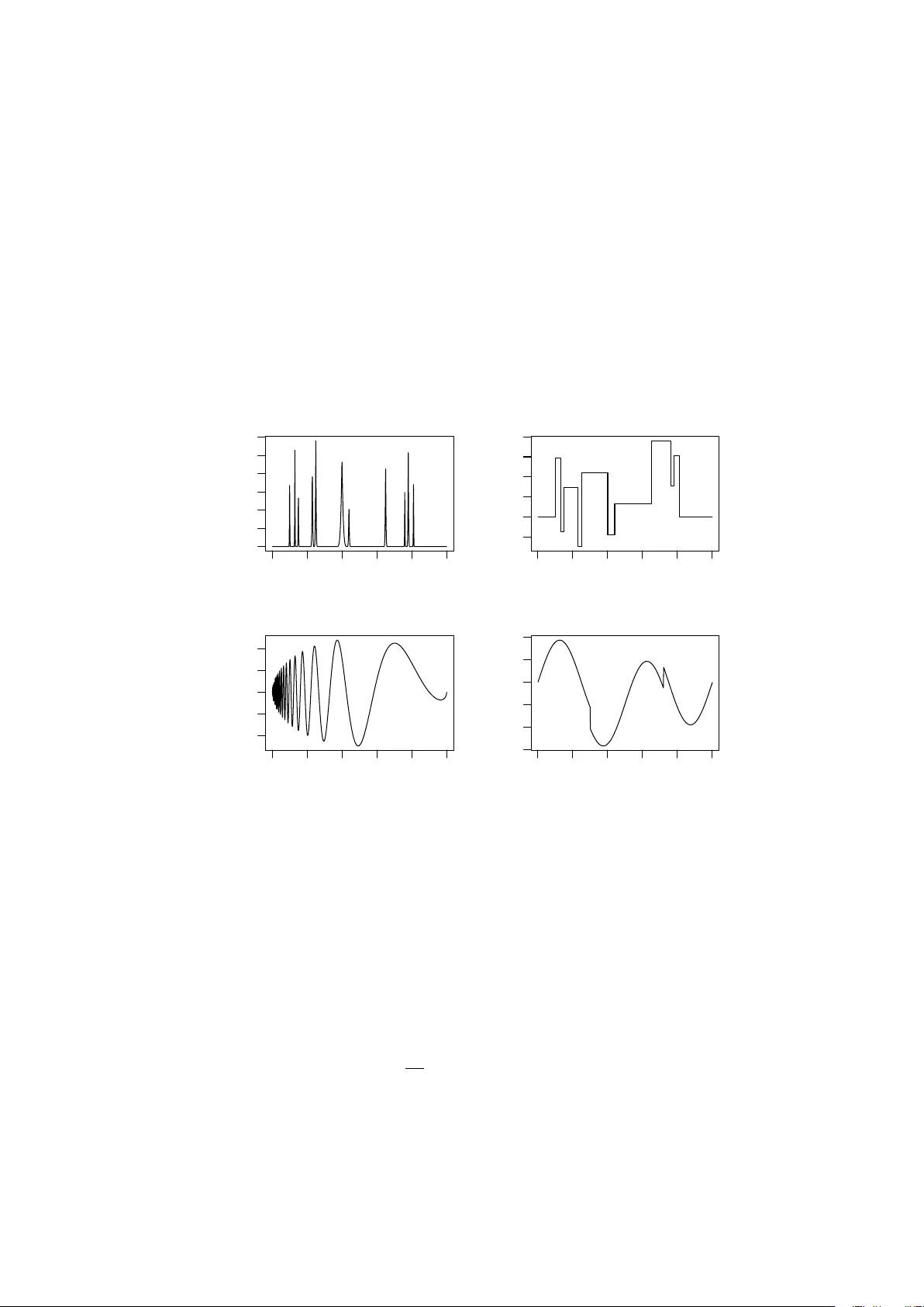
W a v elet-based estimation in aggregated functional data with p ositiv e and correlated errors Alex Ro drigo dos San tos Sousa ∗ , Jo˜ ao Victor Siqueira Ro drigues, Vitor Ribas P errone, and Raul Gomes Ro c ha Univ ersidade Estadual de Campinas (UNICAMP) Departamen t of Statistics, Brazil Abstract W e consider the statistical problem of estimating constituent curves from ob- serv ations of their aggregated curv es, referred to as aggregated functional data, in mo dels with strictly positive random errors under Gamma distribution and corre- lated errors under AR(1) and ARFIMA pro cesses. This problem arises in sev eral areas of knowledge, suc h as chemometrics, for example, when absorbance curves of the constituents of a giv en substance must b e estimated from its aggregated absorbance curve according to the Beer–Lambert law. In this sense, we prop ose Ba yesian w av elet-based metho ds to estimate the comp onen t functions under a functional data analysis approac h. This pro cedure has the adv antage of estimating curv es with important lo cal features, suc h as dis- con tinuities, p eaks, and oscillations, due to the expansion properties of functions in wa velet bases. W e further ev aluate the p erformance of the proposed method through computational simulations, as well as applications to real data. Keyw ords: aggregated data; gamma errors; long-memory errors; basis expansion. 1 In tro duction Across several scien tific domains, one encounters aggregated functional data gener- ated b y unkno wn comp onen t curv es. In spectroscopy , for instance, there is in terest ∗ asousa@unicamp.br 1 in estimating the individual mean absorbance curves of the constituents of a given substance from samples of aggregated absorbance curves of the substance itself. In this setting, b y the Beer–Lam b ert la w ( Brereton ( 2003 )), the o v erall absorbance is ex- pressed as a con v ex linear com bination of the absorbances of its constituen ts, with the com bination co efficien ts corresp onding to their concen trations in the samples. This problem is commonly referred to as calibration in chemometrics. Another example arises in mo deling the composition of electricity consumption in a giv en region, where the a verage load curve ov er a sp ecified time interv al is formed b y aggregating the consumption curves of individual consumers. F or further details on these examples, see Dias et al. ( 2009 ) and Dias et al. ( 2013 ). A v ariety of statistical m ethodologies hav e b een prop osed to estimate comp onen t curv es from aggregated observ ations. Man y of these approaches treat the data as m ultiv ariate because measuremen ts are collected at discrete time points. Thus, each sampled p oin t on the aggregated curve is considered as a v ariable with an asso ci- ated correlation structure. Principal Component Regression (PCR) by Cow e and McNicol ( 1985 ) and P artial Least Squares (PLS) by Sj¨ ostr¨ om et al. ( 1983 ) are usual m ultiv ariate methodologies for handling aggregated data. Bay esian approac hes and w av elet-based methods were also prop osed b y Brown et al. ( 1998a , b , 2001 ). Although successful in man y applications, suc h metho ds do not explicitly accoun t for the in trin- sic functional structure of the data, despite the fact that discretization arises merely from instrumental constraints, see Ramsay and Silv erman ( 1997 ) for an o verview of functional data analysis. In this direction, successful functional approac hes were first dev elop ed by Dias et al. ( 2009 , 2013 ), employing spline or B-spline expansions. Ho wev er, while spline expansions p erform w ell for smooth curv es, their p erformance deteriorates when the underlying comp onen t functions exhibit lo calized features such as discontin uities, sharp p eaks, or oscillatory b eha vior. In this sense, Sousa ( 2023 , 2024 ) proposed a w av elet-based approac h in functional data analysis to estimate com- p onen t functions in aggregated curv es. Ho wev er, b oth the m ultiv ariate and functional mo dels typically assume additive Gaussian errors, ev en though non-Gaussian noise is frequently observ ed in practice. F or example, Hupp ert ( 2016 ) and Sung et al. ( 2019 ) discuss the o ccurrence of non- Gaussian noise in sp ectroscopic measurements. Motiv ated by these limitations, w e prop ose the use of wa v elet-based metho ds to estimate individual mean comp onen t curv es from aggregated observ ations under models with t wo scenarios: (i) strictly 2 p ositiv e additive noise with Gamma distribution and (ii) correlated noise under an autoregressiv e or ARFIMA pro cess. In addition, w e prop ose to emplo y Bay esian w av elet shrink age rules based on a mixture prior consisting of a p oin t mass at zero and either a logistic distribution, as introduced by dos San tos Sousa ( 2022 ), to esti- mate wa v elet co efficien ts from empirical co efficien ts obtained via the discrete wa v elet transform (DWT) applied to the aggregated data. Additiv e strictly p ositiv e errors in the original model in tro duce substantial infer- en tial c hallenges. First, the independence prop erty is generally lost after the w av elet transform, that is, the transformed errors in the wa v elet domain are t ypically cor- related. Consequen tly , w av elet co efficien ts cannot be estimated indep enden tly , as is commonly done under Gaussian noise assumptions, but must instead b e inferred join tly from their p osterior distribution. This requirement t ypically necessitates com- putational strategies such as Marko v Chain Monte Carlo (MCMC) metho ds for sam- pling from the joint p osterior distribution. F urthermore, although the original errors are strictly p ositiv e, their wa v elet-domain representations correspond to linear com- binations and are not necessarily p ositiv e themselves, see Sousa and Garcia ( 2023 ). While sev eral statistical models with p ositiv e m ultiplicativ e noise hav e b een addressed via logarithmic transformations, models with positive additiv e noise are comparativ ely rare in the literature, despite their practical relev ance. See Radnosrati et al. ( 2020 ) for a dev elopment of estimation theory in mo dels with positive noise. On the other hand, correlated noises offer a different c hallenge. Although the decorrelation prop ert y of the DWT, the v ariabilities of the wa velet co efficien ts are differen t among resolution levels. Th us, the estimation pro cess requires a level- dep enden t approach that takes this difference into account, see Johnstone and Silver- man ( 1997 ). This pap er is organized as follows: Section 2 presents the statistical mo dels in- v olving aggregated curves considered in this w ork. The wa v elet-based estimation pro- cedures are describ ed in Section 3. Simulation studies to ev aluate the p erformance of the proposed methods are analyzed and discussed in Section 4. Real data applications are discussed in Section 5. Finally , Section 6 provides final considerations. 3 2 Statistical mo dels W e consider a function A ( t ) comp osed of a con vex linear combination of L ≥ 2 functions according to the model. A ( t ) = L X l =1 y l α l ( t ) + ϵ ( t ) , (1) where t ∈ R , α l ( t ) ∈ L 2 ( R ) = { f ( t ) : R R f 2 ( t ) dt < ∞} are unkno wn squared integrable functions, y l ∈ (0 , 1) and P L l =1 y l = 1 are known weigh ts, l = 1 , . . . , L and ϵ ( t ) is a random error pro cess. W e will call A ( t ) the aggregated function and α l ( t ) the comp onen t functions of the aggregation. In practice, we observe a sample of N aggregated curves at M = 2 J ( J ∈ N ) equally spaced locations according to the discrete v ersion of the mo del ( 1 ), A n ( t m ) = L X l =1 y nl α l ( t m ) + ϵ n ( t m ) , (2) n = 1 , . . . , N and m = 1 , . . . , M . The goal is to estimate the functions of the L comp onen ts α l ( t ) using observ ations ( t m , A n ( t m )) as data. This step is known as the calibration of the mo del ( 1 ). F unctional approaches to the calibration problem when ϵ ( t ) is a Gaussian pro cess w ere prop osed first b y Dias et al. ( 2009 ) and Dias et al. ( 2013 ) using splines ex- pansions of the comp onen t functions and recen tly b y Sousa ( 2023 ) and Sousa ( 2024 ) using w av elets represen tations of them. In this work, w e consider the wa v elet-based estimation of the component functions when the random errors are not Gaussian. Sp ecifically , tw o scenarios are considered on the distribution of the random errors: 1. ϵ n ( t m ) are p ositiv e, indep enden t and iden tically distributed (iid) and ha v e Gamma distribution with parameters a > 0 and b > 0, i.e, ϵ n ( t m ) ∼ Gamma( a, b ) and has probability density function giv en b y (w e dropp ed the indices for simplicit y), h ( ϵ ) = b a Γ( a ) ϵ a − 1 e − bϵ I ( ϵ > 0) , where Γ( · ) and I ( · ) are the Gamma and the indicator functions respectively . 2. ϵ n ( t m ) are correlated and follo w: (i) an autoregressive (AR) pro cess of order 1, i.e, ϵ n ( t m ) ∼ AR(1), ϵ i = ϕϵ i − 1 + η i , 4 where ϕ ∈ ( − 1 , 1) and η i are iid with Gaussian distribution, η i ∼ N(0 , σ 2 η ), σ η > 0 and (ii) an autoregressiv e fractionally in tegrated moving-a v erage pro cess (ARFIMA) of order (0 , d, 0), i.e, ϵ n ( t m ) ∼ ARFIMA(0 , d, 0), 0 < d < 0 . 5, (1 − B ) d ϵ = η i , where B is the backshift op erator, (1 − B ) d = P ∞ q =0 b q ( d ) B q with b q ( d ) = Γ( q − d ) / (Γ( q + 1)Γ( − d )) for q = 0 , 1 , . . . The scenarios hav e an imp ortan t impact on the estimation pro cedure under the w av elet approac h. If the random errors in the time domain are iid zero-mean Gaus- sian, then the random errors in the wa v elet domain remain iid zero-mean Gaussian with the same scale parameter. How ev er, if the errors are not Gaussian, the distribu- tion of their coun terparts in the w av elet domain is not preserv ed, see Neumann and v on Sac hs ( 1995 ). 3 Estimation pro cedures The estimation process starts by taking the data from the time domain to the w av elet domain. The discretized mo del ( 2 ) can b e written in matrix notation as A = αy + ϵ , (3) where A = ( A n ( t m )) M × N is the M × N matrix with the aggregated observ ations in whic h eac h column is a sample of M p oints, α = ( α l ( t m )) M × L is the M × L matrix with the unknown comp onen t functions, y = ( y nl ) L × N is the L × N matrix with the weigh ts of the comp onen t functions and ϵ = ( ϵ n ( t m )) M × N is the M × N matrix with the random errors. W e apply a Discrete W av elet T ransform (D WT) on the data, which can b e represen ted by the m ultiplication of an M × M orthogonal transformation matrix W on b oth sides of ( 3 ), obtaining the mo del in the wa v elet domain, D = Θ y + ε , (4) where D = W A is the M × N matrix with the empirical (observed) aggregated w av elet co efficien ts, Θ = W α is the M × L matrix with the unknown w av elet co- efficien ts of the comp onen t functions and ε = W ϵ is the M × N matrix with the 5 random errors in the wa v elet domain. T o remo ve the noise in ( 4 ), w e apply a wa v elet shrink age rule δ ( · ) in the matrix with the empirical co efficients D and estimate Θ b y ˆ Θ = δ ( D ) y ′ ( y y ′ ) − 1 . (5) Finally , the matrix α is estimated by applying the In verse Discrete W av elet T ransform (ID WT), represen ted by the transpose matrix of W , ˆ α = W ′ ˆ Θ . See Sousa ( 2024 ) for more details. The distribution of random errors in ( 2 ) affects the w av elet shrink age rule to b e applied to the empirical w av elet co efficien ts in ( 5 ). The next subsections pro vide details of the wa v elet shrink age pro cedure under the tw o scenarios of errors considered. 3.1 Application of w a velet shrink age under pos itive (Gamma) ran- dom error Under the scenario of iid positive random errors with Gamma distribution in the mo del ( 2 ), we hav e that the probability densit y function of ε = W ϵ is giv en by f ( ε ) =  b a Γ( a )  n exp ( − b n X i =1 n X k =1 w ki ε k ) n Y i =1 n X k =1 w ki ε k ! a − 1 n Y i =1 I (0 , ∞ ) n X k =1 w ki ε k ! . Then, doing ε = d − θ , the likelihoo d function is L ( θ | d ) =  b a Γ( a )  n exp ( − b n X i =1 n X k =1 w ki ( d k − θ k ) ) n Y i =1 n X k =1 w ki ( d k − θ k ) ! a − 1 × × n Y i =1 I (0 , ∞ ) n X k =1 w ki ( d k − θ k ) ! . (6) W e adopt the mixture of a p oin t mass function at zero and the cen tered-around- zero logistic distribution with scale parameter τ > 0 as prior distribution to a single w av elet co efficien t, as prop osed by dos Santos Sousa ( 2022 ). Th us, the join t prior distribution of θ is π ( θ ) = n Y i =1 [ pδ 0 ( θ i ) + (1 − p ) g ( θ i ; τ ) , (7) where p ∈ (0 , 1), δ 0 ( · ) is the p oin t mass function at zero and g ( · ; τ ) is the logistic probabilit y density function cen tered at zero. Considering ( 6 ) and ( 7 ), the asso ciated 6 p osterior distribution is π ( θ | d ) ∝ π ( θ ) L ( θ | d ) ∝    n Y i =1    pδ 0 ( θ i ) + (1 − p ) exp n − θ i τ o τ  1 + exp n − θ i τ o 2       exp ( − b n X i =1 n X k =1 w ki ( d k − θ k ) ) × × n Y i =1 n X k =1 w ki ( d k − θ k ) ! a − 1 n Y i =1 I (0 , ∞ ) n X k =1 w ki ( d k − θ k ) ! . (8) Note that, although the error ϵ in the time domain is indep endent, after applying the D WT the error in the w av elet domain ε is no longer independent, a fact due to the loss of normality . Therefore, the shrink age rule must b e applied to the vector of co efficien ts, and it is no longer p ossible to apply it co efficien t by co efficien t. In Ba yesian settings, the shrink age rule is computed through the p osterior ex- p ectation, that is, δ ( d ) = E ( θ | d ). Ho w ever, in this case this is not analytically tractable, requiring the use of Marko v Chain Monte Carlo (MCMC) methods. The idea is to generate K samples from the p osterior distribution ( 8 ) and approximate ˆ θ i b y the av erage of the generated samples, that is, ˆ θ i = δ i ( d ) ≈ 1 K K X k =1 θ ki . It is w orth noting that, when using this metho d, it is common to employ a burn-in p eriod, in which the initial part of the chain is discarded to reduce dep endence on the starting point, and thinning, whic h consists of retaining only ev ery j -th sample gener- ated by the c hain in order to reduce the autocorrelation among successiv e iterations. See Rob ert et al. ( 2004 ) for more details ab out MCMC methods. T o approximate this exp ectation, we employ the Algorithm 1 , the Robust Adap- tiv e Metropolis (RAM) algorithm prop osed by Vihola ( 2012 ). This method relies on a lo wer triangular matrix S k with p ositiv e diagonal elemen ts, which is up dated at eac h iteration. Moreov er, { η l } l ≥ 1 ⊂ (0 , 1] denotes a sequence that decays to zero, and γ ∈ (0 , 1) represen ts the target av erage acceptance rate. T o elicite the h yp erparameters τ and p in ( 7 ), we follow the prop osals of dos San tos Sousa ( 2022 ) and Angelini and Vidako vic ( 2004 ) resp ectiv ely , i.e, τ should b e c hosen suc h that 0 < τ ≤ 10 and p = p ( j ) = 1 − 1 ( j − J 0 + 1) h , (9) 7 where J 0 ≤ j ≤ J − 1, J 0 is the primary resolution level, J is the n umber of resolution lev els, J = log 2 ( n ) and h > 0. They also suggested that in the absence of additional information, h = 2 can b e adopted. Algorithm 1: Robust Adaptiv e Metrop olis (RAM). Input: θ 1 , S 1 , { η l } l ≥ 1 ⊂ (0 , 1], γ ∈ (0 , 1), and K (num b er of iterations). Output: Samples θ 1 , . . . , θ K from π ( θ | d ). k ← 2 Generate θ ∗ k = θ k − 1 + S k − 1 U k , where U k ∼ N n ( 0 , I ) Set θ k = θ ∗ k with probability γ k , otherwise set θ k = θ k − 1 , where γ k = min  1 , π ( θ ∗ k ) π ( θ k − 1 )  Compute the lo wer triangular matrix S k with p ositiv e diagonal elements satisfying S k S ′ k = S k − 1  I + η k ( γ k − γ ) U k U ′ k ∥ U k ∥ 2  S ′ k − 1 k ← k + 1 and, if k ≤ K , return to Step 2 3.2 Application of w av elet shrink age under correlated random error In the second scenario, the errors in ( 2 ) are assumed to be correlated, follo wing AR(1) and ARFIMA(0 , d, 0) pro cesses. Due to the decorrelation prop ert y of the D WT, the shrink age rule can b e applied individually to each empirical co efficient. Ho wev er, applying the rule inv olv es estimating the stand ard deviation of the empirical co efficien ts at each resolution level, i.e, the shrink age rule m ust b e lev el-dep enden t, see Johnstone and Silv erman ( 1997 ). In this sense, w e apply the Ba y esian approach of Sousa and Zev allos ( 2025 ) to the context of aggregated functional data. The shrink age rule to b e applied on a single empirical w av elet coefficient d at the resolution lev el j is δ j ( d ) = (1 − p ) R R ( ˆ σ j u + d ) g ( ˆ σ j u + d ; τ ) ϕ ( u ) du p ˆ σ j ϕ  d ˆ σ j  + (1 − p ) R R g ( ˆ σ j u + d ; τ ) ϕ ( u ) du , where ˆ σ j = ˆ σ ( j ) = median { | d j,k | : k = 0 , . . . , 2 j } 0 . 6745 . 8 4 Sim ulation studies W e conducted sim ulation studies to ev aluate the performance of the prop osed meth- o ds. T o do so, we adopted the so-called Donoho and Johnstone (DJ) test functions as underlying comp onen t functions in ( 1 ). These functions called Bumps, Blo cks, Doppler and Hea visine ha v e in teresting lo cal features to b e estimated suc h as p eaks, discon tinuities and oscillations, see Donoho and Johnstone ( 1994 ) for more details. Figure 1 sho ws the plots of the DJ-test functions. 0.0 0.2 0.4 0.6 0.8 1.0 0 10 20 30 40 50 60 x Bumps 0.0 0.2 0.4 0.6 0.8 1.0 −5 0 5 10 15 20 x Blocks 0.0 0.2 0.4 0.6 0.8 1.0 −10 −5 0 5 10 x Doppler 0.0 0.2 0.4 0.6 0.8 1.0 −15 −10 −5 0 5 10 x Heavisine Figure 1: Donoho and Johnstone test functions. In b oth positive and correlated errors scenarios, w e generated the data according to the mo del ( 2 ) for sp ecific v alues of sample size N , num b er of points M and n umber of comp onen t functions L . F urther, the v ariance of the error was also obtained according to sp ecific v alues of signal-to-noise ratio (SNR). As p erformance measure, for each replication r and comp onen t function α ( · ), we calculated the mean squared error (MSE), MSE r = 1 M M X i =1  ˆ α ( r ) ( t i ) − α ( t i )  2 , where ˆ α ( r ) ( t i ) denotes the estimate of α ( t i ), for i = 1 , . . . , M . Then, we finally 9 obtained the a veraged mean squared error (AMSE) AMSE = 1 R R X r =1 MSE r , where R is the n umber of replications. In the next tw o subsections we present more details and the results for each error scenario. 4.1 Results for p ositiv e (Gamma) error In the mo del ( 2 ) under iid gamma errors, we adopted N = 50 curves, M = 32 and 64 equally spaced p oin ts, L = 2 (Bumps and Doppler as underlying comp onent functions) and 4 (all the DJ test functions as underlying comp onen t functions) and SNR = 3 and 7. F urther, we chose a fixed p = 0 . 75 and τ = 5 as h yp erparameters of the prior distribution ( 7 ). W e run R = 400 replications and the size of the generated c hains of the Algorithm 1 in eac h replication w as 50,000. T able 1 presen ts the AMSE and the standard deviation of the MSE of the prop osed metho d for each comp onen t function, M , L and SNR. The results indicate a clear deterioration in the method’s performance as the n um b er of comp onen t curv es L to be estimated increases. F urthermore, the error w as consisten tly smaller in scenarios with higher SNR, as expected, since such settings inv olv e lo wer noise levels and therefore pro vide more fav orable signal reco very conditions. In addition, T able 2 presents the AMSE and the standard deviation of the prop osed metho d but for the aggregated curv es A ( · ) and Figure 2 sho ws the boxplots of the MSE for L = 2 comp onen t functions. 10 T able 1: AMSE (standard deviation) of the prop osed metho d for each comp onen t function under gamma noise. F unction SNR M L = 2 L = 4 Bumps 3 32 0.925 (0.279) 4.235 (1.478) 64 1.637 (0.302) 4.878 (1.279) 7 32 0.121 (0.038) 0.663 (0.212) 64 0.652 (0.17) 1.434 (0.459) Doppler 3 32 0.877 (0.282) 4.125 (1.504) 64 1.616 (0.301) 4.814 (1.333) 7 32 0.121 (0.038) 0.645 (0.245) 64 0.659 (0.163) 1.389 (0.448) Blo c ks 3 32 - 4.149 (1.463) 64 - 4.801 (1.309) 7 32 - 0.639 (0.231) 64 - 1.38 (0.525) Hea visine 3 32 - 4.225 (1.617) 64 - 4.847 (1.281) 7 32 - 0.64 (0.205) 64 - 1.36 (0.466) 11 T able 2: AMSE (standard deviation) of the prop osed method under gamma noise. SNR M L = 2 L = 4 3 32 0.901 (0.195) 4.183 (0.843) 64 1.626 (0.185) 4.835 (0.689) 7 32 0.121 (0.031) 0.647 (0.127) 64 0.655 (0.076) 1.391 (0.173) 32 64 32 64 0.0 0.5 1.0 1.5 2.0 2.5 M AMSE snr = 3 snr = 7 Figure 2: Boxplots of the MSE of the prop osed metho d in the model under iid gamma errors for L = 2 comp onen t functions (Bumps and Doppler). The MSE is related to the estimation of the aggregated curve. 4.2 Results for correlated (AR and ARFIMA) errors In the sim ulation of the model under correlated errors, we considered three n umbers of equally spaced p oin ts in each curve, M = 512 , 1024 and 2048, three signal-to-noise ratio v alues, SNR = 3 , 5 and 7, and a sample size N = 100. The error structures analyzed included AR(1) pro cesses, with parameters ϕ = 0 . 25 and 0 . 5 as w ell as 12 ARFIMA(0, d , 0) pro cesses, with parameters d = 0 . 2 and 0 . 4, allowing the ev aluation of b oth short- and long-range dependence. Accordingly , four simulation studies were conducted, considering different com- binations of the test functions and R = 200 replications for each scenario. In the first sim ulation, the Blocks and Bumps functions ( L = 2) w ere used, and the results are presented in T able 3 . The second sim ulation includes the Doppler and Hea visine functions ( L = 2 to o), with results shown in T able 4 . The third sim ulation considers the Blo c ks, Bumps, and Heavisine functions ( L = 3), with results presen ted in T able 5 . Finally , the fourth simulation incorp orates all the DJ test functions ( L = 4), with results rep orted in T able 6 . T able 3: AMSE (standard deviation) of the prop osed metho d in the mo del under iid normal and correlated errors for L = 2 comp onen t functions (Bumps and Blo c ks). The AMSE is related to the estimation of the aggregated curve. n Error structure SNR = 3 SNR = 5 SNR = 7 512 Normal iid 1.8915(0.0611) 1.3931(0.0510) 1.1544(0.0345) 512 AR(1) - ϕ = 0 . 25 2.1197(0.0711) 2.0309(0.0485) 1.9784(0.0409) 512 AR(1) - ϕ = 0 . 5 2.2401(0.0804) 2.1276(0.0705) 2.0541(0.0590) 512 AR(1) - ϕ = 0 . 9 2.5710(0.1586) 2.4646(0.1386) 2.3776(0.1281) 512 ARFIMA(0,0.2,0) 2.3302(0.1328) 2.2050(0.1004) 2.1276(0.0917) 512 ARFIMA(0,0.4,0) 2.3624(0.2976) 2.2339(0.2126) 2.1899(0.1824) 1024 Normal iid 1.5072(0.0473) 1.1258(0.0287) 0.9419(0.0243) 1024 AR(1) - ϕ = 0 . 25 2.1078(0.0468) 2.0381(0.0320) 1.9912(0.0287) 1024 AR(1) - ϕ = 0 . 5 2.1957(0.0697) 2.1103(0.0445) 2.0624(0.0370) 1024 AR(1) - ϕ = 0 . 9 2.5463(0.1216) 2.4301(0.1112) 2.3487(0.1008) 1024 ARFIMA(0,0.2,0) 2.3370(0.1091) 2.2175(0.0860) 2.1460(0.0719) 1024 ARFIMA(0,0.4,0) 2.4114(0.2561) 2.3379(0.2049) 2.2768(0.1654) 2048 Normal iid 1.2015(0.0278) 0.9158(0.0212) 0.7475(0.0183) 2048 AR(1) - ϕ = 0 . 25 2.0777(0.0293) 2.0321(0.0245) 1.9988(0.0206) 2048 AR(1) - ϕ = 0 . 5 2.1394(0.0420) 2.0830(0.0296) 2.0495(0.0251) 2048 AR(1) - ϕ = 0 . 9 2.4511(0.1143) 2.3397(0.0920) 2.2742(0.0746) 2048 ARFIMA(0,0.2,0) 2.2915(0.0866) 2.2027(0.0729) 2.1407(0.0603) 2048 ARFIMA(0,0.4,0) 2.4124(0.2431) 2.3610(0.1934) 2.3134(0.1645) 13 T able 4: AMSE (standard deviation) of the prop osed metho d in the mo del under iid normal and correlated errors for L = 2 comp onen t functions (Doppler and Hea visine). The AMSE is related to the estimation of the aggregated curve. n Error structure SNR = 3 SNR = 5 SNR = 7 512 Normal iid 1.1974(0.0755) 0.7514(0.0412) 0.5369(0.0332) 512 AR(1) - ϕ = 0 . 25 4.5979(0.0308) 4.6023(0.0326) 4.6117(0.0284) 512 AR(1) - ϕ = 0 . 5 4.5975(0.0354) 4.6000(0.0319) 4.6040(0.0338) 512 AR(1) = ϕ = 0 . 9 4.6431(0.0562) 4.6319(0.0499) 4.6118(0.0445) 512 ARFIMA(0,0.2,0) 4.5889(0.0462) 4.5882(0.0430) 4.5888(0.0368) 512 ARFIMA(0,0.4,0) 4.5869(0.1581) 4.5737(0.1249) 4.5557(0.0985) 1024 Normal iid 0.8586(0.0467) 0.5131(0.0301) 0.3440(0.0244) 1024 AR(1) - ϕ = 0 . 25 4.6526(0.0301) 4.6772(0.0274) 4.6924(0.023) 1024 AR(1) - ϕ = 0 . 5 4.6390(0.0333) 4.6529(0.0299) 4.6648(0.0279) 1024 AR(1) - ϕ = 0 . 9 4.6463(0.0428) 4.6372(0.0423) 4.6359(0.0359) 1024 ARFIMA(0,0.2,0) 4.6177(0.0436) 4.6228(0.0358) 4.6276(0.0316) 1024 ARFIMA(0,0.4,0) 4.6136(0.1488) 4.5949(0.1087) 4.5903(0.0947) 2048 Normal iid 0.5810(0.0372) 0.3113(0.0194) 0.2140(0.0136) 2048 AR(1) - ϕ = 0 . 25 4.7036(0.0231) 4.7297(0.0185) 4.7407(0.0157) 2048 AR(1) - ϕ = 0 . 5 4.6738(0.0272) 4.7048(0.0261) 4.7166(0.0206) 2048 AR(1) - ϕ = 0 . 9 4.6492(0.0405) 4.6468(0.0375) 4.6509(0.0347) 2048 ARFIMA(0,0.2,0) 4.6346(0.0409) 4.6434(0.0347) 4.6563(0.0335) 2048 ARFIMA(0,0.4,0) 4.6032(0.1253) 4.5847(0.1112) 4.5888(0.0900) 14 T able 5: AMSE (standard deviation) of the prop osed metho d in the mo del under iid normal and correlated errors for L = 3 component functions (Bumps, Blo c ks and Hea visine). The AMSE is related to the estimation of the aggregated curv e. n Error structure SNR = 3 SNR = 5 SNR = 7 512 Normal iid 2.2510(0.1452) 1.5821(0.0832) 1.2625(0.0743) 512 AR(1) - ϕ = 0 . 25 4.4710(0.0957) 4.3859(0.0706) 4.3385(0.0670) 512 AR(1) - ϕ = 0 . 5 4.5650(0.1131) 4.4768(0.0928) 4.4242(0.0827) 512 AR(1) - ϕ = 0 . 9 4.8098(0.1931) 4.7403(0.1655) 4.6976(0.1528) 512 ARFIMA(0,0.2,0) 4.6186(0.1499) 4.5185(0.1193) 4.4661(0.1051) 512 ARFIMA(0,0.4,0) 4.6623(0.4457) 4.5464(0.2921) 4.5234(0.2733) 1024 Normal iid 1.7413(0.0943) 1.2384(0.0674) 0.9829(0.0528) 1024 AR(1) - ϕ = 0 . 25 4.4788(0.0750) 4.4154(0.0651) 4.3840(0.0584) 1024 AR(1) - ϕ = 0 . 5 4.5555(0.0904) 4.4862(0.0743) 4.4471(0.0673) 1024 AR(1) - ϕ = 0 . 9 4.8193(0.1539) 4.7320(0.1389) 4.6750(0.1143) 1024 ARFIMA(0,0.2,0) 4.6416(0.1307) 4.5708(0.1181) 4.5146(0.0927) 1024 ARFIMA(0,0.4,0) 4.6817(0.3863) 4.6167(0.2983) 4.5860(0.2627) 2048 Normal iid 1.3434(0.0686) 0.9480(0.0472) 0.7415(0.0399) 2048 AR(1) - ϕ = 0 . 25 4.4659(0.0595) 4.4305(0.0578) 4.4035(0.0499) 2048 AR(1) - ϕ = 0 . 5 4.5275(0.0726) 4.4693(0.0615) 4.4441(0.0564) 2048 AR(1) - ϕ = 0 . 9 4.7647(0.1244) 4.6934(0.1090) 4.6344(0.1066) 2048 ARFIMA(0,0.2,0) 4.6310(0.1142) 4.5605(0.1038) 4.5163(0.0836) 2048 ARFIMA(0,0.4,0) 4.6724(0.3380) 4.6314(0.2855) 4.6100(0.2228) 15 T able 6: AMSE (standard deviation) of the prop osed metho d in the mo del under iid normal and correlated errors for L = 4 comp onen t functions (all the DJ test functions). The AMSE is related to the estimation of the aggregated curve. n Error structure SNR = 3 SNR = 5 SNR = 7 512 Normal iid 1.9290(0.1516) 1.3500(0.1011) 1.0787(0.0759) 512 AR(1) - ϕ = 0 . 25 3.4031(0.0867) 3.3381(0.0779) 3.2957(0.0702) 512 AR(1) - ϕ = 0 . 5 3.4852(0.1100) 3.4130(0.0971) 3.3669(0.0775) 512 AR(1) - ϕ = 0 . 9 3.6679(0.1802) 3.6088(0.1558) 3.5647(0.1421) 512 ARFIMA(0,0.2,0) 3.5254(0.1504) 3.4467(0.1249) 3.4076(0.1127) 512 ARFIMA(0,0.4,0) 3.6991(0.5873) 3.5478(0.3846) 3.4857(0.3324) 1024 Normal iid 1.4856(0.1084) 1.0679(0.0744) 0.8546(0.0590) 1024 AR(1) - ϕ = 0 . 25 3.3980(0.0730) 3.3593(0.0625) 3.3341(0.0610) 1024 AR(1) - ϕ = 0 . 5 3.4713(0.0911) 3.4123(0.0772) 3.3798(0.0666) 1024 AR(1) - ϕ = 0 . 9 3.6692(0.1340) 3.6028(0.1294) 3.5662(0.1133) 1024 ARFIMA(0,0.2,0) 3.5424(0.1278) 3.4800(0.1124) 3.4401(0.0993) 1024 ARFIMA(0,0.4,0) 3.6688(0.5341) 3.5791(0.3675) 3.5415(0.3052) 2048 Normal iid 1.1614(0.0735) 0.8263(0.0533) 0.6563(0.0420) 2048 AR(1) - ϕ = 0 . 25 3.3893(0.0580) 3.3692(0.0528) 3.3474(0.0510) 2048 AR(1) - ϕ = 0 . 5 3.4388(0.0715) 3.4049(0.0645) 3.3797(0.0588) 2048 AR(1) - ϕ = 0 . 9 3.6304(0.1256) 3.5619(0.1007) 3.5335(0.0919) 2048 ARFIMA(0,0.2,0) 3.5260(0.1066) 3.4747(0.0993) 3.4494(0.0859) 2048 ARFIMA(0,0.4,0) 3.6672(0.4354) 3.5774(0.3239) 3.5370(0.2729) In general, it can be observ ed that the mo del is reasonably robust to b oth short- and long-memory error structures. In general, the mean MSE in the most extreme scenario is b et w een three and four times larger than in the ideal case; ho wev er, in absolute numerical terms, this difference remains small. Moreo ver, in Johnstone and Silverman ( 1997 ), not only was a pro cedure prop osed for estimating the v ariance, but also a thresholding strategy , namely the univ ersal threshold metho d. In order to compare this approac h with the Bay esian method, an additional simulation study was conducted under the most challenging setting: all four test functions aggregated and errors following an ARFIMA(0, 0.4, 0) pro cess. T able 7 presents the comparison b etw een the estimation metho ds, again based on 16 200 replications for each scenario. F rom the table, it can b e seen that the differences b et w een the approaches are not substan tial; nev ertheless, the Ba yesian estimator generally yields sligh tly better results than the univ ersal thresholding metho d. T able 7: AMSE (standard deviation) of the prop osed metho d and the Johnstone and Silv erman metho d in the model under ARFIMA(0, 0.4, 0) errors for L = 4 comp onen t functions (all the DJ test functions). The AMSE is related to the estimation of the aggregated curve. n SNR Ba y esian Johnstone e Silverman 512 3 3.6632(0.5538) 3.6705(0.5135) 512 5 3.5710(0.4164) 3.6184(0.3984) 512 7 3.4881(0.3236) 3.5664(0.3137) 1024 3 3.6906(0.5225) 3.6952(0.4794) 1024 5 3.5929(0.3683) 3.6360(0.3545) 1024 7 3.5159(0.2863) 3.5778(0.2839) 2048 3 3.7140(0.4933) 3.7239(0.4669) 2048 5 3.5533(0.3115) 3.5890(0.2983) 2048 7 3.5268(0.2627) 3.5756(0.2515) 5 Real data illustrations 6 Final considerations Within the framew ork of the Aggregated F unctional Data Analysis paradigm, w a velet basis expansions were emplo y ed to estimate the mean curves of component func- tions under p ositiv e and correlated error models. T o this end, b oth classical and Ba yesian approac hes were inv estigated, along with the necessary computational as- p ects required for implemen tation, including the Random W alk Metrop olis (RAM) algorithm. In this sense, it w as possible to dev elop a mo del for aggregated curv es under a p os- itiv e error structure, specifically , the Gamma distribution—which remains relativ ely unexplored in the literature and therefore presen ts clear publication p oten tial. sim u- lation studies were conducted to examine the behavior of the prop osed method across a wide range of scenarios, allowing for a comprehensive assessmen t of its empirical 17 p erformance. Additionally , we conducted an extensiv e sim ulation study to assess the robustness of the wa v elet-based metho d under violations of the indep endence assumption for the errors, considering both short and long-memory dep endence structures. The results indicate that, although the presence of correlation among the errors increases the mean squared error relativ e to the ideal indep enden t-error scenario, the estimator’s o verall p erformance remains stable and satisfactory across most of the configurations examined. F urthermore, the comparison b et ween the Ba y esian shrink age rule and the univ ersal thresholding metho d of Johnstone and Silverman suggests a sligh t adv an tage in fa vor of the Ba yesian estimator, particularly under more c hallenging dep endence settings. Ac kno wledgmen ts A.R.S.S, V.R.P and R.G.R w ere financed by Programa de Incentiv o a No vos Do centes (PIND) da Universidade Estadual de Campinas, grant 3376/23 and J.V.S.R w as fi- nanced b y F unda¸ c˜ ao de Amparo ` a P esquisa do Estado de S˜ ao Paulo (F APESP), gran t 11042/0. References C. Angelini and B. Vidako vic. Gama-minimax w a velet shrink age: a robust incorp o- ration of information about energy of a signal in denoising applications. Stat Sin , 14(1):103–125, 2004. Ric hard G Brereton. Chemometrics: data analysis for the lab or atory and chemic al plant . John Wiley & Sons, 2003. Philip J Bro wn, Marina V ann ucci, and T om F earn. Ba yesian w av elength selection in m ulticomp onen t analysis. Journal of Chemometrics: A Journal of the Chemomet- rics So ciety , 12(3):173–182, 1998a. Philip J Brown, Marina V annucci, and T om F earn. Multiv ariate bay esian v ariable se- lection and prediction. Journal of the R oyal Statistic al So ciety: Series B (Statistic al Metho dolo gy) , 60(3):627–641, 1998b. 18 Philip J Bro wn, T om F earn, and Marina V ann ucci. Ba yesian wa v elet regression on curv es with application to a spectroscopic calibration problem. Journal of the A meric an Statistic al Asso ciation , 96(454):398–408, 2001. Ian A Cow e and James W McNicol. The use of principal components in the analysis of near-infrared spectra. Applie d sp e ctr osc opy , 39(2):257–266, 1985. R. Dias, N. L. Garcia, and A. Martarelli. Non-parametric estimation for aggregated functional data for electric load monitoring. Envir onmetrics , 20(2):111–130, 2009. R. Dias, N. L. Garcia, and A. Sc hmidt. A hierarc hical model for aggregated functional data. T e chnometrics , 55(13):321–334, 2013. D.L. Donoho and I.M. Johnstone. Ideal spatial adaptation b y wa v elet shrink age. Biometrika , 81(1):425–455, 1994. Alex Ro drigo dos Santos Sousa. Ba yesian w av elet shrink age with logistic prior. Com- munic ations in Statistics-Simulation and Computation , 51(8):4700–4714, 2022. Theo dore J Hupp ert. Commentary on the statistical prop erties of noise and its im- plication on general linear mo dels in functional near-infrared sp ectroscopy . Neu- r ophotonics , 3(1):010401–010401, 2016. I.M. Johnstone and B.W. Silverman. W a v elet threshold estimators for data with correlated noise. Journal of the R oyal Statistic al So ciety B , 59(2):319–351, 1997. M.H. Neumann and R. v on Sac hs. Wavelet Thr esholding: Beyond the Gaussian I.I.D. Situation. In: Antoniadis, A., Opp enheim, G. (e ds) Wavelets and Statistics. L e ctur e Notes in Statistics . Springer, New Y ork, NY, 1995. Kamiar Radnosrati, Gustaf Hendeb y , and F redrik Gustafsson. Exploring positive noise in estimation theory . IEEE T r ansactions on Signal Pr o c essing , 68:3590–3602, 2020. James O Ramsa y and Bernard W Silv erman. F unctional data analysis . Springer, 1997. Christian P Rob ert, George Casella, and George Casella. Monte Carlo statistic al metho ds , volume 2. Springer, 2004. 19 Mic hael Sj¨ ostr¨ om, Sv ante W old, W alter Lindb erg, Jan- ˚ Ak e P ersson, and Harald Martens. A multiv ariate calibration problem in analytical c hemistry solved b y par- tial least-squares mo dels in latent v ariables. Analytic a Chimic a A cta , 150:61–70, 1983. A.R.S. Sousa. Sim ulation studies to compare bay esian w a velet shrink age metho ds in aggregated functional data. CSAM , 30(1):311–330, 2023. A.R.S. Sousa. A w a velet-based method in aggregated functional data analysis. Monte Carlo Metho ds and Applic ations , 30(1):19–30, 2024. A.R.S. Sousa and N.L. Garcia. W a velet shrink age in nonparametric regression models with p ositiv e noise. Journal of Statistic al Computation and Simulation , 93(17): 3011–3033, 2023. A.R.S. Sousa and M. Zev allos. On bay esian wa v elet shrink age estimation of nonpara- metric regression mo dels with stationary correlated noise. Stat Comput , 35(85), 2025. Y oungkyu Sung, F ´ elix Beaudoin, Leigh M Norris, F ei Y an, David K Kim, Jac k Y Qiu, Uwe von L ¨ upke, Jonilyn L Y o der, T erry P Orlando, Simon Gusta vsson, et al. Non-gaussian noise spectroscopy with a superconducting qubit sensor. Natur e c om- munic ations , 10(1):3715, 2019. Matti Vihola. Robust adaptiv e metrop olis algorithm with co erced acceptance rate. Statistics and c omputing , 22(5):997–1008, 2012. 20