Conformal Selective Prediction with General Risk Control

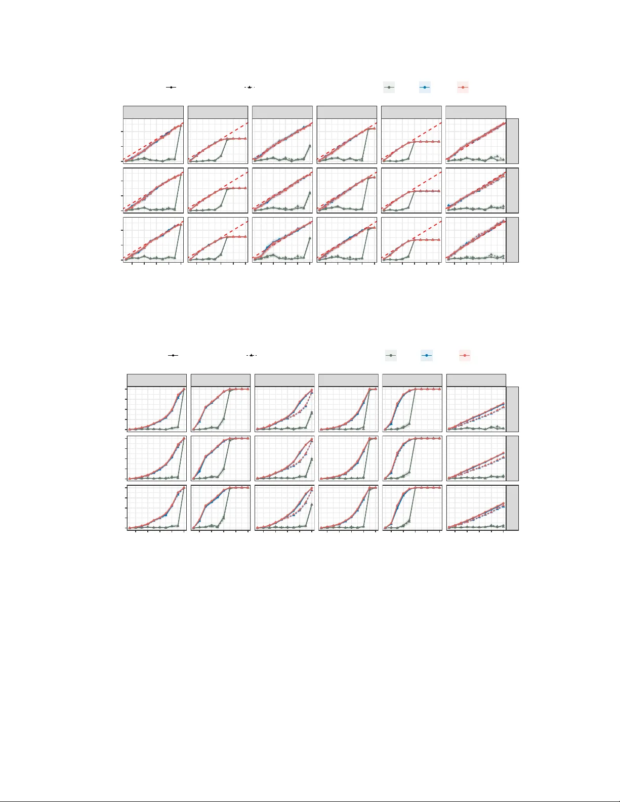
Conformal Selectiv e Prediction with General Risk Con trol Tian Bai 1 and Ying Jin 2 1 Departmen t of Statistics, Stanford Universit y 2 Departmen t of Statistics and Data Science, Universit y of P ennsylv ania Abstract In deplo ying artiﬁcial intelligence (AI) models, selective prediction oﬀers the option to abstain from making a prediction when uncertain ab out model qualit y . T o fulﬁll its promise, it is crucial to enforce strict and precise error con trol ov er cases where the model is trusted. W e propose Selectiv e Conformal Risk control with E-v alues (SCoRE), a new framework for deriving such decisions for an y trained mo del and any user-deﬁned, b ounded and contin uously-v alued risk. SCoRE oﬀers t wo types of guarantees on the risk among “p ositiv e” cases in whic h the system opts to trust the mo del. Built upon conformal inference and hypothesis testing ideas, SCoRE ﬁrst constructs a class of (generalized) e-v alues, which are non-negative random v ariables whose pro duct with the unknown risk has exp ectation no greater than one. Suc h a prop ert y is ensured b y data exc hangeability without requiring an y modeling assumptions. P assing these e-v alues on to h yp othesis testing procedures, w e yield the binary trust decisions with ﬁnite-sample error con trol. SCoRE a voids the need of uniform concen tration, and can be readily extended to settings with distribution shifts. W e ev aluate the proposed methods with sim ulations and demonstrate their eﬃcacy through applications to error management in drug disco very , health risk prediction, and large language mo dels. Keywor ds: Selectiv e prediction; Conformal inference; Hyp othesis testing; Multiple testing; T rust worth y AI. 1 In tro duction Limiting errors when deploying AI models is an indisp ensable comp onen t of their life cycle ( Wiens et al. , 2019 ; Kompa et al. , 2021 ). As mo del prediction errors are inevitable—arising from inadequate mo deling, sampling uncertain ty , and randomness in training—p ost-training mechanisms that manage errors at deplo yment are esp ecially important. A prominen t approach is to deploy a model with an abstention (or r eje ction ) option: a mo del is used only when it appears reliable and is withheld otherwise ( Cho w , 2009 ; El-Y aniv et al. , 2010 ). This paradigm, often called sele ctive pr e diction , aims to con trol errors precisely among the predictions we c ho ose to deplo y while maintaining high co verage, i.e., deplo ying as often as p ossible ( Geifman and El-Y aniv , 2017 ). This leads to the general question: Given a black-b ox mo del f , lab ele d data { ( X i , Y i ) } n i =1 and a new instanc e X n +1 , c an we derive a trust de cision ψ n +1 ∈ { 0 , 1 } that c ontr ols an unknown risk L n +1 among those with ψ n +1 = 1 ? Most prior work addresses this problem for classiﬁers f with binary risks L n +1 ∈ { 0 , 1 } , typically oﬀering either asymptotic control of a selective error rate or ﬁnite-sample b ound based on uniform concentration of empirical classiﬁcation errors. Recent extensions of conformal prediction provide ﬁnite-sample, distribution- free guarantees for selectiv e tasks with binary risks ( V ovk et al. , 2005 ; Jin and Cand` es , 2023b , a ), and ha ve b een used to identify trust worth y AI outputs in applications such as comp ound screening ( Bai et al. , 2025 ),large language mo dels ( Gui et al. , 2024 ; Jung et al. , 2024 ), and medical foundation mo dels ( Jin et al. , 2026 ). Ho wev er, many high-stakes applications demand control of c ontinuously-value d risks, where a principled and p ow erful “trust” mec hanism remains underdev elop ed: 1 Unknown affinity 𝑌 !"# Development cost 𝐿 !"# AI model SCoRE Ye s No No enough confidence! New drug candidate SDR guarantee: Avg false-lead cost among deployed ≤ 𝛼 ? X 0 2 4 6 8 −7 −6 −5 −4 Drug binding affinity (unknown) Follo w−up cost on f alse leads Selection decision Not selected Selected SDR: average cost per selected drug Activity threshold 0.0 2.5 5.0 7.5 1.5 2.0 2.5 3.0 3.5 Predicted ICU st a y time Squared error (unkn o wn) 0.0 0.1 0.2 0.3 0 250 500 750 1000 D a y A v e . cum. err MDR: average cost in deployed predictions 0.0 2.5 5.0 7.5 1.5 2.0 2.5 3.0 3.5 Predicted ICU stay time Squared error (unknown) Selection decision Not selected Selected 0.0 0.1 0.2 0.3 0 250 500 750 1000 Day Av e. cum. err Unknown ICU stay time 𝑌 !"# AI model Accurate prediction 𝑓 𝑋 !"# ≈ 𝑌 !"# ? SCoRE Ye s No No enough confidence! MDR guarantee: Overall err in deployed ≤ 𝛼 New patient MDR: average error from deployed predictions (a) (b) 0 2 4 6 8 −7 −6 −5 −4 D r ug binding affinity (unkn o wn) F oll o w−up cost on f alse leads Selection decision Not selected Selected SDR: average cost per selected drug Activity threshold 0.0 2.5 5.0 7.5 1.5 2.0 2.5 3.0 3.5 Predicted ICU st a y time Squared error (unkn o wn) 0.0 0.1 0.2 0.3 0 250 500 750 1000 D a y A v e . cum. err MDR: average cost in deployed predictions 0.0 2.5 5.0 7.5 1.5 2.0 2.5 3.0 3.5 Predicted ICU sta y time Squared error (unkno wn) Selection decision Not selected Selected 0.0 0.1 0.2 0.3 0 250 500 750 1000 Da y A v e . cum. err Low wasted dev . resource on false leads 𝐿 !"# 1{𝑌 !"# ≤ 𝑐} ? Figure 1: Application of SCoRE. (a) Drug discov ery . Left: giv en predictions of an unkno wn drug binding aﬃnit y Y n +1 , SCoRE con trols the a verage cost L n +1 1 { Y n +1 ≤ c } among the selected comp ounds. Righ t: in a real drug disco very dataset, the a verage cost among selected candidates (red dots below activit y threshold) is below α = 1. (b) Clinical prediction. Left: SCoRE iden tiﬁes predictions of health outcomes with small error f ( X n +1 ) ≈ Y n +1 with MDR control, ensuring a low total squared error in deplo yment. Right: selection results in a semi-syn thetic dataset (upp er), and mean squared error p er da y when 50 patien ts aw ait predictions ev ery day (lo wer). • In drug disc overy , the early screening phase uses AI mo dels to identify drug candidates with high binding aﬃnities for follow-up exp erimen ts. F alse leads waste resources, and a natural quantitativ e risk is a (con tinuous) dev elopment cost incurred by pursuing an inactive candidate ( Jin and Cand ` es , 2023b ; Bai et al. , 2025 ), e.g., L n +1 = cost · 1 { Y n +1 ≤ c } for the unknown aﬃnity Y n +1 and a known threshold c ∈ R . • In r adiolo gy r ep ort gener ation , an AI-generated rep ort is useful only when it is suﬃciently close to exp ert references ( Gui et al. , 2024 ). Here, the risk can be naturally con tinuous, such as a seman tic distance b et ween the mo del output f ( X n +1 ) and the (unknown) exp ert-lev el reference report Y n +1 . • In he althc ar e management , hospitals routinely use predictions of con tinuous outcomes, such as ICU length of stay , to support do wnstream planning and interv entions ( Bertsimas and Kallus , 2020 ; Maraﬁno et al. , 2021 ; Hu et al. , 2025 ). Practitioners may seek to deploy only highly accurate predictions ( Jin et al. , 2026 ), where the risk can often be a con tinuous metric such as the squared prediction error. Besides the fo cus on contin uous risks, these settings also call for diﬀerent notions of risk control tied to do wnstream ob jectives: one may seek to b ound the exp ected total risk accumulated o ver deplo yed instances, while another may prioritize the exp ected risk per deploy ed instance. As we shall see, these considerations reﬂect distinct error notions. Ideally , after all, suc h guaran tees should b e ﬁnite-sample and distribution-free, applying to any black-box model under mild exc hangeability assumptions. 1.1 Our contributions W e in tro duce Selective Conformal Risk con trol with E-v alues (SCoRE), a new framework that provides ﬁnite- sample, distribution-free control of b ounded, con tinuously-v alued risks in selectively trusting any mo del. Viewing trust as a binary decision for each test instance, w e formalize t wo criteria: (i) Marginal deplo yment risk (MDR): E [ L n +1 ψ n +1 ], the exp ected risk incurred by deploy ed instances; (ii) Selective deplo yment risk (SDR): E [( P j L n + j ψ n + j ) / (1 ∨ P j ψ n + j )] when given m ultiple test instances { X n + j } m j =1 , whic h quan tiﬁes the a verage risk p er deploy ed instance. See Section 2.1 for formal deﬁnitions. Both metrics target “p ositiv e” deplo yed cases and conceptually parallel t yp e-I error metrics in hypothesis testing. The SDR, whic h requires an in trinsically “selectiv e” treatmen t, extends the selective prediction literature b ey ond binary risks ( Cho w , 2009 ; El-Y aniv et al. , 2010 ; Ge ifman and El-Y aniv , 2017 ), while the MDR oﬀers a complemen tary persp ective within our uniﬁed framework. Figure 1 previews tw o representativ e applications. In a drug disco very task (panel (a)), our SDR-control 2 Outpu Outpu Outpu Model outputs Outp Outp + MDR/SDR control Deployed units Outpu Outpu Outpu Risk-adjusted e-values AAAB7nicbVDLSgNBEOyNrxhfUY9eBoMgCGFXfB2DXjxGMA9IljA76U3GzM4uM7NCWPIRXjwo4tXv8ebfOEn2oNGChqKqm+6uIBFcG9f9cgpLyyura8X10sbm1vZOeXevqeNUMWywWMSqHVCNgktsGG4EthOFNAoEtoLRzdRvPaLSPJb3ZpygH9GB5CFn1Fiphb1MnjxMeuWKW3VnIH+Jl5MK5Kj3yp/dfszSCKVhgmrd8dzE+BlVhjOBk1I31ZhQNqID7FgqaYTaz2bnTsiRVfokjJUtachM/TmR0UjrcRTYzoiaoV70puJ/Xic14ZWfcZmkBiWbLwpTQUxMpr+TPlfIjBhbQpni9lbChlRRZmxCJRuCt/jyX9I8rXoX1fO7s0rtOo+jCAdwCMfgwSXU4Bbq0AAGI3iCF3h1EufZeXPe560FJ5/Zh19wPr4BQwWPiQ== e n + j AAAB8XicbVDLSgNBEOyJrxhfUY9eBoMQEcKu+DoGvXiMYB6YLGF2MpuMmZ1dZmaFsOQvvHhQxKt/482/cZLsQRMLGoqqbrq7/FhwbRznG+WWlldW1/LrhY3Nre2d4u5eQ0eJoqxOIxGplk80E1yyuuFGsFasGAl9wZr+8GbiN5+Y0jyS92YUMy8kfckDTomx0kNQbnVTefI4Pu4WS07FmQIvEjcjJchQ6xa/Or2IJiGThgqiddt1YuOlRBlOBRsXOolmMaFD0mdtSyUJmfbS6cVjfGSVHg4iZUsaPFV/T6Qk1HoU+rYzJGag572J+J/XTkxw5aVcxolhks4WBYnAJsKT93GPK0aNGFlCqOL2VkwHRBFqbEgFG4I7//IiaZxW3IvK+d1ZqXqdxZGHAziEMrhwCVW4hRrUgYKEZ3iFN6TRC3pHH7PWHMpm9uEP0OcPusyQUQ== f ( X n + j ) Hypothesis testing AAAB/3icbVBNS8NAEN3U7/oVFbx4WSyCIJRE/LopevGoYFVoQtlsp+3azSbuToQSe/CvePGgiFf/hjf/jduag1ofDDzem2FmXpRKYdDzPp3S2PjE5NT0THl2bn5h0V1avjRJpjnUeCITfR0xA1IoqKFACdepBhZHEq6i7snAv7oDbUSiLrCXQhizthItwRlaqeGuQiNXWzd9GrThlgYdhgGy7LDhVryqNwQdJX5BKqTAWcP9CJoJz2JQyCUzpu57KYY50yi4hH45yAykjHdZG+qWKhaDCfPh/X26YZUmbSXalkI6VH9O5Cw2phdHtjNm2DF/vYH4n1fPsHUQ5kKlGYLi34tamaSY0EEYtCk0cJQ9SxjXwt5KeYdpxtFGVrYh+H9fHiWX21V/r7p7vlM5Oi7imCZrZJ1sEp/skyNySs5IjXByTx7JM3lxHpwn59V5+24tOcXMCvkF5/0LS42Vpw== e n + j  ˆ ⌧ ? E-value Calibration AAAB8XicbVDLSgNBEOyJrxhfUY9eBoMQEcKu+DoGvXiMYB6YLGF2MpuMmZ1dZmaFsOQvvHhQxKt/482/cZLsQRMLGoqqbrq7/FhwbRznG+WWlldW1/LrhY3Nre2d4u5eQ0eJoqxOIxGplk80E1yyuuFGsFasGAl9wZr+8GbiN5+Y0jyS92YUMy8kfckDTomx0kNQbnVTefI4Pu4WS07FmQIvEjcjJchQ6xa/Or2IJiGThgqiddt1YuOlRBlOBRsXOolmMaFD0mdtSyUJmfbS6cVjfGSVHg4iZUsaPFV/T6Qk1HoU+rYzJGag572J+J/XTkxw5aVcxolhks4WBYnAJsKT93GPK0aNGFlCqOL2VkwHRBFqbEgFG4I7//IiaZxW3IvK+d1ZqXqdxZGHAziEMrhwCVW4hRrUgYKEZ3iFN6TRC3pHH7PWHMpm9uEP0OcPusyQUQ== f ( X n + j ) AAACCXicbVDLSgMxFM3UV62vUZdugkUQhDIjvpZFEVy4qGAf0BlKJr1tYzOZMckIZejWjb/ixoUibv0Dd/6NaTsLbT0QcjjnXu69J4g5U9pxvq3c3PzC4lJ+ubCyura+YW9u1VSUSApVGvFINgKigDMBVc00h0YsgYQBh3rQvxj59QeQikXiVg9i8EPSFazDKNFGatnYC4nuBUF6OWxet1JxcDeEyed7HO6x27KLTskZA88SNyNFlKHSsr+8dkSTEISmnCjVdJ1Y+ymRmlEOw4KXKIgJ7ZMuNA0VJATlp+NLhnjPKG3ciaR5QuOx+rsjJaFSgzAwlaO91bQ3Ev/zmonunPkpE3GiQdDJoE7CsY7wKBbcZhKo5gNDCJXM7Ippj0hCtQmvYEJwp0+eJbXDkntSOr45KpbPszjyaAfton3kolNURleogqqIokf0jF7Rm/VkvVjv1sekNGdlPdvoD6zPHzjEmgg= E [ L n + j e n + j ]  1 Figure 2: Visualization of the SCoRE workﬂo w. Starting with an y mo del outputs for unlab eled test p oin ts and a score that estimates the deplo yment risks, w e use a set of calibration data to construct a risk-adjusted e-v alue for ev ery test sample, and pass them on to hypothesis testing procedures and select test samples with reliable prediction. pro cedure selects compounds while controlling the a verage cost w asted on false leads. In a clinical prediction task (panel (b)), our MDR-con trol pro cedure iden tiﬁes highly accurate predictions and tightly controls the total prediction error accum ulated across daily batches (lo wer right, divided by 50). Achieving suc h guaran tees is non trivial b ecause the MDR and SDR concern the unknown risk on a data-dep enden t subset of test instances: we must decide whic h test instances to deploy using calibration data (and predictions for the risk), yet the deploymen t risk of each selected instance dep ends on an unseen outcome. Metho dologically , SCoRE connects selectiv e deploymen t to hypothesis testing with e-v alues ( V ovk and W ang , 2021 ). The k ey idea is to connect a deplo y decision with a reject decision in h yp othesis testing. W e sho w that applying standard h yp othesis testing pro cedures that threshold a class of (risk-adjusted) e-v alues ob eying E n + j ≥ 0 and E [ L n + j E n + j ] ≤ 1 leads to ﬁnite-sample MDR and SDR control. F or each test p oin t, w e use a set of lab eled calibration data to construct suc h an e-v alue under standard exc hangeability conditions, whic h then leads to risk con trol. Figure 2 summarizes the workﬂo w. While e-v alues ha ve b een used to test (deterministic) hypotheses ( V ovk and W ang , 2021 ; Ramdas and W ang , 2024 ), their exp ectation- based v alidity is a natural matc h for con trolling the exp ectation of unknown risks. Notably , our guarantees only require the exc hangeability among data. It a voids uniform concen tration argumen ts common in selectiv e prediction ( Geifman and El-Y aniv , 2017 ), accommo dates dep endence among data (e.g., predictions from graphs) ( Huang et al. , 2024 ), and extends naturally to co v ariate shift settings ( Tibshirani et al. , 2019 ). Finally , risk con trol should b e balanced with utilit y ( Geifman and El-Y aniv , 2017 ): a mechanism that abstains to o often limits the mo del p ow er. W e analyze the p o wer through any user-sp eciﬁed reward of deplo yment, leading to a Neyman–Pearson-t yp e c haracterization of the asymptotically optimal scores that guide selection. W e also develop practical strategies to achiev e this when the risk is consisten tly estimated. P ap er outline. The rest of the paper is organized as follows. Section 2 sets up the problem, in tro ducing the t wo deplo yment risk metrics with concrete examples. Section 3 in tro duces the general method of SCoRE, including the notion of risk-adjusted e-v alues and ho w they can be used to ac hiev e MDR and SDR con trol via h yp othesis testing. Section 4 and Section 5 introduce the concrete pro cedures in constructing these e-v alues for MDR and SDR control, resp ectiv ely . Section 6 brieﬂy describ es a natural extension to the cov ariate shift setting. Demonstration of represen tative applications and sim ulations are in Section 7 and Section 8 . Data and co de. Reproducibility code for b oth our sim ulation and real data exp erimen t can b e found at the Gith ub rep ository https://github.com/Tian- Bai/SCoRE . 2 Problem setup 2.1 Deﬁning deploymen t risk W e b egin by in tro ducing the setup and our notions of deplo yment risk. Assume access to a set of labeled (calibration) data D calib = { ( X i , Y i ) } n i =1 , and a set of unlab eled (test) data D test = { X n + j } m j =1 whose lab els 3 { Y n + j } m j =1 are unobserved. F or no w, w e assume that { ( X i , Y i ) } m + n i =1 are exchangeable across i ∈ [ m + n ]; we relax this in Section 6 to co v ariate shift settings. Here X i ∈ X is the feature and Y i ∈ Y is the lab el. W e are interested in deplo ying a mo del f : X → Y . It may b e a regression mo del with Y = R , or a classiﬁcation mo del with Y = { 1 , . . . , K } , or a language mo del where Y is the space of natural language. W e quantify the consequence of erroneously deploying f on a new instance X with unknown outcome Y by a n umerical risk L ( f , X , Y ) ∈ R + , where L ( · ) is a known mapping. Throughout, w e work with a b ounded risk, and without loss of generality , assume L ( f , X , Y ) ∈ [0 , 1]. Concrete examples of risks are discussed in Section 2.2 . The risk for the j -th test p oin t is denoted as L n + j = L ( f , X n + j , Y n + j ), whic h is unknown since the label Y n + j is not observ ed. T o formalize optimalit y of deplo yment outcomes, w e allo w a user-sp eciﬁc r ewar d for deploymen t, represen ted b y a random v ariable r ( f , X , Y ) ∈ R + , where r ( · ) is a kno wn mapping. Intuitiv ely , r captures the utility of deplo ying a mo del on a test instance, suc h as the scien tiﬁc v alue, op erational beneﬁt, or do wnstream savings in resources. W e will use a pre-trained score function s : X → R to calibrate the deploymen t decisions, and our pro cedure prioritizes instances with smaller scores s ( X ) (so smaller scores shall indicate preliminary evidence for safer instances). The v alidit y of our pro cedures do es not rely on the choice of of s . W e assume for con venience that b oth f ( · ) and s ( · ) are trained indep enden tly of D calib and D test . More generally , our results apply as long as the triplets ( s ( X i ) , f ( X i ) , Y i )’s are exchangeable across i ∈ [ n + m ], such as with graph neural net works trained o ver an entire graph with a separate lab eled training data and all features of i ∈ [ n + m ] ( Huang et al. , 2024 ). A natural idea is to set s ( X ) as a prediction for L ( f , X, Y ); we discuss optimal score choice later. Our goal is to construct binary decisions ˆ ψ n + j ∈ { 0 , 1 } for all j ∈ [ m ], which may dep end on both D calib and D test . Here, ˆ ψ n + j = 1 means to deplo y/trust the mo del for X n + j , and ˆ ψ n + j = 0 means abstention. What deploying a model means dep ends on the con text (e.g., sending a compound to wet-lab follo w-up, accepting an automated clinical prediction, or releasing an LLM-generated rep ort). F ollo wing Geifman and El-Y aniv ( 2017 ), w e emphasize risk con trol o ver the trusted cases and consider tw o error metrics. Marginal deplo yment risk (MDR). The ﬁrst error metric concerns the o verall (expected) risk. Given a user-speciﬁed error rate α , w e aim to develop ˆ ψ n + j ∈ { 0 , 1 } suc h that MDR := E [ L n +1 · ˆ ψ n +1 ] (2.1) is controlled b elo w α . This is an analogue for classical type-I error control ( Lehmann et al. , 1986 ) for a random and non-binary risk. It is useful to in terpret MDR with m ultiple test p oin ts, in which controlling ( 2.1 ) at α implies con trol o ver the total deployment risk (TDR): TDR := E  P m j =1 L n + j ˆ ψ n + j  ≤ αm. (2.2) That is, the total risk accum ulated by the deplo yed instances R = { j : ˆ ψ n + j = 1 } is controlled. Selectiv e deploymen t risk (SDR). The second type of error we study measures the a verage risk per deplo yed unit. F ormally , letting R = { j ∈ [ m ] : ˆ ψ n + j = 1 } be the set of deploy ed units, w e deﬁne SDR := E " P m j =1 L n + j · 1 { j ∈ R} 1 ∨ |R| # . (2.3) The SDR is motiv ated by , and generalizes, the false discov ery rate (FDR) in classical h yp othesis test- ing ( Benjamini and Ho c hberg , 1995 ). In particular, if we set L n + j = 1 { H 0 ,j is true } for a set of deter- ministic null hypotheses { H 0 ,j } m j =1 , then SDR reduces to the usual FDR. In prediction problems, SDR connects to the mo del-free selectiv e inference problem ( Jin and Cand` es , 2023b , a ; Gui et al. , 2024 ) when L n + j = 1 { Y n + j ≤ c n + j } represen ts a binary “bad even t” (e.g., the outcome is not suﬃciently large relative to a cutoﬀ c n + j ∈ R ), and our SDR-con trol pro cedure ( 2.3 ) reduces to the methods studied there. When 4 m → ∞ , by the la w of large num b ers, the SDR is close to the risk conditional on deploymen t ( Geifman and El-Y aniv , 2017 ) E [ L n +1 | ψ n +1 = 1], and more broadly , to marginal FDR-t yp e notions ( Storey , 2002 ). Ho wev er, our formulation allo ws the dev elopment of eﬀectiv e solutions, whereas those criteria can be diﬃcult to con trol in ﬁnite sample in a model-free fashion. When to use which? The tw o metrics serv e diﬀeren t goals. MDR is natural when there is a ﬁxed risk budget and do es not require the risk to scale with the num b er of deploymen ts: a pro cedure may deploy few but comparatively risky cases yet still controlling the MDR. On the other hand, SDR is suitable when one requires that only low-risk c ases ar e deploye d , so the incurred risks scale with the num b er of deploy ed cases. Suc h distinctions mirror those b et ween the t yp e-I error and FDR, whic h ha ve b een extensively discussed in the statistics literature (see, e.g., Ioannidis ( 2005 ); Benjamini and Ho c hberg ( 1995 )). 2.2 Examples of application scenarios T o further contextualize the discussion, we no w giv e several concrete examples of the deploymen t risks and ho w the MDR/SDR translate in to practical guarantees in four represen tative applications. Readers interested in methodology may skip the rest of the section without missing key information. Drug discov ery with lo w risk. Early stages of drug discov ery aims to select promising drug candidates from a large library . While traditional approaches rely on exhaustive ph ysical screening to ev aluate their prop erties ( Szyma´ nski et al. , 2011 ; Macarron et al. , 2011 ), it is increasingly p opular to rely on AI predictions to shortlist drug candidates ( Carracedo-Re boredo et al. , 2021 ; Dara et al. , 2022 ). In this case, X is the ph ysical/chemical structure of a drug candidate, and a mo del f generates an imp erfect prediction f ( X ) for the unkno wn prop ert y of in terest Y . Here, a decision to trust f for a test instance X n + j means selecting it for future dev elopment, where a false p ositiv e may incur a w aste of subsequen t cost ℓ ( X n + j , Y n + j ) ∈ [0 , 1]. In Jin and Cand` es ( 2023b ); Bai et al. ( 2025 ), the risk is binary ℓ ( X n + j , Y n + j ) = 1 { Y n + j ≤ c } where c is a kno wn threshold. Con trolling the TDR ( 2.2 ) limits the total exp ected cost of false leads. Controlling the SDR ( 2.3 ) implies that the a verage cost p er selected comp ound is limited. Finding small-error predictions. F or a regression mo del f : X → R , practitioners ma y rely on its predictions only when suﬃcien tly accurate, for tasks suc h as auto-lab eling and decision support. In this case, a natural risk is L ( f , X , Y ) = 1 {| Y − f ( X ) | > c } for a ﬁxed tolerance c > 0, or L ( f , X , Y ) = | Y − f ( X ) | 2 for mean squared error (MSE). In the former case, controlling the MDR ( 2.1 ) limits the probabilit y of deploying a high-error case, while controlling the SDR ( 2.3 ) limits the fraction of high-error cases among deplo yed ones. With the MSE risk, limiting the SDR ( 2.3 ) controls the av erage MSE among the deploy ed units. Deplo ying LLMs with lo w seman tic error. In using LLMs for radiology rep ort generation, the input X is a medical image, and the output f ( X ) is a natural-language rep ort describing the ﬁndings from the image. Since the rep ort will b e handed to clinicians to make medical decisions, it is useful to control risks in cases where LLM rep orts are adopted. In Gui et al. ( 2024 ), the unknown lab el Y is a human-expert report, and L ( f , X , Y ) is a binary risk whic h equals 1 if f ( X ) diﬀers from Y based on CheXb ert lab els ( Smit et al. , 2020 ). More generally , L ( f , X , Y ) ma y measure seman tic distances or n umber of deviations in k ey ﬁndings b et ween the rep orts. Here, con trolling the SDR ( 2.3 ) b elo w a expert-deﬁned error rate w ould b e useful for ensuring that the LLM mo dels are deploy ed only when they are comparable to exp erts. Selecting accurate diagnosis with few follow-ups. F or multi-class diagnosis suc h as a disease subtype Y ∈ [ K ], a foundation mo del f pro duces probability estimates f ( X , k ) for eac h lab el k , leading to a ranking of lab els f ( X , [1]) ≥ f ( X, [2]) ≥ · · · ≥ f ( X , [ K ]), where ([1] , [2] , . . . , [ K ]) is a p erm utation of (1 , . . . , K ). Clinical workﬂo ws may pro ceed do wn this list with conﬁrmatory tests un til the true lab el is reached. T o exp edite the pro cess, it is useful to only use high-quality predictions where one do es not need to go to o far do wn the list to reach the correct lab el (an extreme case is when the top-1 prediction is correct). One ma y deﬁne L ( f , X , Y ) = 1 K P K k =1 1 { f ( X , k ) ≤ f ( X , Y ) } , the n umber of steps needed b efore reaching the true 5 lab el. Then, controlling the TDR ( 2.2 ) ﬁnds units needing fewer than αK · m follo w-up steps in total, while con trolling the SDR ( 2.3 ) means e ach deplo yed unit needs αK follow-up steps. Arguably , the SDR is more sensible for AI integration: we trust AI only when it improv es eﬃciency up on traditional human inspections. 2.3 Related work Selectiv e prediction. This pap er is motiv ated by the philosophy of selectiv e prediction, that is, we only deplo y a mo del when conﬁden t and control errors on the deplo yed cases ( Chow , 2009 ; El-Y aniv et al. , 2010 ; Geifman and El-Y aniv , 2017 ; Mozannar and Son tag , 2020 ). Muc h of this literature addresses classiﬁcation settings with asymptotic guarantees for selectiv e risk. This is related to, and expanded by our SDR notion (see Gui et al. ( 2024 ) for a discussion on the distinctions for binary risks). W e contribute to this literature from the conformal inference p ersp ectiv e. Our metho ds pro vide b oth selective and marginal guarantees, w ork in ﬁnite sample, and address general, con tinuously-v alued risks. Selectiv e conformal inference. Metho dologically , SCoRE is closest to the work on selectiv e inference and multiple testing in prediction problems via conformal inference ( Jin and Cand` es , 2023b , a ; Bai and Jin , 2024 ; Huo et al. , 2024 ; Lee and Ren , 2025 ; Nair et al. , 2025 ; Gui et al. , 2025 ; Gazin et al. , 2025 ; Liu et al. , 2025 ; Huang et al. , 2025 ). As we shall discuss in Section 3.1 , this literature builds on conformal p-v alues to con trol a binary risk, adapts them to selectiv e settings. The key technical distinction is that w e target contin uous risks with e-v alues instead of p-v alues. Other works using conformal prediction to address selectiv e prediction include Fisch et al. ( 2022 ); Sok ol et al. ( 2024 ), y et they fo cus on distinct asp ects like calibration or directly using prediction sets, instead of v alid error control among selected cases. Finally , our work connects to the line of work on conformal risk con trol (CR C) ( Angelop oulos et al. , 2022 )and learn-then-test (LL T) ( Angelopoulos et al. , 2025 ). These methods address related marginal or selective risk notions, primarily for binary risks. Our setting diﬀers in targeting contin uous risks via exact calibration with e-v alues. In particular, our SDR v ariant targets a selective criterion that av oids uniform concen tration (o ver a grid) needed there, while our MDR v ariant pro vides an e-v alue p erspective that connects to CR C and enables a uniﬁed analysis of ﬁnite-sample v alidity , cov ariate shift, and asymptotic optimalit y (see more detailed discussion later). Conformal inference with e-v alues. The e-v alues, as a parallel to p-v alues, ha ve attracted recent in terest in hypothesis testing and related tasks due to adv antages such as compatibility with dependence ( V ovk and W ang , 2021 ; W ang and Ramdas , 2022 ; W audby-Smith and Ramdas , 2021 ; Ramdas and W ang , 2024 ). E- v alues in conformal prediction date back to V ovk ( 2025 ), and hav e attracted recent attention ( Balinsky and Balinsky , 2024 ; Koning , 2023 ; Gauthier et al. , 2025b ; Koning and v an Meer , 2025 ; Gauthier et al. , 2025a ). Distinct from other w orks that harness adv antages of e-v alues like an y-time v alidity , we leverage e-v alues is to con trol the exp ectation of unknown risks (though our construction of risk-adjusted e-v alues is related to the soft-rank e-v alues ( Gauthier et al. , 2025a ); see discussion in Section 4.1 ). Finally , this w ork generalizes conformal selection metho ds that can be interpreted via e-v alues, yet with a diﬀeren t goal of controlling risks (see Section 3.2 for detailed discussion). Statistical hypothesis testing. This work is deeply connected to classical statistical hypothesis testing. While most of the w orks fo cus on binary t yp e-I error con trol of rejecting a n ull hypothesis, there are methods that incorp orate “weigh ts” for the hypotheses in deﬁning the t yp e-I error ( Benjamini and Hoch b erg , 1997 ; Ro eder and W asserman , 2009 ; Basu et al. , 2018 ; Benjamini and Cohen , 2017 ). Our risks L n + j in b oth error metrics can be viewed as unkno wn, random weigh ts, and we pro vide a solution with e-v alues, which migh t b e useful for other problems where a similar structure is present. While the connection is not straigh tforward, this relates to Gr¨ unw ald ( 2024 ) which uses e-v alues to con trol the do wnstream costs in distinct test decisions. Another related line of w ork considers selecting multiple families of h yp otheses, so that the a verage risk (suc h as the FDP in the family) is con trolled among the selected families ( Heller et al. , 2009 ; Sun and W ei , 2011 ; Benjamini and Bogomolov , 2014 ); while we use quite diﬀeren t tec hniques, our methods may b e applicable in their setting if knowledge of the risk is av ailable in some “calibration” families. 6 3 General strategy: testing with risk-adjusted e-v alues This section presen ts the high-level strategy for controlling the t wo metrics. Section 3.1 warms up via an existing framework with binary risk control. Section 3.2 introduces the concept of risk-adjusted e-v alues, and Section 3.3 shows how any risk-adjusted e-v alues yield MDR and SDR con trol. 3.1 W arm-up: conformal p-v alue for binary risk W e brieﬂy review the binary-risk setting to motiv ate our framework. Conformal selection metho ds (e.g., Jin and Cand` es ( 2023b , a ); Bai and Jin ( 2024 ) and references therein) address the problem of iden tifying suf- ﬁcien tly large outcomes Y n + j > c for a pre-sp eciﬁed constant c > 0 while controlling a binary error 1 { Y n + j ≤ c } . Jin and Cand` es ( 2023b ) formalizes this problem as testing a random hypothesis H j : Y n + j ≤ c , where rejecting H j implies declaring a large outcome. They leverage conformal prediction ( V ovk et al. , 2005 ) to construct conformal p-v alues { p j } obeying P ( Y n + j ≤ c, p j ≤ t ) ≤ t, for all t ∈ [0 , 1] . This resembles the n ull prop ert y of v alid p-v alues in classical hypothesis testing. Ho wev er, the n ull even t is random and is not conditioned up on; instead, it app ears jointly with the p-v alue in the probabilit y statemen t. With this in hand, rejecting H j when p j ≤ α naturally leads to the control of the binary MDR, as E [ 1 { Y n + j ≤ c } 1 { p j ≤ α } ] ≤ α . In addition, Jin and Cand` es ( 2023b ) show that, when the calibration and test samples are exchangeable, passing multiple p-v alues { p j } m j =1 to the Benjamini-Ho ch b erg pro cedure ( Benjamini and Ho c hberg , 1995 ) at level α ∈ (0 , 1) produces a selection set R with FDR con trol: E " P m j =1 1 { Y n + j ≤ c } 1 { j ∈ R} 1 ∨ |R| # ≤ α, whic h coincides with ( 2.3 ) when taking L n + j = 1 { Y n + j ≤ c } . Conformal selection draws upon classical hypothesis testing to control the exp ectation of a binary risk by the tail probabilit y of a uniformly distributed p-v alue. How ever, tail probability is not a natural instrument for quantifying and controlling the exp ectation of contin uous risks. This motiv ates the use of e-v alues whose v alidity is deﬁned through expectation ( V ovk and W ang , 2021 ). The remaining challenge is then to construct e-v alues that remain v alid when the “null” is an unkno wn random risk. 3.2 Risk-adjusted e-v alues W e now introduce our key technical to ol inspired by e-v alues ( V ovk and W ang , 2021 ). Sp eciﬁcally , for eac h test unit, we construct a non-negative random v ariable ob eying the following deﬁnition. Deﬁnition 3.1 (Risk-adjusted e-v alue) . F or the r andom risk L n + j = L ( f , X n + j , Y n + j ) , we say a r andom variable E n + j is a risk-adjusted e-v alue if E n + j ≥ 0 almost sur ely and E [ E n + j L n + j ] ≤ 1 . The concrete constructions of risk-adjusted e-v alues based on the scores s ( X i ) and observed risks L ( f , X i , Y i ) will be tailored to eac h error metric and introduced later. Similar to the null prop ert y of conformal p-v alues, the deﬁning property of risk-adjusted e-v alues c har- acterizes the join t b eha vior of risks and e-v alues. This join t con trol naturally allows these e-v alues to b e com bined with h yp othesis testing pro cedures to pro duce binary trust decisions { ˆ ψ n + j } . Intuitiv ely , a large v alue of E n + j pro vides evidence that the risk L n + j is small due to the v alidity condition E [ L n + j E n + j ] ≤ 1. Deﬁnition 3.1 generalizes the notion of e-v alues in statistical hypothesis testing: when testing a deterministic n ull h yp othesis H 0 , a random v ariable E ≥ 0 is an e-v alue if E [ E ] ≤ 1 under H 0 (that is, the risk being 1 { H 0 is true } ), so that a large v alue of E suggests evidence against the n ull ( Ramdas and W ang , 2024 ). 7 Ev en closer to us is the e-v alue persp ectiv e of conformal selection ( Jin and Cand` es , 2023b ). While the original metho d relies on p-v alues, sev eral w orks construct e-v alues e n + j ob eying E [ e n + j 1 { Y n + j ≤ c } ] ≤ 1 for controlling the FDR in online selection ( Xu and Ramdas , 2024 ), promoting selection diversit y ( Nair et al. , 2025 ), and addressing hierarchical data ( Lee and Ren , 2025 ). Other works that address other issues in conformal p-v alues, including co v ariate shift in Jin and Cand ` es ( 2023a ) and the mo del optimization in Bai and Jin ( 2024 ), can also be interpreted as implicitly using certain e-v alues ob eying such prop ert y . 3.3 General strategies for MDR and SDR con trol Once any risk-adjusted e-v alues are a v ailable, Theorem 3.2 oﬀers a general strategy for deriving trust decisions that con trol the MDR ( 2.1 ) in ﬁnite samples, and Theorem 3.3 pro vides such a strategy for SDR ( 2.3 ). Theorem 3.2. Supp ose E n + j ob eys Deﬁnition 3.1 . Setting the trust de cision as ˆ ψ n + j = 1 { E n + j ≥ 1 /α } yields the mar ginal risk c ontr ol: E [ L n + j · ˆ ψ n + j ] ≤ α . Pr o of of The or em 3.2 . Since L n + j ≥ 0 and E n + j ≥ 0, we hav e L n + j ˆ ψ n + j = L n + j 1 { E n + j ≥ 1 /α } ≤ L n + j E n + j · α . T aking the expectation gives MDR = E [ L n + j ˆ ψ n + j ] ≤ α due to Deﬁnition 3.1 . W e apply the e-BH pro cedure ( W ang and Ramdas , 2022 ) to risk-adjusted e-v alues to con trol the SDR. Theorem 3.3. Supp ose { E n + j } m j =1 ob ey Deﬁnition 3.1 . L et ˆ ψ n + j = 1 if and only if j is sele cte d by the e-BH pr o c e dur e applie d to { E n + j } m j =1 at level α ∈ (0 , 1) . That is, ˆ ψ n + j = 1 { E n + j ≥ m/ ( α ˆ τ ) } , wher e ˆ τ = max { τ : P m j =1 1 { E n + j ≥ m/ ( ατ ) } ≥ τ } . Then, it holds that E  P m j =1 L n + j · ˆ ψ n + j / (1 ∨ P m j =1 ˆ ψ n + j )  ≤ α . Pr o of of The or em 3.3 . By the deﬁnition of ˆ τ , w e hav e SDR = E " P m j =1 L n + j 1 { E n + j ≥ m/ ( α ˆ τ ) } 1 ∨ P m j =1 1 { E n + j ≥ m/ ( α ˆ τ ) } 1 { ˆ τ > 0 } # ≤ m X j =1 E  L n + j 1 { E n + j ≥ m/ ( α ˆ τ ) } ˆ τ  . Since L n + j ≥ 0 and E n + j ≥ 0, we hav e L n + j 1 { E n + j ≥ m/ ( α ˆ τ ) } ≤ L n + j E n + j · α ˆ τ /m . Therefore, SDR ≤ m X j =1 E  L n + j E n + j · α ˆ τ ˆ τ · m  ≤ α m m X j =1 E [ L n + j E n + j ] ≤ α, since E n + j ob eys Deﬁnition ( 3.1 ). The remaining task then reduces to constructing v alid risk-adjusted e-v alues; the MDR and SDR control then follo w automatically b y Theorems 3.2 and 3.3 . The strategy in Theorem 3.2 for con trolling the MDR is related to Gr ¨ un wald ( 2024 ), though the con- nection is not straigh tforward. There, e-v alues are used to control risk in classical hypothesis testing where scien tists are allo wed to derive rules of taking multiple actions—more than just reject or not, each with a kno wn risk. In contrast, w e use e-v alues to con trol unobserv ed risks in prediction problems. Our e-v alues are also compatible with other techniques for e-v alues such as multiple testing, and can lead to control of in terpretable metrics lik e the SDR in predictive inference settings. 4 Marginal risk con trol with conformal e-v alues While Section 3 shows that any collection of risk-adjusted e-v alues can lead to v alid, ﬁnite-sample con trol of the MDR or SDR, the p o wer or utility of the proc edure dep ends critically on the quality of the e-v alues. P o orly designed e-v alues can result in an excessively large n umber of unnecessary absten tions. 8 In this section, we study the concrete construction of risk-adjusted e-v alues tailored for MDR con trol based on conformal inference and data exchangeabilit y , thereby completes the strategy in Theorem 3.2 . Owing to the distinct testing structure, the corresponding e-v alue construction for SDR control diﬀers and is presen ted in Section 5 . W e then discuss an eﬃcien t computation shortcut that pro duces trust decisions directly , b ypassing the explicit n umerical searc h for e-v alues. Finally , w e derive optimal c hoices within the prop osed family of e-v alues. 4.1 Constructing e-v alues Recall that w e ha ve a pre-trained score function s : X → [0 , 1] that predicts L ( f , X , Y ) or a related notion of uncertaint y . The construction b elow pro duces an e-v alue—and hence the deploy/abstain decision—based on the magnitude of score s ( X n + j ). Let the observ ed calibration risks be L i = L ( f , X i , Y i ) for i ∈ [ n ]. Fix an y constan t γ ∈ (0 , 1). W e deﬁne E γ ,n +1 = inf ℓ ∈ [0 , 1] ( ( n + 1) · 1 { s ( X n +1 ) ≤ t γ ( ℓ ) } P n i =1 L i 1 { s ( X i ) ≤ t γ ( ℓ ) } + ℓ 1 { s ( X n +1 ) ≤ t γ ( ℓ ) } ) . (4.1) Here ℓ ∈ [0 , 1] is a candidate v alue of the unknown risk L n +1 , and t γ ( ℓ ) is a data-dep endent threshold c hosen so that an empirical risk estimate does not exceed γ . Concretely , t γ ( ℓ ) = max  t ∈ M : F( t ; ℓ ) ≤ γ  , F( t ; ℓ ) = P n i =1 L i 1 { s ( X i ) ≤ t } + ℓ 1 { s ( X n +1 ) ≤ t } n + 1 . (4.2) Here w e deﬁne M := { s ( X i ) } n +1 i =1 . By con ven tion, max ∅ = −∞ , and E γ ,n +1 = 0 when inf ℓ ∈ [0 , 1] t γ ( ℓ ) = −∞ . Put diﬀeren tly , E γ ,n +1 = inf ℓ ∈ [0 , 1] { 1 { s ( X n +1 ) ≤ t γ ( ℓ ) } / F( t γ ( ℓ ); ℓ ) } . Remark 4.1. In ( 4.1 ) , we take the inﬁmum over the entir e r ange [0 , 1] . In principle, this se ar ch domain c an b e r e duc e d to the values that c an b e attaine d, i.e., ℓ ∈ R + ∩ {L ( X n +1 , y ) : y ∈ Y } . While our c omputation str ate gies and numeric al exp eriments ar e tie d to ( 4.1 ) , such a r eplac ement may le ad to lar ger e-values and faster c omputation. F or binary risk, this r e duction al lows c omputing E γ ,n +1 by simply plugging in ℓ = 1 . The SCoRE pro cedure for MDR control is summarized in Algorithm 1 . (In practice, we recommend setting γ = α ; see Section 4.2 .) Algorithm 1 SCoRE-MDR Input: Lab eled data { ( X i , Y i ) } n i =1 , test data X n +1 , pre-trained score function s ( · ), MDR target α ∈ (0 , 1). 1: Compute calibration risks L i = L ( f , X i , Y i ) for i = 1 , . . . , n . 2: Obtain the scores M := { s ( X i ) } n +1 i =1 . 3: Compute E α,n +1 as in ( 4.1 ). 4: Compute ˆ ψ n +1 = 1 { E α,n +1 ≥ 1 /α } . Output: Deploymen t decision ˆ ψ n +1 . Theorem 4.2 conﬁrms that E γ ,n +1 ob eys Deﬁnition 3.1 , whose pro of is in App endix B.1 . Consequently , Algorithm 1 controls the MDR b elo w α in ﬁnite samples. Imp ortan tly , Theorem 4.2 only relies on exchange- abilit y among data, without requiring the score function s to accurately predict the risk. Theorem 4.2. Supp ose { ( X i , Y i ) } n +1 i =1 ar e exchange able. Then, E [ L n +1 E γ ,n +1 ] ≤ 1 for any ﬁxe d γ ∈ (0 , 1) . The in tuition of ( 4.1 ) is as follo ws. Should L n +1 b e known, any random v ariable of the form ( n + 1) · L n +1 A n +1 P n i =1 L i A i + L n +1 A n +1 , 9 has exp ectation equal to 1 if { ( L i , A i ) } n +1 i =1 are exchangeable. Th us, w e can deﬁne E n +1 := ( n +1) · A n +1 P n i =1 L i A i + L n +1 A n +1 for some { ( L i , A i ) } n +1 i =1 that are exchangeable, which is a risk-adjusted e-v alue ob eying E [ E n +1 L n +1 ] ≤ 1. While the choice of { A i } can b e quite ﬂexible, we set A i = 1 { s ( X i ) ≤ T } , where T is a random v ariable that is permutation inv arian t to { ( X i , Y i ) } n +1 i =1 . This is because in applying Theorem 3.2 to obtain MDR con trol, a crucial inequalit y is 1 { E n +1 ≥ 1 /α } ≤ α · E n +1 , which is tigh t only if E n +1 tak es v alue in { 0 , 1 /α } . This motiv ates the “one-hot” form of the e-v alue. Since L n +1 is unobserved, we construct a conserv ative e-v alue b y taking the smallest v alue ov er all the possible v alues of L n +1 via ℓ ∈ [0 , 1]. Finally , the t γ ( ℓ ) in ( 4.2 ) can b e view ed as an empirical calibration: we note that F( t ; L n +1 ) estimates E [ L 1 { s ( X ) ≤ t } ] in a w ay that preserves exchangeabilit y . Remark 4.3. We may gener alize s ( x ) to any lab el-dep endent sc or es V : X × Y → R . Deﬁne E general γ ,n +1 = inf y ∈Y ( ( n + 1) · 1 { V ( X n +1 , y ) ≤ t γ ( y ) } P n i =1 L i 1 { V ( X i , Y i ) ≤ t γ ( y ) } + L ( X n +1 , y ) 1 { V ( X n +1 , y ) ≤ t γ ( y ) } ) , (4.3) wher e t γ ( y ) = max  t ∈ M : F general ( t ; y ) ≤ γ  , and F general ( t ; y ) = P n i =1 L i 1 { V ( X i , Y i ) ≤ t } + L ( X n +1 , y ) 1 { V ( X n +1 , y ) ≤ t } n + 1 . (4.4) Then, the deﬁnition in ( 4.1 ) is a sp e cial c ase with V ( x, y ) = s ( x ) . One c an stil l fol low the pr o of ide a of The or em 4.2 outline d ab ove to show that E [ E general γ ,n +1 L n +1 ] ≤ 1 under exchange ability. However, E general γ ,n +1 ≥ 1 /α r e quir es V ( X n +1 , y ) ≤ t γ ( y ) for al l y ∈ Y , which might b e har der to satisfy in gener al. The c omputational and statistic al b eneﬁts of this deﬁnition ar e b eyond the sc op e of the curr ent work. 4.2 Eﬃcien t computation The deﬁnition of E γ ,n +1 in ( 4.1 ) in volv es an inﬁm um ov er a con tinuous v ariable ℓ ∈ [0 , 1]. F ortunately , for MDR con trol we only need the thresholding decision 1 { E γ ,n +1 ≥ 1 /α } , not the exact v alue of E γ ,n +1 . The next proposition shows how to streamline the computation, whose pro of is in App endix B.2 . Prop osition 4.4. F or γ ≤ α , we have 1 { E γ ,n +1 ≥ 1 /α } = 1  1 + P n i =1 L i 1 { s ( X i ) ≤ s ( X n +1 ) } n + 1 ≤ γ  . F or γ > α , we have 1 { E γ ,n +1 ≥ 1 /α } = 1  1 + P n i =1 L i 1 { s ( X i ) ≤ s ( X n +1 ) } n + 1 ≤ γ , and ℓ + P n i =1 L i 1 { s ( X i ) ≤ t } n + 1 / ∈ ( α, γ ] , ∀ t ∈ M , ℓ ∈ [0 , 1]  , wher e M = { s ( X i ) } n +1 i =1 is the set of al l c alibr ation and test sc or es. Remark 4.5. Pr op osition 4.4 justiﬁes setting the p ar ameter γ e qual to the nominal level α . When γ < α , the pr op osition implies 1 { E γ ,n +1 ≥ 1 /α } ≤ 1 { E α,n +1 ≥ 1 /α } , and SCoRE always sele cts less fr e quently than γ = α . On the other hand, if γ > α , one must imp ose an extr a thr esholding c ondition that almost always fails in pr actic e, yielding asymptotic al ly zer o p ower (The or em 4.6 ) under standar d r e gularity c onditions. Prop osition 4.4 allo ws us to connect the MDR con trol instantiation of SCoRE with existing works in conformal inference and selectiv e inference. First, SCoRE with binary risks reduces to the conformal selection 10 framew ork ( Jin and Cand` es , 2023b ) discussed in Section 3.1 . T o select test instances with resp onses exceeding a speciﬁc threshold Y n +1 > c , it constructs p-v alues p n +1 = 1 + P n i =1 1 { V ( X i , Y i ) ≤ V ( X n +1 , c ) } n + 1 , (4.5) where V : X × Y → R , V ( x, y ) = ∞ 1 { y > c } + s ( x ) is the clipp ed nonconformit y score 1 . One can c heck that deﬁning the risks as L i = 1 { Y i ≤ c } , Prop osition 4.4 yields 1 { E α,n +1 ≥ 1 /α } = 1 { p n +1 ≤ α } . Thus, SCoRE is pro cedurally equiv alent to conformal selection for one hypothesis with t yp e-I error control. F urthermore, our e-v alue is related to conformal risk con trol ( Angelopoulos et al. , 2022 ) with risk functions L i ( λ ) := L i 1 {− s ( X i ) ≥ λ } , and λ ∈ Λ = [ − 1 , 0]. Given any b ounded, non-increasing risk function, conformal risk con trol determines a parameter ˆ λ ∈ Λ so that the test risk E [ L n +1 ( ˆ λ )] is con trolled. With this risk, it yields ˆ λ = inf  λ ∈ Λ : 1+ P n i =1 L i ( λ ) n +1 ≤ α  , W e observe that ˆ ψ n +1 = 1 given b y Theorem 3.2 (with γ = α ) is equiv alent to − s ( X n +1 ) ≥ ˆ λ . That is, SCoRE opts to deploy a unit if and only if it is a risk-con trolled decision. W e defer the detailed explanation of this fact to App endix A.1 . 4.3 Asymptotics and optimalit y While the MDR con trol holds regardless of the score function s ( · ), the usefulness of the pro cedure depends on the a verage num b er of deploy able instances, and more generally , on the do wnstream rew ard from deplo ying the model. T o navigate this choice, we deﬁne a general notion of p o wer: P ow er := E  r ( X n +1 , Y n +1 ) ˆ ψ n +1  , (4.6) where r : X × Y → [0 , 1] enco des a b ounded “rew ard” of deploying the mo del on a test instance whic h may dep end on the unkno wn label. It ma y also depend on the mo del f but w e omit this for simplicit y . When r ( x, y ) ≡ 1, the p o wer is the probability of deploymen t. This ﬂexibility allows practitioners to prioritize deplo yment on more v aluable instances. F or example, drug discov ery scien tists ma y assign a high reward to “no vel” instances and maximize the reward in the selected candidates while controlling the total wastage. Theorem 4.6 establishes a “Neyman-Pearson lemma”-like rule ( Lehmann et al. , 1986 ) for asymptotically optimal scoring functions that maximizes ( 4.6 ) sub ject to MDR control. Its pro of is in App endix B.3 . Throughout, w e treat f ( · ) and s ( · ) as ﬁxed while taking the calibration sample size n to inﬁnity . Theorem 4.6. Supp ose { ( X i , Y i ) } n +1 i =1 ar e i.i.d. fr om some unknown distribution P . Deﬁne F ∗ ( t ) := E [ L ( f , X , Y ) 1 { s ( X ) ≤ t } ] for an indep endent c opy ( X , Y ) ∼ P , and f , s ar e viewe d as ﬁxe d. Deﬁne t ∗ := sup { t ∈ [0 , 1] : F ∗ ( t ) ≤ γ } . Supp ose the distribution of s ( X ) is non-atomic, and F ∗ ( t ) is strictly incr e asing at t ∗ . Then the fol lowing holds: (i). As n → ∞ , sup ℓ ∈ [0 , 1] | t γ ( ℓ ) − t ∗ | a.s. → 0 . (ii). lim n →∞ P ow er = E [ r ( X n +1 , Y n +1 ) 1 { s ( X n +1 ) ≤ t ∗ } ] if γ ≤ α , and lim n →∞ P ow er = 0 if γ > α . F urthermor e, for a ﬁxe d s ( · ) , the asymptotic p ower is optimize d at γ = α . (iii). Fix γ = α . Deﬁne l ( x ) := E [ L ( f , X , Y ) | X = x ] and r ( x ) := E [ r ( X, Y ) | X = x ] . Supp ose r ( X ) > 0 a.s., and the distribution of l ( X ) /r ( X ) is non-atomic. Then, the asymptotic p ower is optimize d at any s ( x ) that is strictly incr e asing in l ( x ) /r ( x ) . With a constan t reward, Theorem 4.6 suggests using standard estimators of the conditional prediction error. F or example, in m ulti-class classiﬁcation, one may b e interested in whether the top-1 prediction (i.e., the lab el with the highest predicted probability) equals the true class, thereby deﬁning L ( f , x, y ) = 1 { y  = argmax y ′ f ( x, y ′ ) } where f ( x, y ) is the predicted probability of label y . Letting ˆ y = argmax y ′ f ( x, y ′ ), a natural estimator for l ( x ) is then P y ′  = ˆ y f ( x, y ′ ) = 1 − f ( x, ˆ y ). In regression tasks with p oin t prediction 1 W e ﬂipped the sign of the scores in Jin and Cand ` es ( 2023b ) to be consisten t with the current setup. 11 f ( x ), it is natural to consider the mean squared error (MSE) L ( f , x, y ) = ( y − f ( x )) 2 , in which case s ( x ) should estimate the conditional MSE E [( Y − f ( x )) 2 | X = x ]. When the rew ard is non-constan t, Theorem 4.6 implies that the score function s ( X ) should aim to preserv e the ranking of the risk-to-rew ard ratio l ( x ) /r ( x ). It changes the c hoice of the optimal score (compared with that for a constant reward) only when dividing b y r ( x ) substantially changes the ranking of l ( x ) alone. W e shall see that this seems to rarely happen in real datasets, but our simulations do ﬁnd some settings where the optimal scores under constant/non-constan t rewards make a diﬀerence in the ﬁnal decisions. 5 Selectiv e risk con trol with conformal e-v alues This section provides a construction of risk-adjusted e-v alues tailored to SDR con trol, which completes the pro cedure in Theorem 3.3 . The key distinction from MDR con trol is that SDR concerns the av erage risk among selected instances (this notion is closer to the standard ideas in selective prediction ( Geifman and El- Y aniv , 2017 )). Accordingly , the e-v alues are designed to in tegrate eﬀectively with the e-BH ﬁlter. Section 5.1 presen ts the construction, along with an eﬃcient algorithm for e-v alue computation that a voids grid search and runs in quadratic time. F or multiple testing with the e-BH ﬁlter, Section 5.2 introduces a b oosting strategy . Finally , Section 5.3 characterizes the asymptotically optimal choice of score. 5.1 Construction of e-v alues W e construct e-v alues for SDR control using the same exchangeabilit y idea as in Section 4 , but with a thresholding rule calibrated to approximate the SDR incurred by selecting low-score test p oin ts. As b efore, let the calibration risks b e L i = L ( f , X i , Y i ) for i = 1 , . . . , n , and let s : X → [0 , 1] b e an y pre-trained score. Fixing an y constant γ > 0, we deﬁne E γ ,n + j = inf ℓ ∈ [0 , 1]  ( n + 1) · 1 { s ( X n + j ) ≤ t γ ,n + j ( ℓ ) } ℓ 1 { s ( X n + j ) ≤ t γ ,n + j ( ℓ ) } + P n i =1 L i 1 { s ( X i ) ≤ t γ ,n + j ( ℓ ) }  . (5.1) The threshold t γ ,n + j ( ℓ ) = max { t ∈ M : FR n + j ( t ; ℓ ) ≤ γ } is chosen as the largest score cutoﬀ suc h that a plug-in estimate of the SDR does not exceed γ , and FR n + j ( t ; ℓ ) = ℓ 1 { s ( X n + j ) ≤ t } + P n i =1 L i 1 { s ( X i ) ≤ t } 1 + P k  = j 1 { s ( X n + k ) ≤ t } · m n + 1 . Here M = { s ( X i ) } m + n i =1 is the empirical calibration and test scores, max ∅ = −∞ , and we set E γ ,n + j = 0 when inf ℓ ∈ [0 , 1] t γ ,n + j ( ℓ ) = −∞ . A sligh tly more conserv ative yet computationally eﬃcien t v ersion is discussed in Appendix A.2 . W e summarize the entire procedure in Algorithm 2 . Algorithm 2 SCoRE-SDR Input: Lab eled data { ( X i , Y i ) } n i =1 , test data { X n + j } m j =1 , pre-trained score s , SDR target α ∈ (0 , 1), constan t γ > 0. 1: Compute calibration risks L i = L ( f , X i , Y i ) for i = 1 , . . . , n . 2: Obtain the scores M := { s ( X i ) } n + m i =1 . 3: Compute E γ ,n + j as in ( 5.1 ) (or the conserv ative v ersion in App endix A.2 ) for j = 1 , . . . , m . 4: Compute R as the selection set of the eBH pro cedure applied to { E γ ,n + j } m j =1 at level α . Output: Deploymen t decision ˆ ψ n + j = 1 { j ∈ R} . Theorem 5.1 establishes the v alidity of E γ ,n + j as a risk-adjusted e-v alue, whose pro of is in App endix B.4 . As a consequence, the output of Algorithm 2 achiev es ﬁnite-sample SDR con trol p er Theorem 3.3 . Theorem 5.1. Assume { ( X i , Y i ) } n + m i =1 ar e exchange able. Then E γ ,n + j deﬁne d in ( 5.1 ) ob eys E [ L n + j E γ ,n + j ] ≤ 1 for any ﬁxe d γ > 0 . 12 Similar to Remark 4.1 , the inﬁmum ov er ℓ ∈ [0 , 1] in ( 5.1 ) can b e restricted to attainable risk v alues, i.e., ℓ ∈ R + ∩ {L ( X n + j , y ) : y ∈ Y } , leading to sharp er e-v alues when the range of risk is narrow er. How ever, for uniﬁed statemen ts, w e keep the curren t deﬁnition throughout. The high-level intuitions of ( 5.1 ) are as follo ws. E γ ,n + j conserv atively approximates ( n +1) A n + j P n i =1 A i L i + A n + j L n + j where A i = 1 { s ( X i ) ≤ T } are random v ariables suc h that the ( A i , L i )’s are exchangeable. Here the “stopping time” T is approximated by t γ ,n + j ( ℓ ), whic h is carefully designed to align with the e-BH ﬁlter. This choice is inspired by the stopping-time interpretation of the BH pro cedure ( Benjamini and Ho c hberg , 1995 ; Storey , 2002 ) as inv erting an empirical-pro cess estimate of the false disco very prop ortion (FDP). In our context, FR n + j ( t ; ℓ ) estimates the SDR when selecting test units with s ( X n + j ) ≤ t . Speciﬁcally , note FR n + j ( t ; ℓ ) ≈ P n i =1 L i 1 { s ( X i ) ≤ t } /n # { ℓ ∈ [ m ] : s ( X n + ℓ ) ≤ t } /m ≈ P m ℓ =1 L n + ℓ 1 { s ( X n + ℓ ) ≤ t } /m # { ℓ ∈ [ m ] : s ( X n + ℓ ) ≤ t } /m due to exchangeabilit y among data, where the right-handed side appro ximates the SDR for ψ n + j = 1 { s ( X i ) ≤ t } . Indeed, with binary risk and ℓ = 1, our FR n + j ( t ; ℓ ) reduces to the FDP estimator in Storey ( 2002 ) in the con text of conformal selection ( Jin and Cand ` es , 2023b ). Eﬃcien t computation. Computing E γ ,n + j in ( 5.1 ) necessitates a search o ver ℓ ∈ [0 , 1] which can b e computationally prohibitive. W e develop an eﬃcient computation of E γ ,n + j in Algorithm 3 that av oids suc h a search. The k ey idea is to reduce the con tinuous searc h ov er ℓ ∈ [0 , 1] to a searc h ov er the ﬁnite set of v alues attained b y t γ ,n + j ( ℓ ) in M ∪ {−∞} . The pro of of Prop osition 5.2 is deferred to App endix B.5 . Prop osition 5.2. The output of A lgorithm 3 e quals E γ ,n + j deﬁne d in ( 5.1 ) , whose c omputation c omplexity is at most O (( n + m ) m + ( n + m ) log ( n + m )) . Algorithm 3 Eﬃcien t computation of e-v alues for SDR con trol Input: Lab eled data { ( X i , Y i ) } n i =1 , test data { X n + j } m j =1 , pretrained score s . 1: Compute calibration risks L i = L ( f , X i , Y i ) for i = 1 , . . . , n . 2: Compute the scores for calibration and test data M := { s ( X i ) } n + m i =1 . 3: for j = 1 , . . . , m do 4: Compute ¯ ℓ ( t ) = γ ( n +1) m  1 + P ℓ  = j 1 { s ( X n + ℓ ) ≤ t }  − P n i =1 L i 1 { s ( X i ) ≤ t } for t ∈ M . 5: Compute the thresholds t γ ,n + j (0) and t γ ,n + j (1). 6: if s ( X n + j ) > t γ ,n + j (1) then 7: Set E γ ,n + j = 0. 8: else if t γ ,n + j (0) = t γ ,n + j (1) then 9: Set E γ ,n + j = n + 1 1 + P n i =1 L i 1 { s ( X i ) ≤ t γ ,n + j (1) } . 10: else 11: Initialize the set M ∗ = { t ∈ M : t ≥ s ( X n + j ) and FR n + j ( t ; 0) ≤ γ } ∩ [ t γ ,n + j (1) , t γ ,n + j (0)] . 12: Remov e all elemen t t ∈ M ∗ if there exists any t ′ ∈ M , t ′ > t, FR( t ′ ; 0) ≤ γ suc h that ℓ ( t ′ ) > ℓ ( t ). 13: Set E γ ,n + j = inf t ∈M ∗ n + 1 ¯ ℓ ( t ) + P n i =1 L i 1 { s ( X i ) ≤ t } . 14: end if 15: end for Output: E-v alues { E γ ,n + j } m j =1 . Connection to conformal selection. Since SDR extends FDR to quantitativ e risks, it is helpful to con- nect the SDR-controlling pro cedure of SCoRE—whic h combines Theorem 3.3 and ( 5.1 )—and the conformal selection pro cedure of Jin and Cand ` es ( 2023b ). Deﬁne conformal p-v alues p n +1 , . . . , p n + m for all test p oin ts analogously to ( 4.5 ). Conformal selection applies the BH pro cedure to { p n + j } m j =1 and controls the FDR— whic h equals the SDR ( 2.3 ) under the binary risk L ( f , X , Y ) = 1 { Y ≤ c } —at nominal level α ∈ (0 , 1). It 13 can b e shown that the conformal selection set, denoted S CS , is equiv alent to the e-BH output applied to { e n + j } m j =1 at lev el α , where w e e n + j = 1 { p n + j ≤ t } /t with t = α |S CS | /m ; see, e.g., W ang and Ramdas ( 2022 ). Thus, conformal selection can also b e in terpreted as an e-v alue-based selection method. Our ﬁrst result relates the SCoRE e-v alues to the conformal selection e-v alues { e i } . Its pro of is in App endix B.6 . F or conv enience, write E γ ,n + j ( ℓ ) for the quantit y inside the inﬁmum in ( 5.1 ). Prop osition 5.3. Assume a binary risk function L ( f , X , Y ) = 1 { Y ≤ c } , wher e c ∈ R is a c onstant. Then, E α,n + j (1) ≥ e n + j deterministic al ly for any j ∈ [ m ] . F urthermor e, e n + j = 0 implies E α,n + j = 0 . Prop osition 5.3 sho ws that when ev aluated at a positive risk lev el ( ℓ = 1), SCoRE is no more conserv ative than conformal selection. On the other hand, the SCoRE selection set cannot b e larger than the conformal selection set, as an y j / ∈ S CS m ust ob ey e n + j = 0, which implies E α,n + j = 0. In general, since SCoRE takes an inﬁmum o ver ℓ ∈ [0 , 1], the comparison betw een E α,n + j and e j is not immediate. Nev ertheless, next w e sho w that with binary risk, sligh tly mo difying the SCoRE pro cedure—b y tightening the range the inﬁm um is tak en o ver—reco vers the conformal selection pro cedure. Its pro of is in App endix B.7 . Corollary 5.4. Under the c onditions in Pr op osition 5.3 , deﬁne E ′ γ ,n + j = E γ ,n + j (1) and let S ′ b e the output of eBH applie d to { E ′ γ ,n + j } m j =1 at nominal level α ∈ (0 , 1) . Then the fol lowing holds. (i) S ′ achieves ﬁnite-sample sele ctive risk c ontr ol b elow α . (ii) If we set γ = α in deﬁning the SCoRE e-values, then S ′ = S CS , wher e S CS is the output of c onformal sele ction at level α using p-values deﬁne d similar to ( 4.5 ) . 5.2 Impro ving p o wer b y b o osting e-v alues W e can further enhance the pow er of SCoRE-SDR without sacriﬁcing SDR con trol, inspired by the pruning tec hnique in Jin and Cand` es ( 2023b ); Bai and Jin ( 2024 ); Fithian and Lei ( 2022 ) and the strategies in Xu and Ramdas ( 2024 ) designed for FDR control. F or notational simplicity , in this section we write E n + j = E γ ,n + j . The ﬁrst v arian t, heterogeneous b oosting, generates ξ n + j i.i.d. ∼ Unif([0 , 1]) indep enden t of everything else, and set R hete = { j : E n + j /ξ n + j ≥ m/ ( αk ∗ hete ) } , where k ∗ hete = max n k : P m j =1 1 { E n + j /ξ n + j ≥ m/ ( αk ) } ≥ k o . Alternativ ely , homogeneous bo osting generates ξ n + j ≡ ξ ∼ Unif([0 , 1]), and set R homo = { j : E n + j /ξ ≥ m/ ( αk ∗ homo ) } , where k ∗ homo = max n k : P m j =1 1 { E n + j /ξ ≥ m/ ( αk ) } ≥ k o . It has b een sho wn ( Bai and Jin , 2024 ) that b oth R hete and R homo are sup ersets of the selection set of BH applied to { E n + j } , and the next theorem states that SDR control is preserved with proof in Appendix B.8 . Theorem 5.5. Supp ose the e-values { E n + j } m j =1 satisfy Deﬁnition 3.1 . Then, R hete and R homo run at level α ∈ (0 , 1) c ontr ol the SDR b elow α . Remark 5.6. F or a set of standar d e-values in classic al hyp othesis testing, the b o osting str ate gy describ e d ab ove r emains valid. Sp e ciﬁc al ly, given e-values { e j } m i =1 and indep endent b o osting factors { ξ j } m j =1 , the ap- plic ation of the eBH pr o c e dur e to the adjuste d inputs { e j /ξ j } m j =1 ensur es valid FDR c ontr ol. This pr o c e dur e c an b e interpr ete d as a sp e cial c ase of the e-weighte d p-testing fr amework ( R amdas et al. , 2019 ; R amdas and Wang , 2024 ; Xu and R amdas , 2024 ), wher e the e-values ar e { e j } m i =1 and the p-values ar e vacuously deﬁne d as the b o osting factors { ξ j } m j =1 . A c c or dingly, The or em 5.5 c an b e viewe d as a gener alization of this r esult, extending fr om standar d e-values to risk-adjuste d c onformal e-values. 14 Remark 5.7. Sinc e MDR c oincides with SDR when m = 1 , the b o osting str ate gy c an, in principle, also b e applie d to the MDR setting intr o duc e d in Se ction 4 . However, Pr op osition 4.4 shows b o osting brings little b eneﬁt. L et ξ ∼ Unif([0 , 1]) b e indep endently gener ate d and set γ = α . Then we have 1 { E γ ,n +1 /ξ ≥ 1 /α } = 1 { E γ ,n +1 ≥ 1 / ( α/ξ ) } = 1 { E γ ,n +1 ≥ 1 /α } wher e the se c ond e quality fol lows fr om Pr op osition 4.4 and the fact that γ = α ≤ α/ξ . Henc e, the test function ˆ ψ n +1 wil l r emain unaﬀe cte d after the b o osting op er ation. 5.3 Asymptotics and optimalit y T o complete the picture, we now study the asymptotic behavior of our SDR-con trolling pro cedure to gain insigh ts on the c hoice of s ( · ). Again, w e view the mo del f and the score function s as ﬁxed. W e deﬁne P ow er := E  1 m m X j =1 r ( X n + j , Y n + j ) ˆ ψ n + j  , (5.2) where r : X × Y → [0 , 1] is a user-sp eciﬁed rew ard function. Intuitiv ely , this notion of the p o w er captures the total rew ard in the selectively deploy ed units (scaled b y 1 /m ), such as the exp ected rew ards in in vesting in promising drugs. The asymptotic b eha vior of our SDR-con trolling procedure, as well as the optimal choice of the score function, are c haracterized in Theorem 5.8 , whose pro of is in App endix B.9 . Theorem 5.8. Assume the distribution of s ( X ) has no p oint mass. Deﬁne FR( t ) = E [ L 1 { s ( X ) ≤ t } ] P ( s ( X ) ≤ t ) , and t ∗ γ = max { t : FR( t ) ≤ γ } . We further assume that for any suﬃciently smal l δ > 0 , we have FR( t ) < γ for t ∈ ( t ∗ γ − δ, t ∗ γ ) . Then the fol lowing statements hold: (i). As n, m → ∞ , sup 1 ≤ j ≤ m sup ℓ ∈ [0 , 1]   t γ ,n + j ( ℓ ) − t ∗ γ   a.s. → 0 . (ii). lim n,m →∞ P ow er = E [ r ( X n +1 , Y n +1 ) 1 { s ( X n +1 ) ≤ t ∗ γ } ] if γ < α , and lim n,m →∞ P ow er = 0 if γ > α . Thus, for a ﬁxe d sc or e function s ( · ) , the asymptotic p ower is optimize d as γ ↑ α . (iii). L et r ( x ) := E [ r ( X, Y ) | X = x ] and l ( x ) := E [ L ( f , X , Y ) | X = x ] b e the c onditional exp e ctation of the r ewar d and risk, and supp ose r ( X ) > 0 almost sur ely, and the distribution of ( l ( X ) − α ) + /r ( X ) has no p oint mass. L et γ ↑ α , then lim n,m →∞ P ow er is optimize d at any sc or e function s ( · ) such that s ( x ) is monotone in ( l ( x ) − α ) /r ( x ) . The conditions in Theorem 5.8 resemble the standard mild assumptions in Storey et al. ( 2004 ) to obtain meaningful asymptotic analysis of the FDR. Theorem 5.8 demonstrates that the score s ( X ) should aim to rank test instances b y their exc ess risk p er unit r ewar d ( l ( x ) − α ) /r ( x ). This is distinct from the optimalit y result for MDR control (Theorem 4.6 ). In tuitively , the optimal pro cedure explores the cost–b eneﬁt tradeoﬀ: it prioritizes instances that achiev es high rew ard p er unit of risk. Compared with the in tuitive choice in which s ( x ) estimates l ( x ), this makes a substan tial diﬀerence only when dividing by r ( x ) drastically changes the ranking, such as when l ( x ) − α and r ( x ) are v ery p ositiv ely correlated. Finally , an intuitiv e w ay to implemen t this is to plug in estimators for the t wo functions and set s ( x ) = ( ˆ l ( x ) − α ) / ˆ r ( x ). 6 Extension: SCoRE under distribution shift The techniques of constructing risk-adjusted e-v alues based on exchangeabilit y enable broader metho dology . Here, w e present a natural extension of SCoRE to scenarios where the calibration and test data are only 15 w eighted exc hangeable, referred to as the co v ariate shift setting ( Tibshirani et al. , 2019 ). Such settings are particularly useful in applications like drug discov ery where there is often diﬀerences b et ween labeled and unlab eled data ( Krsta jic , 2021 ; Jin and Cand` es , 2023a ; Laghuv arapu et al. , 2023 , 2026 ). Assumption 6.1. The lab ele d data fol low ( X i , Y i ) i.i.d. ∼ P while the test data fol low ( X n + j , Y n + j ) i.i.d. ∼ Q , and the two distributions ob ey d Q/ d P ( x, y ) = w ( x ) for a known or estimable weight function w : X → R + . The key strategy is to construct risk-adjusted e-v alues ob eying E Q [ L n + j E n + j ] ≤ 1 under the test dis- tribution. The MDR and SDR con trol then follow b y the same testing argumen ts in Section 3 . W e ﬁrst address the case where w ( · ) is kno wn, in whic h case an extension of SCoRE provides ﬁnite-sample MDR/SDR con trol. W e then brieﬂy discuss robustness properties with estimated weigh ts where the guaran tees b ecome asymptotic to accommo date estimation errors. 6.1 Marginal risk con trol under co v ariate shift W e use the same thresholding rule ˆ ψ n +1 = 1 { E γ ,n +1 ≥ 1 /α } , where the weighte d e-v alue is deﬁned as E γ ,n +1 = inf ℓ ∈ [0 , 1] ( 1 { s ( X n +1 ) ≤ t γ ( ℓ ) } · P n +1 i =1 w i P n i =1 w i · L i 1 { s ( X i ) ≤ t γ ( ℓ ) } + w n +1 · ℓ 1 { s ( X n +1 ) ≤ t γ ( ℓ ) } ) . (6.1) Here w e set w i = w ( X i ) for i ∈ [ n + 1], t γ ( ℓ ) = max  t ∈ M : F( t ; ℓ ) ≤ γ  , and F( t ; ℓ ) = P n i =1 w i L i 1 { s ( X i ) ≤ t } + w n +1 · ℓ 1 { s ( X n +1 ) ≤ t } P n +1 i =1 w i . Here w e deﬁne M := { s ( X i ) } n +1 i =1 , and again set E γ ,n +1 = 0 when inf ℓ ∈ [0 , 1] t γ ( ℓ ) = −∞ . The following theorem, whose pro of is in App endix B.10 , demonstrates the v alidity of the w eighted SCoRE e-v alue. Theorem 6.2. Under Assumption 6.1 , for any ﬁxe d c onstant γ ∈ (0 , 1) , it holds that E Q [ L n +1 E γ ,n +1 ] ≤ 1 . Extending our discussion b elo w Theorem 4.2 , the main idea of ( 6.1 ) is based on the observ ation that, should L n +1 b e known, any random v ariable of the form w n +1 · L n +1 A n +1 P n i =1 w i · L i A i + w n +1 · L n +1 A n +1 , has expectation equal to 1 under the cov ariate shift assumption ( Tibshirani et al. , 2019 ). As in the unw eighted case, one can often a void computing the inﬁmum in ( 6.1 ) explicitly . Prop osition 4.4 in App endix A.3 presen ts an equiv alent shortcut. 6.2 Selectiv e risk control under cov ariate shift F or the SDR con trol, w e deﬁne the weighte d e-v alues as E γ ,n + j = inf ℓ ∈ [0 , 1]  1 { s ( X n + j ) ≤ t γ ,n + j ( ℓ ) } · ( w n + j + P n i =1 w i ) w n + j · ℓ 1 { s ( X n + j ) ≤ t γ ,n + j ( ℓ ) } + P n i =1 w i · L i 1 { s ( X i ) ≤ t γ ,n + j ( ℓ ) }  , (6.2) where w i = w ( X i ) for i ∈ [ n + m ], t γ ,n + j ( ℓ ) = max  t : FR n + j ( t ; ℓ ) ≤ γ  , and FR n + j ( t ; ℓ ) = w n + j · ℓ 1 { s ( X n + j ) ≤ t } + P n i =1 w i · L i 1 { s ( X i ) ≤ t } 1 + P k  = j 1 { s ( X n + k ) ≤ t } · m w n + j + P n i =1 w i . Here max ∅ = −∞ , and set E γ ,n + j = 0 when inf ℓ ∈ [0 , 1] t γ ,n + j ( ℓ ) = −∞ . The construction 6.2 mirrors the construction in Section 5 while accoun ting for cov ariate shift w eights. The proof for the theorem b elow can b e found in Appendix B.11 . 16 Theorem 6.3. Under Assumption 6.1 , E Q [ L n + j E γ ,n + j ] ≤ 1 for any ﬁxe d γ ∈ (0 , 1) and j ∈ [ m ] . As in the un weigh ted case, SCoRE under co v ariate shift also admits a computational shortcut. W e outline the algorithm in Algorithm 4 and pro ve its equiv alence to ( 6.2 ) in App endix C.2 . 6.3 Robustness to estimated w eigh ts When the weigh t function w ( · ) is unknown, it is natural to ﬁrst obtain an estimator ˆ w ( · ) and compute the MDR/SDR e-v alues in ( 6.1 ) and ( 6.2 ) with w i = ˆ w ( X i ). Our analysis shows that the SCoRE pro cedure asymptotically controls the MDR and SDR provided that the estimated weigh t function asymptotically con verges to the true w eight function. Theorem 6.4. Under Assumption 6.1 , assume we have ac c ess to a se quenc e of r andom weight estimates { ¯ w n ( · ) } tr aine d indep endent of { ( X i , Y i ) } n +1 i =1 ob eying ∥ ¯ w n ( · ) − w ( · ) ∥ L 2 ( P X ) = o P (1) as n → ∞ . In addition, assume the function F ( t ) = E P [ w ( X ) l ( X ) 1 { s ( X ) ≤ t } ] / E P [ w ( X )] is c ontinuous and strictly incr e asing at t ∗ = sup { t : F ( t ) ≤ α } . Set γ = α and denote by MDR n the MDR of SCoRE using the e-values ( 6.1 ) with ¯ w n ( · ) in plac e of w ( · ) . Then, we have lim sup n →∞ MDR n ≤ α . Theorem 6.5. Under Assumption 6.1 , assume we have ac c ess to a se quenc e of r andom weight estimates { ¯ w n,m ( · ) } tr aine d indep endent of { ( X i , Y i ) } n + m i =1 ob eying ∥ ¯ w n,m ( · ) − w ( · ) ∥ L 2 ( P X ) = o P (1) as n, m → ∞ . As- sume that the distribution of s ( X ) is non-atomic, and the function F ( t ) = E P [ w ( X ) L 1 { s ( X ) ≤ t } ] P Q ( s ( X ) ≤ t ) · E P [ w ( X )] is c ontinuous and strictly incr e asing at t ∗ = sup { t : F ( t ) ≤ α } . Set γ = α and denote by SDR n,m the SDR of SCoRE using the e-values ( 6.2 ) with ¯ w n,m ( · ) in plac e of w ( · ) . Then, we have lim sup n,m →∞ SDR n,m ≤ α . Under mild assumptions, the SCoRE procedure exhibits a double r obustness prop erty , further relaxing the dep endence on accurate w eight estimation in the results abov e. W e thus omit the pro ofs of Theorems 6.4 and 6.5 , as they follo w directly from the pro ofs of these double robustness results (deferred to App endices A.4 and A.5 for brevity). Those results mirror the established results in conformal prediction and selection, where v alid inference is main tained ev en if part of the mo del is missp eciﬁed, which w e brieﬂy discuss b elo w. Remark 6.6 (Doubly robust calibration) . A series of r ese ar ch has shown that c onformal pr e diction and sele ction under c ovariate shift enjoy “double r obustness” pr op erties ( L ei and Cand ` es , 2020 ; Y ang et al. , 2024 ; Jin and Cand` es , 2023a ) in the sense that they achieve the desir e d guar ante e (c over age or FDR c ontr ol) when either (i) the estimate d weights ar e c onsistent or (ii) c ertain sc or e function c onver ges to an ide al sc or e (c onditional quantiles in L ei and Cand` es ( 2020 ) or c onditional distribution functions in Jin and Cand` es ( 2023a )). We r emark that, with the thr eshold-b ase d de cisions and the exp e cte d risk c ontr ol tar get, it is nontrivial to pr ove analo gous double r obustness r esults for SCoRE when only plug-in weights ar e use d and no bias-adjustment terms like Y ang et al. ( 2024 ). Nevertheless, it is p ossible to achieve so by c alibr ating the weights to a ﬁnite-sample b alancing c ondition ( Hainmuel ler , 2012 ; Zubizarr eta , 2015 ; Jin and Zubizarr eta , 2025 ). As the development of this appr o ach is somewhat te chnic al, we defer the statements and the ory of MDR (r esp. SDR) c ontr ol to App endix A.4 (r esp. A.5 ). In a nutshel l, our r esults show that, if the estimate d weights additional ly satisfy a ﬁnite-sample b alancing c ondition b ase d on an estimate d c onditional risk ˆ l ( x ) for l ( x ) = E [ L ( f , X , Y ) | X = x ] , then SCoRE achieves (asymptotic) MDR/SDR c ontr ol if either (i) the weights ar e c onsistent, or (ii) the c onditional risk mo del is c onsistent. 7 Real data applications W e apply SCoRE to three applications that require selective deplo yment with contin uous, task-sp eciﬁc risks: drug disco very under co v ariate shift (Section 7.1 ), selectiv e use of ICU length-of-stay predictions (Section 7.2 ) and absten tion of radiology rep ort generation with large language mo dels (Section 7.3 ). Eac h application 17 sp eciﬁes a distinct risk function L and (optionally) a reward function r , and we ev aluate MDR and SDR con trol together with v arious notions of selection pow er. Throughout the applications w e fo cus on SCoRE pro cedures, and we compare with natural baselines to demonstrate the adv antages of SCoRE in Section 8 . 7.1 Application to drug disco v ery W e ﬁrst apply SCoRE to drug discov ery to select promising drug candidates while controlling the wasted re- sources. Since w et-lab essa ys for drug prop erties (e.g., activity against a disease target) are expensive ( Macar- ron et al. , 2011 ), ML mo dels are often used to prioritize candidates for follo w-up exp eriments. Existing conformal selection metho ds in this area typically con trol the fraction of false leads ( Bai et al. , 2025 ; Bai and Jin , 2024 ; Gui et al. , 2025 ; Huo et al. , 2024 ), whic h is appropriate when each false lead incurs a similar do wnstream cost. In practice, how ever, follow-up costs can v ary substantially across molecules, and one may also w ant to encourage secondary ob jectiv es such as div ersity ( Nair et al. , 2025 ). Risk and reward functions. Each sample is a drug candidate with features X ∈ X and a biological prop ert y Y ∈ Y ⊆ R . W e aim to control the exp ected waste d r esour c es among false le ads . Consider a pre-determined threshold c ∈ R , and a general cost of developmen t L ( X ) ∈ R . W e deﬁne the risk L ( f , X , Y ) = L ( X ) · 1 { Y ≤ c } . Here we use the synthetic accessibilit y (SA) score ( Ertl and Sc huﬀenhauer , 2009 ), denoted as SA( x ), as a pro xy for cost (diﬃculty of developmen t), whic h is fully determined by its c hemical structure. Here, MDR con trol implies limited total wastage of resources, while SDR control implies limited av erage w astage among selected candidates, which is more appropriate when wastage is allo wed to scale with the n umber of follo w-ups. Throughout, we run SCoRE after normalizing the risks to [0 , 1] and rep ort results on the original scale. T o reﬂect secondary factors, w e consider three rewards: (a) Diversity. T o encourage the selection of div erse molecules by setting a reward function as the dissimilar- it y to a hold-out reference set. Here, w e use r 1 ( X, Y ) = 1 − AvgT animoto( X ) where AvgT animoto( X ) is X ’s mean T animoto co eﬃcient with resp ect to molecules in the reference set D train . (b) A ctivity. T o prioritize candidates with exceptional activit y , w e set the rew ard as r 2 ( X, Y ) = Y . (c) Finally , w e can set a constant reward r 0 ( X, Y ) = 1 to promote more disco veries. Datasets and mo dels. W e apply SCoRE to four drug prop ert y prediction tasks with data from Ther- ap eutic Data Commons ( Huang et al. , 2021 ). Since it is com mon to observe distribution shift in the drug discov ery setting, we apply an artiﬁcial shift deﬁned b y w ( X ) = sigmoid( | m w( X ) − 400 | / 400), where sigmoid( z ) = 1 / (1 + e − z ) and m w( X ) denotes the molecular weigh t of the molecule X . This distribution shift is unknown to the learner y et may b e learned by deep learning mo dels. Eac h dataset is randomly split into training ( D train , 40%), calibration ( D calib , 30%) and test ( D test , 30%) folds, and the artiﬁcial shift is applied to dra w the test data D test using rejection sampling. The training fold is used to train the risk and rew ard predictors using the DeepPurpose Python library ( Huang et al. , 2020 ) with the DGL AttentiveFP molecule em b edding. W e also set aside a subset of shifted data to train the co v ariate shift w eights via probabilistic classiﬁcation. Given the predictors and estimated w eights, we apply SCoRE to D calib and D test . F or eac h rew ard function, we use tw o score choices suggested by our optimalit y analysis, a risk prediction score s ( x ) = ˆ l ( x ) and a risk reward ratio score s = ˆ l ( x ) / ˆ r ( x ) (MDR case), s = ( ˆ l ( x ) − α ) / ˆ r ( x ) (SDR case), where ˆ l ( · ) and ˆ r ( · ) denotes the learned risk and reward functions. W e rep eat the whole pipeline for N = 100 independent runs. F or the SCoRE-MDR procedure (Figure 3 b), the av erage realized MDR, reward and deplo yed units are computed by av eraging ψ n +1 L n +1 , ψ n +1 r 1 ,n +1 and ψ n +1 o ver the test data and N = 100 indep enden t runs. F or the SCoRE-SDR pro cedure (Figure 3 c), these metrics are computed as 1 1 ∨|R| P m j =1 ψ n + j L n + j , 1 m P m j =1 ψ n + j r 1 ,n + j and |R| resp ectively , a veraged ov er N = 100 runs. Results. Figure 3 illustrates the pip eline and results on the caco2 wang dataset (906 drug candidates in total) with the diversit y reward r 1 ; see App endix D.1 for additional results for all the datasets and rew ard functions. SCoRE ac hieves robust MDR and SDR control with useful selection p o wer, even when 18 Unknown affinity ! !"# Development cost " !"# AI model Low wasted dev . resource on false leads " !"# 1{! !"# ≤ &} ? SCoRE Ye s No No enough confidence! MDR guarantee: Overall false-lead cost in deployed ≤ " New drug candidate SDR guarantee: Avg false-lead cost among deployed ≤ " ? X Realiz ed MDR 0.25 0.50 0.75 1.00 0.25 0.50 0.75 MDR target le v el Realiz ed MDR A v er age re w ard 0.25 0.50 0.75 1.00 300 500 1000 MDR target le v el A v er age re w ard # Deplo y ed units 0.25 0.50 0.75 1.00 300 500 1000 MDR target le v el # Deplo y ed units Score r isk_prediction r isk_re w ard_r atio (a) Realiz ed SDR 0.25 0.50 0.75 1.00 0.00 0.25 0.50 0.75 SDR target le v el Realiz ed SDR A v er age re w ard 0.25 0.50 0.75 1.00 1e − 01 1e+00 1e+01 1e+02 1e+03 SDR target le v el A v er age re w ard # Deplo y ed units 0.25 0.50 0.75 1.00 1e − 01 1e+00 1e+01 1e+02 1e+03 SDR target le v el # Deplo y ed units Score r isk_prediction r isk_re w ard_r atio Method dtm hete homo (b) Realized MDR 0.4 0.8 1.2 0.5 1.0 1.5 MDR target lev el Realized MDR T otal reward 0.4 0.8 1.2 60 70 100 MDR target lev el T otal reward # Deployed units 0.4 0.8 1.2 70 100 200 MDR target lev el # Deploy ed units Score risk_prediction risk_reward_ratio (a) Realized SDR 0.4 0.8 1.2 0.0 0.5 1.0 1.5 SDR target lev el Realized SDR T otal reward 0.4 0.8 1.2 3 10 30 100 SDR target lev el T otal reward # Deployed units 0.4 0.8 1.2 3 10 30 100 SDR target lev el # Deploy ed units Score r isk_prediction r isk_re w ard_r atio Method dtm hete homo (b) Figure 3: SCoRE for selecting drugs with cost eﬃciency under co v ariate shift. (a) Overview : Given predicted drug activities, the goal is to identify highly activ e drugs with cost w astage control; SCoRE pro vides MDR and SDR guaran tees among shortlisted drug candidates. (b) MDR con trol : realized MDR at v arious target levels in the original scale (left), total reward of selected drugs, n umber of selected drugs (right). (c) SDR control : realized SDR at v arious target levels (left), total reward of selected drugs (middle), num b er of selected drugs (right). the cov ariate shift weigh ts are estimated. Among b o osting strategies, consistent to earlier observ ations in Jin and Cand` es ( 2023a ); Bai and Jin ( 2024 ), homogeneous e-v alue bo osting typically achiev es the highest selection pow er. While theory (Theorem 4.6 and Theorem 5.8 ) suggests a tradeoﬀ b et ween selecting more units ( risk prediction score) and accum ulating higher total reward ( risk reward ratio score), we see only a small empirical diﬀerence, likely b ecause dividing b y the reward function do es not drastically c hange the priorit y of candidates in SCoRE. 7.2 Application to clinical prediction error management Our second applications concerns the management of predictive error in clinical settings where resource allo cation relies on noisy mo del predictions. W e fo cus on selecting accurate predictions for the length of stay for patients in the Intensiv e Care Unit (ICU) using the MIMIC-IV dataset ( Johnson et al. , 2024 ). Eac h data p oin t corresp onds to a patien t, whose features X include relev an t p ersonal and clinical information such as ethnicit y , diagnoses, and medications. The response Y ∈ R + is the patient’s length of stay in the ICU. Risk and reward functions. The primary ob jective is to select test cases for which a trained stay length predictor f ( X ) are suﬃciently close to the ground truth th us reliable for clinical deplo yment. W e deﬁne the risk function as the ℓ 2 loss of prediction, L ( f , X , Y ) = ( Y − f ( X )) 2 . Besides the constant reward r 0 ( X, Y ) = 1, we use r 1 ( X, Y ) = Y to prioritize reliable predictions of patien ts with long ICU stays. Again, w e rescale the outcomes so the b oundedness conditions apply . Dataset and mo dels. The ICU sta y data from the MIMIC-IV dataset is pre-pro cessed with an adapted v ersion of the pipelines dev elop ed b y Gupta et al. ( 2022 ). After pro cessing, w e subsample 10000 observ ations, half of whic h are used to train the length of stay predictor, f , whic h w as instantiated as a random forest mo del without tuning. The remaining data are then split into the training subset D train , the calibration subset D calib , and the test subset D test in a 3 : 1 : 1 ratio. W e train the risk predictor using a random forest mo del on D train , and reuse f as the reward predictor. No cov ariate shift w as imp osed on the dataset for this task, and all the other setups are the same as in Section 7.1 . Results. Figure 4 presen ts the results for this application. Again, SCoRE ac hieves tigh t MDR and SDR con trol in selecting error-con trolled predictions without observing the true labels, while exhibiting go o d selec- 19 Un k n o w n I CU st a y t i m e 𝑌 𝑛 + 1 AI m ode l Ac c u r a t e p r e d i c t i o n 𝑓 𝑋 𝑛 + 1 ≈ 𝑌 𝑛 + 1 ? SC o R E Ye s No No e n o u g h co n f i d e n ce ! MD R guar ant ee: O ve r a l l e r r i n d e p l o ye d ≤ 𝛼 New pat ient SD R guar ant ee: A vg e r r a m o n g d e p l o ye d ≤ 𝛼 Realiz ed MDR 0.25 0.50 0.75 1.00 0.25 0.50 0.75 MDR target le v el Realiz ed MDR A v er age re w ard 0.25 0.50 0.75 1.00 300 500 1000 MDR target le v el A v er age re w ard # Deplo y ed units 0.25 0.50 0.75 1.00 300 500 1000 MDR target le v el # Deplo y ed units Score r isk_prediction r isk_re w ard_r atio (a) Realiz ed SDR 0.25 0.50 0.75 1.00 0.00 0.25 0.50 0.75 SDR target le v el Realiz ed SDR A v er age re w ard 0.25 0.50 0.75 1.00 1e − 01 1e+00 1e+01 1e+02 1e+03 SDR target le v el A v er age re w ard # Deplo y ed units 0.25 0.50 0.75 1.00 1e − 01 1e+00 1e+01 1e+02 1e+03 SDR target le v el # Deplo y ed units Score r isk_prediction r isk_re w ard_r atio Method dtm hete homo (b) Realized MDR 0.25 0.50 0.75 1.00 0.25 0.50 0.75 MDR target lev el Realized MDR T otal reward 0.25 0.50 0.75 1.00 300 500 1000 MDR target lev el T otal reward # Deployed units 0.25 0.50 0.75 1.00 300 500 1000 MDR target lev el # Deploy ed units Score risk_prediction risk_reward_ratio (b) Realized SDR 0.25 0.50 0.75 1.00 0.00 0.25 0.50 0.75 SDR target lev el Realized SDR T otal reward 0.25 0.50 0.75 1.00 1e − 01 1e+00 1e+01 1e+02 1e+03 SDR target lev el T otal reward # Deployed units 0.25 0.50 0.75 1.00 1e − 01 1e+00 1e+01 1e+02 1e+03 SDR target lev el # Deploy ed units Score r isk_prediction r isk_re w ard_r atio Method dtm hete homo (c) Figure 4: SCoRE for iden tifying accurate ICU sta y time prediction. (a) Overview : Given mo del predictions, the goal is to iden tify predictions that are close to the unknown ICU stay time; SCoRE provides MDR and SDR guaran tees among identiﬁed cases. (b) MDR control : realized MDR at v arious target levels (left), total reward (sta y time) of deplo yed units, scaled by 1 /m (middle), num b er of deplo yed units (righ t). (c) SDR control : realized SDR at v arious target levels (left), total reward of deplo yed units (middle), num b er of deplo yed units (righ t). tion p ow er. In the SDR-controlling v ariants, homogeneous and heterogeneous b oosting leads to comparable p o wer as the deterministic v ersion, yet with realized error closer to the target lev el. 7.3 Application to LLM absten tion Finally , w e apply SCoRE to the task of aligning large language mo dels for automated chest X-ray radiology rep ort generation (Figure 5 ). Giv en a collection of machine-generated diagnoses, the ob jective in this setting is to select a subset for deplo yment where the reports are b oth factually accurate and clinically v aluable. Datasets and mo dels. F ollo wing Gui et al. ( 2024 ); Bai and Jin ( 2024 ); Gui et al. ( 2025 ), each feature X ∈ X is a radiology image serving as a “prompt”. A vision-to-language mo del f : X → Y pro cesses this image to generate a report summarizing its ﬁndings, where Y denotes the space of reports. The ground-truth resp onse Y represen ts “gold-standard” for each image, suc h as a rep ort authored b y human exp erts. W e use a subset of the MIMIC-CXR dataset ( Johnson et al. , 2019 ), with the vision-to-language model f is an enco der-decoder mo del identical to the one ﬁne-tuned in Gui et al. ( 2024 ). Risk and rew ard functions. Our risk and rew ard functions rely on the 14-dimensional lab el vectors pro duced b y CheXb ert ( Smit et al. , 2020 ) based on an y rep ort, where eac h vector indicates the status of a sp eciﬁc ﬁnding—categorized as present, absent, uncertain, or unmen tioned. W e deﬁne the risk function L ( f , X , Y ) as a weigh ted sum of the false negatives and false positives when comparing f ( X ) and Y across the CheXbert labels, which measures the alignmen t b et ween generated rep orts and h uman-quality rep orts in contin uous sp ectrum. W e consider t wo rew ard functions: a constant rew ard r 0 , and a conﬁdence-weigh ted rew ard r 1 that assigns higher v alues to rep orts that hav e more correct lab els for ﬁndings that are deﬁnitively presen t or absen t (instead of uncertain or unmen tioned). F or the prediction of risk and reward, we extract 12 distinct numerical features from each report that heuristically measure the uncertain ty of LLM-generated outputs similar to prior works. The risk is rescaled to [0 , 1] b efore running SCoRE, and the results are rep orted on the original sc ale. F urther details on the dataset, mo del, the sp eciﬁc form ulations of the risk and rew ard functions, and risk/reward prediction mo dels are provided in App endix D.2 . W e sample 600 observ ations from the dataset, using 100 to ﬁne-tune the hyper-parameters in the un- certain ty features. The remaining observ ations are uniformly split in to three folds of sizes |D train | = 200, |D calib | = 100, and |D test | = 200 in each run of the exp erimen ts. Both the risk and reward predictors 20 X- ra y i ma ge AI ge neratio n Hu m a n - qua l i t y ra d i o l o g y re p o rt 𝑓 𝑋 𝑛 + 1 ≈ 𝑌 𝑛 + 1 ∗ ? SC o R E Ye s No No e n o u g h co n f i d e n c e ! MD R gua r an t ee : Ov e r a l l s e m a n t i c d i f f in dep l oy ed ≤ 𝛼 New patient SD R gua r an t ee : Av g s e m a n t i c d i f f am ong dep l oy ed ≤ 𝛼 Realiz ed MDR 0.25 0.50 0.75 1.00 0.25 0.50 0.75 MDR target le v el Realiz ed MDR A v er age re w ard 0.25 0.50 0.75 1.00 300 500 1000 MDR target le v el A v er age re w ard # Deplo y ed units 0.25 0.50 0.75 1.00 300 500 1000 MDR target le v el # Deplo y ed units Score r isk_prediction r isk_re w ard_r atio (a) Realiz ed SDR 0.25 0.50 0.75 1.00 0.00 0.25 0.50 0.75 SDR target le v el Realiz ed SDR A v er age re w ard 0.25 0.50 0.75 1.00 1e − 01 1e+00 1e+01 1e+02 1e+03 SDR target le v el A v er age re w ard # Deplo y ed units 0.25 0.50 0.75 1.00 1e − 01 1e+00 1e+01 1e+02 1e+03 SDR target le v el # Deplo y ed units Score r isk_prediction r isk_re w ard_r atio Method dtm hete homo (b) Realized MDR 1 2 3 1 2 3 MDR target lev el Realized MDR T otal reward 1 2 3 300 500 1000 MDR target lev el T otal reward # Deployed units 1 2 3 30 50 100 MDR target lev el # Deploy ed units Score risk_prediction risk_reward_ratio (b) Realized SDR 1 2 3 1 2 3 SDR target lev el Realized SDR T otal reward 1 2 3 10 30 100 300 SDR target lev el T otal reward # Deployed units 1 2 3 1 3 10 30 SDR target lev el # Deploy ed units Score r isk_prediction r isk_re w ard_r atio Method dtm hete homo (c) Figure 5: SCoRE for identifying seman tically coherent AI-generated radiology rep ort. (a) Ov erview : The goal is to iden tify reports close to h uman-exp ert rep orts; SCoRE provides MDR and SDR guaran tees among iden tiﬁed rep orts. (b) MDR con trol : realized MDR at v arious target levels (left), total quality-based reward of deplo yed units, scaled b y 1 /m for readabilit y (middle), num b er of deploy ed units (right). (c) SDR con trol : realized SDR at v arious target lev els (left), total qualit y-based reward of deplo yed units (middle), num b er of deplo yed units (righ t). are implemen ted as random forest mo dels without parameter tuning. As suc h, our experiments ev aluate the application of SCoRE in scenarios with limited lab eled data. The results are av eraged o ver N = 100 indep enden t runs. Results. Figure 5 presen ts the results for this task, which again demonstrate that SCoRE ac hieves tigh t risk con trol and satisfactory selection p o wer, oﬀering reliable guaran tees when detecting high-quality radi- ology rep orts with contin uous risk control. The SDR-con trol v ariants with homogeneous and heterogeneous b oosting yield sligh tly higher rew ard and closer-to-target SDR, y et the deterministic v arian t seems to ac hieve similar pow er (in terms of b oth of the tw o reward functions) with low er error. W e also did not observ e a signiﬁcan t diﬀerence in rewards when using the reward-a ware scores, lik ely due to the fact that dividing the risk b y the rew ard did not really change the ranking of units a lot. 8 Sim ulations In addition to the real data applications, w e conduct a series of simulation studies to comprehensively ev aluate the SCoRE pro cedures. W e focus on examining (i) v alidity of risk control under v arious settings, (ii) factors aﬀecting the tightness of risk con trol, and (iii) robustness under estimated w eight functions. 8.1 Sim ulation settings F or b oth MDR and SDR control, we consider 2 distinct data generation pro cesses (DGPs) adapted from Jin and Cand ` es ( 2023b ) with nonlinear relationships, where the resp onse v ariable is properly scaled to ﬁt the curren t formulation. Eac h data generation pro cess is assessed in tw o scenarios: (i). Exchangeable: both calibration and test samples are indep enden tly dra wn from the same pro cess. (ii). Cov ariate shift: the calibration data are drawn from the original pro cess, while test data are generated from a reweigh ted version of the same pro cess according to an unknown weigh t function w . Scenario (ii) is studied in Section 8.4 , where w e use an estimator ˆ w in the SCoRE procedures. Ec hoing the practical ob jectiv es in applied settings, we examine SCoRE with distinct risk functions: 21 • Excess risk: L ( f , X , Y ) = Y · 1 { Y > c } where c is a pre-deﬁned threshold; • L2 risk: L ( f , X , Y ) = ( Y − f ( X )) 2 ; • Sigmoid risk: L ( f , X , Y ) = σ ( − τ Y ) where σ ( z ) = 1 / (1 + e − z ), and τ ∈ R + is a temperature parameter. The excess risk is closely related to the exp ected shortfall ( Ro ck afellar et al. , 2000 ) which reﬂects the tail b eha vior of Y . The L2 risk, also used in Section 7.2 , mirrors selectiv e prediction where a model f should b e deplo yed in cases with suﬃciently low exp ected prediction error. The sigmoid risk can be viewed as a smo oth relaxation of the indicator function 1 { Y > 0 } in Jin and Cand ` es ( 2023b ). Later, by v arying the temp erature parameter τ , we examine how the distribution of the risk aﬀects tightness of risk control. The details on the DGPs, weigh t functions, predictiv e mo dels, and score functions are in App endix D.3 . W e consider t w o rew ard functions for each of the six com binations of the DGP and risk function: constan t rew ard r 0 ( X, Y ) = 1 and the squared reward r 1 ( X, Y ) = Y 2 . Given the risk estimator ˆ l ( x ) the reward estimator ˆ r 1 ( x ) similar to the real data applications, w e set the score function as either the predicted risk or the risk-reward ratio. Similar to Section 7 , w e refer to the corresp onding SCoRE pro cedures as the risk prediction and risk reward ratio v ariants respectively . The baseline methods under comparison are described in Section 8.2 for MDR and SDR con trol, respectively . 8.2 Risk control and p ow er comparison W e ﬁrst verify the risk control of SCoRE procedures without cov ariate shift, as w ell as v alidating that the design of the tw o score functions indeed p erform as claimed in our theory . Marginal risk con trol. W e ﬁrst ev aluate the p erformance of SCoRE in MDR con trol tasks, using a calibration sample size of n = 1000 and a veraging results o ver m = 100 test samples in N = 100 indep enden t runs. Besides SCoRE, we ev aluate baselines based on uniform concentration inequalities for MDR( t ) := E [ L ( f , X , Y ) 1 { s ( X ) ≤ t } ]. Namely , w e set ˆ ψ n +1 = 1 { s ( X n +1 ) ≤ ˆ t } for ˆ t = max { t ∈ G : \ MDR( t ) + ϵ n ≤ α } where \ MDR( t ) = 1 n P n i =1 L i 1 { s ( X i ) ≤ t } , and ϵ n is a slack computed by uniform concen tration inequalities ( Hoeffding and Rademacher ) and G is a search range; see App endix D.4 for details. Strictly sp eaking, these baselines do not control MDR in theory since the upp er b ound on MDR( t ) holds with high probability , though w e an ticipate them to be ov erly-conserv ative. Figure 6 presents the av erage realized MDR, av erage reward, and fraction of selection for b oth score function v ariants, as the nominal MDR level q v aries from 0.05 to 0.5 in increments of 0.05. Across all settings, b oth SCoRE v ariants demonstrate v alid and tigh t MDR con trol. As an ticipated, the risk reward ratio v ariant tends to achiev e a higher a verage reward, whereas the risk prediction v arian t yields a larger n umber of selections. The contrast b et ween the tw o v arian ts is most pronounced under the sigmoid loss function (where dividing b y the predicted reward changes the ranking of units). These ﬁndings align with our theory in Theorem 4.6 . Compared with real applications, w e conjecture the signal in the sim ulations is stronger, so the rew ard-aw are score function makes a visible diﬀerence. Finally , the baseline metho ds based on concentration inequalities empirically control the MDR, yet yield m uch low er p o wer, showing the beneﬁt of ﬁnite-sample exact MDR control via conformal calibration. Selectiv e risk control. F or SDR control, the tw o choices of score functions are paired with three distinct e-v alue b oosting methods, resulting in six v arian ts in total. Besides SCoRE, we ev aluate a baseline with ˆ ψ n + j = 1 { s ( X n + j ) ≤ ˆ t } for ˆ t = max { t ∈ G : [ SDR + ( t ) ≤ α } , where [ SDR + ( t ) is a uniformly v alid upp er b ound on SDR ∗ ( t ) := E [ L ( f , X , Y ) | s ( X ) ≤ t ] with high probability , derived from uniform concentration inequalities ( Hoeffding and Rademacher ) detailed in App endix D.4 . Again, these baselines provide high- probabilit y , instead of exact, SDR con trol. W e ﬁx n = 1000 and m = 100, and v ary nominal lev el q from 0 . 05 to 0 . 5 in increments of 0 . 05. The results are a v eraged ov er N = 100 indep enden t runs. Figure 7 demonstrates that all of the six SCoRE v ariants maintain v alid SDR control. While the deter- ministic b oosting v ariants ( dtm ) tend to b e ov erly conserv ativ e and fail to fully utilize the SDR budget, b oth 22 Score risk_prediction risk_reward_ratio Method SCoRE Rademacher Hoeffding DGP 1 (Excess) DGP 1 (L2) DGP 1 (Sigmoid) DGP 2 (Excess) DGP 2 (L2) DGP 2 (Sigmoid) 0.0 0.1 0.2 0.3 0.4 0.5 0.0 0.1 0.2 0.3 0.4 0.5 0.0 0.1 0.2 0.3 0.4 0.5 0.0 0.1 0.2 0.3 0.4 0.5 0.0 0.1 0.2 0.3 0.4 0.5 0.0 0.1 0.2 0.3 0.4 0.5 0.0 0.2 0.4 0.0 0.2 0.4 0.0 0.2 0.4 0.0 0.2 0.4 0.0 0.2 0.4 0.0 0.2 0.4 Realized MDR DGP 1 (Excess) DGP 1 (L2) DGP 1 (Sigmoid) DGP 2 (Excess) DGP 2 (L2) DGP 2 (Sigmoid) 0.1 0.2 0.3 0.4 0.5 0.1 0.2 0.3 0.4 0.5 0.1 0.2 0.3 0.4 0.5 0.1 0.2 0.3 0.4 0.5 0.1 0.2 0.3 0.4 0.5 0.1 0.2 0.3 0.4 0.5 0.0 0.3 0.6 0.9 1.2 0 2 4 6 8 0 2 4 6 8 0.0 0.1 0.2 0.3 0.0 2.5 5.0 7.5 0.0 2.5 5.0 7.5 A verage rew ard DGP 1 (Excess) DGP 1 (L2) DGP 1 (Sigmoid) DGP 2 (Excess) DGP 2 (L2) DGP 2 (Sigmoid) 0.1 0.2 0.3 0.4 0.5 0.1 0.2 0.3 0.4 0.5 0.1 0.2 0.3 0.4 0.5 0.1 0.2 0.3 0.4 0.5 0.1 0.2 0.3 0.4 0.5 0.1 0.2 0.3 0.4 0.5 0.0 0.2 0.4 0.6 0.8 0.00 0.25 0.50 0.75 1.00 0.00 0.25 0.50 0.75 1.00 0.00 0.25 0.50 0.75 1.00 0.00 0.25 0.50 0.75 1.00 0.00 0.25 0.50 0.75 1.00 MDR target lev el Selection prob Figure 6: Realized MDR, av erage rew ard and fraction of selection for v arying nominal MDR levels under t wo DGPs and three risk functions. Each column corresponds to one pair of DGP and risk function. The dashed blac k line in the ﬁrst row is y = x . the heterogeneous ( hete ) and homogeneous ( homo ) b o osting v ariants ac hieve tight SDR con trol and higher p o wer; the p o wer is similar across hete and homo . Consistent with Theorem 5.8 , the risk prediction and risk reward ratio v ariants outp erform eac h other at their corresp onding maximization targets, with the gap being most pronounced again under the sigmoid risk setting. Finally , the baselines using concentration inequalities are conserv ative, leading to v ery lo w pow er and reward. This again shows the beneﬁt of (near-) exact calibration via conformal inference. 8.3 Impact of risk distribution on tightness Our MDR and SDR e-v alues takes the inﬁm um ov er the unknown lab el v alue, and th us the MDR and SDR control may b e slightly conserv ative since the inequality E [ L n +1 E n +1 ] ≤ 1 may not b e tight. By deﬁnition, the conserv ativ eness of our e-v alues relies on whether the unknown L n +1 attains the inﬁm um, and Prop osition 5.3 conﬁrms that it is the case for a binary risk function. On the other hand, if the calibration size n is large enough, such conserv ativeness should b e washed a wa y by the law of large num b ers. Our exp erimen ts v ary these t wo asp ects to study the tigh tness of SCoRE’s error control. In sp eciﬁc, w e adopt the sigmoid risk function L ( f , x, y ) = σ ( − τ y ) while v arying τ ∈ { 1 , 2 , 5 , 10 , 30 } to yield close appro ximation to the binary risk function 1 { y < 0 } when τ is of a larger v alue. W e also v ary the calibration size n ∈ { 100 , 300 , 1000 } under the tw o DGPs. W e ev aluate our methods with t wo c hoices of score functions, with all the other details as b efore. Figure 8 rep orts the realized MDR (Panel a) and SDR (P anel b) for the tw o v ariants, resp ectiv ely , a veraged ov er N = 100 independent runs under eac h conﬁguration. While main taining the desired error con trol across all the settings, the conserv ativeness exhibits distinct patterns. In panel (a), we see that the MDR con trol is tight across settings, and the sample size and closeness to binary risk ha ve no visible impact on the tigh tness. In panel (b), in con trast, increasing the v alue of τ or n indeed tigh tens the error con trol. This could b e attributed to the inherent structure of the eBH pro cedure, whose step-up rule induces in teractions among the e-v alues. 23 Score risk_prediction risk_reward_ratio Method SCoRE_dtm SCoRE_hete SCoRE_homo Rad Hoeff DGP 1 (Excess) DGP 1 (L2) DGP 1 (Sigmoid) DGP 2 (Excess) DGP 2 (L2) DGP 2 (Sigmoid) 0.1 0.2 0.3 0.4 0.5 0.1 0.2 0.3 0.4 0.5 0.1 0.2 0.3 0.4 0.5 0.1 0.2 0.3 0.4 0.5 0.1 0.2 0.3 0.4 0.5 0.1 0.2 0.3 0.4 0.5 0.0 0.1 0.2 0.3 0.4 0.5 0.0 0.1 0.2 0.3 0.4 0.0 0.1 0.2 0.0 0.1 0.2 0.3 0.4 0.5 0.0 0.1 0.2 0.3 0.4 0.5 0.0 0.1 0.2 0.3 Realized SDR DGP 1 (Excess) DGP 1 (L2) DGP 1 (Sigmoid) DGP 2 (Excess) DGP 2 (L2) DGP 2 (Sigmoid) 0.1 0.2 0.3 0.4 0.5 0.1 0.2 0.3 0.4 0.5 0.1 0.2 0.3 0.4 0.5 0.1 0.2 0.3 0.4 0.5 0.1 0.2 0.3 0.4 0.5 0.1 0.2 0.3 0.4 0.5 0.0 0.2 0.4 0.6 0.8 0 2 4 6 8 0 2 4 6 8 0.0 0.1 0.2 0.3 0.0 2.5 5.0 7.5 0.0 2.5 5.0 7.5 A verage rew ard DGP 1 (Excess) DGP 1 (L2) DGP 1 (Sigmoid) DGP 2 (Excess) DGP 2 (L2) DGP 2 (Sigmoid) 0.1 0.2 0.3 0.4 0.5 0.1 0.2 0.3 0.4 0.5 0.1 0.2 0.3 0.4 0.5 0.1 0.2 0.3 0.4 0.5 0.1 0.2 0.3 0.4 0.5 0.1 0.2 0.3 0.4 0.5 0 20 40 60 0 25 50 75 100 0 25 50 75 100 0 25 50 75 100 0 25 50 75 100 0 25 50 75 100 SDR target lev el # Selection Figure 7: Realized SDR, av erage reward and n umber of selection for v arying nominal SDR lev els. Eac h column corresp onds to one pair of DGP and risk function. F or subplots in the ﬁrst ro w, the black line is y = x . n_calib = 100 n_calib = 300 n_calib = 1000 DGP 1 DGP 2 1 2 5 10 30 1 2 5 10 30 1 2 5 10 30 0.00 0.05 0.10 0.15 0.00 0.05 0.10 0.15 P arameter tau Realized MDR Score risk_prediction risk_reward_ratio (a) n_calib = 100 n_calib = 300 n_calib = 1000 DGP 1 DGP 2 1 2 5 10 30 1 2 5 10 30 1 2 5 10 30 0.0 0.1 0.2 0.0 0.1 0.2 P arameter tau Realized SDR Score risk_prediction risk_reward_ratio Method dtm hete homo (b) Figure 8: MDR (left) and SDR (righ t) con trol when v arying the parameter τ and calibration sample size n . Each ro w is a DGP and eac h column is a sample size. The nominal level is 0.1 for MDR and 0.2 for SDR. Details are otherwise the same as Figures 6 and 7 . 24 8.4 Robustness under co v ariate shift estimation Finally , we ev aluate the robustness of the weigh ted v ariant of SCoRE with estimated w eights when v arying the complexity of w eight mo dels. W e follow exactly the same ev aluation procedures as b efore (using the homogeneous b oosting v ariant for SDR con trol for conciseness), except that we emplo y rejection sampling to create three unknown cov ariate shifts: (i) logistic model w 1 ( x ) = sigmoid( θ ⊤ x ) with θ i = 0 . 1 · 1 { i ≤ 5 } , (ii) a non-linear function with interactions w 2 ( x ) = sigmoid(0 . 5( x 1 x 2 + x 2 x 3 + x 3 x 4 ) + 0 . 3 sin( x 1 + x 2 )), and (iii) a m ulti-mo dal shift w 3 ( x ) = sigmoid(3 exp( −∥ x ′ − a 1 ∥ 2 ) + 2 . 1 exp( −∥ x ′ − a 2 ∥ 2 ) − 2), where x ′ = ( x 1 , x 2 , x 3 ) denotes the ﬁrst three en tries of x and a 1 = (2 , − 1 , 1), a 2 = ( − 2 , 1 , − 1). All the w eight functions are estimated using probabilistic classiﬁcation as in the previous settings. The risk control of SCoRE is presented in Figure 9 . W e observe robust MDR and SDR control with estimated weigh ts when the true weigh ts are of v arious complexity . F or conciseness, we defer additional results on the p o wer (num b er of selection and rew ard) of SCoRE to App endix D.5 and rep ort the main messages here. Consistent with earlier observ ations, the risk prediction score leads to higher n umber of selections while the risk reward ratio score leads to higher total reward in deplo y ed units (App endix D.5 ). F or the SCoRE-SDR v ariant, with cov ariate shifts, b oth homogeneous and heterogeneous b oosting lead to comparable pow er, with substan tial impro vemen t o ver the deterministic v ersion. Score risk_prediction risk_reward_r atio W eight W eight 1 Weight 2 W eight 3 DGP 1 (L2) DGP 1 (Excess) DGP 1 (Sigmoid) DGP 2 (L2) DGP 2 (Excess) DGP 2 (Sigmoid) 0.1 0.2 0.3 0.4 0.5 0.1 0.2 0.3 0.4 0.5 0.1 0.2 0.3 0.4 0.5 0.1 0.2 0.3 0.4 0.5 0.1 0.2 0.3 0.4 0.5 0.1 0.2 0.3 0.4 0.5 0.1 0.2 0.3 0.4 0.5 MDR target lev el Realized MDR (a) DGP 1 (L2) DGP 1 (Excess) DGP 1 (Sigmoid) DGP 2 (L2) DGP 2 (Excess) DGP 2 (Sigmoid) 0.1 0.2 0.3 0.4 0.5 0.1 0.2 0.3 0.4 0.5 0.1 0.2 0.3 0.4 0.5 0.1 0.2 0.3 0.4 0.5 0.1 0.2 0.3 0.4 0.5 0.1 0.2 0.3 0.4 0.5 0.0 0.1 0.2 0.3 0.4 0.5 SDR target lev el Realized SDR (b) Figure 9: The MDR (a) and SDR (b) control of SCoRE with estimated w eights with tw o score functions under three w eight mo dels. Details are otherwise the same as Figure 6 . 9 Discussion In this pap er, w e present SCoRE, a framew ork based on conformal inference and e-v alues to deriv e a selectiv e trust mechanism for any prediction mo del with precise control of risks among trusted instances. W e prop ose t wo complemen tary risk metrics, and show ho w each can b e controlled by applying standard testing proce- dures to an y “risk-adjusted e-v alues”. W e then propose concrete constructions of the e-v alues for eac h metric and analyze the optimal choice of scoring functions in these e-v alues. SCoRE’s principles can be readily ex- tended to settings with cov ariate shift. W e demonstrate the utility of SCoRE in several real applications with div erse risk metrics, and conduct simulations to in vestigate factors that aﬀect its p erformance. Sev eral interesting directions remain open. First, while the asymptotic analysis oﬀers guidance on the 25 c hoice of score functions that determines which instances may b e more trust worth y , it is naturally desirable to use data to optimize the scores. It is thus interesting to dev elop metho ds that allow rigorous risk con trol with data-driven score choices ( Bai and Jin , 2024 ). How ever, compared with the binary setting, maintaining v alidity with an unkno wn contin uous test risk is substan tially more challenging. In addition, the ideas of SCoRE ma y extend to richer scenarios such as online settings where test instances arriv e sequen tially and real-time decisions need to b e made, where the e-v alues might b e a useful to ol ( Xu and Ramdas , 2024 ). It w ould also b e interesting to apply SCoRE to selectively automate workﬂo ws with tailored risks. Ac kno wledgmen ts The authors thank Ruth Heller for p oin ting out the connection to the multiple-family hypotheses testing problem and helpful discussions on the topic. References Angelop oulos, A. N., Bates, S., Cand` es, E. J., Jordan, M. I., and Lei, L. (2025). Learn then test: Calibrating predictiv e algorithms to ac hieve risk con trol. The Annals of A pplie d Statistics , 19(2):1641–1662. Angelop oulos, A. N., Bates, S., Fisc h, A., Lei, L., and Sch uster, T. (2022). Conformal risk con trol. arXiv pr eprint arXiv:2208.02814 . Bai, T. and Jin, Y. (2024). Optimized conformal selection: P ow erful selectiv e inference after conformit y score optimization. arXiv pr eprint arXiv:2411.17983 . Bai, T., T ang, P ., Xu, Y., Sv etnik, V., Y ang, B., Khalili, A., Y u, X., and Y ang, A. (2025). Conformal selection for eﬃcient and accurate compound screening in drug discov ery . Journal of Chemic al Information and Mo deling . Balinsky , A. A. and Balinsky , A. D. (2024). Enhancing conformal prediction using e-test statistics. arXiv pr eprint arXiv:2403.19082 . Basu, P ., Cai, T. T., Das, K., and Sun, W. (2018). W eighted false discov ery rate con trol in large-scale m ultiple testing. Journal of the Americ an Statistic al Asso ciation , 113(523):1172–1183. Benjamini, Y. and Bogomolov, M. (2014). Selective inference on m ultiple families of hypotheses. Journal of the R oyal Statistic al So ciety Series B: Statistic al Metho dolo gy , 76(1):297–318. Benjamini, Y. and Cohen, R. (2017). W eighted false discov ery rate controlling pro cedures for clinical trials. Biostatistics , 18(1):91–104. Benjamini, Y. and Ho c h b erg, Y. (1995). Controlling the false discov ery rate: a practical and p o werful approac h to m ultiple testing. Journal of the R oyal statistic al so ciety: series B (Metho dolo gic al) , 57(1):289– 300. Benjamini, Y. and Ho c hberg, Y. (1997). Multiple h yp otheses testing with w eights. Sc andinavian Journal of Statistics , 24(3):407–418. Bertsimas, D. and Kallus, N. (2020). F rom predictive to prescriptive analytics. Management Scienc e , 66(3):1025–1044. Carracedo-Reb oredo, P ., Li˜ nares-Blanco, J., Ro dr ´ ıguez-F ern´ andez, N., Cedr´ on, F., No voa, F. J., Carballal, A., Mao jo, V., P azos, A., and F ernandez-Lozano, C. (2021). A review on mac hine learning approaches and trends in drug discov ery . Computational and structur al biote chnolo gy journal , 19:4538–4558. 26 Cho w, C.-K. (2009). An optimum character recognition system using decision functions. IRE T r ansactions on Ele ctr onic Computers , (4):247–254. Dara, S., Dhamercherla, S., Jadav, S. S., Babu, C. M., and Ahsan, M. J. (2022). Machine learning in drug disco very: a review. Artiﬁcial intel ligenc e r eview , 55(3):1947–1999. El-Y aniv, R. et al. (2010). On the foundations of noise-free selective classiﬁcation. Journal of Machine L e arning R ese ar ch , 11(5). Ertl, P . and Sch uﬀenhauer, A. (2009). Estimation of syn thetic accessibilit y score of drug-lik e molecules based on molecular complexity and fragment contributions. Journal of cheminformatics , 1(1):8. Fisc h, A., Jaakk ola, T., and Barzilay , R. (2022). Calibrated selectiv e classiﬁcation. arXiv pr eprint arXiv:2208.12084 . Fithian, W. and Lei, L. (2022). Conditional calibration for false disco very rate control under dep endence. The Annals of Statistics , 50(6):3091–3118. Gauthier, E., Bach, F., and Jordan, M. I. (2025a). Adaptive cov erage p olicies in conformal prediction. arXiv pr eprint arXiv:2510.04318 . Gauthier, E., Bach, F., and Jordan, M. I. (2025b). E-v alues expand the scop e of conformal prediction. arXiv pr eprint arXiv:2503.13050 . Gazin, U., Heller, R., Marandon, A., and Roquain, E. (2025). Selecting informative conformal prediction sets with false cov erage rate control. Journal of the R oyal Statistic al So ciety Series B: Statistic al Metho dolo gy , page qk ae120. Geifman, Y. and El-Y aniv, R. (2017). Selectiv e classiﬁcation for deep neural netw orks. A dvanc es in neur al information pr o c essing systems , 30. Gr ¨ unw ald, P . D. (2024). Beyond neyman–pearson: E-v alues enable hypothesis testing with a data-driv en alpha. Pr o c e e dings of the National A c ademy of Scienc es , 121(39):e2302098121. Gui, Y., Jin, Y., Nair, Y., and Ren, Z. (2025). Acs: An interactiv e framew ork for conformal selection. arXiv pr eprint arXiv:2507.15825 . Gui, Y., Jin, Y., and Ren, Z. (2024). Conformal alignment: Kno wing when to trust foundation models with guaran tees. arXiv pr eprint arXiv:2405.10301 . Gupta, M., Gallamoza, B., Cutrona, N., Dhak al, P ., Poulain, R., and Beheshti, R. (2022). An extensiv e data pro cessing pip eline for mimic-iv. In Machine le arning for he alth , pages 311–325. PMLR. Hainm ueller, J. (2012). En tropy balancing for causal eﬀects: A m ultiv ariate rew eighting metho d to pro duce balanced samples in observ ational studies. Politic al analysis , 20(1):25–46. He, P ., Liu, X., Gao, J., and Chen, W. (2020). Deb erta: Deco ding-enhanced b ert with disentangled attention. arXiv pr eprint arXiv:2006.03654 . Heller, R., Manduchi, E., Grant, G. R., and Ew ens, W. J. (2009). A ﬂexible tw o-stage pro cedure for iden tifying gene sets that are diﬀerentially expressed. Bioinformatics , 25(8):1019–1025. Hu, Y., Chan, C. W., Dong, J., Kazekjian, A., Ophaswongse, C., Sugalski, G., Underw o o d, J. P ., and P erotte, R. (2025). Implemen ting a prediction driven framework for emergency department nurse staﬃng to optimize real time decisions. npj He alth Systems , 2(1):16. Huang, H., Liao, W., Xi, H., Zeng, H., Zhao, M., and W ei, H. (2025). Selectiv e lab eling with false discov ery rate con trol. arXiv pr eprint arXiv:2510.14581 . 27 Huang, K., F u, T., Gao, W., Zhao, Y., Ro ohani, Y., Lesko vec, J., Coley , C. W., Xiao, C., Sun, J., and Zitnik, M. (2021). Therap eutics data commons: Machine learning datasets and tasks for drug disco very and dev elopment. arXiv pr eprint arXiv:2102.09548 . Huang, K., F u, T., Glass, L. M., Zitnik, M., Xiao, C., and Sun, J. (2020). Deeppurp ose: A deep learning library for drug-target interaction prediction. Bioinformatics . Huang, K., Jin, Y., Candes, E., and Lesk ov ec, J. (2024). Uncertaint y quantiﬁcation ov er graph with confor- malized graph neural netw orks. A dvanc es in Neur al Information Pr o c essing Systems , 36. Huo, Y., Lu, L., Ren, H., and Zou, C. (2024). Real-time selection under general constraints via predictiv e inference. A dvanc es in Neur al Information Pr o c essing Systems , 37:61267–61305. Ioannidis, J. P . (2005). Why most published researc h ﬁndings are false. PL oS me dicine , 2(8):e124. Jin, Y. and Cand ` es, E. J. (2023a). Mo del-free selectiv e inference under co v ariate shift via w eighted conformal p-v alues. arXiv pr eprint arXiv:2307.09291 . Jin, Y. and Cand` es, E. J. (2023b). Selection by prediction with conformal p-v alues. Journal of Machine L e arning R ese ar ch , 24(244):1–41. Jin, Y., Mo on, I., and Zitnik, M. (2026). Act or defer: Error-controlled decision policies for medical founda- tion models. me dRxiv , pages 2026–02. Jin, Y. and Zubizarreta, J. (2025). Cross-balancing for data-informed design and eﬃcient analysis of obser- v ational studies. arXiv pr eprint arXiv:2511.15896 . Johnson, A., Bulgarelli, L., Pollard, T., Go w, B., Mo ody , B., Horng, S., Celi, L. A., and Mark, R. (2024). MIMIC-IV. PhysioNet . V ersion 3.1. Johnson, A. E., Pollard, T. J., Berko witz, S. J., Green baum, N. R., Lungren, M. P ., Deng, C.-y ., Mark, R. G., and Horng, S. (2019). Mimic-cxr, a de-iden tiﬁed publicly av ailable database of c hest radiographs with free-text rep orts. Scientiﬁc data , 6(1):317. Jung, J., Brahman, F., and Choi, Y. (2024). T rust or escalate: Llm judges with prov able guarantees for h uman agreement. arXiv pr eprint arXiv:2407.18370 . Kompa, B., Sno ek, J., and Beam, A. L. (2021). Second opinion needed: communicating uncertaint y in medical mac hine learning. NPJ Digital Me dicine , 4(1):4. Koning, N. W. (2023). P ost-ho c and anytime v alid p erm utation and group inv ariance testing. arXiv pr eprint arXiv:2310.01153 . Koning, N. W. and v an Meer, S. (2025). Optimal conformal prediction, e-v alues, fuzzy prediction sets and subsequen t decisions. arXiv pr eprint arXiv:2509.13130 . Krsta jic, D. (2021). Critical assessment of conformal prediction metho ds applied in binary classiﬁcation settings. Journal of Chemic al Information and Mo deling , 61(10):4823–4826. Kuhn, L., Gal, Y., and F arquhar, S. (2023). Semantic uncertain ty: Linguistic inv ariances for uncertaint y estimation in natural language generation. arXiv pr eprint arXiv:2302.09664 . Lagh uv arapu, S., Jin, Y., and Sun, J. (2026). Confhit: Conformal generativ e design with oracle free guar- an tees. arXiv pr eprint arXiv:2603.07371 . Lagh uv arapu, S., Lin, Z., and Sun, J. (2023). Codrug: Conformal drug property prediction with densit y estimation under cov ariate shift. A dvanc es in Neur al Information Pr o c essing Systems , 36:37728–37747. 28 Lee, Y. and Ren, Z. (2025). Selection from hierarchical data with conformal e-v alues. arXiv pr eprint arXiv:2501.02514 . Lehmann, E. L., Romano, J. P ., and Casella, G. (1986). T esting statistic al hyp otheses , volume 3. Springer. Lei, L. and Cand` es, E. J. (2020). Conformal inference of counterfactuals and individual treatmen t eﬀects. arXiv pr eprint arXiv:2006.06138 . Lin, Z., T riv edi, S., and Sun, J. (2023). Generating with conﬁdence: Uncertain ty quan tiﬁcation for blac k-b o x large language mo dels. arXiv pr eprint arXiv:2305.19187 . Liu, K., Xi, H., V ong, C.-M., and W ei, H. (2025). Online conformal selection with accept-to-reject c hanges. arXiv pr eprint arXiv:2508.13838 . Macarron, R., Banks, M. N., Bo janic, D., Burns, D. J., Cirovic, D. A., Garyan tes, T., Green, D. V., Hertzb erg, R. P ., Janzen, W. P ., Pasla y , J. W., et al. (2011). Impact of high-throughput screening in biomedical researc h. Natur e r eviews Drug disc overy , 10(3):188–195. Maraﬁno, B. J., Escobar, G. J., Baio cc hi, M. T., Liu, V. X., Plimier, C. C., and Sch uler, A. (2021). Ev aluation of an in terven tion targeted with predictive analytics to preven t readmissions in an integrated health system: observ ational study . bmj , 374. Mozannar, H. and Sontag, D. (2020). Consisten t estimators for learning to defer to an exp ert. In International c onfer enc e on machine le arning , pages 7076–7087. PMLR. Nair, Y., Jin, Y., Y ang, J., and Candes, E. (2025). Diversifying conformal selections. arXiv pr eprint arXiv:2506.16229 . Ramdas, A. and W ang, R. (2024). Hyp othesis testing with e-v alues. arXiv pr eprint arXiv:2410.23614 . Ramdas, A. K., Barber, R. F., W ainwrigh t, M. J., and Jordan, M. I. (2019). A uniﬁed treatment of multiple testing with prior knowledge using the p-ﬁlter. The A nnals of Statistics , 47(5):2790–2821. Ro c k afellar, R. T., Uryasev, S., et al. (2000). Optimization of conditional v alue-at-risk. Journal of risk , 2:21–42. Ro eder, K. and W asserman, L. (2009). Genome-wide signiﬁcance levels and weigh ted hypothesis testing. Statistic al scienc e: a r eview journal of the Institute of Mathematic al Statistics , 24(4):398. Smit, A., Jain, S., Ra jpurk ar, P ., Pareek, A., Ng, A. Y., and Lungren, M. P . (2020). Chexbert: combining automatic labelers and exp ert annotations for accurate radiology rep ort lab eling using bert. arXiv pr eprint arXiv:2004.09167 . Sok ol, A., Moniz, N., and Cha wla, N. (2024). Conformalized selective regression. arXiv pr eprint arXiv:2402.16300 . Storey , J. D. (2002). A direct approach to false disco very rates. Journal of the R oyal Statistic al So ciety Series B: Statistic al Metho dolo gy , 64(3):479–498. Storey , J. D., T aylor, J. E., and Siegm und, D. (2004). Strong control, conserv ative point estimation and sim ultaneous conserv ative consistency of false disco very rates: a uniﬁed approach. Journal of the R oyal Statistic al So ciety Series B: Statistic al Metho dolo gy , 66(1):187–205. Sun, W. and W ei, Z. (2011). Multiple testing for pattern iden tiﬁcation, with applications to microarray time-course experiments. Journal of the Americ an Statistic al Asso ciation , 106(493):73–88. Szyma ´ nski, P ., Mark owicz, M., and Mikiciuk-Olasik, E. (2011). Adaptation of high-throughput screening in drug disco very—to xicological screening tests. International journal of mole cular scienc es , 13(1):427–452. 29 Tibshirani, R. J., Barber, R. F., Cand ` es, E. J., and Ramdas, A. (2019). Conformal prediction under co v ariate shift. In A dvanc es in Neur al Information Pr o c essing Systems 32 , pages 2526–2536. V ovk, V. (2025). Conformal e-prediction. Pattern R e c o gnition , page 111674. V ovk, V., Gammerman, A., and Shafer, G. (2005). Algorithmic le arning in a r andom world . Springer Science & Business Media. V ovk, V. and W ang, R. (2021). E-v alues: Calibration, com bination and applications. The Annals of Statistics , 49(3):1736–1754. W ang, R. and Ramdas, A. (2022). F alse discov ery rate control with e-v alues. Journal of the R oyal Statistic al So ciety Series B: Statistic al Metho dolo gy , 84(3):822–852. W audby-Smith, I. and Ramdas, A. (2021). Estimating means of b ounded random v ariables b y b etting. Wiens, J., Saria, S., Sendak, M., Ghassemi, M., Liu, V. X., Doshi-V elez, F., Jung, K., Heller, K., Kale, D., Saeed, M., et al. (2019). Do no harm: a roadmap for responsible machine learning for health care. Natur e me dicine , 25(9):1337–1340. Xu, Z. and Ramdas, A. (2024). Online m ultiple testing with e-v alues. In International Confer enc e on A rtiﬁcial Intel ligenc e and Statistics , pages 3997–4005. PMLR. Y ang, Y., Kuc hibhotla, A. K., and Tc hetgen Tc hetgen, E. (2024). Doubly robust calibration of prediction sets under cov ariate shift. Journal of the R oyal Statistic al So ciety Series B: Statistic al Metho dolo gy , 86(4):943–965. Zubizarreta, J. R. (2015). Stable weigh ts that balance cov ariates for estimation with incomplete outcome data. Journal of the Americ an Statistic al Asso ciation , 110(511):910–922. 30 A Additional discussion A.1 Connection b et ween SCoRE and conformal risk control Here w e con tinue the discussion on the equiv alence of SCoRE and conformal risk con trol in Section 4.2 . T o see this, note that if SCoRE deplo y the test instance, we hav e 1 + P n i =1 L i 1 { s ( X i ) ≤ s ( X n +1 ) } n + 1 = 1 + P n i =1 L i ( − s ( X n +1 )) n + 1 ≤ α, so − s ( X n +1 ) ≥ ˆ λ b y deﬁnition of ˆ λ . Conv ersely , − s ( X n +1 ) ≥ ˆ λ implies that 1 + P n i =1 L i ( − s ( X n +1 )) n + 1 ≤ 1 + P n i =1 L i ( ˆ λ ) n + 1 ≤ α b y monotonicity of L i , and the test instance is deplo yed by SCoRE. A.2 A simpler construction of e-v alues F ollowing conformal inference ideas, w e will use the exchangeabilit y among data to construct the e-v alues. A t the same time, we use the estimation idea in the Benjamini-Ho c h b erg pro cedure to ensure tight selective risk con trol. The idea is to set e j = 1 { s ( X n + j ) ≤ ˆ t j } P m ℓ =1 1 { s ( X n + ℓ ) ≤ ˜ t j } · m α . where ˆ t j and ˜ t j are stopping times chosen such that E [ L n + j e j ] ≤ 1. Sp eciﬁcally , w e set ˆ t j ≤ t j ( L n + j ) ≤ ˜ t j for some function t j ( y ) ob eying E " L n + j 1 { s ( X n + j ) ≤ t j ( L n + j ) } P m ℓ =1 1 { s ( X n + ℓ ) ≤ t j ( L n + j ) } # ≤ α m . Sp eciﬁcally , w e set ˆ t j = max n t : ˆ FR( t ) ≤ α o , where ˆ FR( t ) = 1 { s ( X n + j ) ≤ t } + P n i =1 L i 1 { s ( X i ) ≤ t } P m ℓ =1 1 { s ( X n + ℓ ) ≤ t } · m n + 1 . On the other hand, ˜ t j = max n t : ˜ FR( t ) ≤ α o , where ˜ FR( t ) = P n i =1 L i 1 { s ( X i ) ≤ t } P m ℓ =1 1 { s ( X n + ℓ ) ≤ t } · m n + 1 . F or the purp ose of pro of, we deﬁne t j ( ℓ ) = max n t : FR( t ; ℓ ) ≤ α o , where FR( t ; ℓ ) = ℓ 1 { s ( X n + j ) ≤ t } + P n i =1 L i 1 { s ( X i ) ≤ t } P m ℓ =1 1 { s ( X n + ℓ ) ≤ t } · m n + 1 . By deﬁnition, we know that for any ℓ ∈ [0 , 1], ˆ FR( t ) ≥ FR( t ; ℓ ) ≥ ˜ FR( t ) , and hence ˆ t j ≤ t j ( ℓ ) ≤ ˜ t j . Therefore, writing T j = t j ( L n + j ), w e ha ve E [ L n + j e j ] = m α · E " L n + j 1 { s ( X n + j ) ≤ ˆ t j } P m ℓ =1 1 { s ( X n + ℓ ) ≤ ˜ t j } # 31 ≤ m α · E " L n + j 1 { s ( X n + j ) ≤ t j ( L n + j ) } P m ℓ =1 1 { s ( X n + ℓ ) ≤ t j ( L n + j ) } # ≤ m α · E " L n + j 1 { s ( X n + j ) ≤ T j } L n + j 1 { s ( X n + j ) ≤ T j } + P n i =1 L i 1 { s ( X i ) ≤ T j } # · α ( n + 1) m . Note that T j is permutation in v ariant to ( Z 1 , . . . , Z n , Z n + j ) where Z n + j = ( X n + j , Y n + j ). Th us, by exc hange- abilit y , w e hav e E [ L n + j e j ] = m α · 1 n + 1 · α ( n + 1) m ≤ 1 . A.3 Computation shortcuts of SCoRE under distribution shift Prop osition A.1 presen ts the computation shortcuts for MDR control in SCoRE under co v ariate shift, parallel to Proposition 4.4 . Prop osition A.1. F or γ ≤ α , we have 1 { E γ ,n +1 ≥ 1 /α } = 1  w ( X n +1 ) + P n i =1 w ( X i ) L i 1 { s ( X i ) ≤ s ( X n +1 ) } P n +1 i =1 w ( X i ) ≤ γ  . F or γ > α , we have 1 { E γ ,n +1 ≥ 1 /α } = 1  w ( X n +1 ) + P n i =1 w ( X i ) L i 1 { s ( X i ) ≤ s ( X n +1 ) } P n +1 i =1 w ( X i ) ≤ γ , and ℓ · w ( X n +1 ) + P n i =1 w ( X i ) L i 1 { s ( X i ) ≤ t } P n +1 i =1 w ( X i ) / ∈ ( α, γ  , ∀ t ∈ M , ℓ ∈ [0 , 1]  . Similarly , Prop osition A.2 gives the cov ariate shift analogue of Prop osition 5.2 and Algorithm 3 . Prop osition A.2. The output of Algorithm 4 e quals E γ ,n + j deﬁne d in ( 6.2 ) , whose c omputation c omplexity is at most O (( n + m ) m + ( n + m ) log ( n + m )) . The proof of the Propositions can b e found in Appendix Section C.1 and Section C.2 resp ectiv ely . A.4 Doubly robust calibration of MDR under co v ariate shift In this part, we present a general approac h to ac hieve double robustness in MDR con trol under unknown co v ariate shift when multiple samples from the test distribution Q are a v ailable. The k ey idea is to use an estimate ˆ l ( x ) for the conditional risk l ( x ) := E [ L ( f , X , Y ) | X = x ] and calibrate the weigh ts to satisfy ﬁnite-sample balance. The following assumption p osits that the estimated w eights must enforce a ﬁnite-sample balance condition in the thresholded, estimated loss, serving to protect against w eight missp eciﬁcation. Assumption A.3. { ˆ w i } n + m i =1 ob ey the fol lowing appr oximate b alancing c ondition: 1 n n X i =1 ˆ w i ˆ l ( X i ) 1 { s ( X i ) ≤ ˆ t } = 1 m m X j =1 ˆ l ( X n + j ) 1 { s ( X n + j ) ≤ ˆ t } + o P (1) , 1 n n X i =1 ˆ w i = 1 + o P (1) , wher e ˆ t = sup { t : 1 m P m j =1 ˆ l ( X n + j ) 1 { s ( X n + j ) ≤ t } ≤ α } . 32 Algorithm 4 Eﬃcien t computation of e-v alues for SDR con trol under co v ariate shift Input: Lab eled data { ( X i , Y i ) } n i =1 , test data { X n + j } m j =1 , pretrained predictor s , cov ariate shift w eights w . 1: Compute the true calibration risks L i = L ( f , X i , Y i ) for i = 1 , . . . , n . 2: Obtain the predicted risks for calibration and test data M := { s ( X i ) } n + m i =1 . 3: for j = 1 , . . . , m do 4: F or all t ∈ M , compute ¯ ℓ ( t ) = γ m P n i =1 w ( X i ) + w ( X n + j ) w ( X n + j )  1 + X ℓ  = j 1 { s ( X n + ℓ ) ≤ t }  − n X i =1 w ( X i ) w ( X n + j ) L i 1 { s ( X i ) ≤ t } . 5: Compute the thresholds t γ ,n + j (0) and t γ ,n + j (1). 6: if s ( X n + j ) > t γ ,n + j (1) then 7: Set E γ ,n + j = 0. 8: else if t γ ,n + j (0) = t γ ,n + j (1) then 9: Set E γ ,n + j = P n i =1 w ( X i ) + w ( X n + j ) w ( X n + j ) + P n i =1 w ( X i ) · L i 1 { s ( X i ) ≤ t γ ,n + j (1) } . 10: else 11: Initialize the set M ∗ = { t ∈ M : t ≥ s ( X n + j ) and FR n + j ( t ; 0) ≤ γ } ∩ [ t γ ,n + j (1) , t γ ,n + j (0)] . 12: Remov e all elemen t t ∈ M ∗ if there exists any t ′ ∈ M , t ′ > t, FR( t ′ ; 0) ≤ γ suc h that ℓ ( t ′ ) > ℓ ( t ). 13: Set E γ ,n + j = inf t ∈M ∗ P n i =1 w ( X i ) + w ( X n + j ) w ( X n + j ) · ¯ ℓ ( t ) + P n i =1 w ( X i ) · L i 1 { s ( X i ) ≤ t } . 14: end if 15: end for Output: The computed e-v alues { E γ ,n + j } m j =1 . In tuitively , the “correct” weigh ts w ( X i ) should balance the empirical mean of an y function across the t wo groups. While this migh t b e diﬃcult to achiev e esp ecially with misspeciﬁed w eights, Assumption A.3 enforces this balance at a speciﬁc function: the estimated weigh ts to ha ve an equal (reweigh ted) mean betw een t w o groups at the estimate cutoﬀ ˆ t . Asymptotically , this ensures the unknown MDR under the test distribution is w ell appro ximated by the rew eighted calibration data even though the w eights may b e missp eciﬁed. Giv en certain preliminary estimators ˆ w ( · ) and ˆ l ( · ), Assumption A.3 can b e fulﬁlled by weigh t calibration via an eﬃcient cov ariate balancing procedure, see, e.g., Zubizarreta ( 2015 ); Jin and Zubizarreta ( 2025 ). Theorem A.4 ensures the double robustness in MDR con trol, in the sense that as long as either the w eight or the conditional risk mo del is correct, w e obtain asymptotic MDR control. Its proof is in App endix C.3 . Theorem A.4. T ake γ = α , and supp ose ˆ l ( · ) is tr aine d indep endent of the c alibr ation and test data, and s ( X ) has no p oint mass. Supp ose Assumption A.3 holds, and assume 1 m P m i =1 ( ˆ w i − ¯ w ( X i )) 2 = o P (1) and ∥ ˆ l − ¯ l ∥ L 2 ( P X ) = o P (1) for some ﬁxe d functions ¯ w : X → R and ¯ ℓ : X → R , and sup i ˆ w i ≤ M for a ﬁxe d c onstant M > 0 . In addition, denoting G ( t ) = E P [ ¯ w ( X ) l ( X ) 1 { s ( X ) ≤ t } ] , we assume G ( t ) is c ontinuous and strictly incr e asing at t ∗ := sup { t : G ( t ) / E P [ ¯ w ( X )] ≤ α } . A lso assume the mapping t 7→ E Q [ ¯ l ( X ) 1 { s ( X ) ≤ t } ] is c ontinuous and strictly incr e asing at t † := sup { t : E Q [ ¯ l ( X ) 1 { s ( X ) ≤ t } ] ≤ α } . L et MDR n,m b e the MDR of SCoRE with estimate d weights ˆ w i . Then, we have lim sup n,m →∞ MDR n,m ≤ α under either of the two c onditions: (i) ¯ w ( · ) = w ( · ) , i.e., the weights ar e c onsistent. (ii) ¯ l ( · ) = l ( · ) , i.e., the risk mo del is c onsistent. Theorem A.4 op erates under the mo del con vergence conditions 1 n P m i =1 ( ˆ w i − ¯ w ( X i )) 2 = o P (1) and ∥ ˆ l − ¯ l ∥ L 2 ( P X ) = o P (1). If the weigh ts { ˆ w i } are obtained b y a balancing approac h with the data-driven features ϕ ( x ) = ( ˆ w ( x ) , ˆ l ( x ) 1 { s ( x ) ≤ ˆ t } ) lik e in Jin and Zubizarreta ( 2025 ), the ﬁrst condition w ould b e fulﬁlled if the preliminary weigh t function ˆ w ( · ) con verges to an y ﬁxed function. The proof follows exactly the same 33 idea as Jin and Zubizarreta ( 2025 , Theorem 3.1), which we omit here for brevit y . Besides the standard mo del conv ergence conditions, Theorem A.4 p osits a mild condition on the limiting w eighted risk function G ( t ), whic h ensures ˆ t stabilizes at a constan t to facilitate analysis. This can b e ensured if s ( X ) has contin uous supp ort and has no point mass, e.g., by adding tiny random perturbations. A.5 Doubly robust calibration of SDR under co v ariate shift In this part, we presen t a strategy for doubly robust calibration of SDR control. T o protect against weigh t missp eciﬁcation, we imp ose the following balancing condition on the estimated w eights. Compared with the MDR v ersion, here w e enforce balance at a distinct cutoﬀ ˆ t that is relev ant to the SDR. Assumption A.5. { ˆ w i } n + m i =1 ob ey the fol lowing appr oximate b alancing c ondition: 1 n n X i =1 ˆ w i ˆ l ( X i ) 1 { s ( X i ) ≤ ˆ t } = 1 m m X j =1 ˆ l ( X n + j ) 1 { s ( X n + j ) ≤ ˆ t } + o P (1) , 1 n n X i =1 ˆ w i = 1 + o P (1) , wher e ˆ t = sup { t : 1 n P n i =1 ˆ w i ˆ l ( X i ) 1 { s ( X i ) ≤ t } / (1 ∨ P m j =1 1 { s ( X n + j ) ≤ t } ) ≤ α } . The balancing condition protects against weigh t missp eciﬁcation and can ensure SDR control if the conditional risk is consistently estimated. The proof of Theorem A.6 is in App endix C.4 . Theorem A.6. T ake γ = α , and supp ose ˆ l ( · ) is tr aine d indep endent of the c alibr ation and test data, and s ( X ) has no p oint mass. Supp ose Assumption A.5 holds, and assume 1 m P m i =1 ( ˆ w i − ¯ w ( X i )) 2 = o P (1) , ∥ ˆ l − ¯ l ∥ L 2 ( P X ) = o P (1) for some ﬁxe d functions ¯ w : X → R and ¯ ℓ : X → R , and sup i ˆ w i ≤ M for a ﬁxe d c onstant M > 0 . Deﬁne ¯ F ( t ) = E P [ ¯ w ( X ) L 1 { s ( X ) ≤ t } ] P Q ( s ( X ) ≤ t ) · E P [ ¯ w ( X )] . Supp ose ¯ F ( t ) is c ontinuous at t ∗ = sup { t : ¯ F ( t ) ≤ α } , and for any suﬃciently smal l ϵ > 0 , ther e exists some t ∈ ( t ∗ − ϵ, t ∗ ) such that ¯ F ( t ) < α . L et SDR n,m b e the SDR of SCoRE with estimate d weights { ˆ w i } . Then lim sup n,m SDR n,m ≤ α under either of the two c onditions: (i) ¯ w ( · ) = w ( · ) , i.e., the weights ar e c onsistent. (ii) ¯ l ( · ) = l ( · ) , i.e., the risk mo d el is c onsistent. Apart from the standard con v ergence conditions, the conditions in Theorem 5.8 on ¯ F ( t ) is standard in the literature ( Storey et al. , 2004 ; Jin and Cand` es , 2023b , a ) which ensures the selection cutoﬀ in the (e-)BH pro- cedure stabilizes around a constan t v alue. F ollowing Jin and Zubizarreta ( 2025 ), the con vergence condition on { ˆ w i } holds if one fulﬁlls Assumption A.5 b y running a co v ariate-balancing program with balancing feature ( ˆ w ( x ) , ˆ l ( x ) 1 { s ( x ) ≤ ˆ t } ) using a preliminary estimated w eight function ˆ w ( · ) that conv erges in L 2 -norm to some ﬁxed function. B T ec hnical pro of B.1 Pro of of Theorem 4.2 Pr o of of The or em 4.2 . By deﬁnition, since L n +1 ∈ [0 , 1], E [ L n +1 E γ ,n +1 ] = E " L n +1 · inf ℓ ∈ [0 , 1] ( ( n + 1) · 1 { s ( X n +1 ) ≤ t γ ( ℓ ) } P n i =1 L i 1 { s ( X i ) ≤ t γ ( ℓ ) } + ℓ 1 { s ( X n +1 ) ≤ t γ ( ℓ ) } )# 34 ≤ E " L n +1 · ( n + 1) 1 { s ( X n +1 ) ≤ T γ ,n +1 } P n i =1 L i 1 { s ( X i ) ≤ T γ ,n +1 } + L n +1 1 { s ( X n +1 ) ≤ T γ ,n +1 } # , where T γ ,n +1 := t γ ( L n +1 ) = max  t : F( t, L n +1 ) ≤ γ  , and F( t, L n +1 ) = P n i =1 L i 1 { s ( X i ) ≤ t } + L n +1 1 { s ( X n +1 ) ≤ t } n + 1 . Note that T γ ,n +1 is inv ariant to p erm utations of ( Z 1 , . . . , Z n , Z n +1 ) where Z i = ( X i , Y i ). Therefore, T γ ,n +1 is determined if we condition on the unordered set [ Z ] = [ Z 1 , . . . , Z n , Z n +1 ]. In addition, for any ﬁxed v alues z 1 , . . . , z n +1 , conditional on the even t [ Z ] = [ z 1 , . . . , z n +1 ], the data sequence follows the distribution ( Z 1 , . . . , Z n +1 )    [ Z ] = [ z 1 , . . . , z n +1 ]  ∼ 1 ( n + 1)! X σ ∈ S n +1 δ ( z σ (1) ,...,z σ ( n +1) ) , where δ x is the p oin t mass at x , and S n +1 is the collection of all p ermutations of { 1 , . . . , n + 1 } . Altogether, these imply that for any ﬁxed v alues [ z 1 , . . . , z n +1 ] where z i = ( x i , y i ), E " L n +1 · ( n + 1) 1 { s ( X n +1 ) ≤ T γ ,n +1 } P n i =1 L i 1 { s ( X i ) ≤ T γ ,n +1 } + L n +1 1 { s ( X n +1 ) ≤ T γ ,n +1 }      [ Z ] = [ z 1 , . . . , z n +1 ] # = 1 ( n + 1)! X σ ∈ S n +1 ( n + 1) ℓ σ ( n +1) 1 { s ( x σ ( n +1) ) ≤ T γ ,n +1 } P n +1 i =1 ℓ i 1 { s ( x i ) ≤ T γ ,n +1 } = 1 ( n + 1)! X σ ∈ S n +1 n +1 X j =1 ( n + 1) 1 { σ ( n + 1) = j } · ℓ j 1 { s ( x j ) ≤ T γ ,n +1 } P n +1 i =1 ℓ i 1 { s ( x i ) ≤ T γ ,n +1 } = 1 ( n + 1)! n +1 X j =1 ( n + 1) n ! · ℓ j 1 { s ( x j ) ≤ T γ ,n +1 } P n +1 i =1 ℓ i 1 { s ( x i ) ≤ T γ ,n +1 } = 1 , where ℓ i := L ( f , x i , y i ) and T γ ,n +1 is a function of [ z 1 , . . . , z n +1 ]. Then by the to wer prop ert y , we know that E [ L n +1 · E γ ,n +1 ] ≤ 1, which concludes the proof. B.2 Pro of of Prop osition 4.4 Pr o of of Pr op osition 4.4 . Fix an y γ ∈ (0 , 1). W e ﬁrst observe that E γ ,n +1 ≥ 1 /α ⇐ ⇒ s ( X n +1 ) ≤ t γ ( ℓ ) , and F( t γ ( ℓ ) , ℓ ) ≤ α for any ℓ ∈ [0 , 1] . ( ∗ ) Indeed, for any ℓ , if s ( X n +1 ) ≤ t γ ( ℓ ) and F( t γ ( ℓ ) , ℓ ) ≤ α , then by deﬁnition, 1 { s ( X n +1 ) ≤ t γ ( ℓ ) } / F( t γ ( ℓ ); ℓ ) = 1 / F( t γ ( ℓ ); ℓ ) ≥ 1 /α . Expanding the left hand side, this is equiv alent to 1 { s ( X n +1 ) ≤ t γ ( ℓ ) } / F( t γ ( ℓ ); ℓ ) = ( n + 1) · 1 { s ( X n +1 ) ≤ t γ ( ℓ ) } P n i =1 L i 1 { s ( X i ) ≤ t γ ( ℓ ) } + ℓ 1 { s ( X n +1 ) ≤ t γ ( ℓ ) } ≥ 1 /α. and if ab ov e inequality holds for an y ℓ , clearly we ha ve E γ ,n +1 = inf ℓ ∈ [0 , 1] ( ( n + 1) · 1 { s ( X n +1 ) ≤ t γ ( ℓ ) } P n i =1 L i 1 { s ( X i ) ≤ t γ ( ℓ ) } + ℓ 1 { s ( X n +1 ) ≤ t γ ( ℓ ) } ) ≥ 1 /α. 35 W e note that in ab o ve deriv ation, it is implicit that t γ ( ℓ )  = −∞ as otherwise s ( X n +1 ) ≤ t γ ( ℓ ) cannot p ossibly b e true. Therefore, the e-v alue follows the usual deﬁnition and not is forced to be zero. W e sho w the other direction by taking the con trap ositiv e. If for some ℓ ∈ (0 , 1), s ( X n +1 ) > t γ ( ℓ ), the inﬁm um (and th us the e-v alue) is clearly zero. On the other hand, if F( t γ ( ℓ ) , ℓ ) > α for some ℓ , then 1 { s ( X n +1 ) ≤ t γ ( ℓ ) } / F( t γ ( ℓ ); ℓ ) ≤ 1 / F( t γ ( ℓ ); ℓ ) ≤ 1 /α , and w e establish the equiv alence. W e contin ue the pro of by examining the tw o even ts: s ( X n +1 ) ≤ t γ ( ℓ ) and F( t γ ( ℓ ) , ℓ ) ≤ α . Fix an y ℓ ∈ [0 , 1], for the ﬁrst even t we observe that s ( X n +1 ) ≤ t γ ( ℓ ) ⇐ ⇒ F( s ( X n +1 ) , ℓ ) ≤ γ . This fact is due to the deﬁnition of t γ ( ℓ ) := max { t ∈ M : F( t ; ℓ ) ≤ γ } . Giv en that F( s ( X n +1 ) , ℓ ) ≤ γ , w e ha ve t γ ( ℓ )  = −∞ , and the left hand side automatically holds b y deﬁnition. The other direction follo ws from the (non-decreasing) monotonicity of F in the ﬁrst argument together with the fact s ( X n +1 ) ∈ M , as F( s ( X n +1 ) , ℓ ) ≤ F( t γ ( ℓ ) , ℓ ) ≤ γ . Ab o ve equiv alence clearly contin ues to hold if all ℓ are considered at the same time, i.e., ∀ ℓ ∈ [0 , 1] , s ( X n +1 ) ≤ t γ ( ℓ ) ⇐ ⇒ ∀ ℓ ∈ [0 , 1] , F( s ( X n +1 ) , ℓ ) ≤ γ . By monotonicit y of F in the second argumen t, the right hand side is equiv alent to F( s ( X n +1 ) , 1) ≤ γ . This condition is in turn equiv alent to 1 + P n i =1 L i 1 { s ( X i ) ≤ s ( X n +1 ) } n + 1 ≤ γ . (B.1) F or the second even t, we ﬁrst observe that this even t automatically holds if γ ≤ α , as F( t γ ( ℓ ) , ℓ ) ≤ γ ≤ α b y deﬁnition. Otherwise, for this condition to hold, we must ensure that there is no t ∈ M with F( t ; ℓ ) ∈ ( α, γ ]. F or the desired even t E γ ,n +1 ≥ 1 /α to hold, since w e can already assume the ﬁrst condition here, the second condition reduces to F( t ; ℓ ) = ℓ + P n i =1 L i 1 { s ( X i ) ≤ t } n + 1 / ∈ ( α, γ ] , ∀ t ∈ M , ℓ ∈ [0 , 1] . (B.2) Finally , we obtain the claimed equiv alence after condition 1, 2, and ( ∗ ). B.3 Pro of of Theorem 4.6 Pr o of of The or em 4.6 . The giv en conditions imply that F ∗ ( t ) is contin uous in t ∈ [0 , 1] and non-constan t in a small neighborho o d around t ∗ . By the strong la w of large num b ers, since L i ∈ [0 , 1], w e kno w that sup ℓ ∈ [0 , 1] sup t ∈ [0 , 1]   F( t ; ℓ ) − F ∗ ( t )   a.s. → 0 , ( ∗ ) where recall that F ∗ ( t ) = E [ L ( f , X , Y ) 1 { s ( X ) ≤ t } ] where s and f are viewed as ﬁxed. Recall t ∗ := sup { t ∈ [0 , 1] : F ∗ ( t ) ≤ γ } . Since F ∗ ( t ) is contin uous and non-constan t near t ∗ , ( ∗ ) implies sup ℓ ∈ [0 , 1] | t γ ( ℓ ) − t ∗ | a.s. → 0 . Fix any δ 1 ∈ (0 , 1), b y the contin uity of F ∗ ( t ) around t ∗ , there exists some δ 2 > 0 suc h that sup t ∈ [ t ∗ − δ 2 ,t ∗ + δ 2 ] F ∗ ( t ) < α + δ 1 . Since F ∗ ( t ) is con tinuous around t = t ∗ , taking δ 1 → 0, w e can also tak e a corresponding sequence of δ 2 → 0. W e deﬁne the even t E :=  sup ℓ ∈ [0 , 1] sup t ∈ [0 , 1]   F( t ; ℓ ) − F ∗ ( t )   > δ 1  ∪  sup ℓ ∈ [0 , 1] | t γ ( ℓ ) − t ∗ | > δ 2  . 36 F or simplicit y , we write R n +1 = r ( X n +1 , Y n +1 ), and deﬁne the random v ariable 1 E b eing 1 if E o ccurs and 0 otherwise. The a.s. con vergence ab o ve implies 1 E a.s. → 0. The p o wer is then E [ R n +1 ˆ ψ n +1 ] = E  R n +1 1 { E γ ,n +1 ≥ 1 /α }  = E h R n +1 1  s ( X n +1 ) ≤ t γ ( ℓ ) and F( t γ ( ℓ ) , ℓ ) ≤ α , ∀ ℓ ∈ [0 , 1]  i ≤ E [ R n +1 1 E ] + E h R n +1 1 E c 1  s ( X n +1 ) ≤ t γ ( ℓ ) and F( t γ ( ℓ ) , ℓ ) ≤ α , ∀ ℓ ∈ [0 , 1]  i ≤ E [ R n +1 1 E ] + E h R n +1 1 E c 1  s ( X n +1 ) ≤ t ∗ + δ 2 and sup t ∈ [ t ∗ − δ 2 ,t ∗ + δ 2 ] F ∗ ( t ) ≤ α + δ 1  i ≤ E [ R n +1 1 E ] + E h R n +1 1  s ( X n +1 ) ≤ t ∗ + δ 2 and sup t ∈ [ t ∗ − δ 2 ,t ∗ + δ 2 ] F ∗ ( t ) ≤ α + δ 1  i where the second equality uses the deﬁnition of E γ ,n +1 , and the fourth line uses the deﬁnition of E . Here since R n +1 is b ounded and 1 E a.s. → 0, we ha ve E [ R n +1 1 E ] → 0 due to the dominated con vergence theorem. Note that b y con tinuit y w e ha ve F ∗ ( t ) = γ , hence when γ > α , w e can tak e δ 1 , δ 2 > 0 small enough suc h that sup t ∈ [ t ∗ − δ 2 ,t ∗ + δ 2 ] F ∗ ( t ) > α + δ 1 . W e th us hav e E [ R n +1 ˆ ψ n +1 ] → 0. On the other hand, for γ ≤ α , taking δ 1 → 0 and δ 2 → 0 we hav e lim sup n →∞ E [ R n +1 ˆ ψ n +1 ] ≤ E [ R n +1 1 E ] + E  R n +1 1 { s ( X n +1 ) ≤ t ∗ }  Similarly , E [ R n +1 ˆ ψ n +1 ] = E  R n +1 1 { E γ ,n +1 ≥ 1 /α }  ≥ E h R n +1 1 E c 1  s ( X n +1 ) ≤ t γ ( ℓ ) and F( t γ ( ℓ ) , ℓ ) ≤ α , ∀ ℓ ∈ [0 , 1]  i ≥ E h R n +1 1 E c 1  s ( X n +1 ) ≤ t ∗ − δ 2 and sup t ∈ [ t ∗ − δ 2 ,t ∗ + δ 2 ] F ∗ ( t ) ≤ α + δ 1  i ≥ E h R n +1 1  s ( X n +1 ) ≤ t ∗ − δ 2 and sup t ∈ [ t ∗ − δ 2 ,t ∗ + δ 2 ] F ∗ ( t ) ≤ α + δ 1  i − E [ R n +1 1 E ] . F or γ ≤ α , taking δ 1 , δ 2 → 0 we hav e lim inf n →∞ E [ R n +1 ˆ ψ n +1 ] ≥ E  R n +1 1 { s ( X n +1 ) ≤ t ∗ }  . Com bining the t wo b ounds yields the asymptotic p o wer lim n →∞ E [ R n +1 ˆ ψ n +1 ] = E  R n +1 1 { s ( X n +1 ) ≤ t ∗ }  . Note that t ∗ increases with γ , hence the asymptotic pow er is optimized at γ = α when s ( · ) is ﬁxed. W e no w ﬁx γ = α , and study the maximization of E  R n +1 1 { s ( X n +1 ) ≤ t ∗ }  as a function of s ( · ). Due to the monotonicity of F ∗ ( t ) in terms of t , w e know that this is equiv alent to maximize s : X → R ,t ∈ R E  r ( X, Y ) 1 { s ( X ) ≤ t }  sub ject to E  L ( f , X , Y ) 1 { s ( X ) ≤ t }  ≤ α. Let l ( x ) := E [ L ( f , X , Y ) | X = x ], r ( x ) := E [ r ( X, Y ) | X = x ], and rewrite 1 { s ( X ) ≤ t } = b ( X ) equiv alently via a binary function b : X → { 0 , 1 } . The ab o v e program is further equiv alent to maximize b : X →{ 0 , 1 } E  r ( X ) b ( X )  sub ject to E  l ( X ) b ( X )  ≤ α. 37 In the follo wing, we prov e the optimal solution similar to the Neyman-P earson lemma ( Lehmann et al. , 1986 ). W e deﬁne ρ ( x ) = l ( x ) /r ( x ) and b ∗ ( x ) = 1 { ρ ( x ) ≤ c 0 } where c 0 = sup { c : E [ l ( X ) 1 { ρ ( X ) ≤ c } ] ≤ α } > 0. Since the distribution of ρ ( X ) is non-atomic, w e hav e E [ l ( X ) · b ∗ ( X )] = α . Let b ( · ) : X → { 0 , 1 } b e an y binary function ob eying E [ l ( X ) b ( X )] ≤ α . When ρ ( X ) − c 0 < 0, it holds that b ∗ ( X ) − b ( X ) = 1 − b ( X ) ≥ 0. When ρ ( X ) − c 0 > 0, it holds that b ∗ ( X ) − b ( X ) = − b ( X ) ≤ 0. Therefore, we alwa ys ha ve ( ρ ( X ) − c 0 )( b ∗ ( X ) − b ( X )) ≤ 0, which leads to ( l ( X ) − c 0 r ( X ))( b ∗ ( X ) − b ( X )) ≤ 0 since r ( X ) is nonnegativ e. As a result, E  ( l ( X ) − c 0 · r ( X ))( b ∗ ( X ) − b ( X ))  ≤ 0 . Therefore, c 0 · E  r ( X ) b ∗ ( X ) − r ( X ) b ( X )  ≥ E [ l ( X )( b ∗ ( X ) − b ( X ))] = α − E [ l ( X ) b ( X )] ≥ 0 , where the last inequality is due to the constrain t for b ( X ). This yields E [ r ( X ) b ∗ ( X )] ≥ E [ r ( X ) b ( X )] since c 0 > 0, which pro ves the optimality of b ∗ ( X ). Therefore, the original problem is optimized at any s ( X ) such that 1 { s ( X ) ≤ t } = 1 { l ( x ) /r ( x ) ≤ c 0 } , for whic h a suﬃcien t condition is that s ( x ) is strictly increasing in l ( x ) /r ( x ). B.4 Pro of of Theorem 5.1 Pr o of of The or em 5.1 . Similar to the pro of of Theorem 4.2 , w e ﬁrst ha ve E [ L n + j E γ ,n + j ] = E " L n + j · inf ℓ ∈ [0 , 1]  ( n + 1) · 1 { s ( X n + j ) ≤ t γ ,n + j ( ℓ ) } ℓ 1 { s ( X n + j ) ≤ t γ ,n + j ( ℓ ) } + P n i =1 L i 1 { s ( X i ) ≤ t γ ,n + j ( ℓ ) }  # ≤ E " L n + j · ( n + 1) 1 { s ( X n + j ) ≤ T γ ,n + j } L n + j 1 { s ( X n + j ) ≤ T γ ,n + j } + P n i =1 L i 1 { s ( X i ) ≤ T γ ,n + j } # where T γ ,n + j := t γ ,n + j ( L n + j ) = max { t : FR( t, L n + j ) ≤ γ } , and FR( t, L n + j ) = L n + j 1 { s ( X n + j ) ≤ t } + P n i =1 L i 1 { s ( X i ) ≤ t } 1 + P ℓ  = j 1 { s ( X n + ℓ ) ≤ t } · m n + 1 . W e note that b y deﬁnition, T γ ,n + j is inv ariant to p erm utations of ( Z 1 , . . . , Z n , Z n + j ). In other words, T γ ,n + j is deterministic if w e condition on the unordered set [ Z j ] = [ Z 1 , . . . , Z n , Z n + j ] and the (ordered) set of remaining data ¯ Z j = { Z n + ℓ } ℓ  = j . Consequen tly , the v alue of L n + j 1 { s ( X n + j ) ≤ T γ ,n + j } + P n i =1 L i 1 { s ( X i ) ≤ T γ ,n + j } is also determined. In addition, conditional on the even t [ Z ] = [ z 1 , . . . , z n , z n + j ] for any ﬁxed v alues of z 1 , . . . , z n , z n + j , b y exc hangeability we hav e that ( Z 1 , . . . , Z n , Z n + j )    [ Z ] = [ z 1 , . . . , z n , z n + j ]  ∼ 1 ( n + 1)! X σ ∈ S n + j δ ( z σ (1) ,...,z σ ( n ) ,z σ ( n + j ) ) , where δ x is the p oin t mass at x , and S n + j is the collection of all permutations on the set { 1 , . . . , n, n + j } . W e write [ z ] := [ z 1 , . . . , z n , z n + j ] and ¯ z := { z n + ℓ } ℓ  = j for simplicit y . As suc h, E " L n + j · ( n + 1) 1 { s ( X n + j ) ≤ T γ ,n + j } L n + j 1 { s ( X n + j ) ≤ T γ ,n + j } + P n i =1 L i 1 { s ( X i ) ≤ T γ ,n + j }   [ Z j ] = [ z ] , ¯ Z j = ¯ z # = 1 n + 1 X k ∈{ 1 ,...,n,n + j } ℓ k · ( n + 1) 1 { s ( x k ) ≤ T γ ,n + j } P n i =1 ℓ i 1 { s ( x i ) ≤ T γ ,n + j } + ℓ n + j 1 { s ( x n + j ) ≤ T γ ,n + j } = 1 , and w e conclude the pro of using the tow er property . 38 B.5 Pro of of Prop osition 5.2 Pr o of of Pr op osition 5.2 . In this pro of, w e ﬁrst show that the e-v alue computed using Algorithm 3 is identical to the e-v alue purposed in ( 5.1 ). Then, we provide a detailed pseudo co de that implements Algorithm 3 and runs under the claimed time complexit y . T o simplify the computation, w e begin b y ruling out some cases where E γ ,n + j = 0. Fix an y γ > 0, w e ﬁrst observ e that E γ ,n + j ≥ 1 /γ ⇐ ⇒ s ( X n + j ) ≤ t γ ,n + j ( ℓ ) for any ℓ ∈ [0 , 1] , ( ∗ ) and the RHS is further equiv alent to E γ ,n + j > 0 by deﬁnition. First, b oth sides imply t γ ,n + j ( ℓ )  = −∞ and th us w e can assume this condition. Then, the LHS to RHS direction is easy b y taking the con trap ositiv e: if s ( X n + j ) > t γ ,n + j ( ℓ ) for some ℓ ∈ [0 , 1], then clearly the inﬁmum is zero. F or the other direction, if RHS is true, then letting E γ ,n + j ( ℓ ) to b e the quan tit y b eing taken inﬁm um o ver in ( 5.1 ), w e hav e E γ ,n + j ( ℓ ) = n + 1 ℓ + P n i =1 L i 1 { s ( X i ) ≤ t γ ,n + j ( ℓ ) } ≥ n + 1 ℓ + P n i =1 L i 1 { s ( X i ) ≤ t γ ,n + j ( ℓ ) } · 1 + P ℓ  = j 1 { s ( X n + ℓ ) ≤ t γ ,n + j ( ℓ ) } m = 1 / FR n + j ( t γ ,n + j ( ℓ )) ≥ 1 /γ , where E γ ,n + j ( ℓ ) is deﬁned to be the v alue inside the inﬁm um in ( 5.1 ). W e also note the monotonicit y of t γ ,n + j ( · ): since FR n + j is non-decreasing in its second argument, we know t γ ,n + j ( ℓ ) is non-increasing in ℓ ∈ [0 , 1]. Therefore if s ( X n + j ) ≤ t γ ,n + j (1), the RHS in ( ∗ ) would be true for an y ℓ ∈ [0 , 1], and thus E γ ,n + j ≥ 1 /γ . In other words, we further hav e E γ ,n + j ≥ 1 /γ ⇐ ⇒ s ( X n + j ) ≤ t γ ,n + j (1) . Ab o ve equiv alence establishes that E γ ,n + j = 0 if the RHS in ( ∗ ) do es not hold, justifying Line 6 and 7 in Algorithm 3 . While the marginal risk control case (Prop osition 4.4 ) essen tially relies on a similar equiv alence as abov e, we note that in the selectiv e case, the equiv alence itself is insuﬃcient for computing the ﬁnal outcome of eBH. Spec iﬁcally , eBH requires ev aluating of 1 { E γ ,n + j ≥ m/ ( ατ ) } for diﬀeren t v alues of τ , where m/ ( ατ ) ma y not equal 1 /γ in general. W e now pro ceed to address cases where the RHS in ( ∗ ) holds, i.e., assuming that s ( X n + j ) ≤ t γ ,n + j ( ℓ ) for an y ℓ ∈ [0 , 1]. In this case, w e ha ve E γ ,n + j ( ℓ ) = n + 1 ℓ + P n i =1 L i 1 { s ( X i ) ≤ t γ ,n + j ( ℓ ) } . W e now deﬁne the set of v alues of ℓ such that t γ ,n + j ( ℓ ) = t : L ( t ) := { ℓ ∈ [0 , 1] : t γ ,n + j ( ℓ ) = t } . Since no w s ( X n + j ) ≤ t γ ,n + j ( ℓ ), for any t such that L ( t )  = ∅ , it must ob ey t ∈ M + := { s ( X i ) : i ∈ [ n + m ] , s ( X i ) ≥ s ( X n + j ) } . Then we can rewrite E γ ,n + j in terms of p oten tial v alues of t γ ,n + j ( ℓ ): E γ ,n + j = inf t ∈M + , L ( t )  = ∅ inf ℓ ∈L ( t ) n + 1 ℓ + P n i =1 L i 1 { s ( X i ) ≤ t } = inf t ∈M + , L ( t )  = ∅ n + 1 sup L ( t ) + P n i =1 L i 1 { s ( X i ) ≤ t } ( △ ) W e ﬁrst consider the simplest case where { t : L ( t )  = ∅ } is a singleton. By monotonicit y , t γ ,n + j (1) ≤ t γ ,n + j ( ℓ ) ≤ t γ ,n + j (0) for all ℓ ∈ [0 , 1], hence { t : L ( t )  = ∅ } ⊆ [ t γ ,n + j (1) , t γ ,n + j (0)]. As long as t γ ,n + j (0) = 39 t γ ,n + j (1), w e w ould hav e { t : L ( t )  = ∅ } = { t γ ,n + j (0) } , in which case E γ ,n + j = n + 1 1 + P n i =1 L i 1 { s ( X i ) ≤ t γ ,n + j (1) } . This corresponds to the case addressed in Lines 8 and 9 of Algorithm 3 . By the ab o ve alternativ e expression of the e-v alue, we can easily compute its v alue if we kno w how to eﬃ- cien tly compute the sets L ( t ). W e no w mo ve to the general case b y considering an y t ∈ [ t γ ,n + j (1) , t γ ,n + j (0)] ∩ M + . W e realize that L ( t ) = { ℓ ∈ [0 , 1] : t γ ,n + j ( ℓ ) = t } =  ℓ ∈ [0 , 1] : max { τ ∈ M : FR n + j ( τ ; ℓ ) ≤ γ } = t  =  ℓ ∈ [0 , 1] : FR n + j ( t ; ℓ ) ≤ γ and FR n + j ( t ′ ; ℓ ) > γ for all t ′ > t, t ′ ∈ M  = { ℓ ∈ [0 , 1] : FR n + j ( t ; ℓ ) ≤ γ } ∩ \ t ′ >t,t ′ ∈M { ℓ ∈ [0 , 1] : FR n + j ( t ′ ; ℓ ) > γ } . The sets in the abov e intersection m ust be interv als, due to the monotonicit y of FR n + j ( · ; · ) in the second argumen t. Consequently , it suﬃces to compute the endp oin ts of these in terv als. F or example, w e can ﬁrst c heck FR n + j ( t ; 0), the smallest v alue of FR n + j ( t ; ℓ ) ov er ℓ ∈ [0 , 1]. If this smallest v alue is larger than γ , then clearly L ( t ) = ∅ . Otherwise, since FR n + j ( t ; ℓ ) is linear and increasing in ℓ , w e can compute the maxim um oﬀset, say ¯ ℓ ( t ), suc h that FR n + j ( t ; ¯ ℓ ( t )) = γ . Then the ﬁrst set in the intersection would b e [0 , ¯ ℓ ( t )]. Similarly , to compute the second collection of sets, for any t ′ > t, t ′ ∈ M , we can compute the oﬀset ¯ ℓ ( t ′ ) with FR n + j ( t ′ ; ¯ ℓ ( t ′ )) = γ , and the set would b e [ ¯ ℓ ( t ′ ) , 1] if ¯ ℓ ( t ′ ) ≤ 1. Solving the equation FR n + j ( t ; ¯ ℓ ( t )) = γ giv es the explicit form ula ¯ ℓ ( t ) = γ ( n + 1) m  1 + X ℓ  = j 1 { s ( X n + ℓ ) ≤ t }  − n X i =1 L i 1 { s ( X i ) ≤ t } since for t ∈ M + it holds that 1 { s ( X n + j ) ≤ t } = 1. By the argumen ts ab o ve, we know that L ( t ) = [0 , ¯ ℓ ( t )] ∩ \ t ′ >t,t ∈M , ¯ ℓ ( t ′ ) > 0 [ ¯ ℓ ( t ′ ) , 1] = h max t ′ >t,t ′ ∈M , FR n + j ( t ′ ;0) ≤ γ ¯ ℓ ( t ′ ) , ¯ ℓ ( t ) i . T o compute ( △ ), it thus suﬃces to consider t ′ ∈ M ∗ , where M ∗ = { t ∈ M + , L ( t )  = ∅ } = M + ∩ [ t γ ,n + j (1) , t γ ,n + j (0)] ∩ n t : FR n + j ( t ; 0) ≤ γ , and max t ′ >t,t ′ ∈M , FR n + j ( t ′ ;0) ≤ γ ¯ ℓ ( t ′ ) ≤ ¯ ℓ ( t ) o , and w e ha ve the simpliﬁed computation E γ ,n + j = inf t ∈M ∗ n + 1 ¯ ℓ ( t ) + P n i =1 L i 1 { s ( X i ) ≤ t } . In the abov e, we established the correctness of Algorithm 3 . While a naiv e implementation has cubic time complexit y , w e sho w below that an eﬃcient implemen tation with time complexity at most O  ( n + m ) m + ( n + m ) log ( n + m )  can b e achiev ed by precomputing the preﬁx sums, FR n + j , and t γ ,n + j v alues. W e note that below pseudo co de (Algorithm 5 ) is 1-based. In the pseudo co de, array A (Line 4) can b e computed in linear time via the recurrence: A [ i ] = ( A [ i − 1] + M [ i ][2] , if M [ i ] correspond to a calibration score, i.e. M [ i ][2] is not null , A [ i − 1] , otherwise . 40 for i > 1. Similarly , arrays B and D admit linear-time computation due to the recurrence relations B [ i ] = ( B [ i − 1] + 1 , if M [ i ][2] is n ull , B [ i − 1] , otherwise . , and D [ i ] = ( max( C [ i + 1] , D [ i + 1]) , if F R 0 [ i + 1] ≤ γ , D [ i + 1] , otherwise . . W e note that if there are ties among the scores, some v alues of A [ i ] and B [ i ] ma y b e underestimated using ab o ve recurrence. T o address this, w e can either p erform a backw ard pass to chec k for ties or use a sliding windo w to trac k indices with equal v alues. The computational bottlenecks are therefore the sorting operation in Line 3, with complexity O (( n + m ) log ( n + m )), and the O ( m ) iterations of Lines 6-21, each requiring O ( n + m ) time. Therefore, the ov erall time complexity of Algorithm 5 is at most O  ( n + m ) m + ( n + m ) log( n + m )  . Algorithm 5 Pseudoco de for Algorithm 3 Input: Lab eled data { ( X i , Y i ) } n i =1 , test data { X n + j } m j =1 , pretrained score s . 1: Compute the true calibration risks { L i } n i =1 and scores M := { S i } n + m i =1 . 2: Let M calib to b e the array of pairs so that M calib [ i ][1] = S i and M calib [ i ][2] = L i for i = 1 , . . . , n , and analogously , let M test to b e the arra y of pairs with elemen ts ( S n + j , null) for j = 1 , . . . , m . 3: Concatenate M calib and M test , and let M to be the resulting array sorted according to the ﬁrst entry . 4: Compute the preﬁx sum arrays A [ i ] = P n k =1 L k 1 { S k ≤ M [ i ][1] } and B [ i ] = 1 + P m k =1 1 { S n + k ≤ M [ i ][1] } , where i = 1 , . . . , n + m . 5: Initialize empty scalar arra ys F R 0 , F R 1 and C of size n + m . 6: for j = 1 , . . . , m do 7: for i = 1 , . . . , n + m do 8: Compute F R 0 [ i ] = A [ i ] / ( B [ i ] − 1 { S n + j ≤ M [ i ][1] } ) · m/ ( n + 1). 9: Compute F R 1 [ i ] = ( A [ i ] + 1 { S n + j ≤ M [ i ][1] } ) / ( B [ i ] − 1 { S n + j ≤ M [ i ][1] } ) · m/ ( n + 1). 10: Let C [ i ] = ( n + 1) /m · γ · ( B [ i ] − 1 { S n + j ≤ M [ i ][1] } ) − A [ i ]. 11: end for 12: Let i 0 b e largest elemen t in { 1 , . . . , n + m } with F R 0 [ i 0 ] ≤ γ , and let t 0 = M [ i 0 ][1]. 13: Let i 1 b e largest elemen t in { 1 , . . . , n + m } with F R 1 [ i 1 ] ≤ γ , and let t 1 = M [ i 1 ][1]. 14: Execute Line 6-9 of Algorithm 3 , with t 0 , t 1 in the place of t γ ,n + j (0) , t γ ,n + j (1) resp ectiv ely . 15: Compute the array D where D [ i ] = max M [ j ][1] >M [ i ][1] ,F R 0 [ j ] ≤ γ C [ j ]. 16: Initialize empty set M ∗ . 17: for i = 1 , . . . , n + m do 18: App end i to M ∗ if t 0 ≥ M [ i ][1] ≥ max( S n + j , t 1 ) , F R 0 [ i ] ≤ γ and C [ i ] ≥ D [ i ]. 19: end for 20: Compute the e-v alue E γ ,n + j as the minimum of ( n + 1) / ( A [ i ] + C [ i ]) o ver i ∈ M ∗ . 21: end for Output: The computed e-v alues { E γ ,n + j } m j =1 . B.6 Pro of of Prop osition 5.3 Pr o of of Pr op osition 5.3 . Throughout the proof, we denote S p (resp. S e ) as the function outputting the rejection set of BH (resp. eBH) with p-v alues (resp. e-v alues). Recall that w e consider the conformal p- v alues p j = 1 + P n i =1 1 { V ( X i , Y i ) ≤ V ( X n + j , c ) } n + 1 , (B.3) where V ( x, y ) = ∞ 1 { y > c } + s ( x ) is the clipp ed nonconformity score p er Jin and Cand` es ( 2023b ). W e also write V i = V ( X i , Y i ) for i ∈ [ n ], and V n + j = V ( X n + j , Y n + j ), b V n + j = V ( X n + j , c ) for j ∈ [ m ]. W e let S CS 41 b e the conformal selection set applied to the conformal p-v alues ( B.3 ) at nominal lev el α . In constructing SCoRE e-v alues, w e set γ = α . Also recall that we deﬁned e j = 1 { p j ≤ α |S CS | /m } α |S CS | /m . The follo wing lemma is central to our pro of, and its pro of is at the end of this subsection. Lemma B.1. F or any j = 1 , . . . , m , the fol lowing holds. (i) F or any j ∈ S CS , we have S CS = { ℓ ∈ [ m ] : s ( X n + ℓ ) ≤ t γ ,n + j (1) } . (ii) j ∈ S CS if and only if s ( X n + j ) ≤ t γ ,n + j (1) . With Lemma B.1 in hand, for an y j , w e hav e E γ ,n + j (1) = ( n + 1) · 1 { s ( X n + j ) ≤ t γ ,n + j (1) } 1 { s ( X n + j ) ≤ t γ ,n + j (1) } + P n i =1 L i 1 { s ( X i ) ≤ t γ ,n + j (1) } = m FR n + j ( t γ ,n + j (1) , 1) · 1 { s ( X n + j ) ≤ t γ ,n + j (1) } 1 + P ℓ  = j 1 { s ( X n + ℓ ) ≤ t γ ,n + j (1) } ≥ m α · 1 { s ( X n + j ) ≤ t γ ,n + j (1) } 1 + P ℓ  = j 1 { s ( X n + ℓ ) ≤ t γ ,n + j (1) } ≥ m α · 1 { p j ≤ α |S cs | /m } |S cs | = e j , where the ﬁrst inequality is due to the deﬁnition of FR n + j ( · , · ), and the second inequality follows from Lemma B.1 . Finally , if e j = 0, then j / ∈ S CS . By Lemma B.1 , this implies s ( X n + j ) > t γ ,n + j (1), and hence E γ ,n + j = 0. W e th us conclude the pro of of Proposition 5.3 . Pr o of of L emma B.1 . Fix any j ∈ S CS throughout. W e pro ve the tw o facts separately . Pro of of (i). Similar to the proof of Theorem 2.6 in Jin and Cand ` es ( 2023b ), we note that S CS = S p ( p 1 , . . . , p m ) = S p ( p ( j ) 1 , . . . , p ( j ) m ) for an y j ∈ S CS , where the “proxy” p-v alues { p ( j ) ℓ } m ℓ =1 are giv en b y p ( j ) ℓ = 1 n + 1 h 1 { b V n + j ≤ b V n + ℓ } + n X i =1 1 { V i ≤ b V n + ℓ } i . T o see this equiv alence, comparing the pairs of p-v alues p ℓ and p ( j ) ℓ , w e observ e that when p j ≤ p ℓ , w e ha ve b V n + j ≤ b V n + ℓ , hence p ( j ) ℓ = p ℓ . On the other hand, if p j > p ℓ , w e ha ve b V n + j > b V n + ℓ and th us p ( j ) ℓ ≤ p ℓ ≤ p j . In both cases, the ordering of each p ℓ relativ e to p j = p ( j ) j is preserv ed when replacing p ℓ with p ( j ) ℓ . By the step-up property of the BH procedure, this implies that the BH selection set remains unchanged when replacing ( p 1 , . . . , p m ) with ( p ( j ) 1 , . . . , p ( j ) m ). W e no w rank the proxy conformal p-v alues to obtain p ( j ) (1) ≤ · · · ≤ p ( j ) ( m ) . In addition, since eac h p-v alue increases with the predicted risk s ( X i ) by our deﬁnition, with a slight abuse of notation we also denote s ( X n +(1) ) ≤ · · · ≤ s ( X n +( m ) ), where s ( X n +(1) ) corresponds to p ( j ) (1) , and so on. By the prop ert y of BH pro cedure, we know p ( j ) ( k ∗ ) ≤ αk ∗ /m where k ∗ = |S CS | since j ∈ S CS . Deﬁne ℓ ∗ = |{ ℓ ∈ [ m ] : s ( X n + ℓ ) ≤ t γ ,n + j (1) }| , so that there are ℓ ∗ -man y predicted test scores below t γ ,n + j (1). W e then ha ve FR n + j ( s ( X n +( k ∗ ) ) , 1) = 1 { s ( X n + j ) ≤ s ( X n +( k ∗ ) ) } + P n i =1 L i 1 { s ( X i ) ≤ s ( X n +( k ∗ ) ) } 1 + P ℓ  = j 1 { s ( X n + ℓ ) ≤ s ( X n +( k ∗ ) ) } · m n + 1 42 = 1 { s ( X n + j ) ≤ s ( X n +( k ∗ ) ) } + P n i =1 1 { L i  = 0 } 1 { s ( X i ) ≤ s ( X n +( k ∗ ) ) } 1 + P ℓ  = j 1 { s ( X n + ℓ ) ≤ s ( X n +( k ∗ ) ) } · m n + 1 = 1 { b V n + j ≤ b V n +( k ∗ ) } + P n i =1 1 { V i ≤ b V n +( k ∗ ) } 1 + P ℓ  = j 1 { s ( X n + ℓ ) ≤ s ( X n +( k ∗ ) ) } · m n + 1 = p ( j ) ( k ∗ ) · m k ∗ ≤ αk ∗ m m k ∗ = α, b y the construction of the risk function and scores. Consequently , w e kno w s ( X n +( k ∗ ) ) ≤ t γ ,n + j (1) b y the deﬁnition of t γ ,n + j ( · ). This implies s ( X n + ℓ ) ≤ s ( X n +( k ∗ ) ), hence s ( X n + ℓ ) ≤ t γ ,n + j (1), for an y ℓ ∈ S CS . W e th us establish the direction S CS ⊆ { ℓ ∈ [ m ] : s ( X n + ℓ ) ≤ t γ ,n + j (1) } . F or the con verse, we see that p ( j ) ( ℓ ∗ ) = 1 { b V n + j ≤ b V n +( ℓ ∗ ) } + P n i =1 1 { V i ≤ b V n +( ℓ ∗ ) } n + 1 = 1 { b V n + j ≤ b V n +( ℓ ∗ ) } + P n i =1 1 { V i ≤ b V n +( ℓ ∗ ) } 1 + P ℓ  = j 1 { s ( X n + ℓ ) ≤ s ( X n +( ℓ ∗ ) ) } · m n + 1 · ℓ ∗ m = 1 { s ( X n + j ) ≤ s ( X n +( ℓ ∗ ) ) } + P n i =1 L i 1 { s ( X i ) ≤ s ( X n +( ℓ ∗ ) ) } 1 + P ℓ  = j 1 { s ( X n + ℓ ) ≤ s ( X n +( ℓ ∗ ) ) } · m n + 1 · ℓ ∗ m = FR n + j ( s ( X n +( ℓ ∗ ) ) , 1) · ℓ ∗ m , where w e used the fact that 1 + P ℓ  = j 1 { s ( X n + ℓ ) ≤ s ( X n +( ℓ ∗ ) ) } = ℓ ∗ . F rom here, an imp ortan t observ ation is that s ( X n +( ℓ ∗ ) ) is the largest test prediction no greater than t γ ,n + j (1). When t γ ,n + j (1) corresp onds to a test p oin t, we m ust hav e s ( X n +( ℓ ∗ ) ) = t γ ,n + j (1), and th us FR n + j ( s ( X n +( ℓ ∗ ) ) , 1) = FR n + j ( t γ ,n + j (1) , 1). Otherwise if t γ ,n + j (1) corresponds to a calibration point, w e notice that the function FR n + j ( · , 1) is monoton- ically increasing in the range [ s ( X n +( ℓ ∗ ) ) , t γ ,n + j (1)], since the nominator is increasing and the denominator is constan t across this range. As such, we must ha ve FR n + j ( s ( X n +( ℓ ∗ ) ) , 1) ≤ FR n + j ( t γ ,n + j (1) , 1). Com bining the t wo cases, we hav e p ( j ) ( ℓ ∗ ) = FR n + j ( s ( X n +( ℓ ∗ ) ) , 1) · ℓ ∗ m ≤ FR n + j ( t γ ,n + j (1) , 1) · ℓ ∗ m ≤ γ ℓ ∗ /m = αℓ ∗ /m, so we must hav e ℓ ∗ ∈ S CS b y the nature of the BH procedure. Therefore, for any ℓ ∈ [ m ] with s ( X n + ℓ ) ≤ t γ ,n + j (1), we know s ( X n + ℓ ) ≤ s ( X n +( ℓ ∗ ) ) and p ( j ) ℓ ≤ p ( j ) ( ℓ ∗ ) , so we m ust also ha v e ℓ ∈ S CS . W e thus establish the other direction, which, together with the preceding part, prov es (i). Pro of of (ii). If j ∈ S CS , w e know j ∈ { ℓ ∈ [ m ] : s ( X n + ℓ ) ≤ t γ ,n + j (1) } b y (i), and thus s ( X n + j ) ≤ t γ ,n + j (1). F or the other direction, suppose s ( X n + j ) ≤ t γ ,n + j (1). Then b y deﬁnition of ℓ ∗ (recall its deﬁnition in our pro of of (i)), we ha ve s ( X n + j ) ≤ s ( X n +( ℓ ∗ ) ) ≤ t γ ,n + j (1), which implies p ( j ) ( ℓ ∗ ) = p ( ℓ ∗ ) . By the same arguments as in the pro of of (i), we know FR n + j ( s ( X n +( ℓ ∗ ) ) , 1) ≤ FR n + j ( t γ ,n + j (1) , 1) ≤ α , hence p ( j ) ( ℓ ∗ ) = p ( ℓ ∗ ) ≤ αℓ ∗ /m , and thus ℓ ∗ ∈ S CS . As a result, we m ust hav e j ∈ S CS since p j ≤ p ( ℓ ∗ ) . This concludes the pro of of the lemma. B.7 Pro of of Corollary 5.4 Pr o of of Cor ol lary 5.4 . F or (i), observe that b y Theorem 5.1 we hav e E [ L n + j E γ ,n + j ( L n + j )] ≤ 1. Since L n + j ∈ { 0 , 1 } , it follows that L n + j E γ ,n + j ( L n + j ) = L n + j E γ ,n + j (1), and hence E [ L n + j E ′ γ ,n + j ] ≤ 1, which yields (i) b y Theorem 3.3 . F or (ii), denote the selection set of conformal selection and SCoRE (at the same nominal level α and setting γ = α ) b y S CS and S SCoRE , resp ectiv ely . By Theorem 5.3 and property of the eBH procedure we immediately hav e S SCoRE ⊇ S CS . Con versely , supp ose that j ∈ S SCoRE . Then clearly , 43 E α,n + j  = 0, whic h by Theorem 5.3 implies e j  = 0. By deﬁnition of e j , this in turn gives p j ≤ α |S CS | /m , so j ∈ S CS . Hence S SCoRE ⊆ S CS , whic h concludes the pro of of (ii). B.8 Pro of of Theorem 5.5 Pr o of of The or em 5.5 . In this pro of, we deﬁne the notation E E , L and P E , L to denote exp ectation or prob- abilit y conditional on the base e-v alues E := ( E n +1 , . . . , E n + m ) and the risks L := ( L n +1 , . . . , L n + m ). Our pro of strategy is to analyze the impact of b o osting coeﬃcients ξ n + j on the selection set, after ﬁxing a certain set of e-v alues and risks. First, b y the la w of total exp ectation, w e ha ve SDR = E [SDR( E )] = m X j =1 E [SDR( E , j )] , where w e deﬁne SDR( E , L ) := E E , L " P m j =1 L n + j 1 { j ∈ R} |R| # , and SDR( E , L , j ) := E E , L " L n + j 1 { j ∈ R} |R| # . W e note that the randomness of SDR( E , L ) and SDR( E , L , j ) only lies in the b oosting coeﬃcients ξ j . By prop erties of the eBH procedure, we can then write SDR( E , L , j ) = E E , L " L n + j 1 { E n + j /ξ n + j ≥ m/α |R|} |R| # = m X k =1 E E , L " L n + j 1 { E n + j /ξ n + j ≥ m/αk } k 1 {|R| = k } # . F rom here, w e consider the case of heterogeneous and homogeneous bo osting separately . Heterogeneous Bo osting . W e employ a similar leav e-one-out argument as in Jin and Cand` es ( 2023a ); Bai and Jin ( 2024 ). Deﬁne R j →∞ as the rejection index set of eBH (at level α ) applied to the set { E n +1 /ξ n +1 , . . . , E n + j − 1 /ξ n + j − 1 , ∞ , E n + j +1 /ξ n + j +1 , . . . , E n + m /ξ n + m } . Then, clearly R ⊆ R j →∞ , and when the j -th sample is already rejected, i.e. E n + j /ξ n + j ≥ m/αk , w e know R = R j →∞ . This is due to the step-up nature of eBH. Consequen tly , E E , L " L n + j 1 { E n + j /ξ n + j ≥ m/αk } k 1 {|R| = k } # ≤ E E , L " L n + j 1 { E n + j /ξ n + j ≥ m/αk } k 1 {|R j →∞ | = k } # = L n + j k E E , L h 1 {|R j →∞ | = k } i · P ( ξ n + j ≤ E n + j αk /m ) = E E , L h 1 {|R j →∞ | = k } i · L n + j E n + j α/m where the ﬁrst equality is due to independence b et ween R j →∞ and ξ j , and the second equality is due to the uniformit y of ξ j . Then, we know SDR( E , L ) = m X j =1 m X k =1 E E , L [ 1 {|R j →∞ | = k } ] · L n + j E n + j α/m = m X j =1 L n + j E n + j α/m. Finally , taking exp ectation ov er ( E , L ) yields SDR ≤ P m j =1 α m E [ L n + j E n + j ] ≤ P m j =1 α/m = α . 44 Homogeneous Boosting . T o pro ve this case, w e ﬁrst further decomp ose the SDR. W e ha ve SDR( E , L , j ) = m X k =1 E E , L " L n + j 1 { E n + j /ξ ≥ m/αk } k ( 1 {|R| ≤ k } − 1 {|R| ≤ k − 1 } ) # = E E , L h L n + j 1 { E n + j /ξ ≥ α } m i + m X k =1 E E , L h L n + j 1 { E n + j /ξ ≥ m/αk } k 1 {|R| ≤ k } i − m − 1 X k =0 E E , L h L n + j 1 { E n + j /ξ ≥ m/α ( k + 1) } k + 1 1 {|R| ≤ k } i = L n + j m P E , L ( ξ ≤ αE n + j ) + m X k =1 L n + j k P E , L ( ξ /E n + j ≤ αk/m, |R| ≤ k ) − m − 1 X k =0 L n + j k + 1 P E , L ( ξ /E n + j ≤ α ( k + 1) /m, |R| ≤ k ) = L n + j m P E , L ( ξ ≤ αE n + j ) + m X k =1 L n + j k P E , L ( |R| ≤ k | ξ /E n + j ≤ αk/m ) P E , L ( ξ /E n + j ≤ αk/m ) − m − 1 X k =0 L n + j k + 1 P E , L ( |R| ≤ k | ξ /E n + j ≤ α ( k + 1) /m ) P E , L ( ξ /E n + j ≤ α ( k + 1) /m ) . T o proceed, w e relies on the PRDS prop ert y of the b o osted e-v alues ( ξ /E n +1 , . . . , ξ /E n + m ), if a common b oosting factor is used. Lemma B.2. L et a 1 , . . . , a m ∈ R ∪ { + ∞} b e non-ne gative, ﬁxe d c onstants, and let ξ ∼ Unif(0 , 1) . Then, the r andom variables ( a 1 ξ , . . . , a m ξ ) ar e PRDS on the index set { j : a j  = ∞} . The pro of of abov e lemma can b e easily adapted from that of Lemma C.1 in Jin and Cand ` es ( 2023a ) b y ad- ditionally considering the case a j = ∞ . Setting a j = 1 /E n + j in this lemma, w e kno w that ( ξ /E n +1 , . . . , ξ /E n + m ) is PRDS on { j : E n + j  = 0 } , conditional on ( E , L ). As a result, P E , L ( |R| ≤ k | ξ /E n + j ≤ αk/m ) ≤ P E , L ( |R| ≤ k | ξ /E n + j ≤ α ( k + 1) /m ) for j with e j < ∞ , since |R| ≤ k is an increasing set in the bo osted e-v alues. Due to the indep endence of ξ from ev ery other v ariable, w e obtain SDR( E , L , j ) ≤ L n + j m P E , L ( ξ ≤ αE n + j ) + m − 1 X k =1 L n + j n 1 k P E , L ( ξ /E n + j ≤ αk/m ) − 1 k + 1 P E , L ( ξ /E n + j ≤ α ( k + 1) /m ) o P E , L ( |R| ≤ k | ξ /E n + j ≤ αk/m ) = L n + j min { αE n + j , 1 } m + L n + j m − 1 X k =1 n min { 1 , αk E n + j /m } k − min { 1 , α ( k + 1) E n + j /m } k + 1 o · P E , L ( |R| ≤ k | ξ /E n + j ≤ αk/m ) . = L n + j min { αE n + j , 1 } m + L n + j m − 1 X k =1 n min { 1 /k , αE n + j /m } − min { 1 / ( k + 1) , α E n + j /m } o · P E , L ( |R| ≤ k | ξ /E n + j ≤ αk/m ) . ( ∗ ) No w, if αE n + j ≤ 1 , then b oth minim um term in the summation ev aluated to αE n + j /m for an y k , and we ha ve SDR( E , L , j ) ≤ L n + j min { αE n + j , 1 } /m = αL n + j E n + j /m . Otherwise, w e let k ∗ ∈ N to b e the unique 45 in teger with 1 k ∗ +1 ≤ αE n + j /m ≤ 1 k ∗ , and we hav e SDR( E , L , j ) = L n + j m + L n + j ( αE n + j m − 1 k ∗ + 1 + m − 1 X k = k ∗ +1 ( 1 k − 1 k + 1 ) ) P E , L ( |R| ≤ k | ξ /E n + j ≤ αk/m ) ≤ L n + j m + L n + j  αE n + j m − 1 m  = αL n + j E n + j m . Putting abov e b ounds together, w e know SDR( E , L ) ≤ m X j =1 L n + j E n + j α/m, and w e conclude the pro of b y taking the exp ectation o ver ( E , L ). B.9 Pro of of Theorem 5.8 Pr o of of The or em 5.8 . Throughout, w e view s ( · ) as ﬁxed. Note that by deﬁnition, we hav e P n i =1 L i 1 { s ( X i ) ≤ t } 1 + P m ℓ =1 1 { s ( X n + ℓ ) ≤ t } · m n + 1 ≤ FR n + j ( t ; ℓ ) ≤ 1 + P n i =1 L i 1 { s ( X i ) ≤ t } 1 ∨ P m ℓ =1 1 { s ( X n + ℓ ) ≤ t } · m n + 1 . Then, as m, n → ∞ , the uniform law of large num b ers applied to 1 n P n i =1 L i 1 { s ( X i ) ≤ t } and 1 m P m ℓ =1 1 { s ( X n + ℓ ) ≤ t } implies that sup 1 ≤ j ≤ m sup t ∈M ,ℓ ∈ [0 , 1]   FR n + j ( t ; ℓ ) − FR( t )   a.s. → 0 . Since the distribution of s ( X ) has no point mass, the function FR( t ) is contin uous. Since FR( t ) < α for t ∈ ( t ∗ − δ, t ∗ ) for any suﬃciently small δ > 0, we know that sup 1 ≤ j ≤ m sup ℓ ∈ [0 , 1]   t γ ,n + j ( ℓ ) − t ∗ γ   a.s. → 0 . (B.4) Also, due to the contin uity of the distribution of s ( X ), we hav e FR( t ∗ γ ) = E [ L 1 { s ( X ) ≤ t ∗ γ } ] P ( s ( X ) ≤ t ∗ γ ) = γ . (B.5) F or simplicity , w e write s i = s ( X i ) for i ∈ [ n + m ]. W e deﬁne ˆ F ( η ) = 1 m m X j =1 1 { E γ ,n + j ≥ η } , η > 0 . By Proposition 5.2 , w e know that t γ ,n + j ( ℓ ) is decreasing in ℓ ∈ [0 , 1], and therefore ˆ F ( η ) = 1 m m X j =1 1 { s n + j ≤ t γ ,n + j (0) } 1 n 1 + P n i =1 L i 1 { s i ≤ t γ ,n + j (0) } n + 1 ≤ 1 /η o . By ( B.4 ) and the uniform la w of large num b ers applied to 1 n P n i =1 L i 1 { s i ≤ t } , as well as the contin uity of the distribution of s ( X ), w e hav e sup 1 ≤ j ≤ m     1 + P n i =1 L i 1 { s i ≤ t γ ,n + j (0) } n + 1 − E [ L 1 { s ( X ) ≤ t ∗ γ } ]     a.s. → 0 . 46 As suc h, for an y η < 1 / E [ L 1 { s ( X ) ≤ t ∗ γ } ], b y ( B.4 ) we hav e min 1 ≤ j ≤ m 1  1 + P n i =1 L i 1 { s i ≤ t γ ,n + j (0) } n + 1 ≤ 1 /η  a.s. → 1 , whereas for any η > 1 / E [ L 1 { s ( X ) ≤ t ∗ γ } ], b y ( B.4 ) we hav e max 1 ≤ j ≤ m 1  1 + P n i =1 L i 1 { s i ≤ t γ ,n + j (0) } n + 1 ≤ 1 /η  a.s. → 0 . Therefore, the uniform law of large n umbers and the con tinuit y of the distribution of s n + j ’s imply sup η > 0 , η  =1 / E [ L 1 { s ( X ) ≤ t ∗ γ } ]   ˆ F ( η ) − F ∗ ( η )   a.s. → 0 , (B.6) where F ∗ ( η ) = P  s ( X ) ≤ t ∗ γ  1 n η ≤ 1 / E [ L 1 { s ( X ) ≤ t ∗ γ } ] o . Note that the e-BH pro cedure can b e rewritten as ˆ ψ n + j = 1 { E γ ,n + j ≥ ˆ η } , ˆ η = inf  η : m η P m j =1 1 { E γ ,n + j ≥ η } ≤ α  . Put diﬀerently , we hav e ˆ η = inf { η : η ˆ F ( η ) ≥ 1 /α } . Due to ( B.6 ), we kno w that η ˆ F ( η ) a.s. → 0 uniformly o v er η > 1 / E [ L 1 { s ( X ) ≤ t ∗ γ } ], whereas sup η < 1 / E [ L 1 { s ( X ) ≤ t ∗ γ } ]   η ˆ F ( η ) − η F ∗ ( η )   a.s. → 0 . (B.7) W riting η ∗ = 1 / E [ L 1 { s ( X ) ≤ t ∗ γ } ], w e ha ve η ∗ F ∗ ( η ∗ ) = P ( s ( X ) ≤ t ∗ γ ) E [ L 1 { s ( X ) ≤ t ∗ γ } ] = FR( t ∗ γ ) − 1 = 1 /γ , and η F ( η ) = 0 for all η > η ∗ . On the other hand, for any η < η ∗ , it holds that η F ∗ ( η ) = η P ( s ( X ) ≤ t ∗ γ ) < P ( s ( X ) ≤ t ∗ γ ) E [ L 1 { s ( X ) ≤ t ∗ γ } ] = 1 /γ , for all η < η ∗ , where the inequality uses η < η ∗ and ( B.5 ). Therefore, for any γ > α , w e ha ve P ( ˆ η = + ∞ ) → 1 and thus P ( ˆ ψ n + j = 1 , ∀ j ) → 0, i.e., the pro cedure is p o werless. On the other hand, for any γ ≤ α , due to the uniform con vergence ( B.7 ) and the linearit y of the limiting function η F ∗ ( η ), we see that ˆ η a.s. → η ∗ γ , where η ∗ γ = 1 α · P ( s ( X ) ≤ t ∗ γ ) = inf { η : η F ∗ ( η ) ≥ 1 /α } < η ∗ . Recalling the deﬁnition of p o w er and writing R n + j = r ( X n + j , Y n + j ) for simplicity , for an y η < α , 1 m m X j =1 r ( X n + j , Y n + j ) ˆ ψ n + j = 1 m m X j =1 R n + j 1 { E γ ,n + j ≥ ˆ η } 47 = 1 m m X j =1 R n + j 1 { s n + j ≤ t γ ,n + j (0) } 1 n 1 + P n i =1 L i 1 { s i ≤ t γ ,n + j (0) } n + 1 ≤ 1 / ˆ η o a.s. → E  r ( X, Y ) 1 { s ( X ) ≤ t ∗ γ }  · 1  E [ L 1 { s ( X ) ≤ t ∗ γ } ] ≤ 1 /η ∗ γ  , (B.8) where the last a.s. con vergence uses the uniform la w of large num b ers for { s n + j } m j =1 and { s i } n i =1 , and the con vergence of 1 / ˆ η a.s. → 1 /η ∗ γ > 1 /η ∗ = E [ L 1 { s ( X ) ≤ t ∗ γ } ]. W e th us ha ve 1 m m X j =1 r ( X n + j , Y n + j ) ˆ ψ n + j a.s. → E  r ( X, Y ) 1 { s ( X ) ≤ t ∗ γ }  , for all γ < α. By the dominated conv ergence theorem, this also implies the conv erges of the exp ectation since ev ery r ( X n + j , Y n + j ) is bounded. W e also remark that the limiting b eha vior at the critical point γ = α is un- clear, since in the indicator function 1  1+ P n i =1 L i 1 { s i ≤ t γ ,n + j (0) } n +1 ≤ 1 / ˆ η  , both sides conv erge to the same limit. W e th us fo cus our discussion on γ ↑ α in the next. No w let γ ↑ α . The problem of optimizing the asymptotic p o wer sub ject to SDR constrain t reduces to maximizing E  r ( X, Y ) 1 { s ( X ) ≤ t ∗ γ }  where γ ↑ α , whic h is equiv alent to maximize s ( · ) ,t ∈ R E  r ( X, Y ) 1 { s ( X ) ≤ t }  sub ject to E [ L 1 { s ( X ) ≤ t } ] P ( s ( X ) ≤ t ) ≤ α. Using the equiv alen t representation with the binary function b ( X ) = 1 { s ( X ) ≤ t } as the decision v ariable, the abov e optimization program is further equiv alent to maximize b ( · ) E  r ( X, Y ) b ( X )  sub ject to E [ Lb ( X )] ≤ α E [ b ( X )] . No w letting r ( X ) = E [ r ( X, Y ) | X ] and l ( X ) = E [ L | X ], it is further equiv alent to maximize b ( · ) E  r ( X ) b ( X )  sub ject to E [( l ( X ) − α ) b ( X )] ≤ 0 . It is clear that the optimal b ∗ ( X ) m ust take the v alue of 1 whenever l ( X ) − α ≤ 0, as it increase the ob jective without increasing E [( l ( X ) − α ) b ( X )]. As suc h, the optimal solution and ob jective of the ab ov e program is further equiv alent to those of maximize b ( · ) E  r ( X ) b ( X )  sub ject to E [( l ( X ) − α ) + b ( X )] ≤ E [( l ( X ) − α ) − ] , where w e denote x + = max { x, 0 } and x − = max {− x, 0 } for any x ∈ R . W e now deﬁne ρ ( x ) = ( l ( x ) − α ) + /r ( x ), and b ∗ ( x ) := 1 { ρ ( x ) ≤ c 0 } where c 0 = sup { c : E [( l ( X ) − α ) + 1 { ρ ( X ) ≤ c } ] ≤ E [( l ( X ) − α ) − ] } , and show the optimalit y of b ∗ ( X ) with similar ideas as the Neyman- P earson Lemma. Due to the contin uity of the distribution of ρ ( X ), we know E [( l ( X ) − α ) + b ∗ ( X )] = E [( l ( X ) − α ) − ]. Let b ( · ) b e an y binary function that obeys E [( l ( X ) − α ) + b ( X )] ≤ E [( l ( X ) − α ) − ]. Since b ( x ) ∈ { 0 , 1 } , w e ha ve b ∗ ( x ) − b ( x ) ≥ 0 whenever ρ ( x ) ≤ c 0 and b ∗ ( x ) − b ( x ) ≤ 0 whenever ρ ( x ) > c 0 . This implies ( ρ ( X ) − c 0 )( b ( X ) − b ∗ ( X )) ≥ 0 almost surely . Multiplying both sides b y r ( X ) and taking exp ectation, w e obtain E h  ( l ( X ) − α ) + − c 0 r ( X )  ·  b ( X ) − b ∗ ( X )  i ≥ 0 . 48 Re-organizing terms, we hav e c 0 E  r ( X ) b ( X )  ≤ c 0 E  r ( X ) b ∗ ( X )  + E  ( l ( X ) − α ) + · { b ( X ) − b ∗ ( X ) }  = c 0 E  r ( X ) b ∗ ( X )  + E  ( l ( X ) − α ) + b ( X )  − E  ( l ( X ) − α ) + b ∗ ( X )  ≤ c 0 E  r ( X ) b ∗ ( X )  , where the last inequality uses the fact that E [( l ( X ) − α ) + b ( X )] ≤ E [( l ( X ) − α ) − ] and E [( l ( X ) − α ) + b ∗ ( X )] = E [( l ( X ) − α ) − ]. Dividing b oth sizes b y c 0 , we then hav e E [ r ( X ) b ( X )] ≤ E [ r ( X ) b ∗ ( X )], conﬁrming the optimalit y of b ∗ ( · ). Recalling that b ∗ ( x ) = 1 whenev er l ( x ) ≤ α , it can b e equiv alently written as b ∗ ( x ) = 1 { ( l ( x ) − α ) /r ( x ) ≤ c 0 } , where c 0 = sup { c : E [( l ( X ) − α ) 1 { ρ ( X ) ≤ c } ] ≤ 0 } . So far, we ha ve sho wn that the asymptotic p o wer (as γ ↑ α ) is optimized for an y function s ( · ) such that b ∗ ( X ) = 1 { s ( X ) ≤ t } for the critical v alue of t that ob eys the constrain t E [ L 1 { s ( X ) ≤ t } ] P ( s ( X ) ≤ t ) ≤ α , where b ∗ ( x ) = 1 { ( l ( x ) − α ) /r ( x ) ≤ c 0 } . Noting the equiv alent constrain t E [ l ( X ) 1 { s ( X ) ≤ t } ] ≤ α P ( s ( X ) ≤ t ), we see that this is true for an y s ( x ) that is monotone in ( l ( x ) − α ) /r ( x ), thereb y completing the proof of the last statemen t. B.10 Pro of of Theorem 6.2 Pr o of of The or em 6.2 . W e use a similar pro of strategy as in the proof of Theorem 4.2 . Since L n + j ∈ [0 , 1], w e hav e E [ L n +1 E γ ,n +1 ] = E " L n +1 · inf ℓ ∈ [0 , 1] ( 1 { s ( X n +1 ) ≤ t ( ℓ ) } · P n +1 i =1 w ( X i ) P n i =1 w ( X i ) · L i 1 { s ( X i ) ≤ t ( ℓ ) } + w ( X n +1 ) · ℓ 1 { s ( X n +1 ) ≤ t ( ℓ ) } )# ≤ E " L n +1 1 { s ( X n +1 ) ≤ T γ ,n +1 } · P n +1 i =1 w ( X i ) P n i =1 w ( X i ) · L i 1 { s ( X i ) ≤ T γ ,n +1 } + w ( X n +1 ) · L n +1 1 { s ( X n +1 ) ≤ T γ ,n +1 } # , where T γ ,n +1 := t γ ( L n +1 ) = max { t : F( t, L n +1 ) ≤ γ } . By deﬁnition, F( t, L n +1 ) is inv arian t to p erm utations of ( Z 1 , . . . , Z n +1 ) for an y t , hence so m ust be T γ ,n +1 . T γ ,n +1 is therefore deterministic, conditional on [ Z ]. In addition, due to the w eighted exc hangeability ( Tibshirani et al. , 2019 ), for any ﬁxed v alues z 1 , . . . , z n +1 , conditional on the even t [ Z ] = [ z 1 , . . . , z n +1 ], the data sequence follows the distribution ( Z 1 , . . . , Z n +1 )    [ Z ] = [ z 1 , . . . , z n +1 ]  ∼ X σ ∈ S n +1 Q n +1 i =1 w i ( x σ ( i ) ) P π ∈ S n +1 Q n +1 i =1 w i ( x π ( i ) ) δ ( z σ (1) ,...,z σ ( n +1) ) = X σ ∈ S n +1 w n +1 ( x σ ( n +1) ) P π ∈ S n +1 w n +1 ( x π ( n +1) ) δ ( z σ (1) ,...,z σ ( n +1) ) where w i ≡ 1 for 1 ≤ i ≤ n , w n +1 = w in the deﬁnition of weigh ted exc hangeability , δ x is the p oint mass at x , and S n +1 is the collection of all p erm utations of { 1 , . . . , n + 1 } . Putting them together, for an y ﬁxed v alues [ z 1 , . . . , z n +1 ], E " L n +1 1 { s ( X n +1 ) ≤ T γ ,n +1 } · P n +1 i =1 w ( X i ) P n i =1 w ( X i ) · L i 1 { s ( X i ) ≤ T γ ,n +1 } + w ( X n +1 ) · L n +1 1 { s ( X n +1 ) ≤ T γ ,n +1 }      [ Z ] = [ z 1 , . . . , z n +1 ] # = X σ ∈ S n +1 w n +1 ( x σ ( n +1) ) P π ∈ S n +1 w n +1 ( x π ( n +1) ) P n +1 i =1 w n +1 ( x i ) · ℓ σ ( n +1) 1 { s ( x σ ( n +1) ) ≤ T γ ,n +1 } P n +1 i =1 w n +1 ( x i ) · ℓ i 1 { s ( x i ) ≤ T γ ,n +1 } = X σ ∈ S n +1 n +1 X j =1 1 { σ ( n + 1) = j } · w n +1 ( x j ) P π ∈ S n +1 w n +1 ( x π ( n +1) ) · ℓ j P n +1 i =1 w n +1 ( x i ) 1 { s ( x j ) ≤ T γ ,n +1 } P n +1 i =1 w n +1 ( x i ) · ℓ i 1 { s ( x i ) ≤ T γ ,n +1 } 49 = n +1 X j =1 n ! · w n +1 ( x j ) P π ∈ S n +1 w n +1 ( x π ( n +1) ) · ℓ j P n +1 i =1 w n +1 ( x i ) 1 { s ( x j ) ≤ T γ ,n +1 } P n +1 i =1 w n +1 ( x i ) · ℓ i 1 { s ( x i ) ≤ T γ ,n +1 } = n +1 X j =1 n ! · w n +1 ( x j ) n ! P n +1 i =1 w n +1 ( x i ) · ℓ j ( P n +1 i =1 w n +1 ( x i )) 1 { s ( x j ) ≤ T γ ,n +1 } P n +1 i =1 w n +1 ( x i ) · ℓ i 1 { s ( x i ) ≤ T γ ,n +1 } = n +1 X j =1 n ! P n +1 i =1 w n +1 ( x i ) n ! P n +1 i =1 w n +1 ( x i ) · ℓ j · w n +1 ( x j ) 1 { s ( x j ) ≤ T γ ,n +1 } P n +1 i =1 ℓ i · w n +1 ( x i ) 1 { s ( x i ) ≤ T γ ,n +1 } = 1 . where ℓ i := L ( f , x i , y i ). W e no w conclude the pro of b y the to wer prop ert y . B.11 Pro of of Theorem 6.3 Pr o of of The or em 6.3 . Since L n + j ∈ [0 , 1], w e ﬁrst ha ve E [ L n + j E γ ,n + j ] = E " L n + j · inf ℓ ∈ [0 , 1]  1 { s ( X n + j ) ≤ t γ ,n + j ( ℓ ) } · ( w ( X n + j ) + P n i =1 w ( X i )) w ( X n + j ) · ℓ 1 { s ( X n + j ) ≤ t γ ,n + j ( ℓ ) } + P n i =1 w ( X i ) · L i 1 { s ( X i ) ≤ t γ ,n + j ( ℓ ) }  # ≤ E " L n + j 1 { s ( X n + j ) ≤ T γ ,n + j } · ( w ( X n + j ) + P n i =1 w ( X i )) w ( X n + j ) · L n + j 1 { s ( X n + j ) ≤ T γ ,n + j } + P n i =1 w ( X i ) · L i 1 { s ( X i ) ≤ T γ ,n + j } # where T γ ,n + j is deﬁned as t γ ,n + j ( L n + j ). By deﬁnition, w e note that T γ ,n + j is inv arian t to permutations of ( Z 1 , . . . , Z n , Z n + j ), and so is the denominator inside the last exp ectation. Consider the unordered set [ Z j ] = [ Z 1 , . . . , Z n , Z n + j ] and the ordered set of remaining data ¯ Z j = { Z n + ℓ } ℓ  = j . Conditional on [ Z j ] and ¯ Z j , the remaining randomness lies in whic h v alues in [ Z j ] the (or- dered) random v ariables ( Z 1 , . . . , Z n + j ) take. Consider any ﬁxed v alues z 1 , . . . , z n , z n +1 , . . . , z n + m , and consider the even t [ Z j ] = [ z 1 , . . . , z n , z n + j ] and ¯ Z j = ¯ z := ( z n +1 , . . . , z n + j − 1 , z n + j +1 , . . . , z n + m ), and write the corresp onding ﬁxed v alues of the risks, denoted as l 1 , . . . , l n , l n + j , where l i = L ( f , x i , y i ). The ab o ve argumen ts imply that conditional on [ Z j ] = [ z 1 , . . . , z n , z n + j ] and ¯ Z j = ¯ z , the random v ariable T γ ,n + j equals a deterministic quantit y , whic h w e denote as t [ z ] , ¯ z . In addition, E " L n + j 1 { s ( X n + j ) ≤ T γ ,n + j } · ( w ( X n + j ) + P n i =1 w ( X i )) w ( X n + j ) · L n + j 1 { s ( X n + j ) ≤ T γ ,n + j } + P n i =1 w ( X i ) · L i 1 { s ( X i ) ≤ T γ ,n + j }   [ Z j ] = [ z ] , ¯ Z j = ¯ z # = E " L n + j 1 { s ( X n + j ) ≤ t [ z ] , ¯ z } · ( w ( X n + j ) + P n i =1 w ( X i )) w ( x n + j ) · l n + j 1 { s ( x n + j ) ≤ t [ z ] , ¯ z } + P n i =1 w ( x i ) · l i 1 { s ( x i ) ≤ t [ z ] , ¯ z }   [ Z j ] = [ z ] , ¯ Z j = ¯ z # , where the denominator is ﬁxed given the conditioning information. F urthermore, b y w eighted exchangeabilit y of the data Z j , conditional on the even t [ Z j ] = [ z 1 , . . . , z n , z n + j ] where z i = ( x i , y i ), w e ha ve ( Z 1 , . . . , Z n , Z n + j )    [ Z j ] = [ z 1 , . . . , z n , z n + j ]  ∼ X σ ∈ S j w ( x σ ( n + j ) ) P π ∈ S j w ( x π ( n + j ) ) δ ( z σ (1) ,...,z σ ( n ) ,z σ ( n + j ) ) . W e thus hav e, similar to the pro of of Theorem 6.2 , E " L n + j 1 { s ( X n + j ) ≤ t [ z ] , ¯ z } · ( w ( X n + j ) + P n i =1 w ( X i )) w ( x n + j ) · l n + j 1 { s ( x n + j ) ≤ t [ z ] , ¯ z } + P n i =1 w ( x i ) · l i 1 { s ( x i ) ≤ t [ z ] , ¯ z }   [ Z j ] = [ z ] , ¯ Z j = ¯ z # = X k ∈{ 1 ,...,n,n + j } P  Z n + j = z n + k | [ z ] , ¯ Z j = ¯ z  · l n + k 1 { s ( x n + k ) ≤ t [ z ] , ¯ z } · ( w ( x n + j ) + P n i =1 w ( x i )) w ( x n + j ) · l n + j 1 { s ( x n + j ) ≤ t [ z ] , ¯ z } + P n i =1 w ( x i ) · l i 1 { s ( x i ) ≤ t [ z ] , ¯ z } 50 = X k ∈{ 1 ,...,n,n + j } w ( x k ) P n i =1 w ( x i ) + w ( x n + j ) · l n + k 1 { s ( x n + k ) ≤ t [ z ] , ¯ z } · ( w ( x n + j ) + P n i =1 w ( x i )) w ( x n + j ) · l n + j 1 { s ( x n + j ) ≤ t [ z ] , ¯ z } + P n i =1 w ( x i ) · l i 1 { s ( x i ) ≤ t [ z ] , ¯ z } = X k ∈{ 1 ,...,n,n + j } w ( x k ) · l n + k 1 { s ( x n + k ) ≤ t [ z ] , ¯ z } w ( x n + j ) · l n + j 1 { s ( x n + j ) ≤ t [ z ] , ¯ z } + P n i =1 w ( x i ) · l i 1 { s ( x i ) ≤ t [ z ] , ¯ z } = 1 , and the pro of is complete by applying the to wer prop erty . C Pro of of additional results C.1 Pro of of Prop osition A.1 Pr o of of Pr op osition A.1 . W e pro ceed b y mimic king the proof of Prop osition 4.4 . In the w eighted case, the follo wing equiv alence contin ues to hold: E γ ,n +1 ≥ 1 /α ⇐ ⇒ s ( X n +1 ) ≤ t γ ( ℓ ) , and F( t γ ( ℓ ); ℓ ) ≤ α for any ℓ ∈ [0 , 1] . Assuming the RHS, we hav e for an y ℓ 1 { s ( X n +1 ) ≤ t γ ( ℓ ) } · P n +1 i =1 w ( X i ) P n i =1 w ( X i ) · L i 1 { s ( X i ) ≤ t γ ( ℓ ) } + w ( X n +1 ) · ℓ 1 { s ( X n +1 ) ≤ t γ ( ℓ ) } = 1 { s ( X n +1 ) ≤ t γ ( ℓ ) } / F( t γ ( ℓ ) , ℓ ) = 1 / F( t γ ( ℓ ); ℓ ) ≥ 1 /α . whic h implies E γ ,n + j ≥ 1 /α . Conv ersely , if the RHS does not hold, then either s ( X n +1 ) > t γ ( ℓ ) for some ℓ , in whic h case E γ ,n + j = 0, or F( t γ ( ℓ ); ℓ ) > α for some ℓ , in whic h case E γ ( ℓ ) ≤ 1 / F( t γ ( ℓ ); ℓ ) < 1 /α . The equiv alence is therefore established. W e now contin ue to examine the tw o conditions. F or the ﬁrst condition, we observ e that ∀ ℓ ∈ [0 , 1] , s ( X n +1 ) ≤ t γ ( ℓ ) ⇐ ⇒ ∀ ℓ ∈ [0 , 1] , F( s ( X n +1 ) , ℓ ) ≤ γ . The direction ⇐ is by the deﬁnition of t γ , and the direction ⇒ follows from the monotonicit y of F in the ﬁrst argumen t: F( s ( X n +1 ) , ℓ ) ≤ F( t γ ( ℓ ) , ℓ ) ≤ γ . Since F is also monotone in the second argument, the RHS condition reduces to F( s ( X n +1 ) , 1) ≤ γ , whic h is in turn w ( X n +1 ) + P n i =1 w ( X i ) L i 1 { s ( X i ) ≤ s ( X n +1 ) } P n +1 i =1 w ( X i ) ≤ γ . F or the second condition to hold, w e must ensure that there is no t ∈ M with F( t ; ℓ ) ∈ ( α, γ ]. This is automatic if γ ≤ α ; otherwise, assuming the ﬁrst condition, this reduces to F( t ; ℓ ) = ℓ · w ( X n +1 ) + P n i =1 w ( X i ) L i 1 { s ( X i ) ≤ t } P n +1 i =1 w ( X i ) / ∈ ( α, γ  , ∀ t ∈ M , ℓ ∈ [0 , 1] . The proof is complete after combining all the demonstrated equiv alences. C.2 Pro of of Prop osition A.2 Pr o of of Pr op osition A.2 . W e use the same strategy as the pro of of Prop osition 5.2 . First, w e observ e that the equiv alence E γ ,n + j ≥ 1 /γ ⇐ ⇒ s ( X n + j ) ≤ t γ ,n + j ( ℓ ) for any ℓ ∈ [0 , 1] (C.1) 51 con tinues to hold with w eights, by the same reasoning as in the un weigh ted pro of. In addition, w e see that t γ ,n + j is still a non-increasing function of ℓ . As suc h, w e hav e E γ ,n + j ≥ 1 /γ ⇐ ⇒ s ( X n + j ) ≤ t γ ,n + j (1) , justifying Lines 6 and 7 of Algorithm 4 . Now, assume ab o ve conditions hold, i.e. s ( X n + j ) ≤ t γ ,n + j (1). Then in this case, E γ ,n + j ( ℓ ) = P n i =1 w ( X i ) + w ( X n + j ) ℓ · w ( X n +1 ) + P n i =1 L i · w ( X i ) 1 { s ( X i ) ≤ t γ ,n + j ( ℓ ) } . W e now deﬁne the set of ℓ ’s such that t γ ,n + j ( ℓ ) = t b y L ( t ) := { ℓ ∈ [0 , 1] : t γ ,n + j ( ℓ ) = t } . Since we hav e s ( X n + j ) ≤ t γ ,n + j ( ℓ ), for any t that L ( t )  = ∅ , we must hav e t ∈ M + := { s ( X i ) : i ∈ [ n + m ] , s ( X i ) ≥ s ( X n + j ) } . W e can then express E γ ,n + j in terms of p oten tial v alues of t γ ,n + j ( ℓ ): E γ ,n + j = inf t ∈M + , L ( t )  = ∅ P n i =1 w ( X i ) + w ( X n + j ) sup L ( t ) · w ( X n + j ) + P n i =1 L i · w ( X i ) 1 { s ( X i ) ≤ t } . By monotonicit y , t γ ,n + j (1) ≤ t γ ,n + j ( ℓ ) ≤ t γ ,n + j (0) for any ℓ ∈ [0 , 1]. Hence if t γ ,n + j (0) = t γ ,n + j (1), we w ould hav e { t : L ( t )  = ∅ } = { t γ ,n + j (0) } . In this case, E γ ,n + j = inf t ∈M + , L ( t )  = ∅ P n i =1 w ( X i ) + w ( X n + j ) w ( X n + j ) + P n i =1 L i · w ( X i ) 1 { s ( X i ) ≤ t } , whic h corresp onds to Lines 8 and 9 of Algorithm 4 . Finally , for the general case, following the steps in the pro of of Prop osition 5.2 , w e can sho w that L ( t ) = { ℓ ∈ [0 , 1] : FR n + j ( t ; ℓ ) ≤ γ } ∩ \ t ′ >t,t ′ ∈M { ℓ ∈ [0 , 1] : FR n + j ( t ′ ; ℓ ) > γ } . Since FR n + j is a monotone function of ℓ , the sets in ab o ve expression m ust b e interv als. By computing the endp oin ts of these in terv als, w e see that L ( t ) = [0 , ¯ ℓ ( t )] ∩ \ t ′ >t,t ∈M , ¯ ℓ ( t ′ ) > 0 [ ¯ ℓ ( t ′ ) , 1] = h max t ′ >t,t ′ ∈M , FR n + j ( t ′ ;0) ≤ γ ¯ ℓ ( t ′ ) , ¯ ℓ ( t ) i , where ¯ ℓ ( t ) = γ m · P n i =1 w ( X i ) + w ( X n + j ) w ( X n + j )  1 + X ℓ  = j 1 { s ( X n + j ) ≤ t }  − n X i =1 w ( X i ) w ( X n + j ) L i 1 { s ( X i ) ≤ t } . Therefore, the set of t with L ( t )  = ∅ is reduced to M ∗ = M + ∩ [ t γ ,n + j (1) , t γ ,n + j (0)] ∩ n t : FR n + j ( t ; 0) ≤ γ , and max t ′ >t,t ′ ∈M , FR n + j ( t ′ ;0) ≤ γ ¯ ℓ ( t ′ ) ≤ ¯ ℓ ( t ) o , and w e obtain the simpliﬁed computation by considering all t ∈ M ∗ : E γ ,n + j = inf t ∈M ∗ P n i =1 w ( X i ) + w ( X n + j ) ¯ ℓ ( t ) + P n i =1 L i · w ( X i ) 1 { s ( X i ) ≤ t } . By ab o ve, w e just show ed the correctness of Algorithm 4 . F or the computation complexity part, it is straigh tforward to c heck that the pseudo code listed in Algorithm 5 works for the w eighted case with the up dated deﬁnition: A [ i ] = n X i =1 L k w ( X k ) 1 { S k ≤ M [ i ] } . Consequen tly , Algorithm 4 can execute in at most O (( n + m ) m + ( n + m ) log ( n + m )) time as w ell, concluding the proof of the proposition. 52 C.3 Pro of of Theorem A.4 (MDR double robustness) Pr o of of The or em A.4 . F or each test p oin t j , w e deﬁne F n + j ( t ; ℓ ) = P n i =1 ˆ w i L i 1 { s ( X i ) ≤ t } + ˆ w n + j · ℓ 1 { s ( X n +1 ) ≤ t } P n i =1 ˆ w i + ˆ w n + j , and so the e-v alues are corresp ondingly obtained b y (sligh t simplifying the notations by dropping γ ) E n + j = inf ℓ ∈ [0 , 1] ( 1 { s ( X n + j ) ≤ t n + j ( ℓ ) } · ( ˆ w n + j + P n i =1 ˆ w i ) P n i =1 ˆ w i · L i 1 { s ( X i ) ≤ t n + j ( ℓ ) } + ˆ w n + j · ℓ 1 { s ( X n + j ) ≤ t n + j ( ℓ ) } ) , where t n + j ( ℓ ) = sup { t ∈ M : F n + j ( t, ℓ ) ≤ α } . No w deﬁne ¯ F n + j ( t ) := F n + j ( t ; L n + j ) , ˆ t n + j = t n + j ( L n + j ) = sup { t ∈ R : ¯ F n + j ( t ) ≤ α } for the unkno wn risk L n + j = L ( f , X n + j , Y n + j ). Then b y deﬁnition, E n + j ≤ ¯ E n + j holds deterministically , where w e deﬁne ¯ E n + j := 1 { s ( X n + j ) ≤ ˆ t n + j } · ( ˆ w n + j + P n i =1 ˆ w i ) P n i =1 ˆ w i · L i 1 { s ( X i ) ≤ ˆ t n + j } + ˆ w n + j · L n + j · 1 { s ( X n + j ) ≤ ˆ t n + j } . This leads to an upp er b ound on the MDR: MDR n,m = E [ L n + j 1 { E n + j ≥ 1 /α } ] ≤ E [ L n + j 1 { ¯ E n + j ≥ 1 /α } ] = E  L n + j 1 n 1 { s ( X n + j ) ≤ ˆ t n + j } ¯ F n + j ( ˆ t n + j ) ≥ 1 /α o  , where the last equality follows from the deﬁnition of ¯ E n + j . Rearranging, we then ha ve (for each j ) MDR n,m ≤ E  L n + j 1 { s ( X n + j ) ≤ ˆ t n + j } 1 { ¯ F ( ˆ t n + j ) ≤ α }  ≤ E  L n + j 1 { s ( X n + j ) ≤ ˆ t n + j }  , (C.2) as ¯ F ( ˆ t n + j ) ≤ α alw a ys holds since ˆ t n + j is searched ov er a ﬁnite set M . Here w e denote the random v ariable L = L ( f , X , Y ). The exp ectation in ( C.2 ) is ov er all the randomness (including the training pro cess), so MDR n,m can be viewed as an unkno wn, deterministic scalar (as s ( · ) is view ed as ﬁxed). Let t ∗ = ¯ F − 1 ( α ) be as in Theorem A.4 , where we deﬁne ¯ F ( t ) := E P [ ¯ w ( X ) l ( X ) 1 { s ( X ) ≤ t } ] E P [ ¯ w ( X )] = G ( t ) E P [ ¯ w ( X )] , and the exp ectation is with respect to a new cop y X ∼ P , viewing s ( · ) as ﬁxed. Thus t ∗ ∈ R depends on the score s ( · ) only . The pro of of Claim C.1 is right after this pro of. Claim C.1. Under the c onditions ab ove, the r andom variable ˆ δ := sup j ∈ [ m ] | ˆ t n + j − t ∗ | = o P (1) . With Claim C.1 , contin uing with ( C.2 ) we know MDR n,m ≤ E  L n + j 1 { s ( X n + j ) ≤ t ∗ }  + E  L n + j 1 { t ∗ < s ( X n + j ) ≤ ˆ t n + j }  , where since L n + j ∈ [0 , 1], w e kno w that for an y ϵ > 0, E  L n + j 1 { t ∗ < s ( X n + j ) ≤ ˆ t n + j }  ≤ P ( t ∗ < s ( X n + j ) ≤ ˆ t n + j ) ≤ P ( | ˆ t n + j − t ∗ | > ϵ ) + P ( t ∗ < s ( X n + j ) ≤ t ∗ + ϵ ) 53 = o (1) + P Q ( t ∗ < s ( X ) ≤ t ∗ + ϵ ) . Since s ( X ) has no p oin t mass, taking the sup-limit on b oth sides, and by the arbitrariness of ϵ > 0, we know lim sup n,m →∞ MDR n,m ≤ E Q  L 1 { s ( X ) ≤ t ∗ }  . (C.3) In the next, we prov e the upp er b ound for the right-handed side of ( C.3 ) under either of the tw o conditions: • First, if ¯ w ( · ) = w ( · ), by the cov ariate shift assumption it is straightforw ard to see that ¯ F ( t ) = E Q [ l ( X ) 1 { s ( X ) ≤ t } ] = E Q [ L 1 { s ( X ) ≤ t } ] , so the RHS of ( C.3 ) is equal to ¯ F ( t ∗ ) = α since t ∗ = ¯ F − 1 ( α ). • Second, supp ose ¯ l ( · ) = l ( · ). Then b y the triangle inequalit y , sup t ∈ R     1 m m X j =1 ˆ l ( X n + j ) 1 { s ( X n + j ) ≤ t } − E Q [ ¯ l ( X ) 1 { s ( X ) ≤ t } ]     ≤ sup t ∈ R     1 m m X j =1 ˆ l ( X n + j ) 1 { s ( X n + j ) ≤ t } − E Q [ ˆ l ( X ) 1 { s ( X ) ≤ t } ]     + sup t ∈ R   E Q [ ˆ l ( X ) 1 { s ( X ) ≤ t } ] − E Q [ ¯ l ( X ) 1 { s ( X ) ≤ t } ]   ≤ O P (1 / √ m ) + E Q [ | ˆ l ( X ) − ¯ l ( X ) | ] = o P (1) . (C.4) In the exp ectations abov e, both ˆ l ( · ) and s ( · ) are viewed as ﬁxed functions, and the exp ectation is o ver a new indep enden t dra w X ∼ Q . In addition, the O P (1 / √ m ) term is obtained b y the following argumen ts. By Lemma E.1 , we know that E " sup t ∈ R     1 m m X j =1 ˆ l ( X n + j ) 1 { s ( X n + j ) ≤ t } − E Q [ ˆ l ( X ) 1 { s ( X ) ≤ t } ]          ˆ l ( · ) , s ( · ) # ≤ C M √ n , where M = sup x ˆ l ( x ). Then applying the to wer prop ert y and Marko v’s inequality we obtain the O P (1 / √ m ) bound. Since s ( X ) has no point mass and the map t 7→ E Q [ ¯ l ( X ) 1 { s ( X ) ≤ t } ] is strictly increasing at t † := sup { t : E Q [ ¯ l ( X ) 1 { s ( X ) ≤ t } ≤ α } , we hav e ˆ t = t † + o P (1) for the cutoﬀ ˆ t in Assumption A.3 . Since 1 n ( ˆ w i − ¯ w ( X i )) 2 = o P (1) and ∥ ˆ l ( · ) − l ( · ) ∥ L 2 = o P (1), w e ha ve sup t ∈ R     1 n n X i =1 ˆ w i ˆ l ( X i ) 1 { s ( X i ) ≤ t } − E P [ ¯ w ( X ) l ( X ) 1 { s ( X ) ≤ t } ]     ≤ sup t ∈ R     1 n n X i =1 ˆ w i ˆ l ( X i ) 1 { s ( X i ) ≤ t } − 1 n n X i =1 ¯ w ( X i ) l ( X i ) 1 { s ( X i ) ≤ t }     | {z } ( a ) + sup t ∈ R     1 n n X i =1 ¯ w ( X i ) l ( X i ) 1 { s ( X i ) ≤ t } − E P [ ¯ w ( X ) l ( X ) 1 { s ( X ) ≤ t } ]     | {z } ( b ) . First, in voking Lemma E.1 for f = ¯ w ( · ) l ( · ) and Marko v’s inequality and to wer prop ert y we know ( b ) = o P (1 / √ m ). On the other hand, ( a ) = sup t ∈ R     1 n n X i =1  ˆ w i ˆ l ( X i ) − ¯ w ( X i ) l ( X i )  1 { s ( X i ) ≤ t }     54 ≤ sup t ∈ R     1 n n X i =1 ˆ w i  ˆ l ( X i ) − l ( X i )  1 { s ( X i ) ≤ t }     + sup t ∈ R     1 n n X i =1 ¯ l ( X i )  ˆ w i − ¯ w ( X i )  1 { s ( X i ) ≤ t }     ≤ 1 n n X i =1 ˆ w i   ˆ l ( X i ) − l ( X i )   + 1 n n X i =1 ¯ l ( X i )   ˆ w i − ¯ w ( X i )   . (C.5) where w e rep eatedly apply the triangle inequality . By the Cauc h y-Sch warz inequality , 1 n n X i =1 ˆ w i   ˆ l ( X i ) − l ( X i )   ≤ 1 n v u u t n X i =1 ˆ w 2 i · v u u t n X i =1   ˆ l ( X i ) − l ( X i )   2 = O ( √ n ) O P ( √ n ∥ ˆ l ( · ) − l ( · ) ∥ L 2 ) n = o P (1) , and due to the b oundedness of ¯ l ( X ) = l ( X ) ∈ [0 , 1], by the Cauch y-Sch warz inequality , 1 n n X i =1 ¯ l ( X i )   ˆ w i − ¯ w ( X i )   ≤ 1 n n X i =1   ˆ w i − ¯ w ( X i )   ≤ v u u t 1 n n X i =1 ( ˆ w i − ¯ w ( X i )) 2 = o P (1) . Putting the ab ov e tw o inequalities together with ( C.5 ), we obtain ( a ) = sup t ∈ R     1 n n X i =1 ˆ w i ˆ l ( X i ) 1 { s ( X i ) ≤ t } − E P [ ¯ w ( X ) l ( X ) 1 { s ( X ) ≤ t } ]     = o P (1) , (C.6) and therefore sup t ∈ R     1 n n X i =1 ˆ w i ˆ l ( X i ) 1 { s ( X i ) ≤ t } − E P [ ¯ w ( X ) l ( X ) 1 { s ( X ) ≤ t } ]     = o P (1) . (C.7) Since ˆ t = t † + o P (1), applying ( C.4 ) and ( C.7 ) to ˆ t w e kno w 1 n n X i =1 ˆ w i ˆ l ( X i ) 1 { s ( X i ) ≤ ˆ t } = E P [ ¯ w ( X ) l ( X ) 1 { s ( X ) ≤ ˆ t } ] + o P (1) = E P [ ¯ w ( X ) l ( X ) 1 { s ( X ) ≤ t † } ] + o P (1) , 1 m m X j =1 ˆ l ( X n + j ) 1 { s ( X n + j ) ≤ ˆ t } = E Q [ l ( X ) 1 { s ( X ) ≤ ˆ t } ] + o P (1) = E Q [ l ( X ) 1 { s ( X ) ≤ t † } ] + o P (1) . Putting this together with Assumption A.3 , and b y the contin uity of t 7→ E P [ ¯ w ( X ) l ( X ) 1 { s ( X ) ≤ t } ] and t 7→ E Q [ l ( X ) 1 { s ( X ) ≤ t } ], we hav e E P [ ¯ w ( X ) l ( X ) 1 { s ( X ) ≤ t † } ] = E Q [ l ( X ) 1 { s ( X ) ≤ t † } ] + o P (1) . Similarly , the second balancing condition yields E [ ¯ w ( X )] = 1. This further implies t † = t ∗ due to the con tinuit y and monotonicit y of G ( t ) at t = t ∗ . This implies E  L n + j 1 { s ( X n + j ) ≤ t ∗ }  = E Q [ L 1 { s ( X ) ≤ t † } ] = E Q [ l ( X ) 1 { s ( X ) ≤ t † } ] ≤ α b y the deﬁnition of t † . This, together with ( C.3 ), completes the pro of for the second case. W e therefore complete the pro of of Theorem A.4 . T o see how this implies Theorem 6.4 , the con vergence of ¯ w n,m to the true weigh t w implies that the w eight is correctly sp eciﬁed. Consequently , the required contin uity and monotonicity of the tw o mappings agrees and reduces to the giv en condition. T ake ˆ l ( X i ) = 1 as a constan t, Assumption A.3 is automatically satisﬁed. The theorem therefore applies, establishing asymptotic MDR con trol in the setting of Theorem 6.4 . 55 Pr o of of Claim C.1 . It holds deterministically that for any j ∈ [ m ], P n i =1 ˆ w i L i 1 { s ( X i ) ≤ t } P n i =1 ˆ w i + M ≤ ¯ F n + j ( t ) ≤ P n i =1 ˆ w i L i 1 { s ( X i ) ≤ t } + M P n i =1 ˆ w i . (C.8) Under the conv ergence conditions in Theorem A.4 , by Cauch y-Sch warz inequality , w e know sup t ∈ R     1 n n X i =1 ˆ w i L i 1 { s ( X i ) ≤ t } − 1 n n X i =1 ¯ w ( X i ) L i 1 { s ( X i ) ≤ t }     ≤ v u u t 1 n n X i =1 ( ˆ w i − ¯ w ( X i )) 2 = o P (1) . and similarly 1 n P n i =1 ˆ w i = E P [ ¯ w ( X )] + o P (1) . In addition, inv oking Lemma E.1 we know sup t ∈ R     1 n n X i =1 ¯ w ( X i ) L i 1 { s ( X i ) ≤ t } − E P [ ¯ w ( X ) l ( X ) 1 { s ( X ) ≤ t } ]     = o P (1) . Th us, taking n → ∞ in ( C.8 ) we know sup t ∈ R ,j ∈ [ m ] | ¯ F n + j ( t ) − ¯ F ( t ) | P → 0 . Since ¯ F ( t ) is strictly increasing around t ∗ = ¯ F − 1 ( α ), w e know sup j ∈ [ m ] | ˆ t n + j − t ∗ | P → 0 . C.4 Pro of of Theorem A.6 (SDR double robustness) Pr o of of The or em A.6 . T ake γ = α . The e-v alues used are deﬁned as (simplifying the notations) E n + j := inf ℓ ∈ [0 , 1]  1 { s ( X n + j ) ≤ t n + j ( ℓ ) } · ( ˆ w n + j + P n i =1 ˆ w i ) ˆ w n + j · ℓ 1 { s ( X n + j ) ≤ t n + j ( ℓ ) } + P n i =1 ˆ w i · L i 1 { s ( X i ) ≤ t n + j ( ℓ ) }  , (C.9) where t n + j ( ℓ ) = max  t : FR n + j ( t ; ℓ ) ≤ α  , and FR n + j ( t ; ℓ ) = ˆ w n + j · ℓ 1 { s ( X n + j ) ≤ t } + P n i =1 ˆ w i · L i 1 { s ( X i ) ≤ t } 1 + P ℓ  = j 1 { s ( X n + ℓ ) ≤ t } · m ˆ w n + j + P n i =1 ˆ w i . Plugging in ℓ = L n + j = L ( f , X n + j , Y n + j ), w e kno w E n + j ≤ ¯ E n + j := 1 { s ( X n + j ) ≤ ˆ t n + j } · ( ˆ w n + j + P n i =1 ˆ w i ) ˆ w n + j · L n + j 1 { s ( X n + j ) ≤ ˆ t n + j } + P n i =1 ˆ w i · L i 1 { s ( X i ) ≤ ˆ t n + j } , where ˆ t n + j := t n + j ( L n + j ) = max { t ∈ M : ¯ F n + j ( t ) ≤ α } , ¯ F n + j ( t ) := ˆ w n + j · L n + j 1 { s ( X n + j ) ≤ t } + P n i =1 ˆ w i · L i 1 { s ( X i ) ≤ t } 1 + P k  = j 1 { s ( X n + k ) ≤ t } · m ˆ w n + j + P n i =1 ˆ w i . By construction, ¯ E n + j = 1 { s ( X n + j ) ≤ ˆ t n + j } ¯ F n + j ( ˆ t n + j ) · m 1 + P ℓ  = j 1 { s ( X n + ℓ ) ≤ ˆ t n + j } ≤ 1 { s ( X n + j ) ≤ ˆ t n + j } 1 + P ℓ  = j 1 { s ( X n + ℓ ) ≤ ˆ t n + j } · m α . (C.10) 56 Here the second inequality holds b ecause ¯ F n + j ( ˆ t n + j ) ≤ α since ˆ t n + j searc hes ov er the ﬁnite set M . By construction, and since sup i | ˆ w i | ≤ M , it holds deterministically and uniformly ov er all j ∈ [ m ] that P n i =1 ˆ w i · L i 1 { s ( X i ) ≤ t } 1 m P m k =1 1 { s ( X n + k ) ≤ t } + 1 m · 1 M + P n i =1 ˆ w i . ≤ ¯ F n + j ( t ) ≤ M + P n i =1 ˆ w i · L i 1 { s ( X i ) ≤ t } 1 m P m k =1 1 { s ( X n + k ) ≤ t } · 1 P n i =1 ˆ w i . (C.11) No w deﬁne G ( t ) := E P [ ¯ w ( X ) L 1 { s ( X ) ≤ t } ] , H Q ( t ) = P Q ( s ( X ) ≤ t ) = P ( s ( X n + j ) ≤ t ) , ¯ F ( t ) = G ( t ) H Q ( t ) E P [ ¯ w ( X )] , t ∗ = sup { t : ¯ F ( t ) ≤ α } . The giv en con vergence conditions imply sup t ∈ R     1 n n X i =1 ˆ w i · L i 1 { s ( X i ) ≤ t } − 1 n n X i =1 ¯ w ( X i ) · L i 1 { s ( X i ) ≤ t }     ≤ v u u t 1 n n X i =1 ( ˆ w i − ¯ w ( X i )) 2 = o P (1) and similarly | 1 n P n i =1 ˆ w i − E P [ ¯ w ( X )] | = o P (1). In addition, sup t ∈ R | 1 m P m k =1 1 { s ( X n + k ) ≤ t } − H Q ( t ) | = o P (1) due to the uniform la w of large n umbers or Lemma E.1 . Therefore, combining these results with ( C.11 ), and since H Q ( t ∗ ) > 0, there exists a constant δ > 0 such that for an y ϵ ∈ (0 , δ ), sup t ≥ t ∗ − ϵ,j ∈ [ m ]   ¯ F n + j ( t ) − ¯ F ( t )   = o P (1) . (C.12) Recall that ¯ F ( t ) is contin uous at t ∗ = sup { t : ¯ F ( t ) ≤ α } , and for an y suﬃciently small ϵ > 0, there exists some t ϵ ∈ ( t ∗ − ϵ, t ∗ ) suc h that ¯ F ( t ϵ ) < α . Th us, b y ( C.12 ) we know P  inf j ∈ [ m ] ˆ t n + j ≥ t ϵ  ≥ P  sup j ∈ [ m ] ¯ F n + j ( t ϵ ) ≤ ( α + ¯ F ( t ϵ )) / 2  → 1 as n, m → ∞ . On the other hand, b y the deﬁnition of t ∗ and the right-con tinuit y of ¯ F, for any ϵ > 0 there exists some δ > 0 so that ¯ F( t ) > α + δ for all t ′ > t + ϵ . Thus by ( C.12 ) we know P  sup j ∈ [ m ] ˆ t n + j ≤ t + ϵ  ≥ P  inf j ∈ [ m ] inf t ′ ≥ t + ϵ ¯ F n + j ( t + ϵ ) ≥ α + δ / 2  → 1 as n, m → ∞ . Putting the t wo directions together, and by the arbitrariness of ϵ > 0, w e kno w sup j ∈ [ m ] | ˆ t n + j − t ∗ | = o P (1) . (C.13) F or any ϵ > 0, we deﬁne the ev ent E ϵ =  sup j ∈ [ m ] | ˆ t n + j − t ∗ | > ϵ  ∪  sup t ∈ R    1 m m X j =1 L n + j 1 { s ( X n + j ) ≤ t } − E Q [ L 1 { s ( X ) ≤ t } ]    > ϵ  ∪  sup t ∈ R    1 m m X j =1 1 { s ( X n + j ) ≤ t } − P Q ( s ( X ) ≤ t )    > ϵ  . whic h satisﬁes P ( E ϵ ) → 0 for any ﬁxed ϵ > 0 as n, m → ∞ b y ( C.13 ) and the uniform law of large n umbers or Lemma E.1 . 57 By the deﬁnition of the eBH procedure (Theorem 3.3 ), we know that R = { j ∈ [ m ] : E n + j ≥ m/ ( α ˆ τ ) } for ˆ τ = |R| . Thus the SDR can b e bounded as SDR n,m = E  P m j =1 L n + j 1 { j ∈ R} 1 ∨ ˆ τ 1 E ϵ  + E  P m j =1 L n + j 1 { j ∈ R} 1 ∨ ˆ τ 1 E c ϵ  ≤ E  P m j =1 L n + j 1 { E n + j ≥ m/ ( α ˆ τ ) } 1 ∨ ˆ τ 1 E c ϵ  + P ( E ϵ ) ≤ E  P m j =1 L n + j 1 { ¯ E n + j ≥ m/ ( α ˆ τ ) } 1 ∨ ˆ τ 1 E c ϵ  + P ( E ϵ ) ≤ m X j =1 E " L n + j 1 { 1 { s ( X n + j ) ≤ ˆ t n + j } 1+ P k  = j 1 { s ( X n + k ) ≤ ˆ t n + j } ≥ 1 ˆ τ } 1 ∨ ˆ τ 1 E c ϵ  + P ( E ϵ ) ≤ m X j =1 E " L n + j 1 { s ( X n + j ) ≤ ˆ t n + j } 1 { 1 + P ℓ  = j 1  s ( X n + ℓ ) ≤ ˆ t n + j } ≤ ˆ τ  1 ∨ ˆ τ 1 E c ϵ  + P ( E ϵ ) ≤ m X j =1 E " L n + j 1 { s ( X n + j ) ≤ ˆ t n + j } 1 + P k  = j 1  s ( X n + k ) ≤ ˆ t n + j } 1 E c ϵ  + P ( E ϵ ) = m X j =1 E " L n + j 1 { s ( X n + j ) ≤ ˆ t n + j } 1 ∨ P m k =1 1  s ( X n + k ) ≤ ˆ t n + j } 1 E c ϵ  + P ( E ϵ ) , where the second inequality uses E n + j ≤ ¯ E n + j and the fact that L n + j ≤ 1 hence the ratio in the expectation is upp er b ounded b y 1, the third inequalit y uses ( C.10 ), and the last tw o inequalities follo w from certain re-arrangemen ts. Here on the even t E c ϵ , it holds simultaneously for all j ∈ [ m ] that L n + j 1 { s ( X n + j ) ≤ t ∗ − ϵ } 1 ∨ P m k =1 1  s ( X n + k ) ≤ t ∗ + ϵ } ≤ L n + j 1 { s ( X n + j ) ≤ ˆ t n + j } 1 ∨ P m k =1 1  s ( X n + k ) ≤ ˆ t n + j } ≤ L n + j 1 { s ( X n + j ) ≤ t ∗ + ϵ } 1 ∨ P m k =1 1  s ( X n + k ) ≤ t ∗ − ϵ } , whic h implies SDR n,m ≤ E " P m j =1 L n + j 1 { s ( X n + j ) ≤ t ∗ + ϵ } 1 ∨ P m k =1 1  s ( X n + k ) ≤ t ∗ − ϵ } 1 E c ϵ # + P ( E ϵ ) . Since P Q ( s ( X ) ≤ t ∗ ) > 0, we know ϵ < P Q ( s ( X ) ≤ t ∗ − ϵ ) holds for suﬃciently small ϵ > 0. Thus, taking ϵ > 0 suﬃcien tly small, w e ha ve SDR n,m ≤ E  E Q [ L 1 { s ( X ) ≤ t ∗ + ϵ } ] + ϵ P Q ( s ( X ) ≤ t ∗ − ϵ ) − ϵ 1 E c ϵ  + P ( E ϵ ) ≤ E Q [ L 1 { s ( X ) ≤ t ∗ + ϵ } ] + ϵ P Q ( s ( X ) ≤ t ∗ − ϵ ) − ϵ + P ( E ϵ ) . By the arbitrariness of ϵ > 0 and the contin uity of s ( X ), w e kno w lim sup n,m →∞ SDR n,m ≤ E Q [ L 1 { s ( X ) ≤ t ∗ } ] P Q ( s ( X ) ≤ t ∗ ) = ¯ F ( t ∗ ) E Q [ L 1 { s ( X ) ≤ t ∗ } ] · E P [ ¯ w ( X )] E P [ L ¯ w ( X ) 1 { s ( X ) ≤ t ∗ } ] ≤ α · E Q [ L 1 { s ( X ) ≤ t ∗ } ] · E P [ ¯ w ( X )] E P [ L ¯ w ( X ) 1 { s ( X ) ≤ t ∗ } ] . W e now pro ceed to show that the ab o v e quantit y is upp er b ounded by α , under either of the tw o conditions. • First, if ¯ w ( · ) = w ( · ), then by deﬁnition w e know E P [ ¯ w ( X )] = 1, and E Q [ L 1 { s ( X ) ≤ t ∗ } ] = E P [ L ¯ w ( X ) 1 { s ( X ) ≤ t ∗ } ]. This implies E Q [ L 1 { s ( X ) ≤ t ∗ } ] · E P [ ¯ w ( X )] E P [ L ¯ w ( X ) 1 { s ( X ) ≤ t ∗ } ] = 1 and th us the desired result. 58 • Second, supp ose ¯ l ( · ) = l ( · ). Recall the balancing cutoﬀ ˆ t = sup  t : 1 n P n i =1 ˆ w i ˆ l ( X i ) 1 { s ( X i ) ≤ t } 1 ∨ P m j =1 1 { s ( X n + j ) ≤ t } ≤ α  . F ollowing the same arguments as in the pro of of Theorem A.4 for ( C.6 ), the given conditions imply sup t ∈ R     1 n n X i =1 ˆ w i ˆ l ( X i ) 1 { s ( X i ) ≤ t } − E P [ ¯ w ( X ) l ( X ) 1 { s ( X ) ≤ t } ]     = o P (1) , (C.14) and sup t ∈ R | 1 m P m j =1 1 { s ( X n + j ) ≤ t }− P Q ( s ( X ) ≤ t ) | = o P (1). Also, taking m, n → ∞ in the balancing conditions of Assumption A.5 yields E P [ ¯ w ( X )] = 1. Thus w e kno w sup t ∈ R     1 n P n i =1 ˆ w i ˆ l ( X i ) 1 { s ( X i ) ≤ t } 1 ∨ P m j =1 1 { s ( X n + j ) ≤ t } − ¯ F ( t )     = o P (1) . Since ¯ F ( t ) is contin uous at t ∗ = sup { t : ¯ F ( t ) ≤ α } , and for an y suﬃcien tly small ϵ > 0, there exists some t ∈ ( t ∗ − ϵ, t ∗ ) suc h that ¯ F ( t ) < α , with similar arguments as those in the pro of of ( C.13 ) we kno w ˆ t = t ∗ + o P (1) . (C.15) With the similar arguments as in the proof of ( C.4 ) in Theorem A.4 w e can sho w sup t ∈ R     1 m m X j =1 ˆ l ( X n + j ) 1 { s ( X n + j ) ≤ t } − E Q [ ¯ l ( X ) 1 { s ( X ) ≤ t } ]     = o P (1) . (C.16) whic h, together with ( C.14 ) and the balancing conditions in Assumption A.5 , leads to E P [ ¯ w ( X ) l ( X ) 1 { s ( X ) ≤ ˆ t } ] = E Q [ l ( X ) 1 { s ( X ) ≤ ˆ t } ] + o P (1) , E [ ¯ w ( X )] = 1 , where ˆ t shall b e viewed as ﬁxed and X as an indep enden t copy . By ( C.15 ) and the contin uity of s ( X ) w e then ha ve E P [ ¯ w ( X ) l ( X ) 1 { s ( X ) ≤ t ∗ } ] = E Q [ l ( X ) 1 { s ( X ) ≤ t ∗ } ] + o P (1) , whic h implies E Q [ L 1 { s ( X ) ≤ t ∗ } ] · E P [ ¯ w ( X )] E P [ L ¯ w ( X ) 1 { s ( X ) ≤ t ∗ } ] = 1 + o P (1) , and th us the desired result. W e therefore conclude the proof of Theorem A.6 . T o see ho w this implies Theorem 6.5 , the conv ergence of ¯ w n,m to the true weigh t w implies that the weigh t is correctly speciﬁed. As ¯ w = w , the given condition on F ( t ) exactly translates to the condition ¯ F ( t ) in the curren t theorem. In addition, Assumption A.5 is automatically satisﬁed taking ˆ ℓ ( X i ) = 1, since the w eight estimates are consisten t. The theorem therefore applies, establishing asymptotic SDR control in the setting of Theorem 6.5 . D Additional details and results for n umerical exp erimen ts D.1 Additional results for Section 7.1 In this part, we present the analysis results on three additional drug discov ery tasks under distribution shift. The results for datasets clearance hepatocyte , clearance microsome and ppbr az are sho wn in Figures 10 , 11 and 12 , where the rew ard function is diversit y . Figures 13 to 16 show the corresp onding results for the four datasets with the activity reward function. 59 Realized MDR 0.4 0.8 1.2 0.4 0.8 1.2 MDR target lev el Realized MDR T otal reward 0.4 0.8 1.2 70 100 200 MDR target lev el T otal reward # Deploy ed units 0.4 0.8 1.2 100 200 300 MDR target lev el # Deploy ed units Score risk_prediction risk_reward_ratio (a) Realized SDR 0.4 0.8 1.2 0.0 0.5 1.0 1.5 SDR target lev el Realized SDR T otal reward 0.4 0.8 1.2 1 10 100 SDR target lev el T otal reward # Deploy ed units 0.4 0.8 1.2 1 10 100 SDR target lev el # Deploy ed units Score risk_prediction risk_reward_ratio Method dtm hete homo (b) Figure 10: MDR (a) and SDR (b) control for drug disco very with the clearance hepatocyte dataset in Therap eutic Data Commons with estimated cov ariate shift and div ersity rew ard. Details are otherwise the same as Figure 3 . Realized MDR 0.4 0.8 1.2 0.5 1.0 1.5 MDR target lev el Realized MDR T otal reward 0.4 0.8 1.2 50 100 200 MDR target lev el T otal reward # Deploy ed units 0.4 0.8 1.2 70 100 200 MDR target lev el # Deploy ed units Score risk_prediction risk_reward_ratio (a) Realized SDR 0.4 0.8 1.2 0.0 0.5 1.0 SDR target lev el Realized SDR T otal reward 0.4 0.8 1.2 0.1 1.0 10.0 100.0 SDR target lev el T otal reward # Deploy ed units 0.4 0.8 1.2 0.1 1.0 10.0 100.0 SDR target lev el # Deploy ed units Score risk_prediction risk_reward_ratio Method dtm hete homo (b) Figure 11: MDR (a) and SDR (b) control for drug disco very with the clearance microsome dataset in Therap eutic Data Commons with estimated cov ariate shift and div ersity rew ard. Details are otherwise the same as Figure 3 . 60 Realized MDR 0.4 0.8 1.2 0.5 1.0 1.5 MDR target lev el Realized MDR T otal reward 0.4 0.8 1.2 200 300 MDR target lev el T otal reward # Deploy ed units 0.4 0.8 1.2 200 300 400 MDR target lev el # Deploy ed units Score risk_prediction risk_reward_ratio (a) Realized SDR 0.4 0.8 1.2 0.0 0.5 1.0 1.5 SDR target lev el Realized SDR T otal reward 0.4 0.8 1.2 3 10 30 100 300 SDR target lev el T otal reward # Deploy ed units 0.4 0.8 1.2 3 10 30 100 300 SDR target lev el # Deploy ed units Score risk_prediction risk_reward_ratio Method dtm hete homo (b) Figure 12: MDR (a) and SDR (b) con trol for drug disco very with the ppbr az dataset in Therap eutic Data Commons with estimated cov ariate shift and diversit y reward. Details are otherwise the same as Figure 3 . Realized MDR 0.4 0.8 1.2 0.5 1.0 MDR target lev el Realized MDR T otal reward 0.4 0.8 1.2 300 500 700 MDR target lev el T otal reward # Deploy ed units 0.4 0.8 1.2 70 100 200 MDR target lev el # Deploy ed units Score risk_prediction risk_reward_ratio (a) Realized SDR 0.4 0.8 1.2 0.0 0.5 1.0 1.5 SDR target lev el Realized SDR T otal reward 0.4 0.8 1.2 10 30 100 300 SDR target lev el T otal reward # Deploy ed units 0.4 0.8 1.2 1 10 100 SDR target lev el # Deploy ed units Score risk_prediction risk_reward_ratio Method dtm hete homo (b) Figure 13: MDR (a) and SDR (b) control for drug discov ery with the caco wang dataset in Therapeutic Data Commons with estimated cov ariate shift and activit y reward. Details are otherwise the same as Figure 3 . 61 Realized MDR 0.4 0.8 1.2 0.5 1.0 1.5 MDR target lev el Realized MDR T otal reward 0.4 0.8 1.2 6000 7000 10000 MDR target lev el T otal reward # Deploy ed units 0.4 0.8 1.2 100 200 300 MDR target lev el # Deploy ed units Score risk_prediction risk_reward_ratio (a) Realized SDR 0.4 0.8 1.2 0.0 0.5 1.0 1.5 SDR target lev el Realized SDR T otal reward 0.4 0.8 1.2 100 1000 10000 SDR target lev el T otal reward # Deploy ed units 0.4 0.8 1.2 1 10 100 SDR target lev el # Deploy ed units Score risk_prediction risk_reward_ratio Method dtm hete homo (b) Figure 14: MDR (a) and SDR (b) control for drug disco very with the clearance hepatocyte dataset in Therap eutic Data Commons with estimated cov ariate shift and activit y reward. Details are otherwise the same as Figure 3 . Realized MDR 0.4 0.8 1.2 0.4 0.8 1.2 MDR target lev el Realized MDR T otal reward 0.4 0.8 1.2 3000 5000 10000 MDR target lev el T otal reward # Deploy ed units 0.4 0.8 1.2 50 100 300 MDR target lev el # Deploy ed units Score risk_prediction risk_reward_ratio (a) Realized SDR 0.4 0.8 1.2 0.0 0.5 1.0 1.5 SDR target lev el Realized SDR T otal reward 0.4 0.8 1.2 10 100 1000 SDR target lev el T otal reward # Deploy ed units 0.4 0.8 1.2 0.1 1.0 10.0 100.0 SDR target lev el # Deploy ed units Score risk_prediction risk_reward_ratio Method dtm hete homo (b) Figure 15: MDR (a) and SDR (b) control for drug disco very with the clearance microsome dataset in Therap eutic Data Commons with estimated cov ariate shift and activit y reward. Details are otherwise the same as Figure 3 . 62 Realized MDR 0.4 0.8 1.2 0.5 1.0 MDR target lev el Realized MDR T otal reward 0.4 0.8 1.2 20000 30000 MDR target lev el T otal reward # Deploy ed units 0.4 0.8 1.2 200 300 400 MDR target lev el # Deploy ed units Score risk_prediction risk_reward_ratio (a) Realized SDR 0.4 0.8 1.2 0.0 0.5 1.0 1.5 SDR target lev el Realized SDR T otal reward 0.4 0.8 1.2 100 1000 10000 SDR target lev el T otal reward # Deploy ed units 0.4 0.8 1.2 1 10 100 SDR target lev el # Deploy ed units Score risk_prediction risk_reward_ratio Method dtm hete homo (b) Figure 16: MDR (a) and SDR (b) con trol for drug disco very with the ppbr az dataset in Therap eutic Data Commons with estimated cov ariate shift and activity reward. Details are otherwise the same as Figure 3 . D.2 Exp erimen t setups for Section 7.3 In our LLM abstension application (Section 7.3 ), w e use the same subset (p10, p11 and p12 folders) of the MIMIC-CXR dataset ( Johnson et al. , 2019 ) as in Gui et al. ( 2024 ), which is accessed from the Phy- sioNet pro ject page https://physionet.org/content/mimic- cxr/2.0.0/ under the Ph ysioNet Creden- tialed Health Data License 1.5.0. In our exp erimen ts, w e dra w a subset of images in the test folder deter- mined by the same split as Gui et al. ( 2024 ). In this wa y , the randomness is purely from randomly splitting the data into lab eled data and test samples. The foundation model for generating the radiology reports is the one ﬁne-tuned in Gui et al. ( 2024 ). W e include the details here for completeness. Sp eciﬁcally , this vision-language mo del com bines the Vision T ransformer google/vitbase-patch16-224-in21k pre-trained on ImageNet-21k 2 as the image enco der and GPT2 as the text deco der. Each raw image is resized to 224 × 224 pixels. The mo del is ﬁne-tuned on a hold-out dataset with a sample size of 43 , 300 for 10 epo chs with a batc h size of 8, and other h yp erparameters are set to default v alues. When generating rep orts, all the parameters are kept the same as the conformal alignmen t pap er; we refer the readers to ( Gui et al. , 2024 , Appendix C.2) for these details. W e use exactly the same pro cedures as Gui et al. ( 2024 ) to compute 12 features which (heuristically) measure the uncertaint y of LLM-generated outputs: • Input unc ertainty sc or es ( Lexical Sim , Num Sets , SE ). F ollowing Kuhn et al. ( 2023 ), w e compute a set of features that measure the uncertain ty of eac h LLM input through similarit y among m ultiple answ ers. The features include lexical similarity ( Lexical Sim ), the rouge-L similarit y among the answ ers. In addition, w e use a natural language inference (NLI) classiﬁer to categorize the M answ ers in to seman tic groups, and compute the num b er of seman tic sets ( Num Sets ) and seman tic entrop y ( SE ). F ollowing Kuhn et al. ( 2023 ); Lin et al. ( 2023 ), we use an oﬀ-the-shelf DeBER T a-large mo del ( He et al. , 2020 ) as the NLI predictor. • Output c onﬁdenc e sc or es ( EigV(J/E/C) , Deg(J/E/C) , Ecc(J/E/C) ). W e also follo w ( Lin et al. , 2023 ) to compute features that measure the so-called output conﬁdence: with M generations, w e compute the eigenv alues of the graph Laplacian ( EigV ), the pairwise distance of generations based on the 2 https://huggingface.co/google/vit- base- patch16- 224- in21k 63 degree matrix ( Deg ), and the Eccentricit y ( Ecc ) whic h incorp orates the embedding information of each generation. Note that each quantit y is asso ciated with a similarity measure; we follo w the notations in Lin et al. ( 2023 ) and use the suﬃx J / E / C to diﬀerentiate similarities based on the Jaccard metric, NLI prediction for the entailmen t class, and NLI prediction for the con tradiction class, respectively . A CheXb ert mo del Smit et al. ( 2020 ) is employ ed to ev aluate the factuality of LLM generated radiology rep orts. The mo del conv erts both the reference report from h uman exp erts and the generated report in to t wo 14-dimensional v ector, where eac h en try indicates the presence, absence, uncertain ty or lac k of mention for a medical condition. Based on these v alues, w e set the risk as L ( f , X , Y ) = # of t yp e-I error + 1 / 2 · # of t yp e-II error where the type-I and t yp e-II errors correspond to mismatc hed label v alues when the reference label is positive or otherwise. The conﬁdence-w eighted reward is deﬁned as r 1 ( X, Y ) = 4 · # of non-am biguous matc hing lab els + # of other matching lab els where ‘non-ambiguous’ means that the matching answer neither uncertain nor lack of mention. This reward encourages the selection of LLM outputs that make conﬁdent, deﬁnitiv e statements, thereby a voiding degen- erate cases where the generated reports are dominated by uncertain or clinically uninformativ e conclusions. Finally , a random forest mo del with default parameters is used for risk and reward prediction. D.3 Sim ulation setups for Section 8 F or eac h setting in the simulation studies, w e dra w co v ariates X ∼ Unif[ − 1 , 1] d , with the dimension taken to b e d = 20. W e then form the resp onses as Y = µ ( X ) + ϵ , where the regression function µ and the noise distribution are detailed in T able 1 . The same table also rep orts the deﬁnition of the risk function L ( f , X , Y ) under eac h setting. Setting µ ( · ) ϵ i L ( · ) 1 3 + 1 { x 1 x 2 > 0 , x 4 > 0 . 5 } · ( x 4 + 0 . 5) + 1 { x 1 x 2 ≤ 0 , x 4 < − 0 . 5 } · ( x 4 − 0 . 5) clip( σ (5 . 5 − µ ( x )) , − 1 . 5 , 1 . 5) 1 6 Y 1 { Y > 2 } 2 2 + x 1 x 2 + x 2 3 + e x 4 − 1 clip( σ (6 − µ ( x )) , − 1 , 1) 1 6 Y 1 { Y > 2 } 3 3 + 1 { x 1 x 2 > 0 , x 4 > 0 . 5 } · ( x 4 + 0 . 5) + 1 { x 1 x 2 ≤ 0 , x 4 < − 0 . 5 } · ( x 4 − 0 . 5) clip( σ (5 . 5 − µ ( x )) , − 1 . 5 , 1 . 5) 1 c clip(( Y − f ( X )) 2 , 0 , c ) 4 2 + x 1 x 2 + x 2 3 + e x 4 − 1 clip( σ (6 − µ ( x )) , − 1 , 1) 1 c clip(( Y − f ( X )) 2 , 0 , c ) 5 1 { x 1 x 2 > 0 , x 4 > 0 . 5 } · ( x 4 + 0 . 25) + 1 { x 1 x 2 ≤ 0 , x 4 < − 0 . 5 } · ( x 4 − 0 . 25) σ (5 . 5 − µ ( x )) / 2 sigmoid( − Y · τ ) 6 x 1 x 2 + x 2 3 + e x 4 − 1 σ (5 . 5 − µ ( x )) / 2) sigmoid( − Y · τ ) T able 1: Details of the six data generating processes used in the simulation studies. In T able 1 , we write the clipping op erator as clip( x, a, b ) := max { a, min { b, x }} for a, b ∈ R , a ≤ b , and in setting 1-4, w e apply it to the noise and predictor MSEs so that every risk v alue is conﬁned to [0 , 1], which is required for our procedure. In setting 3 and 4, the clipping constan t c is set to 0.6 and 0.4 respectively , corresp onding to the approximate 0.95-th quan tile of the MSE in these exp erimen ts (therefore, c v aries with diﬀeren t noise levels). Both settings also emplo y a pre-trained prediction mo del f , implemented as a random forest mo del (using the scikit-learn Python pac k age) and ﬁtted using an indep enden t hold-out sample of 1000 observ ations. In setting 5 and 6, the sigmoid function is deﬁned as sigmoid( z ) = 1 / (1 + e − z ), and 64 the temp erature parameter τ is set to 10. A larger τ pro duces a closer approximation of the true indicator function. W e use the parameter σ to scale the noise level, and here σ is ﬁxed at 0 . 1 in all settings. Finally , the risk and reward estimators ˆ l and ˆ r are instantiated as t wo random forest mo dels and trained on an indep enden t training dataset of size 1000. In the co v ariate shift setting, w e apply an artiﬁcially crafted reweigh ting function w to the cov ariates. Sp eciﬁcally , w e deﬁne w ( x ) = sigmoid( θ ⊤ x ), where θ i = 0 . 1 · 1 { i ≤ 5 } . The w eights are estimated using probabilistic classiﬁcation on an additional dataset of 2000 observ ations (1000 from eac h p opulation). D.4 Details for baseline implemen tations in Section 8.2 Here we pro vide detail for the baseline metho ds in tro duced in Section 8.2 . F or the MDR case, the tw o v ariants Hoeffding and Rademacher giv e diﬀerent uniform b ounds on MDR( t ). The Hoeffding approach ﬁxes a grid G consisting of |G | = 101 evenly-spaced points betw een 0 and 1, and set ϵ n = p log(2 |G | /δ ) / 2 n as the slac k determined b y Ho eﬀding’s inequality . As such, \ MDR( t ) + ϵ n is a uniform upp er b ound on MDR( t ) o ver all t ∈ G with probability at least 1 − δ . With ˆ t = max { t ∈ G : \ MDR( t ) + ϵ n ≤ α } , w e ha ve the P A C-type guaran tee: MDR( ˆ t ) ≤ α with probability ≥ 1 − δ . Similarly , the Rademacher approac h bounds \ MDR( t ) ov er all t ∈ [0 , 1] by \ MDR( t )+2 d Rad( D calib )+3 p log(2 /δ ) / 2 n . Here, d Rad( D calib ) denotes the empirical Rademacher complexit y of the function class { t 7→ L i 1 { s ( X i ) ≤ t }} for all ( X i , L i ) ∈ D calib ; it is ev aluated by empirically sampling k = 100 Rademacher random v ariables. The slac k term 3 p log(2 /δ ) / 2 n is added once to account for the estimation of the empirical MDR and twice for that of the empirical Rademacher complexity . With this uniform upper bound on t ∈ [0 , 1], we set the grid to all predicted v alues G = { s ( X i ) } n i =1 for tightness. It is straigh tforward to see that suc h approac h also ensures abov e P AC-t yp e guarantee. F or SDR control, the tw o v ariants are constructed similarly . Both v ariants b ound the numerator E [ L ( f , X , Y ) 1 { s ( X ) ≤ t } ] and denominator P ( s ( X ) ≤ t ) separately . F or the Hoeffding v ariant, the n umer- ator is upp er bounded by A h ( t ) := 1 n n X i =1 L i 1 { s ( X i ) ≤ t } + r 1 2 n log(4 |G | /δ ) and the denominator is low er b ounded by B h ( t ) := 1 n 1 { s ( X i ) ≤ t } − r 1 2 n log(4 |G | /δ ) . Setting G to b e a ﬁxed ev enly-spaced grid of size |G | = 100, ab o ve b ounds hold uniformly ov er t ∈ G with probabilit y at least 1 − δ / 2. Therefore, with probability at least 1 − δ , [ SDR + ( t ) := A h ( t ) /B h ( t ) if B h ( t ) > 0 and ∞ otherwise is an uniform upp er b ound on SDR ∗ ( t ). Now, for the Rademacher approac h, we set G = { s ( X i ) } n i =1 , and the upp er and low er bounds are A r ( t ) := 1 n n X i =1 L i 1 { s ( X i ) ≤ t } + 2 d Rad( D calib ) + 3 r 1 2 n log(4 /δ ) , B r ( t ) := 1 n 1 { s ( X i ) ≤ t } − 2 g Rad( D calib ) + 3 r 1 2 n log(4 /δ ) where g Rad( D calib ) denotes the empirical Rademacher complexit y of the function class { t 7→ 1 { s ( X i ) ≤ t }} . Again, [ SDR + ( t ) := A r ( t ) /B r ( t ) if B r ( t ) > 0 and ∞ otherwise would b e a v alid uniform upper b ound on SDR ∗ ( t ). As constructed, Hoeffding and Rademacher v arian ts guaran tees SDR ∗ ( ˆ t ) ≤ α with probability at least 1 − δ . 65 D.5 Additional simulation results in Section 8.4 In this section, we present the omitted results for SCoRE under cov ariate shifts in Section 8.4 . Figure 17 presents the complete results for SCoRE-MDR with estimated weigh ts under the three co v ariate shift mo dels. Figures 18 , 19 , and 20 present the realized SDR, num b er of selections, and total rew ard from SCoRE-SDR with estimated weigh ts under the three mo dels. Score risk_prediction risk_reward_r atio W eight W eight 1 Weight 2 W eight 3 DGP 1 (L2) DGP 1 (Excess) DGP 1 (Sigmoid) DGP 2 (L2) DGP 2 (Excess) DGP 2 (Sigmoid) 0.1 0.2 0.3 0.4 0.5 0.1 0.2 0.3 0.4 0.5 0.1 0.2 0.3 0.4 0.5 0.1 0.2 0.3 0.4 0.5 0.1 0.2 0.3 0.4 0.5 0.1 0.2 0.3 0.4 0.5 0.1 0.2 0.3 0.4 0.5 Realized MDR (a) DGP 1 (L2) DGP 1 (Excess) DGP 1 (Sigmoid) DGP 2 (L2) DGP 2 (Excess) DGP 2 (Sigmoid) 0.1 0.2 0.3 0.4 0.5 0.1 0.2 0.3 0.4 0.5 0.1 0.2 0.3 0.4 0.5 0.1 0.2 0.3 0.4 0.5 0.1 0.2 0.3 0.4 0.5 0.1 0.2 0.3 0.4 0.5 0.25 0.50 0.75 1.00 Selection prob (b) DGP 1 (L2) DGP 1 (Excess) DGP 1 (Sigmoid) DGP 2 (L2) DGP 2 (Excess) DGP 2 (Sigmoid) 0.1 0.2 0.3 0.4 0.5 0.1 0.2 0.3 0.4 0.5 0.1 0.2 0.3 0.4 0.5 0.1 0.2 0.3 0.4 0.5 0.1 0.2 0.3 0.4 0.5 0.1 0.2 0.3 0.4 0.5 2.5 5.0 7.5 10.0 MDR target lev el A vg. reward (c) Figure 17: Results for SCoRE-MDR with estimated weigh ts under three cov ariate shift models (with the rew ard of Sigmoid risk re-scaled for easier visualization). Details are otherwise the same as in Figure 6 . 66 DGP 1 (L2) DGP 1 (Excess) DGP 1 (Sigmoid) DGP 2 (L2) DGP 2 (Excess) DGP 2 (Sigmoid) Weight 1 Weight 2 Weight 3 0.1 0.2 0.3 0.4 0.5 0.1 0.2 0.3 0.4 0.5 0.1 0.2 0.3 0.4 0.5 0.1 0.2 0.3 0.4 0.5 0.1 0.2 0.3 0.4 0.5 0.1 0.2 0.3 0.4 0.5 0.0 0.2 0.4 0.0 0.2 0.4 0.0 0.2 0.4 SDR target lev el Realized SDR Score risk_prediction risk_reward_r atio Method dtm hete homo Figure 18: Realized SDR of SCoRE-SDR with estimated weigh ts under three co v ariate shift models. Each ro w is a w eight mo del. Details are otherwise the same as in Figure 7 . DGP 1 (L2) DGP 1 (Excess) DGP 1 (Sigmoid) DGP 2 (L2) DGP 2 (Excess) DGP 2 (Sigmoid) Weight 1 Weight 2 Weight 3 0.1 0.2 0.3 0.4 0.5 0.1 0.2 0.3 0.4 0.5 0.1 0.2 0.3 0.4 0.5 0.1 0.2 0.3 0.4 0.5 0.1 0.2 0.3 0.4 0.5 0.1 0.2 0.3 0.4 0.5 0.00 0.25 0.50 0.75 1.00 0.00 0.25 0.50 0.75 1.00 0.00 0.25 0.50 0.75 1.00 SDR target lev el Selection prob Score risk_prediction risk_reward_r atio Method dtm hete homo Figure 19: Number of selection by SCoRE-SDR with estimated w eights under three co v ariate shift models. Each ro w is a w eight model. Details are otherwise the same as in Figure 7 . 67 DGP 1 (L2) DGP 1 (Excess) DGP 1 (Sigmoid) DGP 2 (L2) DGP 2 (Excess) DGP 2 (Sigmoid) Weight 1 Weight 2 Weight 3 0.1 0.2 0.3 0.4 0.5 0.1 0.2 0.3 0.4 0.5 0.1 0.2 0.3 0.4 0.5 0.1 0.2 0.3 0.4 0.5 0.1 0.2 0.3 0.4 0.5 0.1 0.2 0.3 0.4 0.5 0.0 0.2 0.4 0.6 0.8 0.0 0.2 0.4 0.6 0.8 0.00 0.25 0.50 0.75 0 2 4 6 8 0 2 4 6 8 0 2 4 6 8 0 2 4 6 8 0 2 4 6 8 0 2 4 6 8 0.0 0.1 0.2 0.3 0.0 0.1 0.2 0.3 0.0 0.1 0.2 0.3 0.0 2.5 5.0 7.5 10.0 0.0 2.5 5.0 7.5 10.0 0.0 2.5 5.0 7.5 0.0 2.5 5.0 7.5 10.0 0.0 2.5 5.0 7.5 10.0 0.0 2.5 5.0 7.5 SDR target lev el A verage rew ard Score risk_prediction risk_reward_ratio Method dtm hete homo Figure 20: Average total rew ard of SCoRE-SDR with estimated weigh ts under three cov ariate shift mo dels. Eac h ro w is a w eight model. Details are otherwise the same as in Figure 7 . E Auxiliary lemmas Lemma E.1. L et f : X → [0 , M ] b e any ﬁxe d, b ounde d function, and s : X → R b e a ﬁxe d function so that s ( X ) has no p oint mass for X ∼ Q . L et { X i } m i =1 b e i.i.d. samples fr om Q and indep endent of f and s . Then ther e exists a universal c onstant C > 0 such that E " sup t ∈ R     1 m m X i =1 f ( X i ) 1 { s ( X i ) ≤ t } − E Q [ f ( X ) 1 { s ( X ) ≤ t } ]     # ≤ C M √ m . Pr o of of L emma E.1 . Deﬁne f t ( x ) := f ( x ) 1 { s ( x ) ≤ t } , F := { f t : t ∈ R } . Consider the function class H := { h t ( x ) = 1 { s ( x ) ≤ t } : t ∈ R } whic h is well-kno wn to b e a VC class. Hence there exist constants A, v < ∞ (e.g., A = √ 2, v = 2) suc h that the cov ering num b er obeys N  ε, H , L 2 ( P )  ≤  A ε  v , 0 < ε < 1 . Due to the b oundedness of f ( · ), it is straightforw ard to see that N  ε, F , L 2 ( P )  ≤  AM ε  v , 0 < ε < 1 , so F is a VC-t yp e class with env elop e F ( x ) ≡ M . By a standard maximal inequalit y for VC-t yp e classes w e obtain, for a universal constant C 0 > 0, that E h sup ˜ f ∈F   √ m ( P m − P ) f   i ≤ C 0 ∥ F ∥ L 2 ( Q ) = C 0 M , where P m ( ˜ f ) = 1 m P n i =1 ˜ f ( X i ) and P ( ˜ f ) = E [ f ( X )]. Dividing by √ m yields the display ed exp ectation b ound. 68

Conformal Selective Prediction with General Risk Control

Original Paper

Comments & Academic Discussion

Leave a Comment

Original Paper

Related Papers

Comments & Academic Discussion

Leave a Comment