Spectral methods: crucial for machine learning, natural for quantum computers?

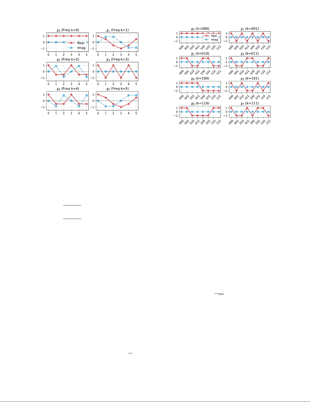
Sp ectral metho ds: crucial for mac hine learning, natural for quan tum computers? V asilis Belis, Joseph Bowles, Rishabh Gupta, Ev an P eters, and Maria Sch uld ∗ Xanadu Quantum T e chnolo gies Inc., T or onto, Ontario, M5G 2C8, Canada (Dated: Marc h 27, 2026) This article presen ts an argument for wh y quantum computers could unlo ck new metho ds for mac hine learning. W e argue that spectral metho ds, in particular those that learn, regularise, or otherwise manipulate the F ourier sp ectrum of a machine learning mo del, are often natural for quan tum computers. F or example, if a generative machine learning mo del is represented by a quan tum state, the Quantum F ourier T ransform allows us to manipulate the F ourier sp ectrum of the state using the entire to olb ox of quantum routines, an operation that is usually prohibitive for classical models. A t the same time, sp ectral metho ds are surprisingly fundamen tal to mac hine learning: A spectral bias has recen tly b een hypothesised to b e the core principle b ehind the success of deep learning; support v ector mac hines hav e been kno wn for decades to regularise in F ourier space, and conv olutional neural nets build ﬁlters in the F ourier space of images. Could, then, quantum computing op en fundamen tally diﬀeren t, muc h more direct and resource-eﬃcient wa ys to design the sp ectral properties of a model? W e discuss this potential in detail here, hoping to stim ulate a direction in quantum machine learning research that puts the question of “why quantum?” ﬁrst. I. INTR ODUCTION In the search for real-world applications for quan tum computers, there is a growing consensus that cryptoanal- ysis and quantum sim ulation are the most mature pro- p osals at this stage, and ﬁnding others “has pro ven re- mark ably diﬃcult” [ 1 ]. Both are also somewhat excep- tional: cryptography is arguably the most structured of all real-w orld problems, and quan tum chemistry shares its v ery theoretical foundations with quantum comput- ers. In this p ersp ectiv e we prop ose a motiv ation for an application area where a clear-cut bridge has b een elusive so far [ 2 ]: machine learning. Besides attracting excessive attention in academic and industrial researc h, quantum machine learning [ 3 – 5 ] has struggled to make a clear case for why quan tum com- puting should b e of fundamental in terest for generalis- ing from data. F or example, sp eeding up linear algebra [ 6 – 9 ] fails to convincingly account for the time it takes to load big matrices into a realistic quantum computer; “Quan tum Neural Net w orks” [ 10 , 11 ] still need to pro ve that they deserve their sp ot in the gallery of scalable, p erforman t models [ 12 – 14 ], and reverting to the analy- sis of “quantum data” [ 15 , 16 ] needs to make a case for wh y lea ving states unmeasured is critical to learn their prop erties in practically relev an t situations. Wh y , then, should we b eliev e that quantum computers are useful for mac hine learning? Here we discuss a p oten tial answer to this question. It rests on the observ ation that “spectral metho ds”—which w e deﬁne lo osely as the design of machine learning mo d- els with desirable prop erties in F ourier space—are funda- men tal to a core principle of learning [ 17 ]: to ﬁnd simple mo dels in expressiv e mo del classes. A t the same time, quan tum algorithms often rely on, or can b e understo o d ∗ In alphabetical order FIG. 1. A common simplicit y bias of mac hine learning models is their smo othness, which is linked to a deca y of the mo del function’s F ourier sp ectrum. But designing such a decay in F ourier space is usually computationally exp ensive. Can quan tum computers help here? b y , F ourier analysis. The main p oint of this pap er is to explain wh y this connection could b e a fruitful starting p oin t for the design of quantum mac hine learning algo- rithms. As an illustrativ e example for the imp ortance of sp ec- tral metho ds in mac hine learning, consider a probability distribution p ( x ) that tells us how lik ely it is to sam- ple a data p oin t x ∈ R N . Simple mo dels intuitiv ely corresp ond to smo oth distributions p ( x ), where we use “smo oth” broadly to mean Lipschitz and inﬁnitely dif- feren tiable functions. Suc h mo dels are robust to input p erturbations: when w e change the input a little, the probabilit y p ( x + δ ) should not change a lot. F urthermore, smo oth models hav e sp ecial prop erties in F ourier space: their sp ectrum deca ys sup er-polynomially (see Figure 1 ). This can b e in tuitively seen by considering the F ourier decomp osition of p ( x ), p ( x ) = 1 √ 2 π Z Ω ˆ p ( ω ) e − 2 π ixω dω , (1) 2 where ˆ p ( ω ) are the F ourier co eﬃcien ts and ω ∈ Ω ⊂ R N the fr e quencies . F unctions that are smo oth will b e com- p osed of weakly oscillating basis functions e − 2 π ixω , and therefore hav e small co eﬃcien ts ˆ p ( ω ) for large frequencies | ω | in Eq. 1 . There has b een gro wing recognition in the machine learning communit y that smo othness is crucial for a mo del to learn and generalise from data. T o this end, an abundance of techniques hav e b een developed for imp os- ing smoothness [ 18 – 21 ]. At the same time, these heuris- tic techniques are indirect and are often computationally ineﬃcien t [ 22 ], and so imp osing mo del smo othness has remained out of reach of these classical metho ds. As sho wn abov e, the important concept of a simplicity bias in learning translates to a clearly deﬁned b ehaviour in F ourier space that can help design mo dels, an idea with a p o w erful group-theoretic generalisation that we will deal with in depth here [ 23 , 24 ]. Giv en that regularisation, or biasing a mac hine learn- ing metho d to wards simple mo dels, is one of the most fundamen tal themes in machine learning, it is curious that sp ectral metho ds enforcing smo othness in F ourier space are not more prominent in the canonical knowl- edge base of researc hers (and, by extension, scarce in the literature of quan tum mac hine learning). A reason migh t b e the computational challenge of working in the F ourier space of a large mo del, whic h is often only accessible indi- rectly via the conv olution theorem. This theorem states that c hanging the F ourier co eﬃcients ˆ f of a mo del by m ultiplying it with a ﬁlter ˆ g in F ourier space corresponds to a con volution in direct space: ( f ∗ g )( x ) = Z X f ( y ) g ( x − y ) dy = F − 1 ( ˆ f · ˆ g ) . (2) In machine learning, the function g —whose F ourier co ef- ﬁcien ts ˆ g mak e up the ﬁlter—is usually kno wn as a (sta- tionary) kernel . As a consequence, a wide range of k ernel metho ds, whic h w ere the workhorse of machine learning in the 1990’s and early 2000’s [ 25 , 26 ] and are widely used for small-to-medium data problems, can b e thought of as sp ectral regularisation metho ds. The same is true for ker- nel to ols like the Maximum Mean Discrepancy employ ed to train implicit generative mo dels [ 27 , 28 ]. Likewise, con volutional lay ers of neural net works, and their group- theoretic generalisations [ 29 , 30 ] such as graph neural net works [ 31 ], design a model class by shaping the F ourier sp ectrum with a ﬁlter (although this ﬁlter acts on the image rather than the mo del function, which is compu- tationally muc h easier). Last but not least, the con v olu- tion theorem helps to empirically prob e ho w deep learn- ing w orks: The sp e ctr al bias hypothesis [ 32 , 33 ] states that the complex mo del class of v astly o v erparametrised neural netw orks learns to match the ground truth’s fre- quency from smallest (i.e., the “smoothest” comp onen t) to largest (the most oscillating comp onen t). All these ob- serv ations p oin t to wards the fact that the F ourier sp ec- trum of a model is a crucial mathematical ob ject to study and design go o d machine learning mo dels, but that we ha ve to rely on indirect access to F ourier space due to computational challenges. Let us no w consider a machine learning mo del that is represen ted b y a trainable [ 34 , 35 ] quan tum state | ψ θ ⟩ . Ho w can quantum computers p ossibly help to access or shap e the mo del’s F ourier spectrum more directly? As w e will see, there are many possible answers to this ques- tion, whic h in timately depend on how the mo del is de- ﬁned, and ho w its spectrum is supp osed to be designed. F or example, if we consider the probabilit y of a mea- suremen t outcome, p ( x ) = |⟨ x | ψ θ ⟩| 2 , as an implicit gen- erativ e mo del [ 36 , 37 ] we can use the Quantum F ourier T r ansform (QFT) [ 38 ] to apply a F ourier transform to the amplitudes of the quan tum state, X x ψ θ ( x ) | x ⟩ → X ω ˆ ψ θ ( ω ) | ω ⟩ . (3) While the QFT is usually associated with the dis- crete F ourier transform of the amplitudes as a func- tion on Z N , this pro cess is kno wn to be eﬃcien t in the n umber of amplitudes for man y groups 1 whic h implies an exp onen tial—or sometimes even super-exp onen tial— sp eedup compared to the classical F ast F ourier T rans- form. Once in the F ourier basis, w e can use the entire arsenal of quan tum algorithms to manipulate the F ourier sp ectrum, for example to imp ose (p ossibly learnable) bi- ases tow ards low er-order coeﬃcients. Another example of ho w quan tum mac hine learning re- lates to spectral metho ds is given by a prominent class of sup ervised quantum machine learning models kno wn as “Quantum Neural Netw orks” [ 10 , 11 ]. These mo dels enco de an input vector x ∈ R N in to a trainable state | ψ θ ( x ) ⟩ , and deﬁne a mo del as an observ able exp ectation f ( x ) = ⟨ ψ θ ( x ) | O | ψ θ ( x ) ⟩ . The standard data-em b edding strategy enco des the entries x i of x via gates of the form exp ( ix i H ), where H is a Hermitian op erator. The resem blance to F ourier basis functions leads to feature maps that hav e elegan t interpretations via F ourier anal- ysis, and induce diﬀerent kinds of sp ectral biases into Quan tum Neural Netw orks [ 39 – 42 ], as well as to dequan- tisation metho ds [ 43 , 44 ]. Here, an emb e dding str ate gy , rather than a QFT, designs the F ourier sp ectrum of a quan tum model. While not a main fo cus of this pap er, we wan t to re- mark that we can also use sp ectral metho ds more in- directly , namely to access more sophisticated algebraic prop erties of the mo del whic h relate to its simplicit y . A p ossible example is a recen t v ariation of the famous quan- tum algorithms solving Hidden Subgroup Problems [ 45 ] suc h as Shor’s algorithm. Giv en several copies of a quan- tum state—whic h ma y represent a generativ e mo del—w e 1 The discrete F ourier transform on the amplitudes is p erformed by the “standard” F ourier transform, while a la yer of Hadamard gates implemen ts the W alsh or “b oolean” F ourier transform, and a rather complicated circuit is known to exist for a F ourier trans- form ov er the symmetric group. 3 can prob e the (un)entanglemen t structure of the state [ 46 , 47 ], whic h op ens up metho ds of inﬂuencing the sim- plicit y of a model in terms of its en tanglemen t. W e b eliev e that these examples are just the tip of a large iceb erg of sp ectral learning metho ds unlo c k ed b y quan tum computers that w ait to b e uncov ered. Our hop e is to stimulate more work in this ﬁeld, and to ﬁnd satis- fying answers to why quan tum theory should fundamen- tally help learning from data—b e it classical or quan tum. Imp ortan t questions are, for example: • Can quan tum mo dels design a soft sp ectral bias without reverting to v ast scales used in deep learn- ing? • Can they extend the success of geometric deep learning to implemen t useful biases, but on in- tractably large mo del spaces (rather than on a tractable image)? • Can group structure help to achiev e tailor-made regularisation for data domains that standard metho ds still struggle with, suc h as graphs, spheres and p ermutations? • What limitations arise from the fact that we can only apply F ourier transforms to amplitudes, but not to probabilities directly? What can we do with the sampling access we hav e to quantum informa- tion? • What are the limitations of classical kernel meth- o ds, and can we go beyond them with sp ectral metho ds in quan tum machine learning? While these questions are wide op en, the goal of this article (which we understand as a mix of p ersp ectiv e, tutorial and review) is to collect the technical to ols nec- essary to start researc h in the spectral approach to quan- tum machine learning. W e will start with a motiv ating example in Section I I that in tends to giv e a concrete intuition for the p oten- tial and pitfalls of sp ectral metho ds in quan tum machine learning. Section I II then lays the mathematical founda- tions of group F ourier transforms. Section IV gives an o verview of sp ectral metho ds in classical machine learn- ing, and, for three examples, shows why the F ourier sp ec- trum of a mo del relates to its simplicity . W e deﬁne the imp ortan t to ol of quan tum F ourier transforms in Sec- tion V and look a little deep er into F ourier sp ectra of states that enco de quan tum models. Finally , Section VI giv es an ov erview of existing lines of research that mak e use of F ourier metho ds in quantum mac hine learning. W e conclude b y commenting on the p oten tial of this ap- proac h. I I. A MOTIV A TING EXAMPLE T o build intuition, we wan t to start with a simple toy example of how a generative quan tum model can be de- signed in F ourier space using the QFT. W e will w ork with binary-v alued data and a simple non-parametric model— a mo del that is directly constructed from the training data with no tunable parameters—to generate samples that are similar to the training examples. The idea is to start with the empirical distribution that only has sup- p ort in the training data, and apply a lo w-pass ﬁlter in F ourier space to “smoothen” this distribution and hence remo ve ﬁnite-sample eﬀects. This principle can b e imple- men ted with quantum and classical metho ds, and allows us to illustrate themes that are encountered rep eatedly when working with sp ectral metho ds in quantum ma- c hine learning: • Desir able mo del pr op erties ar e often explicit in F ourier sp ac e. Here we will use the fact that smo oth models ha ve a deca ying F ourier sp ectrum, whic h w as already discussed in the introduction. • We ne e d to c aptur e the data structur e by using an appr opriate gr oup for the F ourier tr ansform. In this example we use the group Z 2 × Z 2 × · · · = Z n 2 , the set { 0 , 1 } n with addition mo dulo 2. This cap- tures the prop erties of binary random v ariables, and is closely related with quantum computation. • Quantum algorithms c an sometimes act dir e ctly in F ourier sp ac e. Quantum mac hine learning mo dels can often mov e into the F ourier basis, and hence manipulate the F ourier sp ectrum of the amplitudes of a quantum mo del using to ols from the quan tum algorithms to olbox. These tools also deﬁne the fun- damen tal limitations on what we can do. • Quantum metho ds manipulate the F ourier c o eﬃ- cients of amplitudes, not those of the me asur e d in- formation. This prop erty , an implication of the Born rule, can b e a bug or feature of quantum mo del design in F ourier space. Here we will see ho w this prop ert y ampliﬁes the mo del’s desired de- ca y in F ourier space, but mismatches low er-order F ourier co eﬃcients. • The c omputational c ost of quantum and classic al algorithms b ase d on F ourier tr ansforms ar e subtle. W e will sho w that, while in general classically in- tractable, a naive sp ectral design approach can b e classically implemented by a k ernel metho d. A. Smo othness for models ov er binary data Let us start by deﬁning a generative learning problem: Problem 1. L e arning to gener ate bitstrings. Given a tr aining set of bitstrings x ∈ { 0 , 1 } n sample d fr om an unknown distribution p ( x ) , gener ate new bitstrings fr om that distribution. 4 This learning problem is unsolv able without further assumptions, as lots of distributions hav e a high proba- bilit y of generating the training set—ho w can we guess whic h was the right one? As discussed in the introduc- tion, an implicit assumption of man y machine learning mo dels for real-life problems is that the ground truth is smo oth . Informally , smoothness means that data whic h is “close” to high-probability samples also hav e a high probabilit y . Of course, closeness is not alwa ys a clear term when dealing with discrete data. W e will therefore motiv ate the exp e cte d p arities of subsets of bits as a mea- sure of smo othness for binary data, which will turn out to b e F ourier co eﬃcien ts of the mo del p ( x ), at least if we use the appropriate F ourier transform for the group Z n 2 , the Walsh-Hadamar d tr ansform . In tuitively , a probability distribution p : { 0 , 1 } n → [0 , 1], is considered smo oth if its v alue does not change drastically when a small num b er of bits are ﬂipp ed. W e can link this to a prop erty of the p arity functions χ k ( x ) = ( − 1) x · k , (4) where k ∈ { 0 , 1 } n is another bitstring, and x · k is the dot pro duct mo dulo 2, e.g., 101 · 111 = (1 · 1 + 0 · 1 + 1 · 1) mo d 2 = 0. In w ords, the 1-entries of a given k act to select bits in x , and the parity function returns 1 if there are an even num b er of 1s among these bits, and − 1 if there are an o dd num b er of bits. A k is large (and the corresp onding parit y function is of high or der ) if it con tains many 1s, and hence chec ks the parity of a large num b er of bits in x . The n umber of 1s is called the Hamming weight of k . F or a giv en k we can deﬁne the (normalised) exp e cte d p arity of a distribution as E p [ χ k ( x )] = 1 √ 2 n X x ∈{ 0 , 1 } n p ( x )( − 1) x · k . (5) The exp ected parities allow us to mak e the idea of smo othness of probabilistic mo dels ov er binary data pre- cise: Smo oth bitstring distributions hav e exp ected pari- ties that decay for higher orders. This property is easy to in tuitively understand. T ak e, for example, the highest- order k = 1 ... 1: the parity χ 1 .. 1 ( x ) is extremely sensitive to noise in x , as ﬂipping only one bit randomly will al- w ays c hange the parity . A distribution that has a large v alue E p [ χ 1 .. 1 ( x )] needs to hav e v ery diﬀerent probabil- ities for x that are just one bitﬂip aw ay—it is not v ery robust. As mentioned, it turns out that the exp ected parities E p [ χ k ( x )] are the F ourier c o eﬃcients of p ( x ) when us- ing the natural F ourier transform o ver the bo olean cub e (kno wn as the Walsh(-Hadamar d) tr ansform ). As a con- sequence, we can assume from now on that smo oth bit- string distributions ha ve a decaying F ourier spectrum. T o generalise from training data, a go o d strategy is to w ork with a mo del that has a bias tow ards smoothness. This is what we will construct next. B. Smo othing the F ourier spectrum of the data Most generativ e mo dels in mac hine learning, includ- ing most diﬀusion mo dels, energy-based mo dels, ﬂows, and v ariational autoenco ders, deﬁne a mo del class, take a random initial model, and train it to maximize the lik e- liho od of seeing the data. W e could follow this strategy , and construct a class of functions that has a decaying F ourier sp ectrum (in fact, this is what a supp ort vector mac hine do es for sup ervised learning [ 26 ]). But we could also do something more direct (see Figure 2 )—something that could b e elegan tly implemented in a quantum mo del: imp ose a bias directly to the F ourier co eﬃcien ts E p X [ χ k ( x )] = 1 √ 2 n |X | X x ∈X ( − 1) x · k (6) of the empirical distribution p X that only has supp ort on the training data X ⊆ { 0 , 1 } n . These “empirical” F ourier co eﬃcients can b e understo o d as a noisy v er- sion of the true ones. Since the empirical distribution is sparse, its F ourier sp ectrum is dense, and therefore has large higher-order co eﬃcien ts. W e kno w these higher- order coeﬃcients should b e zero for a sm ooth distribu- tion, and so we can therefore consider them to b e ar- tifacts of a ﬁnite data set. In particular, since ( − 1) k · x can b e seen as a Bernoulli random v ariable when x is sampled from p ( x ), the co eﬃcien ts ( 6 ) are un biased esti- mates of the true co eﬃcients ( 5 ) with an absolute error that scales as 1 / p 2 n |X | . Since higher-order co eﬃcien ts are eﬀectively zero for the true distribution, this means that the relative error of the empirical F ourier coeﬃcients is muc h larger at higher order. The sp ectral bias should therefore suppress higher- order co eﬃcien ts, to ensure a smo oth distribution and correct for these ﬁnite-data artifacts. On the other hand, since the low er order co eﬃcients are not zero and w e do not know their v alues a priori, it should not change them m uch b ey ond the 1 / p 2 n |X | estimation error. F or exam- ple, if all training p oints start with a 1 bit, it is reasonable to assume that the exp ected parity of the ground truth for k = 10000 is close to 1, which means that new sam- ples also hav e a 1 bit in this p osition. The idea is hence to “denoise” the data by applying something that would b e called a low-p ass ﬁlter in signal processing. Note that while w e will do this with a “hard” strategy in this didac- tic example, ultimately such a bias will hav e to b e learnt to build p erforman t mo dels (which is why w e suggestiv ely denote the ﬁnal bandlimited model b y a subscript θ ). The c onsiderations so far suggest the follo wing spectral strategy to solv e the generative learning task: Mo del 1. Empiric al smo othing We ar e given a set X of data samples and want to solve Pr oblem 1 . 1. Start with the empiric al distribution p X ( x ) = 1 |X | X x ∈{ 0 , 1 } n I [ x ∈ X ] , (7) 5 FIG. 2. A sketc h of the idea of smo othing an empirical dis- tribution of training samples in F ourier space. The empirical distribution is sparse, with supp ort only on the training data. Therefore, its F ourier sp ectrum is dense and has supp ort on high-order frequencies whic h can b e seen as a consequence of ﬁnite data eﬀects. By applying a low-pass ﬁlter in F ourier space w e imp ose smo othness on the resulting distribution. wher e I is the indic ator function that is one if x is a tr aining sample, and zer o elsewher e. 2. Move into the Z n 2 F ourier sp ac e using the Walsh tr ansform ˆ p X ( k ) = 1 √ 2 n X x ∈X 1 |X | ( − 1) k · x . (8) 3. Apply a (p ossibly le arnable) ﬁlter in F ourier sp ac e that suppr esses higher-or der F ourier c o eﬃcients, but ke eps the lower-or der F ourier c o eﬃcients ap- pr oximately intact. 4. Move b ack to dir e ct sp ac e. 5. Sample fr om the mo del. F or example, w e could apply a decay that depends on the Hamming weigh t of the F ourier co eﬃcient, which is implemen ted in Figure 3 . When we mo ve bac k into direct space, we get a dif- feren t (and typically dense) probability distribution—we ha ve generalised from the training data (see Figure 3 ). In fact, since for b oolean functions the F ourier decom- p osition is a kind of p olynomial decomp osition, what w e just did is a (hard, and not learnable) order-based regu- larisation strategy as suggested in [ 17 ]. C. Implemen tation with quan tum mo dels The strategy sk etched ab ov e can be easily translated in to a quantum algorithm: Mo del 2. Empiric al smo othing with quantum mo dels We ar e again given a set X of data samples and want to solve Pr oblem 1 , but this time we use a quantum state as a gener ative mo del. 1. Start with a sup erp osition of the tr aining data, | ψ X ⟩ = 1 p |X | X x ∈X | x ⟩ (9) 2. Apply the Z n 2 F ourier tr ansform to this state, which is implemente d by applying a Hadamar d gate onto e ach qubit, | ˆ ψ X ⟩ = 1 p 2 n |X | X k X x ∈X ( − 1) x · k | k ⟩ . (10) 3. Apply a (p otential ly non-unitary) quantum tr ans- formation that mo diﬁes the amplitudes of the quan- tum state in F ourier sp ac e. 4. Move b ack into dir e ct sp ac e by applying an inverse F ourier tr ansform, another layer of Hadamar ds. 5. Me asur e in the c omputational b asis to gener ate a sample fr om the mo del. It is imp ortan t to note that manipulating the F ourier sp ectrum of the amplitudes ψ ( x ) (Step 3) of the quan tum state is an indirect wa y to manipulate those of the me a- sur ement distribution (i.e., the ﬁnal prob abilistic mo del), whic h is given b y the Born rule, p ( x ) = | ψ ( x ) | 2 . (11) The F ourier co eﬃcien ts of ψ ( x ) and p ( x ) are related by an auto con v olution, as we will see in Section V C . Compar- ing Figures 3 and 4 sho ws that the spectral manipulation of amplitudes leads to an attenuated proﬁle of the ﬁnal mo del compared to the same manipulation b eing applied to probabilities. F urthermore, unitary transforms on the amplitudes can lead to non-line ar transformations of the distribution’s F ourier sp ectrum. Depending on the appli- cation, working with amplitudes can therefore b e a bug or feature for mo del design. Of course, quan tum computing imp oses fundamental constrain ts on how to manipulate the F ourier spectrum of the state in Step 3. F or example, we can naively im- plemen t the noise ﬁlter used in Figure 3 on the ampli- tudes as shown in Figure 4 by using a quantum algo- rithm that conditionally rotates an ancilla state by an angle of 2 arcsin(1 − 2 θ ) when a 1 is encountered in | k ⟩ . P ost-selecting on the ancilla, we end up with a state that re-w eighted the amplitudes in F ourier space according to the noise ﬁlter. A fundamen tal limitation of this sim- ple approac h is the success probabilit y of post-selection, whic h prohibits arbitrarily strong bandlimiting at large scales. More sophisticated techniques [ 48 , 49 ] may b e able to push the b oundaries, but alwa ys incur a price for highly non-unitary operations. A more successful approac h may inv olv e opting for a unitary la yer that—rather than attempting to bandlimit the amplitudes of the quantum state probabilistically— applies a deterministic phase mask to the amplitudes so 6 FIG. 3. An example of smo othing an empirical distribution in F ourier space to solve the generative learning problem. Starting from an empirical distribution p X of four binary data samples (top left), we compute the (W alsh) F ourier sp ectrum (bottom left). W e then apply a ﬁlter of the form ˆ p θ ( k ) = (1 − 2 θ ) | k | ˆ p X ( k ), where θ ∈ [0 , 1] controls the sp ectral decay rate. Mo ving bac k into direct space, we get a mo del that generalised from the training data by making the empirical distribution smo other. that the resulting in terference from autoconv olution au- to correlation results in an eﬀective low-pass ﬁlter on the sp ectrum of the mo del’s probability distribution. Ultimately , a ﬂexible model also requires the transfor- mation to b e learnt, whic h suggests the use of scalable v ariational circuits that come with an additional set of c hallenges. 2 In summary , quan tum computers can eﬃ- cien tly manipulate the F ourier sp ectrum of the ampli- tudes of a quantum mo del state, but if we can design go od F ourier ﬁlters within the constraints of quantum algorithms will be a crucial question for sp ectral meth- o ds in quan tum machine learning. D. Wh y empirical smo othing ma y b e classically hard W e saw that our to y example for a spectral metho d, generativ e empirical smo othing, can at least in princi- ple b e implemented eﬃcien tly on a quantum computer. But ho w computationally feasible is this strategy classi- cally? In these last tw o sections we will argue that brute force approaches are doom ed to fail, but that care has to b e tak en when claiming speedups, as some situations allo w for implicit wa ys to eﬃciently implement empirical smo othing. First, let us hav e a lo ok at eﬃciently computing prob- abilities p ( x ) after classical empirical smo othing. This abilit y would unlo c k training a classical mo del, for ex- ample by taking the mo del class of bandlimited empiri- cal distributions and learning the bandlimiting ﬁlter us- 2 In up coming w ork w e study a learnable diagonal phase mask implemented by trainable IQP circuits [ 14 ] as a suitable ansatz to build ﬁlters. ing maxim um likelihoo d estimation. Computing the k ’th F ourier co eﬃcient of the empirical distribution, ˆ p X ( k ) = 1 √ 2 n X x ∈X ( − 1) k · x , (12) is eﬃcient, as it is a sum o v er tractably many terms. Of course, there are exponentially many such F ourier co eﬃ- cien ts. Computing a single probability from an empirical distribution that has b een bandlimited to contain only a small num b er of terms, p θ ( x ) = 1 √ 2 n X k ∈ Ω ˆ g ( k ) ˆ p X ( k )( − 1) k · x , (13) is tractable. Lik ewise, computing marginal distributions b ecomes tractable (by sampling ov er subsets of F ourier co eﬃcien ts), whic h allows us to compute conditional probabilities, opening up the abilit y to sample from p θ ( x ) in an autoregressive manner. Is empirical smo othing then classically tractable? The issue is the numb er of F ourier co eﬃcients to keep trac k of. F or high dimensions, bandlimiting would hav e to b e limited to a few frequencies in each dimension. F or example, in the slo west-gro wing case of Z n 2 , where there are tw o frequencies in eac h dimension, the num ber of F ourier frequencies with Hamming weigh t | k | less than some threshold b is given b y P b m =0  n m  . F or n = 10 , 000 dimensions and b = 2, we would already hav e to sum o ver 50 million F ourier co eﬃcients to compute the prob- abilit y of a data p oint, even for the simplest bandlim- ited model. F or other groups and larger thresholds, this quic kly b ecomes unfeasible. F urthermore, to keep em- pirical smo othing classically tractable, the ﬁlter for the k ’th co eﬃcient cannot dep end on the F ourier co eﬃcien ts other than ˆ p ( k ), as there are intractably many of these (ev en for the empirical distribution). These tw o problems 7 FIG. 4. An example of smoothing empirical distributions with quantum computers, using the same ﬁlter as in Figure 3 . F ourier ﬁltering is performed on the amplitudes of the quantum state. W e encode the empirical distribution (top left) in to a sup erposition | ψ X ⟩ (mid left), to whic h w e apply the (W alsh) F ourier transform (b ottom left). W e then apply a non-unitary transformation (with the help of ancillas) to implement the ﬁlter ˆ ψ θ ( k ) ∝ (1 − 2 θ ) | k | ˆ ψ X ( k ) (b ottom right). Moving back in to direct space (mid right), we get a quantum mo del with a new distribution of amplitudes, whose measurement distribution constitutes the generativ e mo del. Comparing to Figure 3 , it is clear that manipulating the F ourier coeﬃcients of the amplitudes of a quan tum model leads to a diﬀeren t generative mo del, but with a similar structure: high probabilities are ampliﬁed and lo w ones suppressed. clearly do not o ccur for the quan tum computer, which means that empirical smoothing migh t displa y quantum sp eedups for the useful task of generalisation. Of course, whether this strategy is able to solv e problems that other approac hes to generalisation cannot is an op en question. As a cautionary tale, we wan t to conclude our analysis of this toy example by showing that for a sp eciﬁc ﬁlter it c an be p ossible to eﬃciently sample from a bandlimited empirical distribution on a classical computer. The tric k is to use conv olution with a k ernel, a metho d that we will discuss later as the standard classical approach for sp ectral mo deling, and hence the most viable “classical comp etitor” for this approach to QML. E. Example of a dequan tisable ﬁlter While we argued that the direct manipulation of the F ourier sp ectrum required in I I B is not computationally feasible in general, it might very w ell b e p ossible for very sp eciﬁc F ourier ﬁlters. T o illustrate this, consider the noise ﬁlter used as an example in Figure 3 : ˆ p θ ( k ) = (1 − 2 θ ) | k | ˆ p X ( k ) , (14) where the hyperparameter θ ∈ [0 , 1] con trols the deca y rate. Going bac k in to direct space, we get the mo del p ( x ) = X x ∈{ 0 , 1 } n p X ( x ) κ ( x − y ) , (15) with κ ( x, y ) = θ d H ( x,y ) (1 − θ ) n − d H ( x,y ) , which is known as the noise kernel . The mo del can therefore b e imple- men ted b y a conv olution p X ∗ κ in direct space. A t the same time, p ( x ) is a t ypical kernel density estimation mo del, a class of models which deﬁne probabilit y distri- butions as sums of kernel functions cen tered around the training data. Crucially (and this is only true in rare cases), the k ernel has the prop ert y that we can sample from p ( x ) even in high dimensions: we simply sample a training data p oin t and ﬂip each bit with probability θ . This example shows that for some manipulations in F ourier space, kernel metho ds can ev en b e used for gen- erativ e models. Clearly , there are a lot of restrictions on the kernel to mak e this work, but k ernel methods ha ve already b een used to dequantise a range of sup ervised quan tum machine learning models [ 43 , 44 ] and are a con- tender for spectral metho ds. In summary , the simple example of empirical smooth- ing show ed how (group) sp ectral metho ds in mac hine learning can b e interesting for machine learning and nat- ural for quantum computers. But it also highlighted 8 subtleties that ha ve to b e handled when designing quan- tum mac hine learning mo dels—suc h as the Born rule, the diﬃcult y of manipulating amplitudes, and p ossible clas- sical dequantisation with kernel metho ds. These c hal- lenges appear in man y (but not all) sp ectral approac hes to quantum mac hine learning. With this illustrative case in mind, let us now get back to the main argumen t: why quan tum computers migh t be useful to implemen t sp ec- tral metho ds in machine learning. I II. SPECTRAL METHODS As mentioned, w e lo osely consider sp e ctr al metho ds for machine le arning as those that design machine learning mo dels by manipulating their prop erties in F ourier space. In this section we will rigorously deﬁne what w e mean by terms like “F ourier sp ectrum” and “F ourier co eﬃcients”, in particular in their group-theoretic generalisation. A. Motiv ation What do F ourier transforms hav e to do with groups? Ev erything, if one lo oks closely . Let us motiv ate this with one of the most well-kno wn F ourier transforms, the discr ete F ourier tr ansform . It transforms a sequence f 1 , ..., f d of complex n umbers in to another sequence of complex num b ers. Sometimes the complex v alues are written as a function f ( x ) ev aluated or “sampled” at regular in terv als, for example using integer v alues x ∈ { 0 , ..., d − 1 } . The F ourier coeﬃcients are then given as ˆ f ( k ) = 1 √ d d − 1 X x =0 f ( x ) e 2 π i kx d , (16) where the frequencies k are also in { 0 , ..., d − 1 } . The in verse F ourier transform is given as f ( x ) = 1 √ d d − 1 X k =1 ˆ f ( k ) e − 2 π i kx d , (17) Note that the normalisation factor is a matter of con- v ention, and we will here alwa ys use the “balanced” v ersion which uses the same pre-factor for the F ourier transform and its in verse, and k eeps the L 2 normalisa- tion of the F ourier coeﬃcient constan t. The expressions e 2 π i kx d corresp ond to F ourier basis functions with in teger- v alued frequencies k , and a F ourier co eﬃcient ˆ f ( k ) can b e seen as the pro jection of f ( x ) on to the k ’th basis function. The function b ey ond the interv al 0 , .., N − 1 is thought to b e “p erio dically contin ued”, which means that f ( x ) = f ( x + N ). But why do—at least if we do not w ant to incur ad- ditional headaches—the x v alues hav e to b e equidistant? Wh y this notion of “p eriodic contin uation”? Wh y are the basis functions of exp onential form? Wh y are the k also in tegers? And what makes the F ourier basis special? It turns out that all of these questions ha v e an elegant answ er if w e in terpret the function domain as a group. As a reminder, a group is a set of elements that has: 1. an op eration that maps tw o elements a and b of the set in to a third elemen t of the set, for example c = a + b , 2. an “identit y element” e such that e + a = a for any elemen t a 3. an inv erse − a for every element a , such that a + ( − a ) = e . An A b elian gr oup has the property that g g ′ = g ′ g . Its char acters are functions χ : G → C with the prop ert y χ ( g g ′ ) = χ ( g ) χ ( g ′ ). Returning to the discrete F ourier transform, w e can consider the x as elemen ts from the set of integers { 0 , ..., d − 1 } , together with a prescription of how to com- bine tw o integers to a third from this set. Cho osing “ad- dition mo dulo N” for this op eration (which means that ( d − 1) + 1 = 0), w e get the cyclic gr oup Z d . This c hoice explains the equidistant property: in tegers are by nature equally spaced in R . It also explains the perio dic contin u- ation, as x = x + d implies f ( x ) = f ( x + d ). F urthermore, the in teger-v alued frequencies k turn out to b e elemen ts from the so-called “dual group” ˆ G , which in this case lo oks exactly lik e the original one. Finally , the F ourier basis functions are exactly the characters of Z d (whic h form a basis of the space of functions on G ), and the F ourier co eﬃcients hence the pr oje ction of f ( x ) onto the char acters . Note that other standard F ourier transforms can b e asso ciated with groups as well: A F ourier series trans- forms p erio dic functions on the real line with perio d 2 π , whic h corresp onds to the domain R / Z , while a c ontin- uous F ourier tr ansform on real n umbers relates to the group ( R , +) (the real num b ers under addition). Mul- tiv ariate functions, like those ov er R N , are then deﬁned o ver direct pro ducts of groups. B. Group F ourier transforms F or simplicit y , we will focus on discrete groups—which are most relev an t for qubit-based quan tum computing— and follo w the insightful presen tation in [ 24 ]. Con tin uous F ourier transforms ov er lo cally compact groups simply turn the sum into an integral ov er a Haar measure on G . F or discrete Abelian groups, the standard F ourier transforms generalise as follows: Deﬁnition 1. F ourier tr ansform over Ab elian gr oups L et G b e a discr ete A b elian gr oup and χ k its char- acters fr om the Pontryagin Dual gr oup ˆ G . The F ourier tr ansform F maps a function f : G → C to a function 9 ˆ f : ˆ G → C : ˆ f ( k ) = 1 p | G | X g ∈ G f ( g ) χ ∗ k ( g ) . (18) The inverse F ourier tr ansform, implementing the r everse map, c omputes the function f ( g ) = 1 p | G | X k ∈ ˆ G χ k ( g ) ˆ f ( k ) . (19) Again, the normalisation of forward and reverse F ourier transform, and whic h one carries the conju- gate of the character, is a conv ention, and sometimes χ k ( g − 1 ) = χ ∗ k ( g ) is used. The F ourier transform ov er a discrete, lo cally com- pact non -Ab elian group lo oks slightly diﬀerent from the Ab elian F ourier transform. Instead of the c haracters of the group, they inv ok e ob jects called the irr e ducible r epr esentations or irr eps . A r epr esentation is a map R : G → GL ( V ) from group elemen ts to linear trans- forms on a vector space V . There are many represen ta- tions for a given group, each referring to a diﬀerent vector space. A subspace W ⊆ V is called invariant if for every group element g ∈ G and ev ery vector w ∈ W , the result R ( g ) w is still inside W . The representation is said to b e irr e ducible if the only inv ariant subspaces are the trivial zero space { 0 } and the entire space V itself. With this, we can deﬁne the most general version of the group F ourier transform as follows: Deﬁnition 2. F ourier tr ansform over non-A b elian gr oups L et G b e a discr ete non-Ab elian gr oup and R the set of its (matrix-value d) ine quivalent irr e ducible r ep- r esentations. The F ourier tr ansform maps a function f : G → C to the matrix-value d F ourier c o eﬃcients ˆ f ( σ ) = 1 p | G | X g ∈ G f ( g ) σ ( g ) † , (20) with σ ∈ R . The inverse F ourier tr ansform is given by f ( g ) = 1 p | G | X σ ∈R d σ tr { ˆ f ( σ ) σ ( g ) } , (21) with d σ the dimension of the irr ep σ . In the non-Ab elian case, the F ourier co eﬃcien ts are matrices of v arying sizes (and hence basis dep enden t, whic h can complicate their interpretation). Note that the Ab elian case is a sp ecial case of Deﬁnition 2 , as the ir- reps of an Ab elian group are one-dimensional, and hence equal to their traces, i.e., the c haracters. C. Con volution Giv en the prominent role of the conv olution theorem [ f ⋆ g ( σ ) = ˆ f ( σ ) ˆ g ( σ ) , (22) it is useful to also deﬁne the group-theoretic generalisa- tion of con volution: ( f ⋆ g )( g ) = X g ′ ∈ G f ( g ( g ′ ) − 1 ) g ( g ′ ) . (23) F or Ab elian groups, where the group operation is usually denoted by a +, while adding an in v erse elemen t becomes a − , this b ecomes the more familiar ( f ∗ g )( x ) = X y ∈ R f ( x − y ) g ( y ) . (24) Note that in machine learning, con volution is often con- ﬂated with the more common cr oss-c orr elation , which replaces the min us sign with a plus. D. Symmetry of the F ourier basis The inv erse F ourier transform can b e understoo d as a decomposition of a function o v er G . Ac- cording to the Peter-W eyl theorem, the irrep en tries { σ ij } σ ∈R ,ij ∈{ 1 ,...,d σ } form a complete orthogonal basis of L 2 ( G ), the space of square integrable functions on the group. But what is so sp ecial about the F ourier basis? A deﬁning feature of the F ourier basis is that the sub- spaces L σ ⊆ L 2 ( G ) spanned by the set of all irrep entries { σ ij ( g ) } for a giv en σ are invariant under the gr oup ac- tion . This follows from the deﬁnition of a represen tation: σ ( g g ′ ) = σ ( g ) σ ( g ′ ) , (25) whic h means that a translation b y g ′ do es not cause the function to lea ve the inv ariant subspace L σ = span { σ 11 ( g ) , σ 12 ( g ) , . . . , σ d σ ,d σ ( g ) } . (26) F or Ab elian groups (using additive notation b elow), where we index the dual group by k ∈ ˆ G , the irreps are one-dimensional. This means the in v arian t subspaces L k = span { χ k (g) } are each spanned by a single c haracter that fulﬁlls χ k ( g + g ′ ) = χ k ( g ) χ k ( g ′ ) , (27) The signiﬁcance of this in v ariance property is discussed at length in the w ork of Diaconis [ 23 ]. F or example, if the symmetric group acts by p erm uting the features of a data vector, this in v ariance means that the F ourier pow er sp ectrum (the energy captured within each in v arian t sub- space) do es not c hange if we permute the order of the features, which is often an arbitrary lab eling decision. This is in timately related to the smo othness inheren t in the F ourier sp ectrum: it informs us how the function transforms if we shift it in direct space. In this sense, the F ourier basis can capture imp ortan t structure in the data under “shifts”, whic h helps quan tify its simplicit y for the design of machine learning models—a claim that w e will supp ort with more evidence in the next section. 10 FIG. 5. Illustration of the relation betw een a group and a homogeneous space, which are spaces where every p oint can b e reached by acting with a group elemen t. Group elemen ts that map to the same p oin t live in cosets of the stabiliser subgroup (whose elements map x 0 to itself ). W e can asso ciate the homogeneous space with the quotient space G/H . E. F ourier transforms on homogeneous spaces While we fo cus on sp ectral methods for functions on groups in this pap er, there is an important generalisation to functions on the homo gene ous sp ac e X that a group G acts on . (W e will denote a group action as ▷ : G × X → X with g ▷ x = x ′ .) This opens up the realm of sp ectral analysis to man y more data t ypes, which is why w e will brieﬂy list the relev an t deﬁnitions here. T ec hnically , a homogeneous space X is a space where the group G acts transitiv ely (see Figure 5 ). This means one can get from any p oin t x ∈ X to any other p oint y ∈ X using a group operation, g ▷ x = y . Let us denote as H the stabilizer sub gr oup of an arbitrary reference point x 0 ∈ X , H = { h ∈ G | h · x 0 = x 0 } . (28) The cosets g H = { g h | h ∈ H } of the stabiliser subgroup are sets of group elemen ts whose action maps x 0 on to the same p oin t x ∈ X . This means that eac h p oin t in X can b e associated with a coset of H in G . This allows us to asso ciate X with the quotien t space, X ∼ = G/H . T o sp ectrally analyze a function f : X → C , we can therefore interpret it as a function f : G/H → C and then “lift” it to G by making it constan t on all group elemen ts in the same coset (i.e, the blue regions in Figure 5 ). W e deﬁne the lifte d function f ↑ : G → C b y f ↑ ( g ) = f ( g ▷ x 0 ) . (29) Mathematically , this symmetry means that f ↑ is righ t- in v arian t under H : f ↑ ( g h ) = f ( g h ▷ x 0 ) = f ( g ▷ x 0 ) = f ↑ ( g ) ∀ h ∈ H . (30) W e can no w apply the standard F ourier T ransform to f ↑ : ˆ f ↑ ( ρ ) = X g ∈ G f ↑ ( g ) ρ ( g ) † . (31) The technique of lifting has enabled the use of group F ourier transforms to rigorously iden tify conv olutional la yers with group-equiv ariant transformations, which ga ve rise to generalisations of conv olutional neural net- w orks [ 30 ] in machine learning research. It is also re- lated to one of the ﬁrst formulations of hidden subgroup problems, which Kitaev phrased as an Ab elian stabiliser problem in 1995 [ 50 ]. In the following w e will con tinue to fo cus on F ourier transforms of functions on groups rather than homogeneous spaces, but ackno wledge the potential that lies in this simple extension of sp ectral analysis. IV. CR UCIAL FOR MACHINE LEARNING Smo othness is desirable in machine learning because it leads to robust models that generalise well [ 22 ], and has motiv ated many metho ds [ 18 – 21 ] that aim to bias models to wards smo othness. Y et, these tec hniques are scattered and act indirectly on the mo del sp ectra, suggesting the need for a broader paradigm for directly imposing sim- plicit y biases. Thus, b efore discussing quantum mac hine learning algorithms, w e ha ve to address the elephant in the ro om: Why should F ourier space b e a prime place to design the learning prop erties of a mac hine learning mo del? The argument of this pap er, which we presen t in more detail here, is that machine learning fundamen- tally needs to imp ose biases tow ards “simple mo dels”, and that the F ourier sp ectrum captures what is meant b y “simple”—for “conv entional” data types as well as for more sp eciﬁc, group-structured data such as p erm u- tations. T o that end, w e will ﬁrst review the role of simplicity and regularisation in learning theory . W e will then tak e a closer lo ok at the notion of simplicit y captured by the lo w-order part of the F ourier sp ectrum for three example groups, which show cases the div ersity in which “simple” can be in terpreted. Lastly , w e will highligh t that spectral metho ds are already quite prominent in mac hine learning ev en if they are hardly ev er explicitly men tioned in text- b ooks: they are implicitly used in metho ds that in volv e (stationary) k ernels, such as con volutional neural nets, supp ort vector mac hines, the maximum mean discrep- ancy to train Generativ e Adv ersarial Net works (GANs), and the Neural T angent Kernel that b ecame a prime framew ork to inv estigate the working principle of of deep learning. A. Wh y a simplicit y bias is crucial for mac hine learning The foundations of learning theory [ 51 , 52 ] cast ma- c hine learning as the problem of balancing expressivity and simplicity in mo dels built from data. This is made particularly concrete in the framework of statistic al le arn- ing the ory dev elop ed by V apnik and Chervonenkis [ 53 ], whic h quantiﬁes the generalisation p o wer of a sup ervised 11 mo del through the principle of empiric al risk minimiza- tion . In this framework, the goal of machine learning is to learn some function f from a set of p ossible functions H that minimizes the exp e cte d risk R ( f ) = Z X p ( x, y ) L ( f ( x ) , y ) dxdy , (32) whic h represents the mo del’s p erformance on unseen data dra wn from a ground truth distribution p ( x, y ) with re- sp ect to some loss metric L . Practically , R ( f ) is exactly what the test err or is supp osed to measure. Since p is unkno wn, machine learning practitioners try to minimise the exp ected risk by minimizing the empiric al risk ˆ R M ( f ) = 1 M X x ∈ data L ( f ( x ) , y ) , (33) the av erage error on a training set of size M . Imp or- tan tly for us, learning theory typically upp er b ounds the exp ected risk by the empirical risk, plus a term C ( H ) that accounts for the c ap acity of the mo del [ 54 , 55 ], R ( f ) ≤ ˆ R M ( f ) + C ( H ) . (34) T o get a small exp ected risk (or test error), one has to decrease b oth terms on the right hand side. How ever, these terms are at odds with eac h other. This is some- times captured in the “bias-v ariance-tradeoﬀ ”, a term that refers to the high v ariance of mo dels that ha ve a lo w training error (as they ov erﬁt the particular data, and pro duce v ery diﬀerent predictions when trained on diﬀeren t training data sets), and a high bias of those that are simple (as they cannot learn the in tricacies of the pat- tern). Learning, as a conclusion, is the art of balancing the mo del capacit y with its ﬂexibility . The adven t of deep learning has brought some more n uance into this picture. In the past, the capacit y term w as c hosen to capture the expressivity of the mo del’s function class, such as the VC-dimension [ 53 ] that mea- sures ho w ﬂexible the decision b oundary of the b est func- tion in the mo del class is, or the R ademacher c omplex- ity [ 56 ] that measures the av erage capacit y of a mo del class to classify randomly assigned lab els. When deep learning sho wed increasing evidence of empirical suc- cess, one of the biggest “mysteries” was wh y large neu- ral net works—a mo del class that has an arbitrarily large term C ( f ) under these measures, as it can learn even unstructured lab els [ 57 ] — ge neralises so well. The res- olution was found in the in terplay of large models, big data and the optimisation algorithm (i.e., [ 58 – 61 ]): some- ho w, when these come together, the mo dels that are ef- fectiv ely found in training are simple, even though train- ing c ould in principle ﬁnd m uch more complex mo dels that do not generalise. In other w ords, deep learning has a hidden, or “implicit” regularisation bias. This bias seems to—somewhat paradoxically—fundamen tally rely on scale: the lottery ticket hyp othesis [ 62 ] suggests that while tr aine d neural netw orks are rather compressible (i.e., “simple”), they cannot b e found using smaller arc hi- tectures that are tailor-made to the solution. Altogether, the insights from deep learning were well summarised by Wilson’s soft simplicity bias : “rather than restricting the h ypothesis space to a void ov erﬁtting, [go od mo dels] embrace a ﬂexible hypothesis space, with a soft prefer- ence for simpler solutions that are consisten t with the data”. [ 17 ] B. Ho w a F ourier sp ectrum deﬁnes simplicit y If w e understand machine learning as the problem to ﬁnd expressive, scalable mo del classes that ha ve a sim- plicit y bias, a ma jor component of designing go od mo d- els is to engineer the simplicity bias. F or deep learning, this happ ened somewhat accidentally , and relies on hea vy computational resources. An imp ortan t op en question is hence how to engineer “soft simplicity biases” more consciously , and hopefully without the immense energy requiremen ts of large neural netw orks. W e will now explore in more depth why the F ourier sp ectrum provides a useful mathematical framework to deﬁne—and subsequently exploit—notions of smo oth- ness. This connection is relatively straightforw ard for the standard F ourier transform on ( R , +), where the co- eﬃcien ts capture smo othness, and on Z N 2 , where they capture correlations and interaction eﬀects. Building on this, w e will present an in tuition for the F ourier sp ectrum of the non-Abelian symmetric group S n , whic h captures signiﬁcan tly more complex correlation patterns. Before pro ceeding, w e emphasize that our notion of smo othness in b oth the Ab elian and non-Ab elian cases dep ends on some assumptions. While we ma y alwa ys de- ﬁne smo othness from ﬁrst principles in terms of a partic- ular set of generators, w e generally rely on empirical data and prior b eliefs in order to c ho ose a natural set of gen- erators that b est describ es our observ ations in terms of smo oth functions. In this wa y , the treatmen t considered here may b e generalised to a large class of group-theoretic settings. 1. Continuous fe atur es The standard c ontinuous F ourier tr ansform , whic h we men tioned in the introduction, transforms functions on the group R (or more precisely , ( R , +)), with characters exp (2 π ixk ). Its m ultidimensional version maps functions on pro ducts of this group, R N . The F ourier co eﬃcien ts of a function ov er R N are related to its smo othness . The most obvious connection b et ween the F ourier sp ec- trum and smo othness of a b ounded function on R N is giv en by the canonical deﬁnition of smo oth functions as inﬁnitely diﬀeren tiable. One can show that such functions ha ve a sup er-p olynomial asymptotic decay in 12 FIG. 6. F ourier basis functions χ k ( x ) for the cyclic group Z d with imaginary part in blue and real part in red. F ourier space, or | ˆ f ( ω ) | = O  | ω | − m  as | ω | → ∞ . (35) Using the formula for partial integration, and assuming that f decays at ±∞ , one can write a F ourier coeﬃcient ˆ f ( k ) as the F ourier coeﬃcient of the deriv ativ e of f , ˆ f ( k ) = Z dxf ( x ) e − 2 π ikx (36) = 1 (2 π ik ) m Z dx ( ∂ m x f ( x )) e − 2 π ikx (37) = 1 (2 π ik ) m \ ∂ m x f ( x ) . (38) Bounding | \ ∂ m x f ( x ) | by the ﬁnite L 1 norm of the input function here one sees that | ˆ f ( k ) | ≤ c/k m (39) for some constant c , which is a spectral decay with the p o w er of m . If m go es to inﬁnity , the asymptotic decay has to b e faster than an y p olynomial, and hence “sup er- p olynomial”. This conﬁrms the in tuition w e ha v e from signal pro cessing, namely that smo oth functions hav e to b e constructed from slowly oscillating basis functions: their F ourier coeﬃcients are concen trated in the lo wer- order part of the spectrum. W e wan t to brieﬂy note that some encoding strate- gies in quantum mac hine learning represen t data as com- putational basis states. In these cases we cannot w ork with R N , but we can limit the data to a contin uous in terv al in each dimension, which w e chop into d bins. This allows us to w ork with a ﬁnite-precision approxima- tion of R N expressed by pro ducts of the cyclic group, Z N d = Z d × · · · × Z d . Figure 6 shows that the real and imaginary part of its characters exp (2 π i xk d ) are in- deed “coarse-grained” sine and cosine functions. A sim- ilar pro of to ab o ve can b e used to link the “mo dulus of FIG. 7. F ourier basis functions χ k ( x ) for the b o olean group Z n 2 with imaginary part in blue and real part in red. smo othness” of a function ov er this Ab elian group to a deca y in F ourier space. 2. Binary fe atur es In Section I I w e saw the Walsh tr ansform that acts on functions on a pro duct of cyclic groups with t w o ele- men ts, Z 2 × · · · × Z 2 = Z n 2 . This group can b e thought of as the set of bitstrings x ∈ { 0 , 1 } n with addition mo dulo 2, and giv es rise to bo olean cube arithmetic. W e also sa w that the F ourier co eﬃcien ts of a probability distribution o ver the group Z n 2 can be interpreted as exp ected parities of subsets of bits: The 1s in the frequency k ∈ { 0 , 1 } n de- ﬁne which bits are selected, and the Hamming w eight of k deﬁnes the or der of the frequency . The parity functions in Eq. 4 are nothing but the characters e iπ x · k = ( − 1) x · k (where x · k is the bitwise inner product mo dulo 2), and the k are elements from the dual group. The F ourier co eﬃcien ts are then written as ˆ f ( k ) = 1 √ 2 n f ( x ) e iπ x · k . (40) W e will no w sho w why the F ourier co eﬃcients of a probabilit y distribution ov er Z n 2 also hav e other statis- tical interpretations, namely as moments when f is a probabilit y distribution, and inter action eﬀe cts if it is a resp onse function (as kno wn in the literature on experi- men tal designs [ 63 ]). T ogether these insights show that the low er-order characters of Z n 2 , and hence low-order frequencies of a model, ha ve rich interpretations as the statistically simple part of a mo del. Moments . Remember that a moment of a probabilit y 13 distribution p ( x ) is deﬁned as 3 E [ x k ] = X x p ( x ) x k . (41) F or multiple binary random v ariables x 1 , ..., x n , a mixed momen t of order k = k 1 + · · · + k n is given as E [ x k 1 1 . . . x k n n ] = X x 1 ,...,x n p ( x 1 , ..., x n ) x k 1 1 . . . x k n n . (42) F or binary random v ariables, the k 1 , ..., k n ha ve to be in { 0 , 1 } as x 2 i = x 0 i , x 3 i = x 1 i , etc. The relation betw een mo- men ts and F ourier co eﬃcien ts is exp osed if, for the mo- men t, w e mov e to a group that is p erfectly isomorphic to Z 2 , namely the second-order cyclic group ( {− 1 , 1 } , × ) of a “spin v ariable” under m ultiplication. With this c hange, i.e., if we deﬁne our mo del distribution on ¯ x ∈ {− 1 , 1 } n instead of x ∈ { 0 , 1 } n , the F ourier c o eﬃcients of p ( ¯ x ) ar e pr e cisely its moments . This can b e seen since ( − 1) kx = Y i | k i =1 (1 − 2 x i ) = Y i | k i =1 ¯ x i (43) where x i , k i is the i ’th bit of x, k . As the shape of the function do es not change when mo ving from one group to its isomorphic equiv alen t, w e can in tuitively in terpret F ourier co eﬃcien ts of Z n 2 as moments. Consequen tly , constructing mo dels with a decaying F ourier sp ectrum deﬁnes a mo del class that captures only low-order mo- men ts. It is imp ortan t to note that this link is a sp ecial prop ert y of Z n 2 . More generally , the F ourier sp ectrum can b e deﬁned as the char acteristic function of a proba- bilit y distribution, and the momen ts can b e “generated” b y taking partial deriv atives of that function. How ev er, w e will see b elow that also for the symmetric group, lo w- order F ourier co eﬃcien ts capture some kind of low-order correlation. Inter action eﬀe cts. It turns out that a ﬁeld of statistics called “exp erimen tal design” [ 63 ] oﬀers an alternative, v ery in tuitive in terpretation for the F ourier co eﬃcients of a b oolean function f ( x ), x ∈ { 0 , 1 } n as so-called inter- action eﬀe cts , which capture ho w muc h a c hange in one v ariable aﬀects the inﬂuence that other v ariables ha v e on f . W e will illustrate this with a small example. Imagine that bistrings x signify combinations of drugs, mo deled by features x 1 , ..., x n that can either be admin- istered ( x i = 1) or not ( x i = 0) for i = 1 , ..., N . F or no w, consider every possible combination x ∈ { 0 , 1 } n of N drugs was tested in a large trial, and the resp onse f ( x ), such as a reco very rate of patients, was measured. 4 3 F or ease of notation, we will not use diﬀerent symbols for a ran- dom v ariable X and its realisation x as standard in the statistics literature. 4 In so-called fr actional factorial designs statisticians look at trials that did not include all x treatment com binations, which is muc h closer in spirit to our ultimate goal to work with ﬁnite data. A crucially imp ortant question is how the ﬁrst drug x 1 inﬂuences f ( x ), but indep endent of whether or not we administered drug x 2 . W e can do this by measuring the diﬀerence b et ween the resp onse for x 1 = 1 and x 1 = 0, a veraged ov er all possible v alues of a ﬁxed x 2 : L ( x 1 ) =  f (10) − f (00)  +  f (11) − f (01)  . (44) The same is true for the inﬂuence of x 2 on f : L ( x 2 ) =  f (01) − f (00)  +  f (11) − f (10)  . (45) The ab o ve can be summarised b y introducing the c ondi- tional eﬀe ct L ( x 1 | x 2 = a ) =  f (1 a ) − f (0 a )  , (46) and writing L ( x 1 ) = L ( x 1 | x 2 = 0) + L ( x 1 | x 2 = 1) . (47) Finally , we can ask ho w the drugs interact, for instance ho w the change in resp onse function f when c hanging x 1 diﬀers when w e c hange x 2 . (This is in fact a sec- ond deriv ative, it is the change of the change.) The in- teraction can b e deﬁned b y taking the diﬀerence of the conditional eﬀects abov e: L ( x 1 x 2 ) = L ( x 1 | x 2 = 1) − L ( x 1 | x 2 = 0) . (48) Clearly , the v alue L ( x 1 ) corresp onds to the Z n 2 F ourier co eﬃcien t ˆ f ( k = 10) of f , while L ( x 2 ) corresp onds to ˆ f ( k = 01) and L ( x 1 x 2 ) corresp onds to ˆ f ( k = 11). This generalises to higher-order interactions: the eﬀect L ( x i 1 , ..., x i m ) = L ( { x i l } m l =1 ) that the in teraction of a subset of drugs x i 1 , ..., x i m has on f is given by the F ourier co eﬃcien t f ( k ), where k has ones in positions i 1 , ..., i m and zeros otherwise. Overall, there seems to b e a deep connection betw een groups, sp ectral analysis and exper- imen tal design [ 64 ], whic h giv es the F ourier sp ectrum of a mo del a tangible in terpretation. 3. Permutations T o ven ture into the realm of non-Abelian groups, w e w ant to summarise the intuition that P ersi Diaconis built for the notion of simplicit y con tained in the F ourier spec- trum of functions o ver the symmetric group S n [ 23 ] (see also [ 65 ] for a gen tle in tro duction). Lo osely speaking, the F ourier co eﬃcients are related to exp ected patterns suc h as “ obje cts AD E ar e in p ositions 2 , 4 , 5 , while obje cts B C ar e in p ositions 1 , 3,” with more complex patterns corre- sp onding to higher-order co eﬃcien ts. The symmetric group consists of p erm utations ov er n ob jects, which are maps π from a set of n elements to itself. F or example, for the set of n = 4 elements { 1 , 2 , 3 , 4 } , a possible p erm utation is the map π (1) = 2 , (49) π (2) = 4 , (50) π (3) = 1 , (51) π (4) = 3 . (52) 14 The map π can also b e written as the tuple (2 , 4 , 1 , 3), in one-line notation, whic h is interpreted relative to the base order (1 , 2 , 3 , 4). P ermutations are combined b y chaining these maps. The symmetric group is a fundamen tal con- struction in representation theory . The signiﬁcance of this group in machine learning is tw ofold. First, numer- ous datasets can naturally b e expressed as p ermutations, most notably as rankings in information retriev al (search engines), preference ordering (voting, product choices) or ob ject tracking (computer vision and iden tity manage- men t). Second, as mentioned previously , p erm utations can also act on the constituents of a data p oin t, as in the ab o v e example on feature p erm utation. Without going into the v ast details of the represen- tation theory of S n , w e note that the irreducible repre- sen tations of the symmetric group are lab eled by inte- ger partitions of n , deﬁned as tuples of p ositive integers ( λ 1 , λ 2 , . . . , λ d ) such that P d i λ i = n and λ 1 ≥ λ 2 ≥ · · · ≥ λ d . A natural partial order for the irreps—or the fre- quencies—is established by comparing the partial sums P i l =1 λ l of tw o such partitions: a frequency is of higher order (dominates) if, for all p ossible i , this sum is greater than or equal to the corresponding sum of the other par- tition (see, for example, [ 66 ] Def. 29). This is formally kno wn as the dominanc e or der . The entries of the matrix-v alued F ourier co eﬃcien ts of a function f ( π ) ov er S n , are pro jections of f on to the normalized matrix elements σ ( π ) λ,ij of the irreducible represen tations, which by P eter-W eyl theorem form an orthogonal basis for the space of all scalar functions ov er the group, L 2 ( S n ), ˆ f ( λ ) i,j = X π f ( π ) σ ( π ) λ,ij . (53) Note that w e brieﬂy switch to addressing an irrep by an index λ to mak e the frequencies notationally more ex- plicit. The elemen ts σ ( π ) λ,ij form a basis for the inv ari- an t subspace (mo dules) V λ corresp onding to the irreps of S n . Unfortunately , it is quite diﬃcult to make intu- itiv e sense of ho w such F ourier co eﬃcients relate to the complexit y of f ( π ), or, in the case of probabilistic mo dels p ( π ), to lo w- or high-order correlations. Diaconis’ insigh t was that w e c an in terpret the F ourier sp ectrum b y looking instead at pro jections of f ( π ) onto the basis vectors e t of some other non-orthogonal sub- spaces M λ that w e call the “marginal subspaces”. These subspaces are indexed by the same integer partitions as the irreps of S n , and are, technically called Y oung p er- m utation mo dules. The in v arian t subspaces V λ are the blo c k-diagonalisation of these p erm utation modules. The crux is that the basis functions of M λ are simply indica- tor functions o ver sp eciﬁc permutation patterns, deﬁned b y tabloids (sp eciﬁc mappings of subsets). F or example, the marginal probabilit y of a distribution p ( π ) ev aluat- ing the sp eciﬁc pattern S → T , where { 2 }→{ 4 } { 1 , 3 , 4 }→{ 1 , 2 , 3 } , is giv en by the pro jection onto the corresp onding indicator FIG. 8. Examples for basis functions ˆ m ( λ ) i,j of the “marginal” subspaces, which are indicator functions that are 1 for certain p erm utation patterns. Sho wn are basis func- tions from the three marginal subspaces corresp onding to fre- quencies indexed by the integer partitions (3 , 1), (2 , 2) and (2 , 1 , 1). It is visible that the highest order (b ottom) has sup- p ort o ver few er p erm utations, than the low est order (top). The marginal subspaces lend interpretation to F ourier co eﬃ- cien ts, which deﬁne diﬀerent subspaces that are “pure” ver- sions of those spanned by the marginal basis. function: P { 2 }→{ 4 } { 1 , 3 , 4 }→{ 1 , 2 , 3 } = X π p ( π ) I [( · , · , · , 2)] (54) where the indicator function inside the sum is 1 on all p erm utations where item 2 is mov ed to p osition 4, while 1 , 3 , 4 are p erm uted into p osition 1 , 2 , 3 (see Figure 8 ). Pro jections on to these basis functions can b e interpreted as how muc h weigh t a function has with regard to this sp eciﬁc structural pattern (see Figure 8 ). With this, it b ecomes meaningful to asso ciate “lo w er-order” subspaces with patterns that inv olv e only a few elements. F ormally , the relationship b etw een these statistically easy-to-in terpret marginal subspaces M λ and the in v ari- an t subspaces V µ relev an t in sp ectral analysis (Sp ech t mo dules) is given by their decomp osition via Kostk a n umbers K µν : M λ ∼ = M µ ⊵ λ K µλ V µ , (55) where ⊵ denotes the dominance order of the irreps. In tu- itiv ely , this means that M λ is composed of the in v arian t subspace V λ along with all higher-order inv ariant sub- spaces. W e can therefore in terpret V λ as the part of M λ that gets added when w e mo v e from a lo w er-order rep- resen tation to λ . Consequently , the F ourier subspaces 15 V λ are the “pure” λ -th order versions of the marginal subspaces M λ . This allo ws us to understand the F ourier sp ectrum of the symmetric group as the “pure” part of statistical av erages ov er certain p erm utation patterns. While the precise theory b ehind this notion is rather tec hnical, there are some surprisingly tangible applica- tions of this in tuition for identit y management [ 66 ], card games [ 23 ], the analysis of election data [ 67 ], cliques in the decision making of the supreme court [ 68 ], as well as for exp erimental designs [ 64 ]. W e will review a recen t pap er co-authored by some of us in Section VI B that sho ws how quan tum computers could, in principle, help to unlo ck some of these metho ds by moving eﬃciently b et w een the F ourier and direct space of functions ov er the symmetric group [ 69 ]. C. F ourier methods in machine learning The mac hine learning literature features little explicit men tion of F ourier methods b esides a few exceptions suc h as: Random F ourier F eatures [ 70 ], the use of the F ast F ourier T ransform to sp eed up certain transformer lay- ers [ 71 ], or sp ecialized arc hitectures for domains such as time-series data [ 72 ] or partial diﬀeren tial equations [ 73 ]. Kernels and con v olution, on the other hand, are ubiqui- tous concepts that ha v e w arranted their own textbo oks. Their utilization range from neural tangent k ernels ex- plaining the mec hanism of deep learning [ 59 ] and gen- eralised conv olution in geometric deep learning [ 29 ], to traditional k ernel metho ds like support vector mac hines and Gaussian pro cesses [ 25 , 26 , 74 ]. Conv olution and k ernels, how ev er, are deeply related to sp ectral meth- o ds, a connection we will illustrate in the following. W e will use the general language of lo cally compact Ab elian groups, with g ∈ G as the elemen ts in direct space and k ∈ ˆ G as the frequencies, but this can b e readily trans- lated to the more familiar case in machine learning of G = ( R N , +), and sometimes also to lo cally compact non-Ab elian groups. 1. Stationary kernels ar e ﬁlters in F ourier sp ac e First, let us deﬁne what a k ernel is. Deﬁnition 3. L et G b e a lo c al ly c omp act gr oup. A kernel is a symmetric, p ositive deﬁnite function κ : G × G → C . If a k ernel only dep ends on the relative v alue g g ′ , it is kno wn as a stationary kernel. Deﬁnition 4. A left stationary kernel is a kernel that is invariant with r esp e ct to the left gr oup action, i.e., κ ( hg , hg ′ ) = κ ( g , g ′ ) ∀ g , g ′ , h ∈ G, (56) with an e quivalent deﬁnition of right stationary kernels. Note that a stationary k ernel can b e written as a func- tion of only one elemen t, κ ( g , g ′ ) = ϕ ( g g ′− 1 ) . (57) Most of the widely used kernels are stationary , such as the Gaussian or Laplacian k ernel. The crucial property of stationary kernels is that con- v olving some function h ( x ) with suc h a kernel multiplies eac h F ourier coeﬃcient ˆ h ( k ) of h with the k ernel’s F ourier co eﬃcien t ˆ ϕ ( k ): ( h ∗ ϕ )( g ) = X g ′ ∈ G h ( g ) ϕ ( g g ′− 1 ) = F − 1 { ˆ h ( k ) ˆ ϕ ( k ) } . (58) The conv olution hence implements a sp e ctr al ﬁlter , and the F ourier sp ectrum of the stationary k ernel con trols the prop erties of the resulting function h ∗ κ . 5 Man y mac hine learning models rely on con volution, al- though the meaning of the abstract function h ( x ) v aries widely betw een diﬀeren t examples. F or example, Supp ort V e ctor Machines [ 26 ] can be sho wn to use the mo del class of linear com binations of kernels f ( x ) = X x ′ ∈X κ ( x, x ′ ) a ( x ′ ) , (59) whic h can b e understo o d as the con volution of the k ernel with some weigh t function a ( x ) (which is only non-zero on the “support v ectors”). The Maximum Me an Discr ep ancy [ 27 ] is a k ernel-based distance measure for t wo probabilit y distributions p ( g ) and q ( g ) used for generativ e learning and can b e written as MMD 2 ( p, q ) = X g ,g ′ ∆( g ′ )∆( g ) κ ( g , g ′ ) , (60) with ∆( g ) = p ( g ) − q ( g ). Using Plancherel’s theo- rem, this expression can b e sho wn to translate into P k | ˆ p ( k ) − ˆ q ( k ) | 2 ˆ ϕ ( k ), which means that the (squared) MMD measures the distance b et w een the F ourier co ef- ﬁcien ts ˆ p ( k ), ˆ q ( k ) of the distributions, weigh ted b y the F ourier co eﬃcients of the k ernel. Convolutional neur al networks apply a conv olution on a (tractable) function I ( x, y ) that can b e interpreted as a pixel v alue for each coordinate x, y ∈ [0 , . . . , d ] of a d × d -dimensional image, or of a lay er after pro cessing an image 6 , I ′ ( x, y ) = X s,t I ( s, t ) κ ( x − s, y − t ) . (61) 5 Note that another wa y of stating this is that the eigenfunctions of the in tegral operator for stationary kernels ov er the uniform measure applied to some function f are the F ourier basis func- tions, and the eigenv alues are f ’s F ourier co eﬃcients. 6 Note that in practice, this equation gets implemented as the cross-correlation P s,t I ( s + x, t + y ) κ ( x, y ). 16 Ge ometric de ep le arning [ 29 ] essentially generalises this to other domains such as graphs. It can b e understo o d as designing sp ectral ﬁlters for the inputs (understo o d as functions ov er some group), rather than for a function o ver group-structured inputs—a feat that is muc h more computationally tractable. While this is not the fo cus of this pap er, geometric deep learning provides a lot of ad- jacen t evidence that group sp ectral prop erties are useful to learn from data. Note in all of the ab o v e, a common choice of a k ernel for G = R N is the stationary Gaussian or r adial b asis kernel : κ ( x, x ′ ) = exp  − ∥ x − x ′ ∥ 2 2 σ 2  . (62) A Gaussian function has a special F ourier sp ectrum, whic h is also a Gaussian, and hence has supp ort ov er all inputs, but a strong deca y that suppresses higher-order co eﬃcien ts. This imp oses a widely useful (alb eit “hard”, or unlearnable [ 74 ]) regularisation on the mo del class, whic h biases them to w ards smooth, or simple models. Unsurprisingly , mac hine learning research has seen man y attempts at learning the kernel, whic h for sta- tionary kernels learns a bias in F ourier space. The ﬁrst attempts w ere to combine multiple static kernels, and learning the weigh ts that organise the inﬂuence of each of these distance measures [ 75 ]. Notably , Wilson et al. [ 74 ] prop ose to use a k ernel whose F ourier sp ectrum is a normalised mixture of a ﬁnite n umber of Gaussian distri- butions with trainable means and deviations, and thereb y designs the spectral bias directly . After deep learning be- came p opular, k ernel learning mov ed to the idea of using deep neural netw orks to extract the feature v ectors fed in to a k ernel metho d [ 76 , 77 ]. The quadratic dep endence on the data was typically circumv ented with sampling metho ds [ 78 ]. While still in use for domains that rely on the uncertain ty quantiﬁcation that kernel metho ds pro- vide, learning the parameters of the kernel method to- gether with the parameters of the neural netw ork turned out to be diﬃcult and issues such as “feature collapse” and ov erﬁtting are frequen tly observ ed [ 79 , 80 ]. 2. The sp e ctr al bias of de ep le arning The sp e ctr al bias describes the tendency of deep neural net works to learn low-frequency comp onen ts of a target function signiﬁcan tly faster than high-frequency comp o- nen ts. The phenomenon was ﬁrst observed concurrently b y [ 32 ] and [ 33 ] (who used the term “F-Principle”). Ra- haman et al. [ 32 ] use an analytic deriv ation that allow ed the eﬃcient estimation of F ourier co eﬃcients for neural net works with ReLU activ ations, and show empirically that the F ourier coeﬃcients of the mo del matc h those of the ground truth from lo w to high order during training. A t the same time, they ﬁnd that low er-order co eﬃcients are more robust against p erturbing the p ar ameters of the neural netw ork, and that adding high-frequency noise to data do es not disturb the net’s performance. Xu et al. [ 33 ] on the other hand compare a v erages of the low and high-order parts of the training error’s F ourier sp ectrum, with similar conclusions. The computational metho d to mak e statements ab out the F ourier transform of high- dimensional functions w as later reﬁned b y Kiessling and Thor [ 81 ], who use a sinc-kernel to extract the a verages b y con volution—once more making F ourier space com- putationally accessible with kernels. But not only the empirical to ols, also later theoreti- cal explanation of the sp ectral bias inv olv es kernels. A range of studies [ 82 , 83 ] hav e contributed evidence that the Neural T angent Kernel (NTK) [ 59 ]—a kernel that famously describ es the training dynamics of deep neu- ral netw orks, and one of the ma jor theoretical tools in the analysis of deep learning—carries this sp ectral bias for some neural netw ork architectures. More precisely , it has b een shown that the k ’th eigenv alue of the NTK, λ k , con trols how fast a pro jection of the training error ϵ onto the corresp onding eigenfunction conv erges [ 84 ], ϵ k ( t ) = ϵ k (0) e − η λ k t , (63) where η is the learning rate. P atterns asso ciated with large eigen v alues are therefore learned quickly , while pat- terns asso ciated with small eigenv alues are learned slo wly . It follows that if the NTK is stationary and the data distribution uniform (for example, when the input data is uniformly distributed o ver the unit sphere [ 82 ]), the eigenfunctions of the NTK are the F ourier basis func- tions, and the eigen v alues the netw ork’s F ourier co eﬃ- cien ts. This provides an analytical explanation for the sp ectral bias for certain situations. In summary , while sp ectral metho ds seem to lack explicit prominence in mainstream mac hine learning researc h, the widespread use of k ernels and conv olu- tion shows that many established ML tec hniques fun- damen tally rely on manipulating—albeit implicitly—the F ourier sp ectrum of a model or distance measure. V. NA TURAL F OR QUANTUM COMPUTERS An imp ortan t—alb eit, as we will discuss later in this section, not the only—argument that quantum comput- ers could be a natural hardw are for spectral metho ds in mac hine learning rests on the ability of quantum com- puters to eﬃciently implemen t F ourier transforms on the amplitudes of a quantum state. Giv en a quantum state | ψ ⟩ , w e can interpret the amplitudes ψ ( x ) = ⟨ x | ψ ⟩ in computational basis as a complex-v alued function ov er x . The Quantum F ourier T r ansform (QFT) prepares a quan tum state whose amplitudes are giv en b y the dis- crete F ourier transform of ψ ( x ), X x ψ ( x ) | x ⟩ → X k ˆ ψ ( k ) | k ⟩ . (64) But how is | x ⟩ asso ciated with a group? And when are eﬃcien t quan tum F ourier transforms kno wn to exist? In 17 this section we will put these questions onto more solid fo oting, which requires understanding the F ourier trans- form as a basis change in a vector space. W e will also giv e explicit formulas of how the F ourier co eﬃcients of amplitudes relate to the F ourier co eﬃcien ts of standard sup ervised and generativ e quantum mo dels built from these quantum states. Lastly , w e will lo ok at situations where quantum mo dels can design F ourier sp ectra with- out making use of the QFT. A. Connection to quan tum Hilb ert spaces W e can represen t discrete function f : G → C as a v ector v ∈ C | G | of function v alues f ↔      f ( g 1 ) f ( g 2 ) . . . f ( g | G | ) .      (65) The F ourier transform can b e understoo d as the matrix that changes from the standard basis e g 1 =      1 0 . . . 0      , . . . , e g | G | =      0 0 . . . 1      (66) to the F ourier basis of character-v ectors               χ k ( g 1 ) χ k ( g 2 ) . . . χ k ( g | G | )               k ∈ ˆ G (67) in the Ab elian case, and matrix elements of the irre- ducible representations               σ ij ( g 1 ) σ ij ( g 2 ) . . . σ ij ( g | G | )               σ ∈R ,ij ∈{ 1 ,...,d σ } (68) in the non-Abelian case. T o mov e to quantum states, w e hav e to asso ciate the computational basis with the standard basis v ectors | g ⟩ ↔ e g . (69) This allows us to interpret the state in computational basis as the vector represen tation of a function ψ ( g ) on the group, X g ∈ G ψ ( g ) | g ⟩ . (70) The QFT is then a unitary operator whic h c hanges in to the F ourier basis, and is given by F = 1 p | G | X g ∈ G X χ k ∈ ˆ G χ k ( g ) | k ⟩⟨ g | (71) for the Abelian case, and F = X x ∈ G X σ ∈R s d σ | G | d σ X i,j =1 σ ( g ) ij | σ, i, j ⟩⟨ g | , (72) for the non-Abelian case (see also [ 45 ]). The view of the F ourier transform as a basis change has a deep er ro ot in representation theory that w e wan t to brieﬂy allude to. T ec hnically , asso ciating the com- putational basis with the standard basis for eac h group elemen t means asso ciating the Hilb ert space with the r e gular r epr esentation of the group. Remember that a represen tation is a map R : G → GL ( V ), which “rep- resen ts” the group as a linear transformation on some v ector space. The v ector space V of the regular represen- tation is spanned b y basis states { e g i } (which means that V has dimension | G | ). The right r e gular r epr esentation is then deﬁned as the map with the prop ert y R ( h ) e g = e hg with h, g ∈ G (while the left r e gular r epr esentation fulﬁlls R ( h ) e g = e g h ). This allows us to formulate an alternative deﬁnition of the group F ourier transform: Deﬁnition 5. The F ourier tr ansform is a b asis change F that blo ck-diagonalises the (left and right) r e gular r ep- r esentation of G . In Section VI C w e will see that if quan tum states are asso ciated with other representations than the regular one ﬁxed by interpreting a computational basis state with a group element, we can p erform a sp ectral analysis that is similar to F ourier analysis. Ho wev er, the basis change is given by other transforms (suc h as the quantum Sch ur transform [ 85 – 87 ]). B. When do eﬃcien t QFTs exist? An eﬃcien t QFT can be decomp osed in to O (poly( n )) elemen tary gates. While the most prominen t version is the QFT o ver the cyclic group Z 2 n , which facilitates Shor’s factoring algorithm with a gate complexity of O ( n 2 ), the QFT is known to b e eﬃcient for all ﬁnite Ab elian groups. This generalization is made p ossible b y the fundamental theorem of ﬁnitely generated Ab elian groups, which states that any ﬁnite Ab elian group is iso- morphic to a direct pro duct of cyclic groups. Since the QFT of a direct pro duct group G × G ′ can b e imple- men ted as the tensor pro duct of the individual transforms ( QF T G ⊗ QF T G ′ ), the ability to eﬃciently transform cyclic factors implies eﬃciency for the entire Ab elian 18 class 7 . Bey ond the Ab elian case, eﬃcient QFT algorithms ha ve b een established for certain non-Ab elian families, suc h as the symmetric group S n , metacyclic groups, the wreath product of poly-sized group, and metab elian groups [ 38 , 89 – 91 ]. Many of these QFTs rely on the mec hanism b ehind Cooley-T uck er’s F ast F ourier T rans- form (FFT), which uses a “subgroup tow er” to decom- p ose a F ourier transform on a group into those ov er sub- groups. Quan tum computers can elegantly parallelise this divide-and-conquer strategy [ 38 ], turning the poly- nomial sp eedup alluded to by the term “F ast” into an exp onen tial (and sometimes sup er-exp onen tial) one. As a result, an eﬃcien t QFT is kno wn to exist for every group that admits an FFT. 8 C. QFTs and generativ e quan tum mo dels Quan tum F ourier transforms allow us to transform the amplitudes of quantum states. But how does this relate to the sp ectrum of a mac hine learning mo del derived from the state? Let us explain this for the example of quantum cir cuit Born machines [ 36 ], which prepare a (in general, train- able) quan tum state | ψ θ ⟩ and deﬁne an implicit proba- bilistic mo del [ 93 ] as the measuremen t probability in the computational basis, p θ ( x ) = |⟨ x | ψ θ ⟩| 2 . (73) According to the discussion ab o ve, the bitstring x ∈ { 0 , 1 } n is interpreted as a group elemen t g ∈ Z n 2 . F or Ab elian groups, the relation b et ween the F ourier co eﬃcien ts of the mo del and those of the amplitudes is giv en b y a simple formula: Theorem 1. L et p ( x ) = |⟨ x | ψ θ ⟩| 2 b e the me asur ement distribution of a (tr ainable) quantum state, with F ourier tr ansform ˆ p ( k ) . L et ˆ ψ ( k ) b e the F ourier c o eﬃcients of the amplitudes ψ ( x ) = ⟨ x | ψ θ ⟩ . Then ˆ p ( k ) = 1 √ 2 n X s ˆ ψ ( s ) ˆ ψ ∗ ( s + k ) (74) Note that w e did not specify the Ab elian group of the F ourier transform, as the follo wing proof works whether w e, for example, interpret the bitstrings x ∈ { 0 , 1 } n as elements from Z n 2 (i.e., as binary features) or as el- emen ts from Z N d (i.e., integer-v alued, or coarse-grained con tinuous-v alued features). Pr o of. The pro of is straight forward; we express the am- plitudes in the Born rule by their F ourier decomp osi- tion and use tw o w ell-known prop erties of characters, 7 See Section 6.2 in [ 88 ] on the problem of ﬁnding the isomorphic cyclic group. 8 See the Penn yLane tutorial [ 92 ] for an in tuitive explanation. χ k ( x ) χ s ( x ) = χ k + s ( x ) and the character orthogonalit y theorem P x χ k ( x ) χ ∗ s ( x ) = | G | δ s,k : ˆ p ( k ) = 1 √ 2 n X x | ψ ( x ) | 2 χ k ( x ) (75) = 1 2 n 1 √ 2 n X x X s ˆ ψ ( s ) χ s ( x ) X t ˆ ψ ∗ ( t ) χ ∗ t ( x ) χ k ( x ) (76) = 1 2 n 1 √ 2 n X st ˆ ψ ( s ) ˆ ψ ∗ ( t ) X x χ ∗ s − t ( x ) χ k ( x ) (77) = 1 √ 2 n X s ˆ ψ ( s ) ˆ ψ ∗ ( s − k ) . (78) An analogous statemen t for non-Ab elian groups can b e found in [ 69 ]. Note that for Z n 2 , s − k = s + k . W e wan t to brieﬂy men tion another example of ho w QFTs could help with the design of quantum mo dels. One of the most imp ortant use cases for QFTs is to solve hidden sub gr oup pr oblems [ 45 ], of which Shor’s algorithm is the most well-kno wn. While hidden subgroup prob- lems seem rather artiﬁcial for a discipline as applied as mac hine learning, recently it was shown that it can be used to ﬁnd partitions of qubits into unen tangled subsets [ 46 ], an algorithm which can elegantly b e translated into heuristics that gives us access to the (un-)entanglemen t structure of a quantum state [ 47 ]. If suc h a quantum state represents a generativ e machin e learning mo del, quan tum algorithms for hidden subgroup problems based on the QFT could provide unique to ols to query and ma- nipulate the indep endence structure of v ariables repre- sen ted by the qubits. Another av en ue in this direction is the exploration of learning hidden subgroups from data [ 94 ] (rather than computing it from an oracle), although it is y et unclear ho w this problem relates to real-world applications. D. Sp ectral methods b eyond the QFT The situation of sp ectral biases lo oks very diﬀerent for “quan tum neural netw orks” [ 10 , 35 ]. Here the computa- tional basis that the QFT acts on is not asso ciated with the data an y more, which is in general con tin uous-v alued. Instead, the data is typically enco ded into the state us- ing gates e ix i H that enco de the elements of the vector via an evolution of the Hermitian op erator H . Note that as e ix i H = e i ( x i +2 π ) H , the data domain is eﬀectiv ely the group R / Z . The mo del function f ( x ) is deﬁned as the exp ectation of some observ able O with resp ect to the data-dep enden t state | ψ x ⟩ : f ( x ) = ⟨ ψ x | O | ψ x ⟩ . (79) As a result, the quantum F ourier transform is not a F ourier transform on the data space any more. How ev er, 19 the quantum mo del still has sp ecial properties with re- sp ect to the “classical” F ourier transform o ver R / Z , as we will explain in Section VI A . This mak es quantum neural net works candidates to design sp ectral b iases without ap- plying a quan tum F ourier transform, simply b y the wa y that data is enco ded. VI. SPECTRAL METHODS IN QML F ollo wing the ab o ve collection of argumen ts for why sp ectral metho ds are crucial for machine learning and natural for quantum computers, we wan t to conclude b y reviewing a few existing areas in quantum mac hine learning researc h that already recognise the p oten tial of sp ectral metho ds. The material collected in the previous sections suggests that these compile just the b eginning of a muc h deep er connection that is w aiting to b e uncov- ered. A. The sp ectral bias of QNNs Quan tum Neural Net works—also referred to as V aria- tional Quantum Circuits—are parametrised quantum cir- cuits used as sup ervised machine learning mo dels [ 10 , 11 ]. A subset of circuit parameters is used to enco de an input x ∈ R N , while the remaining parameters θ are trained b y gradien t descent metho ds, t ypically using parameter- shift rules [ 34 , 35 ]. An exp ected observ able, suc h as the a verage measurement result for a designated qubit, is in- terpreted as the v alue f θ ( x ) of the mo del. A growing b ody of literature argues that Quan tum Neural Netw orks ha ve a spectral bias [ 39 – 42 ] whic h can b e manipulated for sp eciﬁc learning tasks [ 95 ]. This includes a “hard” sp ec- tral bias stemming from the em bedding of classical data and a p oten tial “soft” sp ectral bias that regularises the underlying mo del class [ 39 ], as w ell as a p ossible sp ectral bias with resp ect to the learning dynamics similar to the one observed in classical neural net w orks [ 40 ]. The “hard” sp ectral bias goes bac k to Sc h uld et al. [ 39 ] whic h show ed that Quan tum Neural Net works can be ex- pressed by a truncated F ourier series. A feature x ∈ R of the input v ector (as well as the trainable parameters) are enco ded via gates of the form e ixH , where H is a Hermi- tian op erator that is often chosen as a single-qubit Pauli op erator, which mak es the gate a X , Y , or Z rotation. Assuming that H has integer-v alued eigen v alues, w e hav e e ixH = e i ( x +2 π ) H , which means that the mo del f θ ( x ) is 2 π -p eriodic. Alternativ ely , the data can b e thought of as tak en from the N -dimensional unit circle, or the group R / Z . The natural F ourier decomp osition is therefore the F ourier series f θ ( x ) = 1 √ 2 π X k ∈ Ω ˆ f θ ( k ) e − 2 π ix · k (80) where the elements of k can take an y integer v alue ( k = −∞ , . . . , ∞ ) and x · k is the standard inner pro d- uct of t w o v ectors. It turns out [ 39 ] that the eigen v alues { λ 1 , . . . , λ d } of H put limitations on Ω, and therefore bandlimit the F ourier sp ectrum: the spectrum only con- tains frequencies Ω = { k | Λ i − Λ j = k } . (81) comp osed of com binations of eigen v alues as Λ i = ( λ i 1 + · · · + λ i d ) (82) Λ j = ( λ j 1 + · · · + λ j d ) , (83) where i = ( i 1 , ..., i d ), j = ( j 1 , ..., j d ) and i l , j l = 1 , ...d . In other words: typical Quan tum Neural Net work architec- tures are a bandlimited function class. Within the allow ed frequency band, Quantum Neural Net works can also hav e a soft spectral bias. Essentially , this can be seen by considering the com binatorial expres- sion linking the F ourier co eﬃcien ts to parameters a j , k that dep end on the c hoice of gates and measuremen ts in the circuit, ˆ f θ ( k ) = X i , j | Λ i − Λ j = k a j , k . (84) The smaller k , the more com binations of eigenv alues Λ i − Λ j add up to k , and the more terms in the sum. This has led to studies exploring ho w the em b edding gates’ eigenv alue sp ectrum shap es the F ourier sp ectrum of Quantum Neural Netw orks [ 96 ], and to claims of a sp ectral bias based on redundancy [ 41 ]. In addition, there is an ongoing debate on whether quan tum neural netw orks hav e a sp ectral bias in their learning dynamics, similar to classical neural netw orks. Lu et al. [ 40 ] provide a general framework of conditions for which the high-order part of the training error is guaran teed to b e larger than the low er-order part dur- ing gradient descent, and argue that these conditions are fulﬁlled by b oth classical neural net works and quantum neural netw orks, ev en if data enco ding is not facilitated b y gates of the form e ix i H . An opp osing view is pro vided b y [ 42 ], whose analysis of the neural tangen t kernel of quan tum neural netw orks do es not show a frequency-wise decoupling of the training error in F ourier space. An in teresting asp ect of the sp ectral bias debate is that a bandlimited or decaying F ourier sp ectrum can mak e classical simulation of quantum neural net works feasible, which can b oth b o ost and harm the claim that they require quan tum hardw are to be implemented. On the one hand, for Quantum Neural Net works to b ene- ﬁt from quantum hardware (and justify inv estments into this technology), they need to b e diﬃcult to classically sim ulate. On the other hand, as ﬁrst-generation quantum computers will lik ely b e small and slow, it is attractive to outsource as muc h as p ossible to classical simulation. F or example, [ 97 ] shows how quan tum neural net works need to b e trained on quantum computers due to the exp onen tial growth of trainable F ourier co eﬃcients, but could then b e deploy ed by “classical surrogate mo dels” 20 that implemen t the trained truncated F ourier series on classical hardware. Li and Zhang [ 98 ] argue that a certain t yp e of bandlimited simulation, called Pauli Path Pr op a- gation [ 99 ], can b e used to warm-start training on quan- tum computers (w e will discuss below how the P auli Path Propagation algorithm can b e understo o d to b e working in a generalized F ourier basis). Ultimately , only empirical exp erimen ts will determine whether the region of F ourier space that is classically in tractable—yet quantumly accessible—plays a critical role in these models. Ho wev er, we consider this highly lik ely , giv en the established imp ortance of learning inter- mediate frequencies for generalizing b eyond mere inter- p olation in deep learning. B. Probabilistic mo deling o v er the symmetric group In Section IV B 3 we motiv ated that the F ourier sp ec- trum of a fundamental, but non-trivial group, the sym- metric group, con tains important statistical information for the design of machine learning mo dels for p ermuta- tion data. F or probabilistic models, F ourier coeﬃcients corresp ond to exp ectations of the irreducible represen- tations of the group, and low-order F ourier co eﬃcien ts reﬂect simple correlation patterns such as obje ct i is in p osition j , while higher-order co eﬃcien ts capture high- order correlations of the type obje cts i, j, k ar e in p osi- tions l, m, n while obje ct r is in p osition q . This prop erty has b een exploited b y Risi Kondor [ 100 ] and Jonathan Huang [ 66 ] to build probabilistic models ov er p erm uta- tions, and subsequently b een translated to a quantum algorithm [ 69 ]. The basic idea in b oth classical and quan tum propos- als is to create a mo del in a recurren t, Marko v-c hain t yp e structure, where starting with a canonical assignmen t b e- t ween ob jects and positions, we iterate o v er diﬀusion and c onditioning steps. Diﬀusion is a process that captures the chance of swapping the p ositions of tw o elements (i.e., a transp osition) as time goes b y , and can b e seen as a ran- dom walk ov er the Cayley graph of p ermutations, whose edges connect permutations that are only a transposition apart. This pro cess “smears out” the probabilities and creates uncertaint y ab out ob ject-p osition assignments. Conditioning, instead, adds information to the mo del in the form of a Bay esian up date. Essen tially , one mul- tiplies the model with a lik eliho o d function that reﬂects information from making an observ ation suc h as item j is in p osition i , after which p ermutations with this pattern b ecome more likely in the mo del. While this framew ork is a little diﬀerent from the standard training of a neu- ral netw ork, it is a machine learning method similar to Kalman ﬁltering, which is widely used in navigation and con trol [ 101 ]. Imp ortan tly , the tw o steps of uncertaint y generation and elimination are elegantly interpreted from the p er- sp ectiv e of harmonic analysis. Diﬀusion is a con v olution p ( π ) ∗ q , in other words an equiv arian t map [ 30 ], b etw een the present mo del and a “kernel” such as q ( π ) =      p π = e (1 − p ) /  n 2  π is a transp osition 0 otherwise . (85) According to the conv olution theorem, the c on v olution is a simple p oin t-wise product in F ourier space. F urther- more, the ab ov e kernel is a class function , which means according to Sch ur’s lemma that the F ourier co eﬃcien t has the ev en simpler form of ˆ q σ = c σ I . This means that implemen ting diﬀusion is particularly elegant in F ourier space. Conditioning or a Bay esian up date, in turn, is a product in direct space but a con volution in F ourier space (which mixes frequencies to some extent). The sup er-exp onen tial n ! gro wth of the symmetric group, and consequently the scaling of the F ast F ourier T ransform, makes probabilistic modeling o v er p ermuta- tions, including the strategy ab o ve, c hallenging. T o cir- cum ven t this, work by Kondor [ 100 ] and Huang et al. [ 66 ] prop osed op erating in a bandlimited F ourier space, whic h en tails retaining only the low-order F ourier coeﬃ- cien ts. Such mo dels can represen t simple correlations in the data, and solv e sp eciﬁc inference tasks that, likewise, only require these low-order F ourier co eﬃcients. How- ev er, even with adv anced implementations and sev ere bandlimiting, these simple mo dels can only realistically deal with n < 30 items [ 100 ]. In Belis et al. [ 69 ] the authors (including some of us) therefore set out to ask whether quantum computers could lift these restrictions. They show that, in principle, the Mark ov mo del after t time steps can b e implemented eﬃciently on a quan- tum computer using amplitude enco ding, and provide an algorithm to prepare a state prop ortional to X π ∈ S n p ( t ) ( π ) | π ⟩ . (86) This approac h requires that only a few conditioning steps are inv olv ed, and that the observ ations hav e non- negligible support in the curren t mo del at an y given step. While this enco des the probabilistic model into the am- plitudes of the quantum state, a similar pro cess could prepare a model ˜ p in “Born encoding” X π ∈ S n p ˜ p ( π ) | π ⟩ . (87) The mo del state could b e use d to sample from the distri- butions | p ( π ) | 2 or ˜ p ( π ) to generate new data. Additional tec hniques can lead to algorithms that sample the most probable permutations b y preparing a state with ampli- tudes prop ortional to | p ( π ) | m , or marginals thereof—a task that is highly c hallenging classically . While man y non-trivial op en questions remain, such as the feasibility of implementation on realistic hard- w are, or the p erformance of the mo del on real-world 21 data compared to metho ds not based on harmonic anal- ysis, this study op ens up the prospect that quantum computers may b e able to unlock machine learning with p erm utation-structured data. Such data is surprisingly common in rankings for recommendation systems and in- formation managemen t, or in identit y managemen t and trac king tasks. C. Resource theories and F ourier analysis Lately , a form of group sp ectral metho ds ha ve b een suggested to study the r esour c efulness of quantum states [ 102 ] (see also the Penn yLane demo [ 103 ]). Resource the- ories in quantum information ask ho w “complex” a given quan tum state is with resp ect to a certain measure of complexit y , which often translates into ho w diﬃcult they are to prepare in the lab, or ho w diﬃcult they are to sim ulate on a classical computer. Examples of resources are entanglement , Cliﬀor d stabilizerness and Gaussian- ity . As it turns out, a very useful “resource ﬁngerprint” of a quantum state is a generalised version of its p ower sp e ctrum (i.e., the absolute square v alues of the F ourier co eﬃcien ts). “Generalised” here refers to the fact that w e inv ok e the mechanism of F ourier analysis describ ed in Section V A , but instead of a pro jection of a function onto the orthogonal basis of all characters or irreps, w e pro ject only on to a few of them. T echnically sp eaking, this means that we relax the condition that a quantum state is asso- ciated with the regular represen tation, which means that a computational basis state relates to each group element, as introduced in Section V A . Instead, w e can asso ciate the vector space of quantum states with any represen- tation, whic h deﬁnes what we consider to be a resource. In tuitively , this generalises the notion of “smo othness” inheren t in the F ourier sp ectrum to other resources, and p oten tially op ens up recip es for generalised regularisation of quantum machine learning models. The recip e to compute the group generalised p ow er sp ectrum (or “GFD Purities” [ 102 ]) go es as follo ws: • Identify the set of “free states” under the resource, suc h as the set of en tanglemen t-free product states. • Identify a unitary represen tation R : G → GL ( V ) of some group G that maps free states to free states. Here, V is the vector space that describ es quan tum states. F or example, if V = L ( H ) is the space of densit y matrices ρ , a representation may b e given b y the adjoin t representation R : g → R ( g ) ρR ( g ) † of unitary operators R ( g ) that do not entangle qubits. • Find the basis c hange that blo c k-diagonalises the represen tation to decomp ose it in to irreps. These rev eal the inv ariant subspaces of V . • Given a new state, applying the basis c hange will rev eal the GFD Purities. Of course, if the representation is chosen as the regular represen tation and V is the Hilb ert space of Dirac vec- tors, the Purities are simply the absolute squares of the F ourier co eﬃcients of a quan tum state, and the blo c k- diagonalisation is the Quantum F ourier T ransform. F or other representations, we might need other transforms (suc h as the quantum Sch ur transform [ 87 ]), but the Pu- rities hav e a v ery similar sp ectral interpretation. When we take the resource to b e entanglemen t, the in v arian t subspaces that corresp ond to diﬀerent Puri- ties are spanned b y “constant-order” Pauli basis v ectors, whic h are those that apply iden tities to a constan t num- b er of qubits. F or example, for tw o qubits, the inv ariant subspaces that the Purities pro ject into are spanned by { I × I } , { I × X , I × Y , I × Z } , { X × I , Y × I , Z × I } , and { X × X , X × Y , . . . , Z × Z } . This shows how the inv ari- an t subspaces refer to subsets of qubits (similar to the frequencies of the W alsh transform). Quan tum states with “bandlimited” GFD Purities are those that hav e limited entanglemen t, as they only hav e non-zero pro- jections into subspaces that ha ve non-trivial support on few qubits. Circuits that stay in these bandlimited sub- spaces are exactly the ones that the p opular technique Pauli Path Pr op agation simulates [ 98 , 99 ]. Again, the F ourier sp ectrum, even if a muc h generalised notion of it, uncov ers “simplicity”. W e wan t to note in passing that there is an in triguing relation b etw een resource theories and quantum phase sp ac es , whic h represent a quantum state as a function f : G → C from a Reproducing Kernel Hilbert Space. It can b e shown that canonical c hoices of the phase space implemen t a sp ectral ﬁlter: they emphasise the informa- tion of the quantum state in some irreps and suppress the information from others [ 104 ]. This op ens up the prosp ect of using quan tum phase spaces as regularised function spaces to learn ab out the prop erties of quan tum states from measuremen ts. VI I. OUTLOOK In this article, we argued that sp ectral metho ds are a comp elling candidate to answer the question of why quan tum computers could help to design the next gen- eration of machine learning metho ds, as ﬁrst ask ed a decade ago [ 105 ]. After some scrutiny , sp ectral meth- o ds app ear rather cen tral to learning: The F ourier sp ec- trum of a mo del contains information on properties suc h as smoothness and robustness, and is therefore the prime target for past and present regularisation strate- gies, which are at the heart of generalisation. F ourier metho ds, in particular their group-theoretic generalisa- tions, are also the very foundation of quantum comput- ing as they underlie quan tum mec hanics as a whole [ 106 ]. The Quan tum F ourier T ransform, in particular, is a pow- erful subroutine to access—and hence manipulate—the F ourier sp ectrum or other algebraic properties [ 46 ] of quan tum states that represent machine learning mo dels. 22 Can quan tum computers unlo ck more “direct” spectral regularisation techniques? Will they enable the design of desirable biases without reverting to the unsustainable scales of hea vily o v erparametrised neural netw orks? Are they the solution to y et unsuccessful attempts of training k ernel methods? W e hop e that this collection of material helps to stim- ulate a new researc h direction in quan tum machine learn- ing that tries to ﬁnd answers to these questions. T o do so successfully requires us to fundamentally shift our p erspective: from what is a mo del class with pr ovable quantum sp e e dups to how c an we use the str engths of a quantum c omputer to build go o d mo dels? Moving to- w ards the latter requires stronger roots in mac hine learn- ing research, because it demands a go o d understand- ing for what mak es a “go o d” mo del—in particular as w e do not currently hav e access to large-scale b ench- marking that allows for a purely empirical v alidation. Luc kily , recen t y ears of mac hine learning researc h hav e pro vided many answ ers to this question, whic h—p erhaps unsurprisingly—ha ve led us back to the principles of tra- ditional learning theory [ 17 , 58 , 107 ], rather than up- ro oting them [ 57 ]. What emerges is a recalibrated un- derstanding of the in terpla y betw een ﬂexibility and sim- plicit y: Go o d mo dels hav e soft simplicity biases ; they can learn an ything, but hav e a preference to wards sim- ple functions. At the same time, to handle mo dern ma- c hine learning tasks, goo d mo dels hav e to b e compu- tationally extremely eﬃcien t on the a v ailable hardw are [ 108 ]. Neural net w orks often fulﬁll these prop erties, and are by now not so muc h a distinct mo del class, but the w orkhorse whenever a mac hine learning mo del requires a parametrised function whose gradien ts are quick to com- pute. How ev er, neural net works come with an imp ortan t ca veat: somewhat paradoxically , they ac hieve simplicity through large architectures and big data inputs. This mak es them not only resource intensiv e, but also unsuit- able for small problems, where engineering features and biases is still crucial. One w ay to inno v ate machine learn- ing is therefore to tak e the pow erful mechanisms of neural net works and “reproduce” them at smaller scales. Sp ec- tral metho ds may oﬀer a domain-indep enden t blueprint for this, in particular if we take the structure of data more seriously , as eviden t in geometric deep learning [ 29 ]. Sho wing that quan tum computers could implement soft simplicity biases while b eing computationally eﬃ- cien t is no small task. Quantum computers oﬀer a very particular access to information via measurement. F or example, generative quan tum mo dels can fundamen tally not estimate likelihoo ds of the sampling distribution, whereas classical generativ e models (b esides GANs) can b e understoo d as a collec tion of ingenious, technical, and non-ob vious tricks to do exactly that [ 109 ]. Quan tum F ourier T ransforms do not enable us to dir e ctly c ompute the F ourier co eﬃcien ts of a quantum state, we can only manipulate them within the limits of quantum algorith- mic to ols, or sample from the sp ectrum. And, while a fundamen tal building blo ck for even fault-toleran t quan- tum mac hine learning algorithms, training parametrised circuits is by no means the silv er bullet that neural net- w orks represen t: it is slow and exp ensive, and will lik ely require tricks to “train classically , deploy quantum” [ 14 ]. The wa y tow ards p erforman t sp ectral quan tum ma- c hine learning mo dels will b e to understand and ov er- come these c hallenges, not b y cop ying what has work ed in classical learning, but by com bining highly sp eciﬁc, the- oretically well-motiv ated to ols that are tailor-made for quan tum computers. Go o d quan tum machine learning mo dels will also likely b e dequantisable if the problems are simple enough, as they possess a lot of structure— whic h, we ﬁrmly believe, b ypasses most of the curren t ar- gumen ts regarding barren plateaus [ 110 ], as those gener- ally rely on Haar-random ensem bles. Ho wev er, ev en deep learning mo dels can, once trained, b e replaced by m uc h simpler (compressed) architectures; still, generalisation relies on the ﬂexibilit y of large scales [ 17 , 62 ]. In the language of sp ectral biases: we exp ect that p erformance strongly depends on what happ ens in the medium-order region of the F ourier spectrum—in other words, at the edge of classical simulatabilit y . If quantum mo dels are p erforman t, they should lead to great classical mo dels as w ell, whic h, once widely deploy ed, will even tually de- mand quantum hardware to push p erformance ev en fur- ther. W e therefore argue that the curren t preo ccupation with dequan tisation in quan tum machine learning can b e an obstacle, rather than a compass, for true progress. Finally , w e wan t to remark that while w e hav e fo- cused on F ourier analysis, the F ourier basis is only one of man y representations that quantum computers can eﬃ- cien tly manipulate. There are promising suggestions for eﬃcien t quantum Sch ur [ 85 – 87 ], Chebyshev [ 111 ], Pal- dus [ 112 ], wa v elet [ 113 ], Laplace [ 114 ], and Hilbert [ 115 ] transforms. In this spirit, quan tum computers can b e understo od as physical samplers from high-dimensional distributions, capable of moving seamlessly in to complex bases to extract features from data. It is therefore dif- ﬁcult to imagine that such machines will not op en up en tirely new wa ys to learn. [1] R. Babbush, R. King, S. Boixo, W. Huggins, T. K hat- tar, G. H. Lo w, J. R. McClean, T. O’Brien, and N. C. Rubin, The grand challenge of quantum applications (2025), . [2] M. Sch uld and N. Killoran, Is quantum adv antage the righ t goal for quantum machine learning?, PRX Quan- tum 3 , 030101 (2022). [3] M. Cerezo, G. V erdon, H.-Y. Huang, L. Cincio, and P . J. Coles, Challenges and opp ortunities in quantum mac hine learning, Nature computational science 2 , 567 (2022). [4] M. Sch uld and F. Petruccione, Machine le arning with 23 quantum c omputers , V ol. 676 (Springer, 2021). [5] J. Biamonte, P . Wittek, N. Pancotti, P . Reb en trost, N. Wieb e, and S. Lloyd, Quantum machine learning, Nature 549 , 195 (2017). [6] P . Rebentrost, M. Mohseni, and S. Llo yd, Quantum sup- p ort vector machine for big data classiﬁcation, Physical review letters 113 , 130503 (2014). [7] I. Kerenidis and A. Prak ash, Quantum recommendation systems (2016), . [8] N. Wieb e, D. Braun, and S. Lloyd, Quantum algorithm for data ﬁtting, Physical review letters 109 , 050505 (2012). [9] S. Llo yd, M. Mohseni, and P . Reb entrost, Quantum principal comp onent analysis, Nature Physics 10 , 631 (2014). [10] E. F arhi and H. Neven, Classiﬁcation with quan- tum neural netw orks on near term pro cessors (2018), arXiv:1802.06002 . [11] M. Sch uld, A. Bo c harov, K. M. Svore, and N. Wieb e, Circuit-cen tric quantum classiﬁers, Physical Review A 101 , 032308 (2020). [12] M. Cerezo, M. Larocca, D. Garc ´ ıa-Mart ´ ın, N. L. Diaz, P . Braccia, E. F ontana, M. S. Rudolph, P . Bermejo, A. Ijaz, S. Thanasilp, et al. , Do es prov able absence of barren plateaus imply classical simulabilit y?, Nature Comm unications 16 , 7907 (2025). [13] J. Bowles, S. Ahmed, and M. Sch uld, Better than clas- sical? the subtle art of b enc hmarking quantum machine learning mo dels (2024), . [14] E. Recio-Armengol, S. Ahmed, and J. Bowles, T rain on classical, deplo y on quantum: scaling generative quan tum machine learning to a thousand qubits (2025), arXiv:2503.02934 . [15] H.-Y. Huang, M. Broughton, N. Eassa, H. Neven, R. Babbush, and J. R. McClean, Generative quan tum adv an tage for classical and quantum problems (2025), arXiv:2509.09033 . [16] H.-Y. Huang, M. Broughton, J. Cotler, S. Chen, J. Li, M. Mohseni, H. Neven, R. Babbush, R. Kueng, J. Preskill, et al. , Quan tum adv antage in learning from exp erimen ts, Science 376 , 1182 (2022). [17] A. G. Wilson, Deep learning is not so mysterious or diﬀeren t (2025), . [18] N. Sriv asta v a, G. Hinton, A. Krizhevsky , I. Sutskev er, and R. Salakh utdino v, Drop out: A simple w ay to pre- v ent neural netw orks from ov erﬁtting, Journal of Ma- c hine Learning Research 15 , 1929 (2014) . [19] H. Noh, T. Y ou, J. Mun, and B. Han, Regularizing deep neural netw orks by noise: Its in terpretation and opti- mization, in A dvanc es in Neur al Information Pr o c essing Systems , V ol. 30 (2017). [20] T. Miyato, T. Kataok a, M. Koy ama, and Y. Y oshida, Sp ectral normalization for generative adversarial net- w orks, in International Confer enc e on L earning R epr e- sentations (2018). [21] B. Dherin, M. Munn, M. Rosca, and D. G. Barrett, Wh y neural netw orks ﬁnd simple solutions: The many regu- larizers of geometric complexity , in A dvanc es in Neur al Information Pr o c essing Systems , edited by A. H. Oh, A. Agarw al, D. Belgra ve, and K. Cho (2022). [22] M. Rosca, T. W eber, A. Gretton, and S. Mohamed, A case for new neural netw ork smo othness constraints, in Pr oc e e dings on ”I Can ’t Believe It’s Not Better!” at NeurIPS Workshops , Pro ceedings of Machine Learning Researc h, V ol. 137, edited by J. Zosa F orde, F. Ruiz, M. F. Pradier, and A. Schein (PMLR, 2020) pp. 21–32. [23] P . Diaconis, Group representations in probabilit y and statistics, Lecture Notes-Monograph Series 11 , i (1988). [24] I. R. Kondor, Group the or etic al methods in machine le arning (Columbia Universit y , 2008). [25] B. Sch¨ olk opf and A. J. Smola, Le arning with Kernels: Supp ort V e ctor Machines, Re gularization, Optimization, and Beyond (The MIT Press, 2018). [26] I. Steinw art and A. Christmann, Supp ort ve ctor ma- chines (Springer Science & Business Media, 2008). [27] A. Gretton, K. M. Borgw ardt, M. J. Rasch, B. Sc h¨ olkopf, and A. Smola, A k ernel tw o-sample test, The Journal of Machine Learning Researc h 13 , 723 (2012). [28] C.-L. Li, W.-C. Chang, Y. Cheng, Y. Y ang, and B. P´ oczos, Mmd gan: T ow ards deep er understanding of moment matching netw ork, Adv ances in Neural In- formation Pro cessing Systems 30 (2017). [29] M. M. Bronstein, J. Bruna, T. Cohen, and P . V eliˇ cko vi´ c, Geometric deep learning: Grids, groups, graphs, geo desics, and gauges (2021), . [30] R. Kondor and S. T rivedi, On the generalization of equiv ariance and conv olution in neural netw orks to the action of compact groups, in International Confer enc e on Machine L e arning (PMLR, 2018) pp. 2747–2755. [31] Z. W u, S. P an, F. Chen, G. Long, C. Zhang, and P . S. Y u, A comprehensive survey on graph neural netw orks, IEEE transactions on neural netw orks and learning sys- tems 32 , 4 (2020). [32] N. Rahaman, A. Baratin, D. Arpit, F. Draxler, M. Lin, F. Hamprech t, Y. Bengio, and A. Courville, On the sp ectral bias of neural netw orks, in International Con- fer enc e on Machine L earning (PMLR, 2019) pp. 5301– 5310. [33] Z.-Q. J. Xu, Y. Zhang, T. Luo, Y. Xiao, and Z. Ma, F re- quency principle: F ourier analysis sheds light on deep neural netw orks (2019), . [34] K. Mitarai, M. Negoro, M. Kitagaw a, and K. F u- jii, Quantum circuit learning, Physical Review A 98 , 032309 (2018). [35] M. Sc huld, V. Bergholm, C. Gogolin, J. Izaac, and N. Killoran, Ev aluating analytic gradients on quantum hardw are, Physical Review A 99 , 032331 (2019). [36] J.-G. Liu and L. W ang, Diﬀeren tiable learning of quan- tum circuit born machines, Physical Review A 98 , 062324 (2018). [37] M. S. Rudolph, S. Lerch, S. Thanasilp, O. Kiss, O. Sha ya, S. V allecorsa, M. Grossi, and Z. Holmes, T rainability barriers and opp ortunities in quan tum gen- erativ e modeling, np j Quantum Information 10 , 116 (2024). [38] C. Moore, D. Ro ckmore, and A. Russell, Generic quan- tum fourier transforms, A CM T ransactions on Algo- rithms (T ALG) 2 , 707 (2006). [39] M. Sch uld, R. Swek e, and J. J. Meyer, Eﬀect of data enco ding on the expressive p ow er of v ariational quan tum-machine-learning mo dels, Physical Review A 103 , 032430 (2021). [40] R. Lu, R. Zhang, W. Li, Z. W ei, D.-L. Deng, and Z. Liu, A uniﬁed frequency principle for quantum and classical mac hine learning (2026), . [41] C. Duﬀy and M. Jastrzebski, Sp ectral bias in v ariational quan tum machine learning (2025), . 24 [42] Y.-h. Xu, D.-B. Zhang, and J. Y an, The sp ectral ampli- tude principle for dynamics of quan tum neural net works (2025), . [43] R. Sw eke, S. Shin, and E. Gil-F uster, Kernel-based de- quan tization of v ariational qml without random fourier features (2025), . [44] R. Swek e, E. Recio-Armengol, S. Jerbi, E. Gil-F uster, B. F uller, J. Eisert, and J. J. Mey er, Poten tial and limitations of random fourier features for dequan tizing quan tum machine learning, Quantum 9 , 1640 (2025). [45] A. M. Childs and W. v an Dam, Quan tum algorithms for algebraic problems, Reviews of Mo dern Physics 82 , 1 (2010) . [46] A. Bouland, T. Giurgica-Tiron, and J. W right, The state hidden subgroup problem and an eﬃcient algorithm for lo cating unentanglemen t (2024), . [47] P . Simidzija, E. Koskin, E. Y. Zhu, M. Dascal, and M. Sch uld, Solving approximate hidden subgroup prob- lems: quantum heuristics to detect w eak entanglemen t (2026), arXiv:2603.15733 [quant-ph] . [48] N. Guo, K. Mitarai, and K. F ujii, Nonlinear transforma- tion of complex amplitudes via quan tum singular v alue transformation, Physical Review Research 6 , 043227 (2024). [49] A. G. Rattew and P . Rebentrost, Non-linear trans- formations of quantum amplitudes: Exponential im- pro vemen t, generalization, and applications (2023), arXiv:2309.09839 . [50] A. Y. Kitaev, Quantum measurements and the ab elian stabilizer problem (1995), arXiv:quant-ph/9511026 . [51] V. N. V apnik, The natur e of statistic al le arning the ory (Springer-V erlag New Y ork, Inc., 1995). [52] L. G. V alian t, A theory of the learnable, Communica- tions of the ACM 27 , 1134 (1984). [53] V. V apnik and A. Y. Cherv onenkis, On the uniform con- v ergence of relative frequencies of even ts to their proba- bilities, Theory of Probability and its Applications 16 , 264 (1971). [54] A. Blumer, A. Ehrenfeuch t, D. Haussler, and M. K. W armuth, Learnabilit y and the v apnik-c hervonenkis di- mension, Journal of the ACM (JACM) 36 , 929 (1989). [55] T. Hastie, R. Tibshirani, J. H. F riedman, and J. H. F riedman, The elements of statistic al le arning: data mining, infer enc e, and pr e diction , V ol. 2 (Springer, 2009). [56] P . L. Bartlett and S. Mendelson, Rademacher and gaus- sian complexities: Risk b ounds and structural results, Journal of Machine Learning Research 3 , 463 (2002). [57] C. Zhang, S. Bengio, M. Hardt, B. Rec ht, and O. Viny als, Understanding deep learning requires re- thinking generalization (2016), . [58] M. Belkin, D. Hsu, S. Ma, and S. Mandal, Reconcil- ing mo dern machine-learning practice and the classi- cal bias–v ariance trade-oﬀ, Pro ceedings of the National Academ y of Sciences 116 , 15849 (2019). [59] A. Jacot, F. Gabriel, and C. Hongler, Neural tangen t k ernel: Conv ergence and generalization in neural net- w orks, Adv ances in Neural Information Pro cessing Sys- tems 31 (2018). [60] D. Kalimeris, G. Kaplun, P . Nakkiran, B. Edelman, T. Y ang, B. Barak, and H. Zhang, Sgd on neural net- w orks learns functions of increasing complexity , Ad- v ances in Neural Information Pro cessing Systems 32 (2019). [61] N. S. Kesk ar, D. Mudigere, J. No cedal, M. Smely anskiy , and P . T. P . T ang, On large-batch training for deep learning: Generalization gap and sharp minima (2016), arXiv:1609.04836 . [62] J. F rankle and M. Carbin, The lottery tick et hypoth- esis: Finding sparse, trainable neural netw orks (2018), arXiv:1803.03635 . [63] R. E. Kirk, Exp erimen tal design, Sage handb ook of quan titative metho ds in psychology , 23 (2009). [64] R. A. Bailey , P . Diaconis, D. N. Ro c kmore, and C. Ro w- ley , A sp ectral analysis approach for exp erimen tal de- signs, Excursions in Harmonic Analysis 4 , 367 (2015). [65] J. Huang, C. Guestrin, and L. J. Guibas, Eﬃcient in- ference for distributions on permutations, Adv ances in Neural Information Pro cessing Systems 20 (2007). [66] J. Huang, C. Guestrin, and L. Guibas, F ourier theo- retic probabilistic inference ov er p erm utations., Journal of Mac hine Learning Researc h 10 (2009). [67] P . Diaconis, The 1987 wald memorial lectures, The An- nals of Statistics 17 , 949 (1989). [68] B. L. Lawson, M. E. Orrison, and D. T. Uminsky , Spec- tral analysis of the supreme court, Mathematics Maga- zine 79 , 340 (2006). [69] V. Belis, G. Crognaletti, M. Argen ton, M. Grossi, and M. Sch uld, Probabilistic mo deling ov er p erm utations using quan tum computers (2026), [quan t-ph] . [70] A. Rahimi and B. Rech t, Random features for large- scale kernel machines, Adv ances in Neural Information Pro cessing Systems 20 (2007). [71] J. Lee-Thorp, J. Ainslie, I. Eckstein, and S. Ontanon, Fnet: Mixing tokens with fourier transforms, in Pr o c e e d- ings of the 2022 Confer enc e of the north Americ an chap- ter of the Asso ciation for Computational Linguistics: human language te chnolo gies (2022) pp. 4296–4313. [72] K. Yi, Q. Zhang, W. F an, L. Cao, S. W ang, G. Long, L. Hu, H. He, Q. W en, and H. Xiong, A survey on deep learning based time series analysis with frequency trans- formation (2025), arXiv:2302.02173 [cs.LG] . [73] Z. Li, N. Kov ac hki, K. Azizzadenesheli, B. Liu, K. Bhat- tac harya, A. Stuart, and A. Anandkumar, F ourier neu- ral operator for parametric partial diﬀeren tial equations (2021), arXiv:2010.08895 [cs.LG] . [74] A. Wilson and R. Adams, Gaussian pro cess kernels for pattern discov ery and extrap olation, in International Confer enc e on Machine L e arning (PMLR, 2013) pp. 1067–1075. [75] M. G¨ onen and E. Alpaydın, Multiple kernel learning algorithms, The Journal of Machine Learning Researc h 12 , 2211 (2011). [76] A. G. Wilson, Z. Hu, R. Salakhutdino v, and E. P . Xing, Deep kernel learning, in A rtiﬁcial intel ligenc e and statis- tics (PMLR, 2016) pp. 370–378. [77] F. Liu, W. Xu, J. Lu, G. Zhang, A. Gretton, and D. J. Sutherland, Learning deep k ernels for non-parametric t wo-sample tests, in International Confer enc e on Ma- chine L e arning (PMLR, 2020) pp. 6316–6326. [78] Z. Y ang, A. Wilson, A. Smola, and L. Song, A la carte– learning fast kernels, in Artiﬁcial Intel ligenc e and Statis- tics (PMLR, 2015) pp. 1098–1106. [79] S. W. Ob er and C. E. Rasm ussen, Benchmark- ing the neural linear model for regression (2019), arXiv:1912.08416 . [80] S. W. Ob er, C. E. Rasmussen, and M. v an der Wilk, 25 The promises and pitfalls of deep kernel learning, in Unc ertainty in Artiﬁcial Intel ligenc e (PMLR, 2021) pp. 1206–1216. [81] J. Kiessling and F. Thor, A computable deﬁnition of the sp ectral bias, in Pr o c e e dings of the AAAI Confer enc e on Artiﬁcial Intel ligenc e , V ol. 36 (2022) pp. 7168–7175. [82] Y. Cao, Z. F ang, Y. W u, D.-X. Zhou, and Q. Gu, T o- w ards understanding the sp ectral bias of deep learning (2019), . [83] R. Basri, M. Galun, A. Geifman, D. Jacobs, Y. Kasten, and S. Kritc hman, F requency bias in neural netw orks for input of non-uniform density , in International Confer- enc e on Machine L earning (PMLR, 2020) pp. 685–694. [84] S. Arora, S. S. Du, W. Hu, Z. Li, R. R. Salakhutdino v, and R. W ang, On exact computation with an inﬁnitely wide neural net, Adv ances in Neural Information Pro- cessing Sy stems 32 (2019). [85] D. Bacon, I. L. Chuang, and A. W. Harrow, Eﬃcient quan tum circuits for sch ur and clebsch-gordan trans- forms, Ph ysical review letters 97 , 170502 (2006). [86] H. Kro vi, An eﬃcient high dimensional quan tum sch ur transform, Quan tum 3 , 122 (2019). [87] A. Burc hardt, J. F ei, D. Grinko, M. Laro cca, M. Ozols, S. Timmerman, and V. Visnevskyi, High-dimensional quan tum sch ur transforms (2025), . [88] A. M. Childs, Lecture notes on quantum algorithms, Lecture notes at Universit y of Maryland 5 (2017). [89] R. Beals, Quan tum computation of fourier transforms o ver symmetric groups, in Pr o c ee dings of the twenty- ninth annual ACM symp osium on The ory of c omputing (1997) pp. 48–53. [90] M. P ¨ uschel, M. R¨ otteler, and T. Beth, F ast quan- tum fourier transforms for a class of non-abelian groups, in International Symposium on Applie d Alge- br a, Algebr aic Algorithms, and Err or-Corr e cting Co des (Springer, 1999) pp. 148–159. [91] P . Ho yer, Eﬃcien t quan tum transforms (1997), arXiv:quan t-ph/9702028 . [92] M. Sch uld, It’s all ab out groups: F rom fast fourier transforms to qfts, https://pennylane.ai/ qml/demos/tutorial_qft_and_groups (2025), date Ac- cessed: 2026-01-30. [93] S. Mohamed and B. Lakshminaray anan, Learning in im- plicit generativ e mo dels (2016), . [94] D. W akeham and M. Sc h uld, Inference, interference and in v ariance: How the quan tum fourier transform can help to learn from data (2024), . [95] B. Jaderb erg, A. A. Gentile, Y. A. Berrada, E. Shishen- ina, and V. E. Elfving, Let quantum neural netw orks c ho ose their own frequencies, Physical Review A 109 , 042421 (2024). [96] H. Mhiri, L. Monbroussou, M. Herrero-Gonzalez, S. Thab et, E. Kasheﬁ, and J. Landman, Constrained and v anishing expressivity of quantum fourier mo dels, Quan tum 9 , 1847 (2025). [97] F. J. Schreiber, J. Eisert, and J. J. Meyer, Classical sur- rogates for quan tum learning mo dels, Ph ysical Review Letters 131 , 100803 (2023). [98] Z.-L. Li and S.-X. Zhang, The dual role of low-w eigh t pauli propagation: A ﬂaw ed simulator but a pow erful initializer for v ariational quantum algorithms (2025), arXiv:2508.06358 . [99] M. S. Rudolph, T. Jones, Y. T eng, A. Angrisani, and Z. Holmes, Pauli propagation: A computational framew ork for simulating quan tum systems (2025), arXiv:2505.21606 . [100] R. Kondor, Non-commutativ e harmonic analysis in m ulti-ob ject tracking, Bay esian Time Series Mo dels , 277 (2011). [101] F. Auger, M. Hilairet, J. M. Guerrero, E. Monmasson, T. Orlowsk a-Kow alsk a, and S. Katsura, Industrial ap- plications of the k alman ﬁlter: A review, IEEE T rans- actions on Industrial Electronics 60 , 5458 (2013). [102] P . Bermejo, P . Braccia, A. A. Mele, N. L. Diaz, A. E. Deneris, M. Laro cca, and M. Cerezo, Characterizing quan tum resourcefulness via group-fourier decomp osi- tions (2025), . [103] P . Braccia and M. Sc h uld, Resourcefulness of quantum states with fourier analysis, https://pennylane.ai/ qml/demos/tutorial_resourcefulness (2025), date Accessed: 2026-01-24. [104] L. Coﬀman, N. Diaz, M. Laro cca, M. Sch uld, and M. Cerezo, Group fourier ﬁltering of quantum resources in quan tum phase space (2026), . [105] P . Wittek, Quantum machine le arning: what quan- tum c omputing me ans to data mining (Academic Press, 2014). [106] P . W oit, W oit, and Bartolini, Quantum the ory, gr oups and r epr esentations , V ol. 4 (Springer, 2017). [107] P . L. Bartlett, P . M. Long, G. Lugosi, and A. Tsigler, Benign o verﬁtting in linear regression, Pro ceedings of the National Academy of Sciences 117 , 30063 (2020). [108] S. Ho oker, The hardw are lottery , Communications of the A CM 64 , 58 (2021). [109] K. P . Murphy , Pr ob abilistic machine le arning: an intr o- duction (MIT press, 2022). [110] M. Larocca, S. Thanasilp, S. W ang, K. Sharma, J. Bia- mon te, P . J. Coles, L. Cincio, J. R. McClean, Z. Holmes, and M. Cerezo, Barren plateaus in v ariational quantum computing, Nature Reviews Physics , 1 (2025). [111] C. A. Williams, A. E. Paine, H.-Y. W u, V. E. Elfv- ing, and O. Kyriienko, Quantum cheb yshev transform: Mapping, embedding, learning and sampling distribu- tions (2023), . [112] J. Burk at and N. Fitzpatric k, The quan tum paldus transform: Eﬃcient circuits with applications (2025), arXiv:2506.09151 . [113] A. Fijany and C. P . Williams, Quantum w av elet trans- forms: F ast algorithms and complete circuits, in NASA international c onfer enc e on quantum c omputing and quantum c ommunic ations (Springer, 1998) pp. 10–33. [114] E. M. Shehata, N. F aried, and R. M. El Zafarani, A gen- eral quantum laplace transform, Adv ances in Diﬀerence Equations 2020 , 613 (2020). [115] N. Jha and A. P arakh, Quantum hilb ert transform (2025), .

Spectral methods: crucial for machine learning, natural for quantum computers?

Original Paper

Comments & Academic Discussion

Leave a Comment

Original Paper

Related Papers

Comments & Academic Discussion

Leave a Comment