Finite-Degree Quantum LDPC Codes Reaching the Gilbert-Varshamov Bound

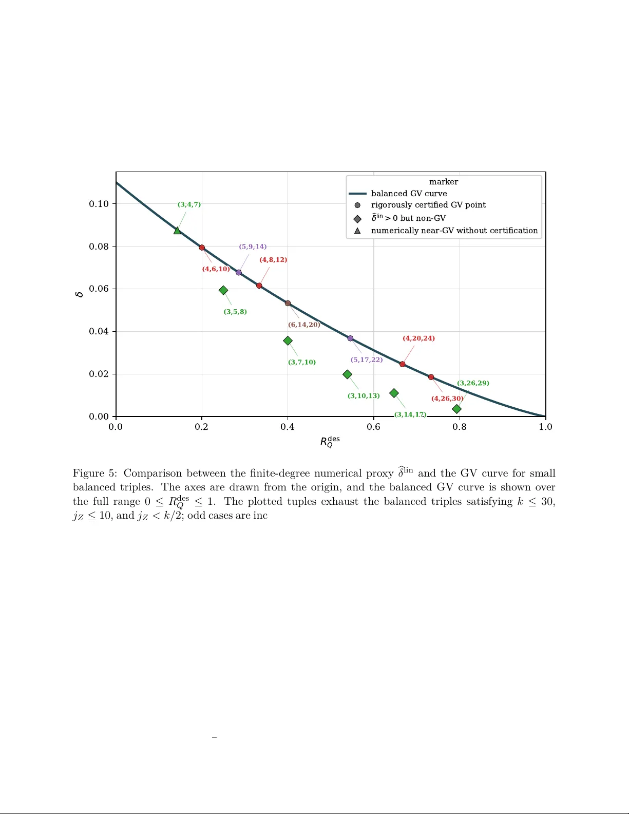
Finite-Degree Quan tum LDPC Co des Reac hing the Gilb ert–V arshamo v Bound Ken ta Kasai Institute of Science T oky o kenta@ict.eng.isct.ac.jp Abstract W e construct nested Calderbank–Shor–Steane co de pairs with non-v anishing co ding rate from Hsu–Anastasop oulos co des and MacKay–Neal co des. In the xed-degree regime, we prov e relativ e linear distance with high probability . Moreo ver, for several nite degree settings, we pro ve Gilb ert–V arshamov distance by a rigorous computer-assisted pro of. 1 In tro duction F rom the viewp oint of asymptotically go o d Calderbank–Shor–Steane (CSS) low-densit y parity-c heck (LDPC) codes, the h yp ergraph-pro duct construction of Tillic h and Zémor [ 1 ] provided a benchmark family with constant rate and distance d = Θ( √ n ) , and for many y ears this remained a represen ta- tiv e reference p oint. The rst asymptotically go o d quantum LDPC families app eared only recen tly through the lifted-pro duct construction of Pan teleev and Kalac hev [ 2 ] and the Cayley-complex-based construction of Dinur, Hsieh, Lin, and Vidick [ 3 ]. Leverrier and Zémor’s quantum T anner co des [ 4 ] then gav e a particularly transparent T anner-st yle CSS-LDPC realization of this breakthrough, and they now serve as one of the main b enc hmarks in the study of go o d quantum LDPC and CSS- LDPC co des. These breakthroughs, how ever, are primarily about simultaneously achieving rate, distance, and sparsit y , rather than ab out explicit large-girth design. In this sense, recen t work has also emphasized that large-girth design is not automatic under orthogonality constraints [ 5 ]. The minim um-distance analysis of classical LDPC co des also has a long history . The linear minim um-distance prop ert y of regular ensembles goes back to Gallager’s classical work [ 6 ]. Later, Di, Ric hardson, and Urbank e [ 7 ] developed weigh t-distribution and spectral-shap e analysis for irregular ensem bles, and Kasai et al. [ 8 ] extended the same viewp oint to multi-edge type LDPC co des. Clas- sical distance analysis for Hsu–Anastasopoulos co des was also given in [ 9 ]. F or MacKa y–Neal co des, prior distance-analysis results include distance-growth analysis for spatially coupled MacKa y–Neal ensem bles [ 10 ] and input-output enumerator analysis for protograph-based MacKa y–Neal co des [ 11 ]. On the classical side, MacKay–Neal (MN) co des [ 12 ] were introduced as early sparse graph co des with lo w-density parity-c heck representations and p erformance close to the Shannon limit. In con- trast, Hsu–Anastasopoulos (HA) co des [ 9 ] provided co de families that retain b ounded graphical complexit y while ac hieving capacit y on memoryless binary-input symmetric-output channels under maxim um-likelihoo d deco ding. The spatially coupled MacKa y–Neal (SC-MN) and spatially coupled Hsu–Anastasop oulos (SC-HA) families were then prop osed in [ 13 ], and b ounded-degree spatial cou- pling is known to ac hieve c hannel capacit y on the binary erasure channel (BEC) [ 14 ]. F or SC-MN / SC-HA families, n umerical threshold analysis on the additive white Gaussian noise c hannel also 1 indicates that the estimated b elief-propagation (BP) threshold approaches the Shannon limit [ 10 ], and universalit y ov er generalized erasure channels with memory has also b een discussed [ 15 ]. It is also kno wn that HA and MN co des are dual to eac h other [ 13 ]. In this pap er, w e do not use this dual pair as is. Instead, we imp ose a nested structure on the MN side and thereb y obtain a sparse CSS code pair. Indeed, if R denotes the classical rate of C , then using an exact dual pair C and C ⊥ directly as a CSS pair giv es the quan tum rate R Q = R + (1 − R ) − 1 = 0 . Thus, obtaining the non-v anishing coding rate sought here requires a non trivial nested structure rather than direct dual pairing. More concretely , we in tro duce a balanced regular MN/HA family whose classical design rates are matched while a p ositive design quan tum rate is retained. As the underlying ensemble, we adopt the sock et-based random graph ensemble of [ 16 , Secs. 3.3–3.4], b oth for the distance analysis in the present pap er and with a view tow ard future densit y-evolution analysis [ 16 , Sec. 3.9 and App. B]. W e study the minimum-distance prop erties of this family . On the HA side, the pro of follows [ 9 ]. Ho wev er, the ensemble considered here is not literally iden tical to that of [ 9 ]: there the outer co de is drawn from a Gallager ensem ble, whereas here w e use the so c ket-based conguration model. W e therefore replace only the small-supp ort and complement estimates by lemmas appropriate for the presen t ensemble. On the MN side, by con trast, the nested structure turns the relev ant parit y-c heck matrix in to a stack ed ob ject that is no longer a standard regular ensemble. This requires a mo died exact-en umerator analysis. Our results are as follows. First, at xed degrees, b oth classical constituent co des ha ve linear minim um distance. Second, for sev eral explicit nite balanced triples, b oth classical constituen t co des attain Gilbert–V arshamov (GV) distance already at nite degree, b y a rigorous computer- assisted pro of. Third, w e show that these nite triples also attain the CSS Gilb ert–V arshamo v distance corresponding to the CSS existence results of Calderbank–Shor and Steane [ 17 , 18 ]. The remainder of this paper is organized as follows. Section 2 presen ts the general framework of the prop osed construction and its regular sparse sp ecialization, together with the design rates and basic prop erties. Sections 3 and 4 give, resp ectively on the Hsu–Anastasop oulos side and on the MacKa y–Neal side, b oth the xed-degree distance analysis and nite-degree GV theorems for sev eral explicit balanced triples. Section 5 com bines these ingredients to ev aluate the relative linear distance of the nested CSS pair and its nite-degree attainment of the CSS Gilb ert–V arshamo v distance. Section 6 presents parameter examples for balanced regular triples. Section 7 concludes the pap er. The app endices contain the deferred Hsu–Anastasop oulos-side and MacKa y–Neal-side pro ofs, the details of the nite-degree certication, and the pro of of probabilistic conv ergence of the actual rates to the design rates. 2 Construction and Basic Prop erties W e work o ver the binary eld F 2 . Ker M denotes the k ernel of a matrix M , and Row( M ) its row space. The binary entrop y function is h 2 ( x ) := − x log 2 x − (1 − x ) log 2 (1 − x ) for 0 < x < 1 . This section rst gives in Section 2.1 the general framew ork of the prop osed co de pair under the sole nested assumption Ro w( A Z ) ⊆ Row( A X ) for arbitrary matrices A Z , A X , B , together with the CSS condition and the dimension formulas for the actual rates. Section 2.2 then sp ecializes this framew ork to regular LDPC matrices and a square regular sparse map. Section 2.3 states the design rates, the balanced condition, and an illustrative concrete example. Finally , Section 2.4 explains ho w to represent compressed syndromes b y sparse ane systems. 2 2.1 General Denition Denition 2.1 (General F ramew ork of the Prop osed Construction) . Let A Z ∈ F m Z × n 2 , A X ∈ F m X × n 2 , and B ∈ F n × n 2 b e arbitrary matrices satisfying Row( A Z ) ⊆ Ro w ( A X ) . F or example, this condition is automatically satised if A Z is c hosen as a row submatrix of A X . In what follows, the righ tmost n co ordinates corresp ond to the visible v ariable v ∈ F n 2 , while the left blo ck corresp onds to hidden v ariables. More precisely , the left blo ck is u ∈ F n 2 for H ′ Z and w ∈ F m X 2 for H ′ X . Dene the extended parity-c heck matrices with hidden v ariables b y H ′ Z :=  A Z 0 B I n  , H ′ X :=  A T X B T  The relev ant co des C Z and C X are obtained b y puncturing the left hidden-v ariable part of Ker H ′ Z and Ker H ′ X , respectively . Concretely , C Z = { v ∈ F n 2 : ∃ u ∈ F n 2 , H ′ Z ( u , v ) T = 0 } and C X = { v ∈ F n 2 : ∃ w ∈ F m X 2 , H ′ X ( w , v ) T = 0 } dene the Z-side and X-side codes. In what follows, esp ecially when w e sp ecialize to regular sparse families, these matrices are sam- pled according to the sock et-based random graph ensem ble of [ 16 , Secs. 3.3–3.4]. This c hoice is natural for the exact-enumerator analysis carried out here and is also consistent with future deco d- ing analyses based on density evolution [ 16 , Sec. 3.9 and App. B]. This hidden-v ariable represen tation immediately yields the reduced forms used later in the anal- ysis: C Z = B (Ker A Z ) , C Z ( A X ) := B (Ker A X ) , and C X = { v ∈ F n 2 : ∃ w , A T X w + B T v = 0 } . Indeed, H ′ Z ( u , v ) T = 0 is equiv alent to A Z u = 0 and v = B u , while H ′ X ( w , v ) T = 0 is equiv alent to A T X w + B T v = 0 . The auxiliary co de C Z ( A X ) , used later, is obtained from the Z-side expression for C Z b y replacing A Z with A X . Theorem 2.2 (Nested CSS pair) . Under Denition 2.1 , C ⊥ Z ⊆ C X holds. In particular, ( C X , C Z ) forms a CSS pair. Pr o of. F or an y subspace U ⊆ F n 2 , v ∈ ( B U ) ⊥ ⇐ ⇒ h v , B u i = 0 ∀ u ∈ U ⇐ ⇒ h B T v , u i = 0 ∀ u ∈ U ⇐ ⇒ B T v ∈ U ⊥ . First, C ⊥ Z = { v ∈ F n 2 : B T v ∈ (Ker A Z ) ⊥ = Ro w ( A Z ) } , and similarly  C Z ( A X )  ⊥ = { v ∈ F n 2 : B T v ∈ (Ker A X ) ⊥ = Ro w ( A X ) } = C X . The last equality holds b ecause B T v ∈ Row( A X ) can b e written as A T X w + B T v = 0 for some w . On the other hand, Row( A Z ) ⊆ Row( A X ) implies Ker A X ⊆ Ker A Z , so C Z ( A X ) = B (Ker A X ) ⊆ B (Ker A Z ) = C Z . T aking orthogonal complements giv es C ⊥ Z ⊆  C Z ( A X )  ⊥ = C X as claimed. Denition 2.3 (Compressed parity-c heck matrices) . F or the general framew ork of Denition 2.1 , let Row( H Z ) = C ⊥ Z and Row( H X ) = C ⊥ X , and call an y visible-v ariable matrices H Z ∈ F r Z × n 2 and H X ∈ F r X × n 2 compressed parity-c heck matrices for C Z and C X , resp ectiv ely , if they satisfy these ro w-space conditions. By the pro of of Theorem 2.2 , one ma y take Row( H Z ) = { v ∈ F n 2 : ∃ x ∈ F m Z 2 , A T Z x + B T v = 0 } and Row( H X ) = C Z ( A X ) = B (Ker A X ) . In particular, if K X is a basis matrix of Ker A X , then H X = K X B T is one p ossible c hoice of H X , and a basis of the kernel of [ A T Z B T ] , projected to the visible comp onen t, gives one p ossible c hoice of H Z . These matrices are not unique in general; dierent row-equiv alen t representativ es dene the same co de. T o distinguish them from the design rates in tro duced later, we call the following quantities the actual co ding rates: R Z := dim C Z n , R X := dim C X n , and R Q := R X + R Z − 1 , where R Q is the quan tum rate. 3 Prop osition 2.4 (Dimension formulas for the actual rates) . L Z := dim(Ker A Z ∩ Ker B ) and L X := dim(Ker A X ∩ Ker B ) . Then R Z = n − rank A Z − L Z n , R X = rank A X + L X n , R Q = rank A X − rank A Z + L X − L Z n , and moreo ver L X ≤ L Z holds. Pr o of. By the rank-nullit y formula for the image of a linear map, dim C Z = dim B (Ker A Z ) = dim Ker A Z − dim(Ker A Z ∩ Ker B ) = n − rank A Z − L Z , which yields R Z = n − rank A Z − L Z n for the Z-side rate. Also, C X =  B (Ker A X )  ⊥ , so dim C X = n − dim B (Ker A X ) = n − ( n − rank A X − L X ) = rank A X + L X , and therefore R X = rank A X + L X n follo ws. Hence R Q = R X + R Z − 1 = rank A X − rank A Z + L X − L Z n as stated. Finally , Ker A X ⊆ Ker A Z implies Ker A X ∩ Ker B ⊆ Ker A Z ∩ Ker B , and hence L X ≤ L Z . 2.2 Denition Using LDPC Matrices In this subsection, w e sp ecialize the general framework of Section 2.1 to a family dened b y regular sparse matrices. Denition 2.5 (Nested regular sparse family) . The regular sparse sp ecialization of the general framew ork in Denition 2.1 is dened as follo ws. T ake positive integers k, j Z , j X , k Z , k ∆ suc h that 1 ≤ j Z < j X , and set j ∆ := j X − j Z . Let m Z , m ∆ , m X denote the n umbers of rows of A Z , A ∆ , A X , resp ectively . First sample A Z ∈ F m Z × n 2 from the standard ( j Z , k Z ) -regular LDPC ensemble [ 16 , Secs. 3.3–3.4]. Next sample A ∆ ∈ F m ∆ × n 2 indep enden tly from the standard ( j ∆ , k ∆ ) -regular LDPC ensem ble, and dene A X :=  A Z A ∆  ∈ F m X × n 2 and m X := m Z + m ∆ . In a regular T anner graph, the num b er of edges on the v ariable-no de side must agree with that on the c heck-node side, so j Z n = k Z m Z and j ∆ n = k ∆ m ∆ m ust hold. In particular, m Z = j Z k Z n and m ∆ = j ∆ k ∆ n follow. Throughout we assume k Z | j Z n and k ∆ | j ∆ n so that these quantities are in tegers. Finally , sample B ∈ F n × n 2 indep enden tly from the square ( k , k ) -regular sparse ensemble [ 16 , Secs. 3.3–3.4]. Since A X = [ A Z ; A ∆ ] , the inclusion Row( A Z ) ⊆ Row( A X ) holds automatically , and Denition 2.1 therefore gives a nested CSS pair ( C X , C Z ) . F rom this p oint on, the stac ked matrix A X = [ A Z ; A ∆ ] itself is treated as the object of analysis, without replacing it by a homogeneous regular ensemble. In this pap er, the “standard ( j, k ) -regular LDPC ensemble” means the regular ensem ble obtained from the so ck et-based conguration mo del of [ 16 , Secs. 3.3–3.4], with optional conditioning on the simple-graph even t when needed. Lik e- wise, the “square ( k , k ) -regular ensem ble” means the square regular case of the same conguration mo del. That is, one assigns j (or k ) so ck ets to eac h column-side no de, k (or j ) so ck ets to eac h ro w-side no de, and then forms the T anner graph by a uniformly random p erfect matching. The co ecien t-extraction form ulas and pairing b ounds below are derived rst as exact statemen ts for the unconditioned conguration mo del, which allo ws m ultiple edges. On the other hand, for xed degrees, the simple-graph even t has probabilit y b ounded aw ay from zero as n → ∞ , so the o (1) rst-momen t b ounds and negative exp onen tial upp er b ounds prov ed in the unconditioned mo del transfer unc hanged to the conditioned simple ensemble. Hence the asymptotic claims on distance and rate are justied for the F 2 -v alued regular matrix ensem bles used in the main text. 4 2.3 Design Rates and Balanced Conditions Denition 2.6 (Design rates) . The design rates are the rates determined purely by the degrees, obtained from the actual-rate form ulas in Prop osition 2.4 by formally discarding the nite-length con tributions of rank deciency and k ernel ov erlap. Namely , substitute rank A Z = m Z , rank A X = m X , and L Z = L X = 0 in to the form ulas, and dene R des Z := ( n − m Z ) /n and R des X := m X /n . F or even k , Prop osition C.3 in App endix C sho ws that B 1 [ n ] = 0 , so rank B = n nev er o ccurs at nite blo cklength. Nevertheless, dim Ker B = o ( n ) holds with high probabilit y , so this design rate agrees with the asymptotic v alue of the actual rate. Prop osition 2.7 (F orm ula for the design quan tum rate) . R des Q = R des X + R des Z − 1 = ( m X − m Z ) /n = m ∆ /n = j ∆ /k ∆ holds. Pr o of. By Denitions 2.6 and 2.5 , R des X = m X /n = ( m Z + m ∆ ) /n = j Z /k Z + j ∆ /k ∆ and R des Z = ( n − m Z ) /n = 1 − j Z /k Z . Hence R des X + R des Z − 1 = m X /n + ( n − m Z ) /n − 1 = ( m X − m Z ) /n = m ∆ /n = j ∆ /k ∆ . The necessary and sucient condition for the tw o classical design rates to coincide is R des X = R des Z ⇐ ⇒ m X /n = 1 − m Z /n ⇐ ⇒ m X + m Z = n ⇐ ⇒ 2 j Z /k Z + j ∆ /k ∆ = 1 , and we call this the general balanced condition. Example 2.8 (An illustrativ e example of the general balanced condition) . T o illustrate the general balanced condition concretely , consider the example n = 40 , m Z = 15 , m ∆ = 10 , and m X = 25 , with degrees ( j Z , k Z , j ∆ , k ∆ , k ) = (3 , 8 , 2 , 8 , 2) . Then m Z = (3 / 8) n , m ∆ = (2 / 8) n , and m X = (5 / 8) n , so m X + m Z = n indeed holds. On the other hand, since k Z = k ∆ = 8 whereas k = 2 , this example do es not b elong to the homogeneous sp ecialization introduced immediately b elow. Accordingly , Figures 1 and 2 visualize a stack ed blo c k structure already permitted at the lev el of the general balanced condition. F or the same example, Figures 3 and 4 show compressed parity-c heck matrices H Z , H X obtained without taking reduced row ec helon form (RREF). Here H Z is obtained b y pro jecting a basis of the k ernel of [ A T Z B T ] to the visible comp onent, and H X is dened from a basis matrix K X of Ker( A X ) b y H X = K X B T . No nal ro w-reduction b y elemen tary row op erations is applied to either visible matrix. F or this generated example, w e also veried directly ov er F 2 that H X H T Z = 0 holds. The design rates are R des Z = ( n − m Z ) /n = 25 / 40 = 0 . 625 , R des X = m X /n = 25 / 40 = 0 . 625 , and R des Q = m ∆ /n = 10 / 40 = 0 . 25 . On the other hand, for the generated matrices w e ha ve rank H Z = 16 and rank H X = 15 , so R Z = dim C Z /n = (40 − 16) / 40 = 24 / 40 = 0 . 6 , R X = dim C X /n = (40 − 15) / 40 = 25 / 40 = 0 . 625 , and R Q = (dim C X + dim C Z − n ) /n = (25 + 24 − 40) / 40 = 9 / 40 = 0 . 225 . Th us, in this nite-length example, R X agrees with its design v alue, while R Z and R Q are sligh tly smaller because of nite-length rank deciency . In the distance analysis below, w e assume the homogeneous sp ecialization k Z = k ∆ = k . This assumption is made in order to simplify the co ecient-extraction formulas and symmetry statemen ts used in the xed-degree analysis from Section 3 onw ard and in the nite-degree GV theorems for explicit triples. That is, the rst half of Section 2 denes the stac ked family with general ( j Z , k Z ) and ( j ∆ , k ∆ ) -regular blocks, and from this p oin t on w e restrict atten tion to the homogeneous sub class in whic h the row degree is also common. Since j ∆ = j X − j Z , the balanced condition then reduces 5 Figure 1: Z-side extended parity-c heck matrix for the illustrative example ( j Z , k Z , j ∆ , k ∆ , k ) = (3 , 8 , 2 , 8 , 2) , n = 40 , m Z = 15 , and m ∆ = 10 (hence m X = 25 ): H ′ Z =  A Z 0 B I n  ∈ F 55 × 80 2 . The blue blo c k in the upp er left is the (3 , 8) -regular matrix A Z ∈ F 15 × 40 2 , the light-blue block in the lo wer left is the square (2 , 2) -regular sparse map B ∈ F 40 × 40 2 , the y ellow blo ck in the lo wer right represen ts I n , and the upp er-right blo ck is zero. Black lines indicate blo ck b oundaries. to j X + j Z = k , and from no w on w e assume this homogeneous balanced condition and call an y suc h parameter triple ( j Z , j X , k ) a balanced triple. In this case R des Z = R des X = j X k = 1 − j Z k and R des Q = j ∆ k = 1 − 2 j Z k > 0 hold. Note that the low er b ound 4 ≤ j Z is not needed to dene the nested CSS pair itself; it is imp osed only later in the xed-degree distance analysis. The next theorem states that the design rates introduced here are not merely formal proxies: they asymptotically describ e the actual rates of the nite-length codes. Its signicance is that the distance analysis b elow may therefore use the ratios determined by the design rates without losing con tact with the asymptotic parameters of the actual co de family . In what follows, w e assume the homogeneous sp ecialization k Z = k ∆ = k together with a xed ev en balanced triple satisfying 4 ≤ j Z < k 2 , j Z ≡ 0 (mo d 2) , and j X − j Z ≡ 0 (mo d 2) . The lemmas and pro ofs needed for the next theorem are deferred to Appendix C . Theorem 2.9 (The actual rates con verge in probabilit y to the design rates) . R Z → R des Z = j X k , R X → R des X = j X k , and R Q → R des Q = j X − j Z k hold as conv ergence in probabilit y when n → ∞ . 6 Figure 2: X-side extended parity-c heck matrix for the same example: H ′ X = [ A T X B T ] = [ A T Z A T ∆ B T ] ∈ F 40 × 65 2 . F rom left to right, the blue blo c k is the (3 , 8) -regular matrix A T Z ∈ F 40 × 15 2 , the red block is the (2 , 8) -regular matrix A T ∆ ∈ F 40 × 10 2 , and the light-blue blo ck is B T ∈ F 40 × 40 2 . Th us the stack ed structure of A X = [ A Z ; A ∆ ] ∈ F 25 × 40 2 is visualized directly . Blac k lines indicate blo c k b oundaries. A ccordingly , in the distance analysis below, the natural reference quantities are the ratios deter- mined b y the design rates, rather than nite-length rank deciencies. 2.4 Sparse-Matrix Represen tation of Syndrome Consistency In this subsection, w e use the sparse extended matrices H ′ Z and H ′ X in tro duced in Section 2.2 to rewrite the decoding conditions for the compressed syndromes as ane sparse systems. This also mak es explicit that the present family has bounded graphical complexit y and admits BP implemen- tations with linear p er-iteration complexity . F or the nested regular sparse family , the n umbers of edges in the T anner graphs of H ′ Z and H ′ X in tro duced in Denition 2.1 are j Z n + k n + n and j X n + k n , respectively . If j Z , j X , k Z , k ∆ , k are xed, b oth are O ( n ) . Therefore the presen t family has b ounded graphical complexit y in the sense of [ 9 ]. Although the compressed-syndrome matrices H Z , H X are generally dense, syndrome decoding asks us to estimate noise vectors e X , e Z from the measured syndromes s Z , s X under the compressed syndrome equations H Z e X = s Z and H X e Z = s X . Once a syndrome representativ e is injected, this deco ding scenario can still b e represen ted by ane sparse systems that retain the sparse structure of H ′ Z and H ′ X . 7 Figure 3: Z-side compressed parity-c hec k matrix for the same example: H Z ∈ F 16 × 40 2 . It is obtained b y pro jecting a basis of the k ernel of [ A T Z B T ] to the visible comp onent, without taking RREF on the nal visible matrix. Thus each row represents an explicit generator of C ⊥ Z . Figure 4: X-side compressed parit y-chec k matrix for the same example: H X ∈ F 16 × 40 2 . If K X is a basis matrix of Ker( A X ) , then this gure displa ys H X = K X B T directly , again without taking RREF on the nal visible matrix. Thus each row represents an explicit generator of C ⊥ X . In what follows, let H Z b e a full-row-rank compressed parit y-chec k matrix in the sense of Deni- tion 2.3 , and let K X b e a full-ro w-rank basis matrix of Ker A X . On the Z side, x any right inv erse Γ Z satisfying H Z Γ Z = I . On the X side, take the compressed representativ e H X := K X B T and x an y right inv erse Γ X satisfying K X Γ X = I . W rite t Z := Γ Z s Z and t X := Γ X s X . Theorem 2.10 (Sparse ane representations of the syndrome equations) . The syndrome equations H Z e X = s Z and H X e Z = s X hold if and only if there exist f X ∈ F n 2 on the Z side and f Z ∈ F m X 2 on the X side such that  A Z 0 B I n   f X e X  =  0 t Z  and  A T X B T   f Z e Z  = t X . Equiv alently , A Z f X = 0 , e X = t Z + B f X , and B T e Z = t X + A T X f Z hold sim ultaneously . Pr o of. On the Z side, A Z f X = 0 and e X = t Z + B f X imply B f X ∈ B (Ker A Z ) = C Z , and Row( H Z ) = C ⊥ Z therefore gives H Z ( B f X ) = 0 . Hence H Z e X = H Z ( t Z + B f X ) = H Z t Z = H Z Γ Z s Z = s Z . Con versely , H Z e X = s Z implies H Z ( e X − t Z ) = 0 , so e X − t Z ∈ Ker H Z = C Z = B (Ker A Z ) , and th us there exists f X ∈ Ker A Z suc h that e X = t Z + B f X . On the X side, B T e Z = t X + A T X f Z implies K X B T e Z = K X t X = K X Γ X s X = s X b ecause K X A T X = 0 . Since H X := K X B T , this is exactly H X e Z = s X . Conv ersely , H X e Z = s X implies 8 K X ( B T e Z − t X ) = 0 . The row space of K X is Ker A X , so its right kernel equals Row( A X ) . Therefore there exists f Z ∈ F m X 2 suc h that B T e Z − t X = A T X f Z , namely B T e Z = t X + A T X f Z . The sparse matrices app earing here are exactly  A Z 0 B I n  = H ′ Z and  A T X B T  = H ′ X . Hence, in the nested regular sparse family , their num b ers of nonzero entries are j Z n + k n + n and j X n + k n , resp ectiv ely , and running BP on the corresp onding T anner graphs requires O ( n ) op erations p er iteration. Ho wev er, the sparse object here is the matrix represen tation of the ane systems after the rep- resen tatives t Z , t X ha ve been injected externally . The step that forms t Z , t X from the compressed syndromes is still generally dense. Moreov er, in these T anner graphs ev ery c heck no de is adjacen t to multiple punctured no des f X or f Z , so xing the syndrome bits do es not by itself pro duce non- trivial BP messages on the visible v ariables e X , e Z at the initial up date. Thus this theorem should b e read as giving a sparse ane representation for a xed syndrome representativ e, not a sparse measuremen t matrix for the compressed syndromes themselves or a directly usable BP deco der. 3 Distance Analysis on the Hsu–Anastasop oulos Side This section states the distance results on the HA side. F or xed degrees, a p ositive linear distance follo ws from a lo w-output-weigh t argument. Although in Section 2 we did not dene C Z = B (Ker A Z ) as a concatenated co de, the analysis in this section views it in that w a y: Ker A Z pla ys the role of the outer co de, and the map u 7→ B u is the inner regular sparse map. That is, w e rst c ho ose an outer co deword u ∈ Ker A Z , and then obtain v = B u through the inner map B . The proof throughout this section follo ws the HA-side analysis in [ 9 ]. How ever, the ensemble itself is not the same: in [ 9 ] the outer co de is a Gallager ensem ble, whereas here b oth the inner and outer parts are modeled by the so ck et-based conguration mo del of [ 16 , Secs. 3.3–3.4]. F or this reason, w e state only the results in the main text, and mo ve to App endix A the transition en umerator, the rst-moment estimates, and the proof of the xed-degree theorem, namely the parts of the argumen t in [ 9 ] that m ust b e rewritten for the present ensemble. Theorem 3.1 (Fixed-degree positive linear distance on the HA side) . Assume a xed ev en balanced triple satisfying 4 ≤ j Z < k 2 , j Z ≡ 0 (mod 2) , and j ∆ := j X − j Z ≡ 0 (mod 2) . Then there exists a constan t δ lin Z > 0 , dep ending only on ( j Z , k ) , such that for every 0 < δ < δ lin Z , P [ d ( C Z ) ≤ δ n ] → 0 ( n → ∞ ) holds. In particular, d ( C Z ) = Ω( n ) holds with high probability . Here the classical Gilb ert–V arshamo v (GV) distance for binary linear co des is the existence curve R ≥ 1 − h 2 ( δ ) , or equiv alently δ GV ( R ) = h − 1 2 (1 − R ) , as given in [ 19 , 20 ]. The design rate of the HA-side constituen t co de C Z considered here is R des Z = α X = 1 − α Z , so the corresp onding classical GV point is δ GV ( R des Z ) = h − 1 2 (1 − α X ) = h − 1 2 ( α Z ) . Let the searc h windo w b e T scan := { ( j Z , j X , k ) : k ≤ 30 , j Z ≤ 10 , j Z < k / 2 , j X = k − j Z } . Here w e restrict attention to this lo w-degree region in order to examine nite-degree GV attain- men t while keeping the degrees gen uinely small. This is the full set of balanced triples scanned exhaustiv ely for the nite-degree certication and for Fig. 5 . Let T GV := { (4 , 6 , 10) , (4 , 8 , 12) , (5 , 9 , 14) , (6 , 14 , 20) , (5 , 17 , 22) , (4 , 20 , 24) , (4 , 26 , 30) } ⊂ T scan denote the balanced triples in this searc h window for which the nite-degree certication of App en- dices D and E closes rigorously . These are exactly the circular markers in Fig. 5 . 9 Theorem 3.2 (Finite-degree GV attainment on the HA side) . F or eac h ( j Z , j X , k ) ∈ T GV , let δ GV := δ GV ( R des Z ) = h − 1 2 (1 − R des Z ) . Then for ev ery 0 < δ < δ GV , P [ d ( C Z ) ≤ δ n ] → 0 ( n → ∞ ) holds. In this sense, ev ery triple in T GV attains the classical GV p oin t on the HA side at nite degree. Pr o of. The pro of is deferred to App endix D . W e also stress that [ 9 , Theorem 2 and Corollary 1] do es not pro ve a nite-degree GV statemen t of the form ab ov e for each xed triple. More precisely , its result is an ε – K large-degree statement: for an y ε > 0 , there exists a sucien tly large integer K ( ε ) such that whenev er k ≥ K ( ε ) , the normalized minim um distance can be made within ε of the GV b ound. Equiv alently , [ 9 ] sho ws approach to the GV b ound in the limit k → ∞ , rather than nite-degree GV attainmen t for each xed triple as in the theorem ab o ve. 4 Distance Analysis on the MacKa y–Neal Side W e now turn to the MN side. The imp ortant p oint is that the actual mo del is A X =  A Z A ∆  , namely a stack ed ensemble, not a standard ( j X , k ) -regular ensemble. The multi-edge type low- densit y parity-c heck framew ork of [ 8 ], the SC-MN w eight-en umerator analysis of [ 10 ], and the protograph-based MN input-output en umerator analysis of [ 11 ] are close in spirit to this section, but none of them studies the stack ed ensemble treated here itself. Accordingly , one m ust build, on this stac ked ensem ble itself, the stack ed rened en umerator, the exact conguration form ula, the blo ckwise complemen t symmetry coming from ev en degrees, the trial-point b ounds gov erning the linear-w eight regime, and the pairing bound gov erning the lo w-weigh t regime. W e defer these details, as well as the pro of of the xed-degree theorem, to App endix B , and state only the t wo resulting theorems in this section. Theorem 4.1 (Fixed-degree p ositive linear distance on the MN side) . Assume a xed nite bal- anced triple satisfying 4 ≤ j Z < k 2 , j Z ≡ 0 (mod 2) , and j ∆ := j X − j Z ≡ 0 (mod 2) . Then there exists a constan t δ lin X > 0 such that for ev ery 0 < δ < δ lin X , one has P [ d ( C X ) ≤ δ n ] → 0 as n → ∞ . In particular, d ( C X ) = Ω( n ) holds with high probability . Pr o of. The pro of is deferred to App endix B . The nite-degree GV proof k eeps the same low-w eight / linear-w eight decomp osition, and the remaining nite-domain chec ks are closed in App endix E by explicit b ox upp er b ounds. Theorem 4.2 (Finite-degree GV attainmen t on the MN side) . F or eac h ( j Z , j X , k ) ∈ T GV , dene δ GV := δ GV ( R des X ) = h − 1 2 (1 − R des X ) . Then for ev ery 0 < δ < δ GV , P [ d ( C X ) ≤ δ n ] → 0 as n → ∞ . In this sense, every triple in T GV attains the classical GV p oint on the MN side at nite degree. Pr o of. The pro of is deferred to App endix E . 10 5 Relativ e Distance of the Nested CSS P air Dene the relative distances of the nested CSS pair ( C X , C Z ) , with the conv en tion that the v alue is + ∞ when the corresp onding dierence set is empty , by d rel Z := min { wt( v ) : v ∈ C Z \ C Z ( A X ) } and d rel X := min { wt( v ) : v ∈ C X \ C ⊥ Z } . Corollary 5.1 (Relativ e linear distance for xed even degrees) . Assume a xed even balanced triple satisfying 4 ≤ j Z < k 2 , j Z ≡ 0 (mo d 2) , and j X − j Z ≡ 0 (mo d 2) . Then the nested CSS pair has relative linear distance. That is, there exist δ lin Z , δ lin X > 0 such that for every 0 < δ Z < δ lin Z and 0 < δ X < δ lin X , one has P [ d rel Z ≤ δ Z n ] → 0 and P [ d rel X ≤ δ X n ] → 0 . Pr o of. F rom C Z ( A X ) ⊆ C Z and C ⊥ Z ⊆ C X , we obtain C Z \ C Z ( A X ) ⊆ C Z \ { 0 } and C X \ C ⊥ Z ⊆ C X \ { 0 } . Hence d rel Z ≥ d ( C Z ) and d rel X ≥ d ( C X ) , and Theorems 3.1 and 4.1 nish the pro of. Under the balanced condition, the quantum design rate is R des Q = 1 − 2 α Z . On the other hand, the asymptotic existence b ound corresponding to the CSS existence results of Calderbank–Shor and Steane is R Q ≥ 1 − 2 h 2 ( δ ) , or equiv alently δ CSS - GV ( R Q ) = h − 1 2  1 − R Q 2  , as given in [ 17 , 18 ]. Therefore, for a nite triple ( j Z , j X , k ) , the target v alue is δ CSS - GV ( R des Q ) = h − 1 2  1 − (1 − 2 j Z /k ) 2  = h − 1 2  j Z k  . Th us the t wo theorems ab o ve imply that this v alue is attained already at nite degree for ev ery triple in T GV . Corollary 5.2 (Balanced triples attaining the CSS Gilb ert–V arshamov distance at nite degree) . F or eac h ( j Z , j X , k ) ∈ T GV , let δ GV := δ CSS - GV ( R des Q ) = h − 1 2  1 − R des Q 2  . Then for ev ery 0 < δ < δ GV , P [ d rel Z ≤ δ n ] → 0 and P [ d rel X ≤ δ n ] → 0 ( n → ∞ ) hold. In this sense, ev ery triple in T GV attains the CSS Gilbert–V arshamov distance at nite degree. Pr o of. This follows immediately from Theorems 3.2 and 4.2 together with d rel Z ≥ d ( C Z ) and d rel X ≥ d ( C X ) . 6 P arameter Examples of Balanced Regular T riples This section illustrates numerically the nite-degree b ehavior of balanced regular triples. Since the gures also include o dd balanced triples, they should be read as supplemen tary plots of nite-degree pro xies rather than theorem statements. Instead of the existen tial constants δ lin Z , δ lin X app earing in the xed-degree theorems, w e compare n umerical pro xies at nite degree. Let b δ lin Z b e the rightmost zero of the visible upp er env elop e W ub Z ( ω ) from Section 3, and let b δ lin X b e the righ tmost zero of the visible X-side en velope obtained from the MN-side trial-point bound ( 12 ). Set b δ lin := min { b δ lin Z , b δ lin X } . If the corresponding zero do es not exist, we set the proxy to 0 . If m ultiple zeros exist, we choose the largest zero such that the corresp onding en velope is nonp ositive on its immediate left. In this section w e exhaust the searc h window T scan = { ( j Z , j X , k ) : k ≤ 30 , j Z ≤ 10 , j Z < k / 2 , j X = k − j Z } and determine, for eac h triple, whether the rst-moment b ounds from Sections 3 and 4 close rigor- ously with the certied constants of App endices D and E . Figure 5 compares, ov er this search 11 windo w, the nite-degree n umerical proxy b δ lin with the GV curve along the balanced relation α Z = (1 − R des Q ) / 2 . The plot exhausts all balanced triples satisfying k ≤ 30 , j Z ≤ 10 , j Z < k / 2 , and j X = k − j Z . Circular markers are rigorously certied triples, triangular mark ers are numerically near-GV triples without certication, and red p oints are p ositiv e-proxy but non-GV triples. At presen t only (3 , 4 , 7) is sho wn in the triangular category . T uples with b δ lin = 0 are omitted from the gure. Eac h display ed p oin t is lab eled with the corresponding triple ( j Z , j X , k ) . 0.0 0.2 0.4 0.6 0.8 1.0 R d e s Q 0.00 0.02 0.04 0.06 0.08 0.10 marker balanced GV curve rigorously certified GV point l i n > 0 b u t n o n - G V numerically near-GV without certification marker balanced GV curve rigorously certified GV point l i n > 0 b u t n o n - G V numerically near-GV without certification Figure 5: Comparison betw een the nite-degree numerical pro xy b δ lin and the GV curv e for small balanced triples. The axes are dra wn from the origin, and the balanced GV curve is shown ov er the full range 0 ≤ R des Q ≤ 1 . The plotted tuples exhaust the balanced triples satisfying k ≤ 30 , j Z ≤ 10 , and j Z < k / 2 ; o dd cases are included as well. Mark er shapes distinguish rigorously certied nite-degree GV p oints, n umerically near-GV p oin ts without certication, and positive-pro xy but non-GV p oints. T uples with b δ lin = 0 are omitted, and each displa y ed p oin t is lab eled b y its triple ( j Z , j X , k ) . The circular mark ers in the gure corresp ond exactly to the triples in T GV , namely the balanced triples in the search window T scan for whic h the nite-degree certication closes rigorously . Equiv- alen tly , they are the triples co vered b y Theorems 3.2 and 4.2 , and hence by Corollary 5.2 . By con trast, the triangular marker is a plot-only p oin t whose numerical pro xy lies very close to the GV curv e, and it is not part of any theorem claim in the present pap er. Ov er the plotted range k ≤ 30 and j Z ≤ 10 , all balanced triples with j Z = 1 , 2 hav e b δ lin = 0 and are therefore omitted from the gure, while among the displa yed p oints every balanced triple with j Z ≥ 4 lies n umerically on or v ery near the GV curv e and the clearly non-GV p oints occur only at j Z = 3 . This suggests the following conjecture. Conjecture 6.1 (Balanced triples attaining nite-degree GV) . Let ( j Z , j X , k ) be an y balanced triple satisfying 4 ≤ j Z < k 2 and j X = k − j Z . Then the corresp onding HA-side and MN-side 12 classical constituent codes attain Gilb ert–V arshamo v distance already at xed nite degree, and hence the asso ciated nested CSS family attains the CSS Gilb ert–V arshamov distance. 7 Conclusion W e constructed a balanced nested regular CSS family entirely from regular LDPC matrices. This family sim ultaneously has b ounded graphical complexity , equal classical design rates, and a p ositive design quantum rate. The most imp ortant p oint is that the MN-side parit y-chec k matrix is the stac ked matrix A X =  A Z A ∆  , and the pro of must therefore be carried out on this stac ked ensem ble itself. The nal conclusions are tw ofold. F or xed even balanced triples, the nested CSS pair has relativ e linear distance with high probability . Moreo ver, for the seven balanced triples T GV in the searc h window T scan for whic h the nite-degree certication closes rigorously , the classical GV p oint, and hence by Corollary 5.2 the CSS Gilb ert–V arshamo v distance, is rigorously certied already at nite degree. Moreov er, the actual classical and quan tum rates conv erge in probability to the corresp onding design rates. Th us the balanced nested regular MN/HA construction simultaneously realizes b ounded graphical complexit y , a p ositive design quan tum rate, xed-degree relativ e linear distance, and explicit nite-degree GV-certied examples. Another imp ortant p oint is that in this family the three blo c ks A Z , A ∆ , and B can be c hosen indep enden tly , so nite-length design retains the freedom to enlarge the girth of the extended parity- c heck matrices. This is signican t b ecause the main large-distance CSS-LDPC constructions in the literature ha ve primarily focused on the simultaneous ac hievemen t of rate, distance, and sparsit y , while large-girth design is not automatic under orthogonalit y constrain ts [ 2 , 3 , 4 , 5 ]. On the other hand, the uncoupled nested construction studied here is primarily an asymptotic guaran tee on distance and rate, and is not itself optimized as a direct target for standard BP deco ding. In fact, the compressed parity-c hec k matrices H Z , H X that pro vide the visible-v ariable syndromes are generally dense, so syndrome measurement is not yet handled as a sparse graph. Ho wev er, as seen in Section 2.4, once syndrome representativ es t Z , t X are injected externally , the compressed syndrome equations themselves can b e written as sparse ane systems in terms of the sparse extended matrices H ′ Z , H ′ X . What remains unresolved is that the step of forming t Z , t X from the compressed syndromes is generally dense, and that each c heck node is adjacent to m ultiple punctured no des, so this sparse represen tation do es not b y itself yield a directly usable BP rule of the kind employ ed for classical MN/HA co des. Accordingly , this paper still does not propose an ecien t deco ding metho d. Ho wev er, on the classical side, b ounded-degree spatial coupling achiev es capacity on the BEC for m ulti-edge type LDPC ensem bles [ 14 ], and for the SC-MN / SC-HA family it is known to impro ve the BP threshold on the BEC [ 13 ], to preserve distance growth [ 10 ], and even to ac hieve universal symmetric information rate on generalized erasure c hannels with memory [ 15 ]. On the quan tum side as well, spatially coupled quasi-cyclic quantum LDPC-CSS co des were prop osed early on in [ 21 ], and there are no w results sho wing sparse-structure deco ding p erformance approac hing the co ding-theoretical b ound [ 22 ], as well as design principles that simultaneously realize regularit y and large girth [ 5 ]. This is a plausible direction rather than a consequence of the presen t analysis. It is therefore natural to exp ect that introducing a spatially coupled version of the nested family studied here could alleviate the issues ab ov e, just as in the classical case, and p ossibly 13 lead to BP-type deco ding rules with near-optimal decoding p erformance. App endix A Pro ofs of the HA-Side Theorems In this app endix we collect the pro of of the HA-side xed-degree theorem omitted from Section 3. The basic pro of structure follo ws [ 9 ]. Ho w ever, here b oth the inner and outer parts are modeled b y the so ck et-based conguration model of [ 16 , Secs. 3.3–3.4], so the needed inputs are restated as lemmas for the present ensemble. A.1 Lemmas and A uxiliary Results Let the av erage weigh t distribution of the outer regular co de Ker A Z b e N o ( s ) := E   { u ∈ Ker A Z : wt( u ) = s }   =  n s   x j Z s   (1+ x ) k +(1 − x ) k 2  m Z  nj Z j Z s  . This count is a rewriting, in the sock et-based notation used here, of the Di–Richardson–Urbank e activ e-edge argumen t [ 7 ] for the av erage weigh t distribution of the regular LDPC ensem ble. Here a so c ket means a half-edge in the conguration model, and an activ e so ck et is the analogue of an active edge in [ 7 ], namely a so c ket emanating from a column that b elongs to a xed supp ort U . Thus the en umeration ab o ve counts, for a xed candidate supp ort U of w eight s , the n umber of congurations in which the j Z s active sock ets are distributed so that each ro w receiv es an ev en n umber of them. Indeed, xing U ⊂ [ n ] with | U | = s , the active column-side sock ets attac hed to U n umber exactly j Z s . Exactly as in the activ e-edge counting of Di–Richardson–Urbank e, under the so ck et-based conguration mo del their images form a uniformly random j Z s -subset of the nj Z = k m Z ro w-side so c kets. The condition that eac h row receiv es an ev en n umber of active sock ets is equiv alent to A Z 1 U = 0 , and since the one-ro w generating function is  (1 + x ) k + (1 − x ) k  / 2 , the co ecient extraction ab ov e giv es the probability that the xed U is a codeword supp ort. Multiplying by the n umber  n s  of supports of size s yields the display ed closed form. In the xed-degree part of this app endix, w e abbreviate α Z := j Z k . W riting s = τ n , w e obtain the standard regular-LDPC exp onent b ound W o ( τ ) := lim sup n →∞ 1 n log 2 N o ( τ n ) ≤ α Z inf x> 0 log 2 (1 + x ) k + (1 − x ) k 2 x τ k − ( j Z − 1) h 2 ( τ ) . (1) This follo ws b y applying the co ecient-extraction b ound [ x j Z s ] F ( x ) ≤ F ( x ) /x j Z s to the closed form ab o ve for an y x > 0 , and then using Stirling’s formula 1 n log 2  n τ n  = h 2 ( τ ) + o (1) , 1 n log 2  nj Z τ nj Z  = j Z h 2 ( τ ) + o (1) . Indeed, 1 n log 2 N o ( τ n ) is b ounded ab ov e b y h ( τ ) + α Z log 2  ((1 + x ) k + (1 − x ) k ) / 2 x τ k  − j Z h 2 ( τ ) + o (1) . T aking lim sup n →∞ and then optimizing ov er x > 0 gives ( 1 ). This is the same exp onen tial upper bound as the av erage w eight-distribution estimate for the regular LDPC ensemble in [ 7 ], rewritten in the sock et-based notation of the regular ensem ble in [ 16 , Sec. 3.24]. In particular, substituting x = τ / (1 − τ ) yields W o ( τ ) ≤ α Z log 2  1 + (1 − 2 τ ) k  + h 2 ( τ ) − α Z . (2) 14 Next dene f + ( z , k ) := (1 + z ) k + (1 − z ) k 2 , f − ( z , k ) := (1 + z ) k − (1 − z ) k 2 . F or a xed outer matrix A Z , let A o ( s ; A Z ) :=   { u ∈ Ker A Z : wt( u ) = s }   . Also, let [ u a v b r c ] F ( u, v , r ) denote the co ecient of the monomial u a v b r c in the p olynomial F ( u, v , r ) . In particular, [ z m ] f ( z ) denotes the coecient of z m in f ( z ) . Dene M k ( s, l ) :=  n l  [ z ks ] f − ( z , k ) l f + ( z , k ) n − l  kn ks  . This is the quan tity describing the transition in which an outer co deword of weigh t s pro duces an output of weigh t l through the inner map B ; it is the inner transition k ernel used in [ 9 ], rewritten for the present square ( k , k ) -regular map. Lemma A.1 (HA transition en umerator for the square regular map) . Assume the ev en v alues of k used throughout this app endix. F or xed A Z , E B [ A C Z ( l ) | A Z ] ≤ n −⌈ l/k ⌉ X s = ⌈ l/k ⌉ A o ( s ; A Z ) M k ( s, l ) holds. In particular, taking exp ectation also ov er A Z giv es E [ A C Z ( l )] ≤ N ub Z ( l ) := n −⌈ l/k ⌉ X s = ⌈ l/k ⌉ N o ( s ) M k ( s, l ) . (3) Moreo ver, for each s , 0 ≤ M k ( s, l ) ≤ 1 , n X l =0 M k ( s, l ) = 1 . Pr o of. Fix one outer word u ∈ Ker A Z of weigh t s , and let its supp ort be U ⊂ [ n ] . Then the activ e column-side so ck ets attac hed to U n um b er exactly k s , and their images form a uniformly random k s -subset of the k n row-side so ck ets. Next x a set T ⊂ [ n ] of w eight l . The condition that row i ∈ T receives an o dd num b er of activ e sock ets and ro w i / ∈ T an even n umber is equiv alent to the statement that the supp ort of B u is exactly T . Therefore the one-ro w generating function is f − ( z , k ) for i ∈ T and f + ( z , k ) for i / ∈ T , and the total num b er of active row-side subsets satisfying the condition is [ z ks ] f − ( z , k ) l f + ( z , k ) n − l . Hence, for xed T , the corresp onding probability is [ z ks ] f − ( z , k ) l f + ( z , k ) n − l  kn ks  , 15 and m ultiplying b y the n um b er  n l  of c hoices of T shows that the probability of obtaining an output of w eigh t l is M k ( s, l ) . F urthermore, for ev en k , the degree of f − ( z , k ) is k − 1 and the degree of f + ( z , k ) is k , so the expression is automatically zero unless l ≤ k s ≤ nk − l . Summing o ver all outer co dew ords of weigh t s , we get E B [ A C Z ( l ) | A Z ] ≤ X s A o ( s ; A Z ) M k ( s, l ) . The inequality appears b ecause distinct u ∈ Ker A Z can map to the same v = B u . Since the even ts | T | = l are disjoint and exhaust all supp orts, P n l =0 M k ( s, l ) = 1 . T aking exp ectation also o ver A Z yields ( 3 ). Lemma A.2 (The only external inputs used on the HA side) . The HA-side pro of b elow uses only t wo external facts. The rst is the exact transition enumerator in Lemma A.1 . The second is the standard lo w-weigh t estimate for the xed ( j Z , k ) -regular LDPC outer co de: there exists δ o > 0 suc h that W o ( τ ) < 0 (0 < τ < δ o ) , X 1 ≤ s ≤ δ o n N o ( s ) = O ( n − j Z +2 ) . The latter is the classical low-w eight estimate for the av erage w eight distribution of the regular LDPC ensem ble, app earing in [ 7 ] and [ 16 , Sec. 3.24]. Applying a standard Laplace / saddle-p oint ev aluation to ( 3 ), and writing ω = l/n , τ = s/n , and T = (1 − 2 τ ) k , w e obtain lim sup n →∞ 1 n log 2 N ub Z ( ω n ) ≤ W ub Z ( ω ) , (4) W ub Z ( ω ) := h 2 ( ω ) + max ω /k ≤ τ ≤ 1 − ω /k F Z ( τ , ω ) . (5) Here F Z ( τ , ω ) := W o ( τ ) + ω log 2 1 − T 2 + (1 − ω ) log 2 1 + T 2 . (6) Moreo ver, ω log 2 1 − T 2 + (1 − ω ) log 2 1 + T 2 = − h 2 ( ω ) − D  ω     1 − T 2  ≤ − h 2 ( ω ) , so that F Z ( τ , ω ) ≤ W o ( τ ) − h 2 ( ω ) (7) holds. Remark (Complement symmetry of the outer co de for even k ) . F rom this p oint on, when k is ev en, each row of A Z has w eight k , and therefore A Z 1 [ n ] = 0 holds. Hence 1 [ n ] ∈ Ker A Z , and the map u 7→ u + 1 [ n ] giv es a bijection betw een w ords of w eight s and w ords of w eight n − s in Ker A Z . In particular, N o ( s ) = N o ( n − s ) , W o ( τ ) = W o (1 − τ ) holds. 16 A.2 Pro of of Theorem 3.1 Pr o of. This proof is a rst-momen t argumen t starting from ( 3 ) and ( 6 ). Fix the v alue δ o > 0 supplied by Lemma A.2 . Rep eating the exp onent calculation with Lemmas A.2 and A.1 shows that there exists δ lin Z > 0 suc h that W ub Z ( ω ) < 0 (0 < ω ≤ δ lin Z ) . Fix an y 0 < δ < δ lin Z . F or each 1 ≤ l ≤ δ n , equation ( 3 ) gives E [ A C Z ( l )] ≤ N ub Z ( l ) ≤ X 1 ≤ s ≤ δ o n N o ( s ) + X n − δ o n ≤ s ≤ n − 1 N o ( s ) + X ⌈ l/k ⌉≤ s ≤ n −⌈ l/k ⌉ δ o n 0 such that W ub Z ( ω ) ≤ − 2 ε (0 < ω ≤ δ ) . Applying exactly the same Laplace / saddle-p oint reduction that leads from ( 3 ) to W ub Z , but with the maximization range restricted to τ ∈ [ δ o , 1 − δ o ] , w e obtain X ⌈ l/k ⌉≤ s ≤ n −⌈ l/k ⌉ δ o n 0 , then all coecients p A,B ,C are nonnegativ e, so P ( s, t, r ) = P A,B ,C ≥ 0 p A,B ,C s A t B r C ≥ p kt 1 ,kt ∆ ,kw s kt 1 t kt ∆ r kw . Hence p kt 1 ,kt ∆ ,kw ≤ P ( s, t, r ) / ( s kt 1 t kt ∆ r kw ) . Using the coecient-extraction iden tity ab ov e and P ( s, t, r ) = g j Z ,j ∆ ,k ( s, t, r ) n , w e obtain [ u kt 1 v kt ∆ r kw ] g j Z ,j ∆ ,k ( u, v , r ) n ≤ g j Z ,j ∆ ,k ( s, t, r ) n s kt 1 t kt ∆ r kw , whic h is ( 11 ). Substituting this in to Lemma B.1 pro ves the claim. Lemma B.4 (T rial-p oint exp onent estimate) . 1 n log 2 E [ N X ( t 1 , t ∆ , w )] ≤ α Z h 2 ( a ) + α ∆ h 2 ( b ) + h 2 ( ω ) − 1 + log 2  1 + µ y j Z 1 y j ∆ ∆  + o (1) (12) holds. Moreov er, this o (1) ma y b e taken uniformly as O ((log n ) /n ) o ver the full range 0 ≤ t 1 ≤ m Z , 0 ≤ t ∆ ≤ m ∆ , and 0 ≤ w ≤ n . Pr o of. Apply Stirling’s formula to Lemma B.3 . Then 1 n log 2  m Z t 1  = α Z h 2 ( a ) + o (1) , 1 n log 2  m ∆ t ∆  = α ∆ h 2 ( b )+ o (1) , 1 n log 2  n w  = h 2 ( ω ) + o (1) , 1 n log 2  nj Z kt 1  = j Z h 2 ( a )+ o (1) , 1 n log 2  nj ∆ kt ∆  = j ∆ h 2 ( b )+ o (1) , and 1 n log 2  nk kw  = k h 2 ( ω ) + o (1) . Also, 1 + s = 1 / (1 − a ) , 1 + t = 1 / (1 − b ) , 1 + r = 1 / (1 − ω ) , and (1 − s ) / (1 + s ) = 1 − 2 a , (1 − t ) / (1 + t ) = 1 − 2 b , (1 − r ) / (1 + r ) = 1 − 2 ω , so the right-hand side of ( 8 ) is b ounded abov e by g j Z ,j ∆ ,k ( s, t, r ) ≤ { 1 + µ y j Z 1 y j ∆ ∆ } / { 2(1 − a ) j Z (1 − b ) j ∆ (1 − ω ) k } . Hence 1 n log 2 E [ N X ( t 1 , t ∆ , w )] ≤ α Z h 2 ( a ) + α ∆ h 2 ( b ) + h 2 ( ω ) − j Z h 2 ( a ) − j ∆ h 2 ( b ) − k h 2 ( ω ) − k τ 1 log 2 s − k τ ∆ log 2 t − k ω log 2 r + log 2 g j Z ,j ∆ ,k ( s, t, r ) + o (1) follo ws. No w use k τ 1 = j Z a , k τ ∆ = j ∆ b , together with − j Z h 2 ( a ) − k τ 1 log 2 s − j Z log 2 (1 − a ) = 0 , − j ∆ h 2 ( b ) − k τ ∆ log 2 t − j ∆ log 2 (1 − b ) = 0 , and − k h 2 ( ω ) − k ω log 2 r − k log 2 (1 − ω ) = 0 . Then only the supp ort-selection terms α Z h 2 ( a ) + α ∆ h 2 ( b ) + h 2 ( ω ) , the term − 1 coming from the leading factor 1 / 2 , and the residual term log 2 (1 + µ y j Z 1 y j ∆ ∆ ) remain. This is exactly ( 12 ). It remains to v erify uniformit y . On the righ t-hand side of Lemma B.3 , the only approxima- tion enters through Stirling, while the co ecient-extraction estimate itself is the exact inequal- it y [ u m ] f ( u ) ≤ f ( s ) /s m ( s > 0) . Applying the uniform Stirling estimate including the end- p oin ts q = 0 , N , namely log 2  N q  = N h 2 ( q / N ) + ε N ( q ) with sup 0 ≤ q ≤ N | ε N ( q ) | ≤ C log N , to 20 N = m Z , m ∆ , n, nj Z , nj ∆ , nk , we obtain a constan t C 1 > 0 suc h that     1 n log 2 E [ N X ( t 1 , t ∆ , w )] − Φ trial ( t 1 , t ∆ , w )     ≤ C 1 log n n holds throughout 0 ≤ t 1 ≤ m Z , 0 ≤ t ∆ ≤ m ∆ , and 0 ≤ w ≤ n . Here Φ trial := α Z h 2 ( a ) + α ∆ h 2 ( b ) + h 2 ( ω ) − 1 + log 2 (1 + µ y j Z 1 y j ∆ ∆ ) is the righ t-hand side of ( 12 ) with the o (1) remov ed. Hence the o (1) term in ( 12 ) is uniformly O ((log n ) /n ) on the full domain. Lemma B.5 (Master b ound on the folded domain) . On the folded domain of Proposition B.2 , writing τ := τ 1 + τ ∆ , one has 1 n log 2 E [ N X ( t 1 , t ∆ , w )] ≤ τ log 2 eα X τ + h 2 ( ω ) − k τ ln 2 + o (1) (13) Moreo ver, the o (1) terms in ( 12 ) and ( 13 ) are uniform ov er the integer triples ( t 1 , t ∆ , w ) used later, and ma y in fact be taken as O ((log n ) /n ) . Pr o of. On the folded domain of Prop osition B.2 , w e ha v e a, b ∈ [0 , 1 / 2] , so y 1 ≤ e − 2 a and y ∆ ≤ e − 2 b . Also, b y conca vity of the binary en tropy function h 2 (Jensen’s inequality) [ 23 , Sec. 2.7], w e ha ve α Z h 2 ( a ) + α ∆ h 2 ( b ) ≤ α X h 2 (( τ 1 + τ ∆ ) /α X ) ≤ τ log 2 ( eα X /τ ) , where τ := τ 1 + τ ∆ . F urthermore, y j Z 1 y j ∆ ∆ ≤ e − 2 kτ , and 1 + e − 2 x ≤ 2 e − x , so ( 12 ) yields ( 13 ). Finally , w e verify uniformit y . This kind of uniform con trol, com bining co ecien t extraction with Stirling’s formula, is the standard pro cedure also used in the exp onent estimate of [ 9 ]; here we apply it to the three-v ariable stac ked form ula. In the right-hand side of Lemma B.3 , the only appro ximation enters through Stirling, while the coecient-extraction bound itself is the exact inequalit y [ u m ] f ( u ) ≤ f ( s ) /s m ( s > 0) . On the other hand, applying a uniform Stirling estimate including the endp oints q = 0 , N , log 2  N q  = N h 2 ( q / N ) + ε N ( q ) and sup 0 ≤ q ≤ N | ε N ( q ) | ≤ C log N , with N = m Z , m ∆ , n, nj Z , nj ∆ , nk , there exists a constant C 1 > 0 such that for ev ery in teger triple ( t 1 , t ∆ , w ) in the folded domain of Prop osition B.2 ,     1 n log 2 E [ N X ( t 1 , t ∆ , w )] − Φ trial ( t 1 , t ∆ , w )     ≤ C 1 log n n holds. Here Φ trial := α Z h 2 ( a ) + α ∆ h 2 ( b ) + h 2 ( ω ) − 1 + log 2 (1 + µ y j Z 1 y j ∆ ∆ ) is the righ t-hand side of ( 12 ) with the o (1) remo ved. Moreo ver, ( 13 ) is obtained from ( 12 ) by applying only deterministic inequalities independent of n , so with the same constant C 1 ,     1 n log 2 E [ N X ( t 1 , t ∆ , w )] − Φ master ( t 1 , t ∆ , w )     ≤ C 1 log n n also holds uniformly on the folded domain of Prop osition B.2 , where Φ master := τ log 2 ( eα X /τ ) + h 2 ( ω ) − k τ / ln 2 . Therefore, when we later sum ov er only polynomially many triples, it is enough to treat the o (1) terms in ( 12 ) and ( 13 ) as uniform O ((log n ) /n ) errors. Remark B.6 (Endp oin t interpretation of the trial-p oint b ounds) . Lemmas B.3 – B.5 allo w a, b, ω ∈ [0 , 1 / 2] . At the endp oin ts a = 0 , b = 0 , and ω = 0 , we in terpret s = a/ (1 − a ) , t = b/ (1 − b ) , and r = ω / (1 − ω ) as limits tow ard 0 , resp ectively . The co ecient-extraction b ound is v alid for s, t, r > 0 , and the righ t-hand side extends con tinuously to those limits. Since the uniform Stirling estimate ab o ve includes q = 0 , once we set h 2 (0) = 0 , ( 12 ) and ( 13 ) remain v alid as stated even at the endpoints. In particular, ( 13 ) can also b e applied to the case w = 0 used in App endix C . 21 B.2 P airing Bound Gov erning the Low-W eigh t Regime Lemma B.7 (General stack ed pairing b ound) . Fix parameters σ 1 ∈ (0 , α Z ) , σ ∆ ∈ (0 , α ∆ ) , and σ w ∈ (0 , 1) , and set ρ := max n σ 1 α Z , σ ∆ α ∆ , σ w o and C pair := 1+ ρ (1 − ρ ) 2 . If 0 ≤ t 1 ≤ σ 1 n , 0 ≤ t ∆ ≤ σ ∆ n , and 1 ≤ w ≤ σ w n , then, writing M := k ( t 1 + t ∆ + w ) , for all suciently large n one has P  A T Z 1 S 1 + A T ∆ 1 S ∆ + B T 1 T = 0  ≤ ( M − 1)!!  C pair n  M / 2 for an y xed supp orts S 1 , S ∆ , T . Consequently , E [ N X ( t 1 , t ∆ , w )] ≤  m Z t 1  m ∆ t ∆  n w  ( M − 1)!!  C pair n  M / 2 follo ws. Pr o of. The following argumen t, which witnesses the ev en constrain t by a perfect matching, rewrites the standard pairing argumen t based on the exp osure pro cess of the conguration mo del [ 16 , Secs. 3.3–3.4] into the presen t stack ed setting in the style of the pro of strategy in [ 9 ], where the low- w eight regime is handled separately . Label the active row-side so ck ets and x one p erfect matc hing π of them. Let E π b e the even t that “for every pair in π , the tw o active so c kets in that pair fall into the same column. ” If M is odd, then it is impossible for ev ery column to receive an ev en num b er of activ e so c k ets, so the left-hand side is 0 , and the claim is trivial. Hence w e consider only the case where M is even. If A T Z 1 S 1 + A T ∆ 1 S ∆ + B T 1 T = 0 holds, then the total num b er of activ e column-side so ck ets in eac h column is even. Hence, pairing the active sock ets arbitrarily within eac h column pro duces a p erfect matching of all active so ck ets. Therefore P  A T Z 1 S 1 + A T ∆ 1 S ∆ + B T 1 T = 0  ≤ P π P ( E π ) ≤ ( M − 1)!! max π P ( E π ) . W e now estimate P ( E π ) for a xed π . Exp ose the images of the ro w-side so ck ets pair b y pair, in the order “rst so ck et, second so ck et. ” F or a p o ol P ∈ { A Z , A ∆ , B } , let nd P b e the total num b er of column-side so ck ets in that po ol. Then d A Z = j Z , d A ∆ = j ∆ , and d B = k . The num b ers of active so c kets in the three p o ols are k t 1 ≤ ρ nj Z , k t ∆ ≤ ρ nj ∆ , and k w ≤ ρ nk , resp ectiv ely . Hence, at ev ery stage, each p o ol P still con tains at least (1 − ρ ) nd P unexp osed column-side sock ets. Consider one pair { ξ , η } of π , and exp ose the image of the rst so ck et ξ . Let P b e the p o ol to whic h the second sock et η b elongs, and let c b e the column index of the image of ξ . Then the num b er of unexp osed so c kets in po ol P that b elong to column c is at most d P (and in fact at most d P − 1 if ξ and η b elong to the same p o ol), while the total num b er of unexp osed so c k ets remaining in p o ol P is at least (1 − ρ ) nd P − 1 . Therefore, for all sucien tly large n , P ( ξ , η fall in the same column | F ) ≤ d P (1 − ρ ) nd P − 1 ≤ C pair n holds even after conditioning on the previous exp osure history F . The last inequalit y follows from d P (1 − ρ ) nd P − 1 ≤ 1+ ρ (1 − ρ ) 2 n for all suciently large n . Applying this successively to the M / 2 pairs of π , we obtain P ( E π ) ≤  C pair n  M / 2 . Substituting this into the union b ound abov e pro ves the rst claim. The second claim follows by multiplying by the n umber of c hoices of supp orts,  m Z t 1  m ∆ t ∆  n w  , as required. Pr o of of The or em 4.1 . The pro of uses a low-w eight / linear-weigh t decomp osition follo wed by a rst-momen t + Marko v argumen t. The en umerator-side inputs needed there are supplied here 22 b y Lemma B.1 , which stacks the generating-function en umeration for structured LDPC / MN co des [ 8 , 11 ], and by Lemma B.7 , whic h is based on a conguration-mo del pairing argument. τ 0 := 2 e α X 2 − k/ ln 2 Dene τ 0 in this wa y . Cho ose δ lin X > 0 sucien tly small so that h 2 ( δ lin X ) ≤ τ 0 2 (14) holds. Under the assumptions of the theorem, the balanced condition j X + j Z = k and j ∆ = j X − j Z ≥ 2 imply k = 2 j Z + j ∆ ≥ 2 · 4 + 2 = 10 Hence τ 0 is sucien tly small, and in particular τ 0 < min { α Z , α ∆ } holds. Therefore, setting σ 1 = σ ∆ = τ 0 ensures the assumptions σ 1 ∈ (0 , α Z ) , σ ∆ ∈ (0 , α ∆ ) of Lemma B.7 . Since we will later take 1 ≤ w ≤ δ lin X n , setting σ w = δ lin X means that the small-supp ort region 0 ≤ t 1 ≤ τ 0 n, 0 ≤ t ∆ ≤ τ 0 n, 1 ≤ w ≤ δ lin X n falls exactly within the range of Lemma B.7 . Hence below we ma y apply Lemma B.7 with σ 1 = σ ∆ = τ 0 and σ w = δ lin X . By Proposition B.2 , A C X ( w ) ≤ 4 X 0 ≤ t 1 ≤ m Z / 2 X 0 ≤ t ∆ ≤ m ∆ / 2 N X ( t 1 , t ∆ , w ) holds. W e ev aluate this b y splitting in to tw o regions. Small-supp ort region. Assume 0 ≤ t 1 ≤ τ 0 n , 0 ≤ t ∆ ≤ τ 0 n , and 1 ≤ w ≤ δ lin X n . Apply Lemma B.7 with σ 1 = σ ∆ = τ 0 and σ w = δ lin X . ρ 0 := max  τ 0 α Z , τ 0 α ∆ , δ lin X  , C 0 := 1 + ρ 0 (1 − ρ 0 ) 2 , c 0 := 2 τ 0 + δ lin X Set these quan tities. Then V andermonde’s identit y [ 24 , Sec. 5.1, V andermonde’s conv olution (5.27)] and Stirling’s formula [ 24 , Sec. 9.6, eq. (9.91), T able 452] (see also [ 25 ] for sharp er estimates) giv e X 1 ≤ w ≤ δ lin X n X 0 ≤ t 1 ≤ τ 0 n X 0 ≤ t ∆ ≤ τ 0 n E [ N X ( t 1 , t ∆ , w )] ≤ c 0 n X u =1  n + m X u  ( k u − 1)!!  C 0 n  ku/ 2 F or each term, the b ounds  N u  ≤ ( eN /u ) u and Stirling’s formula yield  n + m X u  ≤  e ( n + m X ) u  u =  e (1 + α X ) n u  u , ( k u − 1)!! ≤ √ 2  k u e  ku/ 2 23 Hence  n + m X u  ( k u − 1)!!  C 0 n  ku/ 2 ≤  e (1 + α X ) n u  u √ 2  k u e  ku/ 2  C 0 n  ku/ 2 = √ 2 " e (1 + α X )  C 0 k e  k/ 2  u n  k/ 2 − 1 # u . Since u = t 1 + t ∆ + w ≤ c 0 n ,  u n  k/ 2 − 1 ≤ c k/ 2 − 1 0 = c − 1 0 c k/ 2 0 and therefore each term is b ounded by √ 2 " e (1 + α X ) c − 1 0  C 0 k c 0 e  k/ 2 # u In the balanced range, k ≥ 10 , and taking δ lin X sucien tly small makes the base B 0 := e (1 + α X ) c − 1 0  C 0 k c 0 e  k/ 2 strictly less than 1 . Moreov er, for eac h xed u ≥ 1 ,  n + m X u  ( k u − 1)!!  C 0 n  ku/ 2 = O  n − u ( k/ 2 − 1)  → 0 holds. Therefore, for any ε > 0 , w e rst c ho ose U so that P u>U √ 2 B u 0 < ε/ 2 , and then c ho ose n sucien tly large so that P U u =1  n + m X u  ( k u − 1)!!( C 0 /n ) ku/ 2 < ε/ 2 . This giv es c 0 n X u =1  n + m X u  ( k u − 1)!!  C 0 n  ku/ 2 < ε Hence the contribution of the small-supp ort region is o (1) , namely X 1 ≤ w ≤ δ lin X n X 0 ≤ t 1 ≤ τ 0 n X 0 ≤ t ∆ ≤ τ 0 n E [ N X ( t 1 , t ∆ , w )] = o (1) holds. Large-supp ort region. Here at least one of t 1 or t ∆ exceeds τ 0 n . Then τ = τ 1 + τ ∆ ≥ τ 0 holds. By ( 13 ), 1 n log 2 E [ N X ( t 1 , t ∆ , w )] ≤ q ( τ ) + h 2 ( ω ) + o (1) , q ( τ ) := τ log 2 eα X τ − k τ ln 2 . Moreo ver, q ′ ( τ ) = log 2 α X τ − k ln 2 ≤ log 2 α X τ 0 − k ln 2 = − log 2 (2 e ) < 0 so q is decreasing on [ τ 0 , α X ] . Therefore, q ( τ ) ≤ q ( τ 0 ) = − τ 0 . 24 Since ω ≤ δ lin X ≤ 1 / 2 , monotonicit y of h 2 together with ( 14 ) gives h 2 ( ω ) ≤ h 2 ( δ lin X ) ≤ τ 0 2 Using this, we obtain uniformly ov er the entire large-supp ort region 1 n log 2 E [ N X ( t 1 , t ∆ , w )] ≤ − τ 0 2 + o (1) Since the num b er of triples is only p olynomial in n , the total contribution of the large-supp ort region is also o (1) . Hence X 1 ≤ w ≤ δ lin X n E [ A C X ( w )] = o (1) follo ws. Now let X n ( δ ) := X 1 ≤ w ≤ δ n A C X ( w ) Then the even t d ( C X ) ≤ δ n is equiv alent to the existence of at least one nonzero w ord of w eight 1 , . . . , δ n , namely to the ev ent X n ( δ ) ≥ 1 . Since δ < δ lin X , X n ( δ ) ≤ X n ( δ lin X ) holds, and the estimate ab ov e implies E [ X n ( δ )] ≤ X 1 ≤ w ≤ δ lin X n E [ A C X ( w )] = o (1) Therefore, Mark ov’s inequality gives P [ d ( C X ) ≤ δ n ] = P [ X n ( δ ) ≥ 1] ≤ E [ X n ( δ )] = o (1) as claimed. App endix C Pro of of Con v ergence in Probabilit y of the A ctual Rates to the Design Rates C.1 Lemmas and A uxiliary Results W e collect the lemmas ne eded for the pro of of Theorem 2.9 . Throughout this app endix, we abbre- viate α Z := j Z k , α ∆ := j ∆ k , α X := j X k Lemma C.1 (The w = 0 version of the pairing b ound) . In the pro of of Lemma B.7 , the presence of B -so ck ets is not essen tial. Hence, when w = 0 , the same argument gives P  A T Z 1 S 1 + A T ∆ 1 S ∆ = 0  ≤ ( M − 1)!!  C pair n  M / 2 , M := k ( t 1 + t ∆ ) under the same small-w eight conditions. W e use this form b elow without further comment. When M = 0 , w e follow the conv en tion ( − 1)!! = 1 . 25 Lemma C.2 (The left-k ernel dimension of the stac ked matrix is sublinear) . Assume a xed ev en balanced triple 4 ≤ j Z < k 2 , j Z ≡ 0 (mod 2) , j ∆ := j X − j Z ≡ 0 (mod 2) Then 1 n dim Ker A T X → 0 ( n → ∞ ) holds as conv ergence in probabilit y . Consequently , 1 n rank A X → α X ( n → ∞ ) also holds as conv ergence in probabilit y . Moreo ver, the one-blo ck version of the same argumen t yields 1 n dim Ker A T Z → 0 , 1 n rank A Z → α Z as con vergence in probability as w ell. Pr o of. First dene N dep ( t 1 , t ∆ ) :=   { ( p Z , p ∆ ) : wt( p Z ) = t 1 , wt( p ∆ ) = t ∆ , A T Z p Z + A T ∆ p ∆ = 0 }   Then | Ker A T X | = m Z X t 1 =0 m ∆ X t ∆ =0 N dep ( t 1 , t ∆ ) holds. By Prop osition B.2 , | Ker A T X | ≤ 4 X 0 ≤ t 1 ≤ m Z / 2 X 0 ≤ t ∆ ≤ m ∆ / 2 N dep ( t 1 , t ∆ ) follo ws. No w set τ 0 := 2 e α X 2 − k/ ln 2 and split the folded domain of Prop osition B.2 into R small = { 0 ≤ t 1 ≤ τ 0 n, 0 ≤ t ∆ ≤ τ 0 n } and its complement R large . F or ( t 1 , t ∆ ) ∈ R large , write τ := t 1 + t ∆ n so that τ ≥ τ 0 . Substituting w = 0 into ( 13 ) yields 1 n log 2 E [ N dep ( t 1 , t ∆ )] ≤ τ log 2 eα X τ − k τ ln 2 + o (1) F urther, since τ ≥ τ 0 , log 2 eα X τ ≤ log 2 eα X τ 0 = k ln 2 − 1 26 hence, for all suciently large n , 1 n log 2 E [ N dep ( t 1 , t ∆ )] ≤ − τ + o (1) ≤ − τ 0 / 2 holds. Since there are at most O ( n 2 ) c hoices of ( t 1 , t ∆ ) , X ( t 1 ,t ∆ ) ∈R large E [ N dep ( t 1 , t ∆ )] = o (1) follo ws. Next, for ( t 1 , t ∆ ) ∈ R small , Lemma C.1 gives E [ N dep ( t 1 , t ∆ )] ≤  m Z t 1  m ∆ t ∆  ( M − 1)!!  C 0 n  M / 2 , M := k ( t 1 + t ∆ ) where ρ 0 := max  τ 0 α Z , τ 0 α ∆  , C 0 := 1 + ρ 0 (1 − ρ 0 ) 2 Then V andermonde’s identit y [ 24 , Sec. 5.1, V andermonde’s conv olution (5.27)] and Stirling’s formula [ 24 , Sec. 9.6, eq. (9.91), T able 452] (see also [ 25 ] for sharp er estimates) imply X ( t 1 ,t ∆ ) ∈R small E [ N dep ( t 1 , t ∆ )] ≤ 2 τ 0 n X u =0  α X n u  ( k u − 1)!!  C 0 n  ku/ 2 = O (1) Indeed, for u ≥ 1 , each term satises  α X n u  ( k u − 1)!!  C 0 n  ku/ 2 ≤  eα X n u  u √ 2  k u e  ku/ 2  C 0 n  ku/ 2 and simplifying the right-hand side gives √ 2 " eα X  C 0 k e  k/ 2  u n  k/ 2 − 1 # u No w ( t 1 , t ∆ ) ∈ R small implies u = t 1 + t ∆ ≤ 2 τ 0 n , and since k ≥ 4 ,  u n  k/ 2 − 1 ≤ (2 τ 0 ) k/ 2 − 1 = (2 τ 0 ) − 1 (2 τ 0 ) k/ 2 Hence eac h term is bounded by √ 2 " eα X (2 τ 0 ) − 1  2 C 0 k τ 0 e  k/ 2 # u and in the balanced range we ha ve k ≥ 10 , while τ 0 = 2 eα X 2 − k/ ln 2 is exp onentially small in k , so the base is strictly less than 1 . Com bining the tw o regions yields E | Ker A T X | = O (1) 27 Therefore, for any ε > 0 , P  dim Ker A T X ≥ εn  = P  | Ker A T X | ≥ 2 εn  ≤ 2 − εn E | Ker A T X | → 0 holds. This pro ves the rst claim, and rank A X = m X − dim Ker A T X = α X n + o ( n ) also follo ws as con vergence in probability . The statement for A Z is the one-block version of the same argument, obtained b y setting t ∆ = 0 throughout. Prop osition C.3 (The nullit y of the square regular map B is o ( n ) ) . F or any xed k ≥ 3 , the square ( k , k ) -regular ensemble B satises 1 n rank B → 1 ( n → ∞ ) as con vergence in probability . Equiv alently , 1 n dim Ker B → 0 ( n → ∞ ) also holds as conv ergence in probabilit y . Pr o of. When k is ev en, ev ery row weigh t is ev en, so B 1 [ n ] = 0 holds identically , and B is singular for every nite n . Th us what is needed here is not full rank, but only dim Ker B = o ( n ) The square ( k , k ) -regular ensem ble in this paper is exactly the sock et-based conguration model of [ 16 , Secs. 3.3–3.4], so specializing [ 16 , Lemma 3.22] to the square case gives Ψ k ( y ) = − k log 2 1 + y k 1 + y k − 1 + log 2 1 + y k 2 + log 2 1 +  1 − y k − 1 1 + y k − 1  k ! Here t := y k − 1 ∈ [0 , 1] and th us Ψ k ( y ) = log 2  (1 + t ) k + (1 − t ) k 2(1 + t k/ ( k − 1) ) k − 1  holds. Moreo ver, the Clarkson-type inequality (isomorphic to the conv exit y step app earing in the pro of of [ 16 , Lemma 3.27]) (1 + t ) k + (1 − t ) k ≤ 2  1 + t k/ ( k − 1)  k − 1 (0 ≤ t ≤ 1) implies Ψ k ( y ) ≤ 0 (0 ≤ y ≤ 1) No w let A B ( w ) := |{ p ∈ Ker B : wt( p ) = w }| . Then E | Ker B | = n X w =0 E A B ( w ) 28 Sp ecializing the regular-co de weigh t-en umerator formulas of [ 16 , Lemmas 3.22 and 3.27] to the square case l = r = k , the exponential part of E A B ( ω n ) is gov erned b y the ab ov e function Ψ k . F or k ≥ 3 , equality in Ψ k ( y ) ≤ 0 o ccurs only at y = 0 , 1 , so the con tribution from the region where ω sta ys a wa y from 0 and 1 is exp onen tially small. Near the endp oints, the same local Hayman expansion used in the pro of of [ 16 , Lemma 3.27] sho ws that the total con tribution is sub exp onential. Therefore, ev en after summing o ver all weigh ts, E | Ker B | = 2 o ( n ) follo ws. Since | Ker B | = 2 dim Ker B , Mark ov’s inequality gives, for any xed ξ > 0 , P  dim Ker B n ≥ ξ  = P h | Ker B | ≥ 2 ξ n i ≤ 2 − ξ n E | Ker B | → 0 Therefore 1 n dim Ker B → 0 holds as conv ergence in probabilit y . Finally , rank B = n − dim Ker B implies 1 n rank B → 1 as w ell. C.2 Pro of of the Conv ergence Theorem Pr o of of The or em 2.9 . Lemma C.2 implies rank A Z = α Z n + o ( n ) , rank A X = α X n + o ( n ) as con vergence in probability . Therefore dim Ker A Z = (1 − α Z ) n + o ( n ) = α X n + o ( n ) , and dim Ker A X = (1 − α X ) n + o ( n ) = α Z n + o ( n ) follo w as conv ergence in probability . Moreo ver, Prop osition C.3 gives dim Ker B = o ( n ) as con vergence in probability . F or any linear map T and any subspace U , dim U − dim Ker T ≤ dim T ( U ) ≤ dim U holds. Applying this with T = B , U = Ker A Z , and U = Ker A X , w e obtain dim Ker A Z − dim Ker B ≤ dim C Z ≤ dim Ker A Z , 29 dim Ker A X − dim Ker B ≤ dim C Z ( A X ) ≤ dim Ker A X Hence 1 n dim C Z → α X , 1 n dim C Z ( A X ) → α Z holds as conv ergence in probabilit y . On the other hand, C X = ( C Z ( A X )) ⊥ so dim C X = n − dim C Z ( A X ) and therefore 1 n dim C X → 1 − α Z = α X holds as conv ergence in probabilit y . This pro v es R Z → α X , R X → α X Finally , R Q = dim C X + dim C Z − n n = R X + R Z − 1 → 2 α X − 1 = j X − j Z k and the right-hand side is exactly R des Q from Denition 2.6 . App endix D Pro of of Theorem 3.2 In this app endix w e prov e, for each nite triple in Theorem 3.2 , that P [ d ( C Z ) ≤ δ n ] → 0 . The o verall structure is the rst-momen t method plus Marko v’s inequality; the remaining nite-domain negativit y c hec ks are closed by v alidated n umerics based on interv al arithmetic and adaptiv e sub- division [ 26 , 27 ]. Here the rigorous computer-assisted step means that, after an analytic reduction to negativity of an exponent on a compact nite domain, we sub divide that domain in to nitely man y boxes and compute outw ard-rounded upp er b ounds on each b ox. In App endix D this is used to pro ve sup β Z /k ≤ τ ≤ 0 . 49 G Z, ¯ δ ( τ ) ≤ − ε Z , On the HA side we reduce the problem to the one-v ariable function G Z,δ ( τ ) := h 2 ( τ ) − α Z + α Z log 2 (1 + (1 − 2 τ ) k ) − D  δ     1 − (1 − 2 τ ) k 2  . F or eac h triple ( j Z , j X , k ) ∈ T GV , dene α Z := j Z /k . T able 1 collects the constants used in the pro of. Here ¯ δ is a certied upp er b ound satisfying h 2 ( ¯ δ ) > α Z , and ε Z is the certied margin obtained from the b o xwise b ound sup β Z /k ≤ τ ≤ 0 . 49 G Z, ¯ δ ( τ ) ≤ − ε Z . In particular, δ GV = h − 1 2 ( α Z ) < ¯ δ . In the pro of, for each triple we x the corresp onding row of T able 1 . More precisely , ( β Z , λ Z ) are used to b ound the small-input range b y a geometric series, while ¯ δ and ε Z are used together with δ < δ GV < ¯ δ to mak e G Z,δ uniformly negativ e on the complemen tary range. 30 T able 1: Constan ts used in the HA-side nite-degree GV pro of. The condition λ Z < 1 gives the small-input bound, and ε Z > 0 giv es negativit y of G Z, ¯ δ . ( j Z , j X , k ) β Z ¯ δ λ Z ε Z (4 , 6 , 10) 0.25 0.07938261 0.919698603 1 . 4335 × 10 − 6 (4 , 8 , 12) 0.20 0.06149048 0.882910659 1 . 4281 × 10 − 6 (5 , 9 , 14) 0.15 0.06766342 0.772546826 1 . 4606 × 10 − 6 (6 , 14 , 20) 0.10 0.05323905 0.735758882 1 . 4289 × 10 − 6 (5 , 17 , 22) 0.10 0.03676814 0.809334771 1 . 4506 × 10 − 6 (4 , 20 , 24) 0.10 0.02462349 0.882910659 1 . 4250 × 10 − 6 (4 , 26 , 30) 0.08 0.01856981 0.882910659 1 . 4627 × 10 − 6 Lemma D.1 (Negativity of h 2 ( ω ) + F Z ( τ , ω ) on the HA complementary range) . Fix any triple ( j Z , j X , k ) ∈ T GV , and tak e the corresp onding β Z , ¯ δ , ε Z from T able 1 . Let 0 < δ < δ GV = h − 1 2 ( α Z ) , and set τ bd := 0 . 49 . Then h 2 ( ω ) + F Z ( τ , ω ) < 0  β Z /k ≤ τ ≤ 1 2 , 0 ≤ ω ≤ δ  holds. Pr o of. F rom ( 2 ) and ( 6 ) we obtain h 2 ( ω ) + F Z ( τ , ω ) ≤ G Z,ω ( τ ) . Let q ( τ ) := (1 − (1 − 2 τ ) k ) / 2 . Then q is increasing on [0 , 1 / 2] . F or eac h targ et triple, q ( β Z /k ) > ¯ δ > δ GV > δ , so δ < q ( τ ) throughout β Z /k ≤ τ ≤ 1 / 2 . Hence ω 7→ − D ( ω k q ( τ )) is increasing on 0 ≤ ω ≤ δ , and therefore G Z,δ ( τ ) ≤ G Z, ¯ δ ( τ ) . On β Z /k ≤ τ ≤ τ bd w e thus ha ve h 2 ( ω ) + F Z ( τ , ω ) ≤ G Z,δ ( τ ) ≤ G Z, ¯ δ ( τ ) ≤ − ε Z . Next, for τ bd ≤ τ ≤ 1 2 , substituting ( 2 ) into ( 6 ) gives h 2 ( ω ) + F Z ( τ , ω ) ≤ h 2 ( ω ) + h 2 ( τ ) − (1 + α Z ) + (1 + α Z ) log 2 (1 + T ) , T = (1 − 2 τ ) k . Let u := 1 − 2 τ ∈ [0 , 0 . 02] . Since k ≥ 10 and α Z ≤ 2 / 5 , we hav e T = u k ≤ u 10 and 1 + α Z ≤ 7 / 5 . By Pinsk er’s inequalit y [ 23 , Th. 17.3.3] and log 2 (1 + x ) ≤ x/ ln 2 , we ha ve 1 − h 2 ( τ ) ≥ u 2 / (2 ln 2) and (1 + α Z ) log 2 (1 + T ) ≤ 7 u 10 / (5 ln 2) . Since u ≤ 0 . 02 , 7 5 u 10 ≤ 1 2 u 2 , hence h 2 ( τ ) + (1 + α Z ) log 2 (1 + T ) ≤ 1 . Therefore h 2 ( ω ) + F Z ( τ , ω ) ≤ h 2 ( δ ) − α Z < 0 . W e now prov e Theorem 3.2 . Fix any triple ( j Z , j X , k ) ∈ T GV and an y 0 < δ < δ GV = h − 1 2 ( α Z ) . F or the v alues β Z , λ Z in T able 1 , the same pairing bound as in Lemma C.1 gives N o ( s ) ≤ √ 2 λ s Z on the small-input range 1 ≤ s ≤ β Z n/k . Hence P 1 ≤ s ≤ β Z n/k N o ( s ) = o (1) . All triples under consideration ha ve even k , so complement symmetry yields P n − β Z n/k ≤ s ≤ n − 1 N o ( s ) = o (1) as well. On the remaining range, Lemma D.1 gives h 2 ( ω ) + F Z ( τ , ω ) < 0 for β Z /k ≤ τ ≤ 1 / 2 and 0 ≤ ω ≤ δ . Since the left-hand side is con tinuous on this compact domain, there exists a constan t η > 0 suc h that h 2 ( ω ) + F Z ( τ , ω ) ≤ − η  β Z /k ≤ τ ≤ 1 2 , 0 ≤ ω ≤ δ  uniformly . W e now split the sum in ( 3 ) into the small-input ranges 1 ≤ s ≤ β Z n/k , n − β Z n/k ≤ s ≤ n − 1 and the complementary range β Z n/k ≤ s ≤ n − β Z n/k . 31 The former contribution has already b een sho wn to b e o (1) . F or the latter, writing ω = l/n and τ = s/n , we apply the same Laplace / saddle-p oin t reduction that w as used to deriv e W ub Z from ( 3 ), now with the maximization restricted to τ ∈ [ β Z /k , 1 − β Z /k ] . This giv es, for each 1 ≤ l ≤ δ n , X β Z n/k ≤ s ≤ n − β Z n/k N o ( s ) M k ( s, l ) ≤ p oly( n ) 2 − η n = o (1) . Hence E [ A C Z ( l )] = o (1) for ev ery 1 ≤ l ≤ δ n , and since there are only O ( n ) suc h v alues of l , we obtain X 1 ≤ l ≤ δ n E [ A C Z ( l )] = o (1) . Mark ov’s inequality therefore yields P [ d ( C Z ) ≤ δ n ] → 0 . App endix E Pro of of Theorem 4.2 In this app endix we prov e, for eac h nite triple in Theorem 4.2 , that P [ d ( C X ) ≤ δ n ] → 0 . The o verall structure is the rst-moment metho d plus Marko v’s inequality; we keep the same low- w eight / linear-weigh t decomp osition as in the xed-degree pro of, and close only the remaining nite-domain negativity c hec ks by v alidated n umerics based on in terv al arithmetic and adaptiv e sub division [ 26 , 27 ]. Here the rigorous computer-assisted step means that the analytically reduced exp onen t is certied to b e negativ e on a compact nite domain b y b oxwise outw ard-rounded upp er b ounds. In App endix E this is used to pro ve sup 0 ≤ ω ≤ ω ∗ ( k ) , 0 ≤ a,b ≤ 1 / 2 max { a,b }≥ β X /k Φ MN ( a, b, ω ) ≤ − ε X . On the MN side we use the explicit trial exp onent Φ MN ( a, b, ω ) := α Z h 2 ( a ) + α ∆ h 2 ( b ) + h 2 ( ω ) − 1 + log 2  1 + µ y j Z 1 y j ∆ ∆  , where y 1 := | 1 − 2 a | , y ∆ := | 1 − 2 b | , and µ := | 1 − 2 ω | k , and Φ MN is the trial-p oint exp onent obtained from the righ t-hand side of ( 12 ) b y removing the o (1) term. F or each triple ( j Z , j X , k ) ∈ T GV , dene α Z := j Z /k , α X := j X /k = 1 − α Z , and ω ∗ ( k ) := (1 − ( α X / 2) 1 /k ) / 2 . T able 2 collects the constan ts used in the pro of. Here ε X is the certied margin obtained from the b oxwise b ound sup 0 ≤ ω ≤ ω ∗ ( k ) , 0 ≤ a,b ≤ 1 / 2 , max { a,b }≥ β X /k Φ MN ( a, b, ω ) ≤ − ε X . T able 2: Constan ts used in the MN-side nite-degree GV pro of. The condition B X < 1 giv es the lo w-weigh t small-supp ort b ound, and ε X > 0 giv es the plus-case large-support b ox b ound. ( j Z , j X , k ) β X B X ε X (4 , 6 , 10) 0.10 3 . 3913 × 10 − 1 6 . 1440 × 10 − 4 (4 , 8 , 12) 0.10 8 . 4365 × 10 − 2 1 . 1086 × 10 − 2 (5 , 9 , 14) 0.10 3 . 1429 × 10 − 2 1 . 0623 × 10 − 2 (6 , 14 , 20) 0.10 5 . 9819 × 10 − 4 1 . 6201 × 10 − 2 (5 , 17 , 22) 0.10 8 . 5794 × 10 − 5 5 . 9311 × 10 − 3 (4 , 20 , 24) 0.10 1 . 5881 × 10 − 5 1 . 6115 × 10 − 3 (4 , 26 , 30) 0.15 3 . 1196 × 10 − 6 7 . 0826 × 10 − 3 In the pro of, for each triple w e x the corresp onding row of T able 2 . More precisely , β X and B X are used for the low-w eight small-supp ort geometric b ound, while ε X mak es the plus-case trial 32 exp onen t uniformly negativ e on the low-w eight large-supp ort region. By contrast, the linear-weigh t regime is handled analytically using only ω ∗ ( k ) and α Z − h 2 ( δ ) > 0 . W e now prov e Theorem 4.2 . Fix any triple ( j Z , j X , k ) ∈ T GV and an y 0 < δ < δ GV = h − 1 2 ( α Z ) . First consider the linear-weigh t regime ω ∗ ( k ) ≤ ω ≤ δ . Dene ϕ ( y ) := 1 − h 2 ((1 − y ) / 2) . Since a, b ∈ [0 , 1 / 2] , w e ha v e h 2 ( a ) = 1 − ϕ ( y 1 ) and h 2 ( b ) = 1 − ϕ ( y ∆ ) , and therefore the trial exp onent can be rewritten as Φ MN ( a, b, ω ) = h 2 ( ω ) − α Z − α Z ϕ ( y 1 ) − α ∆ ϕ ( y ∆ ) + log 2  1 + µ y j Z 1 y j ∆ ∆  . By the denition of ω ∗ ( k ) , µ = (1 − 2 ω ) k ≤ α X / 2 on this regime. Moreov er, weigh ted AM–GM giv es y j Z 1 y j ∆ ∆ =  ( y 2 1 ) α Z /α X ( y 2 ∆ ) α ∆ /α X  j X / 2 ≤  α Z y 2 1 + α ∆ y 2 ∆ α X  j X / 2 ≤ α Z y 2 1 + α ∆ y 2 ∆ α X . In the last step we used 0 ≤ ( α Z y 2 1 + α ∆ y 2 ∆ ) /α X ≤ 1 and j X ≥ 2 . Hence log 2 (1 + x ) ≤ x/ ln 2 giv es log 2 (1 + µ y j Z 1 y j ∆ ∆ ) ≤ ( µ y j Z 1 y j ∆ ∆ ) / ln 2 ≤ ( α Z y 2 1 + α ∆ y 2 ∆ ) / (2 ln 2) . On the other hand, Pinsker’s inequalit y [ 23 , Th. 17.3.3] yields ϕ ( y ) ≥ y 2 / (2 ln 2) , and therefore log 2 (1 + µ y j Z 1 y j ∆ ∆ ) ≤ α Z ϕ ( y 1 ) + α ∆ ϕ ( y ∆ ) . Consequen tly Φ MN ( a, b, ω ) ≤ h 2 ( ω ) − α Z ≤ h 2 ( δ ) − α Z . Since the o (1) term in ( 12 ) is uniform on the whole domain by Lemma B.4 , w e obtain 1 n log 2 E [ N X ( t 1 , t ∆ , w )] ≤ h 2 ( δ ) − α Z + o n (1) . W riting η lin ( δ ) := α Z − h 2 ( δ ) > 0 , it follo ws that eac h term is at most 2 − η lin ( δ ) n/ 2 for all suciently large n . Since the num b er of in teger triples ( t 1 , t ∆ , w ) is at most ( m Z + 1)( m ∆ + 1)( n + 1) = O ( n 3 ) , the total contribution of this regime is o (1) . Next, on the lo w-weigh t small-supp ort region 0 < ω ≤ ω ∗ ( k ) and max { a, b } ≤ β X /k , the same V andermonde–Stirling reduction as in the xed-degree small-supp ort pro of yields a geometric upper b ound √ 2 B u X on eac h t erm. Since B X < 1 , we obtain P 1 ≤ w ≤ ω ∗ ( k ) n P 0 ≤ t 1 ≤ β X n/k P 0 ≤ t ∆ ≤ β X n/k E [ N X ( t 1 , t ∆ , w )] = o (1) . Next consider the plus-case lo w-w eight large-supp ort region 0 ≤ ω ≤ ω ∗ ( k ) , 0 ≤ a, b ≤ 1 / 2 , and max { a, b } ≥ β X /k . W rite the plus-case trial exponent as Φ + ( a, b, ω ) := α Z h 2 ( a ) + α ∆ h 2 ( b ) + h 2 ( ω ) − 1 + log 2 (1 + µ y j Z 1 y j ∆ ∆ ) . F or eac h b ox B = [ ω , ω ] × [ a, a ] × [ b, b ] ⊂ [0 , ω ∗ ( k )] × [0 , 1 / 2] 2 , monotonicity of h 2 and monotone decrease of y 1 , y ∆ , µ giv e sup B Φ + ≤ α Z h 2 ( a ) + α ∆ h 2 ( b ) + h 2 ( ω ) − 1 + log 2  1 + (1 − 2 ω ) k (1 − 2 a ) j Z (1 − 2 b ) j ∆  . Hence Φ + ( a, b, ω ) ≤ − ε X uniformly on the whole large-supp ort region, and therefore 1 n log 2 E [ N X ( t 1 , t ∆ , w )] ≤ − ε X + o n (1) uniformly there as well. This contribution is th us also o (1) . F or the even triples (4 , 6 , 10) , (4 , 8 , 12) , (6 , 14 , 20) , (4 , 20 , 24) , and (4 , 26 , 30) , Prop osition B.2 applies, and from A C X ( w ) ≤ 4 P 0 ≤ t 1 ≤ m Z / 2 P 0 ≤ t ∆ ≤ m ∆ / 2 N X ( t 1 , t ∆ , w ) the ab ov e three regions imply P 1 ≤ w ≤ δ n E [ A C X ( w )] = o (1) . Mark o v’s inequality then gives P [ d ( C X ) ≤ δ n ] → 0 . F or the remaining o dd triples (5 , 9 , 14) and (5 , 17 , 22) , w e instead use A C X ( w ) ≤ P m Z t 1 =0 P m ∆ t ∆ =0 N X ( t 1 , t ∆ , w ) from the outset. The low er half 0 ≤ t 1 ≤ m Z / 2 is handled exactly as ab ov e. On the upp er half t 1 > m Z / 2 , set p ′ Z = p Z + 1 [ m Z ] . Since j Z is o dd while j ∆ and k are even, we ha ve A T Z 1 [ m Z ] = 1 [ n ] , A T ∆ 1 [ m ∆ ] = 0 , and B T 1 [ n ] = 0 . Thus the witness equation A T Z p Z + A T ∆ p ∆ + B T v = 0 b ecomes A T Z p ′ Z + A T ∆ p ∆ + B T v = 1 [ n ] . A ccordingly , the o dd part g − j Z ,j ∆ ,k ( u, v , r ) := (1 + u ) j Z (1 + v ) j ∆ (1 + r ) k − (1 − u ) j Z (1 − v ) j ∆ (1 − r ) k 2 33 app ears in place of the even part g j Z ,j ∆ ,k , and the same trial-p oint substitution giv es Φ − ( a, b, ω ) := α Z h 2 ( a ) + α ∆ h 2 ( b ) + h 2 ( ω ) − 1 + log 2 (1 − µ y j Z 1 y j ∆ ∆ ) . Since 0 ≤ ω ≤ ω ∗ ( k ) and 0 ≤ a, b ≤ 1 / 2 imply 0 ≤ µy j Z 1 y j ∆ ∆ < 1 , we hav e Φ − ( a, b, ω ) ≤ Φ + ( a, b, ω ) . Therefore the large-supp ort part of the odd upp er half is b ounded in exactly the same wa y . It remains to treat only the small corner of the o dd upp er half, namely 0 ≤ a ≤ β X /j Z , 0 ≤ b ≤ β X /j ∆ , and 0 < ω ≤ ω ∗ ( k ) . Dening η X :=  1 − 2 β X j Z  j Z  1 − 2 β X j ∆  j ∆ , w e obtain Φ − ( a, b, ω ) ≤ α Z h 2  β X j Z  + α ∆ h 2  β X j ∆  + h 2 ( ω ∗ ( k )) − 1 + log 2  1 − (1 − 2 ω ∗ ( k )) k η X  . The right-hand side equals − 1 . 01033 . . . and − 1 . 21158 . . . for (5 , 9 , 14) and (5 , 17 , 22) , resp ectively , and is therefore uniformly negative. Hence the remaining odd corner is also o (1) . Th us P 1 ≤ w ≤ δ n E [ A C X ( w )] = o (1) also for the o dd triples, and Marko v’s inequalit y yields P [ d ( C X ) ≤ δ n ] → 0 . References [1] J.-P . Tillich and G. Zémor, “Quantum LDPC co des with p ositive rate and minimum distance prop ortional to n 1 / 2 ,” IEEE T r ansactions on Information The ory , vol. 60, no. 2, pp. 1193–1202, 2014. [2] P . Pan teleev and G. Kalachev, “Asymptotically go o d quantum and lo cally testable classical LDPC co des,” in Pr o c. 54th A nnual A CM SIGA CT Symp osium on The ory of Computing (STOC) , 2022, pp. 375–388. [3] I. Din ur, M.-H. Hsieh, T.-C. Lin, and T. Vidick, “Go o d quantum LDPC co des with linear time deco ders,” in Pr o c. 55th A nnual A CM Symp osium on The ory of Computing (STOC) , 2023, pp. 905–918. [4] A. Lev errier and G. Zémor, “Quantum tanner co des,” in Pr o c. 2022 IEEE 63r d A nnual Sym- p osium on F oundations of Computer Scienc e (FOCS) , 2022, pp. 872–883. [5] K. Kasai, “Breaking the orthogonality barrier in quan tum LDPC co des,” 2026, [6] R. G. Gallager, L ow-Density Parity-Che ck Co des . MIT Press, 1963. [7] C. Di, T. J. Richardson, and R. L. Urbanke, “W eigh t distribution of low-densit y parity-c hec k co des,” IEEE T r ansactions on Information The ory , v ol. 52, no. 11, pp. 4839–4855, 2006. [8] K. Kasai, T. A wano, D. Declercq, C. P oulliat, and K. Sakaniw a, “W eight distributions of m ulti- edge type LDPC co des,” IEICE T r ansactions on F undamentals of Ele ctr onics, Communic ations and Computer Scienc es , vol. E93-A, no. 11, pp. 1942–1948, 2010. [9] C.-H. Hsu and A. Anastasop oulos, “Capacity-ac hieving co des with b ounded graphical complex- it y and maximum likelihoo d deco ding,” IEEE T r ansactions on Information The ory , v ol. 56, no. 3, pp. 992–1006, 2010. 34 [10] D. G. M. Mitc hell, K. Kasai, M. Len tmaier, and J. D. J. Costello, “Asymptotic analysis of spatially coupled MacKa y-Neal and Hsu-Anastasop oulos LDPC co des,” in Pr o c. 2012 Interna- tional Symp osium on Information The ory and its A pplic ations (ISIT A) , 2012, pp. 337–341. [11] A. Zahr, E. B. Y acoub, B. Matuz, and G. Liv a, “Rate-adaptiv e protograph-based MacKay-Neal co des,” IEEE T r ansactions on Information The ory , v ol. 71, no. 2, pp. 914–929, 2025. [12] D. J. C. MacKa y and R. M. Neal, “Near shannon limit p erformance of low densit y parity c hec k co des,” Ele ctr onics L etters , vol. 32, no. 18, pp. 1645–1646, 1996. [13] K. Kasai and K. Sakaniwa, “Spatially-coupled MacKay-Neal co des and Hsu-Anastasop oulos co des,” IEICE T r ansactions on F undamentals of Ele ctr onics, Communic ations and Computer Scienc es , vol. E94-A, no. 11, pp. 2161–2168, 2011. [14] N. Obata, Y.-Y. Jian, K. Kasai, and H. D. Pster, “Spatially-coupled m ulti-edge t yp e LDPC co des with b ounded degrees that achiev e capacity on the BEC under BP deco ding,” in Pr o c. IEEE International Symp osium on Information The ory (ISIT) , 2013, pp. 2433–2437. [15] M. F ukushima, T. Okazaki, and K. Kasai, “Spatially-coupled MacKay-Neal co des universally ac hieve the symmetric information rate of arbitrary generalized erasure c hannels with memory ,” in Pr o c. IEEE International Symp osium on Information The ory (ISIT) , 2015, pp. 899–903. [16] T. Ric hardson and R. Urbank e, Mo dern Co ding The ory . Cam bridge Universit y Press, 2008. [17] A. R. Calderbank and P . W. Shor, “Go o d quan tum error-correcting codes exist,” Physic al R eview A , v ol. 54, no. 2, pp. 1098–1105, 1996. [18] A. M. Steane, “Multiple-particle in terference and quantum error correction,” Pr o c e e dings of the R oyal So ciety of L ondon. Series A , vol. 452, pp. 2551–2577, 1996. [19] E. N. Gilbert, “A comparison of signalling alphab ets,” Bel l System T e chnic al Journal , vol. 31, no. 3, pp. 504–522, 1952. [20] R. R. V arshamov, “The ev aluation of signals in co des with correction of errors,” Doklady A kademii Nauk SSSR , vol. 117, no. 5, pp. 739–741, 1957. [21] M. Hagiwara, K. Kasai, H. Imai, and K. Sakaniwa, “Spatially coupled quasi-cyclic quantum LDPC codes,” in Pr o c. IEEE International Symp osium on Information The ory (ISIT) , 2011, pp. 638–642. [22] D. K omoto and K. Kasai, “Quantum error correction near the co ding theoretical b ound,” npj Quantum Information , vol. 11, p. 154, 2025. [23] T. M. Cov er and J. A. Thomas, Elements of Information The ory , 2nd ed. Wiley-Interscience, 2006. [24] R. L. Graham, D. E. Knuth, and O. P atashnik, Concr ete Mathematics: A F oundation for Computer Scienc e , 2nd ed. A ddison-W esley Professional, 1994. [25] H. Robbins, “A remark on Stirling’s formula,” A meric an Mathematic al Monthly , vol. 62, no. 1, pp. 26–29, 1955. [26] R. E. Mo ore, R. B. Kearfott, and M. J. Cloud, Intr o duction to Interval A nalysis . SIAM, 2009. 35 [27] W. T uck er, V alidate d Numerics: A Short Intr o duction to R igor ous Computations . Princeton Univ ersity Press, 2011. 36