Towards Safe Learning-Based Non-Linear Model Predictive Control through Recurrent Neural Network Modeling

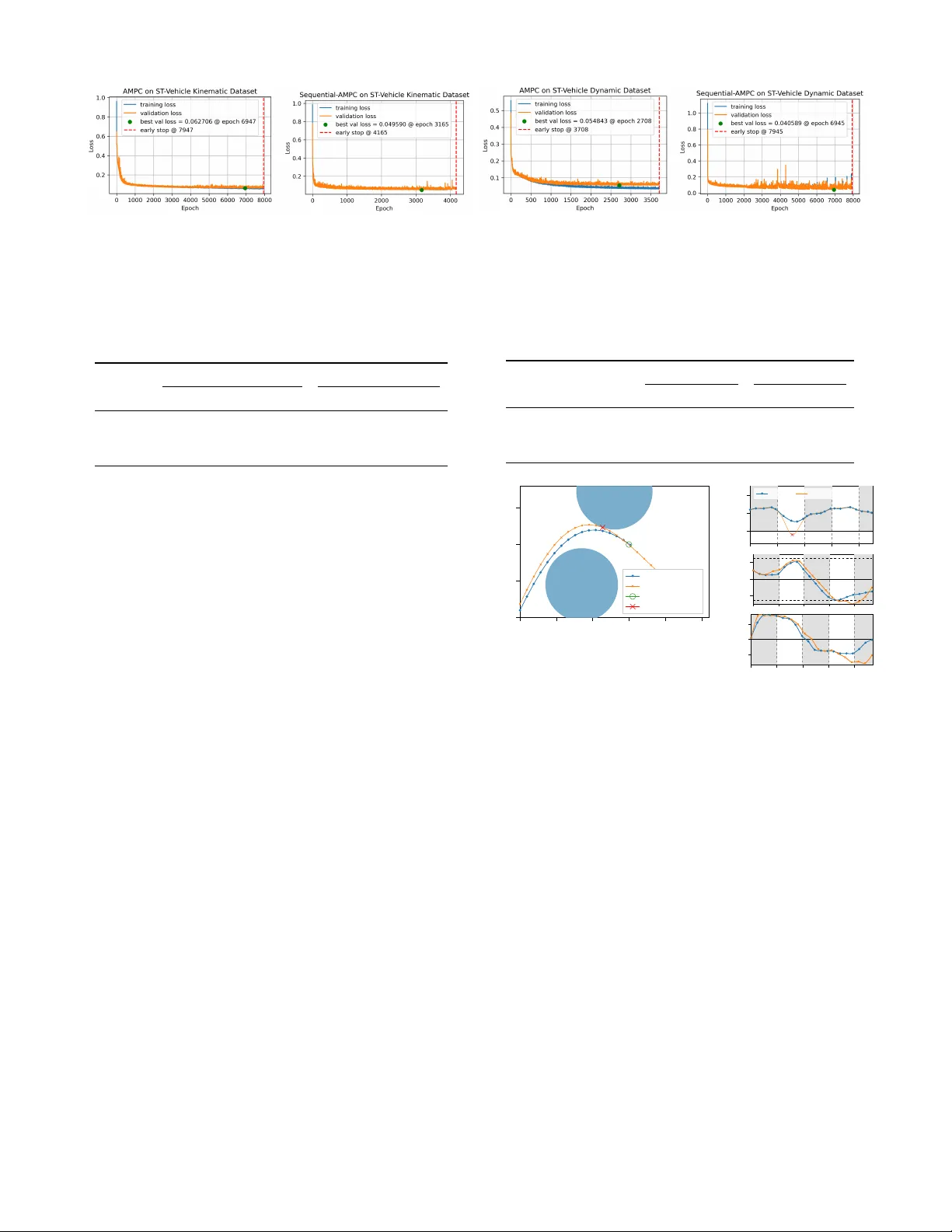
T owards Safe Learning-Based Non-Linear Model Predicti ve Contr ol thr ough Recurrent Neural Network Modeling Mihaela-Larisa Clement 1 , 2 , M ´ onika Farsang 1 , Agnes Poks 3 , Johannes Edelmann 3 , Manfred Pl ¨ ochl 3 , Radu Grosu 1 , Ezio Bartocci 1 Abstract — The practical deployment of nonlinear model pre- dictive contr ol (NMPC) is often limited by online computation: solving a nonlinear program at high contr ol rates can be expensive on embedded hardwar e, especially when models are complex or horizons are long. Learning-based NMPC approximations shift this computation offline b ut typically demand large expert datasets and costly training . W e propose Sequential-AMPC, a sequential neural policy that generates MPC candidate control sequences by sharing parameters across the prediction horizon. For deployment, we wrap the policy in a safety-augmented online evaluation and fallback mechanism, yielding Safe Sequential- AMPC. Compared to a nai ve feedforward policy baseline across several benchmarks, Sequential-AMPC requires substantially fewer expert MPC rollouts and yields candidate sequences with higher feasibility rates and improved closed-loop safety . On high- dimensional systems, it also exhibits better learning dynamics and performance in fewer epochs while maintaining stable validation impro vement where the feedforward baseline can stagnate. I . I N T RO D U C T I O N Modern safety-critical systems (e.g., autonomous vehicles and robots) increasingly rely on NMPC to satisfy strict state and input constraints while optimizing performance. Y et these controllers often must run on embedded or edge hardware with tight latency and compute budgets, motiv ating learning-based MPC methods that accelerate or approximate NMPC while aiming to retain its robustness and safety properties. W ithin this landscape, se veral lines of research have emerged to integrate machine learning on different axes: (i) learning an appr oximation of the MPC policy to avoid online optimization, (ii) learning models used inside MPC to improv e MPC pre- diction quality , and (iii) learning or tuning MPC formulations (costs, constraints, parameters) from data to improve closed- loop performance. A common learning-based NMPC approach is to mimic the MPC feedback policy through supervised learning on offline MPC rollouts: solve MPC for many initial conditions to obtain state–action (or history–action) pairs, then train a function approximator to replace online optimization at runtime [1]–[6]. Most prior work uses feedforward NNs, with recurrent policies explored only in [6]. W e also follow this direction, but we focus on robustness and safety guarantees not addressed in [6]. A complementary line of work learns the predictiv e dy- namics model used within MPC, typically via RNN variants (LSTM/GR U) for system identification, and then embeds the learned model in MPC optimization, often with stability 1 Institute of Computer Engineering, TU W ien, V ienna, Austria 2 AIT Austrian Institute of T echnology , Vienna, Austria 3 Institute of Mechanics and Mechatronics, TU Wien, V ienna, Austria Corr . author: mihaela-larisa.clement@tuwien.ac.at Encoder RNN cell Linear head ... RNN cell RNN cell RNN cell ... ... System Dynamics Safe Online Evaluation Sequential Approximate MPC (Seq-AMPC) Fig. 1. Proposed Sequential Approximate MPC (Seq-AMPC) generates the horizon recursiv ely with a shared simple RNN cell (hidden size 256) and output head, preserving the same final output format ˆ U t ∈ R N × n u . Seq-AMPC replaces Π AMPC of [5], resulting in a better-aligned controller, particularly in producing feasible horizon proposals. For deployment, Seq- AMPC is embedded in a safety-augmented online ev aluation and fallback wrapper: candidate sequences are checked for feasibility and cost, and, if necessary , a safe fallback candidate and terminal controller are applied. W e refer to the overall wrapped controller as Safe Seq-AMPC. or safety v alidation [7]–[9]. In contrast, we assume kno wn dynamics and do not address model learning. Beyond model learning, several works pursue performance- oriented learning of MPC by tuning costs, constraints, or parameters to optimize closed-loop objectives, often while preserving safety via constrained updates [10], [11]. Neural networks also support MPC by warm-starting solvers or via safety filters, b ut warm-starting still requires online optimization with potentially unpredictable runtimes [12]–[14], and safety filters beyond linear systems typically add further online optimization or require uniform approximation error bounds [2], [3], [15]. In contrast, Hose et al. remove online optimization by predicting the full input sequence and applying a fast feasibility/stability check; if the proposal fails, a shifted previous solution plus terminal controller is executed [5]. W e take this approach as our starting point and extend it with a sequential policy architecture. Our work bridges two strands that are typically studied in isolation: safety-certified approximations of MPC policies and sequential (recurrent) policy parameterizations that capture temporal dependence. Building on safe online ev aluation for approximate MPC [5], we replace the feedforward horizon policy with an autoregressiv e RNN that generates the input sequence recursiv ely , as illustrated in Fig. 1. W e call the RNN horizon policy Sequential-AMPC (Seq-AMPC). When deployed inside the safety-augmented ev aluation and fallback mechanism of Algorithm 1, we refer to the ov erall controller as Safe Seq-AMPC. Seq-AMPC consistently outperforms naive AMPC across benchmarks in both open-loop feasibility and closed-loop safety . This suggests that sequential policy structure alone can materially improv e the reliability of safe learning- based MPC, without modifying the safety filter . I I . B A C K G RO U N D In this section, we present the robust NMPC formulation, describe how it can be approximated using safety-augmented neural networks, and provide further details on the architectures and training of feedforward and recurrent neural networks. A. Robust Nonlinear Model Predictive Contr ol W e formulate a robust nonlinear model predictive control (NMPC) scheme for the considered dynamics model. The discrete-time dynamics are giv en by x k +1 = f ( x k , u k ) , where x k ∈ X ⊂ R n x denotes the state and u k ∈ U ⊂ R n u the control input. A rob ust MPC formulation aims to guarantee closed-loop stability and recursiv e constraint satisfaction for all admissible bounded disturbances [16]. T o model actuator uncertainty and model mismatch, we assume that the implemented input is perturbed as u k = ¯ u k + d k with bounded disturbance ∥ d k ∥ ∞ ≤ ε . a) T ube-based feedback parameterization: Instead of directly optimizing over u k , we use an affine pre-stabilizing parameterization u k = K δ x k + v k , where K δ is computed offline by solving a set of linear matrix inequalities (LMIs) to guarantee contraction of the deviation dynamics and robust stability . The feedback term K δ x k guarantees contraction of the de viation dynamics, while v k determines the nominal performance. This decomposition enables robust constraint tightening while preserving the original optimization structure. b) Finite-horizon optimal contr ol pr oblem: Giv en the current state x 0 , we solve at each sampling instant the optimization problem V ⋆ ( x 0 ) = min v 0: N − 1 N − 1 X k =0 ℓ ( x k , K δ x k + v k ) + V f ( x N ) (1) s.t. x k +1 = f ( x k , K δ x k + v k ) , (2) x k ∈ ¯ X , v k ∈ ¯ U , (3) x N ∈ X f . (4) Here, ¯ X and ¯ U denote tightened constraint sets that guarantee robust feasibility of the original constraints X and U . The stage cost is quadratic, ℓ ( x, u ) = ( x − x ref ) ⊤ Q ( x − x ref ) + ( u − u ref ) ⊤ R ( u − u ref ) , with Q ⪰ 0 and R ≻ 0 chosen to balance tracking performance and control ef fort. The terminal cost is giv en by V f ( x ) = x ⊤ P x , where P is obtained from the terminal LMI design and is chosen as an ellipsoid X f = { x | x ⊤ P x ≤ α } with terminal controller u = K f x and P ⪰ 0 . The matrices ( P , K f ) are computed offline to ensure local stability and recursiv e feasibility of the closed-loop system. c) Receding-horizon implementation: At each time step, the optimal sequence v ⋆ 0: N − 1 is computed, and only the first control input u ( t ) = K δ x ( t ) + v ⋆ 0 is applied. The horizon is then shifted forward. This robust NMPC controller serves as the ground-truth policy for dataset generation and defines the feasible input set U N ( x ) used in the approximate MPC scheme described next. B. Appr oximate MPC with Safety-Augmented Neural Networks W e approximate the MPC with a NN policy Π AMPC , which learns to map a state x to an input control sequence u with horizon length N , following the work of Hose et al. [5]. W e augment the NN for safe online ev aluation by checking whether Π AMPC is feasible and selecting between the NN’ s sequence and a safe fallback. This ensures closed-loop safety and con ver gence, as implemented in Algorithm 1. W e call Algorithm 1 instantiated with Π AMPC the Safe AMPC controller . For each state x ( t ) , the NN predicts a sequence ˆ u ( t ) in line 3, which is checked for feasibility . If safe, the lower-cost sequence between ˆ u ( t ) and a fallback ˜ u ( t ) is selected in line 5, and the first input u 0 ( t ) is ex ecuted while updating the safe candidate for the next step in line 9. Algorithm 1: Approximate MPC with safety- augmented NN [5] Require: Approximate mapping Π AMPC : X → U N , Set of feasible input trajectories: U N : X ⇒ U N , x 7→ U N ( x ) ⊆ U N , T erminal feedback controller K f : X f → U , Cost function V : X × U N → R , Safe initial candidate input ˜ u (0) = u init 1 for t ∈ N do 2 x ← x ( t ) // state at time t 3 ˆ u ( t ) ← Π AMPC ( x ) // eval. approx. 4 if ˆ u ( t ) ∈ U N ( x ) then 5 u ( t ) ← arg min u ( t ) ∈{ ˜ u ( t ) , ˆ u ( t ) } V ( x, u ( t )) // choose input with min. cost 6 else 7 u ( t ) ← ˜ u ( t ) // keep candidate seq. 8 u ( t ) ← u 0 ( t ) 9 ˜ u ( t + 1) ← { u ( t ) 1: N − 1 , K f ( ϕ ( N ; x ; u ( t ))) } 10 end C. F eed-forwar d Neural Networks Feed-forward neural networks are parametric function ap- proximators formed by composing multiple nonlinear trans- formations. In the most common setting for tabular or vector inputs, a multi-layer perceptron (MLP) maps an input vector x ∈ R n x to an output ˆ y ∈ R n y through a sequence of affine maps and pointwise nonlinearities, where n x is the input and n y is the output dimension, as follows: z (0) = x, z ( ℓ ) = ϕ  W ( ℓ ) z ( ℓ − 1) + b ( ℓ )  ˆ y = ψ  W ( L +1) z ( L ) + b ( L +1)  . (5) where ℓ = { 1 , . . . , L } , W ( ℓ ) and b ( ℓ ) denote trainable weights and biases, ϕ ( · ) is a hidden-layer activ ation (e.g., ReLU or tanh ), and ψ ( · ) is an output map chosen for the task (e.g., identity for regression). T raining typically minimizes a loss function min θ P i L ( ˆ y i , y i ) of the prediction ˆ y based on all weights denoted by θ and the ground truth value y by gradient- based optimization, with gradients computed efficiently via backpropagation. D. Recurr ent Neural Networks Recurrent neural networks (RNNs) extend this framework to sequential data by introducing a hidden (latent) state h ∈ R n h as a memory component of the network. Gi v en a sequence { x t } N t =1 ∈ R n x , an RNN updates a hidden state { h t } N t =1 ∈ R n h and produces outputs { ˆ y t } N t =1 ∈ R n y according to h t = σ h ( W x x t + W h h t − 1 + b h ) , (6) ˆ y t = σ y ( W y h t + b y ) , (7) with shared parameters across time steps. This weight sharing enables the model to represent temporal dependencies and to condition predictions on past information encoded in h t − 1 . The new hidden state h t at time step t is calculated from the past hidden state h t − 1 and the current input x t . W x ∈ R n h × n x , W h ∈ R n h × n h and b h ∈ R n h are the trainable weights and bias for the hidden state update calculation. W y ∈ R n y × n h and b y ∈ R n y are used for calculating the output prediction ˆ y t ∈ R n y based on the current hidden state h t . T raining RNNs follows the same minimization principle as for feedforward networks, but the loss is typically accumulated ov er the sequence, min θ N X t =1 L ( ˆ y t , y t ) , (8) where θ = { W x , W h , W y , b h , b y } denotes the shared model parameters. Gradients are computed using backpropagation through time (BPTT) [17], which consists of unrolling the recurrent computation over the time horizon N and applying the chain rule through the resulting computational graph. Due to the recurrence in h , the gradient of the loss with respect to a parameter (e.g., W h ) accumulates contributions from all time steps, ∂ L ∂ W h = N X t =1 ∂ L ∂ h t ∂ h t ∂ W h . (9) E. T raining Neural Networks T raining neural networks in v olves optimizing model parame- ters to minimize a task-specific loss function on a giv en dataset. A challenge in this process is prev enting ov erfitting, where the model learns patterns only specific to the training data but fails to generalize to unseen samples. Overfitting is particularly relev ant when using large models or limited datasets. A common strategy to mitigate this ef fect is early stopping, where training is stopped once the validation performance no longer improv es. Dataset size plays a crucial role in determining both generalization performance and model capacity . Larger datasets typically allo w the use of more e xpressi ve models, while smaller datasets require careful control of model complexity to avoid ov erfitting. Consequently , the choice of model size should balance representational power and generalization ability . From a computational perspectiv e, training efficienc y is in- fluenced by both the number of parameters and the architecture of the model. Larger models generally require more memory and longer training times per epoch. Additionally , certain architectures, such as recurrent neural networks, incur higher computational cost per epoch due to sequential processing and BPTT . Therefore, model design must consider not only predictiv e performance but also computational resources and training time constraints. I I I . S E Q U E N T I A L A P P R OX I M A T E M P C D E S I G N W e replace the feedforward predictor with an RNN-based policy to better match NMPC’ s sequential structure and impro ve robustness to distribution shift. W e call this Seq-AMPC which when wrapped by Algorithm 1 yields Safe Seq-AMPC. In purely MLP-based AMPC solutions, the model lacks memory of the learned control from one time step to the next. Due to this, the authors of [5] proposed to learn n y = n c · N sized output, where n c denotes the control dimensionality and N the horizon length. This implies that ˆ y t and ˆ y t + k k ∈ N + are not directly dependent on each other , but are only linked through the one before the final layer of the MLP z ( L ) , on which they both depend. Consequently , the output predictions share a common latent representation but do not interact temporally , i.e., ˆ y t ⊥ ˆ y t + k | z ( L ) . T o overcome this limitation, we propose an RNN-based solution. In this case, the model predicts an output of size n y = n c , and due to its recurrent nature, it can be applied recursiv ely to generate predictions over the horizon of length N , resulting in the same overall output dimensionality as the MLP-based approach. The key difference is the presence of a memory component (hidden state), which preserves temporal dependencies between time steps. In the RNN case, temporal dependencies are captured through the hidden state recursion h t = f θ ( h t − 1 , x t ) , implying that future predictions ˆ y t + k depend recursively on past states and inputs, unlike the conditionally independent outputs produced by the MLP-based approach. While both MLP- and RNN-based architectures are univ ersal function approximators [18], [19], RNNs introduce parameter sharing across time steps and impose a temporal inductiv e bias consistent with dynamical systems. This structural constraint re- duces the effecti v e model complexity and aligns the architecture with the sequential nature of the control problem. Therefore, although no formal guarantee of superior performance exists, theoretical considerations regarding parameter efficiency and in- ductiv e bias motiv ate the in vestigation of RNN-based solutions in this setting. Proposition 1. (Parameter Scaling with Respect to the Horizon Length). Consider (i) an MLP that pr edicts a horizon of length N at once, pr oducing n y = n c · N outputs, and (ii) an RNN that predicts n c outputs per time step with shar ed parameters acr oss time. Assume both models use hidden dimension n h and input dimension n x . Then, for sufficiently lar ge N , the number of trainable parameters of the MLP gr ows linearly in N , wher eas the number of trainable parameters of the RNN is independent of N . Pr oof . Consider an L -layer MLP with hidden width n h and output dimension n y = n c N . The last layer’ s parameter contribution comes from W ( L +1) ∈ R ( n c N ) × n h , b ( L +1) ∈ R ( n c N ) . Hence, the parameter count of this layer is | θ MLP | = n c N n h + n c N = n c N ( n h + 1) , which grows linearly with N . For the RNN, h t = σ h ( W x x t + W h h t − 1 + b h ) , ˆ y t = σ y ( W y h t + b y ) , with W x ∈ R n h × n x , W h ∈ R n h × n h , W y ∈ R n c × n h . The total parameter count is | θ RNN | = n h n x + n 2 h + n c n h + n h + n c , which does not depend on N . Conclusion. For increasing horizon length N , the MLP parameter count grows linearly , | θ MLP | = O ( N ) , whereas the RNN parameter count remains constant, | θ RNN | = O (1) . Hence, for sufficiently large N , the RNN is strictly more parameter- efficient than the horizon-wide MLP . Proposition 2. (Inductive Bias of RNNs for Sequential Control). Consider a discrete-time dynamical system governed by x t +1 = f ( x t , u t ) , wher e x t ∈ R n x is the system state and u t ∈ R n c the contr ol input at time t . Let the objective be to pr edict a sequence of contr ol inputs { u t } N t =1 given the initial state x 0 and possibly intermediate observations. An RNN that updates its hidden state as h t = σ h ( W x x t + W h h t − 1 + b h ) , ˆ u t = σ y ( W y h t + b y ) naturally captur es the temporal dependence of the system, wher eas an MLP pr edicting the entir e horizon at once does not explicitly encode this sequential structure . Claim: The RNN architecture introduces an inductive bias aligned with the system dynamics, which allows it to more ef ficiently represent the class of sequential control policies that obey the Markov property of the system. Pr oof (Ar gument by Structural Alignment). 1) System Dynamics. In a Markovian system, the optimal control at time t depends on the current state x t , which itself is a function of all previous states and controls: x t = f ( t ) ( x 0 , u 0 , . . . , u t − 1 ) . 2) RNN Recurrence. The RNN recursiv ely encodes the history of states and controls in its hidden state h t : h t = g θ ( h t − 1 , x t ) , ˆ u t = g θ ( h t ) , where g θ is the learned transition function. By con- struction, h t contains information about the entire past trajectory , allowing ˆ u t to condition on the relev ant history without explicitly concatenating all previous inputs. 3) MLP Limitation. An MLP predicting the full horizon { ˆ u 1 , . . . , ˆ u T } treats the outputs as conditionally inde- pendent given a shared latent vector z ( L ) . T emporal dependencies must be encoded implicitly in z ( L ) , which may require a larger number of parameters and more data to capture sequential structure. 4) Conclusion. Because the RNN recurrence mirrors the sequential, causal structure of the system dynamics, it imposes an inductiv e bias that aligns with the Markov property . This structural bias reduces the effecti ve hy- pothesis space needed to represent valid control policies, which can lead to more sample-efficient learning and better generalization in sequential tasks. I V . P R O B L E M S E T U P S The selected benchmarks represent high-performance control scenarios with increasing complexity . The quadcopter and single-track vehicle tasks emphasize obstacle avoidance and operate near dynamic and safety limits, making feasibility and constraints management essential. A. Quadcopter Model As a benchmark, we consider the quadcopter model described in [5]. The state vector is defined as x = [ x 1 , x 2 , x 3 , v 1 , v 2 , v 3 , ϕ 1 , ω 1 , ϕ 2 , ω 2 ] ⊤ ∈ R 10 , and the input vector as u = [ u 1 , u 2 , u 3 ] ⊤ ∈ R 3 . The continuous-time dynamics are giv en by ˙ x i = v i , i = 1 , 2 , 3 , (10) ˙ v i = g tan( ϕ i ) , i = 1 , 2 , (11) ˙ v 3 = − g + k T m u 3 , (12) ˙ ϕ i = − d 1 ϕ i + ω i , ˙ ω i = − d 0 ϕ i + n 0 u i , i = 1 , 2 . (13) The steady-state thrust required for hov er is u e, 3 = g m k T . The parameters are chosen as d 0 = 80 , d 1 = 8 , n 0 = 40 , k T = 0 . 91 , m = 1 . 3 , and g = 9 . 81 . Input constraints are | u 1 , 2 | ≤ π 4 and u 3 ∈ [0 , 2 g ] , while the attitude is bounded by | ϕ 1 , 2 | ≤ π 9 . The system is discretized with sampling time T s = 0 . 1 s and prediction horizon N = 10 . W e use quadratic weights Q = diag(20 , 1 , 3 , 1 , 3 , 0 . 01 , 1 , 4 , 1 , 4) and R = diag (8 , 8 , 0 . 8) , placing stronger emphasis on horizontal position and attitude regulation. W e use a dataset of 9.6M feasible initial conditions generated by the NMPC expert. B. Single-T rack V ehicle Models 1) Kinematic Model: W e use a kinematic ground vehicle model for planar navigation with x = [ p x , p y , ψ , v ] ⊤ ∈ R 4 , u = [ δ, a ] ⊤ ∈ R 2 , and Euler forward discretization p x,k +1 = p x,k + T s v k cos ψ k , p y ,k +1 = p y ,k + T s v k sin ψ k , ψ k +1 = ψ k + T s δ, v k +1 = v k + T s a k . W e set T s = 0 . 01 s and horizon N = 40 . Inputs are bounded by a ∈ [ − 6 . 0 , 3 . 2] m/s 2 . and δ ∈ [ − 25 ◦ , 25 ◦ ] , and the speed is constrained by v ∈ [0 , ⟨ v max ⟩ ] . The operating region is restricted to p x , p y ∈ [ ⟨ p min ⟩ , ⟨ p max ⟩ ] . Obstacle av oidance is imposed using the same circular constraints as above, ( p x − o ix ) 2 + ( p y − o iy ) 2 ≥ r 2 safe , i = 1 , . . . , n obs , with obstacle centers sampled within the arena and inactiv e obstacles placed outside. Initial conditions are sampled from p x , p y windows around the start and bounded heading/speed uncertainty , e.g., ψ ∈ [ ψ 0 ± γ ψ ] , v ∈ [ v 0 ± γ v ] . W e use a quadratic tracking cost with Q = diag([10 , 10 , 0 . 2 , 5]) and R = diag ([2 , 4]) . W e generate 55K NMPC-expert demonstra- tions from feasible initial conditions. 2) Dynamic Model: For the dynamic formulation, we employ a single-track model with steering dynamics, x = [ p x , p y , ψ , v , r, β , ˙ v , δ ] ⊤ ∈ R 8 , u = [ ˙ δ , a ] ⊤ ∈ R 2 . The nonlinear dynamics capture yaw-rate coupling, lateral tire forces, and actuator lag, and are discretized with sampling time T s = 0 . 01 and prediction horizon N = 40 . W e use vehicle geometry ℓ f = 1 . 35 m, ℓ r = 1 . 21 m. This model explicitly represents lateral velocity via the side-slip angle β and yaw-rate r , allo wing the controller to re gulate stability-rele v ant quantities. Control inputs are constrained by ˙ δ ∈ [ − 1 . 0 , 1 . 0] rad/s and a ∈ [ − 6 . 0 , 3 . 2] m/s 2 . The steering angle is bounded by δ ∈ [ − 25 ◦ , 25 ◦ ] . The operating region is restricted to p x , p y ∈ [ ⟨ p min ⟩ , ⟨ p max ⟩ ] and v ∈ [0 , ⟨ v max ⟩ ] . Obstacle a voidance is enforced by n obs circular obstacles with centers o i = ( o ix , o iy ) and safety radius r safe , ( p x − o ix ) 2 + ( p y − o iy ) 2 ≥ r 2 safe , i = 1 , . . . , n obs , imposed at every stage. Initial conditions are sampled from a bounded set around the start state, e.g., p x , p y ∈ [ p x, 0 ± γ p ] , ψ ∈ [ ψ 0 ± γ ψ ] , v ∈ [ v 0 ± γ v ] , with remaining states initialized consistently . The quadratic state and input cost terms T ABLE I O P EN - L O OP C OM PA RI S O N O F N AI V E A M P C ( M L P ) A N D N AI V E S E Q - A M P C ( R N N ) U S I N G 1 ,0 0 0 U N I F OR M L Y S A M P LE D P O I N TS F RO M A D I SJ O I N T T ES T DA TAS E T . Epochs D E N OT E T H E N UM B E R O F E P O CH S UN T I L E A RLY S T OP P I NG ( P A T I EN C E = 1 , 00 0 ) O R T E R M IN A T IO N AMPC Seq-AMPC Epochs Feas. Epochs Feas. T ask [ 10 3 ] [%] [ 10 3 ] [%] Quadcopter 100 72 2.75 83.6 ST -V ehicle Kinematic 7 . 9 35.3 4.1 36.4 ST -V ehicle Dynamic 3.7 35.6 7 . 9 39.5 T ABLE II C L OS E D - LO O P C O M P A RI S O N O F S A F E A M PC ( ML P ) A N D S A F E S E Q - A M P C ( R N N ) F RO M 1, 0 0 0 R A N DO M FE A S I BL E I N I T IA L STA T E S . W E R E PO RT TH E PE R C E NTAG E O F S A F E RO L L O UT S ( S A F E ) G IV E N B Y TH E NA I V E N N A N D T H E P E RC E N T AG E O F RO LL O U T S W H ER E T H E S A F E C A ND I DATE W A S AP P L I ED ( I N T E RV . ) . AMPC Seq-AMPC T ask Safe [%] Interv . [%] Safe [%] Interv . [%] Quadcopter 84.8 8.2 89.1 78.8 ST -V ehicle Kinematic 92.2 90.6 92.9 90.0 ST -V ehicle Dynamic 54.1 94.4 58.7 95.6 hav e weights Q = diag([10 , 10 , 0 . 5 , 0 . 5 , 0 . 2 , 5 , 1 , 5]) and R = diag([2 , 4]) and a terminal cost V f ( x ) = x ⊤ P x with terminal ingredients computed offline. The size of the expert dataset is 116K. V . R E S U LT S Across benchmarks, we compare the AMPC policy (MLP layers with 1 million trainable parameters) [5] to the proposed Sequential-AMPC (RNN with only 0.5 million parameters) under the same safety-augmented wrapper (Alg. 1). W e report (i) open-loop feasibility of the predicted sequence with respect to the feasible set U N ( x ) (T able I), and (ii) closed-loop safety under the wrapper measured by the fraction of safe rollouts and the fraction of rollouts in which the safe candidate is applied (T able II and T able III). As an open-loop statistical ev aluation, T able I reports feasibility when initialized from the successor state reached by applying the naiv e controller’ s predicted control action at the initial feasible test state. The test set is disjoint from training. In the closed-loop experiments, we define the safety per- centage as the proportion of test rollouts whose closed-loop trajectories satisfy the state and input constraints at all time steps (and, where applicable, the terminal constraint). Each rollout is initialized from the post-action state obtained by applying the dataset’ s safe initial candidate. A. Quadcopter On the quadcopter task, naiv e Sequential-AMPC attains substantially higher feasibility than AMPC while requiring Fig. 2. Learning curves of AMPC (MLP) and Seq-AMPC (RNN) on the single-track vehicle model tasks, for the kinematic model on the left and the dynamic model on the right. Seq-AMPCs con verged to lower v alidation losses. Early stopping was used to avoid overfitting to the training datasets. T ABLE III Q UA D CO P T ER S EQ - A M PC ( R NN ) S C A L IN G WI T H D E C R EA S I N G T RA I N I NG S A MP L E S I Z ES . W E R EP O RT T R A I NI N G C O M PU T E ( E P O CH S ) , O P E N - L O O P F E AS I B I LI T Y R A T E ( F EA S . ) , A N D C L O SE D - L OO P ME T R I CS ( S A F E , I N TE RV . ) . T raining Closed-loop Samples Epochs [ 10 3 ] Feas. [%] Safe [%] Interv . [%] 1x 2.75 83.6 89.1 78.8 1/4x 4 . 92 83.5 87.5 78.4 1/10x 6 . 59 79.9 82.8 78.2 ≈ 97% fewer training epochs (T able I). In closed loop, it also improv es safety to 89 . 1% safe rollouts (T able II). T o test whether recurrence can reduce data requirements by lev eraging memory , we trained with smaller datasets. Even at 1 / 10 × data, Seq-AMPC achiev es 82 . 8% closed-loop safety (T able III), remaining close to the AMPC baseline at full data ( 84 . 8% , T able II). B. Single-T rack V ehicle Models For the vehicle benchmarks with obstacles, Fig. 2 presents the training curves for AMPC and Seq-AMPC, where the Seq- AMPC demonstrates better learning capabilities, achieving lower validation loss on both benchmarks. T able I shows that Seq-AMPC improves feasibility over AMPC, with mixed training-epoch requirements depending on task. Importantly , the lower AMPC epoch count on the dynamic benchmark reflects early stopping triggered by stagnating/diver ging v alidation loss (Fig. 2), not faster conv ergence; Seq-AMPC trains longer because its validation loss continues to improve. For the kinematic v ehicle benchmark with obstacles, with half the amount of training epochs, the Seq-AMPC (RNN) yields a modest feasibility improv ement ( 36 . 4% vs. 35 . 3% ) For the dynamic bicycle model with obstacles, the Seq-AMPC (RNN) improves feasibility to 39 . 5% compared to 35 . 6% , albeit requiring longer training since validation loss continues improving. Fig. 3 shows the closed-loop performance of a naiv e NN versus a safety NN in a vehicle obstacle-av oidance task. Both controllers start from the same initial state and aim to reach a target while av oiding circular obstacles. The naiv e (in orange) initially navig ates well but ev entually collides with an obstacle (marked by a red cross). In contrast, the safety NN (in blue) maintains a safe distance from obstacles and successfully reaches the target without violations. T ABLE IV R E AS O N S F O R A P PLY IN G TH E SA F E C A N D ID A T E O N TH E VE H I C LE B E NC H M A RK S ( M U L T I PL E RE A S O NS M A Y A PP LY ). P ER C E N T AG E S A RE C O MP U T E D OV E R RO L L OU T S W H E RE T HE S AF E CA N D I DA T E I S A P PL I E D . AMPC Seq-AMPC T ask State T erm. Cost State T erm. Cost Quadcopter 72.5 2.6 40.6 9.2 98.5 44.5 ST -V ehicle Kinematic 0.0 90.5 57.7 0.0 89.5 64.0 ST -V ehicle Dynamic 0.0 90.0 79.6 0.0 90.0 71.6 0 1 2 3 4 5 0 1 2 3 x 2 x 1 Safe Trajectory Naive Trajectory T arget Collision 0 0 . 1 0 . 2 crash dist. collision [m] Safe NN Naive NN − 20 0 20 δ [rdeg] 0 1 2 3 4 − 2 0 2 time [s] a cmd [m/s 2 ] Fig. 3. Examples of a nai ve and a safe trajectory are shown. T wo blue-colored blocks are the obstacles that the vehicle needs to avoid. The non-safe trajectory collides at the red cross while the safe trajectory is able to reach and stop at the target point without collision. In the right side of Fig. 3, the closed-loop signals show that the nai ve controller’ s distance to collision falls belo w zero, indicating a crash, while the safety-augmented controller remains viable. This highlights how naive execution can lead to unsafe behavior , while the safety mechanism pre vents violations by rejecting unsafe NN proposals. Such safety features are critical in vehicle control, where small steering and acceleration errors can accumulate, leading to significant deviations. The safety NN controller continuously enforces constraints to ensure reliable trajectory tracking and safe maneuver execution in dynamic scenarios. In closed loop (T able II), Seq-AMPC consistently improv es the fraction of safe rollouts on both vehicle benchmarks. For the kinematic model, safety increases from 92 . 2% to 92 . 9% while slightly reducing interventions ( 90 . 6% → 90 . 0% ), indicating that the learned sequential policy is marginally more reliable under the safety wrapper . For the dynamic model, Seq-AMPC yields a larger safety gain ( 54 . 1% → 58 . 7% ) but interventions remain near-saturated for both methods ( ≈ 95% ), suggesting that the safety wrapper is frequently falling back to the shifted candidate. T able IV breaks down, over time steps where the safe candidate is applied, which acceptance checks the NN proposal fails: State (predicted state/input feasibility along the rollout), T erm. (terminal-set membership of X N ), and Cost (does not reduce total MPC cost relati ve to the shifted-and-appended stored candidate). On the quadcopter, AMPC interventions are mainly feasibility-driv en ( State 72 . 5% , T erm. 2 . 6% ), while Seq- AMPC largely remov es feasibility violations ( State 9 . 2% ) but is rejected mostly for terminal-set failures ( T erm. 98 . 5% ), with both often failing the cost gate ( Cost 40 - 45% ). On both vehicle benchmarks, State is 0 . 0% for AMPC and Seq-AMPC, so interventions are not caused by predicted constraint (including obstacle) violations but by T erm. and Cost : proposals are typically feasible yet frequently neither reach the terminal region within the horizon nor improve on the conservati ve shifted candidate. V I . S U M M A RY A N D C O N C L U S I O N S The proposed Safe Seq-AMPC is a safe learning-based approximation of robust NMPC that shifts online optimization to of fline training while preserving safety and con vergence through a safety-augmented ev aluation wrapper . W e introduce Seq-AMPC to replace horizon-wide feedforward prediction using a sequential RNN policy that generates the control horizon recursively with shared parameters. This introduces a temporal bias aligned with the structure of NMPC solutions and av oids parameter growth with the horizon length, a significant issue with feedforward AMPC. Across all benchmarks, Seq-AMPC impro ves ov er the feedforward AMPC baseline under the safety-augmented deployment: it achieves higher open-loop feasibility and higher closed-loop safety rates, while exhibiting more stable learning dynamics (continued validation improvement rather than early stagnation on the harder vehicle models). Moreover , on the quadcopter data, Seq-AMPC attains higher feasibility and safety with substantially fewer training epochs, and remains effecti v e under significant reductions in training data. At the same time, the closed-loop statistics show that interventions can remain high, particularly on the obstacle- av oidance vehicle tasks (and near-saturated on the dynamic model), meaning the wrapper still frequently relies on the shifted candidate plus terminal controller . T ogether with the intervention-reason breakdown, this suggests that the main bottleneck is producing proposals that satisfy the wrapper’ s acceptance tests, especially on terminal-set attainment. Future work will therefore focus on reducing terminal-set failures and improving cost improvement rates (e.g., terminal-aware objecti ves, curriculum sampling near X f , and losses that better align with the MPC value), with the goal of maintaining safety while reducing fallback frequency which is computationally more expensiv e. R E F E R E N C E S [1] M. Hertneck, J. K ¨ ohler , S. Trimpe, and F . Allg ¨ ower , “Learning an approximate model predictiv e controller with guarantees, ” IEEE Contr ol Systems Letters , vol. 2, no. 3, pp. 543–548, 2018. [2] B. Karg and S. Lucia, “Efficient representation and approximation of model predictive control laws via deep learning, ” IEEE transactions on cybernetics , vol. 50, no. 9, pp. 3866–3878, 2020. [3] J. A. Paulson and A. Mesbah, “ Approximate closed-loop robust model predictiv e control with guaranteed stability and constraint satisfaction, ” IEEE Control Systems Letters , vol. 4, no. 3, pp. 719–724, 2020. [4] H. Alsmeier, L. Theiner , A. Savchenko, A. Mesbah, and R. Findeisen, “Imitation learning of mpc with neural networks: Error guarantees and sparsification, ” in 2024 IEEE 63r d Conference on Decision and Control (CDC) . IEEE, 2024, pp. 4777–4782. [5] H. Hose, J. K ¨ ohler , M. N. Zeilinger, and S. Trimpe, “ Approximate non-linear model predictive control with safety-augmented neural networks, ” IEEE Tr ansactions on Control Systems T echnolo gy , vol. 33, no. 6, pp. 2490–2497, Nov . 2025, arXi v:2304.09575 [eess]. [Online]. A vailable: http://arxiv .org/abs/2304.09575 [6] Z. Liu, J. Duan, W . W ang, S. E. Li, Y . Y in, Z. Lin, and B. Cheng, “Recurrent model predictive control: Learning an explicit recurrent controller for nonlinear systems, ” IEEE T ransactions on Industrial Electr onics , vol. 69, no. 10, pp. 10 437–10 446, 2022. [7] F . Bonassi, M. Farina, J. Xie, and R. Scattolini, “On Recurrent Neural Networks for learning-based control: Recent results and ideas for future dev elopments, ” Journal of Process Contr ol , vol. 114, pp. 92–104, Jun. 2022. [Online]. A vailable: https://linkinghub.else vier .com/retrie ve/pii/ S0959152422000610 [8] E. T erzi, F . Bonassi, M. Farina, and R. Scattolini, “Model predictiv e control design for dynamical systems learned by Long Short-T erm Memory Networks, ” Aug. 2020, arXiv:1910.04024 [eess]. [Online]. A vailable: http://arxiv .org/abs/1910.04024 [9] K. Huang, K. W ei, F . Li, C. Y ang, and W . Gui, “LSTM-MPC: A Deep Learning Based Predictive Control Method for Multimode Process Control, ” IEEE T ransactions on Industrial Electr onics , vol. 70, no. 11, pp. 11 544–11 554, Nov . 2023. [Online]. A v ailable: https://ieeexplore.ieee.or g/document/9994755/ [10] S. Gros and M. Zanon, “Learning for MPC with stability & safety guarantees, ” Automatica , vol. 146, p. 110598, Dec. 2022. [Online]. A vailable: https://linkinghub.else vier .com/retrie ve/pii/ S0005109822004605 [11] S. Sawant, A. S. Anand, D. Reinhardt, and S. Gros, “Learning-based MPC from Big Data Using Reinforcement Learning, ” Jan. 2023, arXiv:2301.01667 [eess]. [Online]. A vailable: http://arxiv .org/abs/2301. 01667 [12] M. Klau ˇ co, M. Kal ´ uz, and M. Kvasnica, “Machine learning-based warm starting of activ e set methods in embedded model predictive control, ” Engineering Applications of Artificial Intellig ence , vol. 77, pp. 1–8, 2019. [13] S. W . Chen, T . W ang, N. Atanasov , V . Kumar , and M. Morari, “Large scale model predictive control with neural networks and primal active sets, ” Automatica , vol. 135, p. 109947, 2022. [14] Y . V aupel, N. C. Hamacher, A. Caspari, A. Mhamdi, I. G. Ke vrekidis, and A. Mitsos, “ Accelerating nonlinear model predictive control through machine learning, ” Journal of pr ocess contr ol , vol. 92, pp. 261–270, 2020. [15] A. Didier, R. C. Jacobs, J. Sieber, K. P . W abersich, and M. N. Zeilinger , “ Approximate Predictive Control Barrier Functions using Neural Networks: A Computationally Cheap and Permissi ve Safety Filter, ” Jul. 2023, arXiv:2211.15104 [eess]. [Online]. A v ailable: http://arxiv .org/abs/2211.15104 [16] J. Rawlings, D. Mayne, and M. Diehl, Model Pr edictive Contr ol: Theory, Computation, and Design . Nob Hill Publishing, 2017. [Online]. A vailable: https://books.google.at/books?id=MrJctAEA CAAJ [17] P . J. W erbos, “Backpropagation through time: what it does and how to do it, ” Pr oceedings of the IEEE , vol. 78, no. 10, pp. 1550–1560, 2002. [18] K. Hornik, M. Stinchcombe, and H. White, “Multilayer feedforward networks are universal approximators, ” Neural networks , vol. 2, no. 5, pp. 359–366, 1989. [19] A. M. Sch ¨ afer and H. G. Zimmermann, “Recurrent neural networks are univ ersal approximators, ” in International conference on artificial neural networks . Springer, 2006, pp. 632–640.