Reflected diffusion models adapt to low-dimensional data

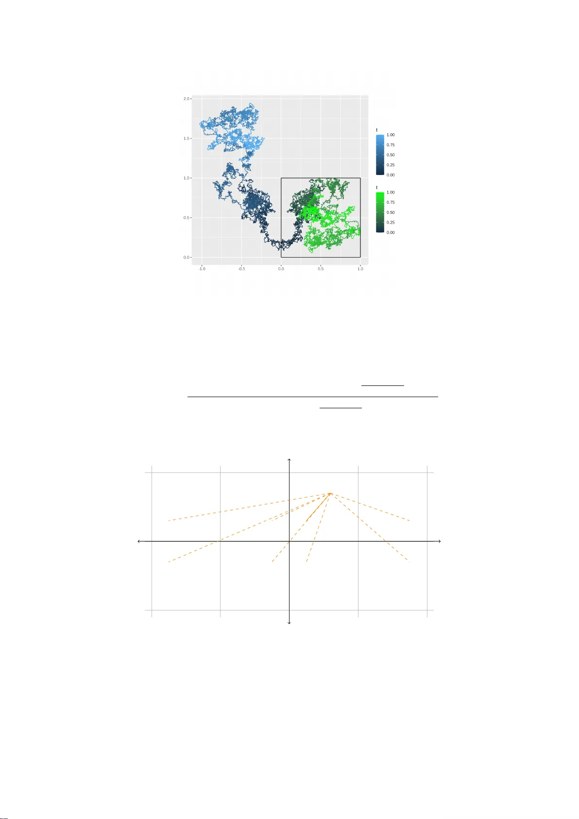
Reected diusion models adapt to low-dimensional data Asbjørn Holk ∗ Claudia Strauch † Lukas Tr ottner ‡ March 26, 2026 While the mathematical foundations of score-based generative models are increasingly well understood for unconstrained Euclidean spaces, many practical applications involve data restricted to bounded domains. This pap er provides a statistical analysis of reected diusion models on the hypercube [0 , 1] 𝐷 for target distributions supported on 𝑑 -dimen- sional linear subspaces. A primary challenge in this setting is the absence of Gaussian transition kernels, which play a central role in standard theory in ℝ 𝐷 . By employing an easily implementable innite series expansion of the transition densities, we develop an- alytic tools to b ound the score function and its approximation by sparse ReLU networks. For target densities with Sob olev smoothness 𝛼 , we establish a convergence rate in the 1 - W asserstein distance of order 𝑛 − 𝛼 +1− 𝛿 2 𝛼 + 𝑑 for arbitrarily small 𝛿 > 0 , demonstrating that the generative algorithm fully adapts to the intrinsic dimension 𝑑 . These results conrm that the presence of reecting boundaries does not degrade the fundamental statistical eciency of the diusion paradigm, matching the almost optimal rates known for uncon- strained settings. 1. Introduction Deep generative models constitute a broad and rapidly evolving class of methods for learning complex data distributions from samples, with score-based diusion models [ 27 ] emerging as a particularly powerful dynamic paradigm in recent years. Motivated by the fact that many modern data sets are intrinsically low-dimensional yet embedde d in high-dimensional b ounded ambient spaces, we study the statistical performance diusion-base d generative modelling for probability measures supporte d on lower-dimensional manifolds within a bounded domain. The study of the statistical performance of diusion models has become a central avenue of research in statistics for machine learning. Several papers [ 1 , 5 , 6 , 8 , 9 , 16 , 23 , 26 , 32 , 37 ] consider the con- vergence of such algorithms in the standard setting of an Ornstein–Uhlenb eck (OU in the following) noising model under dierent regularity and structural assumptions on the target distribution as well as dierent score approximation classes such as neural networks with or without sparsity assumptions and kernel-type estimators. W e provide more details on existing r esults for unconstrained models and how they relate to our work in the discussion in Section 4 , but for now fo cus on the class of reected diusion models that we consider here. Such generative models were rst introduced in [ 11 , 20 ] motivated by the fact that practical imple- mentations of the generative backward process often rely on thresholding proce dures to enforce geo- metric constraints on the data, even though the for ward OU training model ignores such constraints. T o overcome such theoretical discrepancies [ 11 , 20 ] suggest to use a reected diusion process as driver ∗ Aarhus University , Department of Mathematics, Ny Munkegade 118, 8000 Aarhus C, Denmark. Email: a.holk@math.au.dk † Heidelberg University , Institute for Mathematics, Im Neuenheimer Feld 205, 69120 Heidelberg, Germany . Email: strauch@math.uni-heidelberg.de ‡ University of Stuttgart, Department of Mathematics, W ankelstraße 5, 70563 Stuttgart, Germany . Email: lukas.trottner@isa.uni-stuttgart.de 1 of noise instead. This allows to follow the same time-reversal rationale underlying unconstraine d dif- fusion models since the time-r eversal of a reected diusion is again a r eected diusion with adjusted drift incorporating the information on the target data provided by the time evolution of the score , that is the log-gradient of the forward marginals given initialisation in the data distribution. First statistical guarantees for such mo dels were given in [ 13 ] under the assumption that the data distribution has full support on the bounde d reection domain with Sobolev density bounded away from zero. The goal of this paper is to extend this analysis to singular target distributions supported on a lower-dimensional manifold 𝑀 ⊂ [0 , 1] 𝐷 and to demonstrate that the convergence rate of reecte d diusion models adapt to the intrinsic dimension of the data. In doing so, w e pro vide the rst rigorous statistical analysis of diusion-based constrained generative models on b ounded domains that explic- itly accounts for low-dimensional data structures. This is particularly imp ortant from both an applied and a theoretical perspective in light of the so-called manifold hypothesis [ 10 , 18 , 21 ]. It postulates that image or text data ( and many others) although being extremely high-dimensional have common struc- tural features that make them supporte d on (unions of ) much lower dimensional manifolds. Empirical evidence of this has, e .g., been provided by [ 2 , 25 , 28 ], which makes the manifold hypothesis a r eason- able explanation for the tremendous success of de ep generative models, provided that their adaptivity to intrinsic lower-dimensional geometric structures can be theoretically veried. As a natural starting point, we focus on the simplied case where 𝑀 lies in a linear subspace of ℝ 𝐷 . This agrees with the route taken by rst studies on adaptivity of unconstrained diusion models to lower-dimensional data [ 6 , 23 ] and provides an important foundation for further investigations into more complex manifold structur es. Our main contributions can be summarised as follows: • While existing literature on manifold adaptation relies fundamentally on the Gaussian transition kernels of unconstrained OU processes, we develop analytic to ols to control the score function associated with reected Brownian motion on the hypercube . Compared to [ 13 ] we do not work with an eigenfunction expansion of the the score, but use the simple geometry of the hypercube together with symmetries of reected Brownian motion to expand the transition densities as an innite mixture of restricted Gaussian densities. This allows us to provide precise b ounds on the spatial growth of the score and its singular b ehaviour as 𝑡 ↘ 0 , ee ctively decoupling the b oundary eects of the domain from the concentration of the measure 𝜇 around the low- dimensional subspace 𝑀 . • W e prove that, despite the analytic complexities intr oduced by the r eecting boundaries and the resulting non-Gaussian transition densities, denoising score matching via sparse ReLU networks achieves the required approximation rates. In particular , we demonstrate that the complexity of the estimator dep ends only on the intrinsic dimension 𝑑 of the linear subspace supporting the data, rather than the ambient dimension 𝐷 . • W e derive an upper bound for the 1 - W asserstein distance b etween the target distribution and the law of the generated samples. The established rate of 𝑂 ( 𝑛 −( 𝛼 +1− 𝛿 )/(2 𝛼 + 𝑑 ) ) conrms that imposing hard physical constraints via reection on [0 , 1] 𝐷 does not degrade the fundamental statistical eciency of the diusion model, matching the almost optimal rates known for unconstrained dynamics. In the following, we summarise the generative and statistical estimation procedure, introduce and discuss our assumptions on the target distribution and provide an informal version of our main result on 1- W asserstein convergence rates of reected diusion models. Forward reected diusion Let 𝜇 be a target probability distribution on ℝ 𝐷 , concentrated on a com- pact 𝑑 -dimensional manifold 𝑀 ⊂ [0 , 1] 𝐷 , where possibly 𝑑 ≪ 𝐷 . Given an i.i.d. sample of data with distribution 𝜇 , our aim is to generate approximate samples for 𝜇 in a two-step proce dure via a time- rev ersal mechanism for reected diusions. 2 As a rst step, we perturb 𝜇 by adding isotropic noise through a reected Brownian motion on the hypercube. Sp ecically , we consider the reected SDE d 𝑋 𝑡 = d 𝐵 𝑡 + 𝑛 ( 𝑋 𝑡 ) d 𝐿 𝑡 , 𝑋 0 ∼ 𝜇 , (1.1) where ( 𝐵 𝑡 ) 𝑡 ≥ 0 is a standard 𝐷 -dimensional Brownian motion, 𝑛 ( 𝑥 ) denotes an inward-pointing nor- mal vector at 𝑥 ∈ 𝜕 [0 , 1] 𝐷 , and ( 𝐿 𝑡 ) 𝑡 ≥ 0 is the local time of ( 𝑋 𝑡 ) 𝑡 ≥ 0 at 𝜕 [0 , 1] 𝐷 , i.e., a one-dimensional, continuous and non-decreasing process satisfying 𝐿 𝑡 = ∫ 𝑡 0 𝟏 { 𝑋 𝑠 ∈ 𝜕 [0 , 1] 𝐷 } d 𝐿 𝑠 and ∫ 𝑡 0 | 𝑛 ( 𝑋 𝑠 ) | d 𝐿 𝑠 < ∞ almost surely . The presence of the stochastic forcing term 𝑛 ( 𝑋 𝑡 ) d 𝐿 𝑡 in the dynamics prevents the process from escaping the unit cube by normally reecting it back into the interior when it hits the boundar y . Note that for b oundary points 𝑥 ∈ 𝜕 [0 , 1] 𝑑 where two or more faces of the cube intersect, the direction of 𝑛 ( 𝑥 ) is not uniquely dene d. If for 𝑥 ∈ 𝜕 [0 , 1] 𝐷 , we let 𝐼 ( 𝑥 ) , 𝐽 ( 𝑥 ) ⊂ [ 𝐷 ] denote the indices of 𝑥 for which 𝑥 𝑖 = 0 and 𝑥 𝑗 = 1 , respectively , we spe cify 𝑛 ( 𝑥 ) = ∑ 𝑖 ∈ 𝐼 ( 𝑥 ) 𝑒 𝑖 − ∑ 𝑗 ∈ 𝐽 ( 𝑥 ) 𝑒 𝑗 , where 𝑒 𝑖 is the 𝑖 -th standard unit vector in ℝ 𝐷 . In particular , 𝑛 ( 𝑥 ) is the unique inward p ointing normal vector on smooth parts of the cub e boundar y , where faces do not intersect. The particular choice on the non-smooth part of the boundar y 𝐸 ≔ { 𝑥 ∣ | 𝐼 ( 𝑥 ) | + | 𝐽 ( 𝑥 ) | > 1} is without consequences, since the reected Brownian motion will never hit 𝐸 almost surely when started in [0 , 1] 𝐷 ⧵ 𝐸 , cf. [ 36 , Theorem 1.1] and we will assume without further mention that supp( 𝜇 ) ∩ 𝐸 = ∅ . Existence and pathwise uniqueness of strong solutions for general reected diusions in b ounded convex domains has b een shown in [ 31 ] under mild conditions on the co ecients, which are satised for the Brownian case considered here . In particular , be cause of the simple geometry of [0 , 1] 𝐷 and the normal reection direction, the 𝑖 -th coordinate 𝑋 𝑖 of the strong solution of ( 1.1 ) is a strong solution to the one-dimensional reected SDE d 𝑋 𝑖 𝑡 = d 𝐵 𝑖 𝑡 − sgn( 𝑋 𝑖 𝑡 ) d 𝐿 𝑖 𝑡 , where 𝐿 𝑖 is the lo cal time at {0 , 1} and sgn( 𝑥 ) = −1 for 𝑥 ≤ 0 and sgn( 𝑥 ) = 1 for 𝑥 > 0 . Thus, conditional on the initialisation 𝑋 0 , the components of 𝑋 are independent r eected Brownian motions on [0 , 1] and 𝐿 = ∑ 𝐷 𝑖 =1 𝐿 𝑖 almost surely . The boundar y local times 𝐿 𝑖 at the faces ar e characterised via the occupation limit 𝐿 𝑖 𝑡 = lim 𝜀 ↓ 0 1 2 𝜀  𝑡 0 𝟏 [0 ,𝜀 ]∪[1− 𝜀 , 1] ( 𝑋 𝑖 𝑠 ) d 𝑠 , which hold both almost surely and in 𝐿 2 , uniformly on relatively compact sets in 𝑡 , se e [ 3 , The orem 2.6] in a more general context. Consequently , 𝐿 𝑡 = lim 𝜀 ↓ 0 1 2 𝜀  𝑡 0 𝐷  𝑖 =1 𝟏 [0 ,𝜀 ]∪[1− 𝜀 , 1] ( 𝑋 𝑖 𝑠 ) d 𝑠 , (1.2) uniformly in 𝐿 2 and almost sur ely on relativ ely compact sets of 𝑡 . In the follo wing, w e let 𝑝 𝑡 denote the density of 𝑋 𝑡 wrt Lebesgue measure on ℝ 𝐷 . Time reversal and generative sampling Fix a terminal time 𝑇 > 0 , and dene the time-reversed process  𝑋 𝑡 ≔ 𝑋 𝑇 − 𝑡 for 𝑡 ∈ [0 , 𝑇 ] . Then, there exists a Brownian motion ( 𝐵 𝑡 ) 𝑡 ≥ 0 such that  𝑋 satises the reected SDE d  𝑋 𝑡 = ∇ log 𝑝 𝑇 − 𝑡 (  𝑋 𝑡 ) d 𝑡 + d 𝐵 𝑡 + 𝑛 (  𝑋 𝑡 ) d 𝐿 𝑡 ,  𝑋 0 ∼ 𝑝 𝑇 , (1.3) where 𝐿 𝑡 ≔ 𝐿 𝑇 − 𝐿 𝑇 − 𝑡 is the local time of  𝑋 at the boundar y 𝜕 [0 , 1] 𝐷 . This result is proved in [ 4 , Theorem 2.5] for more general reected diusions on smooth domains, while [ 11 , Theorem 3.2] give an instructive probabilistic pr oof inspir ed by the non-reected case [ 12 ] for r eected Bro wnian motion on precompact, smo oth convex domains. Their proof relies on the b oundary o ccupation limit charac- terisation of the local time, which in our case is pr ovided by ( 1.2 ), and sucient smoothness properties of the transition densities of 𝑋 𝑡 , which in our model can be veried base d on the representation given 3 in Lemma 2.2 . Thus, even though the unit cube [0 , 1] 𝐷 is non-smooth, its simple geometry allo ws us to provide the technical tools needed to follow the proof of [ 11 , Theorem 2.3] to verify ( 1.3 ). If the score function 𝑠 0 ( 𝑥 , 𝑡 ) ≔ ∇ log 𝑝 𝑡 ( 𝑥 ) were known, then simulating ( 1.3 ) would yield exact samples from 𝜇 at time 𝑇 . Since 𝑝 𝑡 and 𝑠 0 depend on the unknown target distribution, they must be approximated from data. Approximate backward diusion. Given an approximation 𝑠 ( 𝑥 , 𝑡 ) of the score function, we instead consider the reected SDE d 𝑋 𝑠 𝑡 = 𝑠 ( 𝑋 𝑠 𝑡 , 𝑇 − 𝑡 ) d 𝑡 + d 𝐵 𝑡 + 𝑛 ( 𝑋 𝑠 𝑡 ) d 𝐿 𝑡 , 𝑋 𝑠 0 ∼ U ([0 , 1] 𝐷 ) . (1.4) Several structural features of the proposed framework motivate the use of reecte d diusions on the hypercube. First, the state space [0 , 1] 𝐷 is natural in many applications, including image and signal generation, and reection provides a principle d mechanism to ensure that generated samples remain within prescribed bounds. Second, the forward process ( 1.1 ) has zero drift and unit diusion, which allows for an explicit representation of its transition kernel (see Lemma 2.1 ) and substantially simpli- es the probabilistic analysis. Third, the uniform distribution on [0 , 1] 𝐷 is invariant for the for ward reected Brownian motion, yielding a simple and practically convenient initialisation for the backward dynamics. For numerical stability , we do not run the backward dynamics all the way to time 𝑇 , but instead output the sample 𝑋 𝑠 𝑇 − 𝑇 for some small 𝑇 > 0 . This introduces three distinct sources of error: (i) the truncation error due to early stopping at time 𝑇 ; (ii) the initialisation error fr om starting at stationarity rather than 𝑝 𝑇 ; (iii) the appro ximation error from using 𝑠 instead of the true score 𝑠 0 . Error metric. Our goal is to quantify the discrepancy b etween 𝜇 and the law of the generated samples. Since the algorithm produces a random probability measure as the terminal law of a stochastic pr ocess, a natural notion of error is provided by W asserstein distances. More specically , our error criterion is the 1 - W asserstein distance, for probability measur es 𝜈 1 , 𝜈 2 on [0 , 1] 𝐷 dened by W 1 ( 𝜈 1 , 𝜈 2 ) ≔ inf 𝜋 ∈Π( 𝜈 1 ,𝜈 2 )  [0 , 1] 𝐷 ×[0 , 1] 𝐷 | 𝑥 − 𝑦 | 𝜋 (d 𝑥 , d 𝑦 ) , where Π( 𝜈 1 , 𝜈 2 ) denotes the set of all couplings of 𝜈 1 and 𝜈 2 . Unlike divergences based on densities, W 1 remains meaningful when 𝜈 1 or 𝜈 2 are supported on lower-dimensional sets, and it admits a natural interpretation in terms of couplings of stochastic processes, making it well suited for diusion-based generative models. Score estimation via denoising score matching. T o estimate the scor e function, we discretise the time interval [ 𝑇 , 𝑇 ] into 𝐾 ∈ ℕ subintervals {[ 𝑡 𝑖 −1 , 𝑡 𝑖 ]} 𝐾 𝑖 =1 , where 𝐾 ≍ log 𝑛 and 𝑡 𝑖 = 𝑇 𝑐 𝑖 for some 𝑐 ∈ (1 , 2] , 𝑡 𝐾 = 𝑇 . On each subinterval, we approximate the map ( 𝑥 , 𝑡 ) ↦ ∇ log 𝑝 𝑡 ( 𝑥 ) separately . The construction of the score estimator is based on the classical equivalence between the explicit score matching loss  𝑡 𝑖 𝑡 𝑖 −1 𝔼  | 𝑠 ( 𝑋 𝑡 , 𝑡 ) − ∇ log 𝑝 𝑡 ( 𝑋 𝑡 ) | 2  d 𝑡 and the denoising score matching loss  𝑡 𝑖 𝑡 𝑖 −1 𝔼  | 𝑠 ( 𝑋 𝑡 , 𝑡 ) − ∇ log 𝑞 𝑡 ( 𝑋 0 , 𝑋 𝑡 ) | 2  d 𝑡 , where 𝑞 𝑡 ( 𝑥 , ⋅ ) denotes the transition density of the forward reected diusion at time 𝑡 , started fr om 𝑥 . More precisely , for any measurable function 𝑠 , one has  𝑡 𝑖 𝑡 𝑖 −1 𝔼  | 𝑠 ( 𝑋 𝑡 , 𝑡 ) − ∇ log 𝑝 𝑡 ( 𝑋 𝑡 ) | 2  d 𝑡 = 𝔼   𝑡 𝑖 𝑡 𝑖 −1 | 𝑠 ( 𝑋 𝑡 , 𝑡 ) − ∇ log 𝑞 𝑡 ( 𝑋 0 , 𝑋 𝑡 ) | 2 d 𝑡  + 𝐶 𝑖 , 4 where 𝐶 𝑖 = − 𝔼  ∫ 𝑡 𝑖 𝑡 𝑖 −1 | ∇ log 𝑝 𝑡 ( 𝑋 𝑡 ) − ∇ log 𝑞 𝑡 ( 𝑋 0 , 𝑋 𝑡 ) | 2 d 𝑡  is a constant independent of 𝑠 . Accordingly , for a given appro ximation class S 𝑖 and 𝑖 ∈ [ 𝐾 ] , we dene 𝐿 ( 𝑖 ) 𝑠 ( 𝑥 ) ≔  𝑡 𝑖 𝑡 𝑖 −1 𝔼  | 𝑠 ( 𝑋 𝑡 , 𝑡 ) − ∇ log 𝑞 𝑡 ( 𝑥 , 𝑋 𝑡 ) | 2 ∣ 𝑋 0 = 𝑥  d 𝑡 . Minimising the explicit score matching loss over S 𝑖 is then e quivalent to minimising 𝔼 [ 𝐿 ( 𝑖 ) 𝑠 ( 𝑋 0 )] over the same class. Given i.i.d. samples 𝑌 1 , … , 𝑌 𝑛 ∼ 𝜇 , a natural estimator of the score on the inter val [ 𝑡 𝑖 −1 , 𝑡 𝑖 ] is obtained by minimising the empirical denoising score matching loss  𝐿 ( 𝑖 ) 𝑠 ≔ 1 𝑛 𝑛  𝑗 =1 𝐿 ( 𝑖 ) 𝑠 ( 𝑌 𝑗 ) . For a collection of sparse ReLU neural netw ork classes { S 𝑖 } 𝐾 𝑖 =1 , we thus dene the overall scor e estimator as the piecewise function  𝑠 𝑛 ( 𝑥 , 𝑡 ) = 𝐾  𝑖 =1  𝑠 ( 𝑖 ) 𝑛 ( 𝑥 , 𝑡 ) 𝟏 [ 𝑡 𝑖 −1 ,𝑡 𝑖 ) ( 𝑡 ) , where  𝑠 ( 𝑖 ) 𝑛 ∈ arg min 𝑠 ∈ S 𝑖  𝐿 ( 𝑖 ) 𝑠 . Conditional on  𝑠 𝑛 we then simulate the reected SDE ( 1.4 ) with 𝑠 =  𝑠 𝑛 until time 𝑇 − 𝑇 and use 𝑋  𝑠 𝑛 𝑇 − 𝑇 as an approximate sample for the target distribution 𝜇 . Assumptions and main result The probabilistic results developed in Section 2 apply to general target measures supported on smooth submanifolds. For the statistical analysis of score estimation and for deriving explicit convergence rates, howe ver , we restrict attention to a setting in which the geome- try of the support is suciently simple to permit sharp approximation bounds for neural networks. Specically , we introduce the following assumptions about 𝜇 and its support 𝑀 : ( H 1) There e xist orthonormal vectors 𝑣 1 , … , 𝑣 𝑑 ∈ ℝ 𝐷 with 𝑑 ≤ 𝐷 and a shift 𝑣 0 ∈ [0 , 1] 𝐷 such that 𝑀 is connected with non-empty interior , has a Lipschitz boundary and is a closed subset of ( 𝑉 + 𝑣 0 ) ∩ [0 , 1] 𝐷 where 𝑉 = Span( 𝑣 1 , 𝑣 2 , … , 𝑣 𝑑 ) . Moreover , there exist constants 𝑐 0 ≥ 𝑑 , 𝑟 0 > 0 such that, for all 𝑥 ∈ 𝑀 and all 𝑟 > 0 , we have 𝜇  B ( 𝑥 , 𝑟 ) ∩ 𝑀  ≳ ( 𝑟 ∧ 𝑟 0 ) 𝑐 0 and Vol 𝑑 ( B ( 𝑥 , 𝑟 ) ∩ 𝑀 ) ≳ ( 𝑟 ∧ 𝑟 0 ) 𝑑 , where Vol 𝑑 denotes the restriction of the 𝑑 -dimensional Lebesgue measure to ( 𝑉 + 𝑣 0 ) ∩ [0 , 1] 𝐷 . ( H 2) The target distribution 𝜇 admits a density 𝑝 0 wrt to the Vol 𝑑 such that (i) 𝑝 0 ∈ 𝐻 𝛼 0 ( 𝑀 ) with 𝛼 ∈ ℕ ∩ ( 𝑑 /2 , ∞) , i.e., the density has Sobolev smoothness 𝛼 on 𝑀 and the weak derivatives up to or der 𝛼 − 1 vanish at the boundary in the trace sense; (ii) 𝑝 0 is bounded and bounde d away from zero on an interior region of 𝑀 , i.e., there exist constants 0 < 𝑝 min ≤ 𝑝 max < ∞ and 𝜀 𝑀 > 0 satisfying 𝑝 0 ( 𝑥 ) ≤ 𝑝 max for all 𝑥 ∈ 𝑀 and 𝑝 0 ( 𝑥 ) ≥ 𝑝 min for all 𝑥 ∈ 𝑀 − 𝜀 𝑀 /2 ≔ 𝑀 ⧵ ( 𝜕𝑀 ) 𝜀 𝑀 /2 , where ( 𝜕𝑀 ) 𝜀 𝑀 /2 denotes the 𝜀 𝑀 /2 - fattening of 𝜕𝑀 . Existence of 𝑟 0 > 0 such that Vol 𝑑 ( B ( 𝑥 , 𝑟 ) ∩ 𝑀 ) ≳ ( 𝑟 ∧ 𝑟 0 ) 𝑑 for all 𝑟 > 0 and 𝑥 ∈ 𝑀 is guaranteed if 𝑀 is 𝛽 -smooth for some 𝛽 ≥ 2 and has positive reach 𝜏 > 0 ; see , e.g., [ 7 , Lemma 20]. In this setting, existence of 𝑐 0 ≥ 𝑑 such that 𝜇  B ( 𝑥 , 𝑟 ) ∩ 𝑀  ≳ ( 𝑟 ∧ 𝑟 0 ) 𝑐 0 is then further guaranteed if the target density 𝑝 0 decays polynomially towards 𝜕𝑀 , i.e., if 𝑝 0 ( 𝑥 ) ≳ dist( 𝑥 , 𝜕𝑀 ) 𝑐 0 − 𝑑 for 𝑥 suciently close to the b oundary . A typical construction of densities 𝑝 0 ∈ 𝐻 𝛼 0 ( 𝑀 ) would model 𝑝 0 ( 𝑥 ) = 𝑐 dist( 𝑥 , 𝜕𝑀 ) 𝑐 0 − 𝑑 in a neighbour- hood of 𝜕𝑀 with 𝑐 0 ≥ 𝛼 + 𝑑 . A variation of such an assumption on controlled de cay at the boundar y has also be en used in [ 29 ] and allows us to avoid rather articial strict lo wer boundedness assumptions on the target density . A visualisation of our support assumption is given in Figur e 3.1 . For small times 𝑡 , the for ward density 𝑝 𝑡 concentrates sharply around 𝑀 , and the score ∇ log 𝑝 𝑡 ( 𝑥 ) grows rapidly as 𝑥 moves away from 𝑀 . Accurate score estimation in this regime is statistically delicate, particularly near the boundar y of 𝑀 . T o avoid technical complications associate d with boundar y singularities, we introduce the following auxiliary regularity and geometric conditions. 5 ( H 3) When r estricted to an area near the boundar y , the target density 𝑝 0 is suciently smooth. Sp ecif- ically , there exists 𝜀 𝑀 > 0 such that the restriction of 𝑝 0 to a neighb ourhood of the b oundary , 𝑝 0 | ( 𝜕𝑀 ) 𝜀 𝑀 ∩ 𝑀 ∈ 𝐶 𝜅 (( 𝜕𝑀 ) 𝜀 𝑀 ∩ 𝑀 , ℝ ) , where 𝜅 ≔ 𝑑 ( 𝑐 0 − 𝑑 ) 2 + 𝑑 + 3 𝛼 + 2 and ( 𝜕𝑀 ) 𝜀 𝑀 denotes the 𝜀 𝑀 -fattening of 𝜕𝑀 . ( H 4) 𝑀 does not intersect 𝜕 [0 , 1] 𝐷 , i.e., there e xists 𝜌 min > 0 such that dist( 𝑀 , 𝜕 [0 , 1] 𝐷 ) ≔ inf 𝑥 ∈ 𝑀 ,𝑦 ∈ 𝜕 [0 , 1] 𝐷 | 𝑥 − 𝑦 | ≥ 𝜌 min . When imposing both ( H 2) and ( H 3) , we assume that the values of 𝜀 𝑀 coincide. W e note that ( H 3) is comparable to assumptions made in related work on statistical estimation rates of unconstrained diusion models, see, e.g., [ 23 , A ssumption 6.3], [ 15 , Assumption ( B )]. If, e.g., 𝑝 0 ( 𝑥 ) = 𝑐 dist( 𝑥 , 𝜕𝑀 ) 𝑐 0 − 𝑑 close to the b oundary as in the discussion above, this assumption is always satised provided 𝜕𝑀 is suciently smooth. Assumption ( H 4) can always be enforced by rescaling the data and undo this scaling for the generated output. Generally , for any of our results, we will precisely state which (if any ) of the above assumptions are needed. With this setup , we can state an informal version of our main theorem; the precise statement is given in Theorem 3.6 . Theorem (informal) . Assume ( H 1) – ( H 4) . For any 𝛿 > 0 , cho ose 𝑇 ∈ Poly( 𝑛 −1 ) and 𝑇 ≍ log 𝑛 . Then there exists a family { S 𝑖 } 𝐾 𝑖 =1 of sparse ReLU neural network classes such that the reected diusion generative algorithm driven by the empirical denoising score matching estimator  𝑠 𝑛 satises 𝔼  W 1  𝜇, L ( 𝑋  𝑠 𝑛 𝑇 − 𝑇 )   = 𝑂  𝑛 − 𝛼 +1− 𝛿 2 𝛼 + 𝑑  , where L ( 𝑋  𝑠 𝑛 𝑇 − 𝑇 ) denotes the law of the output 𝑋  𝑠 𝑛 𝑇 − 𝑇 conditional on the data. Organisation of the paper The remainder of the paper is organised as follows. In Section 2 , we develop the probabilistic foundations of our model, including the construction of the for ward reected diusion and the derivation of the explicit score representation. W e also establish crucial bounds on the growth and regularity of the score function in Lemma 2.4 . Se ction 3 is de dicated to the statistical analysis and the proof of our main result. W e present the error decomposition for the 1 - W asserstein distance, specify the sparse ReLU network classes use d for estimation, and combine these results to prov e The orem 3.6 . Finally , Section 4 places our ndings in the context of recent minimax results and discusses extensions to general manifolds and discretisation errors. All te chnical proofs omitted from the main part and auxiliary results are collected in the Appendix. 2. Probabilistic analysis Our statistical analysis relies on a detailed understanding of distributional and path properties of nor- mally reected Brownian motions in a hypercube, which we develop in this section. Generally , strong solutions to reecte d SDEs can be constructed via the so-called Skorokhod map. In the present set- ting of a normally reected Brownian motion in the hypercube, this is a mapping Γ ∶ 𝐶 ([0 , ∞); ℝ 𝐷 ) → 𝐶 ([0 , ∞); [0 , 1] 𝐷 ) such that the strong solution of ( 1.1 ) may b e written as 𝑋 ⋅ = Γ( 𝑌 + 𝐵 ⋅ ) . Although existence and uniqueness of the Skorokhod map are well known, its explicit characterisation is gen- erally intractable. For the purposes of simulation and for analysing distributional properties of the forward process, howev er , it is sucient to work with weak solutions. By pathwise uniqueness for reected diusions in convex domains, cf. [ 24 , Theorem 2.5.1], weak solutions are also unique in law (the classical Y amada– W atanabe argument assuming pathwise uniqueness for unconstrained SDEs, cf. [ 14 , Proposition 5.3.20], extends to the reecte d setting). W e therefore begin by constructing a simple weak solution of ( 1.1 ), which is particularly convenient for training and theoretical analysis for the following reasons: 6 (i) simulating the weak solution is as easy as simulating a Br ownian motion. (ii) the weak solution yields a simple, interpretable and numerically simple to approximate series representation of the transition densities 𝑞 𝑡 ( 𝑥 , 𝑦 ) , see Lemma 2.2 . T ogether with property (i) , this yields a simple recip e that does not require full forward path simulations to numerically approximate the empirical denoising scor e matching loss by using Algorithm 1 . (iii) the transition density formula from Lemma 2.2 is perfectly suited to capture the inuence of the intrinsic dimensionality of the data support on theoretical approximation properties of the score ∇ log 𝑝 𝑡 ( 𝑥 ) , which eventually translates to faster estimation rates. All proofs of the lemmata stated in this section are deferred to Appendix A . Lemma 2.1. Let  𝑓 ∶ ℝ → [0 , 1] b e the 2 -p eriodic function dened by  𝑓 ( 𝑥 ) ≔  𝑥 , if 𝑥 ∈ [0 , 1) , − 𝑥 , if 𝑥 ∈ [−1 , 0) , and extended perio dically to all of ℝ . Dene 𝑓 ∶ ℝ 𝐷 → [0 , 1] 𝐷 by applying  𝑓 component-wise, that is, 𝑓 ( 𝑥 ) ≔ (  𝑓 ( 𝑥 𝑖 )) 𝑖 =1 , … ,𝐷 . If 𝑌 ∼ 𝜈 for some probability measure 𝜈 on [0 , 1] 𝐷 and ( 𝐵 𝑡 ) 𝑡 ≥ 0 is a 𝐷 -dimensional Brownian motion independent of 𝑌 , then the process ( 𝑋 𝑡 ) 𝑡 ≥ 0 dened by 𝑋 𝑡 ≔ 𝑓 ( 𝐵 𝑡 + 𝑌 ) is a weak solution to the reecte d SDE d 𝑋 𝑡 = d 𝑊 𝑡 + 𝑛 ( 𝑋 𝑡 ) d 𝐿 𝑡 , 𝑡 ≥ 0 , with initial distribution 𝑋 0 ∼ 𝜈 and Brownian motion 𝑊 . 𝑥 𝑦 𝑦 = 1  𝑓 ( 𝑥 ) Figure 2.1: Graph of the function  𝑓 from Lemma 2.1 . The function reects the identity between the lines 𝑦 = 0 and 𝑦 = 1 ; applied comp onent-wise, 𝑓 therefore essentially reects the identity at the boundar y 𝜕 [0 , 1] 𝐷 . Using the explicit construction from Lemma 2.1 , we can derive a closed-form expression for the density 𝑝 𝑡 of the forward process ( 𝑋 𝑡 ) 𝑡 ≥ 0 and, consequently , for the associated score function 𝑠 0 . Lemma 2.2. Let ( 𝑋 𝑡 ) 𝑡 ≥ 0 be a solution to ( 1.1 ) and dene the reection operator 𝑅 𝑧 ∶ [0 , 1] 𝐷 → [0 , 1] 𝐷 component-wise by  𝑅 𝑧 ( 𝑥 )  𝑖 ≔  𝑥 𝑖 , if 𝑧 𝑖 is even , 1 − 𝑥 𝑖 , if 𝑧 𝑖 is odd , where 𝑖 ∈ ℕ , 𝑧 𝑖 ∈ ℤ , 𝑥 𝑖 ∈ [0 , 1] . Then, for all 𝑥 , 𝑦 ∈ [0 , 1] 𝐷 and 𝑡 > 0 , the transition density of the reecte d Brownian motion in [0 , 1] 𝐷 is given by 𝑞 𝑡 ( 𝑦 , 𝑥 ) = (2 𝜋 𝑡 ) − 𝐷 /2  𝑧 ∈ ℤ 𝐷 exp  − | 𝑅 𝑧 ( 𝑥 ) + 𝑧 − 𝑦 | 2 2 𝑡  , and, for 𝑝 𝑡 denoting the density of 𝑋 𝑡 wrt. the Leb esgue measure on ℝ 𝐷 , 𝑝 𝑡 ( 𝑥 ) = (2 𝜋 𝑡 ) − 𝐷 /2  𝑧 ∈ ℤ 𝐷  [0 , 1] 𝐷 exp  − | 𝑅 𝑧 ( 𝑥 ) + 𝑧 − 𝑦 | 2 2 𝑡  𝜇 (d 𝑦 ) , 𝑥 ∈ [0 , 1] 𝐷 . 7 Figure 2.2: Simulation of a reected Brownian motion (green) along with the non-reected version (blue) that is used for its construction using Lemma 2.1 . In particular , the score function 𝑠 0 ( 𝑥 , 𝑡 ) = ∇ log 𝑝 𝑡 ( 𝑥 ) admits the explicit representation 𝑠 0 ( 𝑥 , 𝑡 ) = − ∑ 𝑧 ∈ ℤ 𝐷 (−1) 𝑧 ∫ [0 , 1] 𝐷 ( 𝑅 𝑧 ( 𝑥 ) + 𝑧 − 𝑦 ) exp  − | 𝑅 𝑧 ( 𝑥 )+ 𝑧 − 𝑦 | 2 2 𝑡  𝜇 (d 𝑦 ) 𝑡 ∑ 𝑧 ∈ ℤ 𝐷 ∫ [0 , 1] 𝐷 exp  − | 𝑅 𝑧 ( 𝑥 )+ 𝑧 − 𝑦 | 2 2 𝑡  𝜇 (d 𝑦 ) , (2.1) where we use the shorthand (−1) 𝑧 ≔ diag  ((−1) 𝑧 𝑖 ) 𝐷 𝑖 =1  . 𝑥 • 𝑅 𝑧 2 ( 𝑥 ) + 𝑧 2 • 𝑅 𝑧 6 ( 𝑥 ) + 𝑧 6 • 𝑅 𝑧 5 ( 𝑥 ) + 𝑧 5 • 𝑅 𝑧 3 ( 𝑥 ) + 𝑧 3 • 𝑅 𝑧 7 ( 𝑥 ) + 𝑧 7 • 𝑅 𝑧 1 ( 𝑥 ) + 𝑧 1 • 𝑅 𝑧 4 ( 𝑥 ) + 𝑧 4 • 𝑦 • Figure 2.3: The points 𝑅 𝑧 𝑖 ( 𝑥 ) + 𝑧 𝑖 are all mapped back to 𝑥 under the function 𝑓 from Lemma 2.1 . Consequently , the r eected process 𝑋 𝑡 moves from 𝑦 to 𝑥 if and only if the Brownian motion 𝐵 𝑡 moves fr om 𝑦 to 𝑥 or to any of the points 𝑅 𝑧 𝑖 ( 𝑥 ) + 𝑧 𝑖 . Combining Lemma 2.1 and Lemma 2.2 yields the simple numerical algorithm 1 to approximate the empirical denoising scor e matching loss, which is necessar y for implementation of the score estimation procedure. Remark 2.3 . (i) choosing the cuto parameter 𝐾 dependent on the initialisation 𝑦 and the drawn time 𝑡 is important since it should b e proportional to the number of reections along the path 8 Algorithm 1 Numerical approximation of empirical denoising score matching loss  𝐿 ( 𝑖 ) 𝑠 Input: data { 𝑌 𝑗 } 𝑛 𝑗 =1 𝑖𝑖𝑑 ∼ 𝜈 , 𝑁 ∈ ℕ , time inter val index 𝑖 ∈ [ 𝐾 ] , 𝑠 ∈ S 𝑖 set  𝐿 ( 𝑖 ) 𝑠 = 0 for 𝑘 = 1 to 𝑁 do draw 𝑦 = 𝑌 𝑗 𝑘 uniformly from { 𝑌 𝑗 } 𝑛 𝑗 =1 draw independently 𝑡 ∼ U ([ 𝑡 𝑖 −1 , 𝑡 𝑖 ]) and 𝐵 𝑡 ∼ N (0 , 𝑡 𝐼 𝐷 ) set 𝑥 𝑡 = 𝑓 ( 𝑌 𝑗 𝑘 + 𝐵 𝑡 ) choose 𝐾 ∈ ℕ and set  ∇ log 𝑞 𝑡 ( 𝑦 , 𝑥 𝑡 ) = ∑ 𝑧 ∈ ℤ 𝐷 , | 𝑧 | ≤ 𝐾 (−1) 𝑧 ( 𝑅 𝑧 ( 𝑥 𝑡 ) + 𝑧 − 𝑦 ) exp  − | 𝑅 𝑧 ( 𝑥 𝑡 )+ 𝑧 − 𝑦 | 2 2 𝑡  𝑡 ∑ 𝑧 ∈ ℤ 𝐷 , | 𝑧 | ≤ 𝐾 exp  − | 𝑅 𝑧 ( 𝑥 𝑡 )+ 𝑧 − 𝑦 | 2 2 𝑡  set  𝐿 ( 𝑖 ) 𝑠 ←  𝐿 ( 𝑖 ) 𝑠 + 1 𝑁 | 𝑠 ( 𝑡 , 𝑥 𝑡 ) −  ∇ log 𝑞 𝑡 ( 𝑦 , 𝑥 𝑡 ) | 2 end for Output:  𝐿 ( 𝑖 ) 𝑠 𝑦 → 𝑥 𝑡 (decreasing in 𝑡 and the distance of 𝑦 to 𝜕 [0 , 1] 𝐷 ). See also the discussion in [ 20 ] on implementation of the model, wher e Gaussian approximations are made for small 𝑡 and spectral decompositions of the transition density are exploited for large 𝑡 approximations. (ii) in practice, one may simulate ( 𝑦 𝑘 , 𝑡 𝑘 , 𝑥 𝑡 𝑘 ) 𝑁 𝑘 =1 only once and use these for Monte–Carlo approxi- mation of  𝐿 ( 𝑖 ) 𝑠 for the updated approximators 𝑠 in every optimisation step. These results now allow us to give a precise analysis of the growth of the score ∇ log 𝑝 𝑡 ( 𝑥 ) in 𝑡 depending on the distance of 𝑥 to the data manifold 𝑀 as well as the path behaviour of the reected Brownian motion for small times. These properties will play a crucial role for constructing ecient neural network score appr oximators and for proving almost optimal rates in 1 - W asserstein distance. Lemma 2.4. Fix 𝑡 > 0 and let 𝑀 𝜌,𝑡 = { 𝑥 ∈ [0 , 1] 𝐷 ∶ dist( 𝑥 , 𝑀 ) ≤  𝑡 ( 𝐷 + 2 𝜌 )} denote the  𝑡 ( 𝐷 + 2 𝜌 ) - fattening of 𝑀 for some 𝜌 > 1 . Then, under ( H 1) the following hold: (a) | ∇ log 𝑝 𝑡 ( 𝑥 ) | ≲ 1 𝑡 ∧ √ 𝑡 for 𝑥 ∈ [0 , 1] 𝐷 ; (b) 𝔼 [ | ∇ log 𝑝 𝑡 ( 𝑋 𝑡 ) | 2 𝟏 𝑀 c 𝜌,𝑡 ( 𝑋 𝑡 )] ≲ 1 𝑡 2 ∧1 e − 𝜌 ; (c) if 𝑡 ≤ 1/2 , there exists a universal constant 𝐶 such that ℙ  ∀ 𝑠 ∈ [ 𝑡 , 1] ∶ | 𝑋 𝑠 − 𝑋 0 | ≤ 𝐶 √ 𝐷 √ 𝑠  log  1 + log 𝑡 −1  + 𝑦   ≥ 1 − 4 𝐷 e −2 𝑦 2 , 𝑦 > 0; (d) 𝑝 𝑡 ( 𝑥 ) ≳ 𝑡 𝑐 0 − 𝐷 2 e − 𝜌 for 𝑥 ∈ 𝑀 𝜌,𝑡 ; (e) for 𝑡 ∈ (0 , 1] , (i) ∀ 𝑥 , 𝑦 ∈ [0 , 1] 𝐷 ∶ | ∇ 𝑥 log 𝑞 𝑡 ( 𝑦 , 𝑥 ) | ≲ | 𝑥 − 𝑦 | 𝑡 + 1 √ 𝑡 ; (ii) ∀ 𝑥 ∈ [0 , 1] 𝐷 ∶ | ∇ log 𝑝 𝑡 ( 𝑥 ) | = | 𝔼 [∇ 2 log 𝑞 𝑡 ( 𝑋 0 , 𝑋 𝑡 ) ∣ 𝑋 𝑡 = 𝑥 ] | ≲ 1 𝑡 𝔼 [ | 𝑋 𝑡 − 𝑋 0 | ∣ 𝑋 𝑡 = 𝑥 ] + 1 √ 𝑡 ; (iii) ∀ 𝑡 ∈ (0 , 1] , 𝑥 ∈ 𝑀 𝜌,𝑡 ∶ | ∇ log 𝑝 𝑡 ( 𝑥 ) | ≲ √ 𝜌 +log 𝑡 −1 √ 𝑡 . Note that part ( e) . (ii) together with the upper bound | 𝑋 𝑡 − 𝑋 0 | ≤ √ 𝐷 imme diately implies the bound from part (a) for 𝑡 ∈ (0 , 1] . However , our combinatorial proof technique for (a) can b e translated di- rectly to truncated versions of the score representation given in ( 2.1 ), which will form the basis of our neural network appr oximation strategy in the next section. Conversely , the proof of ( e) . (ii) relies on the denoising score representation ∇ log 𝑝 𝑡 ( 𝑥 ) = 𝔼 [∇ 2 log 𝑞 𝑡 ( 𝑋 0 , 𝑋 𝑡 ) ∣ 𝑋 𝑡 = 𝑥 ] , which has no probabilistic analogue for the truncated score representation. 9 3. W asserstein convergence rate This section establishes quantitative convergence guarantees in the 1 - W asserstein distance for the re- ected diusion generative scheme driven by an estimated score. Our analysis builds on a careful decomposition of the approximation error and combines statistical bounds for score estimation with probabilistic stability estimates for reected stochastic dynamics. In our earlier work [ 13 ], we derived upper bounds of order 𝑛 − 𝛼 /(2 𝛼 + 𝐷 ) (up to polylogarithmic factors) for the total variation distance under Sobolev smoothness 𝛼 > 𝐷 /2 , expr essed in terms of the ambient dimension 𝐷 . In the present bounded- domain setting, such bounds immediately imply corresponding guarantees in the 1 - W asserstein dis- tance. Ho wever , classical results from nonparametric density estimation in the i.i.d. setting (see, for instance, The orem 2 in [ 22 ]) suggest that these rates are sub optimal. Indee d, [ 23 ] obtained an im- prov ed upp er bound of order 𝑛 −( 𝛼 +1− 𝛿 )/(2 𝛼 + 𝐷 ) , for arbitrar y 𝛿 > 0 , by exploiting a rened multiscale analysis of the reverse diusion. While our overall strategy is inspired by the approach of [ 23 ], their arguments cannot be transferred verbatim to the present setting. In particular , the pathwise stability estimates in [ 23 ] rely heavily on properties of OU processes on ℝ 𝐷 , whereas our mo del is governed by reected diusions on a compact domain with b oundary . As a consequence, we must develop and invoke genuinely new probabilistic tools, including precise gro wth and r egularity bounds for r eected Brownian paths and their associate d scores, as established in Lemma 2.4 . At the same time, the com- pactness of the state space allows us to simplify several technical aspects of the construction and to avoid certain localisation arguments that are necessary in the unb ounded setting. 3.1. Error decomposition As outlined in the introduction, the overall approximation err or decomposes into three distinct contri- butions: the error due to early stopping of the backward dynamics, the err or incurred by approximating the scor e function, and the error arising from initialising the dynamics with the uniform distribution on [0 , 1] 𝐷 rather than with the target distribution. T o disentangle these eects, we introduce, for a given score appro ximation 𝑠 , an auxiliar y reected diusion (  𝑋 𝑠 𝑡 ) 𝑡 ∈[0 ,𝑇 ] dened as the solution to d  𝑋 𝑠 𝑡 = 𝑠 (  𝑋 𝑠 𝑡 , 𝑇 − 𝑡 ) d 𝑡 + d 𝐵 𝑡 + 𝑛 (  𝑋 𝑠 𝑡 ) d 𝐿 𝑡 , 𝑡 ∈ [0 , 𝑇 ] , with initial condition  𝑋 𝑠 0 ∼ 𝑝 𝑇 . The triangle inequality for the 1 - W asserstein metric W 1 yields for the process dened in ( 1.4 ) the error decomposition W 1  𝜇, 𝑋 𝑠 𝑇 − 𝑇  ≤ W 1 ( 𝜇, 𝑋 𝑇 ) + W 1  𝑋 𝑇 ,  𝑋 𝑠 𝑇 − 𝑇  + W 1   𝑋 𝑠 𝑇 − 𝑇 , 𝑋 𝑠 𝑇 − 𝑇  . (3.1) Since 𝑋 𝑇 ∼  𝑋 𝑠 0 𝑇 − 𝑇 , we may re write W 1  𝑋 𝑇 ,  𝑋 𝑠 𝑇 − 𝑇  = W 1   𝑋 𝑠 0 𝑇 − 𝑇 ,  𝑋 𝑠 𝑇 − 𝑇  , where the two reected processes  𝑋 𝑠 and  𝑋 𝑠 0 are initialised in the same distribution 𝑝 𝑇 , but have dif- ferent drifts 𝑠 and 𝑠 0 , r espectively . Likewise,  𝑋 𝑠 and 𝑋 𝑠 share the same drift, but are started in dierent initial distributions 𝑝 𝑇 and U [0 , 1] 𝐷 , respectively . Consequently , the three terms on the right-hand side of ( 3.1 ) correspond, r espectively , to the error due to early stopping, the error caused by approximating the score function, and the error introduced by initialising the dynamics with the uniform distribution. W e begin by controlling the rst and third term, which admit comparatively elementary bounds. Lemma 3.1. Let 𝜇 be an arbitrar y probability distribution on [0 , 1] 𝐷 , and let ( 𝑋 𝑡 ) 𝑡 ≥ 0 be a solution to ( 1.1 ) with initial condition 𝑋 0 ∼ 𝜇 . Then, for all 𝑡 ≥ 0 , W 1 ( 𝜇, 𝑋 𝑡 ) ≤ √ 𝐷 𝑡 . 10 Proof. Let 𝑌 ∼ 𝜇 , and dene 𝑋 𝑡 = 𝑓 ( 𝐵 𝑡 + 𝑌 ) , where 𝑓 is as in Lemma 2.1 , and ( 𝐵 𝑡 ) 𝑡 ≥ 0 is a Brownian motion independent of 𝑌 . By Lemma 2.1 , the process ( 𝑋 𝑡 ) 𝑡 ≥ 0 indeed solves ( 1.1 ). Since 𝑓 is 1 -Lipschitz, we obtain W 1 ( 𝜇, 𝑋 𝑡 ) ≤ 𝔼  | 𝑓 ( 𝐵 𝑡 + 𝑌 ) − 𝑌 |  = 𝔼  | 𝑓 ( 𝐵 𝑡 + 𝑌 ) − 𝑓 ( 𝑌 ) |  ≤ 𝔼 [ | 𝐵 𝑡 | ] ≤ √ 𝐷 𝑡 , where the nal inequality follows from the Cauchy–Schwarz inequality . ■ W e next address the error arising from initialising the backward dynamics in the stationar y distri- bution rather than in 𝑝 𝑇 . This can be bounded using uniform ergodicity of reected Brownian motions in bounded convex domains, which is analysed in detail in [ 19 ]. Lemma 3.2. Let 0 < 𝑇 ≤ 𝑇 , and suppose that 𝑠 is such that ( 1.4 ) admits a unique strong solution on [0 , 𝑇 − 𝑇 ] for any initial distribution. Let ( 𝑋 𝑠 𝑡 ) 𝑡 ∈[0 ,𝑇 ] and (  𝑋 𝑠 𝑡 ) 𝑡 ∈[0 ,𝑇 ] denote such solutions, with 𝑋 𝑠 0 ∼ U [0 , 1] 𝐷 and  𝑋 𝑠 0 ∼ 𝑝 𝑇 , respectively . Then, W 1   𝑋 𝑠 𝑇 − 𝑇 , 𝑋 𝑠 𝑇 − 𝑇  ≤ 8 √ 𝐷 𝜋 exp  − 𝜋 2 𝑇 2 𝐷  . Remark 3.3 . For existence and uniqueness of strong solutions, it suces that for each 𝑡 ∈ [0 , 𝑇 − 𝑇 ] the map 𝑥 ↦ 𝑠 ( 𝑥 , 𝑡 ) is Lipschitz continuous with a Lipschitz constant independent of 𝑡 , cf. [ 31 ]. This condition is satised by all neural network score appro ximations 𝑠 considered in this paper . Proof of Lemma 3.2 . W e begin by recalling that, for any two pr obability measures 𝜈 , 𝜈 ′ on [0 , 1] 𝐷 , W 1 ( 𝜈 , 𝜈 ′ ) ≤ 2 diam([0 , 1] 𝐷 ) TV( 𝜈 , 𝜈 ′ ) = 2 √ 𝐷 TV( 𝜈 , 𝜈 ′ ) . (3.2) Let ( 𝑄 0 ,𝑡 ) 𝑡 ≥ 0 denote the transition kernels of the (possibly time-inhomogeneous) SDE ( 1.4 ), and for any probability measure 𝜈 dene 𝜈 𝑄 0 ,𝑡 (d 𝑥 ) ≔ ∫ [0 , 1] 𝐷 𝑄 0 ,𝑡 ( 𝑦 , d 𝑥 ) 𝜈 (d 𝑦 ) . W riting 𝜇 𝑇 (d 𝑥 ) = 𝑝 𝑇 ( 𝑥 ) d 𝑥 and letting 𝜌 denote the uniform distribution on ([0 , 1] 𝐷 , B ([0 , 1] 𝐷 )) , we have  𝑋 𝑠 𝑇 − 𝑇 ∼ 𝜇 𝑇 𝑄 0 ,𝑇 − 𝑇 , while 𝑋 𝑠 𝑇 − 𝑇 ∼ 𝜌 𝑄 0 ,𝑇 − 𝑇 . Since ( 𝑄 0 ,𝑡 ) 𝑡 ≥ 0 is a contraction semigroup, it follo ws that W 1   𝑋 𝑠 𝑇 − 𝑇 , 𝑋 𝑠 𝑇 − 𝑇  ≤ 2 √ 𝐷 TV  𝜇 𝑇 𝑄 0 ,𝑇 − 𝑇 , 𝜌 𝑄 0 ,𝑇 − 𝑇  ≤ 2 √ 𝐷 TV( 𝜇 𝑇 , 𝜌 ) = 2 √ 𝐷 sup 𝐴 ∈ B ([0 , 1] 𝐷 )     [0 , 1] 𝐷  𝐴 ( 𝑝 𝑇 ( 𝑥 , 𝑦 ) − 1) d 𝑦 𝜇 (d 𝑥 )   ≤ 2 √ 𝐷 sup 𝑥 ∈[0 , 1] 𝐷 sup 𝐴 ∈ B ([0 , 1] 𝐷 )     𝐴 ( 𝑝 𝑇 ( 𝑥 , 𝑦 ) − 1) d 𝑦   = 2 √ 𝐷 sup 𝑥 ∈[0 , 1] 𝐷 TV( 𝑞 𝑇 ( 𝑥 , ⋅ ) , 𝜌 ) . The result now follows fr om [ 19 , Theorem 4], which states that sup 𝑥 ∈[0 , 1] 𝐷 TV( 𝑞 𝑇 ( 𝑥 , ⋅ ) , 𝜌 ) ≤ 4 𝜋 exp  − 𝜋 2 𝑇 2 𝐷  . ■ W e now turn to the se cond term in ( 3.1 ) and follow the general strategy from [ 23 ] to control it. W e start by decomposing the time inter val [0 , 𝑇 − 𝑇 ] into a se quence of geometrically shrinking sub- intervals and introduce, on each such sub-interval, an auxiliary process in which the true score is only partially replaced by its approximation. This multilevel construction allows us to localise the score approximation error in time and to derive sharper bounds on the resulting W asserstein distance. Fix a constant 𝑐 ∈ (1 , 2] , and choose 𝐾 ∈ ℕ such that 𝑇 𝑐 𝐾 = 𝑇 . Dene the intermediate times 𝑡 𝑖 ≔ 𝑇 𝑐 𝑖 , 11 𝑖 = 0 , … , 𝐾 . For each 𝑖 ∈ {0 , … , 𝐾 } and a given score approximation 𝑠 , let 𝑌 ( 𝑖 ) = ( 𝑌 ( 𝑖 ) 𝑡 ) 𝑡 ∈[0 ,𝑇 − 𝑇 ] denote the solution to the reected SDE d 𝑌 ( 𝑖 ) 𝑡 = ∇ log 𝑝 𝑇 − 𝑡  𝑌 ( 𝑖 ) 𝑡  d 𝑡 + d 𝐵 𝑡 + 𝑛  𝑌 ( 𝑖 ) 𝑡  d 𝐿 𝑡 , 𝑡 ∈ [0 , 𝑇 − 𝑡 𝑖 ) , d 𝑌 ( 𝑖 ) 𝑡 = 𝑠  𝑌 ( 𝑖 ) 𝑡 , 𝑇 − 𝑡  d 𝑡 + d 𝐵 𝑡 + 𝑛  𝑌 ( 𝑖 ) 𝑡  d 𝐿 𝑡 , 𝑡 ∈ [ 𝑇 − 𝑡 𝑖 , 𝑇 − 𝑇 ] , with initial condition 𝑌 ( 𝑖 ) 0 ∼ 𝑝 𝑇 . Thus, the process 𝑌 ( 𝑖 ) follows the exact re verse-time dynamics driven by the true scor e up to time 𝑇 − 𝑡 𝑖 , and subsequently ev olves according to the approximate scor e 𝑠 . By construction, we have the distributional identities 𝑋 𝑇 ∼  𝑋 𝑠 0 𝑇 − 𝑇 ∼ 𝑌 (0) 𝑇 − 𝑇 ,  𝑋 𝑠 𝑇 − 𝑇 ∼ 𝑌 ( 𝐾 ) 𝑇 − 𝑇 . Applying the triangle inequality for the 1 - W asserstein distance therefore yields W 1  𝑋 𝑇 ,  𝑋 𝑠 𝑇 − 𝑇  ≤ 𝐾  𝑖 =1 W 1  𝑌 ( 𝑖 −1) 𝑇 − 𝑇 , 𝑌 ( 𝑖 ) 𝑇 − 𝑇  . The following proposition provides a b ound on each of the incremental W asserstein distances, which essentially improv es by a factor of (( 𝑡 𝑖 ∧ 1) 𝜌 ) 1/2 the rough upper bound that can be derived from com- bining a total variation bound and Girsanov’s theorem, pr ovided that the scor e appr oximation satises | 𝑠 ( 𝑥 , 𝑡 ) | ≤ 𝐶  𝜌 / 𝑡 for 𝑡 ≤ 1 . This growth control is motivated by Lemma 2.4 , whose combine d conclu- sion tells us that for any 𝑝 ∈ ℕ , with probability at least 1 − 1/ 𝑛 𝑝 , the true score satises ∀ 𝑡 ≥ 𝑇 ∶ | 𝑠 0 ( 𝑡 , 𝑋 𝑡 ) | = | ∇ log 𝑝 𝑡 ( 𝑋 𝑡 ) | ≲ 𝑡 −1/2  log  1 + log 𝑇 −1  +  𝑝 log 𝑛. The improved W asserstein bound allows to compensate the higher diculty of score approximation for small times 𝑡 cause d by its increasing irregularity as 𝑡 → 0 and thereby obtain faster W asserstein convergence rates. The detailed proof is p ostponed to Appendix B . Proposition 3.4. A ssume ( H 4) . Let 𝑠 b e a score approximation satisfying | 𝑠 ( 𝑥 , 𝑡 ) | ≤ 𝐶  𝜌 / 𝑡 for all 𝑥 ∈ [0 , 1] 𝐷 , 𝑡 ∈ (0 , 1] , for some constants 𝐶 > 0 and 𝜌 > 1 . Assume moreover that 𝑡 1 ≤ 1 and that log  1 + log  𝑡 −1 1  ≲ √ 𝜌 . Then, for any 𝑖 = 1 , … , 𝐾 , the corresponding processes 𝑌 ( 𝑖 −1) and 𝑌 ( 𝑖 ) satisfy W 1  𝑌 ( 𝑖 −1) 𝑇 − 𝑇 , 𝑌 ( 𝑖 ) 𝑇 − 𝑇  ≤ C  e − 𝜌 +  ( 𝑡 𝑖 ∧ 1) 𝜌  𝑡 𝑖 𝑡 𝑖 −1 𝔼  | 𝑠 ( 𝑋 𝑡 , 𝑡 ) − ∇ log 𝑝 𝑡 ( 𝑋 𝑡 ) | 2  d 𝑡  1 2  , for some constant C > 0 independent of 𝑖 . In particular , W 1  𝑋 𝑇 ,  𝑋 𝑠 𝑇 − 𝑇  ≤ C  𝐾 e − 𝜌 + √ 𝜌 𝐾  𝑖 =1  𝑡 𝑖 ∧ 1   𝑡 𝑖 𝑡 𝑖 −1 𝔼  | 𝑠 ( 𝑋 𝑡 , 𝑡 ) − ∇ log 𝑝 𝑡 ( 𝑋 𝑡 ) | 2  d 𝑡  1 2  . Recall that, for giv en 𝑇 , 𝑇 and 𝑡 𝑖 = 𝑇 𝑐 𝑖 , 𝑖 = 0 , … , 𝐾 , as ab ove such that 𝑐 𝐾 = 𝑇 , we estimate the score on on [ 𝑡 𝑖 −1 , 𝑡 𝑖 ) by minimising the empirical denoising score loss via  𝑠 ( 𝑖 ) 𝑛 ∈ arg min 𝑠 ∈ S 𝑖 1 𝑛 𝑛  𝑘 =1 𝐿 ( 𝑖 ) 𝑠 ( 𝑌 𝑘 ) , (3.3) where 𝑌 1 , … , 𝑌 𝑛 𝑖𝑖𝑑 ∼ 𝜇 is our given data, 𝐿 ( 𝑖 ) 𝑠 ( 𝑥 ) = 𝔼   𝑡 𝑖 𝑡 𝑖 −1 | 𝑠 ( 𝑋 𝑡 , 𝑡 ) − ∇ log 𝑞 𝑡 ( 𝑥 , 𝑋 𝑡 ) | 2 d 𝑡  , 12 and S 𝑖 is an approximating class of neural networks that needs to be chosen. The full score estimator is then obtained by concatenating these minimisers across time,  𝑠 𝑛 ( 𝑥 , 𝑡 ) = 𝐾  𝑖 =1  𝑠 ( 𝑖 ) 𝑛 ( 𝑥 , 𝑡 ) 𝟏 [ 𝑡 𝑖 −1 ,𝑡 𝑖 ) ( 𝑡 ) , (3.4) which reects the multiscale structure of the diusion and allows the approximation complexity to adapt to the eective noise level at time 𝑡 . By the equivalence of explicit and denoising score match- ing,  𝑠 ( 𝑖 ) 𝑛 therefore ser ves as an empirical risk minimiser for the true score 𝑠 0 on [ 𝑡 𝑖 −1 , 𝑡 𝑖 ) . For a given approximation class S 𝑖 , the 𝐿 2 estimation error 𝔼   𝑡 𝑖 𝑡 𝑖 −1 |  𝑠 ( 𝑖 ) 𝑛 ( 𝑋 𝑡 , 𝑡 ) − ∇ log 𝑞 𝑡 ( 𝑥 , 𝑋 𝑡 ) | 2 d 𝑡  therefore naturally splits into the conicting eects of an appro ximation error min 𝑠 ∈ S 𝑖 𝔼   𝑡 𝑖 𝑡 𝑖 −1 | 𝑠 ( 𝑡 , 𝑋 𝑡 ) − ∇ log 𝑞 𝑡 ( 𝑥 , 𝑋 𝑡 ) | 2 d 𝑡  , which decreases with larger networks sizes that increase the expressivity of the approximation class, and a complexity term that increases with the size of the netw ork class. 3.2. Score approximation In order to optimally balance these two eects, given a desired target accuracy , it is necessar y to make parsimonious choices regarding the network sizes. T o spe cify this, we now introduce the class of sparsity-constrained neural networks with ReLU activation function that we use for score approxi- mation. For 𝑏 , 𝑥 ∈ ℝ 𝑚 , dene 𝜎 𝑏 ( 𝑥 ) =       𝜎 ( 𝑥 1 − 𝑏 1 ) 𝜎 ( 𝑥 2 − 𝑏 2 ) ⋮ 𝜎 ( 𝑥 𝑚 − 𝑏 𝑚 )       , 𝜎 ( 𝑦 ) = 𝑦 ∨ 0 , and for 𝐿 ∈ ℕ , 𝑊 ∈ ℕ 𝐿 +2 , 𝑆 ∈ ℕ and 𝐵 > 0 denote by Φ( 𝐿, 𝑊 , 𝑆 , 𝐵 ) the class of neural networks with depth (i.e., numb er of hidden layers) 𝐿 , layer widths (including input and output layers) 𝑊 , sparsity constraint 𝑆 , and norm constraint 𝐵 . W e thus consider functions of the form 𝜑 ( 𝑥 ) = 𝐴 𝐿 𝜎 𝑏 𝐿 𝐴 𝐿 −1 𝜎 𝑏 𝐿 −1 ⋯ 𝐴 1 𝜎 𝑏 1 𝐴 0 𝑥 , where 𝐴 𝑖 ∈ ℝ 𝑊 𝑖 +1 × 𝑊 𝑖 , 𝑏 𝑖 ∈ ℝ 𝑊 𝑖 +1 for 𝑖 = 0 , … , 𝐿 (to ease notation, w e always set 𝑏 0 = 0 ), and where there are at most a total of 𝑆 non-zero entries of the 𝐴 𝑖 ’s and 𝑏 𝑖 ’s and all entries are numerically at most 𝐵 . In an abuse of notation, we denote 𝜎 0 simply by 𝜎 . This can be written succinctly as Φ( 𝐿, 𝑊 , 𝑆 , 𝐵 ) ≔          𝐴 𝐿 𝜎 𝑏 𝐿 𝐴 𝐿 −1 𝜎 𝑏 𝐿 −1 ⋯ 𝐴 1 𝜎 𝑏 1 𝐴 0 ∣ 𝐴 𝑖 ∈ ℝ 𝑊 𝑖 +1 × 𝑊 𝑖 , 𝑏 𝑖 ∈ ℝ 𝑊 𝑖 +1 , 𝐿  𝑖 =0 (  𝐴 𝑖  0 +  𝑏 𝑖  0 ) ≤ 𝑆 , max 𝑖 ∈{0 , … ,𝐿 } (  𝐴 𝑖  ∞ ∨  𝑏 𝑖  ∞ ) ≤ 𝐵          . For larger and more complicated neural networks, their exact sizes are often unavailable, and we only have access to their asymptotic sizes. Due to this, we also introduce the following class of neural networks that eases network size analysis in the pr oofs that follow:  Φ(  𝐿,  𝑊 ,  𝑆 ,  𝐵 ) ≔  𝜑 ∈ Φ( 𝐿, 𝑊 , 𝑆 , 𝐵 ) ∶ 𝐿 ≲  𝐿,  𝑊  ∞ ≲  𝑊 , 𝑆 ≲  𝑆 and 𝐵 ≲  𝐵  . 13 With this notation, we have for arbitrary networks 𝜑 𝑖 ∈  Φ( 𝐿 𝑖 , 𝑊 𝑖 , 𝑆 𝑖 , 𝐵 𝑖 ) , that 𝜑 1 ◦ 𝜑 2 ∈  Φ( 𝐿 1 + 𝐿 2 , 𝑊 1 ∨ 𝑊 2 , 𝑆 1 + 𝑆 2 , 𝐵 1 ∨ 𝐵 2 ) and  𝜑 1 𝜑 2  ∈  Φ( 𝐿 1 ∨ 𝐿 2 , 𝑊 1 + 𝑊 2 , 𝑆 1 + 𝑆 2 , 𝐵 1 ∨ 𝐵 2 ) . In particular , since 𝜑 1 + 𝜑 2 =  1 1  𝜑 1 𝜑 2  ⊤ , we have also 𝑘  𝑖 =1 𝜑 𝑖 ∈  Φ  max { 𝐿 𝑖 } , 𝑘  𝑖 =1 𝑊 𝑖 , 𝑘  𝑖 =1 𝑆 𝑖 , max { 𝐵 𝑖 }  . Some basic neural network approximation r esults that we shall frequently use in our analysis are given in Appendix C . Our main approximation result is the follo wing. Theorem 3.5. Under assumptions ( H 1) – ( H 4) , for any 𝛿 > 0 , large enough 𝑚 ∈ ℕ and 𝑡 > 0 with 𝑚 − 2 𝛼 +2 2 𝛼 + 𝑑 ≲ 𝑡 ≲ log 𝑚 , there exists a neural network 𝜑 𝑠 0 ∈   Φ  (log 𝑚 ) 2 (log log 𝑚 ) 2 , 𝑚 (log 𝑚 ) 𝐷 +1 , 𝑚 (log 𝑚 ) 𝐷 +2 , 𝑚 𝛼 𝑑 𝑡 −1 ∨ 𝑚 𝜈  , if 𝑡 ≤ 1 2 𝑚 − 2− 𝛿 𝑑  Φ  (log 𝑚 ) 2 (log log 𝑚 ) 2 , 𝑚 ′ (log 𝑚 ) 𝐷 +1 , 𝑚 ′ (log 𝑚 ) 𝐷 +2 , 𝑚 ′  , if 𝑡 > 1 2 𝑚 − 2− 𝛿 𝑑 , where 𝜈 = 2 𝑑 2 𝛼 − 𝑑 + 1 𝑑 and 𝑚 ′ = 𝑡 − 𝑑 2 𝑚 𝛿 2 satisfying  2 𝑡 𝑡 𝔼 [ | 𝑠 0 ( 𝑋 𝑡 ) − 𝜑 𝑠 0 ( 𝑋 𝑡 ) | 2 ] d 𝑡 ≲  (log 𝑚 ) 𝑑 +2 𝐷 +3 𝑚 − 2 𝛼 𝑑 , if 𝑡 ≤ 𝑚 − 2− 𝛿 𝑑 (log 𝑚 ) 𝑑 +2 𝐷 +3 𝑚 − 2( 𝛼 +1) 𝑑 , if 𝑡 > 𝑚 − 2− 𝛿 𝑑 . Moreover , this network can be chosen such that | 𝑠 0 ( 𝑥 , 𝑡 ) | ≲ √ log 𝑚 √ 𝑡 ∧1 for all 𝑥 ∈ [0 , 1] 𝐷 and 𝑡 ∈ [ 𝑡 , 2 𝑡 ] . The proof is technically involved and proceeds through several stages. W e provide a high-level overview of the argument here , while all details are deferred to Section B.1 . The appro ximation strategy exploits the explicit score representation established in Lemma 2.2 , together with the general neural network appro ximation framework for space-time functions developed in [ 13 ]. Recall from Assumptions ( H 1) and ( H 2) that the target distribution 𝜇 is supp orted on a closed subset 𝑀 of a 𝑑 -dimensional ane subspace ( 𝑉 + 𝑣 0 ) ∩ [0 , 1] 𝐷 with non-empty interior , where 𝑉 = Span( 𝑣 1 , … , 𝑣 𝑑 ) , 𝑣 0 ∈ [0 , 1] 𝐷 , and 𝑣 1 , … , 𝑣 𝑑 ∈ ℝ 𝐷 are vectors in the 𝐷 -dimensional ambient space. Let 𝐴 ≔ ( 𝑣 1 , … , 𝑣 𝑑 ) ∈ ℝ 𝐷 × 𝑑 and 𝑃 ≔ 𝐴𝐴 ⊤ , so that 𝑃 is the orthogonal projection onto 𝑉 and any 𝑥 ∈ 𝑉 can be written as 𝑥 = 𝐴𝑢 for some 𝑢 ∈ ℝ 𝑑 . Then, for any integrable function 𝑔 ∶ 𝑀 → ℝ ,  𝑀 𝑔 d 𝜇 =  𝑀 ∗ 𝑔 ( 𝐴𝑢 + 𝑣 0 ) 𝑝 0 ( 𝐴𝑢 + 𝑣 0 ) d 𝑢, where 𝑀 ∗ ≔ 𝐴 ⊤ ( 𝑀 − 𝑣 0 ) = { 𝑢 ∈ ℝ 𝑑 ∶ 𝐴𝑢 + 𝑣 0 ∈ 𝑀 } . Moreover , for any 𝑥 ∈ ℝ 𝐷 and 𝑢 ∈ 𝑀 ∗ , 𝑥 − ( 𝐴𝑢 + 𝑣 0 ) =  ( 𝑣 0 + 𝑃 ( 𝑥 − 𝑣 0 )) − ( 𝐴𝑢 + 𝑣 0 )  +  𝑥 − ( 𝑣 0 + 𝑃 ( 𝑥 − 𝑣 0 ))  =  𝑃 ( 𝑥 − 𝑣 0 ) − 𝐴𝑢  +  ( 𝐼 − 𝑃 )( 𝑥 − 𝑣 0 )  , where the rst term lies in 𝑉 and the second in 𝑉 ⟂ . By the Pythagorean theorem, | 𝑥 − ( 𝐴𝑢 + 𝑣 0 ) | 2 = | 𝑃 ( 𝑥 − 𝑣 0 ) − 𝐴𝑢 | 2 + | ( 𝐼 − 𝑃 )( 𝑥 − 𝑣 0 ) | 2 . Consequently , for any 𝑥 ∈ ℝ 𝐷 ,  𝑀 e − | 𝑥 − 𝑦 | 2 2 𝑡 𝜇 (d 𝑦 ) =  𝑀 ∗ e − | 𝑥 −( 𝐴𝑢 + 𝑣 0 ) | 2 2 𝑡 𝑝 0 ( 𝐴𝑢 + 𝑣 0 ) d 𝑢 14 𝑉 + 𝑣 0 𝑀 𝑀 ∗ Figure 3.1: Example of a domain 𝑀 ⊂ ℝ 3 and its lower-dimensional r epresentation 𝑀 ∗ ⊂ ℝ 2 . = e − | ( 𝐼 − 𝑃 )( 𝑥 − 𝑣 0 ) | 2 2 𝑡  𝑀 ∗ e − | 𝑃 ( 𝑥 − 𝑣 0 )− 𝐴𝑢 | 2 2 𝑡 𝑝 0 ( 𝐴𝑢 + 𝑣 0 ) d 𝑢 = e − | ( 𝐼 − 𝑃 )( 𝑥 − 𝑣 0 ) | 2 2 𝑡  𝑀 ∗ e − | 𝐴 ⊤ ( 𝑥 − 𝑣 0 )− 𝑢 | 2 2 𝑡 𝑝 0 ( 𝐴𝑢 + 𝑣 0 ) d 𝑢. Here we used that | 𝐴𝑢 | = | 𝑢 | for all 𝑢 ∈ ℝ 𝑑 . A similar de composition yields  𝑀 𝑥 − 𝑦 𝑡 e − | 𝑥 − 𝑦 | 2 2 𝑡 𝜇 (d 𝑦 ) = e − | ( 𝐼 − 𝑃 )( 𝑥 − 𝑣 0 ) | 2 2 𝑡  ( 𝐼 − 𝑃 )( 𝑥 − 𝑣 0 ) 𝑡  𝑀 ∗ e − | 𝐴 ⊤ ( 𝑥 − 𝑣 0 )− 𝑢 | 2 2 𝑡 𝑝 0 ( 𝐴𝑢 + 𝑣 0 ) d 𝑢 + 𝐴  𝑀 ∗ 𝐴 ⊤ ( 𝑥 − 𝑣 0 ) − 𝑢 𝑡 e − | 𝐴 ⊤ ( 𝑥 − 𝑣 0 )− 𝑢 | 2 2 𝑡 𝑝 0 ( 𝐴𝑢 + 𝑣 0 ) d 𝑢  . In view of Lemma 2.2 , which gives 𝑠 0 ( 𝑥 , 𝑡 ) = − ∑ 𝑧 ∈ ℤ 𝐷 (−1) 𝑧 ∫ [0 , 1] 𝐷 ( 𝑅 𝑧 ( 𝑥 ) + 𝑧 − 𝑦 ) exp  − | 𝑅 𝑧 ( 𝑥 )+ 𝑧 − 𝑦 | 2 2 𝑡  𝜇 (d 𝑦 ) 𝑡 ∑ 𝑧 ∈ ℤ 𝐷 ∫ [0 , 1] 𝐷 exp  − | 𝑅 𝑧 ( 𝑥 )+ 𝑧 − 𝑦 | 2 2 𝑡  𝜇 (d 𝑦 ) , ( 𝑥 , 𝑡 ) ∈ [0 , 1] 𝐷 × (0 , ∞) , all dep endence on 𝜇 enters through the lower-dimensional projection 𝐴 ⊤ ( 𝑥 − 𝑣 0 ) . Accordingly , a sub- stantial part of the approximation task r educes to approximating the functions 𝑓 1 ∶ ( 𝑢, 𝑡 ) ↦  𝑀 ∗ e − | 𝑢 − 𝑣 | 2 2 𝑡 𝑝 0 ( 𝐴𝑣 + 𝑣 0 ) d 𝑣 , 𝑓 2 ∶ ( 𝑢, 𝑡 ) ↦  𝑀 ∗ 𝑢 − 𝑣 𝑡 e − | 𝑢 − 𝑣 | 2 2 𝑡 𝑝 0 ( 𝐴𝑣 + 𝑣 0 ) d 𝑣 , (3.5) dened on ℝ 𝑑 × (0 , ∞) . This dimensional reduction allo ws us to derive error bounds that depend on the intrinsic dimension 𝑑 rather than the ambient dimension 𝐷 . A comparable mechanism appears in [ 23 ], where the Gaussian transition densities of the OU forward process give rise to analogous expressions. In contrast, the transition densities in the pr esent model are given by innite series of Gaussian densities restricted to [0 , 1] 𝐷 , which introduces substantial additional technical diculties. These are addressed using an approximation strategy adapted from [ 13 ], where spectral representations of the for ward density and its gradient were analysed. The proof proceeds along the following steps: 1. For xed 𝑡 > 0 and 𝑡 ∈ [ 𝑡 , 2 𝑡 ] , we truncate the series repr esentation of the forward density by 𝑝 𝐾 𝑡 ( 𝑥 ) = (2 𝜋 𝑡 ) − 𝐷 2  𝑧 ∈ ℤ 𝐷  𝑧  ∞ ≤ √ 2 𝑡 ( 𝐷 +2 𝐾 )  [0 , 1] 𝐷 exp  − | 𝑅 𝑧 ( 𝑥 ) + 𝑧 − 𝑦 | 2 2 𝑡  𝜇 (d 𝑦 ) and dene the corresponding truncated score 𝑠 𝐾 0 ( 𝑥 , 𝑡 ) ≔ ∇ 𝑝 𝐾 𝑡 ( 𝑥 ) 𝑝 𝐾 𝑡 ( 𝑥 ) (3.6) 15 Lemma B.1 establishes for 𝑡 ∈ [ 𝑡 , 2 𝑡 ] an exponential convergence of 𝑠 𝐾 0 to 𝑠 0 in 𝐿 2 as 𝐾 → ∞ allowing us to restrict attention to truncation levels of order log 𝑛 . Since the truncated sums can be approximated termwise by neural networks, combining these approximations increases the network depth only by a logarithmic factor , leading to a negligible additional error . 2. For xe d 𝛿 > 0 , we split the time domain into small- and large-time regimes according to 𝑡 ≶ 𝑚 −(2− 𝛿 )/ 𝑑 . Using Lemma C.6 , w e approximate 𝑓 1 ( ⋅ , 𝑡 ) and 𝑓 2 ( ⋅ , 𝑡 ) in ( 3.5 ) for xed 𝑡 ; see Lemmas B.2 and B.3 . In the small-time regime, Assumption ( H 3) yields impr oved approximation rates of order 𝑚 − 𝜅 / 𝑑 outside 𝑀 ∗ , compared to 𝑚 − 𝛼 / 𝑑 on 𝑀 ∗ (up to logarithmic factors), while in the large-time regime the regularising eect of the forward diusion leads to rates of order 𝑚 −( 𝜅 +1)/ 𝑑 . 3. W e extend these xe d-time approximations to short time inter vals using polynomial interp ola- tion in 𝑡 , as shown in Lemma B.4 . 4. Finally , we combine the resulting constructions with the general neural network appr oximation results from Appendix C to pro ve Theorem 3.5 , which pr ovides 𝐿 2 approximation bounds for the score in both time regimes. 3.3. Main result With these preparations, we ar e now in a position to give a concise proof our main result. Theorem 3.6. Assume ( H 1) – ( H 3) , and set 𝑇 = 𝐷 −1 𝑛 − 2( 𝛼 +1) 2 𝛼 + 𝑑 and 𝑇 = 8 𝜋 2 log  8 𝐷 3 2 𝜋 𝑛 𝛼 +1 2 𝛼 + 𝑑  . Then, for any 𝛿 > 0 and 𝑛 ∈ ℕ large enough, there exist neural network classes S 𝑖 =  𝜑 ∈ Φ( 𝐿, 𝑊 𝑖 , 𝑆 𝑖 , 𝐵 ) ∶ | 𝜑 ( 𝑥 , 𝑡 ) | ≲  log 𝑛 √ 𝑡 𝑖 ∧ 1  , where 𝐿 ≲ log 𝑛 log log 𝑛,  𝑊 𝑖  ∞ ≲  𝑛 𝑑 2 𝛼 + 𝑑 ∧ [( 𝑡 𝑖 ∧ 1) − 𝑑 2 𝑛 𝛿 𝑑 2 𝛼 + 𝑑 ]  (log 𝑛 ) 𝐷 +1 , 𝑆 𝑖 ≲  𝑛 𝑑 2 𝛼 + 𝑑 ∧ [( 𝑡 𝑖 ∧ 1) − 𝑑 2 𝑛 𝛿 𝑑 2 𝛼 + 𝑑 ]  (log 𝑛 ) 𝐷 +2 , 𝐵 ≲ 𝑛 4( 𝛼 +1)+ 𝑑 ( 𝑐 0 − 𝑑 +2) 2(2 𝛼 + 𝑑 ) ∨ 𝑛 2 𝑑 2 4 𝛼 2 − 𝑑 2 + 1 2 𝛼 + 𝑑 , such that the reected diusion generative algorithm associated to the empirical denoising score matching loss minimiser  𝑠 𝑛 dened via ( 3.3 ) and ( 3.4 ) satises 𝔼  W 1 ( 𝜇, 𝑋  𝑠 𝑛 𝑇 − 𝑇 )  ≲ 𝑛 − 𝛼 +1− 𝛿 2 𝛼 + 𝑑 . Proof. First, recalling the decomposition ( 3.1 ), it follows that 𝔼  W 1 ( 𝜇, 𝑋  𝑠 𝑛 𝑇 − 𝑇 )  ≤ W 1 ( 𝜇, 𝑋 𝑇 ) + 𝔼 [ W 1 (  𝑋  𝑠 𝑛 𝑇 − 𝑇 , 𝑋  𝑠 𝑛 𝑇 − 𝑇 )] + 𝔼 [ W 1 ( 𝑋 𝑇 ,  𝑋  𝑠 𝑛 𝑇 − 𝑇 )] . Here, it immediately follows by Lemmas 3.1 and 3.2 that the rst two terms are each b ounded by 𝑛 − 𝛼 +1 2 𝛼 + 𝑑 , and so we now focus on bounding 𝔼 [ W 1 ( 𝑋 𝑇 ,  𝑋  𝑠 𝑛 𝑇 − 𝑇 )] . By Lemma 3.4 , and its preceding discussion, we have for 𝜌 > 0 that 𝔼 [ W 1 ( 𝑋 𝑇 ,  𝑋  𝑠 𝑛 𝑇 − 𝑇 )] ≲ 𝐾 e − 𝜌 + 𝐾  𝑖 =1 𝔼  ( 𝑡 𝑖 ∧ 1) 𝜌  𝑡 𝑖 𝑡 𝑖 −1 𝔼  |  𝑠 𝑛 ( 𝑋 𝑡 , 𝑡 ) − ∇ log 𝑝 𝑡 ( 𝑋 𝑡 ) | 2 ∣  𝑠 𝑛  d 𝑡  1 2  16 ≤ 𝐾 e − 𝜌 + 𝐾  𝑖 =1  ( 𝑡 𝑖 ∧ 1) 𝜌 𝔼   𝑡 𝑖 𝑡 𝑖 −1 𝔼  |  𝑠 𝑛 ( 𝑋 𝑡 , 𝑡 ) − ∇ log 𝑝 𝑡 ( 𝑋 𝑡 ) | 2 ∣  𝑠 𝑛  d 𝑡  1 2 , where in the last inequality we use Jensen’s ine quality . Re call here that 𝑡 𝑖 = 𝑇 𝑐 𝑖 , where 𝑐 ∈ (1 , 2] and 𝐾 ∈ ℕ are chosen such that 𝑡 𝐾 = 𝑇 , i.e. 𝐾 = log 𝑐 𝑇 𝑇 ≍ log 𝑛 . Setting 𝜌 = 𝛼 +1 2 𝛼 + 𝑑 log 𝑛 , we thus have 𝐾 e − 𝜌 ≍ 𝑛 − 𝛼 +1 2 𝛼 + 𝑑 log 𝑛 ≲ 𝑛 − 𝛼 +1− 𝛿 2 𝛼 + 𝑑 . Now , to further analyse each term, we x 𝑖 ∈ [ 𝐾 ] and introduce the induced function class L ( 𝑖 ) = { 𝐿 ( 𝑖 ) 𝑠 ∣ 𝑠 ∈ S 𝑖 } . W e then have by [ 13 , The orem 3.4, Theorem B.2] if sup 𝑠 ∈ S 𝑖 ∪{ 𝑠 0 }  𝐿 ( 𝑖 ) 𝑠  ∞ ≤ 𝐶 ( L ( 𝑖 ) ) < ∞ that for suitable Δ > 0 , 𝔼   𝑡 𝑖 𝑡 𝑖 −1 𝔼  |  𝑠 𝑛 ( 𝑋 𝑡 , 𝑡 ) − ∇ log 𝑝 𝑡 ( 𝑋 𝑡 ) | 2 ∣  𝑠 𝑛  d 𝑡  ≤ 2 inf 𝑠 ∈ S 𝑖  𝑡 𝑖 𝑡 𝑖 −1 𝔼  | 𝑠 ( 𝑋 𝑡 , 𝑡 ) − ∇ log 𝑝 𝑡 ( 𝑋 𝑡 ) | 2  d 𝑡 + 2 𝐶 ( L ( 𝑖 ) ) 𝑛  145 9 log N ( L ( 𝑖 ) ,  ⋅  ∞ , Δ) + 160  + 5Δ . Following the proof of [ 13 , Lemma 3.5], we also have that if for 𝑡 ∈ [ 𝑡 𝑖 −1 , 𝑡 𝑖 ) , sup 𝑠 ∈ S 𝑖  𝑠 ( ⋅ , 𝑡 )  ∞ ≤ 𝐶 ( S 𝑖 ) √ 𝑡 ∧1 for some 𝐶 ( S 𝑖 ) < ∞ and  𝑡 𝑖 𝑡 𝑖 −1  [0 , 1] 𝐷 | ∇ log 𝑞 𝑡 ( 𝑥 , 𝑦 ) | 𝑞 𝑡 ( 𝑥 , 𝑦 ) d 𝑦 d 𝑡 ≲ √ 𝑡 𝑖 , (3.7) then there exists a constant 𝑐 0 such that N ( L ( 𝑖 ) ,  ⋅  ∞ , 𝛿 ) ≤ N  S 𝑖 ,  ⋅  ∞ , Δ 𝑐 0 𝐶 ( S 𝑖 )( 𝑡 𝑖 + √ 𝑡 𝑖 )  . T o this last condition, we have  [0 , 1] 𝐷 | ∇ log 𝑞 𝑡 ( 𝑥 , 𝑦 ) | 𝑞 𝑡 ( 𝑥 , 𝑦 ) d 𝑦 =  [0 , 1] 𝐷 | ∇ 𝑞 𝑡 ( 𝑥 , 𝑦 ) | d 𝑦 ≤ 1 𝑡  𝑧 ∈ ℤ 𝐷  [0 , 1] 𝐷 (2 𝜋 𝑡 ) − 𝐷 2 | 𝑅 𝑧 ( 𝑥 ) + 𝑧 − 𝑦 | e − | 𝑅 𝑧 ( 𝑥 )+ 𝑧 − 𝑦 | 2 2 𝑡 d 𝑦 = 1 𝑡  ℝ 𝐷 (2 𝜋 𝑡 ) − 𝐷 2 | 𝑦 | e − | 𝑦 | 2 2 𝑡 d 𝑦 ≤ √ 𝐷 √ 𝑡 , implying ( 3.7 ). Furthermore, using the Li– Y au bound from [ 17 , The orem 1.1], which gives | ∇ log 𝑞 𝑡 ( 𝑥 , 𝑦 ) | 2 ≲ 𝐷 𝑡 + 𝜕 𝑡 log 𝑞 𝑡 ( 𝑥 , 𝑦 ) , it follows that for 𝑠 ∈ S 𝑖 𝐿 𝑠 ( 𝑥 ) =  𝑡 𝑖 𝑡 𝑖 −1  [0 , 1] 𝐷 | 𝑠 ( 𝑦 , 𝑡 ) − ∇ log 𝑞 𝑡 ( 𝑥 , 𝑦 ) | 2 𝑞 𝑡 ( 𝑥 , 𝑦 ) d 𝑦 d 𝑡 ≤ 2  𝑡 𝑖 𝑡 𝑖 −1  [0 , 1] 𝐷  | 𝑠 ( 𝑦 , 𝑡 ) | 2 + | ∇ log 𝑞 𝑡 ( 𝑥 , 𝑦 ) | 2  𝑞 𝑡 ( 𝑥 , 𝑦 ) d 𝑦 d 𝑡 ≲ 2  𝑡 𝑖 𝑡 𝑖 −1  [0 , 1] 𝐷  𝐶 ( S 𝑖 ) 2 + 𝐷 𝑡 + 𝜕 𝑡 log 𝑞 𝑡 ( 𝑥 , 𝑦 )  𝑞 𝑡 ( 𝑥 , 𝑦 ) d 𝑦 d 𝑡 = 2  𝐶 ( S 𝑖 ) 2 + 𝐷  log 𝑐 , where we used that  𝑡 𝑖 𝑡 𝑖 −1  [0 , 1] 𝐷 𝜕 𝑡 log 𝑞 𝑡 ( 𝑥 , 𝑦 ) 𝑞 𝑡 ( 𝑥 , 𝑦 ) d 𝑦 d 𝑡 =  [0 , 1] 𝐷  𝑡 𝑖 𝑡 𝑖 −1 𝜕 𝑡 𝑞 𝑡 ( 𝑥 , 𝑦 ) d 𝑡 d 𝑦 =  [0 , 1] 𝐷 𝑞 𝑡 𝑖 ( 𝑥 , 𝑦 )− 𝑞 𝑡 𝑖 −1 ( 𝑥 , 𝑦 ) d 𝑦 = 0 . 17 Thus, it follows that 𝐶 ( L ( 𝑖 ) ) ≲ ( 𝐶 ( S 𝑖 ) 2 + 𝐷 ) log 𝑐 ≲ 𝐶 ( S 𝑖 ) 2 , and hence by the above 𝔼   𝑡 𝑖 𝑡 𝑖 −1 𝔼  |  𝑠 𝑛 ( 𝑋 𝑡 , 𝑡 ) − ∇ log 𝑝 𝑡 ( 𝑋 𝑡 ) | 2 ∣  𝑠 𝑛  d 𝑡  ≲ inf 𝑠 ∈ S 𝑖  𝑡 𝑖 𝑡 𝑖 −1 𝔼  | 𝑠 ( 𝑋 𝑡 , 𝑡 ) − ∇ log 𝑝 𝑡 ( 𝑋 𝑡 ) | 2  d 𝑡 + 𝐶 ( S 𝑖 ) 2 log N ( S 𝑖 ,  ⋅  ∞ , Δ 𝑐 0 𝐶 ( S 𝑖 )( 𝑡 𝑖 + √ 𝑡 𝑖 ) ) 𝑛 + Δ . Here, by a small modication of [ 23 , Lemma C.2], if S 𝑖 ⊂ Φ( 𝐿, 𝑊 , 𝑆 , 𝐵 ) , then log N  S 𝑖 ,  ⋅  ∞ , Δ 𝑐 0 𝐶 ( S 𝑖 )( 𝑡 𝑖 + √ 𝑡 𝑖 )  ≲ 𝐿𝑆 log  𝑐 0 𝐶 ( S 𝑖 )( 𝑡 𝑖 + √ 𝑡 𝑖 )Δ −1 𝐿  𝑊  ∞ ( 𝐵 ∨ 1)  . Next, setting 𝑚 =  𝑛 𝑑 2 𝛼 + 𝑑  , if 𝑡 𝑖 ≤ 𝑛 − 2− 𝛿 2 𝛼 + 𝑑 , we have by Theorem 3.5 that there exists a neural network 𝜑 ( 𝑖 ) 𝑠 0 ∈ Φ( 𝐿, 𝑊 , 𝑆 , 𝐵 ) with 𝐿 ≲ (log 𝑚 ) 2 (log log 𝑚 ) 2 ≲ Poly(log 𝑛 )  𝑊  ∞ ≲ 𝑚 (log 𝑚 ) 𝐷 +1 ≲ Poly( 𝑛 ) 𝑆 ≲ 𝑚 (log 𝑚 ) 𝐷 +2 ≲ 𝑛 𝑑 2 𝛼 + 𝑑 Poly(log 𝑛 ) 𝐵 ≲ 𝑚 2( 𝛼 +1) 𝑑 + 𝑐 0 − 𝑑 2 +1 ∨ 𝑚 𝜈 ≲ Poly( 𝑛 ) , satisfying | 𝜑 ( 𝑖 ) 𝑠 0 | ≲ √ log 𝑛 √ 𝑡 𝑖 ∧1 ≤ √ log 𝑛 √ 𝑡 ∧1 for 𝑡 ∈ [ 𝑡 𝑖 −1 , 𝑡 𝑖 ) and  𝑡 𝑖 𝑡 𝑖 −1 𝔼  | 𝜑 ( 𝑖 ) 𝑠 0 ( 𝑋 𝑡 , 𝑡 ) − ∇ log 𝑝 𝑡 ( 𝑋 𝑡 ) | 2  d 𝑡 ≲ (log 𝑚 ) 2+2 𝐷 +3 𝑚 − 2 𝛼 𝑑 ≤ 𝑛 − 2 𝛼 2 𝛼 + 𝑑 Poly(log 𝑛 ) Thus, setting S 𝑖 = { 𝜑 ∈ Φ( 𝐿, 𝑊 , 𝑆 , 𝐵 ) ∣ | 𝜑 | ≲ √ log 𝑛 √ 𝑡 𝑖 −1 } and Δ = 𝑛 − 2 𝛼 2 𝛼 + 𝑑 , it follows that 𝔼   𝑡 𝑖 𝑡 𝑖 −1 𝔼  |  𝑠 𝑛 ( 𝑋 𝑡 , 𝑡 ) − ∇ log 𝑝 𝑡 ( 𝑋 𝑡 ) | 2 ∣  𝑠 𝑛  d 𝑡  ≲ 𝑛 − 2 𝛼 2 𝛼 + 𝑑 Poly(log 𝑛 ) . Conversely , if 𝑡 𝑖 > 𝑛 − 2− 𝛿 2 𝛼 + 𝑑 , the same theorem yields a network 𝜑 ( 𝑖 ) 𝑠 0 ∈ Φ( 𝐿, 𝑊 𝑖 , 𝑆 𝑖 , 𝐵 ) with 𝐿 ≲ (log 𝑚 ) 2 (log log 𝑚 ) 2 ≲ Poly(log 𝑛 )  𝑊 𝑖  ∞ ≲ ( 𝑡 𝑖 ∧ 1) − 𝑑 2 𝑚 𝛿 2 (log 𝑚 ) 𝐷 +1 ≲ Poly( 𝑛 ) 𝑆 𝑖 ≲ ( 𝑡 𝑖 ∧ 1) − 𝑑 2 𝑚 𝛿 2 (log 𝑚 ) 𝐷 +2 ≲ ( 𝑡 𝑖 ∧ 1) − 𝑑 2 𝑛 𝛿 𝑑 2(2 𝛼 + 𝑑 ) Poly(log 𝑛 ) 𝐵 𝑖 ≲ 𝑚 2( 𝛼 +1) 𝑑 + 𝑐 0 − 𝑑 2 +1 ≲ Poly( 𝑛 ) , satisfying  𝑡 𝑖 𝑡 𝑖 −1 𝔼  | 𝜑 ( 𝑖 ) 𝑠 0 ( 𝑋 𝑡 , 𝑡 ) − ∇ log 𝑝 𝑡 ( 𝑋 𝑡 ) | 2  d 𝑡 ≲ (log 𝑚 ) 2+2 𝐷 +3 𝑚 − 2( 𝛼 +1) 𝑑 ≤ 𝑛 − 2( 𝛼 +1) 2 𝛼 + 𝑑 Poly(log 𝑛 ) . Thus, setting Δ = 𝑛 − 2( 𝛼 +1) 2 𝛼 + 𝑑 , we have no w 𝔼   𝑡 𝑖 𝑡 𝑖 −1 𝔼  |  𝑠 𝑛 ( 𝑋 𝑡 , 𝑡 ) − ∇ log 𝑝 𝑡 ( 𝑋 𝑡 ) | 2 ∣  𝑠 𝑛  d 𝑡  ≲  𝑛 − 2( 𝛼 +1) 2 𝛼 + 𝑑 + ( 𝑡 𝑖 ∧ 1) − 𝑑 2 𝑛 𝛿 𝑑 2(2 𝛼 + 𝑑 ) 𝑛  Poly(log 𝑛 ) . Now , letting 𝐾 ∗ = max{ 𝑖 ∈ [ 𝐾 ] ∶ 𝑡 𝑖 ≤ 𝑛 − 2− 𝛿 2 𝛼 + 𝑑 } , we have 𝐾  𝑖 =1  ( 𝑡 𝑖 ∧ 1) 𝜌 𝔼   𝑡 𝑖 𝑡 𝑖 −1 𝔼  |  𝑠 𝑛 ( 𝑋 𝑡 , 𝑡 ) − ∇ log 𝑝 𝑡 ( 𝑋 𝑡 ) | 2 ∣  𝑠 𝑛  d 𝑡  1 2 18 ≲ log 𝑛  𝐾 ∗  𝑖 =1  𝑡 𝑖 𝔼   𝑡 𝑖 𝑡 𝑖 −1 𝔼  |  𝑠 𝑛 ( 𝑋 𝑡 , 𝑡 ) − ∇ log 𝑝 𝑡 ( 𝑋 𝑡 ) | 2 ∣  𝑠 𝑛  d 𝑡  1 2 𝐾  𝑖 = 𝐾 ∗ +1  ( 𝑡 𝑖 ∧ 1) 𝔼   𝑡 𝑖 𝑡 𝑖 −1 𝔼  |  𝑠 𝑛 ( 𝑋 𝑡 , 𝑡 ) − ∇ log 𝑝 𝑡 ( 𝑋 𝑡 ) | 2 ∣  𝑠 𝑛  d 𝑡  1 2  . Here, the rst sum is easily bounded by 𝐾 ∗  𝑖 =1  𝑡 𝑖 𝔼   𝑡 𝑖 𝑡 𝑖 −1 𝔼  |  𝑠 𝑛 ( 𝑋 𝑡 , 𝑡 ) − ∇ log 𝑝 𝑡 ( 𝑋 𝑡 ) | 2 ∣  𝑠 𝑛  d 𝑡  1 2 ≲ 𝑛 − 1− 𝛿 /2 2 𝛼 + 𝑑 𝑛 − 𝛼 2 𝛼 + 𝑑 Poly(log 𝑛 ) ≲ 𝑛 − 𝛼 +1− 𝛿 2 𝛼 + 𝑑 , where we use that 𝐾 ∗ ≤ 𝐾 ≲ log 𝑛 . As for the second sum, we hav e 𝐾  𝑖 = 𝐾 ∗ +1  ( 𝑡 𝑖 ∧ 1) 𝔼   𝑡 𝑖 𝑡 𝑖 −1 𝔼  |  𝑠 𝑛 ( 𝑋 𝑡 , 𝑡 ) − ∇ log 𝑝 𝑡 ( 𝑋 𝑡 ) | 2 ∣  𝑠 𝑛  d 𝑡  1 2 ≲ Poly(log 𝑛 )  𝐾 𝑛 − 𝛼 +1 2 𝛼 + 𝑑 + 𝑛 𝛿 𝑑 4(2 𝛼 + 𝑑 ) √ 𝑛 𝐾  𝑖 = 𝐾 ∗ +1 ( 𝑡 𝑖 ∧ 1) 2− 𝑑 4  ≲ Poly(log 𝑛 )  𝑛 − 𝛼 +1 2 𝛼 + 𝑑 + 𝑡 2− 𝑑 4 𝐾 ∗ +1 𝑛 𝛿 𝑑 4(2 𝛼 + 𝑑 ) √ 𝑛  ≲ Poly(log 𝑛 )  𝑛 − 𝛼 +1 2 𝛼 + 𝑑 + 𝑛 −(2− 𝑑 )(2− 𝛿 )+ 𝛿 𝑑 −2(2 𝛼 + 𝑑 ) 4(2 𝛼 + 𝑑 )  ≲ 𝑛 − 𝛼 +1− 𝛿 2 𝛼 + 𝑑 . Thus, it follows that 𝔼 [ W 1 ( 𝑋 𝑇 ,  𝑋  𝑠 𝑛 𝑇 − 𝑇 )] ≲ 𝑛 − 𝛼 +1− 𝛿 2 𝛼 + 𝑑 , as desired. ■ 4. Discussion W e conclude by placing our results in the context of the existing statistical the ory of diusion-base d generative models and by clarifying the scope and limitations of the present analysis. Minimax optimal estimation W e do not aim to establish r esults on minimax optimality , as such ques- tions, while imp ortant, lie b eyond the scop e of the present work. The rst near-optimal convergence rates for diusion mo dels under the 1 - W asserstein metric were obtaine d by [ 23 ] who consider target distributions on ℝ 𝐷 that admit an 𝛼 -smooth, compactly supported density wrt Leb esgue measure, and analyse classical Ornstein–Uhlenbeck (OU) dynamics. Under the assumption of perfe ct SDE simulation and working without the manifold hypothesis, they show that diusion models achiev e the rate 𝑛 − 𝛼 +1− 𝛿 2 𝛼 + 𝐷 , for arbitrar y 𝛿 > 0 , which is near minimax-optimal in the ambient dimension 𝐷 and consistent with results established in the classical i.i.d. density estimation setting by [ 22 ]; se e in particular Theorem 1 therein for densities bounded away from zero. In the context of diusion-based generative mo dels with non-singular target distributions, [ 29 ] es- tablish an upper bound of order 𝑛 − 𝛼 +1 2 𝛼 + 𝐷 , up to polylogarithmic factors, for the 1 - W asserstein distance between the true distribution and the law induced by the generative model. Their analysis uses em- pirical score matching over suitably chosen neural network classes with tanh -activation function and holds uniformly over classes of Hölder- 𝛼 smooth densities that are bounded b elow on any compact subset of the interior of the support and exhibit controlled de cay near its b oundary . The avoidance of an arbitrarily small polynomial ineciency in the rate comes here at the price of having to consider polynomially many (in terms of the data) separate time inter vals in the score estimation procedure as compared to the logarithmic dependence in our and previous work on 1- W asserstein estimation rates 19 [ 1 , 23 , 32 ]. This theoretical understanding has be en further advanced by [ 5 ], who provide sharp nite- sample error bounds measured in the 𝑝 - W asserstein distance for arbitrar y 𝑝 ≥ 1 . Notably , they relax typical compact-support or smooth density assumptions, requiring only nite-moment conditions on the target distribution. While these works constitute signicant progress in the statistical theor y of generative mo delling, their analyses fundamentally rely on the explicit Gaussian structure of the transition kernels asso ciated with unconstrained OU or standard Brownian dynamics on ℝ 𝐷 . In particular , [ 29 ] and [ 5 ] exploit a control on the temporal score regularity , which is heavily tied to the sp ecic analytical smoothing properties of the Gaussian transition kernels. Our reecte d diusion framework on [0 , 1] 𝐷 inherently breaks these structural properties. The corresponding transition densities are instead governed by an innite series expansion of restricted Gaussian densities (or alternatively , by a spectral de composition as in [ 13 ]), which leads to a fundamentally dierent and analytically more complex scor e regularity , in particular due to the inuence of b oundary reections, which be come increasingly notable for larger 𝑡 . Extending the minimax optimality proofs from the unconstrained setting to b ounded domains with reections would require entirely new analytic techniques to rigorously contr ol these boundary eects and is consequently beyond the scope of this paper . Furthermore, a strictly minimax-optimal convergence rate, completely free of extraneous logarith- mic terms, has recently b een derived by [ 8 ] in the unconstrained variance-e xploding setting. For target distributions with Hölder smoothness 𝛼 > 0 , they establish rates wrt the score matching loss, which allows them to pr ove that the generated distribution achieves the minimax-optimal rate in terms of the expected squared total variation distance and, for 𝛼 ≥ 1 , the 1 - W asserstein distance. Howe ver , these bounds are achieved by departing from neural network approximations and employing kernel-based score estimators instead. While this constitutes an important theoretical contribution to the under- standing of the fundamental statistical limits of diusion models, it diverges from common algorithmic practice, where gradient descent methods for score matching exploit the exibility and inductive bi- ases of expressive neural architectures. Our analysis maintains this connection by explicitly studying neural network-based score estimators. Moreover , from an analytical persp ective, translating kernel- based techniques to reected diusions on b ounded domains would introduce se vere boundar y biases, necessitating the construction of highly spe cialised boundary-correction kernels. Given the practical prevalence of neural networks in generative modelling and these domain-specic analytic challenges, a theoretical investigation of kernel-base d score matching is conceptually distinct from our objectives and therefore falls outside the scope of the present w ork. Extension to general manifolds In this work, w e restrict our geometric setup to data supported on a linear subspace 𝑑 ≪ 𝐷 intersecting the hypercube. While simpler than general non-linear manifolds, this setting already p oses signicant mathematical challenges due to the aforementioned absence of Gaussian transition kernels. In unconstrained OU settings, this Gaussian structure allowed [ 1 , 32 ] to extend convergence rates to unknown compact 𝑑 -dimensional manifolds, achieving bounds that scale with the intrinsic dimension 𝑑 . Independently of any assumptions on the target distribution, the reected diusion case requires managing complex transition densities (cf. Lemma 2.2 ), making the bounding of the score function and its estimation considerably more involved. Let us emphasize here that all of the results given in Section 2 do not rely on any spe cic geometric assumptions on the supp ort of 𝜇 but only partially on the assumption that 𝑝 0 has controlled decay at the boundar y . For curved manifolds without boundar y such that the density wrt the volume measure is b ounded away from zero as in [ 1 , 32 ] all statements therefore remain true if the lower b ound in Lemma 2.4.(d) is replaced by 𝑡 − 𝑑 /2 e − 𝜌 . In particular , parts of Lemma 2.4 provide a natural analogue to the crucial technical Lemma C.1 in [ 32 ] and can therefore serve as a natural starting p oint for score appro ximation for general manifold data via considering linear sub-problems associated to local chart parametrisations of the data density . 20 Discretisation and sampling errors A further extension of the present analysis involves the relax- ation of the assumption of exact simulation for the backward dynamics. In practice, sampling from the generative model r equires the discr etisation of the backward SDE. For standard unconstrained pro- cesses, this is typically achieved via the Euler–Maruyama scheme, whose error properties have b een extensively quantied in recent literature . For reected diusions, however , the discretisation is more involved, as simulated paths must be strictly constrained to the domain [0 , 1] 𝐷 . This necessitates the use of alternative schemes, such as pro- jected or penalised Euler–Maruyama methods, which explicitly account for the local time at the b ound- ary . The numerical analysis of these methods requires bounding the error in the pr esence of reecting barriers, where the discretisation error is coupled with the approximation of the score function near the boundary . Establishing a comprehensive end-to-end bound that incorporates these discretisation eects is a signicant obje ctive in numerical stochastic analysis. This constitutes a natural direction for future resear ch, as also pointed out in the sur vey article [ 33 ]. Acknowledgements W e thank Iskander Azangulov and Judith Rousseau for helpful discussions dur- ing the MFO Mini- W orkshop: Statistical Challenges for Deep Generative Models and Simon Bienewald for helpful remarks on W asserstein generalisation bounds. References [1] I. Azangulov , G. Deligiannidis, and J. Rousseau. Convergence of Diusion Models Under the Man- ifold Hypothesis in High-Dimensions . 2024. arXiv: 2409.18804 [stat.ML] . [2] B. C. Brown, A. L. Caterini, B. L. Ross, J. C. Cresswell, and G. Loaiza-Ganem. “V erifying the Union of Manifolds Hypothesis for Image Data”. In: International Conference on Learning Repre- sentations . 2023. [3] K. Burdzy , Z.-Q. Chen, and J. Sylvester. “The heat equation and reected Brownian motion in time-dependent domains”. In: A nn. Probab. 32.1B (2004), pp. 775–804. doi : 10.1214/aop/1079021464 . [4] P. Cattiaux. “Time reversal of diusion pr ocesses with a b oundary condition”. In: Stochastic Pro- cess. A ppl. 28.2 (1988), pp. 275–292. doi : 10.1016/0304- 4149(88)90101- 9 . [5] S. Chakraborty, Q. Berthet, and P. L. Bartlett. Generalization Properties of Score-matching Diusion Models for Intrinsically Low-dimensional Data . 2026. arXiv: 2603.03700 [stat.ML] . [6] M. Chen, K. Huang, T . Zhao, and M. W ang. “Score Approximation, Estimation and Distribution Recovery of Diusion Models on Low-Dimensional Data”. In: Proceedings of the 40th International Conference on Machine Learning . V ol. 202. Proceedings of Machine Learning Research. PMLR, 2023, pp. 4672–4712. [7] V . Divol. “Measure estimation on manifolds: an optimal transport approach”. In: Probab. Theor y Related Fields 183.1-2 (2022), pp. 581–647. doi : 10.1007/s00440- 022- 01118- z . [8] Z. Dou, S. Kotekal, Z. Xu, and H. H. Zhou. Fr om optimal score matching to optimal sampling . 2024. arXiv: 2409.07032 [stat.ML] . [9] J. Fan, Y . Gu, and X. Li. Optimal estimation of a factorizable density using diusion models with ReLU neural networks . 2025. arXiv: 2510.03994 [math.ST] . [10] C. Feerman, S. Mitter, and H. Narayanan. “T esting the manifold hypothesis”. In: J. A mer . Math. Soc. 29.4 (2016), pp. 983–1049. doi : 10.1090/jams/852 . [11] N. Fishman, L. Klarner, V . D . Bortoli, E. Mathieu, and M. J. Hutchinson. “Diusion Models for Constrained Domains”. In: Transactions on Machine Learning Research (2023). [12] U. G. Haussmann and E. Pardoux. “Time reversal of diusions”. In: A nn. Probab. 14.4 (1986), pp. 1188–1205. 21 [13] A. Holk, C. Strauch, and L. T rottner . “Statistical guarante es for denoising r eected diusion mod- els”. In: J. Mach. Learn. Res. (to appear). arXiv: 2411.01563 [math.ST] . [14] I. Karatzas and S. E. Shreve. Bro wnian motion and stochastic calculus . Second. V ol. 113. Graduate T exts in Mathematics. Springer- V erlag, New Y ork, 1991, pp. x xiv+470. doi : 10 . 1007 / 978 - 1 - 4612- 0949- 2 . [15] H. K. K won, D. Kim, I. Ohn, and M. Chae. Nonparametric estimation of a factorizable density using diusion models . 2025. arXiv: 2501.01783 [math.ST] . [16] H. K. K won, D. Kim, I. Ohn, and M. Chae. “Nonparametric Estimation of a Factorizable Density using Diusion Models”. In: J. Mach. Learn. Res. 27.22 (2026), pp. 1–125. [17] P. Li and S.-T . Y au. “On the parabolic kernel of the Schrödinger operator”. In: A cta Math. 156.3-4 (1986), pp. 153–201. doi : 10.1007/BF02399203 . [18] G. Loaiza-Ganem, B. L. Ross, R. Hosseinzadeh, A. L. Caterini, and J. C. Cresswell. “Deep Genera- tive Models through the Lens of the Manifold Hypothesis: A Survey and New Connections”. In: Transactions on Machine Learning Research (2024). [19] J. Lop er. “Uniform ergodicity for Brownian motion in a b ounded convex set”. In: J. Theoret. Probab . 33.1 (2020), pp. 22–35. doi : 10.1007/s10959- 018- 0848- 7 . [20] A. Lou and S. Ermon. “Reected Diusion Models”. In: Proceedings of the 40th International Con- ference on Machine Learning . V ol. 202. Proce edings of Machine Learning Research. PMLR, 2023, pp. 22675–22701. [21] Y . Ma and Y . Fu, eds. Manifold learning theor y and applications . CRC Pr ess, Boca Raton, FL, 2012, pp. xxiv+290. [22] J. Niles- W ee d and Q. Berthet. “Minimax estimation of smooth densities in Wasserstein distance”. In: A nn. Statist. 50.3 (2022), pp. 1519–1540. doi : 10.1214/21- aos2161 . [23] K. Oko, S. Akiyama, and T . Suzuki. “Diusion Models are Minimax Optimal Distribution Estima- tors”. In: International Conference on Machine Learning . 2023. [24] A. Pilipenko. A n introduction to sto chastic dierential equations with reection . V ol. 1. Univer- sitätsverlag Potsdam, 2014. [25] P. Pope, C. Zhu, A. Abdelkader, M. Goldblum, and T . Goldstein. “The Intrinsic Dimension of Images and Its Impact on Learning”. In: International Conference on Learning Representations . 2021. [26] N. Puchkin, S. Samsonov, D. Belomestny, E. Moulines, and A. Naumov. “Rates of convergence for density estimation with generative adversarial networks”. In: Journal of Machine Learning Research 25.29 (2024), pp. 1–47. [27] Y . Song, J. Sohl-Dickstein, D . P . Kingma, A. Kumar , S. Ermon, and B. Poole. “Score-Based Gener- ative Modeling through Stochastic Dierential Equations”. In: International Conference on Learn- ing Representations . 2021. [28] J. P . Stanczuk, G. Batzolis, T . Deveney , and C.-B. Schönlieb. “Diusion Models Encode the Intrin- sic Dimension of Data Manifolds”. In: Proceedings of the 41st International Conference on Machine Learning . V ol. 235. Proce edings of Machine Learning Research. PMLR, 2024, pp. 46412–46440. [29] A. Stéphanovitch, E. Aamari, and C. Levrard. Generalization bounds for score-based generative models: a synthetic proof . 2025. arXiv: 2507.04794 [math.ST] . [30] T . Suzuki. “ Adaptivity of deep ReLU network for learning in Besov and mixe d smo oth Besov spaces: optimal rate and curse of dimensionality”. In: International Conference on Learning Rep- resentations . 2019. [31] H. T anaka. “Sto chastic dierential equations with reecting b oundary condition in convex re- gions”. In: Hiroshima Math. J. 9.1 (1979), pp. 163–177. 22 [32] R. T ang and Y . Y ang. “Adaptivity of Diusion Models to Manifold Structures”. In: Proceedings of The 27th International Conference on A rticial Intelligence and Statistics . Ed. by S. Dasgupta, S. Mandt, and Y . Li. V ol. 238. Proceedings of Machine Learning Research. PMLR, 2024, pp. 1648– 1656. [33] W . T ang and H. Zhao. “Score-based diusion models via stochastic dierential e quations”. In: Stat. Sur v . 19 (2025), pp. 28–64. doi : 10.1214/25- ss152 . [34] L. N. Trefethen. A pproximation theory and approximation practice . Extended. Society for Indus- trial and Applied Mathematics (SIAM), Philadelphia, P A, [2020] © 2020, pp. xi+363. [35] R. V ershynin. High-dimensional probability . V ol. 47. Cambridge Series in Statistical and Prob- abilistic Mathematics. An introduction with applications in data science, With a foreword by Sara van de Ge er. Cambridge University Press, Cambridge, 2018, pp. xiv+284. doi : 10 . 1017 / 9781108231596 . [36] R. J. Williams. “Reecte d Brownian motion with skew symmetric data in a p olyhedral domain”. In: Probab . Theor y Relate d Fields 75.4 (1987), pp. 459–485. doi : 10.1007/BF00320328 . [37] K. Zhang, C. H. Yin, F. Liang, and J. Liu. “Minimax optimality of score-based diusion mo dels: beyond the density lower bound assumptions”. In: Proce edings of the 41st International Conference on Machine Learning . Proce edings of Machine Learning Research. Vienna, A ustria: PMLR, 2024. A. Proofs for Section 2 Proof of Lemma 2.1 . Since 𝑓 ( 𝑌 ) = 𝑌 and 𝐵 0 = 0 a.s., we have 𝑋 0 ∼ 𝜈 . Fix 𝑖 ∈ [ 𝐷 ] and dene the one-dimensional pr ocess 𝑍 ( 𝑖 ) 𝑡 ≔ 𝐵 ( 𝑖 ) 𝑡 + 𝑌 ( 𝑖 ) , 𝑡 ≥ 0 . For 𝑥 ∈ ℝ , let 𝐿 ( 𝑖 ) 𝑡 ,𝑥 denote the local time of 𝑍 ( 𝑖 ) at le vel 𝑥 , that is, the unique process satisfying 𝐿 ( 𝑖 ) 𝑡 ,𝑥 = lim 𝜀 ↘ 0 1 2 𝜀  𝑡 0 𝟏 ( 𝑥 − 𝜀 ,𝑥 + 𝜀 ) ( 𝑍 ( 𝑖 ) 𝑠 ) d 𝑠 . Since  𝑓 is the dierence of two convex functions, the Itô– T anaka formula implies that 𝑋 ( 𝑖 ) 𝑡 ≔  𝑓 ( 𝑍 ( 𝑖 ) 𝑡 ) is a continuous semimartingale satisfying 𝑋 ( 𝑖 ) 𝑡 = 𝑌 ( 𝑖 ) +  𝑡 0  𝑓 ′ − ( 𝑍 ( 𝑖 ) 𝑠 ) d 𝑍 ( 𝑖 ) 𝑠 + 1 2  ℝ 𝐿 ( 𝑖 ) 𝑡 ,𝑥  𝑓 ′′ (d 𝑥 ) , where  𝑓 ′ − denotes the left derivative of  𝑓 and  𝑓 ′′ its distributional second derivative. Dene 𝑊 ( 𝑖 ) 𝑡 ≔ ∫ 𝑡 0  𝑓 ′ − ( 𝑍 ( 𝑖 ) 𝑠 ) d 𝑍 ( 𝑖 ) 𝑠 . As  𝑓 ′ − ( 𝑥 ) ∈ {−1 , 1} for all 𝑥 ∈ ℝ , we obtain  𝑊 ( 𝑖 )  𝑡 =  𝑡 0  𝑓 ′ − ( 𝑍 ( 𝑖 ) 𝑠 ) 2 d  𝐵 ( 𝑖 )  𝑠 =  𝑡 0 1 d 𝑠 = 𝑡 , and hence ( 𝑊 ( 𝑖 ) 𝑡 ) 𝑡 ≥ 0 is a standard Bro wnian motion by Lévy’s characterisation. Next, dene 𝐿 ( 𝑖 ) , 0 𝑡 ≔  𝑘 ∈ ℤ 𝐿 ( 𝑖 ) 𝑡 , 2 𝑘 , 𝐿 ( 𝑖 ) , 1 𝑡 ≔  𝑘 ∈ ℤ 𝐿 ( 𝑖 ) 𝑡 , 2 𝑘 +1 . Then, ∫ ℝ 𝐿 ( 𝑖 ) 𝑡 ,𝑥  𝑓 ′′ (d 𝑥 ) = 𝐿 ( 𝑖 ) , 0 𝑡 − 𝐿 ( 𝑖 ) , 1 𝑡 . Let 𝑇 𝑘 ≔ inf { 𝑡 ≥ 0 ∶ | 𝑍 ( 𝑖 ) 𝑡 | ≥ 𝑘 } , 𝑘 ∈ ℤ , and denote by 𝐿 𝑋 ( 𝑖 ) the local time of 𝑋 ( 𝑖 ) at 0 . For all 𝑡 ≥ 0 and 𝑛 ∈ ℕ , we have a.s. 𝐿 𝑋 ( 𝑖 ) 𝑡 ∧ 𝑇 2 𝑛 = lim 𝜀 ↘ 0 1 2 𝜀  𝑡 ∧ 𝑇 2 𝑛 0 𝟏 (− 𝜀 ,𝜀 ) ( 𝑋 ( 𝑖 ) 𝑠 ) d 𝑠 = lim 𝜀 ↘ 0 1 2 𝜀  𝑘 ∈ ℤ , | 𝑘 | ≤ 𝑛  𝑡 ∧ 𝑇 2 𝑛 0 𝟏 (2 𝑘 − 𝜀 , 2 𝑘 + 𝜀 ) ( 𝑍 ( 𝑖 ) 𝑠 ) d 𝑠 =  𝑘 ∈ ℤ , | 𝑘 | ≤ 𝑛 lim 𝜀 ↘ 0 1 2 𝜀  𝑡 ∧ 𝑇 2 𝑛 0 𝟏 (2 𝑘 − 𝜀 , 2 𝑘 + 𝜀 ) ( 𝑍 ( 𝑖 ) 𝑠 ) d 𝑠 23 =  𝑘 ∈ ℤ , | 𝑘 | ≤ 𝑛 𝐿 ( 𝑖 ) 𝑡 ∧ 𝑇 2 𝑛 , 2 𝑘 , where we used that 𝑋 ( 𝑖 ) 𝑠 = 0 if and only if 𝑍 ( 𝑖 ) 𝑠 = 2 𝑘 for some 𝑘 ∈ ℤ . By monotone convergence, 𝐿 𝑋 ( 𝑖 ) 𝑡 =  𝑘 ∈ ℤ 𝐿 ( 𝑖 ) 𝑡 , 2 𝑘 = 𝐿 ( 𝑖 ) , 0 𝑡 , for all 𝑡 ≥ 0 a.s. An analogous argument shows that 𝐿 ( 𝑖 ) , 1 𝑡 is the local time of 𝑋 ( 𝑖 ) at 1 . Consequently , 𝑋 ( 𝑖 ) satises the one-dimensional reected SDE d 𝑋 𝑡 ( 𝑖 ) = d 𝑊 ( 𝑖 ) 𝑡 + 1 2  d 𝐿 ( 𝑖 ) , 0 𝑡 − d 𝐿 ( 𝑖 ) , 1 𝑡  . Finally , dene 𝐿 𝑡 ≔ 1 2 ∑ 𝐷 𝑖 =1  𝐿 ( 𝑖 ) , 0 𝑡 + 𝐿 ( 𝑖 ) , 1 𝑡  and 𝑊 𝑡 ≔ ( 𝑊 (1) 𝑡 , … , 𝑊 ( 𝐷 ) 𝑡 ) . Then, 𝑋 𝑡 = 𝑋 0 + 𝑊 𝑡 + 1 2 𝐷  𝑖 =1 𝑒 𝑖  𝐿 ( 𝑖 ) , 0 𝑡 − 𝐿 ( 𝑖 ) , 1 𝑡  = 𝑋 0 + 𝑊 𝑡 + 𝐷  𝑖 =1  𝑠 ∈[0 ,𝑡 ]∶{ 𝑋 ( 𝑖 ) 𝑠 ∈{0 , 1}} 𝑛 ( 𝑋 𝑡 ) d 𝐿 𝑠 ( 𝑖 ) ,𝑋 ( 𝑖 ) 𝑠 = 𝑋 0 + 𝑊 𝑡 +  𝑠 ∈[0 ,𝑡 ]∶  𝐷 𝑖 =1 { 𝑋 ( 𝑖 ) 𝑠 ∈{0 , 1}} 𝑛 ( 𝑋 𝑠 ) d  1 2 𝐷  𝑗 =1 𝐿 ( 𝑗 ) ,𝑋 ( 𝑗 ) 𝑠 𝑠  = 𝑋 0 + 𝑊 𝑡 +  𝑠 ∈[0 ,𝑡 ]∶{ 𝑋 𝑠 ∈ 𝜕 [0 , 1] 𝐷 } 𝑛 ( 𝑋 𝑠 ) d 𝐿 𝑠 = 𝑋 0 + 𝑊 𝑡 +  𝑡 0 𝑛 ( 𝑋 𝑠 ) d 𝐿 𝑠 . Moreover , for 𝑖, 𝑗 ∈ [ 𝐷 ] ,  𝑊 ( 𝑖 ) , 𝑊 ( 𝑗 )  𝑡 =  𝑡 0  𝑓 ′ − ( 𝑍 ( 𝑖 ) 𝑠 )  𝑓 ′ − ( 𝑍 ( 𝑗 ) 𝑠 ) d  𝐵 ( 𝑖 ) , 𝐵 ( 𝑗 )  𝑠 =  𝑡 , 𝑖 = 𝑗 , 0 , 𝑖 ≠ 𝑗 , so that ( 𝑊 𝑡 ) 𝑡 ≥ 0 is a 𝐷 -dimensional Brownian motion. Since ( 𝐿 𝑡 ) 𝑡 ≥ 0 is a local time of ( 𝑋 𝑡 ) 𝑡 ≥ 0 , this com- pletes the proof. ■ Proof of Lemma 2.2 . Let 𝑓 b e dened as in Lemma 2.1 . By that lemma and by uniqueness in law of weak solutions to ( 1.1 ), the associated transition density 𝑞 𝑡 satises 𝑞 𝑡 ( 𝑦 , 𝑥 ) d 𝑥 = ℙ ( 𝑋 𝑡 ∈ d 𝑥 ∣ 𝑋 0 = 𝑦 ) = ℙ  𝑓 ( 𝐵 𝑡 + 𝑦 ) ∈ d 𝑥  . For any 𝑧 ∈ ℤ 𝐷 and 𝑥 ∈ [0 , 1] 𝐷 + 𝑧 , we have 𝑓 ( 𝑥 ) = 𝑅 𝑧 ( 𝑥 − 𝑧 ) . Since the collection  [0 , 1] 𝐷 + 𝑧  𝑧 ∈ ℤ 𝐷 forms a partition of ℝ 𝐷 up to Lebesgue null sets, it follows that for 𝑥 , 𝑦 ∈ [0 , 1] 𝐷 , 𝑞 𝑡 ( 𝑦 , 𝑥 ) d 𝑥 =  𝑧 ∈ ℤ 𝐷 ℙ  𝑓 ( 𝐵 𝑡 + 𝑦 ) ∈ d 𝑥 , 𝐵 𝑡 + 𝑦 ∈ [0 , 1] 𝐷 + 𝑧  =  𝑧 ∈ ℤ 𝐷 ℙ  𝑅 𝑧 ( 𝐵 𝑡 + 𝑦 − 𝑧 ) ∈ d 𝑥 , 𝐵 𝑡 + 𝑦 ∈ [0 , 1] 𝐷 + 𝑧  =  𝑧 ∈ ℤ 𝐷 ℙ  𝐵 𝑡 ∈ 𝑅 𝑧 (d 𝑥 ) + 𝑧 − 𝑦  = (2 𝜋 𝑡 ) − 𝐷 /2  𝑧 ∈ ℤ 𝐷 exp  − | 𝑅 𝑧 ( 𝑥 ) + 𝑧 − 𝑦 | 2 2 𝑡  d 𝑥 . In the third equality , w e used that, for each 𝑧 ∈ ℤ 𝐷 , the mapping 𝑅 𝑧 is an involution on [0 , 1] 𝐷 , and that 𝑅 𝑧 (d 𝑥 ) + 𝑧 − 𝑦 ⊂ [0 , 1] 𝐷 + 𝑧 − 𝑦 for all 𝑥 ∈ [0 , 1] 𝐷 . The fourth equality follows from the transformation theorem and the fact that the determinant of Jacobian 𝐽 𝑅 𝑧 ( 𝑥 ) = (−1) 𝑧 has unit absolute value. Applying monotone convergence and integrating 𝑞 𝑡 ( 𝑦 , 𝑥 ) against 𝜇 (d 𝑦 ) yields 𝑝 𝑡 ( 𝑥 ) = (2 𝜋 𝑡 ) − 𝐷 /2  𝑧 ∈ ℤ 𝐷  [0 , 1] 𝐷 exp  − | 𝑅 𝑧 ( 𝑥 ) + 𝑧 − 𝑦 | 2 2 𝑡  𝜇 (d 𝑦 ) , 24 as claimed. T o compute the score, note that for 𝑧 ∈ ℤ 𝐷 and 𝑥 , 𝑦 ∈ [0 , 1] 𝐷 , the chain rule gives ∇e − | 𝑅 𝑧 ( 𝑥 )+ 𝑧 − 𝑦 | 2 2 𝑡 = − ∇ | 𝑅 𝑧 ( 𝑥 ) + 𝑧 − 𝑦 | 2 2 𝑡 e − | 𝑅 𝑧 ( 𝑥 )+ 𝑧 − 𝑦 | 2 2 𝑡 = −(−1) 𝑧 𝑅 𝑧 ( 𝑥 ) + 𝑧 − 𝑦 𝑡 e − | 𝑅 𝑧 ( 𝑥 )+ 𝑧 − 𝑦 | 2 2 𝑡 . Hence, dominated convergence again yields 𝑠 0 ( 𝑥 , 𝑡 ) = ∇ 𝑝 𝑡 ( 𝑥 ) 𝑝 𝑡 ( 𝑥 ) = − ∑ 𝑧 ∈ ℤ 𝐷 (−1) 𝑧 ∫ [0 , 1] 𝐷 ( 𝑅 𝑧 ( 𝑥 ) + 𝑧 − 𝑦 )e − | 𝑅 𝑧 ( 𝑥 )+ 𝑧 − 𝑦 | 2 2 𝑡 𝜇 (d 𝑦 ) 𝑡 ∑ 𝑧 ∈ ℤ 𝐷 ∫ [0 , 1] 𝐷 e − | 𝑅 𝑧 ( 𝑥 )+ 𝑧 − 𝑦 | 2 2 𝑡 𝜇 (d 𝑦 ) , as desired. ■ Proof of Lemma 2.4 . T o show (a) , notice that, by the triangle inequality , 𝑡 | 𝑠 0 ( 𝑥 , 𝑡 ) | ≤ ∑ 𝑧 ∈ ℤ 𝐷 ∫ [0 , 1] 𝐷 | 𝑅 𝑧 ( 𝑥 ) + 𝑧 − 𝑦 | e − | 𝑅 𝑧 ( 𝑥 )+ 𝑧 − 𝑦 | 2 2 𝑡 𝜇 (d 𝑦 ) ∑ 𝑧 ∈ ℤ 𝐷 ∫ [0 , 1] 𝐷 e − | 𝑅 𝑧 ( 𝑥 )+ 𝑧 − 𝑦 | 2 2 𝑡 𝜇 (d 𝑦 ) , where, since the numerator is convergent, we must have for every 𝜀 > 0 and 𝑥 , 𝑦 ∈ [0 , 1] 𝐷 that there exists a 𝐾 > 0 such that  𝑧 ∈ ℤ 𝐷 | 𝑅 𝑧 ( 𝑥 )+ 𝑧 − 𝑦 | >𝐾 | 𝑅 𝑧 ( 𝑥 ) + 𝑧 − 𝑦 | e − | 𝑅 𝑧 ( 𝑥 )+ 𝑧 − 𝑦 | 2 2 𝑡 < 𝜀 . In particular , there exists a 𝐾 ( 𝑥 , 𝑦 , 𝑡 ) > 0 such that  𝑧 ∈ ℤ 𝐷 | 𝑅 𝑧 ( 𝑥 )+ 𝑧 − 𝑦 | >𝐾 ( 𝑥 ,𝑦 ,𝑡 ) | 𝑅 𝑧 ( 𝑥 ) + 𝑧 − 𝑦 | e − | 𝑅 𝑧 ( 𝑥 )+ 𝑧 − 𝑦 | 2 2 𝑡 ≤  𝑧 ∈ ℤ 𝐷 e − | 𝑅 𝑧 ( 𝑥 )+ 𝑧 − 𝑦 | 2 2 𝑡 . Thus, if we can show that 𝐾 ( 𝑥 , 𝑦 , 𝑡 ) ≤ 𝐾 ( 𝑡 ) , independent of 𝑥 and 𝑦 , integrating both sides yields  𝑧 ∈ ℤ 𝐷  [0 , 1] 𝐷 | 𝑅 𝑧 ( 𝑥 ) + 𝑧 − 𝑦 | e − | 𝑅 𝑧 ( 𝑥 )+ 𝑧 − 𝑦 | 2 2 𝑡 𝜇 (d 𝑦 ) =  [0 , 1] 𝐷   𝑧 ∈ ℤ 𝐷 | 𝑅 𝑧 ( 𝑥 )+ 𝑧 − 𝑦 | ≤ 𝐾 ( 𝑡 ) | 𝑅 𝑧 ( 𝑥 ) + 𝑧 − 𝑦 | e − | 𝑅 𝑧 ( 𝑥 )+ 𝑧 − 𝑦 | 2 2 𝑡 +  𝑧 ∈ ℤ 𝐷 | 𝑅 𝑧 ( 𝑥 )+ 𝑧 − 𝑦 | >𝐾 ( 𝑡 ) | 𝑅 𝑧 ( 𝑥 ) + 𝑧 − 𝑦 | e − | 𝑅 𝑧 ( 𝑥 )+ 𝑧 − 𝑦 | 2 2 𝑡  𝜇 (d 𝑦 ) ≤  𝐾 ( 𝑡 ) + 1   [0 , 1] 𝐷  𝑧 ∈ ℤ 𝐷 e − | 𝑅 𝑧 ( 𝑥 )+ 𝑧 − 𝑦 | 2 2 𝑡 𝜇 (d 𝑦 ) , which then implies | 𝑠 0 ( 𝑥 , 𝑡 ) | ≤ 𝐾 ( 𝑡 ) + 1 𝑡 . (A.1) T o do this, we rst note that, for each 𝑥 , 𝑦 ∈ [0 , 1] 𝐷 and 𝑧 ∈ ℤ 𝐷 , the point 𝑅 𝑧 ( 𝑥 ) + 𝑧 − 𝑦 lies in [−1 , 1] 𝐷 + 𝑧 , and that the function | 𝑢 | e − | 𝑢 | 2 2 𝑡 is de creasing in | 𝑢 | whenever | 𝑢 | > √ 𝑡 . Thus, when | 𝑧 | > 2 √ 𝐷 + √ 𝑡 , we have the rough estimate of | 𝑅 𝑧 ( 𝑥 ) + 𝑧 − 𝑦 | e − | 𝑅 𝑧 ( 𝑥 )+ 𝑧 − 𝑦 | 2 2 𝑡 ≤  [−2 , 2] 𝐷 | 𝑧 + 𝑢 | e − | 𝑧 + 𝑢 | 2 2 𝑡 d 𝑢. Now , notice that the set { 𝑧 + [−2 , 2] 𝐷 ∣ 𝑧 ∈ ℤ 𝐷 } constitutes a covering of ℝ 𝐷 , where each hypercube 𝑧 + [0 , 1] 𝐷 is cover ed a total of 4 𝐷 times. Thus, we have for each integrable 𝑔 ∶ ℝ 𝐷 → ℝ ,  𝑧 ∈ ℤ 𝐷  [−2 , 2] 𝐷 𝑔 ( 𝑢 + 𝑧 ) d 𝑢 = 4 𝐷  ℝ 𝐷 𝑔 ( 𝑢 ) d 𝑢. 25 Similarly , the set { 𝑧 + [−2 , 2] 𝐷 ∣ 𝑧 ∈ ℤ 𝐷 , | 𝑧 | > 𝐾 } is a covering of a subset of ℝ 𝐷 containing { 𝑢 ∈ ℝ 𝐷 ∣ | 𝑢 | > 𝐾 − 2 √ 𝐷 } , and each hypercub e 𝑧 + [0 , 1] 𝐷 is cover ed at most 4 𝐷 times, whence  𝑧 ∈ ℤ 𝐷 | 𝑧 | >𝐾  [−2 , 2] 𝐷 𝑔 ( 𝑢 + 𝑧 ) d 𝑢 ≤ 4 𝐷  { | 𝑢 | >𝐾 −2 √ 𝐷 } 𝑔 ( 𝑢 ) d 𝑢. Applying this to the above for some 𝐾 > 2 √ 𝐷 + √ 𝑡 , we get  𝑧 ∈ ℤ 𝐷 | 𝑧 | >𝐾 | 𝑅 𝑧 ( 𝑥 ) + 𝑧 − 𝑦 | e − | 𝑅 𝑧 ( 𝑥 )+ 𝑧 − 𝑦 | 2 2 𝑡 ≤  𝑧 ∈ ℤ 𝐷 | 𝑧 | >𝐾  [−2 , 2] 𝐷 | 𝑢 + 𝑧 | e − | 𝑢 + 𝑧 | 2 2 𝑡 d 𝑢 ≤ 4 𝐷  { | 𝑢 | >𝐾 −2 √ 𝐷 } | 𝑢 | e − | 𝑢 | 2 2 𝑡 d 𝑢 = (32 𝜋 𝑡 ) 𝐷 2 𝔼 [ | 𝐵 𝑡 | 𝟏 { | 𝐵 𝑡 | >𝐾 −2 √ 𝐷 } ] . Setting 𝐾 ( 𝑡 ) = 2 √ 𝐷 +  𝑡 ( 𝐷 + 𝐷 𝑡 ) ≲ 1 + √ 𝑡 ∨ 1 , it follows by Lemma D.1.(b) that 𝔼 [ | 𝐵 𝑡 | 𝟏 { | 𝐵 𝑡 | >𝐾 ( 𝑡 )−2 √ 𝐷 } ] ≲ 𝑡 − 𝐷 2 e − 𝐷 2 𝑡 , whence  𝑧 ∈ ℤ 𝐷 | 𝑧 | >𝐾 ( 𝑡 ) | 𝑅 𝑧 ( 𝑥 ) + 𝑧 − 𝑦 | e − | 𝑅 𝑧 ( 𝑥 )+ 𝑧 − 𝑦 | 2 2 𝑡 ≲ e − 𝐷 2 𝑡 ≤ e − | 𝑥 − 𝑦 | 2 2 𝑡 ≤  𝑧 ∈ ℤ 𝐷 e − | 𝑅 𝑧 ( 𝑥 )+ 𝑧 − 𝑦 | 2 2 𝑡 . By the previous discussion discussion leading to ( A.1 ), this pr oves part (a) . T o prove (b) , we rst note that (a) giv es 𝔼 [ | ∇ log 𝑝 𝑡 ( 𝑋 𝑡 ) | 2 𝟏 𝑀 c 𝜌,𝑡 ( 𝑋 𝑡 )] ≲ 1 𝑡 2 ∧ 1 ℙ ( 𝑋 𝑡 ∈ 𝑀 c 𝜌,𝑡 ) . T o control the right hand side, let 𝑓 ,  𝑓 be as in Lemma 2.1 such that 𝑋 𝑡 ∼ 𝑓 ( 𝐵 𝑡 + 𝑌 ) . For all 𝑥 ∈ ℝ and 𝑦 ∈ [0 , 1] , we have |  𝑓 ( 𝑥 + 𝑦 ) − 𝑦 | ≤ | 𝑥 | , implying that | 𝑓 ( 𝐵 𝑡 + 𝑌 ) − 𝑌 | ≤ | 𝐵 𝑡 | , and hence that if | 𝐵 𝑡 | ≤  𝑡 ( 𝐷 + 2 𝜌 ) , then also dist( 𝑓 ( 𝐵 𝑡 + 𝑌 ) , 𝑀 ) ≤  𝑡 ( 𝐷 + 2 𝜌 ) . Using this and Lemma D .1.(a) , we have ℙ ( 𝑋 𝑡 ∈ 𝑀 c 𝜌,𝑡 ) ≤ ℙ ( | 𝐵 𝑡 | >  𝑡 ( 𝐷 + 2 𝜌 )) ≲ e − 𝜌 , showing (b) . W e continue with the proof of (c) . Using the same reasoning as ab ove , we nd for 𝑍 𝑢 ≔ 𝐵 (1) e − 𝑢 / √ e − 𝑢 and 𝑧 > 0 that ℙ  ∃ 𝑠 ∈ [ 𝑡 , 1] ∶ | 𝑋 𝑠 − 𝑋 0 | > √ 𝑠 𝑧  ≤ ℙ  sup 𝑠 ∈[ 𝑡 , 1] | 𝐵 𝑠 / √ 𝑠 | > 𝑧  ≤ 𝐷 ℙ  sup 𝑢 ∈[0 , log 𝑡 −1 ] | 𝑍 𝑢 | > 𝑧 / √ 𝐷  . (A.2) Note that ( 𝑍 𝑢 ) 𝑢 ∈[0 , log 𝑡 −1 ] is a Gaussian process with canonical distance 𝑑 𝑍 given by 𝑑 𝑍 ( 𝑢, 𝑣 ) 2 ≔ 𝔼  | 𝑍 𝑢 − 𝑍 𝑣 | 2  = 2  1 − e −( 𝑢 ∨ 𝑣 ) e −( 𝑢 + 𝑣 )/2  = 2  1 − e − | 𝑢 − 𝑣 | /2  . It is readily veried that for 𝜀 ∈ (0 , √ 2) the covering number 𝑁 ([0 , log 𝑡 −1 ] , 𝑑 𝑍 , 𝜀 ) is b ounded by 𝑁 ([0 , log 𝑡 −1 ] , 𝑑 𝑍 , 𝜀 ) ≤ 1 + log 𝑡 −1 −2 log ( 1 − 𝜀 2 /2 ) ≤ 1 + log 𝑡 −1 𝜀 2 and thus we obtain for the entrop y integral  ∞ 0 log 𝑁 ([0 , log 𝑡 −1 ] , 𝑑 𝑍 , 𝜀 ) d 𝜀 ≤  √ 2 0 log  1 + log 𝑡 −1 𝜀 2  d 𝜀 26 ≤ √ 2 log  2 + log 𝑡 −1  + 2  √ 2 0 log ( 1/ 𝜀 ) d 𝜀 ≤ √ 2 log  2 + log 𝑡 −1  + 2 ≤ 𝐶 1 log  1 + log 𝑡 −1  , for some universal constant 𝐶 1 . Moreover , we nd for the diameter Δ 𝑑 𝑍 ([0 , log 𝑡 −1 ]) ≔ sup 𝑠 ,𝑠 ′ ∈[0 , log 𝑡 −1 ] 𝑑 𝑍 ( 𝑠 , 𝑠 ′ ) ≤ √ 2 . Thus, Dudley’s entropy concentration bound for suprema of Gaussian processes, cf. e.g., [ 35 , Remark 8.1.6], yields for any 𝑦 > 0 and some constant 𝐶 1 > 0 that sup 𝑢 ∈[0 , log 𝑡 −1 ] | 𝑍 𝑢 − 𝑍 0 | ≲  ∞ 0 log 𝑁 ([0 , log 𝑡 −1 ] , 𝑑 𝑍 , 𝜀 ) d 𝜀 + Δ 𝑑 𝑍 ([0 , log 𝑡 −1 ]) 𝑢 ≤ 𝐶 1 log  1 + log 𝑡 −1  + √ 2 𝑦 , with probability larger than 1 − 2e − 𝑦 2 /2 . Since 𝑍 0 is standard normal, we ther efore conclude that there exists a universal constant 𝐶 ≥ 1 such that sup 𝑢 ∈[0 , log 𝑡 −1 ] | 𝑍 𝑢 | ≤ 𝐶 (log  1 + log 𝑡 −1  + 𝑦 ) , with probability larger than 1 − 4e −2 𝑦 2 . Conse quently , it follows from ( A.2 ) that ℙ  ∀ 𝑠 ∈ [ 𝑡 , 1] ∶ | 𝑋 𝑠 − 𝑋 0 | ≤ 𝐶 √ 𝐷𝑠  log  1 + log 𝑡 −1  + 𝑦   ≥ 1 − 4 𝐷 e −2 𝑦 2 , which prov es (c) . T o show (d) , let 𝑥 ∈ 𝑀 𝜌,𝑡 be given and choose some 𝑦 0 ∈ 𝑀 with | 𝑦 0 − 𝑥 | ≤  𝑡 ( 𝐷 + 2 𝜌 ) . Then, set 𝑦 1 = 𝑦 0 + √ 𝑡 | 𝑦 0 − 𝑥 | ( 𝑦 0 − 𝑥 ) such that 𝑦 1 lies on the line containing 𝑥 and 𝑦 0 , but a distance of √ 𝑡 further away fr om 𝑥 than 𝑦 0 . Then, B ( 𝑦 0 , √ 𝑡 ) ⊂ B ( 𝑦 1 , 2 √ 𝑡 ) while | 𝑥 − 𝑦 | ≤ | 𝑥 − 𝑦 1 | + | 𝑦 1 − 𝑦 | ≤  𝑡 ( 𝐷 + 3 + 2 𝜌 ) for all 𝑦 ∈ B ( 𝑦 0 , √ 𝑡 ) . Thus for all such 𝑦 we have e | 𝑥 − 𝑦 | 2 2 𝑡 ≳ e − 𝜌 , and it follows by Assumption ( H 1) that  [0 , 1] 𝐷 e − | 𝑥 − 𝑦 | 2 2 𝑡 𝜇 (d 𝑦 ) ≥ e − 𝐷 +3+2 𝜌 2 𝜇  B ( 𝑦 0 , √ 𝑡 )  ≳ 𝑡 𝑐 0 2 e − 𝜌 . This implies that for such 𝑥 , the same is true of (2 𝜋 𝑡 ) 𝐷 2 𝑝 𝑡 ( 𝑥 ) , showing (d) . Finally , we prove part (e) . W e rst show part (i) , that is | ∇ 𝑥 log 𝑞 𝑡 ( 𝑦 , 𝑥 ) | ≲ | 𝑥 − 𝑦 | 𝑡 + 1 √ 𝑡 for all 𝑥 , 𝑦 ∈ [0 , 1] 𝐷 . T o this end, for such 𝑥 , 𝑦 let 𝑍 1 ( 𝑥 , 𝑦 ) = { 𝑧 ∈ ℤ 𝐷 ∶ | 𝑅 𝑧 ( 𝑥 ) + 𝑧 − 𝑦 | ≤ √ 2 | 𝑥 − 𝑦 | } and 𝑍 2 = ℤ 𝐷 ⧵ 𝑍 1 . Then, | ∇ 𝑥 log 𝑞 𝑡 ( 𝑦 , 𝑥 ) | ≤ ∑ 𝑧 ∈ ℤ 𝐷 | 𝑅 𝑧 ( 𝑥 )+ 𝑧 − 𝑦 | 𝑡 e − | 𝑅 𝑧 ( 𝑥 )+ 𝑧 − 𝑦 | 2 2 𝑡 ∑ 𝑧 ∈ ℤ 𝐷 e − | 𝑅 𝑧 ( 𝑥 )+ 𝑧 − 𝑦 | 2 2 𝑡 = ∑ 𝑧 ∈ 𝑍 1 ( 𝑥 ,𝑦 ) | 𝑅 𝑧 ( 𝑥 )+ 𝑧 − 𝑦 | 𝑡 e − | 𝑅 𝑧 ( 𝑥 )+ 𝑧 − 𝑦 | 2 2 𝑡 ∑ 𝑧 ∈ ℤ 𝐷 e − | 𝑅 𝑧 ( 𝑥 )+ 𝑧 − 𝑦 | 2 2 𝑡 + ∑ 𝑧 ∈ 𝑍 2 ( 𝑥 ,𝑦 ) | 𝑅 𝑧 ( 𝑥 )+ 𝑧 − 𝑦 | 𝑡 e − | 𝑅 𝑧 ( 𝑥 )+ 𝑧 − 𝑦 | 2 2 𝑡 ∑ 𝑧 ∈ ℤ 𝐷 e − | 𝑅 𝑧 ( 𝑥 )+ 𝑧 − 𝑦 | 2 2 𝑡 ≤ √ 2 | 𝑥 − 𝑦 | 𝑡 + ∑ 𝑧 ∈ 𝑍 2 ( 𝑥 ,𝑦 ) | 𝑅 𝑧 ( 𝑥 )+ 𝑧 − 𝑦 | 𝑡 e − | 𝑅 𝑧 ( 𝑥 )+ 𝑧 − 𝑦 | 2 2 𝑡 ∑ 𝑧 ∈ ℤ 𝐷 e − | 𝑅 𝑧 ( 𝑥 )+ 𝑧 − 𝑦 | 2 2 𝑡 . Now , note that for 𝑧 ∈ 𝑍 2 ( 𝑥 , 𝑦 ) we have | 𝑅 𝑧 ( 𝑥 ) + 𝑧 − 𝑦 | 2 − | 𝑥 − 𝑦 | 2 > 1 2 | 𝑅 𝑧 ( 𝑥 ) + 𝑧 − 𝑦 | 2 , whence ∑ 𝑧 ∈ 𝑍 2 ( 𝑥 ,𝑦 ) | 𝑅 𝑧 ( 𝑥 )+ 𝑧 − 𝑦 | 𝑡 e − | 𝑅 𝑧 ( 𝑥 )+ 𝑧 − 𝑦 | 2 2 𝑡 ∑ 𝑧 ∈ ℤ 𝐷 e − | 𝑅 𝑧 ( 𝑥 )+ 𝑧 − 𝑦 | 2 2 𝑡 ≤  𝑧 ∈ 𝑍 2 ( 𝑥 ,𝑦 ) | 𝑅 𝑧 ( 𝑥 ) + 𝑧 − 𝑦 | 𝑡 e | 𝑥 − 𝑦 | 2 − | 𝑅 𝑧 ( 𝑥 )+ 𝑧 − 𝑦 | 2 2 𝑡 27 ≤ 2  𝑧 ∈ ℤ 𝐷 | 𝑅 𝑧 ( 𝑥 ) + 𝑧 − 𝑦 | 2 𝑡 e − | 𝑅 𝑧 ( 𝑥 )+ 𝑧 − 𝑦 | 2 4 𝑡 . Now , to evaluate this nal sum, let 𝑓 𝑡 ( 𝑥 ) = | 𝑥 | 𝑡 e − | 𝑥 | 2 2 𝑡 , and note that for all 𝑧 ∈ ℤ 𝐷 , we have #  𝑧 ′ ∈ ℤ 𝐷 ∶ 𝑅 𝑧 ′ ( 𝑥 ) + 𝑧 ′ − 𝑦 ∈ [0 , 1] 𝐷 + 𝑧  ≤ 2 𝐷 , whereby  𝑧 ∈ ℤ 𝐷 𝑓 2 𝑡 ( 𝑅 𝑧 ( 𝑥 ) + 𝑧 − 𝑦 ) ≤ 2 𝐷  𝑧 ∈ ℤ 𝐷 sup 𝑥 ∈[0 , 1] 𝐷 + 𝑧 𝑓 2 𝑡 ( 𝑥 ) Since 𝑓 𝑡 ( 𝑥 ) ≤ 𝑓 𝑡 ( √ 𝑡 𝑥 | 𝑥 | ) ≤ 1 √ 𝑡 , it follows that for the 2 𝐷 terms where [0 , 1] 𝐷 + 𝑧 ⊂ [−1 , 1] 𝐷 , we have sup 𝑥 ∈[0 , 1] 𝐷 + 𝑧 𝑓 2 𝑡 ( 𝑥 ) ≤ 1 √ 2 𝑡 , while for all others, it is the point in [0 , 1] 𝐷 + 𝑧 closest to the origin since 𝑓 𝑡 is decreasing in | 𝑥 | for | 𝑥 | > √ 𝑡 . The set of all such p oints is merely ℤ 𝐷 ⧵ {0} with points near the axes being repeated a maximum of 2 𝐷 times, whence  𝑧 ∈ ℤ 𝐷 | 𝑅 𝑧 ( 𝑥 ) + 𝑧 − 𝑦 | 2 𝑡 e − | 𝑅 𝑧 ( 𝑥 )+ 𝑧 − 𝑦 | 2 4 𝑡 ≤ 4 𝐷  1 √ 2 𝑡 +  𝑧 ∈ ℤ 𝐷 | 𝑧 | 2 𝑡 e − | 𝑧 | 2 4 𝑡  . (A.3) Since  𝑧 ∈ ℤ 𝐷 | 𝑧 | 2 𝑡 e − | 𝑧 | 2 4 𝑡 ≍  ℝ 𝐷 | 𝑥 | 2 𝑡 e − | 𝑥 | 2 4 𝑡 d 𝑥 = (2 𝜋 𝑡 ) 𝐷 2 2 𝑡 𝔼  | 𝐵 2 𝑡 |  ≤ (2 𝜋 𝑡 ) 𝐷 2 √ 2 𝑡 , it follows from ( A.3 ) that  𝑧 ∈ ℤ 𝐷 | 𝑅 𝑧 ( 𝑥 ) + 𝑧 − 𝑦 | 2 𝑡 e − | 𝑅 𝑧 ( 𝑥 )+ 𝑧 − 𝑦 | 2 4 𝑡 ≲ 1 √ 𝑡 , and hence | ∇ 𝑥 log 𝑞 𝑡 ( 𝑦 , 𝑥 ) | ≲ | 𝑥 − 𝑦 | 𝑡 + 1 √ 𝑡 as claimed. By the score matching identity ∇ log 𝑝 𝑡 ( 𝑥 ) =  ∇ 𝑥 log 𝑞 𝑡 ( 𝑦 , 𝑥 ) 𝑞 𝑡 ( 𝑦 , 𝑥 ) 𝜇 (d 𝑦 ) 𝑝 𝑡 ( 𝑥 ) = 𝔼 [∇ 2 log 𝑞 𝑡 ( 𝑋 0 , 𝑋 𝑡 ) ∣ 𝑋 𝑡 = 𝑥 ] , it follows that | ∇ log 𝑝 𝑡 ( 𝑥 ) | ≤ 𝔼 [ | ∇ 2 log 𝑞 𝑡 ( 𝑋 0 , 𝑋 𝑡 ) | ∣ 𝑋 𝑡 = 𝑥 ] ≲ 1 𝑡 𝔼 [ | 𝑋 0 − 𝑋 𝑡 | ∣ 𝑋 𝑡 = 𝑥 ] + 1 √ 𝑡 , proving part ( e) . (ii) . Let now 𝑡 < 1 . W e have 𝔼 [ | 𝑋 0 − 𝑋 𝑡 | ∣ 𝑋 𝑡 = 𝑥 ] = ∫ 𝑀 | 𝑥 − 𝑦 | 𝑞 𝑡 ( 𝑦 , 𝑥 ) 𝜇 (d 𝑦 ) 𝑝 𝑡 ( 𝑥 ) = ∫ 𝑀 ∩ B ( 𝑥 ,𝜌 𝑡 ) | 𝑥 − 𝑦 | 𝑞 𝑡 ( 𝑦 , 𝑥 ) 𝜇 (d 𝑦 ) 𝑝 𝑡 ( 𝑥 ) + ∫ 𝑀 ∩ B ( 𝑥 ,𝜌 𝑡 ) c | 𝑥 − 𝑦 | 𝑞 𝑡 ( 𝑦 , 𝑥 ) 𝜇 (d 𝑦 ) 𝑝 𝑡 ( 𝑥 ) , where 𝜌 𝑡 =  3 𝑡 ( 𝜌 + 𝑐 0 +1 2 log 𝑡 −1 ) . Clearly , for the rst term we have ∫ 𝑀 ∩ B ( 𝑥 ,𝜌 𝑡 ) | 𝑥 − 𝑦 | 𝑞 𝑡 ( 𝑦 , 𝑥 ) 𝜇 (d 𝑦 ) 𝑝 𝑡 ( 𝑥 ) ≤ 𝜌 𝑡 ∫ 𝑀 𝑞 𝑡 ( 𝑦 , 𝑥 ) 𝜇 (d 𝑦 ) 𝑝 𝑡 ( 𝑥 ) = 𝜌 𝑡 ≲  𝑡 ( 𝜌 + log 𝑡 −1 ) , while for the second term, we have by (d) that 𝑝 𝑡 ( 𝑥 ) ≳ 𝑡 𝑐 0 − 𝐷 2 e − 𝜌 for 𝑥 ∈ 𝑀 𝜌,𝑡 , and since the diameter of [0 , 1] 𝐷 is √ 𝐷 , we get ∫ 𝑀 ∩ B ( 𝑥 ,𝜌 𝑡 ) c | 𝑥 − 𝑦 | 𝑞 𝑡 ( 𝑦 , 𝑥 ) 𝜇 (d 𝑦 ) 𝑝 𝑡 ( 𝑥 ) ≤ √ 𝐷 ∫ 𝑀 ∩ B ( 𝑥 ,𝜌 𝑡 ) c 𝑞 𝑡 ( 𝑦 , 𝑥 ) 𝜇 (d 𝑦 ) 𝑝 𝑡 ( 𝑥 ) ≲ 𝑡 𝐷 − 𝑐 0 2 e 𝜌  𝑀 ∩ B ( 𝑥 ,𝜌 𝑡 ) c 𝑞 𝑡 ( 𝑦 , 𝑥 ) 𝜇 (d 𝑦 ) . 28 Now , by [ 17 , Theorem 3.2] we have 𝑞 𝑡 ( 𝑦 , 𝑥 ) ≲ 𝑡 − 𝐷 2 e − | 𝑥 − 𝑦 | 2 3 𝑡 , whence 𝑡 𝐷 − 𝑐 0 2 e 𝜌  𝑀 ∩ B ( 𝑥 ,𝜌 𝑡 ) c 𝑞 𝑡 ( 𝑦 , 𝑥 ) 𝜇 (d 𝑦 ) ≲ 𝑡 − 𝑐 0 2 e 𝜌 − 𝜌 2 𝑡 3 𝑡 = √ 𝑡 . Thus, using part (e) . (ii) , w e nd | ∇ log 𝑝 𝑡 ( 𝑥 ) | ≲ 1 𝑡 𝔼 [ | 𝑋 0 − 𝑋 𝑡 | ∣ 𝑋 𝑡 = 𝑥 ] + 1 √ 𝑡 ≲  𝑡 ( 𝜌 + log 𝑡 −1 ) + √ 𝑡 𝑡 + 1 √ 𝑡 ≲  𝜌 + log 𝑡 −1 √ 𝑡 , showing ( e) . (iii) . ■ B. Remaining proofs for Section 3 Proof of Proposition 3.4 . Combining ( 3.2 ) with Pinsker’s inequality and Girsanov’s theorem for reected diusions, cf. [ 13 , Theorem A.1], we obtain W 1  𝑌 ( 𝑖 −1) 𝑇 − 𝑇 , 𝑌 ( 𝑖 ) 𝑇 − 𝑇  ≤ 2 √ 𝐷 TV  𝑌 ( 𝑖 −1) 𝑇 − 𝑇 , 𝑌 ( 𝑖 ) 𝑇 − 𝑇  ≤  2 𝐷 KL( 𝑌 ( 𝑖 −1) 𝑇 − 𝑇  𝑌 ( 𝑖 ) 𝑇 − 𝑇 ) =  𝐷  𝑡 𝑖 𝑡 𝑖 −1 𝔼    𝑠 ( 𝑋 𝑡 , 𝑡 ) − ∇ log 𝑝 𝑡 ( 𝑋 𝑡 )   2  d 𝑡 . This b ound already yields the claim whenever 𝑡 𝑖 ≳ 𝜌 −1 . Hence, in the remainder of the proof we may and do assume that 𝑡 𝑖 ≤ 1/( 𝐶 1 𝜌 ) , for a constant 𝐶 1 > 0 to be chosen later . Let ℚ ( 𝑖 ) denote the law of the full path 𝑌 ( 𝑖 ) on 𝐶 ([0 , 𝑇 − 𝑇 ] , [0 , 1] 𝐷 ) . By the Kantorovich–Rubinstein duality , W 1  𝑌 ( 𝑖 −1) 𝑇 − 𝑇 , 𝑌 ( 𝑖 ) 𝑇 − 𝑇  = sup  𝑓  Lip ≤ 1      𝑓  𝑝 ( 𝑇 − 𝑇 )  ( ℚ ( 𝑖 −1) − ℚ ( 𝑖 ) )(d 𝑝 )     . Since the pr ocesses 𝑌 ( 𝑖 −1) and 𝑌 ( 𝑖 ) coincide on [0 , 𝑇 − 𝑡 𝑖 ) , their marginals at time 𝑇 − 𝑡 𝑖 agree, and thus sup  𝑓  Lip ≤ 1      𝑓  𝑝 ( 𝑇 − 𝑡 𝑖 )  ( ℚ ( 𝑖 −1) − ℚ ( 𝑖 ) )(d 𝑝 )     = W 1  𝑌 ( 𝑖 −1) 𝑇 − 𝑡 𝑖 , 𝑌 ( 𝑖 ) 𝑇 − 𝑡 𝑖  = 0 . Subtracting this null term yields W 1  𝑌 ( 𝑖 −1) 𝑇 − 𝑇 , 𝑌 ( 𝑖 ) 𝑇 − 𝑇  = sup  𝑓  Lip ≤ 1       𝑓 ( 𝑝 ( 𝑇 − 𝑇 )) − 𝑓 ( 𝑝 ( 𝑇 − 𝑡 𝑖 ))  ( ℚ ( 𝑖 −1) − ℚ ( 𝑖 ) )(d 𝑝 )     . Fix 𝐶 2 > 0 , and introduce the event 𝐴 𝑖 =  | 𝑝 ( 𝑇 − 𝑇 ) − 𝑝 ( 𝑇 − 𝑡 𝑖 ) | ≤ 𝐶 2 √ 𝑡 𝑖 𝜌  ⊂ 𝐶 ([ 𝑇 − 𝑇 ] , [0 , 1] 𝐷 ) . Splitting the integral over 𝐴 𝑖 and 𝐴 c 𝑖 , and denoting by | 𝜈 | the total variation of a signed measure 𝜈 , we obtain sup  𝑓  Lip ≤ 1       𝑓 ( 𝑝 ( 𝑇 − 𝑇 )) − 𝑓 ( 𝑝 ( 𝑇 − 𝑡 𝑖 ))  ( ℚ ( 𝑖 −1) − ℚ ( 𝑖 ) )(d 𝑝 )     ≤ 𝐶 2  𝑡 𝑖 𝜌  | ℚ ( 𝑖 −1) − ℚ ( 𝑖 ) | (d 𝑝 ) + √ 𝐷  ℚ ( 𝑖 −1) ( 𝐴 c 𝑖 ) + ℚ ( 𝑖 ) ( 𝐴 c 𝑖 )  . The rst term is bounded using Pinsker’s ine quality as 𝐶 2  𝑡 𝑖 𝜌 TV  𝑌 ( 𝑖 −1) 𝑇 − 𝑇 , 𝑌 ( 𝑖 ) 𝑇 − 𝑇  ≲  𝑡 𝑖 𝜌   𝑡 𝑖 𝑡 𝑖 −1 𝔼    𝑠 ( 𝑋 𝑡 , 𝑡 ) − ∇ log 𝑝 𝑡 ( 𝑋 𝑡 )   2  d 𝑡  1/2 . Hence, it remains to contr ol the tail probabilities ℙ  | 𝑌 ( 𝑖 ) 𝑇 − 𝑇 − 𝑌 ( 𝑖 ) 𝑇 − 𝑡 𝑖 | > 𝐶 2  𝑡 𝑖 𝜌  , ℙ  | 𝑌 ( 𝑖 −1) 𝑇 − 𝑇 − 𝑌 ( 𝑖 −1) 𝑇 − 𝑡 𝑖 | > 𝐶 2  𝑡 𝑖 𝜌  . 29 T o this end, let 𝑍 ( 𝑖 ) denote a solution to the SDE d 𝑍 ( 𝑖 ) 𝑡 = 𝑠  𝑍 ( 𝑖 ) 𝑡 , 𝑇 − 𝑡 𝑖 − 𝑡  d 𝑡 + d 𝐵 𝑇 − 𝑡 𝑖 + 𝑡 , 𝑍 ( 𝑖 ) 0 = 𝑌 ( 𝑖 ) 𝑇 − 𝑡 𝑖 , and dene 𝜏 ≔ inf { 𝑡 ≥ 0 ∶ 𝑍 ( 𝑖 ) 𝑡 ∈ 𝜕 [0 , 1] 𝐷 } . By construction, we have 𝑍 ( 𝑖 ) 𝑡 = 𝑌 ( 𝑖 ) 𝑇 − 𝑡 𝑖 + 𝑡 for all 𝑡 ∈ [0 , 𝜏 ∧ ( 𝑡 𝑖 − 𝑇 )] . Consequently , ℙ  | 𝑌 ( 𝑖 ) 𝑇 − 𝑇 − 𝑌 ( 𝑖 ) 𝑇 − 𝑡 𝑖 | > 𝐶 2  𝑡 𝑖 𝜌  ≤ 1 − ℙ  | 𝑍 ( 𝑖 ) 𝑡 𝑖 − 𝑇 − 𝑍 ( 𝑖 ) 0 | ≤ 𝐶 2  𝑡 𝑖 𝜌 , 𝜏 ≥ 𝑡 𝑖 − 𝑇  . W e now introduce the events 𝐴 1 ≔  ∀ 𝑡 ∈ [ 𝑡 𝑖 , 1] ∶ | 𝑋 𝑡 − 𝑋 0 | ≤ 𝐶 3  𝑡 𝜌  , 𝐴 2 ≔  sup 𝑡 ∈[0 ,𝑡 𝑖 − 𝑇 ]   𝐵 𝑇 − 𝑡 𝑖 + 𝑡 − 𝐵 𝑇 − 𝑡 𝑖   ≤ 𝐶 4  𝑡 𝑖 𝜌  , where the constants 𝐶 3 , 𝐶 4 > 0 will be specied below . On the ev ent 𝐴 1 ∩ 𝐴 2 , we use that 𝑍 ( 𝑖 ) 0 = 𝑌 ( 𝑖 ) 𝑇 − 𝑡 𝑖 = 𝑋 𝑡 𝑖 and obtain dist( 𝑍 ( 𝑖 ) 0 , 𝑀 ) ≤ | 𝑋 𝑡 𝑖 − 𝑋 0 | ≤ 𝐶 3 √ 𝑡 𝑖 𝜌 . Moreover , using the assumed bound | 𝑠 ( 𝑥 , 𝑡 ) | ≤ 𝐶  𝜌 / 𝑡 , we have for all 𝑡 ∈ [0 , 𝑡 𝑖 − 𝑇 ] , | 𝑍 ( 𝑖 ) 𝑡 − 𝑍 ( 𝑖 ) 0 | ≤  𝑡 0 | 𝑠 ( 𝑍 ( 𝑖 ) 𝑢 , 𝑇 − 𝑡 𝑖 − 𝑢 ) | d 𝑢 +   𝐵 𝑇 − 𝑇 − 𝐵 𝑇 − 𝑡 𝑖   ≤ 𝐶 √ 𝜌  𝑡 0 1  𝑇 − 𝑡 𝑖 − 𝑢 d 𝑢 + 𝐶 4  𝑡 𝑖 𝜌 ≤ (2 𝐶 + 𝐶 4 )  𝑡 𝑖 𝜌 on 𝐴 1 ∩ 𝐴 2 . Combining the previous two bounds yields dist( 𝑍 ( 𝑖 ) 𝑡 , 𝑀 ) ≤ dist( 𝑍 ( 𝑖 ) 0 , 𝑀 ) + | 𝑍 ( 𝑖 ) 𝑡 − 𝑍 ( 𝑖 ) 0 | ≤ ( 𝐶 3 + 2 𝐶 + 𝐶 4 )  𝑡 𝑖 𝜌 on 𝐴 1 ∩ 𝐴 2 . Since 𝑡 𝑖 ≤ ( 𝐶 1 𝜌 ) −1 by assumption, we further obtain that on 𝐴 1 ∩ 𝐴 2 , dist( 𝑍 ( 𝑖 ) 𝑡 , 𝜕 [0 , 1] 𝐷 ) ≥ 𝜌 min − dist( 𝑍 ( 𝑖 ) 𝑡 , 𝑀 ) ≥ 𝜌 min − 𝐶 3 + 2 𝐶 + 𝐶 4 √ 𝐶 1 . Choosing 𝐶 1 ≥ 1 ∨  2( 𝐶 3 +2 𝐶 + 𝐶 4 ) 𝜌 min  2 ensures that dist( 𝑍 ( 𝑖 ) 𝑡 , 𝜕 [0 , 1] 𝐷 ) > 0 for all 𝑡 ∈ [0 , 𝑡 𝑖 − 𝑇 ] , and hence 𝜏 ≥ 𝑡 𝑖 − 𝑇 on 𝐴 1 ∩ 𝐴 2 . On this event, we therefore hav e | 𝑍 ( 𝑖 ) 𝑡 𝑖 − 𝑇 − 𝑍 ( 𝑖 ) 0 | ≤ 𝐶 2 , 1  𝑡 𝑖 𝜌 , 𝐶 2 , 1 ≔ 2 𝐶 + 𝐶 4 . It follows that ℙ  | 𝑌 ( 𝑖 ) 𝑇 − 𝑇 − 𝑌 ( 𝑖 ) 𝑇 − 𝑡 𝑖 | > 𝐶 2 , 1  𝑡 𝑖 𝜌  ≤ ℙ ( 𝐴 c 1 ) + ℙ ( 𝐴 c 2 ) . W e now bound the two pr obabilities on the right-hand side. Choosing 𝐶 3 =  𝐶 √ 𝐷 log  1+log ( 𝑡 −1 1 )  + √ 𝜌 √ 𝜌 ≲ 1 , where  𝐶 is the universal constant from Lemma 2.4.(c) , that lemma yields ℙ ( 𝐴 c 1 ) ≲ e − 𝜌 . Similarly , choosing 𝐶 4 = √ 𝐷 +4 𝜌 √ 𝜌 ≲ 1 , it follows by Lemma D .1.(a) that ℙ ( 𝐴 c 2 ) = ℙ  sup 𝑡 ∈[0 ,𝑡 𝑖 − 𝑇 ] | 𝐵 𝑇 − 𝑡 𝑖 + 𝑡 − 𝐵 𝑇 − 𝑡 𝑖 | >  𝑡 𝑖 ( 𝐷 + 4 𝜌 )  = ℙ  sup 𝑡 ∈[0 ,𝑡 𝑖 − 𝑇 ] | 𝐵 𝑡 | >  𝑡 𝑖 ( 𝐷 + 4 𝜌 )  ≤ 2 ℙ  | 𝐵 𝑡 𝑖 − 𝑇 | >  𝑡 𝑖 ( 𝐷 + 4 𝜌 )  ≲ e − 𝜌 . 30 For the rst inequality we used the following classical argument for Bro wnian motion: let 𝑡 , 𝑎 > 0 and 𝜏 𝑎 ≔ inf { 𝑠 ≥ 0 ∶ | 𝐵 𝑠 | = 𝑎 } . Then ℙ  sup 𝑠 ≤ 𝑡 | 𝐵 𝑠 | > 𝑎  = ℙ ( 𝜏 𝑎 ≤ 𝑡 ) = ℙ ( 𝜏 𝑎 ≤ 𝑡 , | 𝐵 𝑡 | > 𝑎 )+ ℙ ( 𝜏 𝑎 ≤ 𝑡 , | 𝐵 𝑡 | ≤ 𝑎 ) ≤ ℙ ( | 𝐵 𝑡 | > 𝑎 )+ ℙ ( 𝜏 𝑎 ≤ 𝑡 , | 𝐵 𝑡 | ≤ 𝑎 ) , and by the tower rule and str ong Markov property , ℙ ( 𝜏 𝑎 ≤ 𝑡 , | 𝐵 𝑡 | ≤ 𝑎 ) = 𝔼  𝟏 { 𝜏 𝑎 ≤ 𝑡 } ℙ 𝐵 𝜏 𝑎 ( | 𝐵 𝑡 − 𝜏 𝑎 | ≤ 𝑎 )  ≤ 1 2 ℙ ( 𝜏 𝑎 ≤ 𝑡 ) , (B.1) where we used that for any 𝑠 ≥ 0 and 𝑥 ∈ ℝ 𝐷 with | 𝑥 | = 𝑎 we have ℙ 𝑥 ( | 𝐵 𝑠 | ≤ 𝑎 ) = ℙ 0 ( | 𝐵 𝑠 − 𝑥 | ≤ 𝑎 ) ≤ ℙ ( 𝐵 𝑠 ⋅ 𝑥 ≥ 0) = 1 2 , because 𝐵 𝑠 ⋅ 𝑥 is a centered Gaussian random variable. Inserting this into ( B.1 ) and rearranging yields ℙ  sup 𝑠 ≤ 𝑡 | 𝐵 𝑠 | > 𝑎  ≤ 2 ℙ ( | 𝐵 𝑡 | ≥ 𝑎 ) . Next, since | 𝑌 ( 𝑖 −1) 𝑇 − 𝑇 − 𝑌 ( 𝑖 ) 𝑇 − 𝑡 𝑖 | ≤ | 𝑌 ( 𝑖 −1) 𝑇 − 𝑇 − 𝑌 ( 𝑖 −1) 𝑇 − 𝑡 𝑖 −1 | + | 𝑌 ( 𝑖 −1) 𝑇 − 𝑡 𝑖 −1 − 𝑌 ( 𝑖 −1) 𝑇 − 𝑡 𝑖 | , it follows that ℙ ( | 𝑌 ( 𝑖 −1) 𝑇 − 𝑇 − 𝑌 ( 𝑖 −1) 𝑇 − 𝑡 𝑖 | > 𝐶 2  𝑡 𝑖 𝜌 ) ≤ ℙ ( | 𝑌 ( 𝑖 −1) 𝑇 − 𝑇 − 𝑌 ( 𝑖 −1) 𝑇 − 𝑡 𝑖 −1 | > 𝐶 2  𝑡 𝑖 𝜌 ) + ℙ ( | 𝑌 ( 𝑖 −1) 𝑇 − 𝑡 𝑖 −1 − 𝑌 ( 𝑖 −1) 𝑇 − 𝑡 𝑖 | > 𝐶 2  𝑡 𝑖 𝜌 ) . Here, since 𝑡 𝑖 −1 ≤ 𝑡 𝑖 , we have ℙ ( | 𝑌 ( 𝑖 −1) 𝑇 − 𝑇 − 𝑌 ( 𝑖 −1) 𝑇 − 𝑡 𝑖 −1 | > 𝐶 2  𝑡 𝑖 𝜌 ) ≤ ℙ ( | 𝑌 ( 𝑖 −1) 𝑇 − 𝑇 − 𝑌 ( 𝑖 −1) 𝑇 − 𝑡 𝑖 −1 | > 𝐶 2  𝑡 𝑖 −1 𝜌 ) ≲ e − 𝜌 by the exact same argument as above. Meanwhile, since 𝑌 ( 𝑖 −1) 𝑇 − 𝑡 = 𝑋 𝑡 for 𝑡 ∈ [ 𝑡 𝑖 −1 , 𝑡 𝑖 ] , we have | 𝑌 ( 𝑖 −1) 𝑇 − 𝑡 𝑖 −1 − 𝑌 ( 𝑖 −1) 𝑇 − 𝑡 𝑖 | = | 𝑋 𝑡 𝑖 −1 − 𝑋 𝑡 𝑖 | ≤ | 𝑋 𝑡 𝑖 −1 − 𝑋 0 | + | 𝑋 𝑡 𝑖 − 𝑋 0 | , and so once again by Lemma 2.4.(c) ℙ ( | 𝑌 ( 𝑖 −1) 𝑇 − 𝑡 𝑖 −1 − 𝑌 ( 𝑖 −1) 𝑇 − 𝑡 𝑖 | ≤ 𝐶 2  𝑡 𝑖 𝜌 ) ≥ ℙ  | 𝑋 𝑡 𝑖 −1 − 𝑋 0 | ≤ 𝐶 2 √ 𝑡 𝑖 𝜌 2 , | 𝑋 𝑡 𝑖 − 𝑋 0 | ≤ 𝐶 2 √ 𝑡 𝑖 𝜌 2  ≥ ℙ  ∀ 𝑡 ∈ [ 𝑡 𝑖 −1 , 1] ∶ | 𝑋 𝑡 − 𝑋 0 | ≤ 𝐶 2 √ 𝑡 𝜌 2  ≳ 1 − e − 𝜌 , where 𝐶 2 = (2 𝐶 + 𝐶 4 ) ∨ (2  𝐶 √ 𝐷 log ( 1+log 𝑡 −1 𝑖 −1 ) + √ 𝜌 √ 𝜌 ) ≥ 𝐶 2 , 1 . In summar y , we conclude that ℙ ( | 𝑌 ( 𝑖 −1) 𝑇 − 𝑇 − 𝑌 ( 𝑖 −1) 𝑇 − 𝑡 𝑖 | > 𝐶 2  𝑡 𝑖 𝜌 ) + ℙ ( | 𝑌 ( 𝑖 ) 𝑇 − 𝑇 − 𝑌 ( 𝑖 ) 𝑇 − 𝑡 𝑖 | > 𝐶 2  𝑡 𝑖 𝜌 ) ≤ ℙ ( | 𝑌 ( 𝑖 −1) 𝑇 − 𝑇 − 𝑌 ( 𝑖 −1) 𝑇 − 𝑡 𝑖 | > 𝐶 2  𝑡 𝑖 𝜌 ) + ℙ ( | 𝑌 ( 𝑖 ) 𝑇 − 𝑇 − 𝑌 ( 𝑖 ) 𝑇 − 𝑡 𝑖 | > 𝐶 2 , 1  𝑡 𝑖 𝜌 ) ≲ e − 𝜌 , which nishes the proof. ■ B.1. Proof of the score approximation accuracy W e follow the approximation programme outlined in Section 3.2 . 31 Step 1: score truncation error Lemma B.1. Fix 𝑡 > 0 , let 𝐾 ∈ ℕ 0 be given and let 𝑠 𝐾 0 be given by ( 3.6 ) . Then we have for 𝑡 ∈ [ 𝑡 , 2 𝑡 ] 𝔼 [ | 𝑠 0 ( 𝑋 𝑡 , 𝑡 ) − 𝑠 𝐾 0 ( 𝑋 𝑡 , 𝑡 ) | 2 ] ≲ 1 𝑡 2 ∧ 1 𝐾 𝐷 2 e − 𝐾 . Proof. For notation, set 𝐾 𝑡 =  2 𝑡 ( 𝐷 + 2 𝐾 ) . W e rst have by the triangle inequality that 𝔼 [ | 𝑠 0 ( 𝑋 𝑡 , 𝑡 ) − 𝑠 𝐾 0 ( 𝑋 𝑡 , 𝑡 ) | 2 ] = 𝔼     1 𝑝 𝑡 ( 𝑋 𝑡 )  𝑠 𝐾 0 ( 𝑋 𝑡 , 𝑡 )  𝑝 𝑡 ( 𝑋 𝑡 ) − 𝑝 𝐾 𝑡 ( 𝑋 𝑡 )  − ∇  𝑝 𝑡 ( 𝑋 𝑡 ) − 𝑝 𝐾 𝑡 ( 𝑋 𝑡 )      2  ≲ 𝔼  | 𝑠 𝐾 0 ( 𝑋 𝑡 , 𝑡 ) | 2  𝑝 𝑡 ( 𝑋 𝑡 ) − 𝑝 𝐾 𝑡 ( 𝑋 𝑡 )  2 𝑝 𝑡 ( 𝑋 𝑡 ) 2  + 𝔼  | ∇( 𝑝 𝑡 ( 𝑋 𝑡 ) − 𝑝 𝐾 𝑡 ( 𝑋 𝑡 )) | 2 𝑝 𝑡 ( 𝑋 𝑡 ) 2  . (B.2) W e rst concentrate on the rst term. From (the proof of ) Lemma 2.4.(a) , it follows that also | 𝑠 𝐾 0 ( 𝑥 , 𝑡 ) | ≲ 1 𝑡 ∧1 , whence 𝔼  | 𝑠 𝐾 0 ( 𝑋 𝑡 , 𝑡 ) | 2  𝑝 𝑡 ( 𝑋 𝑡 ) − 𝑝 𝐾 𝑡 ( 𝑋 𝑡 )  2 𝑝 𝑡 ( 𝑋 𝑡 ) 2  ≲ 1 𝑡 2 ∧ 1 𝔼   𝑝 𝑡 ( 𝑋 𝑡 ) − 𝑝 𝐾 𝑡 ( 𝑋 𝑡 )  2 𝑝 𝑡 ( 𝑋 𝑡 ) 2  = 1 𝑡 2 ∧ 1  [0 , 1] 𝐷  𝑝 𝑡 ( 𝑥 ) − 𝑝 𝐾 𝑡 ( 𝑥 )  2 𝑝 𝑡 ( 𝑥 ) d 𝑥 ≤ 1 𝑡 2 ∧ 1  [0 , 1] 𝐷 𝑝 𝑡 ( 𝑥 ) − 𝑝 𝐾 𝑡 ( 𝑥 ) d 𝑥 , where in the last inequality we use that the terms of 𝑝 𝑡 ( 𝑥 ) are non-negative, whence 𝑝 𝑡 ( 𝑥 ) − 𝑝 𝐾 𝑡 ( 𝑥 ) ≤ 𝑝 𝑡 ( 𝑥 ) . Next, notice that for all 𝑧 ∈ ℤ 𝐷 , we have 𝑅 𝑧 ([0 , 1] 𝐷 ) = [0 , 1] 𝐷 , whence { 𝑅 𝑧 ([0 , 1] 𝐷 ) + 𝑧 ∣ 𝑧 ∈ ℤ 𝐷 } is a disjoint (apart from a measure 0 set) partition of ℝ 𝐷 , and similarly { 𝑅 𝑧 ([0 , 1] 𝐷 ) + 𝑧 ∣ 𝑧 ∈ ℤ 𝐷 ,  𝑧  ∞ > 𝐾 𝑡 } is a partition of the set ℝ 𝐷 ⧵ [−  𝐾 𝑡  ,  𝐾 𝑡  + 1] 𝐷 , whence for any integrable 𝑔 ,  𝑧 ∈ ℤ 𝐷  𝑧  ∞ >𝐾 𝑡  [0 , 1] 𝐷 𝑔 ( 𝑅 𝑧 ( 𝑥 ) + 𝑧 ) d 𝑥 =  ℝ 𝐷 ⧵ [−  𝐾 𝑡  ,  𝐾 𝑡  +1] 𝐷 𝑔 ( 𝑥 ) d 𝑥 . In particular , by Fubini– T onelli’s the orem  [0 , 1] 𝐷 𝑝 𝑡 ( 𝑥 ) − 𝑝 𝐾 𝑡 ( 𝑥 ) d 𝑥 = (2 𝜋 𝑡 ) − 𝐷 2  𝑧 ∈ ℤ 𝐷  𝑧  ∞ >𝐾 𝑡  [0 , 1] 𝐷  [0 , 1] 𝐷 e − | 𝑅 𝑧 ( 𝑥 )+ 𝑧 − 𝑦 | 2 2 𝑡 𝜇 (d 𝑦 ) d 𝑥 =  [0 , 1] 𝐷   ℝ 𝐷 ⧵ [−  𝐾 𝑡  ,  𝐾 𝑡  +1] 𝐷 (2 𝜋 𝑡 ) − 𝐷 2 e − | 𝑥 − 𝑦 | 2 2 𝑡 d 𝑥  𝜇 (d 𝑦 ) . Now , for each 𝑦 ∈ 𝑀 and 𝑥 ∈ ℝ 𝐷 ⧵ [−  𝐾 𝑡  ,  𝐾 𝑡  + 1] 𝐷 , we necessarily have that | 𝑥 − 𝑦 | ≥  𝑥 − 𝑦  ∞ ≥  𝐾 𝑡  , whence Lemma D .1.(a) yields  ℝ 𝐷 ⧵ [−  𝐾 𝑡  ,  𝐾 𝑡  +1] 𝐷 (2 𝜋 𝑡 ) − 𝐷 2 e − | 𝑥 − 𝑦 | 2 2 𝑡 d 𝑥 ≤  { | 𝑥 − 𝑦 | ≥  𝐾 𝑡  } (2 𝜋 𝑡 ) − 𝐷 2 e − | 𝑥 − 𝑦 | 2 2 𝑡 d 𝑥 = ℙ ( | 𝐵 𝑡 | ≥  𝐾 𝑡  ) = ℙ ( | 𝐵 𝑡 | ∈ [  𝐾 𝑡  , 𝐾 𝑡 )) + ℙ ( | 𝐵 𝑡 | ≥ 𝐾 𝑡 ) ≲ ℙ ( | 𝐵 𝑡 | ∈ [  𝐾 𝑡  , 𝐾 𝑡 )) + 𝐾 𝐷 2 e − 𝐾 , since 𝑡 ≤ 2 𝑡 . Meanwhile, we have ℙ ( | 𝐵 𝑡 | ∈ [  𝐾 𝑡  , 𝐾 𝑡 )) ∝ 𝑡 − 𝐷 2  𝐾 𝑡  𝐾 𝑡  𝑟 𝐷 −1 e − 𝑟 2 2 𝑡 d 𝑟 32 ≲ 𝑡 − 𝐷 2 𝐾 𝐷 𝑡 e − 𝐾 2 𝑡 2 𝑡 ≲ 𝐾 𝐷 2 e − 𝐾 , and hence  ℝ 𝐷 ⧵ [−  𝐾 𝑡  ,  𝐾 𝑡  +1] 𝐷 (2 𝜋 𝑡 ) − 𝐷 2 e − | 𝑥 − 𝑦 | 2 2 𝑡 d 𝑥 ≲ 𝐾 𝐷 2 e − 𝐾 . By the above, this implies 𝔼  | 𝑠 𝐾 0 ( 𝑋 𝑡 , 𝑡 ) | 2  𝑝 𝑡 ( 𝑋 𝑡 ) − 𝑝 𝐾 𝑡 ( 𝑋 𝑡 )  2 𝑝 𝑡 ( 𝑋 𝑡 ) 2  ≲ 1 𝑡 2 ∧ 1 𝐾 𝐷 2 e − 𝐾 . As for the se cond term of ( B.2 ), we again note that by following the proof of Lemma 2.4.(a) , we have | ∇( 𝑝 𝑡 ( 𝑥 )− 𝑝 𝐾 𝑡 ( 𝑥 )) | 𝑝 𝑡 ( 𝑥 ) ≲ 1 𝑡 ∧1 , whence we have similar to before 𝔼  | ∇( 𝑝 𝑡 ( 𝑋 𝑡 ) − 𝑝 𝐾 𝑡 ( 𝑋 𝑡 )) | 2 𝑝 𝑡 ( 𝑋 𝑡 ) 2  ≲ 1 𝑡 ∧ 1  [0 , 1] 𝐷   ∇  𝑝 𝑡 ( 𝑥 ) − 𝑝 𝐾 𝑡 ( 𝑥 )    d 𝑥 . Furthermore, w e have by the triangle inequality and similar calculations as before  [0 , 1] 𝐷   ∇  𝑝 𝑡 ( 𝑥 ) − 𝑝 𝐾 𝑡 ( 𝑥 )    d 𝑥 ≤ (2 𝜋 𝑡 ) − 𝐷 2  𝑧 ∈ ℤ 𝐷  𝑧  ∞ >𝐾 𝑡  [0 , 1] 𝐷  [0 , 1] 𝐷 | 𝑅 𝑧 ( 𝑥 ) + 𝑧 − 𝑦 | 𝑡 e − | 𝑅 𝑧 ( 𝑥 )+ 𝑧 − 𝑦 | 2 2 𝑡 𝜇 (d 𝑦 ) d 𝑥 =  [0 , 1] 𝐷   ℝ 𝐷 ⧵ [− 𝐾 𝑡 ,𝐾 𝑡 +1] 𝐷 (2 𝜋 𝑡 ) − 𝐷 2 | 𝑥 − 𝑦 | 𝑡 e − | 𝑥 − 𝑦 | 2 2 𝑡 d 𝑥  𝜇 (d 𝑦 ) , where we hav e by Lemma D.1.(b)  ℝ 𝐷 ⧵ [− 𝐾 𝑡 ,𝐾 𝑡 +1] 𝐷 (2 𝜋 𝑡 ) − 𝐷 2 | 𝑥 − 𝑦 | 𝑡 e − | 𝑥 − 𝑦 | 2 2 𝑡 d 𝑥 ≤ 1 𝑡 𝔼 [ | 𝐵 𝑡 | 𝟏 { | 𝐵 𝑡 | ∞ ≥ 𝐾 𝑡 } ] ≲ 1 √ 𝑡 𝐾 𝐷 2 e − 𝐾 . Inserting this into the above, w e have 𝔼  | ∇( 𝑝 𝑡 ( 𝑋 𝑡 ) − 𝑝 𝐾 𝑡 ( 𝑋 𝑡 )) | 2 𝑝 𝑡 ( 𝑋 𝑡 ) 2  ≲ 1 𝑡 2 ∧ 1 𝐾 𝐷 2 e − 𝐾 , which combined with the above and ( B.2 ) yields the result. ■ Step 2: approximation of 𝑓 1 ( ⋅ , 𝑡 ) , 𝑓 2 ( ⋅ , 𝑡 ) for xed 𝑡 W e start with the small time regime. Lemma B.2. Under assumptions ( H 1) – ( H 3) , for large enough 𝑚 ∈ ℕ and xed 𝑡 ≤ 𝑚 − 2− 𝛿 𝑑 there exist neural networks 𝜑 1 ,𝑡 ∈  Φ(log 𝑚, 𝑚, 𝑚 log 𝑚, 𝑚 𝜈 ) and 𝜑 2 ,𝑡 ∈  Φ(log 𝑚, 𝑚, 𝑚 log 𝑚, 𝑡 − 1 2 ∨ 𝑚 𝜈 ) , where 𝜈 = 2 𝑑 2 𝛼 − 𝑑 + 1 𝑑 such that for 𝑢 ∈ ℝ 𝑑 , | (2 𝜋 𝑡 ) − 𝑑 2 𝑓 1 ( 𝑢, 𝑡 ) − 𝜑 1 ,𝑡 ( 𝑢 ) | ≲  𝑚 − 𝛼 𝑑 , if 𝑢 ∈ 𝑀 ∗ − 𝜀 𝑀 /2 (log 𝑚 ) 𝑑 2 𝑚 − 𝜅 𝑑 , if 𝑢 ∉ 𝑀 ∗ − 𝜀 𝑀 /2 and | (2 𝜋 𝑡 ) − 𝑑 2 𝑓 2 ( 𝑢, 𝑡 ) − 𝜑 2 ,𝑡 ( 𝑢 ) | ≲  1 √ 𝑡 𝑚 − 𝛼 𝑑 , if 𝑢 ∈ 𝑀 ∗ − 𝜀 𝑀 /2 1 √ 𝑡 (log 𝑚 ) 𝑑 +1 2 𝑚 − 𝜅 𝑑 , if 𝑢 ∉ 𝑀 ∗ − 𝜀 𝑀 /2 where 𝑓 1 , 𝑓 2 are as in ( 3.5 ) . 33 Proof. T o construct the neural networks 𝜑 𝑖,𝑡 , we rst construct separate networks 𝜑 (1) 𝑖,𝑡 and 𝜑 (2) 𝑖,𝑡 corre- sponding to the cases where either 𝑢 ∈ 𝑀 ∗ − 𝜀 𝑀 /2 or 𝑢 ∉ 𝑀 ∗ − 𝜀 𝑀 /2 , in the latter case utilizing the increased smoothness near the boundar y 𝜕𝑀 of 𝑀 per assumption ( H 3) , which we then stitch together into one network. T o this end, we rst establish the following common notation: let 𝑞 ( 𝑢 ) = 𝑝 0 ( 𝐴𝑢 + 𝑣 0 ) and 𝑛 𝑡 ( 𝑢 ) = (2 𝜋 𝑡 ) − 𝑑 2 e − | 𝑢 | 2 2 𝑡 , such that (2 𝜋 𝑡 ) − 𝑑 2 𝑓 1 ( 𝑢 ) = 𝑛 𝑡 ∗ 𝑞 ( 𝑢 ) , while (2 𝜋 𝑡 ) − 𝑑 2 𝑓 2 ( 𝑢 ) = ∇ 𝑛 𝑡 ∗ 𝑞 ( 𝑢 ) . Suppose then that dist( 𝑢, 𝑀 ∗ ) > 𝜀 𝑀 /2 . Since 𝑡 ≤ 𝑚 − 2− 𝛿 𝑑 , we have 𝑡 ( 𝑑 + 2 𝜅 𝑑 log 𝑚 ) → 0 for 𝑚 → ∞ , so we may assume that 𝑚 is large enough that  𝑡 ( 𝑑 + 2 𝜅 𝑑 log 𝑚 ) ≤ 𝜀 𝑀 /2 , and it follows by Lemma D .1 that | 𝑛 𝑡 ∗ 𝑞 ( 𝑢 ) | ≤ 𝑝 max ℙ  | 𝐵 ∗ 𝑡 | >  𝑡  𝑑 + 2 𝜅 𝑑 log 𝑚   ≲ (log 𝑚 ) 𝑑 2 𝑚 − 𝜅 𝑑 and | ∇ 𝑛 𝑡 ∗ 𝑞 ( 𝑢 ) | ≤ 𝑝 max 𝑡 𝔼  | 𝐵 ∗ 𝑡 | 𝟏 { | 𝐵 ∗ 𝑡 | > √ 𝑡 ( 𝑑 +2 𝜅 𝑑 log 𝑚 )}  ≲ 1 √ 𝑡 (log 𝑚 ) 𝑑 +1 2 𝑚 − 𝜅 𝑑 , where ( 𝐵 ∗ 𝑡 ) 𝑡 ≥ 0 is a 𝑑 -dimensional Brownian motion. Thus for 𝑢 ∉ 𝑀 ∗ − 𝜀 𝑀 /2 , it suces to approximate 𝑛 𝑡 ∗ 𝑞 and ∇ 𝑛 𝑡 ∗ 𝑞 on the set ( 𝜕𝑀 ∗ ) 3 𝜀 𝑀 /4 ⊃ ( 𝜕𝑀 ∗ ) 𝜀 𝑀 /2 . Now since both 𝑀 ∗ − 𝜀 𝑀 /2 and ( 𝜕𝑀 ∗ ) 3 𝜀 𝑀 /4 are compact and have Lipschitz boundar y , it follows by Lemma C.6 that there exists neural networks  𝜑 ( 𝑖 ) 1 ,𝑡 ∈  Φ(log 𝑚, 𝑚, 𝑚 log 𝑚, 𝐶 𝑖, 1 ∨ 𝑚 𝜈 ) and  𝜑 ( 𝑖 ) ,𝑗 2 ,𝑡 ∈  Φ(log 𝑚, 𝑚, 𝑚 log 𝑚, 𝐶 𝑖, 2 ∨ 𝑚 𝜈 ) for 𝑖 = 1 , 2 and 𝑗 ∈ [ 𝑑 ] such that | 𝜑 ( 𝑖 ) 1 ,𝑡 ( 𝑢 ) − 𝑛 𝑡 ∗ 𝑞 ( 𝑢 ) | ≲   𝑛 𝑡 ∗ 𝑞  𝐻 𝛼 ( 𝑀 ∗ − 𝜀 𝑀 /2 ) 𝑚 − 𝛼 𝑑 , if 𝑢 ∈ 𝑀 ∗ − 𝜀 𝑀 /2 , 𝑖 = 1  𝑛 𝑡 ∗ 𝑞  𝐻 𝜅 (( 𝜕𝑀 ∗ ) 3 𝜀 𝑀 /4 ) 𝑚 − 𝜅 𝑑 , if 𝑢 ∈ ( 𝜕𝑀 ∗ ) 3 𝜀 /4 , 𝑖 = 2 and | 𝜑 ( 𝑖 ) ,𝑗 2 ,𝑡 ( 𝑢 ) − 𝜕 𝑗 𝑛 𝑡 ∗ 𝑞 ( 𝑢 ) | ≲   𝜕 𝑗 𝑛 𝑡 ∗ 𝑞  𝐻 𝛼 ( 𝑀 ∗ − 𝜀 𝑀 /2 ) 𝑚 − 𝛼 𝑑 , if 𝑢 ∈ 𝑀 ∗ − 𝜀 𝑀 /2 , 𝑖 = 1  𝜕 𝑗 𝑛 𝑡 ∗ 𝑞  𝐻 𝜅 (( 𝜕𝑀 ∗ ) 3 𝜀 𝑀 /4 ) 𝑚 − 𝜅 𝑑 , if 𝑢 ∈ ( 𝜕𝑀 ∗ ) 3 𝜀 /4 , 𝑖 = 2 , and where 𝐶 𝑖,𝑗 =               𝑛 𝑡 ∗ 𝑞  𝐻 𝛼 ( 𝑀 ∗ − 𝜀 𝑀 /2 ) , if ( 𝑖, 𝑗 ) = (1 , 1)  𝑛 𝑡 ∗ 𝑞  𝐻 𝜅 (( 𝜕𝑀 ∗ ) 3 𝜀 𝑀 /4 ) , if ( 𝑖, 𝑗 ) = (2 , 1)  𝜕 𝑗 𝑛 𝑡 ∗ 𝑞  𝐻 𝛼 ( 𝑀 ∗ − 𝜀 𝑀 /2 ) , if ( 𝑖, 𝑗 ) = (1 , 2)  𝜕 𝑗 𝑛 𝑡 ∗ 𝑞  𝐻 𝜅 (( 𝜕𝑀 ∗ ) 3 𝜀 𝑀 /4 ) , if ( 𝑖, 𝑗 ) = (2 , 2) . In order to bound  𝑛 𝑡 ∗ 𝑞  𝐻 𝛼 ( 𝑀 ∗ − 𝜀 𝑀 /2 ) , rst note that by Assumption ( H 2) we may extend 𝑞 to a global 𝛼 -Sobolev function on ℝ 𝑑 with compact support by simply setting 𝑞 ( 𝑢 ) = 0 for 𝑢 ∉ 𝑀 ∗ , i.e. we can assume 𝑞 ∈ 𝐻 𝛼 𝑐 ( ℝ 𝑑 ) . It then follows by Y oung’s convolution inequality that  𝑛 𝑡 ∗ 𝑞  2 𝐻 𝛼 ( ℝ 𝑑 ) =  | 𝛽 | ≤ 𝛼  𝜕 𝛽 ( 𝑛 𝑡 ∗ 𝑞 )  2 𝐿 2 ( ℝ 𝑑 ) =  | 𝛽 | ≤ 𝛼  𝑛 𝑡 ∗ ( 𝜕 𝛽 𝑞 )  2 𝐿 2 ( ℝ 𝑑 ) ≤  𝑛 𝑡  2 𝐿 1 ( ℝ 𝑑 )  | 𝛽 | ≤ 𝛼  𝜕 𝛽 𝑞  2 𝐿 2 ( ℝ 𝑑 ) =  𝑞  2 𝐻 𝛼 ( ℝ 𝑑 ) , (B.3) and hence also  𝑛 𝑡 ∗ 𝑞  𝐻 𝛼 ( 𝑀 ∗ − 𝜀 𝑀 /2 ) ≲ 1 . Similarly ,  𝜕 𝑗 𝑛 𝑡 ∗ 𝑞  𝐻 𝛼 ( 𝑀 ∗ − 𝜀 𝑀 /2 ) ≲  𝜕 𝑗 𝑛 𝑡  𝐿 1 ( ℝ 𝑑 ) =  ℝ 𝑑 (2 𝜋 𝑡 ) − 𝑑 2 | 𝑢 𝑗 | 𝑡 e − | 𝑢 | 2 2 𝑡 d 𝑢 =  2 𝜋 𝑡  ∞ 0 𝑟 𝑡 e − 𝑟 2 2 𝑡 d 𝑟 =  2 𝜋 𝑡 , (B.4) and setting ( 𝜑 (1) 2 ,𝑡 ) 𝑗 = 𝜑 (1) ,𝑗 2 ,𝑡 yields the desired networks on 𝑀 ∗ − 𝜀 𝑀 /2 . Next, to b ound  𝑛 𝑡 ∗ 𝑞  𝐻 𝜅 (( 𝜕𝑀 ∗ ) 3 𝜀 𝑀 /4 ) , x 𝑢 ∈ ( 𝜕𝑀 ∗ ) 3 𝜀 /4 and 𝛽 ∈ ℕ 𝑑 0 with | 𝛽 | ≤ 𝜅 . Then we have ( 𝜕 𝛽 𝑛 𝑡 ) ∗ 𝑞 ( 𝑢 ) =  B ( 𝑢,𝜀 𝑀 /4) 𝜕 𝛽 𝑛 𝑡 ( 𝑢 − 𝑣 ) 𝑞 ( 𝑣 ) d 𝑣 +  B ( 𝑢,𝜀 𝑀 /4) c 𝜕 𝛽 𝑛 𝑡 ( 𝑢 − 𝑣 ) 𝑞 ( 𝑣 ) d 𝑣 ≔ 𝐼 1 ( 𝑢 ) + 𝐼 2 ( 𝑢 ) , 34 where w e note that in the rst integral, 𝑢 − 𝑣 ∈ ( 𝜕𝑀 ∗ ) 𝜀 𝑀 for all 𝑣 ∈ B ( 𝑢, 𝜀 𝑀 /4) , whence 𝑞 here is in 𝐶 𝜅 . Thus we have by integration by parts for 𝑖 ∈ [ 𝑑 ]  B ( 𝑢,𝜀 𝑀 /4) 𝜕 𝑢 𝑖 𝑛 𝑡 ( 𝑢 − 𝑣 ) 𝑞 ( 𝑣 ) d 𝑣 = −  B ( 𝑢,𝜀 𝑀 /4) 𝜕 𝑣 𝑖 𝑛 𝑡 ( 𝑢 − 𝑣 ) 𝑞 ( 𝑣 ) d 𝑣 =  B ( 𝑢,𝜀 𝑀 /4) 𝑛 𝑡 ( 𝑢 − 𝑣 ) 𝜕 𝑣 𝑖 𝑞 ( 𝑣 ) d 𝑣 − 4 𝜀 𝑀  𝜕 B ( 𝑢,𝜀 𝑀 /4) 𝑛 𝑡 ( 𝑢 − 𝑣 ) 𝑞 ( 𝑣 )( 𝑣 𝑖 − 𝑢 𝑖 ) H 𝑑 −1 (d 𝑣 ) , where we use that 4( 𝑣 𝑖 − 𝑢 𝑖 ) 𝜀 𝑀 is the outward pointing normal vector of B ( 𝑢, 𝜀 𝑀 /4) at 𝑣 ∈ 𝜕 B ( 𝑢, 𝜀 𝑀 /4) . Repeating this and setting 𝛽 = 𝛽 (1) + 𝛽 (2) + … + 𝛽 ( | 𝛽 | ) with | 𝛽 ( 𝑖 ) | = 1 , we have 𝐼 1 ( 𝑢 ) =  B ( 𝑢,𝜀 /4) 𝑛 𝑡 ( 𝑢 − 𝑣 ) 𝜕 𝛽 𝑞 ( 𝑣 ) d 𝑣 − 4 𝜀 𝑀 | 𝛽 |  𝑖 =1 𝐵 𝑖 ( 𝑢 ) , where 𝐵 𝑖 ( 𝑢 ) =  𝜕 B ( 𝑢,𝜀 𝑀 /4) 𝜕 𝛽 − ∑ 𝑖 𝑗 =1 𝛽 ( 𝑗 ) 𝑛 𝑡 ( 𝑢 − 𝑣 ) 𝜕 ∑ 𝑖 −1 𝑗 =1 𝛽 ( 𝑗 ) 𝑞 ( 𝑣 )( 𝑣 − 𝑢 ) 𝛽 ( 𝑖 ) H 𝑑 −1 (d 𝑣 ) . Clearly we have      B ( 𝑢,𝜀 /4) 𝑛 𝑡 ( 𝑢 − 𝑣 ) 𝜕 𝛽 𝑞 ( 𝑣 ) d 𝑣     ≤ sup | 𝛽 | ≤ 𝜅 sup 𝑢 ∈( 𝜕𝑀 ∗ ) 𝜀 𝑀 | 𝜕 𝛽 𝑞 ( 𝑢 ) | independently of 𝛽 , while | 𝐵 𝑖 ( 𝑢 ) | ≤ sup | 𝛽 | ≤ 𝜅  𝜕 𝛽 𝑞  ∞  𝜕 B ( 𝑢,𝜀 𝑀 /4)   𝜕 𝛽 − ∑ 𝑖 𝑗 =1 𝛽 ( 𝑗 ) 𝑛 𝑡 ( 𝑢 − 𝑣 )( 𝑣 − 𝑢 ) 𝛽 ( 𝑖 )   H 𝑑 −1 (d 𝑣 ) . Here, the integrand is of the form Poly( 𝑡 −1 )Poly(( 𝑢 − 𝑣 ))e − | 𝑢 − 𝑣 | 2 2 𝑡 ≲ 𝑡 −( 𝑑 + | 𝛽 | ) e − 𝜀 2 𝑀 32 𝑡 , and is hence uniformly bounded by sup 𝑡 > 0 𝑡 −( 𝑑 + 𝜅 ) e − 𝜀 2 𝑀 32 𝑡 < ∞ , ultimately implying that | 𝐼 1 ( 𝑢 ) | ≲ 1 . The same is true of the integrand in 𝐼 2 ( 𝑢 ) , implying that also | 𝐼 2 ( 𝑢 ) | ≲ 1 . Putting things together , we have  𝑛 𝑡 ∗ 𝑞  𝐻 𝜅 (( 𝜕𝑀 ∗ ) 3 𝜀 𝑀 /4 ) =  | 𝛽 | ≤ 𝜅  𝜕 𝛽 ( 𝑛 𝑡 ∗ 𝑞 )  𝐿 2 (( 𝜕𝑀 ∗ ) 3 𝜀 𝑀 /4 ) =  | 𝛽 | ≤ 𝜅  ( 𝜕 𝛽 𝑛 𝑡 ) ∗ 𝑞  𝐿 2 (( 𝜕𝑀 ∗ ) 3 𝜀 𝑀 /4 ) ≲ sup | 𝛽 | ≤ 𝜅 sup 𝑢 ∈( 𝜕𝑀 ∗ ) 3 𝜀 𝑀 /4 sup 𝑡 > 0 | ( 𝜕 𝛽 𝑛 𝑡 ) ∗ 𝑞 ( 𝑢 ) | ≲ 1 . A similar analysis can be used to bound  𝜕 𝑗 𝑛 𝑡 ∗ 𝑞  𝐻 𝜅 (( 𝜕𝑀 ∗ ) 3 𝜀 𝑀 /4 ) , the only dierence being that we can no longer move all derivatives from 𝑛 𝑡 to 𝑞 using integration by parts as this would require 𝑞 to be locally 𝐶 𝜅 +1 . In particular , following the same notation as before, we nd that | 𝐼 1 ( 𝑢 ) | ≲      B ( 𝑢,𝜀 𝑀 /4) 𝜕 𝑗 𝑛 𝑡 ( 𝑢 − 𝑣 ) 𝜕 𝛽 𝑞 ( 𝑣 ) d 𝑣     + 1 ≲  𝜕 𝑗 𝑛 𝑡  𝐿 1 ( ℝ 𝑑 ) ≲ 1 √ 𝑡 , implying in the same way as b efore that  𝜕 𝑗 𝑛 𝑡 ∗ 𝑞  𝐻 𝜅 (( 𝜕𝑀 ∗ ) 3 𝜀 𝑀 /4 ) ≲ 1 √ 𝑡 . Once again setting ( 𝜑 (2) 2 ,𝑡 ) 𝑗 = 𝜑 (2) ,𝑗 2 ,𝑡 yields the desired networks on ( 𝜕𝑀 ∗ ) 𝜀 𝑀 /2 . Now , on the overlap 𝑀 ∗ − 𝜀 𝑀 /2 ∩ ( 𝜕𝑀 ∗ ) 3 𝜀 𝑀 /4 , both 𝜑 ( 𝑖 ) 1 ,𝑡 approximate 𝑛 𝑡 ∗ 𝑞 at the desired rate, and hence the same is true of any convex combination of the two. In particular , if we let 𝜑 𝟏 𝑀 ∗ −3 𝜀 𝑀 /4 and 𝜑 𝟏 𝑀 ∗ 𝜀 𝑀 /4 be as in Lemma C.5 with 𝜀 = 𝜀 𝑀 /4 , it follows that  𝜑 1 ,𝑡 ≔ 𝜑 𝟏 𝑀 ∗ 𝜀 𝑀 /4  𝜑 (1) 1 ,𝑡 𝜑 𝟏 𝑀 ∗ −3 𝜀 𝑀 /4 + 𝜑 (2) 1 ,𝑡  1 − 𝜑 𝟏 𝑀 ∗ −3 𝜀 𝑀 /4   35 has the desired error rate for all 𝑢 ∈ ℝ 𝑑 . Setting 𝜑 1 ,𝑡 ≔ 𝜑 mult 𝓁  𝜑 𝟏 𝑀 ∗ 𝜀 𝑀 /4 , 𝜑 mult 𝓁  𝜑 𝟏 𝑀 ∗ −3 𝜀 𝑀 /4 , 𝜑 (1) 1 ,𝑡  + 𝜑 mult 𝓁  1 − 𝜑 𝟏 𝑀 ∗ −3 𝜀 𝑀 /4 , 𝜑 (2) 1 ,𝑡   with 𝓁 =  𝜅 𝑑 log 𝑚  yields the desired netw ork, as the error and network size stemming from the multi- plication netw orks are negligible compared to the rest. The exact same method can b e used to construct 𝜑 2 ,𝑡 , nishing the proof. ■ Having approximated 𝑓 1 and 𝑓 2 for xed small 𝑡 , we now use the induced smoothness of the forward process to approximate these for xed large 𝑡 . Lemma B.3. Under assumptions ( H 1) and ( H 2) , for 𝛿 > 0 , large enough 𝑚 ∈ ℕ and xed 𝑡 > 0 with 1 2 𝑚 − 2− 𝛿 𝑑 < 𝑡 ≲ log 𝑚 , there exists neural networks 𝜑 1 ,𝑡 , 𝜑 2 ,𝑡 ∈  Φ(log 𝑚 ′ , 𝑚 ′ , 𝑚 ′ log 𝑚 ′ , 𝑚 ′ ) , where 𝑚 ′ = ( 𝑡 ∧ 1) − 𝑑 2 𝑚 𝛿 2 such that for 𝑢 ∈ ℝ 𝑑 and 𝑖 = 1 , 2 | (2 𝜋 𝑡 ) − 𝑑 2 𝑓 𝑖 ( 𝑢, 𝑡 ) − 𝜑 𝑖,𝑡 ( 𝑢 ) | ≲ 𝑚 − 𝜅 +1 𝑑 where 𝑓 1 and 𝑓 2 are as in ( 3.5 ) . Proof. W e start by b ounding the Sob olev norm of Gaussian densities. As in the previous proof, let 𝑛 𝑡 ( 𝑢 ) = (2 𝜋 𝑡 ) − 𝑑 2 e − | 𝑢 | 2 2 𝑡 denote the density of 𝑁 (0 , 𝑡 𝐼 𝑑 ) . Also, for 𝑠 ∈ ℝ , let 𝜓 ( 𝑠 ) = e − 𝑠 2 and 𝜂 𝑡 ( 𝑠 ) = 𝑠 √ 2 𝑡 such that 𝑛 𝑡 ( 𝑢 ) = (2 𝜋 𝑡 ) − 𝑑 2 ∏ 𝑑 𝑖 =1 𝜓 ◦ 𝜂 𝑡 ( 𝑢 𝑖 ) . Thus, for 𝛽 ∈ ℕ 𝑑 0 , 𝜕 𝛽 𝑛 𝑡 ( 𝑢 ) = (2 𝜋 𝑡 ) − 𝑑 2 𝑑  𝑖 =1  d 𝛽 𝑖 d 𝑠 𝛽 𝑖 𝜓 ◦ 𝜂 𝑡  ( 𝑢 𝑖 ) = (2 𝜋 𝑡 ) − 𝑑 2 𝑑  𝑖 =1 (2 𝑡 ) − 𝛽 𝑖 2  d 𝛽 𝑖 d 𝑠 𝛽 𝑖 𝜓   𝜂 𝑡 ( 𝑢 𝑖 )  . Also, for any function 𝑔 ∈ 𝐿 2 ( ℝ ) ,  𝑔 ◦ 𝜂 𝑡  2 𝐿 2 =  ℝ 𝑔  𝜂 𝑡 ( 𝑠 )  2 d 𝑠 = √ 2 𝑡  ℝ 𝑔 ( 𝑟 ) 2 d 𝑟 = √ 2 𝑡  𝑔  2 𝐿 2 . Combining these, we hav e that  𝜕 𝛽 𝑛 𝑡  2 𝐿 2 =  ℝ 𝑑 (2 𝜋 𝑡 ) − 𝑑 𝑑  𝑖 =1 (2 𝑡 ) − 𝛽 𝑖  d 𝛽 𝑖 d 𝑠 𝛽 𝑖 𝜓   𝜂 𝑡 ( 𝑢 𝑖 )  2 d 𝑢 = 𝜋 − 𝑑 (2 𝑡 ) −( 𝑑 + | 𝛽 | ) 𝑑  𝑖 =1     d 𝛽 𝑖 d 𝑠 𝛽 𝑖 𝜓  ◦ 𝜂 𝑡    2 𝐿 2 = 𝜋 − 𝑑 (2 𝑡 ) − 𝑑 +2 | 𝛽 | 2 𝑑  𝑖 =1    d 𝛽 𝑖 d 𝑠 𝛽 𝑖 𝜓    2 𝐿 2 , implying that  𝜕 𝛽 𝑛 𝑡  2 𝐿 2 = 𝑡 − 𝑑 +2 | 𝛽 | 2  𝜕 𝛽 𝑛 1  2 𝐿 2 , and hence for 𝛾 ∈ ℕ 0  𝑛 𝑡  𝐻 𝛾 =   | 𝛽 | ≤ 𝛾  𝜕 𝛽 𝑛 𝑡  2 𝐿 2 ≤ ( 𝑡 ∧ 1) − 𝑑 +2 𝛾 4  𝑛 1  𝐻 𝛾 . (B.5) Next, in order to actually approximate 𝑛 𝑡 ∗ 𝑞 and ∇ 𝑛 𝑡 ∗ 𝑞 , we rst restrict the set on which to ap- proximate these in order to apply Lemma C.6 . T o this end, let 𝑐 ∗ , 𝑟 ∗ be as in the previous proof and set 𝜌 𝑡 ,𝛾 =  𝑡 ( 𝑑 + 2 𝛾 𝑑 log 𝑚 ) for 𝛾 ≥ 0 , and note that for 𝑢 ∈ ℝ 𝑑 with  𝑢 − 𝑐 ∗  ∞ > 𝑟 ∗ + 𝜌 𝑡 ,𝛾 , we have dist( 𝑢, 𝑀 ∗ ) > 𝜌 𝑡 ,𝛾 and hence by Lemma D .1 we have 𝑛 𝑡 ∗ 𝑞 ( 𝑢 ) ≲  𝛾 𝑑 log 𝑚  𝑑 2 𝑚 − 𝛾 𝑑 and | ∇ 𝑛 𝑡 ∗ 𝑞 ( 𝑢 ) | ≲ 1 √ 𝑡  𝛾 𝑑 log 𝑚  𝑑 +1 2 𝑚 − 𝛾 𝑑 , 36 whence we need only approximate 𝑛 𝑡 ∗ 𝑞 and ∇ 𝑛 𝑡 ∗ 𝑞 on [−( 𝑟 ∗ + 𝜌 𝑡 ,𝛾 ) , 𝑟 ∗ + 𝜌 𝑡 ,𝛾 ] 𝑑 + 𝑐 ∗ . As such, let  𝜑 1 ,  𝜑 2 ,𝑗 ∈  Φ( 𝛾 2 log 𝑚 ′ , 𝛾 2 𝑚 ′ , 𝛾 4 𝑚 ′ log 𝑚 ′ , ( 𝑚 ′ ) 𝜈 ) where 𝜈 = 2 𝑑 2 𝛾 − 𝑑 + 1 𝑑 be such that |  𝜑 1 ( 𝑢 ) − 𝑛 𝑡 ∗ 𝑞 ( 𝑢 ) | ≲ (1 + 𝜌 𝑡 ,𝛾 ) 𝛾 − 𝑑 2  𝑛 𝑡 ∗ 𝑞  𝐻 𝛾 ( 𝑚 ′ ) − 𝛾 𝑑 and |  𝜑 2 ,𝑗 ( 𝑢 ) − 𝜕 𝑗 𝑛 𝑡 ∗ 𝑞 ( 𝑢 ) | ≲ (1 + 𝜌 𝑡 ,𝛾 ) 𝛾 − 𝑑 2  𝜕 𝑗 𝑛 𝑡 ∗ 𝑞  𝐻 𝛾 ( 𝑚 ′ ) − 𝛾 𝑑 for all 𝑢 with  𝑢 − 𝑐 ∗  ∞ ≤ 𝑟 ∗ + 𝜌 𝑡 ,𝛾 + 1 in accordance with Lemma C.6 . Then, letting 𝓁 =  𝛾 𝑑 log 2 𝑚  ≍ 𝛾 log 𝑚 and 𝜑 𝜌 𝑡 ,𝛾 = (1 ∧ ( 𝑟 ∗ + 𝜌 𝑡 ,𝛾 + 1 −  𝑢 − 𝑐 ∗  ∞ )) ∨ 0 , set 𝜑 1 ,𝑡 ( 𝑢 ) = 𝜑 mult 𝓁 ( 𝜑 𝜌 𝑡 ,𝛾 ( 𝑢 ) ,  𝜑 1 ( 𝑢 )) and 𝜑 2 ,𝑡 ( 𝑢 ) = 𝜑 mult ,𝑑 𝓁 ( 𝜑 𝜌 𝑡 ,𝛾 ( 𝑢 ) ,  𝜑 2 ( 𝑢 )) , where (  𝜑 2 ) 𝑗 =  𝜑 2 ,𝑗 . Once again, as the sizes of the multiplication networks and 𝜑 𝜌 𝑡 ,𝛾 are negligible compared to those of  𝜑 𝑖 , it follows that also 𝜑 1 ,𝑡 , 𝜑 2 ,𝑡 ∈  Φ( 𝛾 2 log 𝑚 ′ , 𝛾 2 𝑚 ′ , 𝛾 4 𝑚 ′ log 𝑚 ′ , ( 𝑚 ′ ) 𝜈 ) , while | 𝜑 1 ,𝑡 ( 𝑢 ) − 𝑛 𝑡 ∗ 𝑞 ( 𝑢 ) | ≲  𝛾 𝑑 log 𝑚  𝑑 2 ∨  (1 + 𝜌 𝑡 ,𝛾 ) 𝛾 − 𝑑 2  𝑛 𝑡 ∗ 𝑞  𝐻 𝛾   ( 𝑚 ′ ) − 𝛾 𝑑 and | 𝜑 2 ,𝑡 ( 𝑢 ) − ∇ 𝑛 𝑡 ∗ 𝑞 ( 𝑢 ) | ≲  1 √ 𝑡  𝛾 𝑑 log 𝑚  𝑑 +1 2 ∨  (1 + 𝜌 𝑡 ,𝛾 ) 𝛾 − 𝑑 2  𝑛 𝑡 ∗ 𝑞  𝐻 𝛾 +1   ( 𝑚 ′ ) − 𝛾 𝑑 , where we use that  𝜕 𝑗 𝑛 𝑡 ∗ 𝑞  𝐻 𝛾 ≤  𝑛 𝑡 ∗ 𝑞  𝐻 𝛾 +1 . Since 𝑡 ≲ log 𝑚 , it follows that | 𝜑 1 ,𝑡 ( 𝑢 ) − 𝑛 𝑡 ∗ 𝑞 ( 𝑢 ) | ≲ Poly(log 𝑚 )  𝑛 𝑡 ∗ 𝑞  𝐻 𝛾 ( 𝑚 ′ ) − 𝛾 𝑑 , where as in ( B.3 ) we hav e by Y oung’s inequality and ( B.5 ) that  𝑛 𝑡 ∗ 𝑞  𝐻 𝛾 ≤  𝑞  𝐿 1  𝑛 𝑡  𝐻 𝛾 ≲ ( 𝑡 ∧ 1) − 𝑑 +2 𝛾 4 . Inserting the denition of 𝑚 ′ and using the assumption that 𝑡 > 1 2 𝑚 − 2− 𝛿 𝑑 we see  𝑛 𝑡 ∗ 𝑞  𝐻 𝛾 ( 𝑚 ′ ) − 𝛾 𝑑 ≲ ( 𝑡 ∧ 1) − 𝑑 +2 𝛾 4  ( 𝑡 ∧ 1) − 𝑑 2 𝑚 𝛿 2  − 𝛾 𝑑 = ( 𝑡 ∧ 1) − 𝑑 4 𝑚 − 𝛿 𝛾 2 𝑑 ≲ 𝑚 2− 𝛿 4 − 𝛾 𝛿 2 𝑑 . Similarly , we have | 𝜑 2 ,𝑡 ( 𝑢 ) − ∇ 𝑛 𝑡 ∗ 𝑞 ( 𝑢 ) | ≲ Poly(log 𝑚 ) 𝑚 2− 𝛿 4 𝑑 +2 𝑑 − 𝛾 𝛿 2 𝑑 . Setting 𝛾 =  2 𝑑 𝛿 ( 2− 𝛿 4 𝑑 +2 𝑑 + 𝜅 +1 𝑑 )  , it follows that | 𝜑 2 ,𝑡 ( 𝑢 ) − ∇ 𝑛 𝑡 ∗ 𝑞 ( 𝑢 ) | ≲  Poly(log 𝑚 ) 𝑚 − 𝛿 2 𝑑  𝑚 − 𝜅 +1 𝑑 ≲ 𝑚 − 𝜅 +1 𝑑 , and hence also | 𝜑 1 ,𝑡 ( 𝑢 ) − 𝑛 𝑡 ∗ 𝑞 ( 𝑢 ) | ≲ 𝑚 − 𝜅 +1 𝑑 as desired. Notice also that since 𝜅 ≥ 2 𝑑 , we have 𝛾 > 5 𝑑 and hence 𝜈 = 2 𝑑 2 𝛾 − 𝑑 + 1 𝑑 ≤ 1 . ■ Step 3: extend xed time approximations to time intervals Lemma B.4. Under assumptions ( H 1) – ( H 3) , for 𝛿 > 0 , large enough 𝑚 ∈ ℕ and 𝑡 > 0 with 𝑚 − 2 𝛼 +2 2 𝛼 + 𝑑 ≲ 𝑡 ≲ log 𝑚 there exists neural networks 𝜑 1 , 𝜑 2 ∈   Φ(log 𝑚 log log 𝑚, 𝑚 log 𝑚, 𝑚 log 2 𝑚, 𝑚 𝜈 ∨ 𝑡 −1 ) , if 𝑡 ≤ 1 2 𝑚 − 2− 𝛿 𝑑  Φ(log 𝑚 log log 𝑚, 𝑚 ′ log 𝑚, 𝑚 ′ log 2 𝑚, 𝑚 ′ ) , if 𝑡 > 1 2 𝑚 − 2− 𝛿 𝑑 37 where 𝜈 = 2 𝑑 2 𝛼 − 𝑑 + 1 𝑑 and 𝑚 ′ = ( 𝑡 ∧ 1) − 𝑑 2 𝑚 𝛿 2 such that for 𝑢 ∈ ℝ 𝑑 and 𝑡 ∈ [ 𝑡 , 2 𝑡 ] , | (2 𝜋 𝑡 ) − 𝑑 2 𝑓 1 ( 𝑢, 𝑡 ) − 𝜑 1 ( 𝑢, 𝑡 ) | ≲          (log 𝑚 ) 𝑚 − 𝛼 𝑑 , if 𝑡 ≤ 1 2 𝑚 − 2− 𝛿 𝑑 , 𝑢 ∈ 𝑀 ∗ − 𝜀 𝑀 /2 (log 𝑚 ) 𝑑 +2 2 𝑚 − 𝜅 𝑑 , if 𝑡 ≤ 1 2 𝑚 − 2− 𝛿 𝑑 , 𝑢 ∉ 𝑀 ∗ − 𝜀 𝑀 /2 (log 𝑚 ) 𝑚 − 𝜅 +1 𝑑 , if 𝑡 > 1 2 𝑚 − 2− 𝛿 𝑑 and | (2 𝜋 𝑡 ) − 𝑑 2 𝑓 2 ( 𝑢, 𝑡 ) − 𝜑 2 ( 𝑢, 𝑡 ) | ≲          1 √ 𝑡 ∧1 (log 𝑚 ) 𝑚 − 𝛼 𝑑 , if 𝑡 ≤ 1 2 𝑚 − 2− 𝛿 𝑑 , 𝑢 ∈ 𝑀 ∗ − 𝜀 𝑀 /2 1 √ 𝑡 ∧1 (log 𝑚 ) 𝑑 +3 2 𝑚 − 𝜅 𝑑 , if 𝑡 ≤ 1 2 𝑚 − 2− 𝛿 𝑑 , 𝑢 ∉ 𝑀 ∗ − 𝜀 𝑀 /2 1 √ 𝑡 ∧1 (log 𝑚 ) 𝑚 − 𝜅 +1 𝑑 , if 𝑡 > 1 2 𝑚 − 2− 𝛿 𝑑 where 𝑓 1 , 𝑓 2 are as in ( 3.5 ) . Proof. W e start by constructing networks with the desired appro ximation rates and consider their sizes at the end. T o this end, for notation, let 𝜀 1 ( 𝑢, 𝑡 ) =          𝑚 − 𝛼 𝑑 , if 𝑡 ≤ 1 2 𝑚 − 2− 𝛿 𝑑 , 𝑢 ∈ 𝑀 ∗ − 𝜀 𝑀 /2 (log 𝑚 ) 𝑑 2 𝑚 − 𝜅 𝑑 , if 𝑡 ≤ 1 2 𝑚 − 2− 𝛿 𝑑 , 𝑢 ∉ 𝑀 ∗ − 𝜀 𝑀 /2 𝑚 − 𝜅 +1 𝑑 , if 𝑡 > 1 2 𝑚 − 2− 𝛿 𝑑 and 𝜀 2 ( 𝑢, 𝑡 ) =          1 √ 𝑡 ∧1 𝑚 − 𝛼 𝑑 , if 𝑡 ≤ 1 2 𝑚 − 2− 𝛿 𝑑 , 𝑢 ∈ 𝑀 ∗ − 𝜀 𝑀 /2 1 √ 𝑡 ∧1 (log 𝑚 ) 𝑑 +1 2 𝑚 − 𝜅 𝑑 , if 𝑡 ≤ 1 2 𝑚 − 2− 𝛿 𝑑 , 𝑢 ∉ 𝑀 ∗ − 𝜀 𝑀 /2 1 √ 𝑡 ∧1 𝑚 − 𝜅 +1 𝑑 , if 𝑡 > 1 2 𝑚 − 2− 𝛿 𝑑 and for 𝑡 > 0 let 𝜑 𝑖,𝑡 denote either the networks in Lemma B.2 if 𝑡 ≤ 1 2 𝑚 − 2− 𝛿 𝑑 or those in Lemma B.3 if 𝑡 > 1 2 𝑚 − 2− 𝛿 𝑑 . In either case, we hav e | (2 𝜋 𝑡 ) − 𝑑 2 𝑓 𝑖 ( 𝑢, 𝑡 ) − 𝜑 𝑖,𝑡 | ≲ 𝜀 𝑖 ( 𝑢, 𝑡 ) . Also, as in the previous proofs, let 𝑞 ( 𝑢 ) = 𝑝 0 ( 𝐴𝑢 + 𝑣 0 ) and 𝑛 𝑡 ( 𝑢 ) = (2 𝜋 𝑡 ) − 𝑑 2 e − | 𝑢 | 2 2 𝑡 , such that (2 𝜋 𝑡 ) − 𝑑 2 𝑓 1 = 𝑛 𝑡 ∗ 𝑞 and (2 𝜋 𝑡 ) − 𝑑 2 𝑓 2 = ∇ 𝑛 𝑡 ∗ 𝑞 . The idea of the proof is, as in the proof of [ 13 , Lemma 3.13], to use p olynomial interp olation in time between 𝜑 1 ,𝑡 𝑖 and 𝜑 2 ,𝑡 𝑖 for appropriate time points { 𝑡 𝑖 } . Since the time dep endence of both 𝑛 𝑡 ∗ 𝑞 and ∇ 𝑛 𝑡 ∗ 𝑞 are well-behaved, for any xed 𝑢 ∈ ℝ 𝑑 , the functions 𝑡 ↦ 𝑛 𝑡 ∗ 𝑞 ( 𝑢 ) and 𝑡 ↦ ∇ 𝑛 𝑡 ∗ 𝑞 ( 𝑢 ) can be eciently approximated by polynomial interpolation, and this property carries over to the neural network appro ximations, as we will show . T o this end, we rst center our time interval, as this makes analysis easier , so let 𝑎 = 1 2 𝑡 and 𝑏 = 3 2 𝑡 , and set 𝑛 ∗ 𝑡 ( 𝑢 ) = 𝑛 𝑎𝑡 + 𝑏 ( 𝑢 ) for 𝑡 ∈ (−1 , 1) such that 𝑛 ∗ (−1 , 1) ( 𝑢 ) = 𝑛 ( 𝑡 ,𝑡 ) ( 𝑢 ) . Then, for some 𝑘 ∈ ℕ to be determined later , let { 𝑡 𝑖 } 𝑘 𝑖 =0 = {cos 𝑖𝜋 𝑘 } 𝑘 𝑖 =0 be the rst 𝑘 + 1 Chebyshev nodes on (−1 , 1) . Then, for 𝑖 = 0 , … , 𝑘 , let 𝑝 𝑖 ( 𝑡 ) = ∏ 𝑗 ≠ 𝑖 ( 𝑡 − 𝑡 𝑗 ) and set 𝑐 𝑖 = 1 𝑝 𝑖 ( 𝑡 𝑖 ) . Furthermore, set 𝜑 ∗ 1 ( 𝑢, 𝑡 ) = 𝑘  𝑖 =0 𝑐 𝑖 𝜑 mult 𝓁  𝜑 𝑝 𝑖 𝓁 ( 𝑡 ) , 𝜑 ∗ 1 ,𝑡 𝑖 ( 𝑢 )  , 𝜓 ( 𝑢, 𝑡 ) = 𝑘  𝑖 =0 𝑐 𝑖 𝑝 𝑖 ( 𝑡 ) 𝜑 ∗ 1 ,𝑡 𝑖 ( 𝑢 ) , and 𝑃 ( 𝑢, 𝑡 ) = 𝑘  𝑖 =0 𝑐 𝑖 𝑝 𝑖 ( 𝑡 ) 𝑛 ∗ 𝑡 𝑖 ∗ 𝑞 ( 𝑢 ) . Here, 𝜑 ∗ 1 ,𝑡 = 𝜑 1 ,𝑎𝑡 + 𝑏 , while 𝜑 mult 𝓁 is as in Lemma C.1 and 𝜑 𝑝 𝑖 𝓁 is a neural network approximations of 𝑝 𝑖 . In particular , we can construct 𝜑 𝑝 𝑖 𝓁 ∈  Φ( 𝓁 log 𝑘 , 𝑘 , 𝑘 𝓁 , 1) such that | 𝜑 𝑝 𝑖 𝓁 ( 𝑡 ) − 𝑝 𝑖 ( 𝑡 ) | ≲ 𝑘 2 − 𝓁 , ∀ 𝑡 ∈ [−1 , 1] . 38 W e defer this construction to (the proof of ) [ 13 , Lemma 3.13]. W e then nd by the triangle inequality that | 𝜑 ∗ 1 ( 𝑢, 𝑡 ) − 𝑛 ∗ 𝑡 ∗ 𝑞 ( 𝑢 ) | ≤ | 𝜑 ∗ 1 ( 𝑢, 𝑡 ) − 𝜓 ( 𝑢, 𝑡 ) | + | 𝜓 ( 𝑢, 𝑡 ) − 𝑃 ( 𝑢, 𝑡 ) | + | 𝑃 ( 𝑢, 𝑡 ) − 𝑛 ∗ 𝑡 ∗ 𝑞 ( 𝑢 ) | , (B.6) and so setting 𝜑 1 ( 𝑢, 𝑡 ) = 𝜑 ∗ 1 ( 𝑢, 2 𝑡 𝑡 − 3) , the error analysis is completed if we can show that each of the above terms can b e bounde d by 𝜀 1 ( 𝑢, 𝑡 ) log 𝑚 . Recalling from the proof of Lemma B.2 that  𝜑 1 ,𝑡  ∞ ≤ 𝑝 max , we nd that   𝜑 mult 𝓁  𝜑 𝑝 𝑖 𝓁 ( 𝑡 ) , 𝜑 ∗ 1 ,𝑡 𝑖 ( 𝑢 )  − 𝑝 𝑖 ( 𝑡 ) 𝜑 ∗ 1 ,𝑡 𝑖 ( 𝑢 )   ≤   𝜑 mult 𝓁  𝜑 𝑝 𝑖 𝓁 ( 𝑡 ) , 𝜑 ∗ 1 ,𝑡 𝑖 ( 𝑢 )  − 𝜑 𝑝 𝑖 𝓁 ( 𝑡 ) 𝜑 ∗ 1 ,𝑡 𝑖 ( 𝑢 )   + 𝑝 max | 𝜑 𝑝 𝑖 𝓁 ( 𝑡 ) − 𝑝 𝑖 ( 𝑡 ) | ≲ 𝑘 2 − 𝓁 . Furthermore, by [ 34 , Theorem 5.2], it holds that | 𝑐 𝑖 | ≤ 2 𝑘 −1 𝑘 , and so the rst term of ( B.6 ) is upper bounded by | 𝜑 ∗ 1 ( 𝑢, 𝑡 ) − 𝜓 ( 𝑢, 𝑡 ) | ≤ 𝑘  𝑖 =0 | 𝑐 𝑖 || 𝜑 mult 𝓁 1  𝜑 𝑝 𝑖 𝓁 2 ( 𝑡 ) , 𝜑 ∗ 1 ,𝑡 𝑖 ( 𝑢 )  − 𝑝 𝑖 ( 𝑡 ) 𝜑 ∗ 1 ,𝑡 𝑖 ( 𝑢 ) | ≲ 𝑘 2 𝑘 − 𝓁 and choosing 𝓁 =  𝑘 + log 2 𝑘 + 𝜅 +1 𝑑 log 2 𝑚  ≍ 𝑘 + log 𝑚 b ounds this term by 𝑚 − 𝜅 +1 𝑑 ≤ 𝜀 1 ( 𝑢, 𝑡 ) . For the second term of ( B.6 ), it can b e shown that | 𝑝 𝑖 ( 𝑡 ) 𝑐 𝑖 | ≲ 1 (see Appendix), whence | 𝜓 ( 𝑢, 𝑡 ) − 𝑃 ( 𝑢, 𝑡 ) | ≤ 𝑘  𝑖 =0 | 𝑐 𝑖 𝑝 𝑖 ( 𝑡 ) || 𝜑 ∗ 1 ,𝑡 𝑖 ( 𝑢 ) − 𝑛 ∗ 𝑡 𝑖 ∗ 𝑞 ( 𝑢 ) | ≲ 𝑘 𝜀 1 ( 𝑢, 𝑡 ) . Finally , for the thir d term of ( B.6 ), we start by sho wing that for each xed 𝑢 ∈ ℝ 𝑑 , the function 𝑡 ↦ 𝑛 𝑡 ∗ 𝑞 ( 𝑢 ) is analytically extendable to ℂ + ≔ { 𝑤 ∈ ℂ ∣ Re { 𝑤 } > 0} . T o this end, we rst see that 𝑡 ↦ 𝑛 𝑡 ( 𝑢 ) is analytic on ℂ + for all 𝑢 ∈ ℝ 𝑑 as the comp osition of an analytic function with a rational function with a p ole at 0 . Thus, for each 𝑤 0 ∈ ℂ + , there exists an open neighbourhoo d 𝐷 0 of 𝑤 0 and integrable functions { 𝑎 𝑛 } 𝑛 ∈ ℕ 0 such that 𝑛 𝑤 ( 𝑢 ) = ∞  𝑛 =0 𝑎 𝑛 ( 𝑢 )( 𝑤 − 𝑤 0 ) 𝑛 , ∀ 𝑤 ∈ 𝐷 0 , where this sum converges uniformly and absolutely on 𝐷 0 . Since 𝑞 is a probability density , it then follows by dominated convergence that for 𝑤 ∈ 𝐷 0 𝑛 𝑤 ∗ 𝑞 ( 𝑢 ) =  𝑀 ∗  ∞  𝑛 =0 𝑎 𝑛 ( 𝑢 − 𝑣 )( 𝑤 − 𝑤 0 ) 𝑛  𝑞 ( 𝑣 ) d 𝑣 = ∞  𝑛 =0   𝑀 ∗ 𝑎 𝑛 ( 𝑢 − 𝑣 ) 𝑞 ( 𝑣 ) d 𝑣  ( 𝑤 − 𝑤 0 ) 𝑛 , showing that 𝑛 𝑡 ∗ 𝑞 is analytic as claimed. It then follo ws by [ 34 , Theorem 8.2] that for 𝜌 > 1 satisfying 𝑏 − 𝑎 ( 𝜌 + 𝜌 −1 2 ) > 0 , we have | 𝑃 ( 𝑢, 𝑡 ) − 𝑛 ∗ 𝑡 ∗ 𝑞 ( 𝑢 ) | ≤ 4 𝑅 𝜌 ( 𝑢 ) 𝜌 − 𝑘 𝜌 − 1 , ∀ 𝑡 ∈ (−1 , 1) , where 𝑅 𝜌 ( 𝑢 ) = max 𝑤 ∈ 𝜕𝐸 𝜌 | 𝑛 ∗ 𝑤 ( 𝑢 ) | , and 𝜕𝐸 𝜌 =  𝑤 + 𝑤 −1 2 ∣ | 𝑤 | = 𝜌  . W e claim that 𝜌 = 2 works for our purposes. Indeed, we have 𝑏 − 𝑎 ( 2+2 −1 2 ) = 7 8 𝑡 > 0 , and since one readily checks that min 𝑤 ∈ 𝜕𝐸 2 𝑎 Re 𝑤 + 𝑏 | 𝑎𝑤 + 𝑏 | 2 = 1 5 4 𝑎 + 𝑏 = 8 17 𝑡 , we nd that for 𝑢 ∈ ℝ 𝑑 and 𝑤 ∈ 𝜕𝐸 2 | 𝑛 ∗ 𝑤 ( 𝑢 ) | = | (2 𝜋 𝑤 ) − 𝑑 2 e − | 𝑢 | 2 2( 𝑎𝑤 + 𝑏 ) | = (2 𝜋 | 𝑤 | ) − 𝑑 2 e − | 𝑢 | 2 2 ⋅ 𝑎 Re 𝑤 + 𝑏 | 𝑎𝑤 + 𝑏 | 2 ≤  14 𝜋 8 𝑡  − 𝑑 2 e − 4 | 𝑢 | 2 17 𝑡 , 39 whence 𝑅 2 ( 𝑢 ) ≤  𝑀 ∗  7 𝜋 4 𝑡  − 𝑑 2 e − 4 | 𝑢 − 𝑣 | 2 17 𝑡 𝑞 ( 𝑣 ) d 𝑣 =  17 7  𝑑 2  𝑀 ∗  2 𝜋  17 8 𝑡  − 𝑑 2 e − | 𝑢 − 𝑣 | 2 2( 17 8 𝑡 ) 𝑞 ( 𝑣 ) d 𝑣 =  17 7  𝑑 2 𝑛 17 8 𝑡 ∗ 𝑞 ( 𝑢 ) . Now by Y oung’s convolution inequality , we nd that  𝑅 2  𝐿 ∞ ≤  17 7  𝑑 2  𝑛 17 8 𝑡  𝐿 1  𝑞  𝐿 ∞ ≤  17 7  𝑑 2 𝑝 max , whereby | 𝑃 ( 𝑢, 𝑡 ) − 𝑛 ∗ 𝑡 ∗ 𝑞 ( 𝑢 ) | ≲ 2 − 𝑘 , and choosing 𝑘 =  𝜅 +1 𝑑 log 𝑚  ≍ log 𝑚 ensures that this is bounde d by 𝑚 − 𝜅 +1 𝑑 ≤ 𝜀 1 ( 𝑢, 𝑡 ) . The exact same strategy can be used to approximate ∇ 𝑛 𝑡 ∗ 𝑞 , i.e. if we set in a recycling of notation 𝜑 ∗ 2 ( 𝑢, 𝑡 ) = 𝑘  𝑖 =0 𝑐 𝑖 𝜑 mult ,𝑑 𝓁  𝜑 𝑝 𝑖 𝓁 ( 𝑡 ) , 𝜑 ∗ 2 ,𝑡 𝑖 ( 𝑢 )  , 𝜓 ( 𝑢, 𝑡 ) = 𝑘  𝑖 =0 𝑐 𝑖 𝑝 𝑖 ( 𝑡 ) 𝜑 ∗ 2 ,𝑡 𝑖 ( 𝑢 ) , and 𝑃 ( 𝑢, 𝑡 ) = 𝑘  𝑖 =0 𝑐 𝑖 𝑝 𝑖 ( 𝑡 )∇ 𝑛 ∗ 𝑡 𝑖 ∗ 𝑞 ( 𝑢 ) , then we once again have by the triangle inequality | 𝜑 ∗ 2 ( 𝑢, 𝑡 ) − ∇ 𝑛 ∗ 𝑡 ∗ 𝑞 ( 𝑢 ) | ≤ | 𝜑 ∗ 2 ( 𝑢, 𝑡 ) − 𝜓 ( 𝑢, 𝑡 ) | + | 𝜓 ( 𝑢, 𝑡 ) − 𝑃 ( 𝑢, 𝑡 ) | + | 𝑃 ( 𝑢, 𝑡 ) − ∇ 𝑛 ∗ 𝑡 ∗ 𝑞 ( 𝑢 ) | . (B.7) Here, using the e xact same appr oach as b efore, we can bound the rst tw o terms by 𝜀 2 ( 𝑢, 𝑡 ) . As for the third term, noting that | 𝑃 ( 𝑢, 𝑡 ) − ∇ 𝑛 𝑡 ∗ 𝑞 ( 𝑢 ) | 2 = ∑ 𝑑 𝑗 =1 | 𝑃 𝑗 ( 𝑢, 𝑡 ) − 𝜕 𝑗 𝑛 𝑡 ∗ 𝑞 ( 𝑢 ) | 2 , we can use the same method as before to b ound each of these summands. In particular , following the same steps as above and dening 𝑅 2 ,𝑗 as above for the 𝑗 ’th summand, we would nd that  𝑅 2 ,𝑗  𝐿 ∞ ≤  17 7  𝑑 2  𝜕 𝑗 𝑛 17 8 𝑡  𝐿 1  𝑞  𝐿 ∞ , and thus by ( B.4 ), | 𝑃 ( 𝑢, 𝑡 ) − ∇ 𝑛 𝑡 ∗ 𝑞 ( 𝑢 ) | 2 ≲ 2 −2 𝑘 𝑑  𝑗 =1  𝜕 𝑗 𝑛 17 8 𝑡  2 𝐿 1 ≲ 1 𝑡 𝑚 − 2( 𝜅 +1) 𝑑 ≤ 𝜀 2 ( 𝑢, 𝑡 ) 2 . As for the sizes of the networks, we rst recall that if 𝑡 ≤ 1 2 𝑚 − 2− 𝛿 𝑑 , we have for each 𝑖 that 𝜑 1 ,𝑡 𝑖 ∈  Φ(log 𝑚, 𝑚, 𝑚 log 𝑚, 𝑚 𝜈 ∨ ( 𝑡 log 𝑚 ) − 1 2 ) , while 𝜑 𝑝 𝑖 𝓁 ∈  Φ(log 𝑚 log log 𝑚, log 𝑚, log 2 𝑚, 1) , whereby each summand in the denition of 𝜑 ∗ 1 is in  Φ(log 𝑚 log log 𝑚, 𝑚, 𝑚 log 𝑚, 𝑚 𝜈 ∨ ( 𝑡 log 𝑚 ) − 1 2 ) , and since there are 𝑘 ≍ log 𝑚 such terms, we have 𝜑 1 ∈  Φ(log 𝑚 log log 𝑚, 𝑚 log 𝑚, 𝑚 log 2 𝑚, 𝑚 𝜈 ∨ 𝑡 −1 ) . Similarly , if 𝑡 > 1 2 𝑚 − 2− 𝛿 𝑑 , we have 𝜑 1 ,𝑡 𝑖 ∈  Φ(log 𝑚 ′ , 𝑚 ′ , 𝑚 ′ log 𝑚 ′ , 𝑚 ′ ) , and hence by the same argumentation 𝜑 1 ∈  Φ(log 𝑚 log log 𝑚, 𝑚 ′ , 𝑚 ′ log 𝑚 ′ , 𝑚 ′ ) . Similar analysis shows that the same is true of 𝜑 2 , nishing the proof. ■ Step 4: Putting things together With all of the above we are no w in a position to prove Theorem 3.5 . 40 Proof of The orem 3.5 . First, by Lemmas 2.4.(b) and B.1 and the triangle inequality we need only appr ox- imate 𝑠 𝐾 0 𝟏 𝑀 𝜌,𝑡 with 𝜌 = 𝐾 = 2( 𝛼 + 1) 𝑑 log 𝑚 + log 𝑡 −1 ≲ log 𝑚. T o this end, we let for sake of notation 𝑥 ∗ = 𝐴 ⊤ ( 𝑥 − 𝑣 0 ) ∈ ℝ 𝑑 and 𝑥 ⟂ = ( 𝐼 − 𝑃 )( 𝑥 − 𝑣 0 ) ∈ ℝ 𝐷 for 𝑥 ∈ ℝ 𝐷 such that 𝑥 ∗ is the lo cal co ordinates of the projection 𝑃 𝑥 of 𝑥 onto 𝑀 , while 𝑥 ⟂ is the p erpendicular component of 𝑥 with respect to 𝑀 . Re calling then that  𝑀 e − | 𝑥 − 𝑦 | 2 2 𝑡 𝜇 (d 𝑦 ) = e − | 𝑥 ⟂ | 2 2 𝑡  𝑀 ∗ e − | 𝑥 ∗ − 𝑢 | 2 𝑡 𝑝 0 ( 𝐴𝑢 + 𝑣 0 ) d 𝑢 = e − | 𝑥 ⟂ | 2 2 𝑡 𝑓 1 ( 𝑥 ∗ , 𝑡 ) , and  𝑀 𝑥 − 𝑦 𝑡 e − | 𝑥 − 𝑦 | 2 2 𝑡 𝜇 (d 𝑦 ) = e − | 𝑥 ⟂ | 2 2 𝑡  𝑥 ⟂ 𝑡  𝑀 ∗ e − | 𝑥 ∗ − 𝑢 | 2 2 𝑡 𝑝 0 ( 𝐴𝑢 + 𝑣 0 ) d 𝑢 + 𝐴  𝑀 ∗ 𝑥 ∗ − 𝑢 𝑡 e − | 𝑥 ∗ − 𝑢 | 2 2 𝑡 𝑝 0 ( 𝐴𝑢 + 𝑣 0 ) d 𝑢  = e − | 𝑥 ⟂ | 2 2 𝑡  𝑥 ⟂ 𝑡 𝑓 1 ( 𝑥 ∗ , 𝑡 ) + 𝐴𝑓 2 ( 𝑥 ∗ , 𝑡 )  , we let ℎ 1 ( 𝑥 , 𝑡 ) = (2 𝜋 𝑡 ) − 𝑑 2 e − | 𝑥 ⟂ | 2 2 𝑡 𝑓 1 ( 𝑥 ∗ , 𝑡 ) and ℎ 2 ( 𝑥 , 𝑡 ) = (2 𝜋 𝑡 ) − 𝑑 2 e − | 𝑥 ⟂ | 2 2 𝑡  𝑥 ⟂ 𝑡 𝑓 1 ( 𝑥 ∗ , 𝑡 ) + 𝐴𝑓 2 ( 𝑥 ∗ , 𝑡 )  such that 𝑠 𝐾 0 ( 𝑥 , 𝑡 ) = − ∑ 𝑧 ∈ ℤ 𝐷  𝑧  ∞ ≤ 𝐾 𝑡 (−1) 𝑧 ℎ 2 ( 𝑅 𝑧 ( 𝑥 ) + 𝑧 , 𝑡 ) ∑ 𝑧 ∈ ℤ 𝐷  𝑧  ∞ ≤ 𝐾 𝑡 ℎ 1 ( 𝑅 𝑧 ( 𝑥 ) + 𝑧 , 𝑡 ) , where 𝐾 𝑡 =  2 𝑡 ( 𝐷 + 2 𝐾 ) . Furthermore, let  ℎ 1 ( 𝑥 , 𝑡 ) = e − | 𝑥 ⟂ | 2 2 𝑡 𝜑 1 ( 𝑥 ∗ , 𝑡 ) and  ℎ 2 ( 𝑥 , 𝑡 ) = e − | 𝑥 ⟂ | 2 2 𝑡  𝑥 ⟂ 𝑡 𝜑 1 ( 𝑥 ∗ , 𝑡 ) + 𝐴𝜑 2 ( 𝑥 ∗ , 𝑡 )  , where 𝜑 1 , 𝜑 2 are as in Lemma B.4 . By (the proof of ) Lemma 2.4.(d) there exists a constant 𝑐 > 0 such that for all ( 𝑥 , 𝑡 ) ∈ 𝑀 𝜌,𝑡 × [ 𝑡 , 2 𝑡 ] , 𝑝 𝐾 𝑡 ( 𝑥 ) ≥ 𝑐 𝑡 𝑐 0 − 𝐷 2 e − 𝜌 = 𝑐 𝑡 𝑐 0 − 𝐷 2 +1 𝑚 − 2( 𝛼 +1) 𝑑 , (B.8) and we set  𝑠 𝐾 0 ( 𝑥 , 𝑡 ) = − ∑ 𝑧 ∈ ℤ 𝐷  𝑧  ∞ ≤ 𝐾 𝑡 (−1) 𝑧  ℎ 2 ( 𝑅 𝑧 ( 𝑥 ) + 𝑧 , 𝑡 )  ∑ 𝑧 ∈ ℤ 𝐷  𝑧  ∞ ≤ 𝐾 𝑡  ℎ 1 ( 𝑅 𝑧 ( 𝑥 ) + 𝑧 , 𝑡 )  ∨ 𝑐 𝑡 𝑐 0 − 𝑑 2 +1 𝑚 − 2( 𝛼 +1) 𝑑 ≕  ∇ 𝑝 𝐾 𝑡 ( 𝑥 )  𝑝 𝐾 𝑡 ( 𝑥 ) . T o clearly separate our sources of error , we rst show that  𝑠 𝐾 0 is a good approximation of 𝑠 𝐾 0 on 𝑀 𝜌,𝑡 × [ 𝑡 , 2 𝑡 ] and only then approximate  𝑠 𝐾 0 by a neural network. T o this end, we have rst | 𝑠 𝐾 0 ( 𝑥 , 𝑡 ) −  𝑠 𝐾 0 ( 𝑥 , 𝑡 ) | =     ∇ 𝑝 𝐾 𝑡 ( 𝑥 )  𝑝 𝐾 𝑡 ( 𝑥 ) − (2 𝜋 𝑡 ) 𝐷 − 𝑑 2 ∇ 𝑝 𝐾 𝑡 ( 𝑥 ) (2 𝜋 𝑡 ) 𝐷 − 𝑑 2 𝑝 𝐾 𝑡 ( 𝑥 )    ≤ 1 𝑝 𝐾 𝑡 ( 𝑥 )  𝑝 𝐾 𝑡 ( 𝑥 )  | ∇ 𝑝 𝐾 𝑡 ( 𝑥 ) |   (2 𝜋 𝑡 ) 𝐷 − 𝑑 2 𝑝 𝐾 𝑡 ( 𝑥 ) −  𝑝 𝐾 𝑡 ( 𝑥 )   + 𝑝 𝐾 𝑡 ( 𝑥 )   (2 𝜋 𝑡 ) 𝐷 − 𝑑 2 ∇ 𝑝 𝐾 𝑡 ( 𝑥 ) −  ∇ 𝑝 𝐾 𝑡 ( 𝑥 )    = 1  𝑝 𝐾 𝑡 ( 𝑥 )  | 𝑠 𝐾 0 ( 𝑥 , 𝑡 ) |   (2 𝜋 𝑡 ) 𝐷 − 𝑑 2 𝑝 𝐾 𝑡 ( 𝑥 ) −  𝑝 𝐾 𝑡 ( 𝑥 )   +   (2 𝜋 𝑡 ) 𝐷 − 𝑑 2 ∇ 𝑝 𝐾 𝑡 ( 𝑥 ) −  ∇ 𝑝 𝐾 𝑡 ( 𝑥 )    . Then by ( B.8 ), | (2 𝜋 𝑡 ) 𝐷 − 𝑑 2 𝑝 𝐾 𝑡 ( 𝑥 ) −  𝑝 𝐾 𝑡 ( 𝑥 ) | ≲    (2 𝜋 𝑡 ) 𝐷 − 𝑑 2 𝑝 𝐾 𝑡 ( 𝑥 ) −  𝑧 ∈ ℤ 𝐷  𝑧  ∞ ≤ 𝐾 𝑡  ℎ 1 ( 𝑅 𝑧 ( 𝑥 ) + 𝑧 , 𝑡 )    . 41 Next, we further split this error into four parts to analyse separately . In particular , let 𝑆 1 = { 𝑥 ∈ ℝ 𝐷 ∣ 𝑥 ∗ ∈ 𝑀 ∗ − 𝜀 𝑀 /2 } and 𝑆 2 = ℝ 𝐷 ⧵ 𝑆 1 . Furthermore, for 𝑥 ∈ [0 , 1] 𝐷 , and 𝑧 ∈ ℤ 𝐷 let 𝑥 𝑧 = 𝑅 𝑧 ( 𝑥 ) + 𝑧 and set 𝑍 𝐾 𝑖 ( 𝑥 ) = { 𝑧 ∈ ℤ 𝐷 ∣  𝑧  ∞ ≤ 𝐾 𝑡 , 𝑥 𝑧 ∈ 𝑆 𝑖 } . Repeated use of the triangle ine quality (along with the fact that 𝐴 and (−1) 𝑧 are orthogonal matrices) then yields that the distance | 𝑠 𝐾 0 ( 𝑥 , 𝑡 ) −  𝑠 𝐾 0 ( 𝑥 , 𝑡 ) | is upper b ounded by the sum 1  𝑝 𝐾 𝑡 ( 𝑥 ) | 𝑠 𝐾 0 ( 𝑥 , 𝑡 ) |  𝑧 ∈ 𝑍 𝐾 1 ( 𝑥 ) e − | 𝑥 ⟂ 𝑧 | 2 2 𝑡 | (2 𝜋 𝑡 ) − 𝑑 2 𝑓 1 ( 𝑥 ∗ 𝑧 , 𝑡 ) − 𝜑 1 ( 𝑥 ∗ 𝑧 , 𝑡 ) | (B.9) + 1  𝑝 𝐾 𝑡 ( 𝑥 ) | 𝑠 𝐾 0 ( 𝑥 , 𝑡 ) |  𝑧 ∈ 𝑍 𝐾 2 ( 𝑥 ) e − | 𝑥 ⟂ 𝑧 | 2 2 𝑡 | (2 𝜋 𝑡 ) − 𝑑 2 𝑓 1 ( 𝑥 ∗ 𝑧 , 𝑡 ) − 𝜑 1 ( 𝑥 ∗ 𝑧 , 𝑡 ) | (B.10) + 1  𝑝 𝐾 𝑡 ( 𝑥 )  𝑧 ∈ 𝑍 𝐾 1 ( 𝑥 ) e − | 𝑥 ⟂ 𝑧 | 2 2 𝑡  | 𝑥 ⟂ 𝑧 | 𝑡 | (2 𝜋 𝑡 ) − 𝑑 2 𝑓 1 ( 𝑥 ∗ 𝑧 , 𝑡 ) − 𝜑 1 ( 𝑥 ∗ 𝑧 , 𝑡 ) | + | (2 𝜋 𝑡 ) − 𝑑 2 𝑓 2 ( 𝑥 ∗ 𝑧 , 𝑡 ) − 𝜑 2 ( 𝑥 ∗ 𝑧 , 𝑡 ) |  (B.11) + 1  𝑝 𝐾 𝑡 ( 𝑥 )  𝑧 ∈ 𝑍 𝐾 2 ( 𝑥 ) e − | 𝑥 ⟂ 𝑧 | 2 2 𝑡  | 𝑥 ⟂ 𝑧 | 𝑡 | (2 𝜋 𝑡 ) − 𝑑 2 𝑓 1 ( 𝑥 ∗ 𝑧 , 𝑡 ) − 𝜑 1 ( 𝑥 ∗ 𝑧 , 𝑡 ) | + | (2 𝜋 𝑡 ) − 𝑑 2 𝑓 2 ( 𝑥 ∗ 𝑧 , 𝑡 ) − 𝜑 2 ( 𝑥 ∗ 𝑧 , 𝑡 ) |  . (B.12) W e will analyse each of these terms separately . T o ease notation, let 𝜀 𝑡 denote either 𝑚 − 1 𝑑 if 𝑡 > 𝑚 − 2− 𝛿 𝑑 and 1 other wise. T erm ( B.9 ): For 𝑧 ∈ 𝑍 𝐾 1 ( 𝑥 ) , we have | (2 𝜋 𝑡 ) − 𝑑 2 𝑓 1 ( 𝑥 ∗ 𝑧 , 𝑡 ) − 𝜑 1 ( 𝑥 ∗ 𝑧 , 𝑡 ) | ≲ 𝑚 − 𝛼 𝑑 𝜀 𝑡 log 𝑚 by Lemma B.4 , while also 𝑓 1 ( 𝑥 ∗ 𝑧 , 𝑡 ) ≥  B ( 𝑥 ∗ 𝑧 , √ 𝑡 )∩ 𝑀 ∗ − 𝜀 𝑀 /2 e − | 𝑥 ∗ 𝑧 − 𝑢 | 2 2 𝑡 𝑝 0 ( 𝐴𝑢 + 𝑣 0 ) d 𝑢 ≥ e − 1 2 𝑝 min Vol 𝑑 ( B ( 𝑥 ∗ 𝑧 , √ 𝑡 ) ∩ 𝑀 ∗ − 𝜀 𝑀 /2 ) ≳ ( 𝑡 ∧ 𝑟 2 0 ) 𝑑 2 by assumption ( H 1) . This implies in particular that  𝑝 𝐾 𝑡 ( 𝑥 ) ≥  𝑧 ∈ 𝑍 𝐾 1 ( 𝑥 ) e − | 𝑥 ⟂ 𝑧 | 2 2 𝑡 𝜑 1 ( 𝑥 ∗ 𝑧 , 𝑡 ) ≥  𝑧 ∈ 𝑍 𝐾 1 ( 𝑥 ) e − | 𝑥 ⟂ 𝑧 | 2 2 𝑡  (2 𝜋 𝑡 ) − 𝑑 2 𝑓 1 ( 𝑥 ∗ 𝑧 , 𝑡 ) − | (2 𝜋 𝑡 ) − 𝑑 2 𝑓 1 ( 𝑥 ∗ 𝑧 , 𝑡 ) − 𝜑 1 ( 𝑥 ∗ 𝑧 , 𝑡 ) |  ≳  𝑧 ∈ 𝑍 𝐾 1 ( 𝑥 ) e − | 𝑥 ⟂ 𝑧 | 2 2 𝑡  (1 ∧ 𝑡 − 𝑑 2 𝑟 𝑑 0 ) − 𝑚 − 𝛼 𝑑 log 𝑚  ≳ (log 𝑚 ) − 𝑑 2  𝑧 ∈ 𝑍 𝐾 1 ( 𝑥 ) e − | 𝑥 ⟂ 𝑧 | 2 2 𝑡 , where we use that 𝑡 −1 ≥ (2 𝑡 ) −1 ≳ (log 𝑚 ) −1 . Combining these, we have 1  𝑝 𝐾 𝑡 ( 𝑥 ) | 𝑠 𝐾 0 ( 𝑥 , 𝑡 ) |  𝑧 ∈ 𝑍 𝐾 1 ( 𝑥 ) e − | 𝑥 ⟂ 𝑧 | 2 2 𝑡 | (2 𝜋 𝑡 ) − 𝑑 2 𝑓 1 ( 𝑥 ∗ 𝑧 , 𝑡 ) − 𝜑 1 ( 𝑥 ∗ 𝑧 , 𝑡 ) | ≲ | 𝑠 𝐾 0 ( 𝑥 , 𝑡 ) | 𝑚 − 𝛼 𝑑 𝜀 𝑡 (log 𝑚 ) 𝑑 +2 2 . T erm ( B.10 ): For 𝑧 ∈ 𝑍 𝐾 2 ( 𝑥 ) , we can no longer low er bound  𝑝 𝐾 𝑡 ( 𝑥 ) as we did abov e. Instead, we have by denition that  𝑝 𝐾 𝑡 ( 𝑥 ) ≥ 𝑡 𝑐 0 − 𝑑 2 +1 𝑚 − 2( 𝛼 +1) 𝑑 . Furthermore, using Lemma B.4 , | (2 𝜋 𝑡 ) − 𝑑 2 𝑓 1 ( 𝑥 ∗ 𝑧 , 𝑡 ) − 𝜑 1 ( 𝑥 ∗ 𝑧 , 𝑡 ) | ≲ (log 𝑚 ) 𝑑 +2 2 𝑚 − 𝜅 𝑑 𝜀 𝑡 ≲ 𝑡 𝑐 0 − 𝑑 2 +1 (log 𝑚 ) 𝑑 +2 2 𝑚 − 3 𝛼 +2 𝑑 𝜀 𝑡 , where we used that 𝑡 ≳ 𝑚 − 2 𝛼 +2 2 𝛼 + 𝑑 ≥ 𝑚 −1 . Thus it follows that 1  𝑝 𝐾 𝑡 ( 𝑥 ) | 𝑠 𝐾 0 ( 𝑥 , 𝑡 ) |  𝑧 ∈ 𝑍 𝐾 2 ( 𝑥 ) e − | 𝑥 ⟂ 𝑧 | 2 2 𝑡 | (2 𝜋 𝑡 ) − 𝑑 2 𝑓 1 ( 𝑥 ∗ 𝑧 , 𝑡 ) − 𝜑 1 ( 𝑥 ∗ 𝑧 , 𝑡 ) | 42 ≲ 𝑚 2( 𝛼 +1) 𝑑 𝑡 𝑐 0 − 𝑑 2 +1 | 𝑠 𝐾 0 ( 𝑥 , 𝑡 ) |  𝑧 ∈ 𝑍 𝐾 2 ( 𝑥 ) e − | 𝑥 ⟂ 𝑧 | 2 2 𝑡 𝑡 𝑐 0 − 𝑑 2 +1 (log 𝑚 ) 𝑑 +2 2 𝑚 − 3 𝛼 +2 𝑑 𝜀 𝑡 = | 𝑠 𝐾 0 ( 𝑥 , 𝑡 ) | (log 𝑚 ) 𝑑 +2 2 𝑚 − 𝛼 𝑑 𝜀 𝑡  𝑧 ∈ 𝑍 𝐾 2 ( 𝑥 ) e − | 𝑥 ⟂ 𝑧 | 2 2 𝑡 ≲ | 𝑠 𝐾 0 ( 𝑥 , 𝑡 ) | (log 𝑚 ) 𝑑 +2 𝐷 +2 2 𝑚 − 𝛼 𝑑 𝜀 𝑡 , where in the last step we use that # 𝑍 𝐾 2 ( 𝑥 ) ≤ #{ 𝑧 ∈ ℤ 𝐷 ∣  𝑧  ∞ ≤ 𝐾 𝑡 } ≤ (2 𝐾 𝑡 + 1) 𝐷 ≲ (log 𝑚 ) 𝐷 . T erm ( B.11 ): Here again using Lemma B.4 we have | (2 𝜋 𝑡 ) − 𝑑 2 𝑓 1 ( 𝑥 ∗ 𝑧 , 𝑡 ) − 𝜑 1 ( 𝑥 ∗ 𝑧 , 𝑡 ) | ≲ 𝑚 − 𝛼 𝑑 𝜀 𝑡 log 𝑚 and | (2 𝜋 𝑡 ) − 𝑑 2 𝑓 2 ( 𝑥 ∗ 𝑧 , 𝑡 ) − 𝜑 2 ( 𝑥 ∗ 𝑧 , 𝑡 ) | ≲ 1 √ 𝑡 ∧1 𝑚 − 𝛼 𝑑 𝜀 𝑡 log 𝑚 , and so by the exact same reasoning as in case ( B.9 ), 1  𝑝 𝐾 𝑡 ( 𝑥 )  𝑧 ∈ 𝑍 𝐾 1 ( 𝑥 ) e − | 𝑥 ⟂ 𝑧 | 2 2 𝑡 | (2 𝜋 𝑡 ) − 𝑑 2 𝑓 2 ( 𝑥 ∗ 𝑧 , 𝑡 ) − 𝜑 2 ( 𝑥 ∗ 𝑧 , 𝑡 ) | ≲ 1 √ 𝑡 ∧ 1 𝑚 − 𝛼 𝑑 𝜀 𝑡 (log 𝑚 ) 𝑑 +2 2 . Also, like in case ( B.9 ), we hav e 1  𝑝 𝐾 𝑡 ( 𝑥 )  𝑧 ∈ 𝑍 𝐾 1 ( 𝑥 ) e − | 𝑥 ⟂ 𝑧 | 2 2 𝑡 | 𝑥 ⟂ 𝑧 | 𝑡 | (2 𝜋 𝑡 ) − 𝑑 2 𝑓 1 ( 𝑥 ∗ 𝑧 , 𝑡 ) − 𝜑 1 ( 𝑥 ∗ 𝑧 , 𝑡 ) | ≲ (log 𝑚 ) 𝑑 +2 2 𝑚 − 𝛼 𝑑 𝜀 𝑡 ∑ 𝑧 ∈ 𝑍 𝐾 1 ( 𝑥 ) e − | 𝑥 ⟂ 𝑧 | 2 2 𝑡 | 𝑥 ⟂ 𝑧 | 𝑡 ∑ 𝑧 ∈ 𝑍 𝐾 1 ( 𝑥 ) e − | 𝑥 ⟂ 𝑧 | 2 2 𝑡 , and to b ound this, we rst note that for all 𝑧 ∈ ℤ 𝐷 with  𝑧  ∞ ≤ 𝐾 𝑡 , we have 𝑥 𝑧 ∈ [− 𝐾 𝑡 , 𝐾 𝑡 ] 𝐷 , whence | 𝑥 ⟂ 𝑧 | ≤ 2 √ 𝐷𝐾 𝑡 ≲ √ 𝑡 log 𝑚 and so (log 𝑚 ) 𝑑 +2 2 𝑚 − 𝛼 𝑑 𝜀 𝑡 ∑ 𝑧 ∈ 𝑍 𝐾 1 ( 𝑥 ) e − | 𝑥 ⟂ 𝑧 | 2 2 𝑡 | 𝑥 ⟂ 𝑧 | 𝑡 ∑ 𝑧 ∈ 𝑍 𝐾 1 ( 𝑥 ) e − | 𝑥 ⟂ 𝑧 | 2 2 𝑡 ≲ 1 √ 𝑡 ∧ 1 (log 𝑚 ) 𝑑 +4 2 𝑚 − 𝛼 𝑑 𝜀 𝑡 . T erm ( B.12 ): Repeating the arguments use d in cases ( B.10 ) and ( B.11 ), we obtain 1  𝑝 𝐾 𝑡 ( 𝑥 )  𝑧 ∈ 𝑍 𝐾 2 ( 𝑥 ) e − | 𝑥 ⟂ 𝑧 | 2 2 𝑡 | (2 𝜋 𝑡 ) − 𝑑 2 𝑓 2 ( 𝑥 ∗ 𝑧 , 𝑡 ) − 𝜑 2 ( 𝑥 ∗ 𝑧 , 𝑡 ) | ≲ 1 √ 𝑡 ∧ 1 (log 𝑚 ) 𝑑 +3 2 𝑚 − 𝛼 𝑑 𝜀 𝑡  𝑧 ∈ 𝑍 𝐾 2 ( 𝑥 ) e − | 𝑥 ⟂ 𝑧 | 2 2 𝑡 ≲ 1 √ 𝑡 ∧ 1 (log 𝑚 ) 𝑑 +2 𝐷 +3 2 𝑚 − 𝛼 𝑑 𝜀 𝑡 , and, since e − 𝑟 2 𝑡 𝑟 𝑡 ≤ 1 √ 𝑡 for all 𝑟 > 0 , 1  𝑝 𝐾 𝑡 ( 𝑥 )  𝑧 ∈ 𝑍 𝐾 2 ( 𝑥 ) e − | 𝑥 ⟂ 𝑧 | 2 2 𝑡 | 𝑥 ⟂ 𝑧 | 𝑡 | (2 𝜋 𝑡 ) − 𝑑 2 𝑓 1 ( 𝑥 ∗ 𝑧 , 𝑡 ) − 𝜑 1 ( 𝑥 ∗ 𝑧 , 𝑡 ) | ≲ 1 √ 𝑡 ∧ 1 (log 𝑚 ) 𝑑 +2 𝐷 +3 2 𝑚 − 𝛼 𝑑 𝜀 𝑡 . Combining all of these dierent cases, we see that for 𝑥 ∈ 𝑀 𝜌,𝑡 | 𝑠 𝐾 0 ( 𝑥 , 𝑡 ) −  𝑠 𝐾 0 ( 𝑥 , 𝑡 ) | ≲  | 𝑠 𝐾 0 ( 𝑥 , 𝑡 ) | + 1 √ 𝑡 ∧ 1  (log 𝑚 ) 𝑑 +2 𝐷 +3 2 𝑚 − 𝛼 𝑑 𝜀 𝑡 , (B.13) whence  2 𝑡 𝑡 𝔼  | 𝑠 𝐾 0 ( 𝑋 𝑡 , 𝑡 ) −  𝑠 𝐾 0 ( 𝑋 𝑡 , 𝑡 ) | 2 𝟏 𝑀 𝜌,𝑡 ( 𝑋 𝑡 )  d 𝑡 ≲   2 𝑡 𝑡 𝔼 [ | 𝑠 𝐾 0 ( 𝑋 𝑡 , 𝑡 ) | 2 ] d 𝑡 + 𝑡 𝑡 ∧ 1  (log 𝑚 ) 𝑑 +2 𝐷 +3 𝑚 − 2 𝛼 𝑑 𝜀 𝑡 . 43 Now , to estimate the remaining integral, we rst have by Lemma B.1 and our choice of 𝐾 that  2 𝑡 𝑡 𝔼 [ | 𝑠 𝐾 0 ( 𝑋 𝑡 , 𝑡 ) | 2 ] d 𝑡 ≤ 2  2 𝑡 𝑡  𝔼 [ | 𝑠 0 ( 𝑋 𝑡 , 𝑡 ) | 2 ] + 𝔼 [ | 𝑠 0 ( 𝑋 𝑡 , 𝑡 ) − 𝑠 𝐾 0 ( 𝑋 𝑡 , 𝑡 ) | 2 ]  d 𝑡 ≲  2 𝑡 𝑡 𝔼 [ | 𝑠 0 ( 𝑋 𝑡 , 𝑡 ) | 2 ] d 𝑡 + (log 𝑚 ) 𝐷 2 𝑚 − 2( 𝛼 +1) 𝑑 . Furthermore, since ( 𝑥 , 𝑡 ) ↦ 𝑝 𝑡 ( 𝑥 ) is a p ositive solution of the heat equation 𝜕 𝑡 𝑢 ( 𝑡 , 𝑥 ) = 1 2 Δ 𝑢 ( 𝑡 , 𝑥 ) with Neumann boundary conditions on 𝑀 × (0 , ∞) for the compact, convex set 𝑀 = [0 , 1] 𝐷 , the Li– Y au bound [ 17 , Theorem 1.1] yields that | 𝑠 0 ( 𝑥 , 𝑡 ) | 2 = | ∇ log 𝑝 𝑡 ( 𝑥 ) | 2 ≲ 𝜕 𝑡 log 𝑝 𝑡 ( 𝑥 ) + 𝐷 𝑡 , ( 𝑥 , 𝑡 ) ∈ [0 , 1] 𝑑 × (0 , ∞) . Thus,  2 𝑡 𝑡 𝔼 [ | 𝑠 0 ( 𝑋 𝑡 , 𝑡 ) | 2 ] d 𝑡 ≲  2 𝑡 𝑡 𝔼  𝜕 𝑡 𝑝 𝑡 ( 𝑋 𝑡 ) 𝑝 𝑡 ( 𝑋 𝑡 )  + 𝐷 𝑡  d 𝑡 = 𝐷  2 𝑡 𝑡 1 𝑡 d 𝑡 = 𝐷 log 2 , where we use that by Fubini– T onelli’s theorem  2 𝑡 𝑡 𝔼  𝜕 𝑡 𝑝 𝑡 ( 𝑋 𝑡 ) 𝑝 𝑡 ( 𝑋 𝑡 )  d 𝑡 =  2 𝑡 𝑡  [0 , 1] 𝐷 𝜕 𝑡 𝑝 𝑡 ( 𝑥 ) d 𝑥 d 𝑡 =  [0 , 1] 𝐷  2 𝑡 𝑡 𝜕 𝑡 𝑝 𝑡 ( 𝑥 ) d 𝑡 d 𝑥 = 0 . Inserting this into the above, w e have that  2 𝑡 𝑡 𝔼  | 𝑠 𝐾 0 ( 𝑋 𝑡 , 𝑡 ) −  𝑠 𝐾 0 ( 𝑋 𝑡 , 𝑡 ) | 2 𝟏 𝑀 𝜌,𝑡 ( 𝑋 𝑡 )  d 𝑡 ≲ (log 𝑚 ) 𝑑 +2 𝐷 +3 𝑚 − 2 𝛼 𝑑 𝜀 2 𝑡 , (B.14) as desired. With this establishe d, all that is left is to approximate  𝑠 𝐾 0 𝟏 𝑀 𝜌,𝑡 by a neural network 𝜑 𝑠 0 . T o this end, letting 𝜑 exp 𝓁 , 𝜑 mult 𝓁 , 𝜑 rec 𝓁 and 𝜑 norm 𝓁 be as in Lemmas C.3 , C.1 , C.2 and C.4 and setting  𝜑 exp 𝓁 ( 𝑥 , 𝑡 ) = 𝜑 exp 𝓁  1 2 𝜑 mult 𝓁  𝜑 rec 𝓁 ( 𝑡 ) , 𝜑 norm 𝓁 ( 𝑥 )   , we have   e − | 𝑥 | 2 2 𝑡 −  𝜑 exp 𝓁 ( 𝑥 , 𝑡 )   ≤ 2 − 𝓁 +   e − | 𝑥 | 2 2 𝑡 − e − 1 2 𝜑 mult 𝓁 ( 𝜑 rec 𝓁 ( 𝑡 ) ,𝜑 norm 𝓁 ( 𝑥 ))   ≲ 2 − 𝓁 +    | 𝑥 | 2 𝑡 − 𝜑 mult 𝓁  𝜑 rec 𝓁 ( 𝑡 ) , 𝜑 norm 𝓁 ( 𝑥 )     ≲ 𝐾 𝑡 2 − 𝓁 +    | 𝑥 | 2 𝑡 − 𝜑 rec 𝓁 ( 𝑡 ) 𝜑 norm 𝓁 ( 𝑥 )    ≲ 𝐾 𝑡 2 − 𝓁 + 𝐾 2 𝑡    1 𝑡 − 𝜑 rec 𝓁 ( 𝑡 )    + 1 𝑡   | 𝑥 | 2 − 𝜑 norm 𝓁 ( 𝑥 )   ≲ 𝐾 2 𝑡 𝑡 2 − 𝓁 for all 𝑥 ∈ ℝ 𝐷 with  𝑥  ∞ ≤ 𝐾 𝑡 and all 𝑡 ∈ [ 𝑡 , 2 𝑡 ] . Next, let 𝜑 ℎ 1 ( 𝑥 , 𝑡 ) = 𝜑 mult 𝓁   𝜑 exp 𝓁 ( 𝑥 ⟂ , 𝑡 ) , 𝜑 1 ( 𝑥 ∗ , 𝑡 )  ,  𝜑 1 ( 𝑥 , 𝑡 ) = 𝜑 mult ,𝐷 𝓁  𝜑 1 ( 𝑥 ∗ , 𝑡 ) , 𝜑 mult ,𝐷 𝓁 ( 𝜑 rec 𝓁 ( 𝑡 ) , 𝑥 ⟂ )  , and 𝜑 ℎ 2 ( 𝑥 , 𝑡 ) = 𝜑 mult ,𝐷 𝓁   𝜑 exp 𝓁 ( 𝑥 ⟂ , 𝑡 ) ,  𝜑 1 ( 𝑥 , 𝑡 ) + 𝐴𝜑 2 ( 𝑥 ∗ , 𝑡 )  , and it follows that |  ℎ 1 ( 𝑥 , 𝑡 ) − 𝜑 ℎ 1 ( 𝑥 , 𝑡 ) | ≲ | 𝜑 1 ( 𝑥 ∗ , 𝑡 ) |  1 + 𝐾 2 𝑡 𝑡  2 − 𝓁 ≲ (2 𝜋 𝑡 ) − 𝑑 2 𝐾 2 𝑡 𝑡 2 − 𝓁 , 44 where we once again use that w e can assume | 𝜑 1 | ≤ (2 𝜋 𝑡 ) − 𝑑 2 | 𝑓 1 | ≤ (2 𝜋 𝑡 ) − 𝑑 2 by Lemma C.7 . Similarly ,     𝜑 1 ( 𝑥 , 𝑡 ) − 𝑥 ⟂ 𝑡 𝜑 1 ( 𝑥 , 𝑡 )    ≲ 𝐾 𝑡 (2 𝜋 𝑡 ) − 𝑑 2  1 + 1 𝑡  2 − 𝓁 , and so, since we may once again assume |  𝜑 1 + 𝐴𝜑 2 | ≲ (2 𝜋 𝑡 ) − 𝑑 2 𝐾 𝑡 𝑡 , |  ℎ 2 ( 𝑥 , 𝑡 ) − 𝜑 ℎ 2 ( 𝑥 , 𝑡 ) | ≲ (2 𝜋 𝑡 ) − 𝑑 2 𝐾 2 𝑡 𝑡 2 − 𝓁 . Setting 𝜑 𝑝 𝐾 𝑡 ( 𝑥 , 𝑡 ) = ∑ 𝑧 ∈ ℤ 𝐷  𝑧  ∞ ≤ 𝐾 𝑡 𝜑 ℎ 1 ( 𝑥 𝑧 , 𝑡 ) and 𝜑 ∇ 𝑝 𝐾 𝑡 ( 𝑥 , 𝑡 ) = − ∑ 𝑧 ∈ ℤ 𝐷  𝑧  ∞ ≤ 𝐾 𝑡 (−1) 𝑧 𝜑 ℎ 2 ( 𝑥 𝑧 , 𝑡 ) , it thus follows that | 𝜑 𝑝 𝐾 𝑡 ( 𝑥 , 𝑡 ) −  𝑝 𝐾 𝑡 ( 𝑥 , 𝑡 ) | , | 𝜑 ∇ 𝑝 𝐾 𝑡 ( 𝑥 , 𝑡 ) −  ∇ 𝑝 𝐾 𝑡 ( 𝑥 , 𝑡 ) | ≲ (2 𝜋 𝑡 ) − 𝑑 2 𝐾 𝐷 +2 𝑡 𝑡 2 − 𝓁 . Finally , let 𝜑 𝑠 0 ( 𝑥 , 𝑡 ) = 𝜑 mult ,𝐷 𝓁  𝜑 rec 𝓁 ( 𝜑 𝑝 𝐾 𝑡 ( 𝑥 , 𝑡 ) ∨ 𝑡 𝑐 0 − 𝑑 2 +1 𝑚 − 2( 𝛼 +1) 𝑑 ) , 𝜑 ∇ 𝑝 𝐾 𝑡 ( 𝑥 , 𝑡 )  , and we have for 𝑥 ∈ 𝑀 𝜌,𝑡 that | 𝜑 𝑠 0 ( 𝑥 , 𝑡 ) −  𝑠 𝐾 0 ( 𝑥 , 𝑡 ) | ≤ | 𝜑 𝑠 0 ( 𝑥 , 𝑡 ) − 𝜑 rec 𝓁 ( 𝜑 𝑝 𝐾 𝑡 ( 𝑥 , 𝑡 ) ∨ 𝑐 𝑡 𝑐 0 − 𝑑 2 +1 𝑚 − 2( 𝛼 +1) 𝑑 ) 𝜑 ∇ 𝑝 𝐾 𝑡 ( 𝑥 , 𝑡 ) | + | 𝜑 ∇ 𝑝 𝐾 𝑡 ( 𝑥 , 𝑡 ) |    𝜑 rec 𝓁 ( 𝜑 𝑝 𝐾 𝑡 ( 𝑥 , 𝑡 ) ∨ 𝑐 𝑡 𝑐 0 − 𝑑 2 +1 𝑚 − 2( 𝛼 +1) 𝑑 ) − 1 𝜑 𝑝 𝐾 𝑡 ( 𝑥 , 𝑡 ) ∨ 𝑐 𝑡 𝑐 0 − 𝑑 2 +1 𝑚 − 2( 𝛼 +1) 𝑑    +    𝜑 ∇ 𝑝 𝐾 𝑡 ( 𝑥 , 𝑡 ) 𝜑 𝑝 𝐾 𝑡 ( 𝑥 , 𝑡 ) ∨ 𝑐 𝑡 𝑐 0 − 𝑑 2 +1 𝑚 − 2( 𝛼 +1) 𝑑 −  ∇ 𝑝 𝐾 𝑡 ( 𝑥 )  𝑝 𝐾 𝑡 ( 𝑥 )    . Here, the rst two terms together are bounde d by | 𝜑 ∇ 𝑝 𝐾 𝑡 ( 𝑥 , 𝑡 ) | ( 𝑐 𝑡 − 𝑐 0 − 𝑑 2 −1 𝑚 2( 𝛼 +1) 𝑑 + 1)2 − 𝓁 , where again | 𝜑 ∇ 𝑝 𝐾 𝑡 ( 𝑥 , 𝑡 ) | ≲ (2 𝜋 𝑡 ) − 𝑑 2 𝐾 𝐷 𝑡 𝑡 by Lemma C.7 . For the third term, we have    𝜑 ∇ 𝑝 𝐾 𝑡 ( 𝑥 , 𝑡 ) 𝜑 𝑝 𝐾 𝑡 ( 𝑥 , 𝑡 ) ∨ 𝑐 𝑡 𝑐 0 − 𝑑 2 +1 𝑚 − 2( 𝛼 +1) 𝑑 −  ∇ 𝑝 𝐾 𝑡 ( 𝑥 )  𝑝 𝐾 𝑡 ( 𝑥 , 𝑡 )    ≤ 𝑚 2( 𝛼 +1) 𝑑 𝑐 𝑡 𝑐 0 − 𝑑 2 +1  |  𝑠 𝐾 0 ( 𝑥 , 𝑡 ) ||  𝑝 𝐾 𝑡 ( 𝑥 , 𝑡 ) − 𝜑 𝑝 𝐾 𝑡 ( 𝑥 , 𝑡 ) | + |  ∇ 𝑝 𝐾 𝑡 ( 𝑥 , 𝑡 ) − 𝜑 ∇ 𝑝 𝐾 𝑡 ( 𝑥 , 𝑡 ) |  ≲ 𝐾 𝐷 +2 𝑡 𝑚 2( 𝛼 +1) 𝑑 𝑡 𝑐 0 2 +2 ( |  𝑠 𝐾 0 ( 𝑥 , 𝑡 ) | + 1)2 − 𝓁 . Here, since | 𝑠 𝐾 0 ( 𝑥 , 𝑡 ) | ≲ 1 𝑡 by (the proof of ) Lemma 2.4.(a) and | 𝑠 𝐾 0 ( 𝑥 , 𝑡 ) −  𝑠 𝐾 0 ( 𝑥 , 𝑡 ) | ≲ 1 𝑡 by ( B.13 ), we have also that |  𝑠 𝐾 0 ( 𝑥 , 𝑡 ) | ≲ 1 𝑡 for 𝑥 ∈ 𝑀 𝜌,𝑡 , and hence    𝜑 ∇ 𝑝 𝐾 𝑡 ( 𝑥 , 𝑡 ) 𝜑 𝑝 𝐾 𝑡 ( 𝑥 , 𝑡 ) ∨ 𝑐 𝑡 𝑐 0 − 𝑑 2 +1 𝑚 − 2( 𝛼 +1) 𝑑 −  ∇ 𝑝 𝐾 𝑡 ( 𝑥 )  𝑝 𝐾 𝑡 ( 𝑥 , 𝑡 )    ≲ 𝐾 𝐷 +2 𝑡 𝑚 2( 𝛼 +1) 𝑑 𝑡 𝑐 0 2 +3 2 − 𝓁 , whereby all in all | 𝜑 𝑠 0 ( 𝑥 , 𝑡 ) −  𝑠 0 ( 𝑥 , 𝑡 ) | ≲ 𝐾 𝐷 +2 𝑡 𝑚 2( 𝛼 +1) 𝑑 𝑡 𝑐 0 2 +3 2 − 𝓁 ≲ (log 𝑚 ) 𝐷 +2 𝑚 2( 𝛼 +1) 𝑑 + 𝑐 0 2 +3 2 − 𝓁 . Thus, setting 𝓁 =  ( 3( 𝛼 +1) 𝑑 + 𝑐 0 2 + 3) log 2 𝑚 + ( 𝐷 + 2) log 2 log 𝑚  ≲ log 𝑚 ensures that this is bounde d by 𝑚 − 𝛼 +1 𝑑 . As for 𝑥 ∉ 𝑀 𝜌,𝑡 , we can once again assume by Lemmas C.7 and 2.4.(e) that | 𝜑 𝑠 0 ( 𝑥 , 𝑡 ) | ≲ √ 𝜌 +log 𝑡 −1 √ 𝑡 ∧1 ≲ √ log 𝑚 √ 𝑡 ∧1 (since this is true of 𝑠 𝐾 0 𝟏 𝑀 𝜌,𝑡 ), and so it follows by Lemma D .1.(a) 𝔼 [ | 𝜑 𝑠 0 ( 𝑋 𝑡 , 𝑡 ) −  𝑠 𝐾 0 ( 𝑋 𝑡 , 𝑡 ) 𝟏 𝑀 𝜌,𝑡 ( 𝑋 𝑡 ) | 2 ] ≲ 𝑚 − 2( 𝛼 +1) 𝑑 ℙ ( 𝑋 𝑡 ∈ 𝑀 𝜌,𝑡 ) + log 𝑚 𝑡 ∧ 1 ℙ ( 𝑋 𝑡 ∉ 𝑀 𝜌,𝑡 ) 45 ≲ 𝑚 − 2( 𝛼 +1) 𝑑 + log 𝑚 𝑡 ∧ 1 𝜌 𝐷 2 e − 𝜌 ≲ (log 𝑚 ) 𝐷 +2 2 𝑚 − 2( 𝛼 +1) 𝑑 . Finally , combining this, ( B.14 ) and Lemmas 2.4.(b) and B.1 along with repeated use of the triangle in- equality , we have that  2 𝑡 𝑡 𝔼 [ | 𝜑 𝑠 0 ( 𝑋 𝑡 , 𝑡 ) − 𝑠 0 ( 𝑋 𝑡 , 𝑡 ) | 2 ] d 𝑡 ≲  2 𝑡 𝑡 𝔼 [ | 𝜑 𝑠 0 ( 𝑋 𝑡 , 𝑡 ) −  𝑠 𝐾 0 ( 𝑋 𝑡 , 𝑡 ) 𝟏 𝑀 𝜌,𝑡 ( 𝑋 𝑡 ) | 2 ] d 𝑡 +  2 𝑡 𝑡 𝔼  |  𝑠 𝐾 0 ( 𝑋 𝑡 , 𝑡 ) − 𝑠 𝐾 0 ( 𝑋 𝑡 , 𝑡 ) | 2 𝟏 𝑀 𝜌,𝑡 ( 𝑋 𝑡 )  d 𝑡 +  2 𝑡 𝑡 𝔼  | 𝑠 𝐾 0 ( 𝑋 𝑡 , 𝑡 ) − 𝑠 0 ( 𝑋 𝑡 , 𝑡 ) | 2 𝟏 𝑀 𝜌,𝑡 ( 𝑋 𝑡 )  d 𝑡 +  2 𝑡 𝑡 𝔼 [ 𝑠 0 ( 𝑋 𝑡 , 𝑡 ) 𝟏 𝑀 𝜌,𝑡 ( 𝑋 𝑡 ) − 𝑠 0 ( 𝑋 𝑡 , 𝑡 ) | 2 ] d 𝑡 ≲ (log 𝑚 ) 𝑑 +2 𝐷 +3 𝑚 − 2 𝛼 𝑑 𝜀 2 𝑡 , as desired. As for the size of the network, we rst have that for our choice of 𝓁 (and recalling that all sizes being multiplied or divide d are bounded by 𝑡 𝑑 − 𝑐 0 2 −1 𝑚 2( 𝛼 +1) 𝑑 ≲ 𝑚 2( 𝛼 +1) 𝑑 + 𝑐 0 − 𝑑 2 +1 ) 𝜑 exp 𝓁 ∈  Φ((log 𝑚 ) 2 (log log 𝑚 ) 2 , log 𝑚 log log 𝑚, (log 𝑚 ) 3 (log log 𝑚 ) 3 , 1) 𝜑 mult 𝓁 ∈  Φ(log 𝑚, 1 , log 𝑚, 𝑚 2( 𝛼 +1) 𝑑 + 𝑐 0 − 𝑑 2 +1 ) 𝜑 rec 𝓁 ∈  Φ(log 𝑚 log log 𝑚, log 𝑚, log 𝑚 log log 𝑚, 𝑚 2( 𝛼 +1) 𝑑 + 𝑐 0 − 𝑑 2 +1 ) 𝜑 norm 𝓁 ∈  Φ(log 𝑚, 1 , log 𝑚, log 𝑚 ) , whereby  𝜑 exp 𝓁 ∈  Φ((log 𝑚 ) 2 (log log 𝑚 ) 2 , log 𝑚 log log 𝑚, (log 𝑚 ) 3 (log log 𝑚 ) 3 , 𝑚 2( 𝛼 +1) 𝑑 + 𝑐 0 − 𝑑 2 +1 ) . Since the size of 𝜑 mult 𝓁 is comparably negligible to those of 𝜑 1 and  𝜑 exp 𝓁 , this implies that 𝜑 ℎ 1 ∈   Φ  (log 𝑚 ) 2 (log log 𝑚 ) 2 , 𝑚 log 𝑚, 𝑚 log 2 𝑚, 𝑚 2( 𝛼 +1) 𝑑 + 𝑐 0 − 𝑑 2 +1 ∨ 𝑚 𝜈  , if 𝑡 ≤ 1 2 𝑚 − 2− 𝛿 𝑑  Φ  (log 𝑚 ) 2 (log log 𝑚 ) 2 , 𝑚 ′ log 𝑚, 𝑚 ′ (log 𝑚 ) 2 , 𝑚 2( 𝛼 +1) 𝑑 + 𝑐 0 − 𝑑 2 +1  , if 𝑡 > 1 2 𝑚 − 2− 𝛿 𝑑 and similar analysis shows that the same is true of 𝜑 ℎ 2 . Finally , summing  𝐾 𝑡  𝐷 ≲ (log 𝑚 ) 𝐷 copies of these yields that 𝜑 𝑝 𝐾 𝑡 , 𝜑 ∇ 𝑝 𝐾 𝑡 ∈   Φ  (log 𝑚 ) 2 (log log 𝑚 ) 2 , 𝑚 (log 𝑚 ) 𝐷 +1 , 𝑚 (log 𝑚 ) 𝐷 +2 , 𝑚 2( 𝛼 +1) 𝑑 + 𝑐 0 − 𝑑 2 +1 ∨ 𝑚 𝜈  , if 𝑡 ≤ 1 2 𝑚 − 2− 𝛿 𝑑  Φ  (log 𝑚 ) 2 (log log 𝑚 ) 2 , 𝑚 ′ (log 𝑚 ) 𝐷 +1 , 𝑚 ′ (log 𝑚 ) 𝐷 +2 , 𝑚 2( 𝛼 +1) 𝑑 + 𝑐 0 − 𝑑 2 +1  , if 𝑡 > 1 2 𝑚 − 2− 𝛿 𝑑 and since the remaining networks ar e once again negligible to this, we have also 𝜑 𝑠 0 ∈   Φ  (log 𝑚 ) 2 (log log 𝑚 ) 2 , 𝑚 (log 𝑚 ) 𝐷 +1 , 𝑚 (log 𝑚 ) 𝐷 +2 , 𝑚 2( 𝛼 +1) 𝑑 + 𝑐 0 − 𝑑 2 +1 ∨ 𝑚 𝜈  , if 𝑡 ≤ 1 2 𝑚 − 2− 𝛿 𝑑  Φ  (log 𝑚 ) 2 (log log 𝑚 ) 2 , 𝑚 ′ (log 𝑚 ) 𝐷 +1 , 𝑚 ′ (log 𝑚 ) 𝐷 +2 , 𝑚 2( 𝛼 +1) 𝑑 + 𝑐 0 − 𝑑 2 +1  , if 𝑡 > 1 2 𝑚 − 2− 𝛿 𝑑 , as desired. ■ C. Basic neural network approximation results Lemma C.1 ([ 13 ] Lemma 3.10) . For 𝑚 ∈ ℕ and 𝐶 ≥ 1 , there exist neural networks 𝜑 mult 𝑚 ∈  Φ( 𝑚, 1 , 𝑚, 𝐶 ) and 𝜑 mult ,𝑑 𝑚 ∈  Φ( 𝑚, 𝑑 , 𝑑 𝑚, 𝐶 ) satisfying | 𝜑 mult 𝑚 ( 𝑥 , 𝑦 ) − 𝑥 𝑦 | ≤ 𝐶 2 − 𝑚 , 𝑥 ∈ [0 , 1] , 𝑦 ∈ [− 𝐶 , 𝐶 ] , 46 and | 𝜑 mult ,𝑑 𝑚 ( 𝑥 , 𝑦 ) − 𝑥 𝑦 | ≤ √ 𝑑 𝐶 2 − 𝑚 , 𝑥 ∈ [0 , 1] , 𝑦 ∈ [− 𝐶 , 𝐶 ] 𝑑 . These also satisfy 𝜑 mult 𝑚 ( 𝑥 , 0) = 𝜑 mult 𝑚 (0 , 𝑦 ) = 0 . Lemma C.2 ([ 13 ] Lemma 3.11) . For 𝑚, 𝑘 , 𝑘 ∈ ℕ , there exists a neural network 𝜑 rec 𝑚 ∈  Φ(( 𝑘 + 𝑚 ) log ( 𝑘 + 𝑚 ) , 𝑘 , ( 𝑘 + 𝑚 ) log ( 𝑘 + 𝑚 ) , 2 𝑘 ) , where 𝑘 = 𝑘 + 𝑘 , satisfying | 𝜑 rec 𝑚 ( 𝑥 ) − 𝑥 −1 | ≤ 2 − 𝑚 , 𝑥 ∈ [2 − 𝑘 , 2 𝑘 ] . Lemma C.3. For 𝑚 ∈ ℕ there exists a neural network 𝜑 exp 𝑚 ∈  Φ( 𝑚 2 log 2 𝑚, 𝑚 log 𝑚, 𝑚 3 log 3 𝑚, 1) satisfying | 𝜑 exp 𝑚 ( 𝑥 ) − e − 𝑥 | ≤ 2 − 𝑚 , 𝑥 ≥ 0 . Proof. First note that for 𝑥 ≥ 𝑚 log 2 ≔ 𝐾 , we have e − 𝑥 ≤ 2 − 𝑚 , and so we nee d nd an approximation 𝜑 exp 𝑚 satisfying | 𝜑 exp 𝑚 ( 𝑥 ) − e − 𝑥 | ≤ 2 − 𝑚 for 𝑥 ∈ [0 , 𝐾 ] with | 𝜑 exp 𝑚 ( 𝑥 ) | ≤ 2 − 𝑚 for 𝑥 ≥ 𝐾 . T o this end, note then that e − 𝑥 =  e − 𝑥  𝐾    𝐾  , whereby we need only approximate e − 𝑥 and 𝑥 𝑛 for 𝑥 ∈ [0 , 1] and 𝑛 ∈ ℕ . T o this end, let 𝜑 mult 𝑘 1 be as in Lemma C.1 with 𝐶 = 1 for some 𝑘 1 ∈ ℕ to b e determined later and set 𝜑 pow ,𝑛 𝑘 1 ( 𝑥 ) = 𝜑 mult 𝑘 1 ( 𝑥 , 𝜑 𝑘 1 ) pow ,𝑛 −1 for 𝑛 ≥ 3 with 𝜑 pow , 2 𝑘 1 ( 𝑥 ) = 𝜑 mult 𝑘 1 ( 𝑥 , 𝑥 ) . Then, 𝜑 pow ,𝑛 𝑘 1 ∈  Φ( 𝑛𝑘 1 , 1 , 𝑛𝑘 1 , 1) , and we have | 𝜑 pow ,𝑛 𝑘 1 ( 𝑥 ) − 𝑥 𝑛 | ≤ | 𝜑 pow ,𝑛 𝑘 1 ( 𝑥 ) − 𝑥 𝜑 pow ,𝑛 −1 𝑘 1 ( 𝑥 ) | + 𝑥 | 𝜑 pow ,𝑛 −1 𝑘 1 ( 𝑥 ) − 𝑥 𝑛 −1 | ≤ 2 − 𝑘 1 + | 𝜑 pow ,𝑛 −1 𝑘 1 ( 𝑥 ) − 𝑥 𝑛 −1 | , from which it follows by elementar y induction that | 𝜑 pow ,𝑛 𝑘 1 ( 𝑥 ) − 𝑥 𝑛 | ≲ 𝑛 2 − 𝑘 1 . Next, for some 𝑘 2 ∈ ℕ , also to be determined later , let  𝜑 exp 𝑘 1 ,𝑘 2 ( 𝑥 ) = 1 − 𝑥 + 𝑘 2  𝑘 =2 (−1) 𝑘 𝜑 pow ,𝑘 𝑘 1 ( 𝑥 ) 𝑘 ! , such that  𝜑 exp 𝑘 1 ,𝑘 2 ∈  Φ( 𝑘 1 𝑘 2 , 𝑘 2 , 𝑘 1 𝑘 2 2 , 1) and |  𝜑 exp 𝑘 1 ,𝑘 2 ( 𝑥 ) − e − 𝑥 | ≤    e − 𝑥 − 𝑘 2  𝑘 =0 (− 𝑥 ) 𝑘 𝑘 !    + 𝑘 2  𝑘 =2 | 𝜑 pow ,𝑘 𝑘 1 ( 𝑥 ) − 𝑥 𝑘 | 𝑘 ! ≲ 1 𝑘 2 ! + 2 − 𝑘 1 𝑘 2  𝑘 =2 𝑘 − 1 𝑘 ! ≤ 1 𝑘 2 ! + 2 − 𝑘 1 for all 𝑥 ∈ [0 , 1] . Setting 𝜑 exp 𝑚 ( 𝑥 ) = 𝜑 pow ,  𝐾  𝑘 ◦  𝜑 exp 𝑘,𝑘  𝑥  𝐾   with 𝑘 ≥ 𝑚 log 𝑚 ∨ 4 (ensuring 1 𝑘 ! ≤ 2 − 𝑘 ) for 𝑥 ∈ [0 , 𝐾 ] , we then see that 𝜑 exp 𝑚 ∈  Φ( 𝑚 2 log 2 𝑚, 𝑚 log 𝑚, 𝑚 3 log 3 𝑚, 1)   𝜑 exp 𝑚 ( 𝑥 ) − e − 𝑥   ≤    𝜑 exp 𝑚 ( 𝑥 ) −  𝜑 exp 𝑘,𝑘  𝑥  𝐾    𝐾     +     𝜑 exp 𝑘,𝑘  𝑥  𝐾    𝐾  −  e − 𝑥  𝐾    𝐾     ≲  𝐾   2 − 𝑘 +     𝜑 exp 𝑘,𝑘  𝑥  𝐾   − e − 𝑥  𝐾      ≲ 𝑚 2 − 𝑘 ≤ 2 − 𝑚 . Finally , the function 𝑝 ( 𝑥 ) =          1 , if 𝑥 ≤ 𝐾 − 1 𝐾 − 𝑥 , if 𝐾 − 1 ≤ 𝑥 ≤ 𝐾 0 , if 𝑥 ≥ 𝐾 is exactly representable as a neural network, and setting 𝜑 exp 𝑚 ( 𝑥 ) = 𝜑 mult 𝑚 ( 𝑝 ( 𝑥 ) , 𝜑 exp 𝑚 ( 𝑥 )) ensures that | 𝜑 exp 𝑚 ( 𝑥 ) | ≤ 2 − 𝑚 for 𝑥 ≥ 𝐾 without altering the asymptotic size of the network. ■ Lemma C.4. For 𝑚 ∈ ℕ and 𝐾 ∈ ℕ 0 there exists a neural network 𝜑 norm 𝑚 ∈  Φ( 𝑚, 𝐷, 𝐷 𝑚, 𝐾 ) satisfying   𝜑 norm 𝑚 ( 𝑥 ) − | 𝑥 | 2   ≤ 𝐷𝐾 2 2 − 𝑚 ,  𝑥  ∞ ≤ 𝐾 . 47 Proof. A small modication of Lemma C.1 yields a network  𝜑 mult 𝑚 ∈  𝜑 ( 𝑚, 1 , 𝑚, 𝐾 ) with |  𝜑 mult 𝑚 ( 𝑥 , 𝑦 ) − 𝑥 𝑦 | ≤ 𝐾 2 2 − 𝑚 , 𝑥 , 𝑦 ∈ [− 𝐾 , 𝐾 ] . Setting 𝜑 norm 𝑚 ( 𝑥 ) = ∑ 𝐷 𝑖 =1  𝜑 mult 𝑚 ( 𝑥 𝑖 , 𝑥 𝑖 ) , we have that 𝜑 norm 𝑚 ∈  Φ( 𝑚, 𝐷, 𝐷 𝑚, 𝐾 ) , and for all 𝑥 ∈ [− 𝐾 , 𝐾 ] 𝐷 , we have   𝜑 norm 𝑚 ( 𝑥 ) − | 𝑥 | 2   ≤ 𝐷  𝑖 =1 |  𝜑 mult 𝑚 ( 𝑥 𝑖 , 𝑥 𝑖 ) − 𝑥 2 𝑖 | ≤ 𝐷𝐾 2 2 − 𝑚 . ■ Lemma C.5. For every compact set 𝐾 ⊂ ℝ 𝑑 with diameter 𝑅 > 0 and every 𝜀 > 0 , there exists a neural network 𝜑 𝟏 𝐾 ∈  Φ  log 𝑅 𝜀 , ( 𝑅 𝜀 ) 𝑑 , ( 𝑅 𝜀 ) 𝑑 , 1 𝜀  satisfying 𝜑 𝟏 𝐾 ( 𝑥 ) ∈ [0 , 1] for all 𝑥 ∈ ℝ 𝑑 , 𝜑 𝟏 𝐾 ( 𝐾 ) = 1 and 𝜑 𝟏 𝐾 ( 𝐾 c 𝜀 ) = 0 , where 𝐾 𝜀 is the 𝜀 -fattening of 𝐾 . Proof. First, for 𝑟 > 0 , let 𝐾 ∞ 𝑟 = { 𝑥 ∈ ℝ 𝑑 ∶ ∃ 𝑦 ∈ 𝐾 s.t.  𝑥 − 𝑦  ∞ < 𝑟 } denote the 𝑟 -fattening of 𝐾 with respect to  ⋅  ∞ . Since | 𝑥 | ≤ √ 𝑑  𝑥  ∞ , we then have that 𝐾 c 𝜀 ⊂ ( 𝐾 ∞ 𝜀 ′ ) c , where 𝜀 ′ = 𝜀 √ 𝑑 , and so we need only nd a neural network 𝜑 𝟏 𝐾 satisfying 𝜑 𝟏 𝐾 ( 𝑥 ) ∈ [0 , 1] with 𝜑 𝟏 𝐾 ( 𝐾 ) = 1 and 𝜑 𝟏 𝐾 (( 𝐾 ∞ 𝜀 ′ ) c ) = 0 . The reason for working with  ⋅  ∞ rather than | ⋅ | is that while | 𝑥 | ne eds to be approximated by neural networks,  𝑥  ∞ is itself exactly representable as a neural network, as 𝑎 ∨ 𝑏 = 𝑎 + 𝜎 ( 𝑏 − 𝑎 ) and  𝑥  ∞ = (− 𝑥 1 ∨ 𝑥 1 ) ∨ (− 𝑥 2 ∨ 𝑥 2 ) ∨ … ∨ (− 𝑥 𝑑 ∨ 𝑥 𝑑 ) . Now , let 𝑦 1 , 𝑦 2 , … , 𝑦 𝑁 be a minimal 𝜀 ′ 4 -covering of 𝐾 with respect to  ⋅  ∞ , and set 𝜑 dist ( 𝑥 ) = min 𝑖 ∈[ 𝑁 ]  𝑥 − 𝑦 𝑖  ∞ . Since also 𝑎 ∧ 𝑏 = 𝑏 − 𝜎 ( 𝑏 − 𝑎 ) , 𝜑 dist is also representable as a neural network. In particular , by using a divide and conquer strategy , we have that 𝜑 dist ∈  Φ(log 𝑁 , 𝑁 , 𝑁 , 1) , and we see that 𝜑 dist satises 𝜑 dist ( 𝑥 ) > 3 𝜀 ′ 4 for 𝑥 ∉ 𝐾 ∞ 𝜀 ′ , while 𝜑 dist ( 𝑥 ) < 𝜀 ′ 4 for 𝑥 ∈ 𝐾 . Lastly , set 𝜑 𝟏 𝐾 ( 𝑥 ) =  1 ∧  3 2 − 2 𝜑 dist ( 𝑥 ) 𝜀 ′  ∨ 0 , and we see that 𝜑 𝟏 𝐾 satises our criteria and that 𝜑 𝟏 𝐾 ∈  Φ(log 𝑁 , 𝑁 , 𝑁 , 1 𝜀 ′ ) . Finally , noting that since 𝐾 is of diameter 𝑅 and hence contained in [0 , 𝑅 ] 𝑑 + 𝑦 0 for some 𝑦 0 ∈ ℝ 𝑑 , its covering numb er is less than that of [0 , 𝑅 ] 𝐷 , i.e. 𝑁 = 𝑁  𝐾 ,  ⋅  ∞ , 𝜀 ′ 4  ≤ 𝑁  [0 , 𝑅 ] 𝑑 ,  ⋅  ∞ , 𝜀 ′ 4  ≤  4 √ 𝑑 𝑅 𝜀  𝑑 ≲  𝑅 𝜀  𝑑 , whence 𝜑 𝟏 𝐾 ∈  Φ  log 𝑅 𝜀 , ( 𝑅 𝜀 ) 𝑑 , ( 𝑅 𝜀 ) 𝑑 , 1 𝜀  as desired. ■ Lemma C.6 (Proposition 1 in [ 30 ]) . Let 𝑆 be a Lipschitz domain with 𝑆 ⊂ [− 𝐾 , 𝐾 ] 𝑑 for some 𝐾 ≥ 1 and let 𝑔 ∶ 𝑆 → ℝ have Sobolev smoothness 𝛾 for some 𝛾 > 𝑑 2 , i.e.  𝑔  𝐻 𝛾 < ∞ . Then, for large enough 𝑚 ∈ ℕ , there exists a neural network 𝜑 𝑔 ∈  Φ( 𝛾 2 log 𝑚, 𝛾 2 𝑚, 𝛾 4 𝑚 log 𝑚, 𝑚 𝜈 ) where 𝜈 = 𝑑 𝛾 − 𝑑 2 + 1 𝑑 , satisfying | 𝑔 ( 𝑢 ) − 𝜑 𝑔 ( 𝑢 ) | ≲ 𝐾 𝛾 − 𝑑 2  𝑔  𝐻 𝛾 𝑚 − 𝛾 𝑑 , 𝑢 ∈ [− 𝐾 , 𝐾 ] 𝑑 Proof. First, since 𝑆 is Lipschitz, we may extend 𝑔 to a function  𝑔 ∶ [− 𝐾 , 𝐾 ] 𝑑 → ℝ , also with Sobolev smoothness 𝛾 . T o avoid the cumbersome notation, we simply assume without loss of generality that 𝑆 = [− 𝐾 , 𝐾 ] 𝑑 . Then, let 𝜂 𝐾 ( 𝑢 ) = 𝐾 𝑢 and set  𝑔 = 𝑔 ◦ 𝜂 𝐾  𝑔 ◦ 𝜂 𝐾  𝐵 𝛾 2 , 2 , where  ⋅  𝐵 𝛾 2 , 2 denotes the norm associated with the Besov space 𝐵 𝛾 2 , 2 . Since 𝐻 𝛾 ≅ 𝐵 𝛾 2 , 2 , we have  𝑔 ∈ 𝐵 𝛾 2 , 2 and   𝑔  𝐵 𝛾 2 , 2 = 1 , whence it follows by [ 30 , Proposition 1] that there exists a neural netw ork  𝜑 𝑔 ∈  Φ( 𝛾 2 log 𝑚, 𝛾 2 𝑚, 𝛾 4 𝑚 log 𝑚, 𝑚 𝜈 ) with |  𝜑 𝑔 ( 𝑢 ) −  𝑔 ( 𝑢 ) | ≲ 𝑚 − 𝛾 𝑑 , 𝑢 ∈ [−1 , 1] 𝑑 . Now , letting 𝜑 𝑔 ( 𝑢 ) =  𝑔 ◦ 𝜂 𝐾  𝐵 𝛾 2 , 2  𝜑 𝑔 ( 𝑢 𝐾 ) , it follows that for any 𝑢 ∈ [− 𝐾 , 𝐾 ] 𝑑 , we have | 𝜑 𝑔 ( 𝑢 ) − 𝑔 ( 𝑢 ) | =  𝑔 ◦ 𝜂 𝐾  𝐵 𝛾 2 , 2     𝜑 𝑔  𝑢 𝐾  −  𝑔  𝑢 𝐾     ≲  𝑔 ◦ 𝜂 𝐾  𝐵 𝛾 2 , 2 𝑚 − 𝛾 𝑑 . 48 T o bound  𝑔 ◦ 𝜂 𝐾  𝐵 𝛾 2 , 2 , we rst note that  𝑔 ◦ 𝜂 𝐾  𝐵 𝛾 2 , 2 ≍  𝑔 ◦ 𝜂 𝐾  𝐻 𝛾 , and that for 𝛽 ∈ ℕ 𝑑 0 we have 𝜕 𝛽 ( 𝑔 ◦ 𝜂 𝐾 ) = 𝐾 | 𝛽 | ( 𝜕 𝛽 𝑔 ) ◦ 𝜂 𝐾 , while  ( 𝜕 𝛽 𝑔 ) ◦ 𝜂 𝐾  2 𝐿 2 =  ℝ 𝑑 | 𝜕 𝛽 𝑔 ( 𝐾 𝑢 ) | 2 d 𝑢 = 𝐾 − 𝑑  ℝ 𝑑 | 𝜕 𝛽 𝑔 ( 𝑣 ) | 2 d 𝑣 = 𝐾 − 𝑑  𝜕 𝛽 𝑔  2 𝐿 2 . Combining these, we hav e  𝑔 ◦ 𝜂 𝐾  𝐻 𝛾 =   | 𝛽 | ≤ 𝛾  𝜕 𝛽 ( 𝑔 ◦ 𝜂 𝐾 )  2 𝐿 2 =   | 𝛽 | ≤ 𝛾 𝐾 2 | 𝛽 | − 𝑑  𝜕 𝛽 𝑔  2 𝐿 2 ≤ 𝐾 𝛾 − 𝑑 2  𝑔  𝐻 𝛾 , as desired. ■ Lemma C.7. Let 𝑔 ∶ 𝐸 → ℝ 𝑘 be a function on some subset 𝐸 ⊂ ℝ 𝑊 0 such that | 𝑔 ( 𝑠 ) | ≤ 𝐶 for all 𝑠 ∈ 𝐸 and some constant 𝐶 > 0 . Then, for all  𝜑 ∈  Φ( 𝐿, 𝑊 , 𝑆 , 𝐵 ) , where 𝑊 𝐿 +1 = 𝑘 , there exists a neural network 𝜑 ∈  Φ( 𝐿, 𝑊 , 𝑆 , 𝐶 ∨ 𝐵 ) satisfying | 𝑔 ( 𝑠 ) − 𝜑 ( 𝑠 ) | ≤ | 𝑔 ( 𝑠 ) −  𝜑 ( 𝑠 ) | , and | 𝜑 ( 𝑠 ) | ≤ √ 𝑘 𝐶 for all 𝑠 ∈ 𝐸 . Proof. First, note that for all 𝑠 ∈ 𝐸 we have  𝑔 ( 𝑠 )  ∞ ≤ | 𝑔 ( 𝑠 ) | ≤ 𝐶 , so setting 𝜑 ( 𝑠 ) =     𝜑 1 ( 𝑠 ) ⋮ 𝜑 𝑘 ( 𝑠 )     =      𝜑 1 ( 𝑠 ) ∧ 𝐶 ∨ (− 𝐶 ) ⋮  𝜑 𝑘 ( 𝑠 ) ∧ 𝐶 ∨ (− 𝐶 )     , we have immediately that | 𝜑 𝑖 ( 𝑠 ) − 𝑔 𝑖 ( 𝑠 ) | ≤ |  𝜑 𝑖 ( 𝑠 ) − 𝑔 𝑖 ( 𝑠 ) | and hence | 𝜑 ( 𝑠 ) − 𝑔 ( 𝑠 ) | ≤ |  𝜑 ( 𝑠 ) − 𝑔 ( 𝑠 ) | , while | 𝜑 ( 𝑠 ) | ≤ √ 𝑘  𝜑 ( 𝑠 )  ∞ ≤ 𝑘 𝐶 for all 𝑠 ∈ 𝐸 . Finally , noting that  𝜑 𝑖 ( 𝑠 ) ∧ 𝐶 ∨ (− 𝐶 ) =  𝜑 𝑖 ( 𝑠 ) − 𝜎 (  𝜑 𝑖 ( 𝑠 ) − 𝐶 ) + 𝜎  𝜎 (  𝜑 𝑖 ( 𝑠 ) − 𝐶 ) −  𝜑 𝑖 ( 𝑠 ) − 𝐶  , it follows that 𝜑 ∈  Φ( 𝐿, 𝑊 , 𝑆 , 𝐶 ∨ 𝐵 ) . ■ D . Auxiliary technical results Lemma D .1. Let ( 𝑊 𝑡 ) 𝑡 ≥ 0 be a 𝑘 -dimensional Brownian motion for some 𝑘 ∈ ℕ , and let 𝜌 > 1 . Then, the following bounds hold: (a) ℙ  | 𝑊 𝑡 | >  𝑡 ( 𝑘 + 2 𝜌 )  ≲ 𝜌 𝑘 2 e − 𝜌 ; (b) 𝔼  | 𝑊 𝑡 | 𝟏 { | 𝑊 𝑡 | > √ 𝑡 ( 𝑘 +2 𝜌 )}  ≲ √ 𝑡 𝜌 𝑘 +1 2 e − 𝜌 . Proof. Let 𝑍 𝑘 ∼ N (0 , 𝐼 𝑘 ) . For any 𝜆 ∈ (0 , 1 2 ) , Markov’s inequality yields ℙ  | 𝑍 𝑘 | >  𝑘 + 2 𝜌  = ℙ  e 𝜆 | 𝑍 𝑘 | 2 > e 𝜆 ( 𝑘 +2 𝜌 )  ≤ 𝔼  e 𝜆 | 𝑍 𝑘 | 2  e − 𝜆 ( 𝑘 +2 𝜌 ) = 𝑀 𝜒 2 𝑘 ( 𝜆 ) e − 𝜆 ( 𝑘 +2 𝜌 ) , where 𝑀 𝜒 2 𝑘 ( 𝜆 ) = (1 − 2 𝜆 ) − 𝑘 /2 denotes the moment generating function of the 𝜒 2 𝑘 distribution. Dene 𝜓 ( 𝜆 ) ≔ (1 − 2 𝜆 ) − 𝑘 2 e − 𝜆 ( 𝑘 +2 𝜌 ) . A direct computation shows that 𝜓 ′ ( 𝜆 ) = 2  𝜆 ( 𝑘 + 2 𝜌 ) − 𝜌  (1 − 2 𝜆 ) − 𝑘 2 −1 e − 𝜆 ( 𝑘 +2 𝜌 ) , which is negative for 𝜆 < 𝜌 𝑘 +2 𝜌 and positive for 𝜆 > 𝜌 𝑘 +2 𝜌 . Hence, 𝜓 attains its minimum at 𝜆 = 𝜌 𝑘 +2 𝜌 , and we obtain ℙ  | 𝑍 𝑘 | >  𝑘 + 2 𝜌  ≤ 𝜓  𝜌 𝑘 + 2 𝜌  =  1 − 2 𝜌 𝑘 + 2 𝜌  − 𝑘 2 e − 𝜌 =  1 + 2 𝜌 𝑘  𝑘 2 e − 𝜌 ≲ 𝜌 𝑘 2 e − 𝜌 . 49 Since 𝑊 𝑡 𝑑 = √ 𝑡 𝑍 𝑘 , this proves (a) . W e next consider the truncated rst moment. Using polar co ordi- nates, we compute 𝔼  | 𝑍 𝑘 | 𝟏 { | 𝑍 𝑘 | > √ 𝑘 +2 𝜌 }  = (2 𝜋 ) − 𝑘 2  { | 𝑥 | > √ 𝑘 +2 𝜌 } | 𝑥 | e − | 𝑥 | 2 2 d 𝑥 = 2 − 𝑘 2 +1 Γ( 𝑘 2 )  ∞ √ 𝑘 +2 𝜌 𝑟 𝑘 e − 𝑟 2 2 d 𝑟 = √ 2 Γ( 𝑘 2 )  ∞ 𝑘 +2 𝜌 2 𝑢 𝑘 +1 2 −1 e − 𝑢 d 𝑢 = √ 2 Γ  𝑘 +1 2 , 𝑘 +2 𝜌 2  Γ( 𝑘 2 ) , where Γ( 𝑠 , 𝑥 ) denotes the Gamma function. Moreover , ℙ  | 𝑍 𝑘 | >  𝑘 + 2 𝜌  = Γ  𝑘 2 , 𝑘 +2 𝜌 2  Γ( 𝑘 2 ) . Combining this with part (a) , we nd 𝔼  | 𝑍 𝑘 | 𝟏 { | 𝑍 𝑘 | > √ 𝑘 +2 𝜌 }  ≲ Γ  𝑘 +1 2 , 𝑘 +2 𝜌 2  Γ  𝑘 2 , 𝑘 +2 𝜌 2  𝜌 𝑘 2 e − 𝜌 . Using the asymptotic relation Γ( 𝑠 , 𝑥 ) ∼ 𝑥 𝑠 −1 e − 𝑥 as 𝑥 → ∞ , we obtain Γ( 𝑠 + 1 2 , 𝑥 ) Γ( 𝑠 , 𝑥 ) 𝑥 − 1 2 = Γ( 𝑠 + 1 2 , 𝑥 ) 𝑥 1− 𝑠 − 1 2 e 𝑥 Γ( 𝑠 , 𝑥 ) 𝑥 1− 𝑠 e 𝑥 → 1 as 𝑥 → ∞ , and hence 𝔼  | 𝑍 𝑘 | 𝟏 { | 𝑍 𝑘 | > √ 𝑘 +2 𝜌 }  ≲ Γ( 𝑘 +1 2 , 𝑘 +2 𝜌 2 ) Γ( 𝑘 2 , 𝑘 +2 𝜌 2 ) 𝜌 𝑘 2 e − 𝜌 ≍  𝑘 + 2 𝜌 2 𝜌 𝑘 2 e − 𝜌 ≲ 𝜌 𝑘 +1 2 e − 𝜌 . Finally , since | 𝑊 𝑡 | 𝑑 = √ 𝑡 | 𝑍 𝑘 | , the last display already yields (b) . ■ Lemma D .2. Let 𝑘 ∈ ℕ b e given and set 𝑡 𝑗 = cos  𝑗 𝜋 𝑘  for 𝑗 = 0 , … , 𝑘 and let 𝑝 𝑖 ( 𝑡 ) = ∏ 𝑗 ≠ 𝑖 ( 𝑡 − 𝑡 𝑗 ) for 𝑖 = 0 , … , 𝑘 . Then, | 𝑝 𝑖 ( 𝑡 ) 𝑝 𝑖 ( 𝑡 𝑖 ) | ≤ 2 for all 𝑖 and 𝑡 ∈ (−1 , 1) . Proof. Let 𝑝 ( 𝑡 ) = ∏ 𝑘 𝑗 =0 ( 𝑡 − 𝑡 𝑗 ) and  𝑝 ( 𝑡 ) = ∏ 𝑘 −1 𝑗 =1 ( 𝑡 − 𝑡 𝑗 ) . By comparing roots, we see that  𝑝 is simply a re- scaling of the 𝑘 − 1 ’st Chebyshev polynomial of the se cond kind 𝑈 𝑘 −1 given by 𝑈 𝑘 −1 (cos 𝜃 ) sin 𝜃 = sin 𝑘 𝜃 . In particular , since by L’Hôpital we have 𝑈 𝑘 −1 (1) = lim 𝜃 → 0 𝑈 𝑘 −1 (cos 𝜃 ) = lim 𝜃 → 0 sin 𝑘 𝜃 sin 𝜃 = lim 𝜃 → 0 𝑘 cos 𝑘𝜃 cos 𝜃 = 𝑘 , and by [ 34 ] that  𝑝 (1) = 𝑝 0 ( 𝑡 0 ) 2 = 𝑘 2 𝑘 −1 , we have  𝑝 ( 𝑡 ) = 𝑈 𝑘 −1 ( 𝑡 ) 2 𝑘 −1 . In particular , 𝑝 (cos 𝜃 ) = (cos 𝜃 − 1)(cos 𝜃 + 1)  𝑝 (cos 𝜃 ) = − sin 2 ( 𝜃 ) 𝑈 𝑘 −1 (cos 𝜃 ) 2 𝑘 −1 = − sin 𝜃 sin 𝑘 𝜃 2 𝑘 −1 , and so for 𝜃 ≠ 𝑖𝜋 𝑘 , 𝑝 𝑖 (cos 𝜃 ) = − sin 𝜃 sin 𝑘 𝜃 2 𝑘 −1 (cos 𝜃 − cos 𝑖𝜋 𝑘 ) , while [ 34 ] again yields that 𝑝 𝑖 ( 𝑡 𝑖 ) =  (−1) 𝑖 𝑘 2 𝑘 −1 , if 𝑖 ∉ {0 , 𝑘 } (−1) 𝑖 𝑘 2 𝑘 −2 , if 𝑖 ∈ {0 , 𝑘 } . Thus, for 𝜃 ≠ 𝑖𝜋 𝑘 ,    𝑝 𝑖 (cos 𝜃 ) 𝑝 𝑖 ( 𝑡 𝑖 )    ≤ | sin 𝜃 sin 𝑘 𝜃 | 𝑘 | cos 𝜃 − cos 𝑖𝜋 𝑘 | . 50 From the above it follows that | 𝑝 𝑖 (cos 𝜃 ) 𝑝 𝑖 ( 𝑡 𝑖 ) | = | 𝑝 𝑘 − 𝑖 (cos ( 𝜋 − 𝜃 ) ) 𝑝 𝑘 − 𝑖 ( 𝑡 𝑘 − 𝑖 ) | , and so we may assume going forward that 𝜃 < 𝑖𝜋 𝑘 . Next, since | cos 𝜃 − cos 𝑖𝜋 𝑘 | = 2 | sin  𝜃 2 + 𝑖𝜋 2 𝑘  sin  𝜃 2 − 𝑖𝜋 2 𝑘  | , it follows that    𝑝 𝑖 ( 𝑡 ) 𝑝 𝑖 ( 𝑡 𝑖 )    ≤ 1 2 𝑘 sup 𝜃 ∈(0 , 𝑖𝜋 𝑘 )    sin 𝜃 sin  𝜃 2 + 𝑖𝜋 2 𝑘     sup 𝜃 ∈(0 , 𝑖𝜋 𝑘 )    sin 𝑘 𝜃 sin  𝜃 2 − 𝑖𝜋 2 𝑘     . Now , let 𝑔 ( 𝑎, 𝜃 ) = sin 𝜃 sin 𝜃 + 𝑎 2 and note that 𝑔 ( 𝑎, 𝜃 ) ≥ 0 for 𝜃 ≤ 𝑎 ≤ 𝜋 , and we have sup 𝜃 ∈(0 , 𝑖𝜋 𝑘 )    sin 𝜃 sin  𝜃 2 + 𝑖𝜋 2 𝑘     = sup 𝜃 ∈(0 , 𝑖𝜋 𝑘 ) 𝑔  𝑖𝜋 𝑘 , 𝜃  ≤ sup 𝑎 ∈(0 ,𝜋 ) sup 𝜃 ∈(0 ,𝑎 ) 𝑔 ( 𝑎, 𝜃 ) = sup 𝜃 ∈(0 ,𝜋 ) sup 𝑎 ∈( 𝜋 − 𝜃 ,𝜋 ) 𝑔 ( 𝑎, 𝜃 ) . Since for xed 𝜃 ∈ (0 , 𝜋 ) and 𝑎 ∈ ( 𝜋 − 𝜃 , 𝜋 ) we have d d 𝑎 𝑔 ( 𝑎, 𝜃 ) = − 1 2 𝑔 ( 𝑎, 𝜃 ) cot 𝜃 + 𝑎 2 ≥ 0 , it follows that sup 𝑎 ∈( 𝜋 − 𝜃 ,𝜋 ) 𝑔 ( 𝑎, 𝜃 ) = 𝑔 ( 𝜋 , 𝜃 ) . Therefore , since 𝑔 ( 𝜋 , 𝜃 ) = 2 sin 𝜃 2 , we have sup 𝜃 ∈(0 , 𝑖𝜋 𝑘 )    sin 𝜃 sin  𝜃 2 + 𝑖𝜋 2 𝑘     ≤ 2 . Next, we hav e that sup 𝜃 ∈(0 , 𝑖𝜋 𝑘 )    sin 𝑘 𝜃 sin  𝜃 2 − 𝑖𝜋 2 𝑘     ≤ sup 𝜃 ∈(0 ,𝜋 )    sin 𝑘 𝜃 sin  𝜃 2 − 𝑖𝜋 2 𝑘     = sup 𝜃 ∈(0 ,𝜋 )    sin  𝑘 ( 𝜃 − 𝑖𝜋 𝑘 )  sin  𝜃 2 − 𝑖𝜋 2 𝑘     = sup 𝜃 ∈(0 ,𝜋 )    sin 𝑘 𝜃 sin 𝜃 2    = 2 𝑘 . Plugging both of these into the estimate ab ove, w e nd that | 𝑝 𝑖 ( 𝑡 ) 𝑝 𝑖 ( 𝑡 𝑖 ) | ≤ 2 as desired. ■ 51