Model Predictive Path Integral Control as Preconditioned Gradient Descent

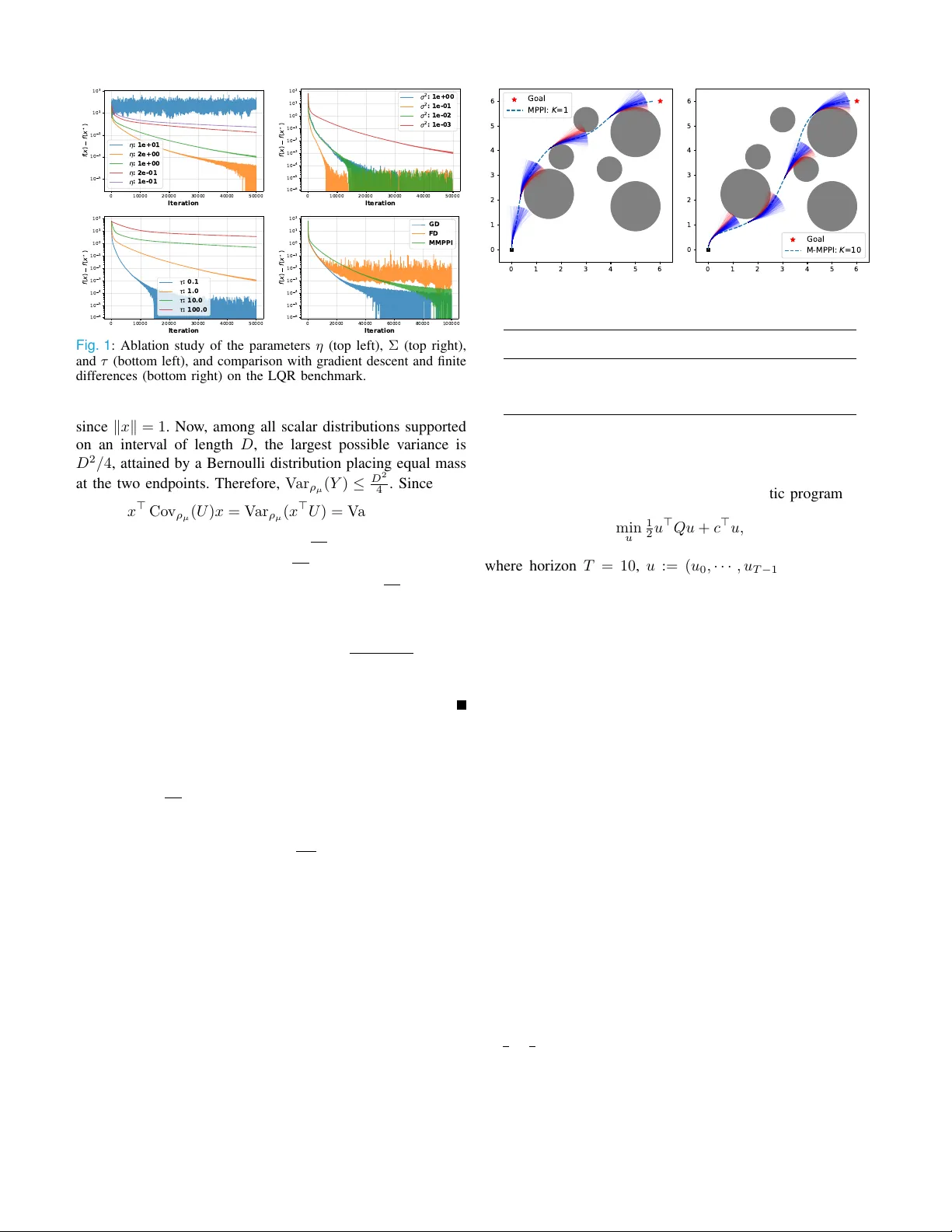
Model Predictiv e P ath Integr al Control as Preconditioned Gradient Descent Mah yar F azlyab , Sina Shar ifi, Jiarui W ang Abstract — Abstract — Model Predictive P ath Integral (MPPI) control is a popular sampling-based method for tra- jectory optimization in nonlinear and nonconve x settings, yet its optimization structure remains only partially un- derstood. We develop a variational, optimization-theoretic interpretation of MPPI by lifting constrained trajectory op- timization to a KL-regularized problem o ver distributions and reducing it to a negative log-par tition (free-energy) objective over a tractable sampling family . For a general parametric family , this yields a preconditioned gradient method on the distribution parameters and a natural multi- step extension of MPPI. For the fixed-co variance Gaussian family , we show that classical MPPI is recovered exactly as a preconditioned gradient descent step with unit step siz e. This interpretation enables a direct conver gence analysis: under bounded feasible sets, we derive an explicit upper bound on the smoothness constant and a simple sufficient condition guaranteeing descent of exact MPPI. Numerical experiments suppor t the theory and illustrate the effect of key h yperparameters on perf ormance. Index T erms — Optimal control, Optimization Algorithms, Predictive control f or nonlinear systems I . I N T R O D U C T I O N Model Predicti ve Path Integral (MPPI) control, e.g., [13, 15], is a widely used sampling-based method for trajectory optimization in nonlinear and noncon vex settings, owing to its simplicity , parallelizability , and ability to handle nondif- ferentiable dynamics and costs. In its standard form, MPPI updates the sampling distrib ution by drawing perturbed control sequences, reweighting them according to their trajectory costs, and shifting the nominal control to ward a weighted av erage of the sampled rollouts. Despite its empirical success in robotics and real-time control, this update is typically introduced through stochastic optimal control or control-as- inference arguments, which do not directly expose its underly- ing optimization structure. As a result, basic questions such as how MPPI relates to gradient-based methods, when its update is guaranteed to decrease a well-defined objective, and ho w its hyperparameters influence stability and con vergence remain only partially understood [4]. These gaps motiv ate the need for a direct optimization-theoretic interpretation of MPPI. The authors are with the Depar tment of Electr ical and Computer Engineering at Johns Hopkins University , Baltimore , MD 21218, USA. { mahyarfazlyab, sshari12, jwang486 } @jhu.edu A. Contributions This paper provides a v ariational, optimization-theoretic foundation for MPPI by reinterpreting it as stochastic opti- mization of a ne gative log-partition (free-ener gy) objective . W e lift constrained trajectory optimization to a KL-regularized problem over distributions and show that it reduces to min- imizing a free-energy objectiv e ov er a tractable sampling family . For a general parametric family , we derive exact gradient and Hessian formulas for the reduced objective and obtain a preconditioned gradient method on the parameters of the sampling distribution, leading naturally to a multi-step extension of MPPI. F or the fixed-co variance Gaussian family , we then show that classical MPPI is recovered exactly as a preconditioned gradient descent step with unit step size. This interpretation enables a direct conv ergence analysis; in particular , under bounded feasible sets, we derive an explicit upper bound on the smoothness constant and a simple suf- ficient condition guaranteeing descent of e xact MPPI with unit step size. Finally , we support the theory with numerical experiments on tw o trajectory optimization benchmarks: a linear–quadratic re gulator (LQR) problem and a Dubins car navigating a cluttered environment. While our emphasis is on trajectory optimization, the dev elopment is modular and applies more broadly to constrained sampling-based optimiza- tion. B. Related Work Probabilistic Inf erence P erspective: Inference-based formu- lations recast control as posterior inference ov er action se- quences conditioned on an optimality variable, leading to updates closely related to MPPI [4]. This viewpoint has been dev eloped extensi vely in reinforcement learning and control [6], and extended to model predictiv e control via variational inference [10]. In particular , [10] introduced a variational inference MPC frame work that reco vers se veral sampling- based optimization methods, including MPPI [14], CEM [1], and CMA-ES [2] as special cases. Our contribution is com- plementary: rather than deriving MPPI through inference, we show that it can be obtained directly as a preconditioned gradient step on a KL-regularized free-energy objectiv e. Diffusion P erspective: Another line of work connects MPPI to model-based diffusion [11, 16, 5]. In [16], building on the score estimation result from [11], that MPPI can be interpreted as performing score ascent on a Gaussian-smoothed Gibbs distribution. Although this interpretation explains the mecha- nism of MPPI, it still does not directly re veal its con vergence properties. Optimization P erspective: MPPI has also been related to optimization-based updates. For example, [7] showed that path integral policy improvement [12] can be viewed as mirror descent (MD) o ver trajectory distrib utions, where each update minimizes an expected cost regularized by a KL div ergence and leads to exponential reweighting. Building on this perspective, [9] proposed momentum and adapti ve step- size mechanisms to accelerate conv ergence. In practice, these MD updates must be projected onto a parametric family to retain tractable sampling and preserv e the structure of the distribution. For Gaussian families, the resulting algorithm recov ers standard MPPI. Theoretical Analysis of MPPI: Motiv ated by the empirical success of MPPI, se veral recent w orks have begun to study its theoretical properties. In particular, CoV O-MPC[17] analyzes the con vergence behavior of MPPI using contraction theory , proving at least linear con vergence for (time-varying) LQR. Howe ver , the contraction result cannot be extended to general nonlinear settings without making extra regularity assump- tions. Separately , [3] studies the optimality and suboptimality of MPPI in stochastic and deterministic settings, with an emphasis on deterministic MPPI and its approximation error . Our analysis is complementary to these works: we analyze the con vergence for general nonlinear systems and cost, with bounded feasible set being the main requirement. C . Notation For a symmetric matrix A , A ⪰ 0 and A ≻ 0 denote positi ve semidefiniteness and positive definiteness, respecti vely . The identity matrix is denoted by I , and λ min ( A ) , λ max ( A ) denote the extreme eigenv alues of A . The Euclidean norm and spectral norm are both denoted by ∥ · ∥ . For P ≻ 0 , we define ∥ x ∥ 2 P = x ⊤ P x and ∥ x ∥ 2 P − 1 = x ⊤ P − 1 x . For a probability density π , expectation, covariance, and support are denoted by E π [ · ] , Co v π ( · ) , and supp( π ) , respectiv ely . W e write π ( u ) = N ( u ; µ, Σ) , for a Gaussian density with mean µ and covariance Σ , and KL( ρ ∥ π ) for the Kullback–Leibler div ergence. For a dif ferentiable function F , ∇ F and ∇ 2 F denote its gradient and Hessian. For a set C ⊂ R d , we use 1 C ( u ) to denote its indicator function. I I . V A R I A T I O N A L F O R M U L A T I O N A. T r ajector y Optimization as Constrained Minimization W e consider finite-horizon trajectory optimization ov er an open-loop control sequence u := ( u 0 , u 1 , . . . , u T − 1 ) ∈ R dT applied to a dynamical system x t +1 = F ( x t , u t ) , possibly nonlinear and nonsmooth, from a giv en initial con- dition x 0 . Let f 0 ( u ) denote the trajectory objective (e.g., cumulativ e stage costs and a terminal cost), and let the feasible set be C := { u ∈ R dT : g i ( u ) ≤ 0 , i = 1 , . . . , m } , where the functions g i encode constraints such as obstacle av oidance and state bounds along the rollout, or input limits. The resulting trajectory optimization problem is min u ∈ C f 0 ( u ) . (1) Throughout, we assume that C ⊂ R dT is nonempty and compact, and that f 0 : R dT → R and g i : R dT → R , i = 1 , . . . , m , are continuous. Our goal is to lift (1) to an optimization problem over probability distributions supported on C , which will lead to a unifying v ariational interpretation of sampling-based trajectory optimization methods. B. KL-Regular ized Distr ibutional Formulation Follo wing the control-as-inference and KL-re gularized con- trol literature, we lift (1) to a distributional problem. Let ρ be a distribution ov er u representing the decision distribution , and let π be a base (or sampling) distribution. For a temperature τ > 0 , consider the KL-regularized objectiv e min ρ E ρ [ f 0 ( u )] + τ KL( ρ ∥ π ) s.t. supp( ρ ) ⊆ C, (2) where supp( ρ ) ⊆ C enforces hard feasibility . Problem (2) trades off expected cost under ρ with proximity to the base distribution π . In the limit τ → 0 , the regularization v anishes, and any optimal solution concentrates on the optimal set U ⋆ = arg min u ∈ C f 0 ( u ) . C . Optimizing the Base Distribution For an y fixed base distrib ution π , the KL-regularized prob- lem (2) provides an upper bound on the optimal value of the original constrained problem: min ρ  E ρ [ f 0 ( u )] + τ KL( ρ ∥ π )  ≥ min ρ E ρ [ f 0 ( u )] = min u ∈ C f 0 ( u ) , where both minimizations are taken over distributions ρ sup- ported on C , and the equality follows by choosing ρ as a Dirac measure at any minimizer of f 0 ov er C . This motiv ates optimizing over π in order to seek the tightest such upper bound. Howe ver , if we optimize over π without restriction, the pair ( ρ, π ) may collapse (e.g., π = ρ ), undermining stability and exploration. W e therefore restrict π to a tractable family Π (e.g., Gaussians with bounded covariance), and consider min π ∈ Π min ρ E ρ [ f 0 ( u )] + τ KL( ρ ∥ π ) s.t. supp( ρ ) ⊆ C. (3) This yields a principled formulation for optimizing the base distribution π . Specifically , for a fixed π ∈ Π , the minimizer ov er ρ in (3) is given by the truncated Gibbs tilt ρ ⋆ π ( u ) = T ( π )( u ) := π ( u ) exp  − f 0 ( u ) /τ  1 C ( u ) Z ( π ) , (4) where Z ( π ) is the normalizing constant Z ( π ) := Z C π ( v ) exp  − f 0 ( v ) /τ  dv (5) Substituting (4) into (3) yields the reduced problem min π ∈ Π − τ log Z ( π ) . (6) Thus, the original joint optimization over ( ρ, π ) reduces to the minimization of the neg ativ e log-partition function over the sampling family Π . I I I . O P T I M I Z A T I O N O V E R A P A R A M E T R I C S A M P L I N G F A M I L Y In this section, we specialize the reduced problem (6) to a parametric family of sampling distributions Π := { π θ : θ ∈ Θ } , where Θ ⊆ R p is the parameter space. For each θ ∈ Θ , the corresponding optimal decision distribution is ρ θ ( u ) := T ( π θ )( u ) . (7) Accordingly , the reduced problem becomes min θ ∈ Θ F ( θ ) := − τ log Z ( θ ) = − τ log Z C π θ ( u ) e − f 0 ( u ) τ du. (8) W e make the following assumption, under which the reduced objectiv e F becomes twice differentiable. Assumption 1: The family { π θ } θ ∈ Θ is strictly positive on C , twice continuously differentiable in θ , and such that differ - entiation under the integral sign is valid for Z ( θ ) up to second order . A. Preconditioned Gradient Descent In contrast to the original constrained trajectory optimiza- tion problem, the reduced problem (8) is differentiable in the distribution parameters and is therefore amenable to gradient- based optimization. The following result provides expressions for the gradient and Hessian of F ( θ ) that will be useful for algorithm design and con ver gence analysis. Lemma 1 (Gradient and Hessian Repr esentations): Under Assumption 1, ∇ F ( θ ) = − τ E ρ θ [ ∇ θ log π θ ( u )] (9) = − τ E π θ [ w ( u ) ∇ θ log π θ ( u )] E π θ [ w ( u )] , (10) where w ( u ) := exp  − f 0 ( u ) /τ  1 C ( u ) . (11) In addition, ∇ 2 F ( θ ) = − τ  E ρ θ  ∇ 2 θ log π θ ( u )  + Co v ρ θ ( ∇ θ log π θ ( u ))  . (12) Pr oof: See Section VII. The gradient representations in Lemma 1 naturally moti vate a preconditioned gradient method for minimizing the reduced objectiv e F ( θ ) . Gi ven a symmetric positive definite precondi- tioner P k ≻ 0 and a step size η k > 0 , the exact preconditioned gradient descent is θ k +1 = θ k − η k P k ∇ F ( θ k ) (13) = θ k + η k τ P k E ρ θ k [ ∇ θ log π θ k ( u )] . In practice, the expectation with respect to ρ θ k is generally intractable. Using (10), we can sample from π θ k instead. Specifically , we draw samples u ( j ) ∼ π θ k , j = 1 , . . . , N , and define the self-normalized importance weights ¯ w j := w ( u ( j ) ) P N r =1 w ( u ( r ) ) j = 1 , · · · , N . (14) Algorithm 1 Multi-step MPPI Require: Initial parameter θ 0 , number of samples N , number of iterations K 1: for k = 1 , · · · , K do ▷ K = 1 r ecovers MPPI 2: Sample u (1) , ..., u ( N ) i.i.d. ∼ π θ k − 1 ( u ) 3: Approximate ∇ θ F ( θ k ) according to (15). 4: Update θ k according to (16). 5: end for This yields the self-normalized Monte Carlo estimator of (10), [ ∇ θ F ( θ k ) = − τ N X j =1 ¯ w j ∇ θ log π θ k ( u ( j ) ) , (15) and the sampled preconditioned gradient update θ k +1 = θ k + η k τ P k N X j =1 ¯ w j ∇ θ log π θ k ( u ( j ) ) . (16) This update has the standard structure of a weighted sample av erage used in policy search and sampling-based control methods, and recov ers MPPI as a special case under a suitable Gaussian parameterization. B. Convergence Analysis W e now analyze the e xact preconditioned gradient iteration (13) with a constant step size η > 0 , and deriv e conditions under which it yields descent and con vergence of the reduced objectiv e. Since the iteration is preconditioned by P , the relev ant notion of smoothness is naturally expressed in the metric induced by P . Assumption 2: For the chosen positi ve definite matrix P ≻ 0 , there exists a constant L P > 0 such that sup θ ∈ Θ    P 1 / 2 ∇ 2 F ( θ ) P 1 / 2    ≤ L P . The following lemma is an immediate consequence of Assumption 2; its proof is given in Section VII. Lemma 2: Under Assumption 2, for all θ , θ + ∆ θ ∈ Θ , F ( θ + ∆ θ ) ≤ F ( θ ) + ∇ F ( θ ) ⊤ ∆ θ + L P 2 ∆ θ ⊤ P − 1 ∆ θ . (17) Theor em 1: Suppose Assumption 2 holds, and let { θ k } be generated by (13) with a constant step size η > 0 . If 0 < η < 2 L P , (18) then the following hold: 1) Descent: for every k , F ( θ k +1 ) ≤ F ( θ k ) − η  1 − η L P 2  ∥∇ F ( θ k ) ∥ 2 P . (19) 2) Summability of preconditioned gradients: ∞ X k =0 ∥∇ F ( θ k ) ∥ 2 P ≤ F ( θ 0 ) − inf θ ∈ Θ F ( θ ) η  1 − η L P 2  . (20) 3) Stationarity: for every K ≥ 1 , min 0 ≤ j ≤ K − 1 ∥∇ F ( θ j ) ∥ 2 P ≤ F ( θ 0 ) − inf θ ∈ Θ F ( θ ) K η  1 − η L P 2  . (21) In particular, lim k →∞ ∥∇ F ( θ k ) ∥ P = 0 . Pr oof: Applying the smoothness bound (17) with ∆ θ = − η P ∇ F ( θ k ) , we obtain (19) after simplification. Since 0 < η < 2 /L P , the coefficient is positiv e, so F ( θ k ) is nonin- creasing. Summing (19) from k = 0 to K − 1 and using inf θ ∈ Θ F ( θ ) ≤ F ( θ K ) η  1 − η L P 2  K − 1 X k =0 ∥∇ F ( θ k ) ∥ 2 P ≤ F ( θ 0 ) − inf θ ∈ Θ F ( θ ) . Letting K → ∞ giv es (20). Dividing by K giv es (21), and summability implies ∥∇ F ( θ k ) ∥ P → 0 . I V . O P T I M I Z ATI O N OV E R G AU S S I A N F A M I L Y W I T H F I X E D C O VA R I A N C E W e now specialize the preceding results to the fixed- cov ariance Gaussian family π µ ( u ) = N ( u ; µ, Σ) , Σ ≻ 0 , (22) where the mean µ ∈ R m is the optimization variable. In this case, the score and log-Hessian are giv en by ∇ µ log π µ ( u ) = Σ − 1 ( u − µ ) , ∇ 2 µ log π µ ( u ) = − Σ − 1 . Substituting these expressions into Lemma 1 yields ∇ F ( µ ) = − τ Σ − 1  E ρ µ [ u ] − µ  , ρ µ ( u ) = T ( π µ )( u ) . (23) Using (23), the exact preconditioned gradient step (13) be- comes µ k +1 = µ k + η k τ P k Σ − 1  E ρ µ k [ u ] − µ k  . (24) Using the ratio-of-expectations representation in (10), the expectation E ρ µ k [ u ] can be approximated by self-normalized importance sampling. Accordingly , if u ( j ) ∼ N ( µ k , Σ) and the normalized weights ¯ w j are defined as in (14), a Monte Carlo implementation of (24) is µ k +1 = µ k + η k τ P k Σ − 1   N X j =1 ¯ w j u ( j ) − µ k   . (25) A. MPPI as a Special Case For the fixed-cov ariance Gaussian family , choose P k = 1 τ Σ , η k = 1 . Then the e xact preconditioned gradient update (24) reduces to µ k +1 = E ρ µ k [ u ] = E π µ k [ w ( u ) u ] E π µ k [ w ( u )] , (26) where w ( u ) = exp( − f 0 ( u ) /τ ) 1 C ( u ) , and the last equality follows from the ratio-of-expectations in Lemma 1. Corre- spondingly , the Monte Carlo implementation becomes µ k +1 = N X j =1 ¯ w j u ( j ) , u ( j ) ∼ N ( µ k , Σ) , (27) which is precisely the classical MPPI update. B. Convergence analysis W e now analyze the exact Gaussian update (24) through the lens of preconditioned gradient descent. Although (24) is well defined for any positive definite preconditioner P k , the choice P k = 1 τ Σ is especially natural for two reasons. First, when η k = 1 , this choice exactly recovers the classical MPPI update, as shown in the previous subsection. Therefore, con ver gence guarantees established under P = Σ /τ immediately apply to MPPI, as well as to its relaxed version with arbitrary step size η k > 0 . Second, this preconditioner is intrinsic to the geometry of the fixed-co variance Gaussian family . Indeed, by Lemma 1, ∇ 2 F ( µ ) = τ Σ − 1 − τ Σ − 1 Co v ρ µ ( u )Σ − 1 . Hence, with P = Σ /τ , P 1 / 2 ∇ 2 F ( µ ) P 1 / 2 =  Σ τ  1 / 2 ∇ 2 F ( µ )  Σ τ  1 / 2 (28) = I − Σ − 1 / 2 Co v ρ µ ( u )Σ − 1 / 2 . Thus, in the metric induced by P = Σ /τ , the curv ature of the reduced objective is determined entirely by the cov ariance of the tilted distribution ρ µ relativ e to the sampling covariance Σ . In particular, the explicit dependence on the temperature τ disappears after preconditioning. This makes P = Σ /τ the natural scaling for the con vergence analysis. Accordingly , throughout this subsection we specialize (24) to the update µ k +1 = (1 − η k ) µ k + η k E ρ µ k [ u ] , (29) which we refer to as the exact r elaxed MPPI update . T o state the conv ergence result, define L Σ := sup µ ∈ Θ    I − Σ − 1 / 2 Co v ρ µ ( u )Σ − 1 / 2    . (30) By (28), L Σ is the operator-norm bound on the Hessian of F in the metric induced by Σ /τ , and hence the corresponding smoothness constant in that metric. In the next theorem, we state the con ver gence result for (29). Theor em 2: Consider the fixed-cov ariance Gaussian family (22), and the exact preconditioned gradient update (24). As- sume that the feasible set C ⊂ R m is bounded, with diameter D := sup u,v ∈ C ∥ u − v ∥ . Then the metric smoothness constant (30) satisfies L Σ ≤ max  1 , D 2 4 λ min (Σ) − 1  . (31) Consequently , the exact relaxed MPPI update (29) satisfies the descent and con ver gence conclusions of Theorem 1 whenever 0 < η k < 2 L Σ . Pr oof: Define the 1D random v ariable Y = x ⊤ U , where U ∼ ρ µ and x ∈ R n is a unit vector . Since ρ µ is supported on C , Y has a support interval of length at most D . Indeed, sup u,v ∈ C | x ⊤ u − x ⊤ v | ≤ sup u,v ∈ C ∥ x ∥ ∥ u − v ∥ ≤ D , 0 10000 20000 30000 40000 50000 Iteration 1 0 5 1 0 3 1 0 1 1 0 1 1 0 3 f ( x ) f ( x ) : 1 e + 0 1 : 2 e + 0 0 : 1 e + 0 0 : 2 e - 0 1 : 1 e - 0 1 0 10000 20000 30000 40000 50000 Iteration 1 0 6 1 0 5 1 0 4 1 0 3 1 0 2 1 0 1 1 0 0 1 0 1 1 0 2 f ( x ) f ( x ) 2 : 1 e + 0 0 2 : 1 e - 0 1 2 : 1 e - 0 2 2 : 1 e - 0 3 0 10000 20000 30000 40000 50000 Iteration 1 0 6 1 0 5 1 0 4 1 0 3 1 0 2 1 0 1 1 0 0 1 0 1 1 0 2 f ( x ) f ( x ) : 0 . 1 : 1 . 0 : 1 0 . 0 : 1 0 0 . 0 0 20000 40000 60000 80000 100000 Iteration 1 0 6 1 0 5 1 0 4 1 0 3 1 0 2 1 0 1 1 0 0 1 0 1 1 0 2 f ( x ) f ( x ) GD FD MMPPI Fig. 1 : Ablation study of the parameters η (top left), Σ (top right), and τ (bottom left), and comparison with gradient descent and finite differences (bottom right) on the LQR benchmark. since ∥ x ∥ = 1 . Now , among all scalar distributions supported on an interval of length D , the largest possible v ariance is D 2 / 4 , attained by a Bernoulli distrib ution placing equal mass at the two endpoints. Therefore, V ar ρ µ ( Y ) ≤ D 2 4 . Since x ⊤ Co v ρ µ ( U ) x = V ar ρ µ ( x ⊤ U ) = V ar ρ µ ( Y ) , it follows that x ⊤ Co v ρ µ ( U ) x ≤ D 2 4 for ev ery unit vec- tor x . Hence, Cov ρ µ ( U ) ⪯ D 2 4 I . Next, define A = Σ − 1 / 2 Co v ρ µ ( u )Σ − 1 / 2 . Then we hav e 0 ⪯ A ⪯ D 2 4 Σ − 1 .Now , using the inequality ∥ I − A ∥ ≤ max(1 , λ max ( A ) − 1) , we obtain    I − Σ − 1 / 2 Co v ρ µ ( u )Σ − 1 / 2    ≤ max { 1 , D 2 4 λ min (Σ) − 1 } . T aking the supremum ov er µ prov es (31). The step-size condition then follows directly from Theorem 1. Implication f or MPPI with unit step size: The exact MPPI iteration is recovered by setting η k = 1 in (29). Hence, con- ver gence of the e xact MPPI iteration follo ws from Theorem 2 whenev er the unit step size satisfies the admissibility condition for 0 < 1 < 2 L Σ , which is equiv alent to L Σ < 2 . Using the bound in (31), a sufficient condition is therefore λ min (Σ) > D 2 12 . Thus, if the cov ariance matrix is sufficiently large, then the exact MPPI iteration with η = 1 satisfies the descent and con vergence guarantees of Theorem 1. In particular , this gi ves a simple design rule: the exploration covariance must not be too small relativ e to the diameter of the feasible set. Equiv alently , overly concentrated sampling distributions can destroy the global descent guarantee, whereas sufficiently diffuse sampling is enough to ensure it. V . N U M E R I C A L A N A L Y S I S A. Linear Quadratic Regulator (LQR) W e consider a finite-horizon LQR trajectory optimization problem with double-integrator dynamics x t +1 =  1 1 0 1  x t +  0 . 5 1  u t . 0 1 2 3 4 5 6 0 1 2 3 4 5 6 Goal M P P I : K = 1 0 1 2 3 4 5 6 0 1 2 3 4 5 6 Goal M - M P P I : K = 1 0 Fig. 2 : Comparison of the trajectories chosen by MPPI and 10-step MPPI on the Dubins car benchmark in a cluttered en vironment. Runtime Sample acceptance A verage (s) rate % cost MPPI ( K = 1 ) 16.8 0.75 26.14 Log-MPPI 17.1 0.75 24.3 M-MPPI ( K = 5 ) 34.4 0.79 23.98 M-MPPI ( K = 10 ) 47.8 0.80 23.85 T ABLE I : Comparison of runtime, sample acceptance rate % , and av erage cost of the chosen trajectory for v arious methods. Rolling out the trajectories yields the quadratic program min u 1 2 u ⊤ Qu + c ⊤ u, where horizon T = 10 , u := ( u 0 , · · · , u T − 1 ) ∈ R 10 is the stacked control vector , x 0 = (2 . 5 , 0) , and Q ⪰ 0 and c can be computed as discussed in [17]. W e set a budget of N = 5 samples per iteration. Figure 1 shows the results for different choices of η , τ , and Σ = σ 2 I . The figures show that, up to some threshold, increasing the η and σ 2 improv es the con vergence. This is expected because the term η P = η σ 2 /τ acts as the step size. W e also compare Multi-step MPPI (M- MPPI) with gradient descent (GD) and finite differences (FD). B. Dubins Car W e then consider a trajectory optimization task in a cluttered en vironment, where a Dubins car must reach a given destina- tion. At each time, the optimization problem is formulated as min u ∈C T X t =1 ∥ x t − x d ∥ 2 Q + ∥ u t ∥ 2 R , where T = 20 , Q = diag(1 , 1 , 0 . 01) , R = 0 . 001 , x 0 = (0 , 0 , π / 2) , and x d = (6 , 6 , 0) . The system dynamics x t = [ p x t , p y t , θ t ] ⊤ are x t +1 = x t + [ v cos( θ t ) , v sin( θ t ) , w t ] ⊤ ∆ t, where v = 4 is the constant velocity and the control w t ∈ [ − 3 2 π , 3 2 π ] , and we set N = 1024 . Figure 2 shows the trajectory chosen by the algorithm with K = 1 (MPPI) and K = 10 . Since MPPI does not iterate until con vergence, it selects a suboptimal path. More details on this setup and comparison with Log-MPPI [8] are in T able I, where we show that increasing K improv es the av erage cost, at the expense of runtime. The reported results are averaged ov er 3 seeds. V I . C O N C L U S I O N This paper showed that MPPI admits a direct v ariational and optimization-theoretic interpretation. By lifting constrained trajectory optimization to a KL-regularized problem over distributions, we obtained a free-energy objective whose opti- mization ov er a parametric sampling family yields a precon- ditioned gradient method. In the Gaussian fixed-co variance setting, this recovers classical MPPI exactly and leads to explicit descent and stationarity guarantees, as well as a simple cov ariance-dependent design rule for unit-step MPPI. These results help demystify MPPI from an optimization viewpoint and open the door to principled extensions of sampling-based control methods. V I I . A P P E N D I X Proof of Lemma 1: Differentiating Z ( θ ) = E π θ [ e − f 0 ( u ) /τ ] with respect to θ , using the identity ∇ θ π θ ( u ) = π θ ( u ) ∇ θ log π θ ( u ) , and dividing both sides by Z ( θ ) yields ∇ θ log Z ( θ ) = Z C ∇ θ log π θ ( u ) π θ ( u ) e − f 0 ( u ) /τ Z ( θ ) du = E ρ θ [ ∇ θ log π θ ( u )] . Since F ( θ ) = − τ log Z ( θ ) , we obtain (9) and get (10) using (11). Next, we compute the Hessian of F ( θ ) . Differentiating (10) with respect to θ gives ∇ 2 θ F ( θ ) = − τ ∇ θ E π θ [ w ( u ) ∇ θ log π θ ( u )] E π θ [ w ( u )] . (32) Since ρ θ ( u ) depends on θ through π θ ( u ) and Z ( θ ) , we dif fer- entiate the expectation using the quotient rule. Define A ( θ ) = E π θ [ w ( u ) ∇ θ log π θ ( u )] , B ( θ ) = E π θ [ w ( u )] . From (10) we hav e ∇ θ F ( θ ) = − τ A ( θ ) B ( θ ) . Dif ferentiating this e xpression yields ∇ 2 θ F ( θ ) = − τ  ∇ θ A ( θ ) B ( θ ) − A ( θ ) ∇ θ B ( θ ) ⊤ B ( θ ) 2  . (33) W e first compute ∇ θ B ( θ ) . Using the score identity , ∇ θ B ( θ ) = ∇ θ E π θ [ w ( u )] = E π θ [ w ( u ) ∇ θ log π θ ( u )] = A ( θ ) . Next, differentiating A ( θ ) and again using differentiation of expectations under π θ giv es ∇ θ A ( θ ) = E h w ( u )  ∇ 2 θ log π θ ( u ) + ∇ θ log π θ ( u ) ∇ θ log π θ ( u ) ⊤ i . Substituting these expressions into (33) and writing the result in terms of the distribution ρ θ yields (12). Proof of Lemma 2 By T aylor’ s theorem with integral remainder , F ( θ + ∆ θ ) = F ( θ ) + ∇ F ( θ ) ⊤ ∆ θ + Z 1 0 (1 − t ) ∆ θ ⊤ ∇ 2 F ( θ + t ∆ θ )∆ θ | {z } M dt. For any t ∈ [0 , 1] and P ≻ 0 , M = ∆ θ ⊤ P − 1 / 2 P 1 / 2 ∇ 2 F ( θ + t ∆ θ ) P 1 / 2 P − 1 / 2 ∆ θ ≤ ∥ P 1 / 2 ∇ 2 F ( θ + t ∆ θ ) P 1 / 2 ∥ ∆ θ ⊤ P − 1 ∆ θ ≤ L P ∆ θ ⊤ P − 1 ∆ θ . Substituting this bound and using R 1 0 (1 − t ) dt = 1 2 yields (17). R E F E R E N C E S [1] Zdravk o I Botev et al. “The cross-entropy method for opti- mization”. In: Handbook of statistics . V ol. 31. Else vier , 2013, pp. 35–59. [2] Nikolaus Hansen, Sibylle D M ¨ uller, and Petros K oumout- sakos. “Reducing the time complexity of the derandomized ev olution strategy with cov ariance matrix adaptation (CMA- ES)”. In: Evolutionary computation 11.1 (2003), pp. 1–18. [3] Hannes Homburger et al. “Optimality and suboptimality of MPPI control in stochastic and deterministic settings”. In: IEEE Contr ol Systems Letters (2025). [4] K ohei Honda. “Model Predictiv e Control via Probabilistic Inference: A T utorial”. In: arXiv pr eprint (2025). [5] W onsuhk Jung et al. “Joint Model-based Model-free Dif- fusion for Planning with Constraints”. In: arXiv pr eprint arXiv:2509.08775 (2025). [6] Serge y Levine. “Reinforcement learning and control as prob- abilistic inference: Tutorial and review”. In: arXiv pr eprint arXiv:1805.00909 (2018). [7] Megumi Miyashita, Shiro Y ano, and T oshiyuki Kondo. “Mir- ror descent search and its acceleration”. In: Robotics and Autonomous Systems 106 (2018), pp. 107–116. [8] Ihab S Mohamed, Kai Yin, and Lantao Liu. “Autonomous navigation of agvs in unknown cluttered environments: log- mppi control strategy”. In: IEEE Robotics and A utomation Letters 7.4 (2022), pp. 10240–10247. [9] Masashi Okada and T adahiro T aniguchi. “ Acceleration of gradient-based path integral method for efficient optimal and in verse optimal control”. In: 2018 IEEE International Con- fer ence on Robotics and A utomation (ICRA) . IEEE. 2018, pp. 3013–3020. [10] Masashi Okada and T adahiro T aniguchi. “V ariational infer- ence mpc for bayesian model-based reinforcement learning”. In: Conference on r obot learning . PMLR. 2020, pp. 258–272. [11] Chaoyi Pan et al. “Model-based diffusion for trajectory op- timization”. In: Advances in Neural Information Pr ocessing Systems 37 (2024), pp. 57914–57943. [12] Evangelos Theodorou, Jonas Buchli, and Stefan Schaal. “Re- inforcement learning of motor skills in high dimensions: A path integral approach”. In: 2010 IEEE International Con- fer ence on Robotics and Automation . IEEE. 2010, pp. 2397– 2403. [13] Grady W illiams, Andrew Aldrich, and Evangelos Theodorou. “Model predictiv e path integral control using cov ari- ance variable importance sampling”. In: arXiv preprint arXiv:1509.01149 (2015). [14] Grady Williams et al. “ Aggressiv e driving with model pre- dictiv e path integral control”. In: 2016 IEEE international confer ence on r obotics and automation (ICRA) . IEEE. 2016, pp. 1433–1440. [15] Grady Williams et al. “Information theoretic MPC for model- based reinforcement learning”. In: 2017 IEEE international confer ence on r obotics and automation (ICRA) . IEEE. 2017, pp. 1714–1721. [16] Haoru Xue et al. “Full-order sampling-based mpc for torque- lev el locomotion control via diffusion-style annealing”. In: 2025 IEEE International Conference on Robotics and Au- tomation (ICRA) . IEEE. 2025, pp. 4974–4981. [17] Zeji Y i et al. “CoVO-MPC: Theoretical analysis of sampling- based MPC and optimal covariance design”. In: 6th Annual Learning for Dynamics & Contr ol Conference . PMLR. 2024, pp. 1122–1135.