Conformalized Transfer Learning for Li-ion Battery State of Health Forecasting under Manufacturing and Usage Variability

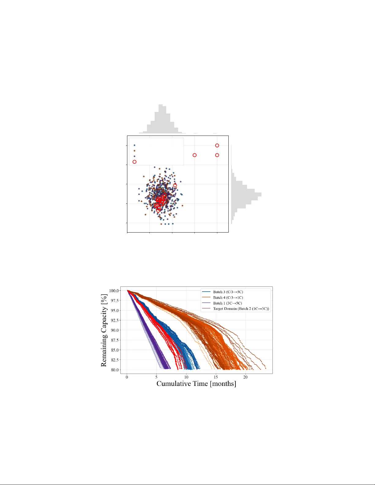
Conf ormalized T ransfer Lear ning f or Li-ion Battery State of Health F or ecasting under Manufacturing and Usage V ariability A P R E P R I N T Samuel Filgueira da Silv a 1 , Mehmet Fatih Ozkan 1 , Faissal El Idrissi 1 , and Marcello Canov a 1 1 Department of Mechanical and Aerospace Engineering, Center for Automotiv e Research, The Ohio State Univ ersity , Columb us, OH, USA filgueiradasilva.1@osu.edu, ozkan.25@osu.edu, elidrissi.2@osu.edu, canova.1@osu.edu March 26, 2026 Abstract Accurate forecasting of state-of-health (SOH) is essential for ensuring safe and reliable operation of lithium-ion cells. Howe ver , existing models calibrated on laboratory tests at specific conditions often fail to generalize to ne w cells that differ due to small manufacturing v ariations or operate under different conditions. T o address this challenge, an uncertainty-aw are transfer learning frame work is proposed, combining a Long Short-T erm Memory (LSTM) model with domain adaptation via Maximum Mean Discrepancy (MMD) and uncertainty quantification through Conformal Prediction (CP). The LSTM model is trained on a virtual battery dataset designed to capture real-world variability in electrode manufacturing and operating conditions. MMD aligns latent feature distrib utions between simulated and target domains to mitigate domain shift, while CP provides calibrated, distrib ution-free prediction intervals. This framework impro ves both the generalization and trustworthiness of SOH forecasts across heterogeneous cells. 1 Intr oduction Lithium-ion batteries play a dominant role in the transition to ward electrified transportation and rene wable energy integration, although their limited lifespan remains a critical technological bottleneck. Accurate prediction of the battery state of health (SOH) is essential not only for ensuring safety and reliability , but also for enabling advanced energy management strategies such as aging-aware fast charging [ 1 ]. Despite their importance, capturing SOH trajectories ov er long horizons remains challenging due to the complex, nonlinear , and often coupled nature of degradation mechanisms [2]. Physics-based models, such as the Pseudo-T wo-Dimensional (P2D) and Extended Single Particle Model (ESPM), provide v aluable insights into electrochemical processes and can be augmented with degradation submodels such as solid electrolyte interphase (SEI) gro wth, lithium plating, and loss of acti ve material [ 3 ]. These models hav e the advantage of interpretability and can simulate aging under di verse operating conditions [4]. Recent studies hav e also shown that deep learning (DL) models can effecti vely uncover nonlinear mappings between usage patterns and degradation outcomes [ 5 ]. Howe ver , data-dri ven models face challenges in terms of rob ustness when applied to pre viously unseen conditions. One of the critical challenges arises from cell-to-cell variability [ 6 ], where ev en minor deviations in electrode manufacturing can yield significant changes in degradation behavior [ 7 ]. Traditional SOH forecasting models are generally trained on nominal 1 cells, limiting their ability to generalize to samples that de viate from the av erage population. Consequently , there is a need for modeling approaches that can effecti vely le verage kno wledge from a generic population of cells while transferring it to non-nominal cases. T ransfer learning (TL) has emerged as a strategy to address this issue. By transferring knowledge from a well-characterized source domain to a less-represented target domain, TL enables robust forecasting under distribution shifts, such as variations in temperature, cycling rates, and cell configurations. Recent works ha ve employed TL-assisted SOH forecasting, using fine-tuning [ 8 ], metric-based domain adaptation techniques [ 9 , 10 ] based on Maximum Mean Discrepanc y (MMD) and Correlation Alignment (CORAL), and adversarial approaches such as Domain-Adversarial Neural Networks (D ANNs) [ 11 , 12 ]. These methods hav e demonstrated improved generalization across operating conditions, b ut limited attention has been given to TL across cell-to-cell v ariability caused by manufacturing processes. Another ke y challenge is quantifying the reliability of predictions. Existing approaches to uncertainty quantification (UQ), including Bayesian deep learning [ 13 ], Gaussian processes [ 14 ], and Monte Carlo dropout [ 15 ], often rely on distrib utional assumptions that lead to ov erconfident estimates under real-world v ariability . This paper proposes an uncertainty-aware, data-dri ven frame work for SOH forecasting that addresses v ariability induced by manufacturi ng processes and operating conditions. The approach inte grates an LSTM model with domain-adapti ve transfer learning to improv e generalization, while incorporating Conformal Prediction (CP) to provide distrib ution-free, finite-sample uncertainty quantification. The ke y contributions of this work are the de velopment of a transfer learning framew ork that enables SOH forecasting across cells with manufacturing and usage-induced v ariability , and the integration of CP to deliv er calibrated uncertainty interv als under variable and data-scarce conditions. 2 Over view of LiB Cell Model Equations This study adopts the Single Particle Model with electrolyte (SPMe) implemented in PyBaMM. SPMe extends the traditional Single P article Model by including electrolyte concentration and potential dynamics, improving v oltage prediction under high C-rates. For bre vity , the full set of gov erning equations is omitted here and can be found in [16]. The terminal voltage is expressed as: V SPMe ( t ) = U p ( c s , p , t ) − U n ( c s , n , t ) −  η p ( 0 , t ) − η n ( L , t )  −  φ e ( 0 , t ) − φ e ( L , t )  − I ( t ) R c , (1) where U i are the electrode open-circuit potentials, η i the kinetic ov erpotentials, φ e the electrolyte potential, c s , i the solid-phase lithium concentration (with i = n , p ), and R c the lumped contact resistance. 2.1 Battery Degradation Model T o capture long-term capacity fade and performance loss, the SPMe is augmented with degradation submodels for loss of active material (LAM) and loss of lithium in ventory (LLI) dri ven by SEI gro wth. The adopted formulations are consistent with physics-based capacity-loss models for graphite anodes and SEI/LAM mechanisms reported in the literature [ 3 , 17 ]. The model has pre viously been calibrated and v alidated against experimental capacity-f ade datasets for an A123 26650 cell [18], supporting its use for SOH prediction. 2.1.1 Loss of Active Material LAM accounts for the progressive deacti v ation of electrochemically acti ve particles due to mechanical stress, electrode cracking, or reactions that isolate activ e material. It is modeled as a time-dependent decrease in the 2 acti ve material volume fraction ε AM , i of electrode i ∈ { n , p } : d ε AM , i d t = − k AM , i 3 R i ε AM , i A L i   I ( t )   exp  − E AM , i RT  , (2) where ε AM , i is the acti ve-material volume fraction, R i the particle radius, L i the electrode thickness, A the electrode area, I ( t ) the applied current, and k AM , i and E AM , i empirical parameters. Decreasing ε AM , i reduces the av ailable cyclable capacity of the corresponding electrode. 2.1.2 SEI Layer Gr owth Lithium loss due to the SEI layer gro wth is produced by the side reaction at the anode caused by the ethylene carbonate (EC) reduction in the or ganic electrolyte compounds. The formation of SEI consumes c yclable lithium, reducing the in ventory av ailable for intercalation. F ollowing [ 19 ], the side reaction current density is modeled using a cathodic T afel e xpression: i s = − F k f , s c EC exp  − β s F RT ( Φ 1 − R SEI i t )  , (3) where i s is the side-reaction current density [A/m 2 ], k f , s the rate constant [m/s], c EC the solvent concentration in the SEI film [mol/m 3 ], Φ 1 the neg ativ e-electrode solid-phase potential [V], R SEI the SEI film resistance [ Ω · m 2 ], and i t the total interf acial current density [A/m 2 ]. T ogether , Eqs. (2) – (3) extend the SPMe with capacity-fade pathways capturing both electrode material degradation (LAM) and lithium in ventory loss due to side reactions (LLI). 3 Methodology 3.1 Generation and Prepr ocessing of Synthetic Aging Data T o emulate the ef fects of manufacturing v ariability on battery aging, synthetic datasets were generated for a 30 Ah nickel–manganese–cobalt (NMC) graphite cell using the PyBaMM en vironment [ 20 ]. In particular , cell-to-cell heterogeneity was introduced by varying the acti ve material v olume fractions of the positive and negati ve electrodes, parameters kno wn to strongly influence capacity fade signatures [ 6 , 7 ]. For each batch, applied C-rates v ary randomly e very 1 kAh throughput within their predefined operating ranges (T able 1). Additionally , each full cycle is simulated at 100% depth-of-discharge (DoD) and ambient temperature of 298K. T able 1: C-rate operating sets for each batch Batch C-rate Operating Set Batch 1 ( B 1 ) {3C, 4C, 5C} Batch 2 ( B 2 ) {1C, 2C, 3C} Batch 3 ( B 3 ) {C/3, C/2, 1C, 2C, 3C, 4C, 5C} Batch 4 ( B 4 ) {C/3, C/2, 1C} 3.1.1 Source and T arget Domain Selection In batches 1, 3 and 4 (source domain), virtual cells were created by sampling negati ve and positiv e electrode acti ve material v olume fractions from a Gaussian distribution centered on nominal values, with standard 3 de viations chosen to span ± 5% of the mean. Each sampled pair of ( ε s , n , ε s , p ) v alues corresponds to a distinct synthetic cell, producing unique SOH degradation trajectories. On the other hand, batch 2 (tar get domain) presents dif ferent discharge/charge protocols with ( ε s , n , ε s , p ) v alues in and out of the distribution (Fig. 1). Battery cycling and de gradation simulations were executed in parallel using a 20-core computing setup, enabling ef ficient large-scale data generation. The resulting dataset contains di verse degradation behaviors across batches and cell populations, as sho wn in Figs. 1-2. 0.38 0.40 0.42 0.44 0.46 Anode Volume Fraction ( ε s , n ) 0.56 0.58 0.60 0.62 0.64 Cathode Volume Fraction ( ε s , p ) Batches Batch 3 (C/3→5C) Batch 4 (C/3→1C) Batch 1 (3C→5C) T arget, Batch 2 (1C→3C) 1 2 3 Figure 1: Joint distrib ution of negati ve and positi ve electrode activ e material volume fractions across batches. Figure 2: SOH trajectories for each batch. 4 3.1.2 F eature Selection In this study , the feature set is constrained to reflect the realistic av ailability of information in the target domain. Specifically , it is assumed that be yond a cutoff point of 20 kAh throughput, detailed battery beha vior such as voltage profiles, dif ferential capacity ( d Q / dV ) shifts, or other electrochemical signatures are not accessible. This assumption reflects practical limitations in real-w orld scenarios, where only limited diagnostic data may be collected from ne w or anomalous cells. Consequently , these observ ables were not considered as input features for reconstructing the SOH trajectories. Instead, only discharge/charge C-rate protocols (the primary features that remain consistently measurable across both source and tar get domains) will be used for SOH forecasting. 3.2 Conf ormalized Deep T ransfer Learning Strategy 3.2.1 Deep Learning Ar chitecture Selection In this study , a Long Short-T erm Memory (LSTM) architecture was adopted to address the vanishing gradient issues that typically hinder recurrent neural networks (RNNs) in learning long-term dependencies [ 21 ]. LSTMs incorporate gating mechanisms that enable them to capture temporal correlations in battery degradation data, allo wing the model to learn comple x nonlinear relationships between usage patterns and state of health ov er extended horizons. 3.2.2 T ransfer Learning Framew ork The proposed transfer learning (TL) frame work is illustrated in Fig. 3. The source domain D s contains a lar ge set of fully labeled cells: 1   =    ,    𝑐    ∈ ℝ  D e n s e L a ye r 𝑺 𝑶𝑯 𝒌 + 𝟏 𝑆 𝑂 𝐻 𝑘 − 𝑤 + 1 ,  𝑘 − 𝑤 + 1 , … , 𝑆 𝑂 𝐻 𝑘 ,  𝑘 L ST M E n c o d e r D e c o d e r S O U R C E D e n s e L a ye r 𝑺 𝑶𝑯 𝒌 + 𝟏 𝑆 𝑂 𝐻 𝑘 − 𝑤 + 1 ,  𝑘 − 𝑤 + 1 , … , 𝑆 𝑂 𝐻 𝑘 ,  𝑘 L ST M E n c o d e r D ec o d er T AR G ET     We i g h t s h a re     Figure 3: Proposed transfer learning framework combining LSTM-based encoder–decoder with MMD-based domain adaptation. D s =  x s , y s  (4) 5 whereas the target domain D t consists of a limited number of labeled samples (av ailable until the 20 kAh cutof f) and a larger set of unlabeled samples: D t =  x t , y t  ∪  x t  u (5) Each input sample x k represents a sequence of w past time steps (sliding windo w): x k =  SOH k − w + 1 , u k − w + 1 , . . . , SOH k , u k  (6) with u k = [ I dis k , I ch k ] denoting the discharge/char ge C-rates, and y k = SOH k + 1 being the one-step-ahead label. Latent representation and decoder output The LSTM encoder maps the input sequence into a latent representation: z k = G ( x k ; θ ) (7) where G θ denotes the encoder parameterized by θ . The decoder takes z k as input and produces the hidden state: h k = H ( z k ; ψ ) (8) where H represents the decoder transformation with parameters ψ . The SOH prediction is then obtained via a dense (fully connected) layer: d SOH k + 1 = F ( h k ; ω ) (9) where ω are the predictor weights. Domain adaptation. T o mitigate the distrib ution shift between source and target domains, Maximum Mean Discrepancy (MMD) is used to align the latent representations z s k and z t k in a reproducing kernel Hilbert space (RKHS): MMD ( z s , z t ) =      1 n s n s ∑ i = 1 φ ( z s i ) − 1 n t n t ∑ j = 1 φ ( z t j )      2 H (10) Using the kernel trick, the squared MMD can be e xpressed as: MMD 2 ( z s , z t ) = 1 n 2 s n s ∑ i = 1 n s ∑ j = 1 k ( z s i , z s j ) + 1 n 2 t n t ∑ i = 1 n t ∑ j = 1 k ( z t i , z t j ) − 2 n s n t n s ∑ i = 1 n t ∑ j = 1 k ( z s i , z t j ) (11) where k ( · , · ) is chosen as a Gaussian kernel: k ( z s i , z t j ) = exp − ∥ z s i − z t j ∥ 2 2 σ 2 ! (12) Joint optimization The netw ork is trained by minimizing a combined loss function: L total ( θ , ψ , ω ) = ∑ i ∈ D s  SOH i − d SOH i  2 | {z } L source ( θ , ψ , ω ) + λ MMD  z s , z t  | {z } L MMD ( θ ) , (13) where λ acts as a re gularization coefficient balancing prediction accurac y and domain alignment. T o select an appropriate v alue for λ without relying on tar get-domain labels, a Leave-One-Batch-Out (LOBO) cross- v alidation procedure is performed entirely within the source domain. In this approach, one batch of source data is withheld during training and used as a pseudo-target domain to ev aluate the domain adaptation 6 performance, as described in Algorithm 1. The hyperparameter λ is then chosen to minimize the validation error across all LOBO folds. The optimal model parameters are obtained by solving: θ ∗ , ψ ∗ , ω ∗ = arg min θ , ψ , ω L total ( θ , ψ , ω ) (14) Algorithm 1 LOBO for the MMD weight λ tuning 1: Input: Λ = { λ 1 , ..., λ K } ⊂ [ 0 , 1 ] , batches { B 1 , . . . , B B } 2: Output: λ ⋆ 3: for λ ∈ Λ do 4: scores ← [ ] 5: f or b = 1 to B do ▷ sweeping all source batches 6: D t r ain ← S i  = b B i ▷ all source batches except b 7: D pt ← B b ▷ pseudo-target batch ( B pt ) 8: T rain model parameters ( θ , ω , ψ ) (Eqs. 7-14) 9: scores ← scores ∪ { RMSE ( ˆ y b , y b ) } ▷ RMSE on Batch b ( B b ) labels 10: end f or 11: Score ( λ ) ← mean ( scores ) = 1 B ∑ B b = 1 RMSE ( B b ; λ ) 12: end for 13: λ ⋆ ← arg min λ ∈ Λ Score ( λ ) 14: return λ ⋆ This joint optimization enforces accurate prediction in the source domain while aligning the feature distributions between source and target, enabling improved generalization to anomalous target cells. In practice, this optimization problem is solv ed using the Adam optimizer , and DL hyperparameters can be found in T able 2 belo w . T able 2: Model and training hyperparameters Parameters V alue Sliding windo w size 10 Mini-batch size 32 Hidden size 256 Learning rate 10 − 3 T o ensure numerical stability during training and to mak e features comparable in scale, all input v ariables are standardized. Each feature x i is standardized as follo ws: ˜ x i = x i − µ x σ x (15) where the mean µ x and standard de viation σ x are computed from the training dataset (source domain D s ): µ x = 1 | D s | ∑ j ∈ D s x j , σ x = s 1 | D s | − 1 ∑ j ∈ D s ( x j − µ x ) 2 (16) 3.2.3 Uncertainty Quantification with Conf ormal Prediction Conformal prediction (CP) provides a distribution-free frame work for constructing valid prediction interv als for machine learning models, including neural networks, without requiring assumptions about the underlying 7 data distrib ution and model selection. In this study , uncertainty quantification is performed to forecast the SOH using the domain-adapted LSTM model. T o enable statistically valid sequential prediction interv als with temporal dependence, the frame work proposed in [ 22 ] is adopted. In this approach, conformal prediction interv als are generated for recurrent neural networks (RNNs) by calibrating nonconformity scores over a sliding windo w . T o formally define the construction of prediction interv als under this frame work, the notion of noncon- formity scor e is introduced. These scores quantify the discrepancy between the model’ s prediction and the true value, and are used to calibrate the uncertainty estimates. Let N 1 , N 2 , . . . , N n be independent random v ariables with the same distribution, where N i is considered as the nonconformity scor e . The nonconformity score represents the residual error between the prediction of the underlying model ˆ y i = Ω ( ˜ y i ) with a gi ven input ˜ y i and the ground truth y i , N i = | ˆ y i − y i | . The goal is to find a prediction region for N 0 with a giv en N 1 , N 2 , . . . , N n , particularly the random v ariable N 0 should hav e a high probability of being included inside the prediction region. For a gi ven significance le vel or error rate α ∈ ( 0 , 1 ) , we want to b uild a v alid prediction region ˆ ε . According to [23, Lemma 1], a valid prediction region ˆ ε can be considered as ( 1 − α ) th quantile of the empirical nonconformity scor e distribution { N i } n i = 1 . By adding N n + 1 = ∞ and assuming that N 1 , N 2 , . . . , N n can be sorted in non-decreasing order , ˆ ε can be considered as the p t h nonconformity score N p in which: p = ⌈ ( n + 1 )( 1 − α ) ⌉ (17) For a gi ven ne w example ˜ y n + 1 , the conformal prediction region then becomes: Ω α ( ˜ y n + 1 ) =  ˆ y n + 1 − ˆ ε , ˆ y n + 1 + ˆ ε  (18) where ˆ y n + 1 = Ω ( ˜ y n + 1 ) . This formulation can be adapted to single or multi-step prediction using an LSTM model. Let ˜ y t − M − 1: t = ( ˜ y t − M − 1 , ˜ y t − M , . . . , ˜ y t ) be M historical time-series observations at the time t and the LSTM model can compute predictions ˆ y t + τ = Ω ( ˜ y t − M − 1: t ) for all future time steps τ ∈ { 1 , 2 , . . . , H } within the prediction horizon H . In this work, deri v ation of prediction re gions is considered for single-step prediction ( H = 1 ) , where the objectiv e is to ensure that the ground truth SOH v alue y t + 1 is contained in the prediction region [ ˆ y t + 1 − ˆ ε , ˆ y t + 1 + ˆ ε ] with a high probability: P ( y t + 1 ∈ [ ˆ y t + 1 − ˆ ε , ˆ y t + 1 + ˆ ε ]) ≥ 1 − α (19) Let Γ = { ˜ y t − M − 1: t , y t } q t = 1 be dataset of time-series observations and split into the training Γ train and calibration Γ cal sets of size r and q , respecti vely . The nonconformity score of each SOH trajectory y i ∈ Γ cal can be computed as: N i = | ˆ y i − y i | ∀ y i ∈ Γ cal (20) Assuming that { N i } q i = 1 can be sorted in non-decreasing order and adding N q + 1 = ∞ , ˆ ε can be considered as the l ( q + 1 )( 1 − α ) H m th smallest nonconformity scores based on the corresponding empirical nonconformity score distribution. For a giv en set of new observ ations ˜ y t − M − 1: t , the single-step conformal prediction regions then become: Ω α ( ˜ y t − M − 1: t ) = [ ˆ y t + 1 − ˆ ε , ˆ y t + 1 + ˆ ε ] (21) In this work, 10 cells from each source-domain batch were held out from the training process and instead used to form the calibration dataset. These cells were generated by simulating samples dra wn from the same parameter distributions and subjected to the same cycling conditions as the source-domain batches (see Fig. 2). This calibration dataset was then emplo yed to compute the empirical nonconformity score distribution. The desired cov erage rate was set to 90% (i.e., α = 0 . 1). 8 4 Results and Discussion The performance of the proposed frame work was first ev aluated on the source domain to ensure that the model was capable of accurately learning the underlying de gradation dynamics. The LSTM trained purely on the source data achiev ed agreement with the ground-truth SOH values, yielding an RMSE of 0 . 083% and an R 2 score of 0 . 999 on the held-out test set (unseen en vironment). This confirms that the model is able to capture nonlinear dependencies between cycling patterns and SOH ev olution when e valuated on the source domain. Ho wev er , when directly applied to tar get cells exhibiting manufacturing-induced v ariability and different operating conditions, the source-trained model experiences a substantial reduction in accuracy as the battery degradation ev olves as shown in Fig. 4, reducing the R 2 score to 0.833. This domain shift highlights the limitation of purely data-dri ven models trained on nominal cells, which often fail to e xtrapolate to unseen domains. The employment of TL with MMD–based domain adaptation led to substantial impro vements in gener - alization. By aligning the latent feature distributions of the source and target domains, the adapted model achie ved an RMSE of 0 . 781% and R 2 = 0 . 962 , corresponding to over 50% reduction in prediction error compared to the baseline (T able 3). Moreov er , the domain adaptation weight, λ , was selected using a Leav e-One-Batch-Out (LOBO) cross-validation performed solely on the source data, resulting in λ = 0 . 236 . This procedure achieved predicti ve performance on tar get cells that was only slightly inferior to the ideal case ( λ = 0 . 192 ), where the hyperparameter was optimized through grid search with access to target labels. A con ventional fine tuning-based TL was also ev aluated with dense layer retraining, providing a small improv ement over the non-adapti ve baseline (error reduction of 2.81%). This can be explained by the limited supervised target information, which is insufficient to effecti vely retrain the model to the ne w domain. By contrast, the proposed method lev erages unlabeled target trajectories to enforce domain-in variant latent representations and supports label-free tuning, resulting in improv ed extrapolation to unseen conditions. 80 85 90 95 T rue SOH [%] 80.0 82.5 85.0 87.5 90.0 92.5 95.0 Predicted SOH [%] No TL With TL (LOBO, λ = 0.236 ) With TL (Best, λ = 0.192 ) Ideal Figure 4: Predictive performance under tar get domain Figure 5 presents the ground-truth SOH trajectories, model predictions, and corresponding prediction interv als (shaded regions) for the three target-domain cells that are most distant from the parameter distrib ution (see Fig. 1). The resulting intervals achie ved a nonconformity score of 2 . 04% , corresponding to an a verage 9 T able 3: Comparison of models under testing in source and target domains Model RMSE [%] R 2 Score LSTM (Source) 0.083 0.999 LSTM (T ar get) 1.637 0.833 LSTM + TL Fine T uning (Source) 0.084 0.999 LSTM + TL Fine T uning (T ar get) 1.591 0.843 LSTM + Proposed TL (Source) 0.085 0.999 LSTM + Proposed TL (T ar get) 0.781 0.962 prediction interval width of 4 . 08% across the prediction horizon. Importantly , although the conformal prediction intervals were calibrated using source-domain cells, the constructed intervals still yielded a mean empirical co verage of 98 . 8% in the tar get domain, satisfying the desired co verage rate of 90% . This demonstrates that the CP framew ork not only provides statistically valid uncertainty quantification but also preserves its v alidity under domain shift, ensuring reliable prediction interv als for SOH forecasting in pre viously unseen target cells. 0 10 20 30 40 50 60 70 80 Ah Throughput [kAh] 70 75 80 85 90 95 100 105 SOH [%] Prediction Interval True V alues Predictions Cutoff 1 (a) T arget cell 1 0 10 20 30 40 50 60 70 80 Ah Throughput [kAh] 70 75 80 85 90 95 100 105 SOH [%] Prediction Interval True V alues Predictions Cutoff 2 (b) T arget cell 2 0 10 20 30 40 50 60 70 80 Ah Throughput [kAh] 70 75 80 85 90 95 100 105 SOH [%] Prediction Interval True V alues Predictions Cutoff 3 (c) T arget cell 3 Figure 5: Conformal prediction for target cells 5 Conclusions and Futur e W ork This work presents an uncertainty-aware, transfer learning–based framew ork for robust SOH forecasting under variability induced by manufacturing processes and operating conditions. By combining an LSTM network for temporal modeling, domain adaptation via Maximum Mean Discrepancy (MMD), and Conformal Prediction (CP) for uncertainty quantification, the proposed approach achiev es both improved predictiv e accuracy and calibrated reliability . 10 The results demonstrate a substantial reduction in prediction error when e xtrapolating to pre viously unseen tar get cells, confirming that aligning latent feature distributions enables ef fecti ve generalization across heterogeneous cell populations. Moreo ver , CP provides statistically v alid prediction interv als with empirical cov erage exceeding the tar get lev el, thereby enhancing the trustworthiness of SOH forecasts. Future work will v alidate the proposed frame work on e xperimental aging datasets to assess rob ustness under measurement noise and real-world v ariability that are not fully captured in synthetic simulations. In particular , benchmarking will be performed using publicly av ailable battery cycl ing data [24]. Additionally , the study will in vestigate whether hybrid discrepancy-learning strate gies for electrochemical models [ 25 ] can be le veraged to improv e physics-informed SOH forecasting and generalization under domain shift. Acknowledgments The authors acknowledge the Honda Research Institute for supporting this work and thank Phillip Aquino for the inspiring discussions and helpful feedback that contributed to the research presented in this paper . Refer ences [1] Y . Lu, X. Han, Y . Li, X. Li, and M. Ouyang, “Health-aw are fast charging for lithium-ion batteries: Model predicti ve control, lithium plating detection, and lifelong parameter updates, ” IEEE T ransactions on Industry Applications , 2024. [2] J. S. Edge, S. O’Kane, R. Prosser, N. D. Kirkaldy , A. N. Patel, A. Hales, A. Ghosh, W . Ai, J. Chen, J. Y ang, et al. , “Lithium ion battery degradation: what you need to know , ” Physical Chemistry Chemical Physics , vol. 23, no. 14, pp. 8200–8221, 2021. [3] C. R. Birkl, M. R. Roberts, E. McT urk, P . G. Bruce, and D. A. Ho wey , “Degradation diagnostics for lithium ion cells, ” J ournal of P ower Sour ces , vol. 341, pp. 373–386, 2017. [4] J. Marcicki, M. Cano va, A. T . Conlisk, and G. Rizzoni, “Design and parametrization analysis of a reduced-order electrochemical model of graphite/lifepo4 cells for soc/soh estimation, ” J ournal of P ower Sour ces , vol. 237, pp. 310–324, 2013. [5] X. Li, L. Zhang, Z. W ang, and P . Dong, “Remaining useful life prediction for lithium-ion batteries based on a hybrid model combining the long short-term memory and elman neural networks, ” J ournal of Ener gy Storag e , vol. 21, pp. 510–518, 2019. [6] M. Schindler , J. Sturm, S. Ludwig, J. Schmitt, and A. Jossen, “Evolution of initial cell-to-cell variations during a three-year production cycle, ” ET ransportation , v ol. 8, p. 100102, 2021. [7] A. W eng, J. B. Sie gel, and A. Stefanopoulou, “Dif ferential voltage analysis for battery manufacturing process control, ” F r ontiers in Ener gy Resear ch , v ol. 11, p. 1087269, 2023. [8] X. Shu, J. Shen, G. Li, Y . Zhang, Z. Chen, and Y . Liu, “ A flexible state-of-health prediction scheme for lithium-ion battery packs with long short-term memory network and transfer learning, ” IEEE T ransactions on T ransportation Electrification , vol. 7, no. 4, pp. 2238–2248, 2021. [9] T . Han, Z. W ang, and H. Meng, “End-to-end capacity estimation of lithium-ion batteries with an enhanced long short-term memory network considering domain adaptation, ” J ournal of P ower Sour ces , vol. 520, p. 230823, 2022. 11 [10] G. Ma, S. Xu, T . Y ang, Z. Du, L. Zhu, H. Ding, and Y . Y uan, “ A transfer learning-based method for personalized state of health estimation of lithium-ion batteries, ” IEEE T ransactions on Neural Networks and Learning Systems , vol. 35, no. 1, pp. 759–769, 2022. [11] Z. Y e and J. Y u, “State-of-health estimation for lithium-ion batteries using domain adv ersarial transfer learning, ” IEEE T ransactions on P ower Electr onics , vol. 37, no. 3, pp. 3528–3543, 2021. [12] P . R. d. O. da Costa, A. Akçay , Y . Zhang, and U. Kaymak, “Remaining useful lifetime prediction via deep domain adaptation, ” Reliability Engineering & System Safety , vol. 195, p. 106682, 2020. [13] G. Li, L. Y ang, C.-G. Lee, X. W ang, and M. Rong, “ A bayesian deep learning rul frame work integrating epistemic and aleatoric uncertainties, ” IEEE T ransactions on Industrial Electronics , vol. 68, no. 9, pp. 8829–8841, 2020. [14] K. Liu, Y . Shang, Q. Ouyang, and W . D. W idanage, “ A data-dri ven approach with uncertainty quantifica- tion for predicting future capacities and remaining useful life of lithium-ion battery , ” IEEE T ransactions on Industrial Electr onics , v ol. 68, no. 4, pp. 3170–3180, 2020. [15] D. Li, J. Chen, R. Huang, Z. Chen, and W . Li, “Sensor -aw are capsnet: T o wards trustworthy multisensory fusion for remaining useful life prediction, ” J ournal of Manufacturing Systems , vol. 72, pp. 26–37, 2024. [16] S. G. Marquis, V . Sulzer , R. T imms, C. P . Please, and S. J. Chapman, “ An asymptotic deri vation of a single particle model with electrolyte, ” Journal of The Electr oc hemical Society , v ol. 166, no. 15, p. A3693, 2019. [17] X. Jin, A. V ora, V . Hoshing, T . Saha, G. Shav er , R. E. García, O. W asynczuk, and S. V arigonda, “Physically-based reduced-order capacity loss model for graphite anodes in li-ion battery cells, ” J ournal of P ower Sour ces , v ol. 342, pp. 750–761, 2017. [18] Z. Salyer, M. D’Arpino, and M. Cano va, “Extended physics-based reduced-order capacity f ade model for lithium-ion battery cells, ” ASME Letters in Dynamic Systems and Contr ol , vol. 1, no. 4, p. 041002, 2021. [19] M. Safari, M. Morcrette, A. T eyssot, and C. Delacourt, “Multimodal physics-based aging model for life prediction of li-ion batteries, ” J ournal of The Electr ochemical Society , v ol. 156, no. 3, p. A145, 2008. [20] V . Sulzer , S. G. Marquis, R. T imms, M. Robinson, and S. J. Chapman, “Python battery mathematical modelling (pybamm), ” J ournal of Open Resear ch Softwar e , v ol. 9, no. 1, 2021. [21] A. Kant, M. Kumar , and S. Sihag, “Prediction of electric vehicle battery state of health estimation using a hybrid deep learning mechanism, ” International J ournal of Gr een Ener gy , pp. 1–14, 2025. [22] K. Stanke viciute, A. M. Alaa, and M. v an der Schaar , “Conformal time-series forecasting, ” in Advances in Neural Information Pr ocessing Systems (M. Ranzato, A. Beygelzimer , Y . Dauphin, P . Liang, and J. W . V aughan, eds.), vol. 34, pp. 6216–6228, Curran Associates, Inc., 2021. [23] R. J. T ibshirani, R. Foygel Barber , E. Candes, and A. Ramdas, “Conformal prediction under cov ariate shift, ” Advances in neural information pr ocessing systems , vol. 32, 2019. [24] M. Luh and T . Blank, “Comprehensi ve battery aging dataset: capacity and impedance fade measurements of a lithium-ion nmc/c-sio cell, ” Scientific Data , vol. 11, no. 1, p. 1004, 2024. 12 [25] S. F . da Silv a, M. F . Ozkan, F . El Idrissi, P . Ramesh, and M. Canov a, “Improving lo w-fidelity models of li-ion batteries via h ybrid sparse identification of nonlinear dynamics, ” in 2025 American Contr ol Confer ence (A CC) , pp. 1456–1461, IEEE, 2025. 13