Continuum Fibonacci Schrödinger Operators in the Strongly Coupled Regime

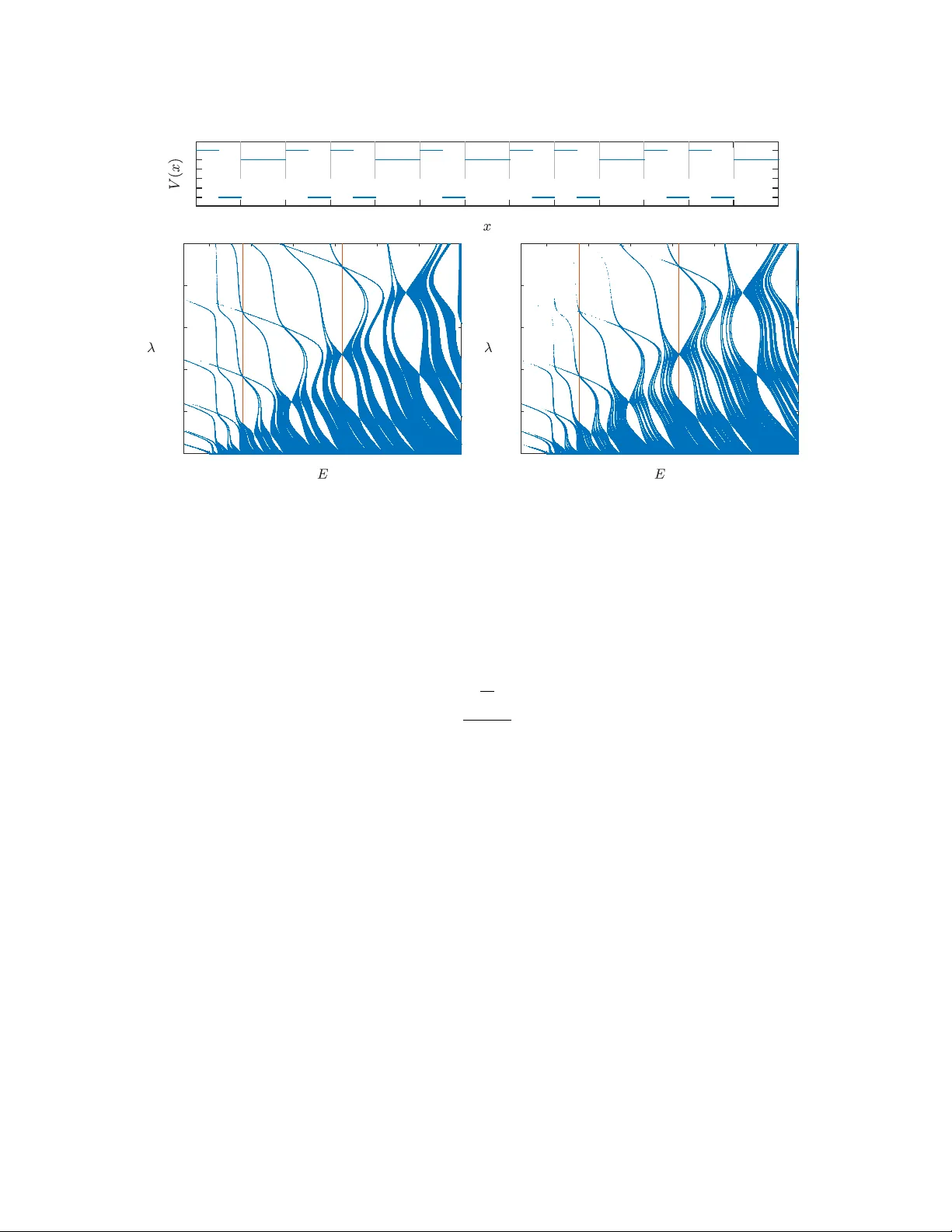
CONTINUUM FIBONA CCI SCHR ¨ ODINGER OPERA TORS IN THE STR ONGL Y COUPLED REGIME D A VID D AMANIK, MARK EMBREE, JAKE FILLMAN, ANTON GORODETSKI, AND MA Y MEI Abstract. W e study Schr¨ odinger op erators on the real line whose p oten tials are generated by the Fib onacci substitution sequence and a rule that replaces symbols b y compactly supp orted p oten tial pieces. W e consider the case in whic h one of those pieces is iden tically zero, and study the dimension of the sp ectrum in the large-coupling regime. Our results include a generalization of theorems regarding explicit examples that w ere studied previously and a counterexample that sho ws that the na ¨ ıv e generalization of previously established statements is false. In par- ticular, in the ap erio dic case, the lo cal Hausdorff dimension of the sp ectrum do es not necessarily con v erge to zero uniformly on compact subsets as the coupling constan t is sent to infinity . 1. Intr oduction 1.1. Main Goals. Since their discov ery in the early 1980s, quasicrystals—structures admitting long-range order sans p erio dicit y—ha ve pla yed a significan t role in materi- als science, ph ysics, and mathematics. The absence of p erio dicit y coupled with long- range order leads to Hamiltonians with exotic sp ectral prop erties, suc h as singular con tin uous sp ectral measures, fractal sp ectrum, and anomalous quantum dynamical transp ort. The Fib onacci substitution sequence has served as a central model of a one- dimensional quasicrystal starting with early w orks in the ph ysics literature such as [ 25 – 27 , 39 ], and follo wed b y a substan tial amount of work in the mathematics literature, including [ 10 , 11 , 13 , 18 – 21 , 43 , 44 ]; see [ 15 , Chapter 10] for more discussion and bac kground ab out the Fib onacci Hamiltonian and [ 2 ] for more background on the mathematics of ap erio dic order. Changing the frequency from the in verse of the golden mean to other irrational n umbers yields other mo dels where the arithmetic prop erties of the con tinued fraction pla y an imp ortan t role [ 23 , 36 , 37 , 47 ]. These works all studied the discr ete tigh t-binding mo del in ℓ 2 ( Z ). Here, w e turn our attention to D.D. was supp orted in part b y National Science F oundation grants DMS–2054752 and DMS– 2349919. M.E. was supp orted in part by National Science F oundation gran t DMS–2411141 and the Simons Institute for the Theory of Computing at UC Berkeley . J. F. was supp orted in part by National Science F oundation gran t DMS–2513006 and b y Simons F oundation gran t MPS TSM–00013720. A.G. was supp orted in part by National Science F oundation grant DMS–2247966. 1 2 D. DAMANIK, M. EMBREE, J. FILLMAN, A. GOR ODETSKI, AND M. MEI the contin uum mo del in L 2 ( R ) given b y [ H V ψ ] = − ψ ′′ + V ψ with V : R → R equiv ariant with resp ect to the Fib onacci sequence. The con tin uum Fib onacci Hamiltonian is exp ected to share many features with the (by no w) very w ell-understo od discrete mo del, although it is considerably more subtle, due to its un b ounded nature and the energy dep endence of the F ric k e–V ogt inv arian t. This class of operators and other related mo dels generated by ap erio dic subshifts were first studied in the 2010s [ 16 , 31 ], but man y important questions remain op en. The w ork [ 16 ] studied the dimension of the sp ectrum for c onstant p oten tial pieces in the regimes of high energy , small coupling, and high coupling. In [ 16 ] the authors ask ed whether the asymptotics for the sp ectral dimension that they derived in the case of constan t p oten tial pieces remain true for general pieces. The results for large energies and small coupling w ere sho wn to hold in complete generalit y (i.e., for arbitrary pieces of p oten tial) [ 22 ], but the large-coupling regime remained elusiv e for the last decade. The main ob jective of this w ork is to show that the asymptotics for high coupling constan t from [ 16 ] do not hold for arbitrary p oten tial pieces, while at the same time giving a partial result under a suitable p ositivit y assumption. As we will see from the argumen ts and examples, the case of large coupling is considerably more delicate in general than the small-coupling and high-energy regimes. Indeed, this is the key c hallenge in the w ork, especially compared to the discrete case, for whic h a more global understanding has b een ac hiev ed [ 21 ]. More sp ecifically , viewing H V = H 0 + V where H 0 = − d 2 / d x 2 , one can recontextualize H λV as a rescaling of λ − 1 H 0 + V . Thus, when λ is large, the co efficien t in front of H 0 is small. In the discrete setting, H 0 is b ounded and hence λ − 1 H 0 + V can b e profitably studied as a p erturbation of V , a diagonal op erator. How ev er, in the present c ontinuum setting, H 0 and therefore λ − 1 H 0 is un b ounded and hence cannot be view ed as a small change to V , regardless of the size of λ . Indeed, it seems that large-coupling asymptotics for con tinuum Sc hr¨ odinger op erators with ergo dic p oten tials are quite delicate in general, 1 though there are a few p ositiv e results suc h as [ 6 , 7 , 42 ]. In fact, one crucial input needed for our w ork w as a study of the large-coupling b eha vior of the Lyapuno v exp onen t and integrated densit y of states (in the guise of the rotation n um b er) for p erio dic contin uum Schr¨ odinger operators, and even those results appear to b e nov el. 1.2. Results. An instance of the Fib onacci substitution sequence can b e written as (1.1) ω n = ⌊ ( n + 1) α + θ ⌋ − ⌊ nα + θ ⌋ , n ∈ Z , where α = ( √ 5 − 1) / 2 denotes the inv erse of the golden mean and θ ∈ R . T o pro duce the related con tin uum mo del, w e choose functions f 0 , f 1 ∈ L 2 ([0 , 1)) and define the resultan t p oten tial by placing a translated copy of f j in [ n, n + 1) whenever ω n = j 1 Indeed, the discrete case is w ell-studied, see, for instance, [ 1 , 35 , 41 , 42 ] for results in that setting. STR ONGL Y COUPLED CONTINUUM FIBONACCI OPERA TORS 3 ( j = 0 , 1). More precisely , w e consider V ω = V f 0 ,f 1 ,ω giv en by (1.2) V ω ( x ) = X n ∈ Z f ω n ( x − n ) , where w e sligh tly abuse notation b y extending f j to v anish outside [0 , 1). One can also construct such p oten tials whenever f 0 and f 1 are defined on in terv als of different lengths via a suitable concatenation pro cedure; this is discussed, for example, in [ 22 , Section 1.2]. W e denote the sp ectrum by Σ = Σ( f 0 , f 1 ), whic h is indep enden t of the choice of θ ∈ T [ 16 ]. In [ 16 ], the authors considered the case of lo cally constant p oten tials f 0 = 0 · χ [0 , 1) and f 1 = 1 · χ [0 , 1) . Abbreviating Σ λ := Σ( λf 0 , λf 1 ), it was shown [ 16 , Corollary 6.6] that for this choice of p oten tial pieces, the lo cal Hausdorff dimension of the sp ectrum satisfies lim λ → 0 inf E ∈ Σ λ dim loc H ( E , Σ λ ) = 1 , (1.3) lim K →∞ inf E ∈ Σ λ ∩ [ K, ∞ ) dim loc H ( E , Σ λ ) = 1 . (1.4) Both of these statemen ts w ere later generalized to an arbitrary pair of functions f 0 , f 1 suc h that the p oten tial given b y ( 1.1 )–( 1.2 ) is ap erio dic 2 [ 22 , Theorems 1.3 and 1.4]. In the case f 0 = 0 · χ [0 , 1) and f 1 = 1 · χ [0 , 1) , one also has (see [ 16 , Corollary 6.7]): (1.5) for any compact S ⊆ R , w e ha v e lim λ →∞ dim H (Σ λ ∩ S ) = 0 . Suc h dimensional statemen ts are quite useful, since they connect to questions of quan tum dynamics [ 30 ] and enable one (generally with even more w ork) to obtain information ab out higher-dimensional mo dels [ 17 ]. The goal of this manuscript is to study whether ( 1.5 ) can be generalized, and under what additional conditions this statemen t could hold. Our first main result sho ws that the natural extension of previous w ork to arbitrary p oten tial pieces is false in a fairly drastic fashion. Let us denote b y C 0 ([0 , 1]) the contin uous functions [0 , 1] → R satisfying f (0) = f (1) = 0 (and note that this pro duces V ω in ( 1.2 ) that are c ontinuous ). Theorem 1.1. Ther e exist f 0  = f 1 ∈ C 0 ([0 , 1]) , E ∈ R , and λ k ↑ ∞ such that (1.6) E ∈ Σ λ k and dim loc H (Σ λ k , E ) = 1 ∀ k . Remark 1.2. (a) Let us reiterate that the assumption f 0  = f 1 implies that the resulting p oten- tials are ap eriodic and hence the conten t of the theorem is non trivial. (b) The term “pseudo band” for the points in a spectrum of zero measure that ha v e full lo cal Hausdorff dimension was suggested in [ 3 ], where the Kronig- –P enney mo del for the Fib onacci potential w as considered; see also [ 28 ] for related results. In this sense the energies describ ed in Theorem 1.1 can b e 2 The statements are trivially true when the resulting p oten tials are p erio dic, i.e., f 1 = f 0 . 4 D. DAMANIK, M. EMBREE, J. FILLMAN, A. GOR ODETSKI, AND M. MEI considered as “pseudo bands” that p ersist for arbitrarily large v alues of the coupling constant. F or any compact set S containing E in its interior, ( 1.6 ) implies dim H (Σ λ k ∩ S ) = 1 for an y k , so, in particular, ( 1.5 ) fails. Nevertheless, a partial result holds under a suitable sign-definiteness assumption. Theorem 1.3. Supp ose f 0 = 0 · χ [0 , 1) , f 1 is c ontinuous and nonne gative, and { x : f 1 ( x ) = 0 } is nowher e dense in [0 , 1] . In this c ase, ( 1.5 ) holds. Figure 1 sho ws the lo w er p ortion of the (unbounded) sp ectrum of p eriodic appro x- imations to tw o contin uum Fib onacci op erators. In b oth cases f 0 = 0 · χ [0 , 1) . On the left, f 1 = 1 · χ [0 , 1) ; on the right f 1 ( x ) = exp(1 + 1 / ((2 x − 1) 2 − 1)), a C ∞ bump function that giv es a contin uous p otential throughout R . (W e discuss the n umerical computations used to create these plots in Section 4 .) Remark 1.4. The case in which the set { f 1 = 0 } contains some in terv als seems to b e more complicated, and if ( 1.5 ) holds in that case, the proof will require some other argumen ts. Indeed, it is not hard to see that in this case the conclusion of Lemma 3.1 no longer holds true for φ = f 1 . W e give the proofs of the main theorems in Section 3 after recalling some back- ground in Section 2 . The construction of a (family of ) counterexamples is quite delicate and requires some surprisingly challenging asymptotics for the Lyapuno v ex- p onen t and rotation num b er for the case of perio dic Sc hro dinger op erators in the large-coupling regime. W e exp ect that the asymptotics work ed out for this pro of ma y b e of interest indep endent of the main results of the curren t w ork. W e need a 0 2 4 6 8 10 12 0 2 4 6 8 10 12 0 2 4 6 8 10 12 0 2 4 6 8 10 12 Figure 1. The low er p ortion of the spectrum for p erio dic approxi- mations (p erio d p = 13) for t wo contin uum Fibonacci op erators with f 0 = 0 · χ [0 , 1) , with f 1 constan t (left) and a C ∞ bump function that is p ositiv e for x ∈ (0 , 1) (right). F or each v alue of λ , the corresp onding sp ectrum is a horizontal slice of the plot. STR ONGL Y COUPLED CONTINUUM FIBONACCI OPERA TORS 5 particular fact about expanding directions of SL(2 , R ) matrices, whic h w e recall in Ap- p endix A . In Section 4 w e briefly review Flo quet theory to characterize the sp ectra of p eriodic appro ximations, and then sho w how, for piecewise constan t p otentials, such sp ectra can b e describ ed as solutions to a parameter-dep enden t, finite-dimensional nonlinear eigenv alue problem. A cknowledgments W e thank the American Institute of Mathematics for their supp ort and hospitality during a recen t SQuaRE meeting, at whic h some of this w ork was done. 2. Ba ckgr ound 2.1. Subshifts. Let A b e a finite set, called the alphab et . Equip A with the discrete top ology and endo w the ful l shift A Z := { ( ω n ) n ∈ Z : ω n ∈ A for all n ∈ Z } with the corresp onding pro duct top ology . The shift [ T ω ] n def = ω n +1 , ω ∈ A Z , n ∈ Z , defines a homeomorphism from A Z to itself. A subset Ω ⊆ A Z is called T -invariant if T − 1 Ω = Ω. An y compact T -in v ariant subset of A Z is called a subshift . W e can asso ciate p otentials (and hence Schr¨ odinger op erators) with elemen ts of subshifts as follows. F or each α ∈ A , w e fix a real-v alued function f α ∈ L 2 ([0 , 1)). Then, for an y ω ∈ A Z , we define the action of the contin uum Schr¨ odinger op erator H ω in L 2 ( R ) by (2.1) H ω = − d 2 d x 2 + V ω , where the p oten tial V ω = V { f α : α ∈A} ,ω is given b y (2.2) V ω ( x ) = X n ∈ Z f ω n ( x − n ) , where, as b efore, f α is extended to v anish outside [0 , 1). These p oten tials b elong to L 2 loc , unif ( R ) and hence eac h H ω defines a self-adjoint op erator on a dense subspace of L 2 ( R ) in a canonical fashion. 2.2. The Fib onacci Subshift. In this pap er, w e study a sp ecial case of the foregoing construction, namely p oten tials generated by elemen ts of the Fib onacci subshift. In this case, the alphab et contains t w o sym b ols, A def = { 0 , 1 } . The Fib onacci substitution is the map S (0) = 1 , S (1) = 10 . This map extends b y concatenation to A ∗ , the free monoid o v er A (i.e., the set of finite words o v er A ), as well as to A N , the collection of (one-sided) infinite words o v er A . There exists a unique element u = 1011010110110 . . . ∈ A N 6 D. DAMANIK, M. EMBREE, J. FILLMAN, A. GOR ODETSKI, AND M. MEI with the prop erty that u = S ( u ). It is straightforw ard to verify that for n ∈ N , S n (1) is a prefix of S n +1 (1). Thus, one obtains u as the limit (in the pro duct top ology on A N ) of the sequence of finite w ords { S n (1) } n ∈ N . The Fib onacci subshift consists of all tw o-sided infinite words with the same lo cal factor structure as u , that is, Ω def = { ω ∈ A Z : ev ery finite subw ord of ω is also a sub w ord of u } . The reader ma y notice that this app ears to b e a different paradigm than the one intro- duced in ( 1.1 ), but rest assured that these t wo definitions are compatible. 3 Giv en real- v alued functions f 0 , f 1 ∈ L 2 ([0 , 1)), w e consider the family of contin uum Sc hr¨ odinger op erators { H ω } ω ∈ Ω defined b y ( 2.1 ) and ( 2.2 ). Since (Ω , T ) is a minimal dynamical system, there is a uniform closed set Σ = Σ( f 0 , f 1 ) ⊆ R with the prop ert y that sp ec( H ω ) = Σ for every ω ∈ Ω . Of course, one can c ho ose f 0 = f 1 , implying that ev ery V ω is a perio dic potential, in whic h case Floquet theory rev eals the sp ectrum to be a union of nondegenerate closed in terv als, and hence, in particular, not no where dense. The main result of [ 16 ] is that p eriodicity of the p oten tials V ω is the only p ossible obstruction to Can tor sp ectrum. W e will later sp ecialize to the case f 0 ≡ 0. In this case, to ensure that eac h V ω is ap eriodic, it suffices to insist that f 1 ≡ 0 in L 2 (i.e., f 1 do es not v anish a.e.). Theorem 2.1 (DFG [ 16 , Corollary 5.5]) . L et Ω denote the Fib onac ci subshift over A = { 0 , 1 } . If the p otential pie c es f 0 and f 1 ar e chosen so that V ω is ap erio dic for one ω ∈ Ω ( henc e for every ω ∈ Ω by minimality ) , then Σ is an extende d Cantor set 4 of zer o L eb esgue me asur e. Let us also inductively define ℓ k > 0 and f k ∈ L 2 ([0 , ℓ k )) by ℓ 0 = ℓ 1 = 1 , ℓ k = ℓ k − 1 + ℓ k − 2 (2.3) f k ( x ) = ( f k − 1 ( x ) , 0 ≤ x < ℓ k − 1 ; f k − 2 ( x − ℓ k − 1 ) , ℓ k − 1 ≤ x < ℓ k . (2.4) 2.3. T race Map, Inv ariant, and Lo cal Dimension of the Spectrum. The sp ec- trum (and many sp ectral characteristics) of the con tinuum Fib onacci mo del can b e enco ded in terms of an asso ciated p olynomial diffeomorphism of R 3 , called the tr ac e map . Let us make this corresp ondence explicit, following [ 16 , 22 ]. T o b egin, w e need to set up some notation. Consider the differential equation (2.5) − y ′′ ( x ) + f ( x ) y ( x ) = E y ( x ) , E ∈ C , x ∈ I , where I ⊆ R is an in terv al and f ∈ L 2 loc ( I ). Giv en a ∈ I , we write u f ,E ,a , v f ,E ,a for the solutions of ( 2.5 ) satisfying the initial conditions (2.6) u f ,E ,a ( a ) = v ′ f ,E ,a ( a ) = 1 and u ′ f ,E ,a ( a ) = v f ,E ,a ( a ) = 0 . 3 The interested reader can consult, for example, [ 15 , Chapter 10] or [ 32 , Chapter 2] for detailed explanations connecting the tw o p erspectives. 4 That is, a closed (but not necessarily compact) p erfect and nowhere dense set. STR ONGL Y COUPLED CONTINUUM FIBONACCI OPERA TORS 7 F or a, b ∈ I , we then define the transfer matrix T [ a,b ] ( f , E ) b y (2.7) T [ a,b ] ( f , E ) def =  v ′ f ,E ,a ( b ) u ′ f ,E ,a ( b ) v f ,E ,a ( b ) u f ,E ,a ( b )  , and note that T [ a,a ] ( f , E ) = I , T [ b,c ] ( f , E ) T [ a,b ] ( f , E ) = T [ a,c ] ( f , E ) (by existence and uniqueness of solutions of ( 2.5 )), and det T [ a,b ] ( f , E ) = 1 for an y a, b, c, f , E . Returning to the Fib onacci setting, we define the mono drom y matrices by M k ( E ) def = T [0 ,ℓ k ] ( f k , E ) , k ∈ Z ≥ 0 , E ∈ C , with ℓ k and f k as in ( 2.3 )–( 2.4 ). Their half-traces are denoted by x k ( E ) def = 1 2 T r( M k ( E )) = 1 2  u f k ,E , 0 ( ℓ k ) + v ′ f k ,E , 0 ( ℓ k )  , k ∈ Z ≥ 0 , E ∈ R . F rom the definitions (and existence and uniqueness of solutions of ( 2.5 )), w e note that M k ( E ) = M k − 2 ( E ) M k − 1 ( E ) , whic h, with the help of the Ca yley–Hamilton theorem, implies (2.8) x k +1 = 2 x k x k − 1 − x k − 2 for all relev ant k . W e can enco de this recursion by a p olynomial map R 3 → R 3 as follo ws: the tr ac e map is defined by T ( x, y , z ) def = (2 xy − z , x, y ) , x, y, z ∈ R , and, in view of ( 2.8 ), one has (2.9) T k ( x 2 , x 1 , x 0 ) = ( x k +2 , x k +1 , x k ) , k ≥ 0 . Th us, the function γ : R → R 3 giv en by γ ( E ) def = ( x 2 ( E ) , x 1 ( E ) , x 0 ( E )) is known as the curve of initial c onditions . The map T is known to hav e a first in tegral given by the so-called F ricke–V o gt invariant , defined b y I ( x, y , z ) def = x 2 + y 2 + z 2 − 2 xy z − 1 , x, y , z ∈ R . More precisely , I ◦ T = I , so T preserves the level surfaces of I : S V def = { ( x, y , z ) ∈ R 3 : I ( x, y , z ) = V } , V ∈ R . Consequen tly , every p oin t of the form T k ( x 2 ( E ) , x 1 ( E ) , x 0 ( E )) with k ∈ Z ≥ 0 lies on the surface S I ( γ ( E )) . F or the sake of conv enience, w e put I ( E ) def = I ( γ ( E )) = I ( x 2 ( E ) , x 1 ( E ) , x 0 ( E )) , with a minor abuse of notation. Putting ev erything together: (2.10) I ( x k +1 ( E ) , x k ( E ) , x k − 1 ( E )) = I ( γ ( E )) for every E and ev ery relev an t k . When V < 0, the set S V has five connected comp onen ts: one compact connected comp onen t that is diffeomorphic to the 2-sphere S 2 , and four unbounded connected 8 D. DAMANIK, M. EMBREE, J. FILLMAN, A. GOR ODETSKI, AND M. MEI comp onen ts, eac h of whic h is diffeomorphic to the op en unit disk. When V = 0, eac h of the four unbounded comp onen ts meets the compact comp onen t, forming four conical singularities. As so on as V > 0, the singularities resolve; for suc h V , the surface S V is smooth, connected, and diffeomorphic to the four-times-punctured 2- sphere. The trace map is imp ortan t in the study of operators of the type ( 2.1 ), as its dynamical sp ectrum, defined by B def =  E ∈ R : { T k ( γ ( E )) : k ∈ Z ≥ 0 } is b ounded  , enco des the op erator-theoretic sp ectrum of H , whic h was first prov ed b y S ¨ ut˝ o in the discrete setting [ 43 ]. Prop osition 2.2 (DF G [ 16 , Prop osition 6.3]) . Σ = B . There are several substantial differences b et w een the contin uum setting and the discrete setting. First, in the discrete case, the F rick e–V ogt in v ariant is constan t (view ed as a function of E , I = I ( E )). Ho wev er, the inv arian t may enjoy nontrivial dep endence on E in the con tinuum setting, whic h is demonstrated by examples in [ 16 ]. This dep endence is related to new phenomena that emerge in the contin uum setting and mak e its study w orthwhile. Moreo v er, w e will show in Prop osition 2.5 that suc h dep endence is an una voidable feature of the contin uum setting: as so on as the p oten tials are ap erio dic, the function I must b e nonconstant. Second, the F rick e–V ogt in v arian t is alwa ys nonnegativ e in the discrete setting (ev en a w a y from the sp ectrum), but one cannot a priori preclude negativity of I in the con tin uum setting. Ho w ev er, it is pro v ed in [ 16 ] that any energies for which I ( E ) < 0 must lie in the resolven t set of the corresp onding con tinuum Fib onacci Hamiltonian. Prop osition 2.3 (DF G [ 16 , Prop osition 6.4]) . F or every E ∈ Σ , one has I ( E ) ≥ 0 . T o study the fractal dimension of the sp ectrum, w e will use the following theorem from [ 16 ], which relates lo cal fractal characteristics near an energy E in the sp ectrum to the v alue of the inv arian t at E . Theorem 2.4 (DF G [ 16 , Theorem 6.5]) . Ther e exists a c ontinuous map D : [0 , ∞ ) → (0 , 1] that is r e al-analytic on R + with the fol lowing pr op erties: (i) dim loc H (Σ; E ) = D ( I ( E )) for e ach E ∈ Σ ; (ii) We have D (0) = 1 and 1 − D ( I ) ∼ √ I as I ↓ 0 ; (iii) We have lim I →∞ D ( I ) · log I = 2 log(1 + √ 2) . Th us, to study the lo cal fractal dimensions of the sp ectrum, it suffices to understand the inv arian t I . Let us return to one of the difficulties men tioned ab o ve: in the curren t setting the in v ariant can in principle b e nonconstan t (as a function of the energy). In fact, not only is it p ossible that I is nonconstant; it is nonconstant if and only if f 0  = f 1 (i.e., the p oten tials V ω are ap erio dic). STR ONGL Y COUPLED CONTINUUM FIBONACCI OPERA TORS 9 Prop osition 2.5. With setup as ab ove, I ( E ) is c onstant if and only if f 0 = f 1 , in which c ase it vanishes identic al ly. Pr o of. With the help of the Ca yley–Hamilton theorem, one can c hec k that (2.11) I ( 1 2 T r A , 1 2 T r B , 1 2 T r AB ) = 1 4 (T r( A − 1 B − 1 AB ) − 2) , A , B ∈ SL(2 , R ) . In particular, for A , B ∈ SL(2 , R ), (2.12) I ( 1 2 T r A , 1 2 T r B , 1 2 T r AB ) = 0 whenev er AB = BA . On one hand, if f 0 = f 1 , then M 0 ( E ) = M 1 ( E ), which certainly commute for every E , leading to I ≡ 0. On the other hand, if I is constan t, then, on accoun t of [ 22 , Section 3], that constant m ust be zero. F rom here, the proof that f 0 = f 1 is similar to and inspired b y the proof of [ 9 , Theorem 2.1]. T o keep this pap er self-contained, we giv e the details. Consider E ∈ R . Due to ( 2.11 ), it follo ws that T r  M 0 ( E ) − 1 M 1 ( E ) − 1 M 0 ( E ) M 1 ( E )  = 2, whic h (since all matrices in question b elong to SL(2 , R )) implies that [ M 0 ( E ) , M 1 ( E )] def = M 0 ( E ) M 1 ( E ) − M 1 ( E ) M 0 ( E ) has a nontrivial kernel and therefore M 0 ( E ) and M 1 ( E ) ha ve at least one common eigen v ector by a standard argument in linear algebra (cf. the pro of of [ 40 , Theo- rem 40.5]). Now, for every E for whic h M 0 is elliptic, its eigenv ectors can b e chosen to b e complex conjugates of one another and hence M 0 ( E ) and M 1 ( E ) are simulta- neously diagonalizable for all such E . Consequen tly , (2.13) M 0 ( E ) M 1 ( E ) − M 1 ( E ) M 0 ( E ) is an analytic function of E that v anishes on a nondegenerate closed interv al, hence v anishes identically . Equiv alen tly , T [0 , 2] ( f 0 ⋆ f 1 , E ) ≡ T [0 , 2] ( f 1 ⋆ f 0 , E ), where we write f 0 ⋆ f 1 for the c onc atenation of f 0 and f 1 (compare ( 2.4 )). By the Borg–Marchenk o theorem (cf. [ 5 , 8 , 34 ]), we ha v e f 0 ⋆ f 1 ≡ f 1 ⋆ f 0 , whence f 0 = f 1 . □ 3. Pr oofs of Main Resul ts Let us b egin with a preparatory result ab out nonnegative p oten tials in the large- coupling regime. In the lemma b elow, w e emphasize that the conclusion holds as long as the p oten tial φ do es not v anish on any nontrivial interv al (how ever, it is otherwise p ermitted to v anish on a set of p ositiv e measure). Lemma 3.1. Supp ose φ : [ a, b ] → [0 , ∞ ) is c ontinuous and { x : φ ( x ) = 0 } is nowher e dense in [ a, b ] . L et M E ,λ = T [ a,b ] ( λφ, E ) b e the mono dr omy matrix r elate d to the e quation (3.1) − y ′′ ( x ) + λφ ( x ) y ( x ) = E y ( x ) , x ∈ [ a, b ] , as define d in ( 2.7 ) . Then for any K ∈ R we have T r M E ,λ → ∞ as λ → ∞ , uniformly in E ≤ K . In p articular, M E ,λ is hyp erb olic for λ lar ge enough. 10 D. DAMANIK, M. EMBREE, J. FILLMAN, A. GOR ODETSKI, AND M. MEI T o prov e Lemma 3.1 , we break some of the main comparison estimates into three further lemmata. Lemma 3.2. Supp ose A ( x ) =  a 11 ( x ) a 12 ( x ) a 21 ( x ) a 22 ( x )  , x ∈ [ a, b ] is a c ontinuous matrix-value d function with nonne gative entries and that B =  b 11 b 12 b 21 b 22  is a c onstant matrix with nonne gative entries satisfying b ij ≤ a ij ( x ) , i, j = 1 , 2 for al l x ∈ [ a, b ] . L et w ∈ R 2 b e a nonzer o ve ctor with w 1 ≥ 0 , w 2 ≥ 0 , and c onsider solutions y and z of the Cauchy pr oblems d y d x = A ( x ) y , d z d x = B z , y ( a ) = z ( a ) = w . Then y i ( x ) ≥ z i ( x ) , i = 1 , 2 , for al l x ∈ [ a, b ] . Pr o of. Consider without loss the case a = 0. Notice that the Cauc h y problem for z is solved b y z ( x ) = e xB w and that the Cauc h y problem for y − z can b e written as d d x ( y − z ) = A ( x )( y − z ) + ( A ( x ) − B ) z , ( y − z )(0) = 0 . By the assumptions on A ( · ), B , and w , it follows that y ( x ) − z ( x ) has nonnegative en tries for all x . □ Lemma 3.3. Supp ose m ≥ 1 and let y ( x ) = [ y 1 y 2 ] ⊤ b e a solution of (3.2)  y ′ 1 y ′ 2  =  0 m 1 0   y 1 y 2  such that y 1 ( a ) ≥ 0 and y 2 ( a ) ≥ 0 . Then, (3.3) d 2 d x 2 ( y 2 1 + y 2 2 ) ≥ 2(1 + m )( y 2 1 + y 2 2 ) . Pr o of. Denote R = y 2 1 + y 2 2 and note from direct computations using ( 3.2 ) that R ′′ = 2  ( y ′ 1 ) 2 + y 1 y ′′ 1 + ( y ′ 2 ) 2 + y 2 y ′′ 2 )  = 2  m 2 y 2 2 + my 2 1 + y 2 1 + my 2 2  ≥ 2(1 + m )( y 2 1 + y 2 2 ) , (3.4) as promised. □ Lemma 3.4. Supp ose k > 0 and R ( x ) , x ∈ [ a, b ] , is a C 2 -function such that (3.5)        R ′′ ≥ k R, R ′ ≥ 0 , R ( a ) = R 0 > 0 . Then R ( x ) ≥ R 0 2  e √ k ( x − a ) + e − √ k ( x − a )  for al l x ∈ [ a, b ] . STR ONGL Y COUPLED CONTINUUM FIBONACCI OPERA TORS 11 Pr o of. F or a small ε > 0, consider a related system S ′′ = k S with initial conditions S ( a ) = R 0 − ε > 0 and S ′ ( a ) = 0. Then we hav e S ( x ) = R 0 − ε 2  e √ k ( x − a ) + e − √ k ( x − a )  . If T ( x ) = R ( x ) − S ( x ), then w e hav e T ′′ ≥ k T , T ′ ( a ) ≥ 0, T ( a ) = ε > 0, from whic h w e see that T ( x ) ≥ ε > 0 for all x ∈ [ a, b ]. Therefore, R ( x ) ≥ R 0 − ε 2  e √ k ( x − a ) + e − √ k ( x − a )  . Since ε > 0 can b e taken arbitrarily small, this implies the desired estimate. □ W e no w use these results to prov e the first main technical lemma. Pr o of of L emma 3.1 . Consider the nonautonomous flow on R 2 giv en by (3.6) d d x  y 1 y 2  =  0 λφ ( x ) − E 1 0   y 1 y 2  , and notice that y solves ( 3.1 ) if and only if ( y ′ , y ) ⊤ solv es ( 3.6 ). Then the Dirichlet solution (that is, the solution that satisfies y ( a ) = 0, y ′ ( a ) = 1) corresp onds to the dynamics of the vector (1 , 0) ⊤ , and the Neumann solution ( y ( a ) = 1, y ′ ( a ) = 0) corresp onds to the dynamics of the vector (0 , 1) ⊤ . F or an y vector u = ( u 1 , u 2 ) ⊤ ∈ R 2 , and an y x 1 < x 2 from [ a, b ], denote by (3.7) F [ x 1 ,x 2 ] ( u ) def = T [ x 1 ,x 2 ] ( λφ, E ) u ∈ R 2 the solution of ( 3.6 ) at the moment x 2 , for initial conditions y 1 ( x 1 ) = u 1 , y 2 ( x 1 ) = u 2 . F or t ∈ ( − π / 2 , π / 2), define the cone V t def = n v ∈ R 2 \ { 0 } : arg v ∈  0 , π 2 + t o . Fix s > 0 small. W e will split the pro of into sev eral claims. Claim 1. There exists ε = ε ( φ, K, s ) > 0 such that for any E ≤ K and any λ ≥ 0, the following hold: (a) F or an y v ector w ∈ V 0 and an y [ x 1 , x 2 ] ⊆ [ a, b ] with | x 2 − x 1 | ≤ ε , one has F [ x 1 ,x 2 ] ( w ) ∈ V s . (b) F or an y vector w ∈ V − s and any [ x 1 , x 2 ] ⊆ [ a, b ] with | x 2 − x 1 | ≤ ε , one has F [ x 1 ,x 2 ] ( w ) ∈ V 0 . (c) In b oth settings, | F [ x 1 ,x 2 ] ( w ) | > 1 2 | w | . Pro of of Claim. Assume without loss that K ≥ 1. Consider w ∈ V 0 and the solu- tion y = ( y 1 , y 2 ) ⊤ of ( 3.6 ) with y ( x 1 ) = w . W rite y ( x ) = ( y 1 ( x ) , y 2 ( x )) ⊤ in p olar co ordinates as (3.8) y 1 ( x ) = r ( x ) cos θ ( x ) , y 2 ( x ) = r ( x ) sin θ ( x ) , 12 D. DAMANIK, M. EMBREE, J. FILLMAN, A. GOR ODETSKI, AND M. MEI with r ≥ 0 and θ c hosen contin uously in x with θ ( x 1 ) ∈ (0 , π / 2). Note that d θ d x = y 1 y ′ 2 − y ′ 1 y 2 y 2 1 + y 2 2 = y 2 1 − ( λφ − E ) y 2 2 y 2 1 + y 2 2 = cos 2 θ − ( λφ − E ) sin 2 θ . (3.9) By the choice of K , θ ′ ( x ) ≤ K uniformly in x . Consequently , if | x 2 − x 1 | ≤ ε ≤ s/ (2 K ), arg F [ x 1 ,x 2 ] ( w ) = θ ( x 2 ) ≤ arg w + K ε < arg w + s. Moreo v er, ( 3.9 ) also implies that θ ′ ( x ) > 0 if θ ( x ) > 0 is small enough. Putting these t w o observ ations together shows that an y ε > 0 with ε ≤ s/ (2 K ) satisfies (a) and (b). T o address part (c), first observe that d r d x = 1 r ( y 1 y ′ 1 + y 2 y ′ 2 ) = r cos θ sin θ ( λφ − E + 1) . (3.10) Th us, for an y x for which θ ( x ) ∈ [0 , π / 2], one has (3.11) d d x log r = 1 r d r d x ≥ − K . T o deal with the case θ ( x ) ∈ ( π / 2 , π / 2 + s ), notice first that com bining ( 3.9 ) and ( 3.10 ) gives 1 cos θ sin θ 1 r d r d x = λφ − E + 1 = 1 sin 2 θ − 1 sin 2 θ d θ d x , and thus 1 r d r d x = − cos θ sin θ d θ d x + cos θ sin θ . Denote the set of x ∈ ( x 1 , x 2 ) with θ ( x ) > π / 2 by S ( a i , b i ) ≡ S I i . W e ha ve Z b i a i 1 r d r d x d x = − Z b i a i cos θ sin θ d θ d x d x + Z b i a i cos θ sin θ d x ≥ − Z θ ( b i ) θ ( a i ) cos θ sin θ d θ − | I i |    cot  π 2 + s     . F or an y I i with θ ( a i ) = θ ( b i ), the first term drops out. Otherwise, that first term is nonnegativ e, so one arrives at Z b i a i 1 r d r d x d x ≥ −| I i |    cot  π 2 + s     ≥ − 3 s | I i | (3.12) for small enough s > 0. Com bining ( 3.11 ) with ( 3.12 ) pro duces the desired result. ♢ Claim 2. F or an y ε > 0, there exists a partition of the in terv al [ a, b ], t 0 = a < t 1 < t 2 < · · · < t N − 1 < t N = b, suc h that (a) F or ev ery i , one has | t i +1 − t i | < ε ; (b) If φ ( t ) = 0 for some t ∈ ( t i , t i +1 ), then φ > 0 throughout any in terv al of the partition that is adjacent to [ t i , t i +1 ]. STR ONGL Y COUPLED CONTINUUM FIBONACCI OPERA TORS 13 Pro of of Claim. Choose a partition a = s 0 < · · · < s M = b of [ a, b ] in to interv als of length at most ε/ 2. Then, for eac h j = 1 , 2 , . . . , M , the assumption that φ − 1 ( { 0 } ) is no where dense permits us to c ho ose a nondegenerate in terv al [ t 2 j − 1 , t 2 j ] ⊆ ( s j − 1 , s j ) on whic h φ is positive, yielding the desired { t i } after putting t 0 = a , N = 2 M + 1, and t N = b . ♢ Claim 3. If an interv al [ x 1 , x 2 ] ⊆ [ a, b ] is such that φ > 0 throughout [ x 1 , x 2 ], then there exists λ 0 = λ 0 ( x 1 , x 2 , φ, K , s ) suc h that for any λ ≥ λ 0 and any w ∈ V s , we ha ve F [ x 1 ,x 2 ] ( w ) ∈ V − s . Moreov er, | F [ x 1 ,x 2 ] ( w ) | ≥ 1 2 | w | as λ → + ∞ . Pro of of Claim. Fix C = C ( x 1 , x 2 , s ) > 0 large enough that (3.13) sin 2 (2 s ) − C cos 2 (2 s ) < − 4 s ( x 2 − x 1 ) − 1 . Since φ is contin uous, w e may then c ho ose λ 0 > 0 large enough that λφ ( x ) − E ≥ C throughout [ x 1 , x 2 ] for all λ ≥ λ 0 . F or any x ∈ [ x 1 , x 2 ] for whic h | θ ( x ) − π / 2 | < 2 s , ( 3.9 ) then yields (3.14) d θ d x = cos 2 θ − ( λφ − E ) sin 2 θ ≤ sin 2 (2 s ) − C cos 2 (2 s ) < − 4 s ( x 2 − x 1 ) − 1 . Using ( 3.14 ) shows that for an y w ∈ V s \ V − s , one has arg F [ x 1 ,x 2 ] ( w ) < π 2 − s . Recalling that θ ′ > 0 when θ > 0 is small, this prov es the first part of the claim. Let us no w justify the second part of the claim. Supp ose w ∈ V s \ V − s (otherwise there is nothing to pro ve, since r ( x ) is increasing if θ ( x ) ∈ (0 , π / 2) and λ is large; see ( 3.10 )). F rom ( 3.9 ) and ( 3.10 ) we ha v e, for θ ∈  π 2 − s, π 2 + s  and λ sufficiently large,     d r d θ     =     r cos θ sin θ ( λφ − E + 1) cos 2 θ − ( λφ − E ) sin 2 θ     ≤ r | cos θ |    cos 2 θ 1+ λφ − E − λφ − E 1+ λφ − E sin 2 θ    ≤ 2 r | cos θ | . Hence, if w ∈ V s \ V − s , then     d d θ log r     ≤ 2 | cos θ | ≤ 2    θ − π 2    ≤ 2 s. Set r 0 = | w | and r 1 = | F [ x 1 ,x ∗ ] ( w ) | , where x ∗ ∈ [ x 1 , x 2 ] is suc h that θ ( x ∗ ) = π 2 − s . Then we ha ve log r 1 ≥ log r 0 − 4 s 2 , and r 1 ≥ e − 4 s 2 r 0 ≥ 1 2 r 0 , since s is small. Since r ( x ) is increasing for θ ( x ) ∈  0 , π 2  , this implies that | F [ x 1 ,x 2 ] ( w ) | ≥ 1 2 | w | . ♢ Claim 4. If an interv al [ x 1 , x 2 ] ⊆ [ a, b ] is such that φ ( x ) > 0 for all x ∈ [ x 1 , x 2 ], then for any w ∈ V 0 , we ha v e | F [ x 1 ,x 2 ] ( w ) | → + ∞ as λ → + ∞ uniformly in E ≤ K . Pro of of Claim. This claim follo ws from applying Lemmas 3.2 , 3.3 , and 3.4 to ( 3.6 ) with the initial conditions given b y the v ector w . ♢ T aken together, these claims imply that the mono drom y matrix M E ,λ can b e rep- resen ted as a pro duct of matrices such that after an application of the first one or tw o matrices in this pro duct, the image of each of the unit co ordinate v ectors will b e in the first quadrant, remain there afterwards, and their images can b e made arbitrarily large by c ho osing a sufficien tly large v alue of λ . This implies that T r M E ,λ → ∞ as λ → ∞ , uniformly in E ≤ K . □ 14 D. DAMANIK, M. EMBREE, J. FILLMAN, A. GOR ODETSKI, AND M. MEI With Lemma 3.1 , we are now able to prov e Theorem 1.3 . Pr o of of The or em 1.3 . Fix S ⊆ R compact, and denote A = M 0 and B = M 1 . Notice that A is indep enden t of λ , and if the v alue of the energy E is restricted to a fixed compact set S , then A is uniformly b ounded: there exists M = M ( S ) > 1 suc h that ∥ A ( E ) ∥ ≤ M for every E ∈ S . Pic k K ≫ M > 1 sufficien tly large. On account of Lemma 3.1 , we kno w that | T r( B ( E , λ )) | > 2 K for all E ∈ S when λ is large enough. W e no w consider t wo cases. Case 1: | T r(AB) | > 2 K 1 / 3 . Then, w e hav e | x 2 | =     1 2 T r( AB )     > K 1 / 3 , | x 1 | =     1 2 T r( B )     > K , | x 0 | =     1 2 T r( A )     ≤ M , with K ≫ M . It follows that the corresponding energy E has an un b ounded trace orbit (pro vided that K is large enough) b y standard arguments (e.g., [ 15 , Theo- rem 10.5.4]) and hence is not in the sp ectrum on accoun t of Prop osition 2.2 . Case 2: | T r(AB) | ≤ 2 K 1 / 3 . Defining { x k } as b efore, w e hav e | x 2 | =     1 2 T r( AB )     ≤ K 1 / 3 , | x 1 | =     1 2 T r( B )     > K , | x 0 | =     1 2 T r( A )     ≤ M , w e can b ound the v alue of the F rick e–V ogt inv ariant: I = x 2 0 + x 2 1 + x 2 2 − 2 x 0 x 1 x 2 − 1 ≳ K 2 . Therefore, if E ∈ S belongs to the sp ectrum, the lo cal Hausdorff dimension at E can b e estimated from ab o ve via Theorem 2.4 , and the upp er b ound on the Hausdorff dimension tends to zero as λ → ∞ , since K → ∞ as λ → ∞ . □ W e no w turn to the pro of of Theorem 1.1 . W e will in fact show that C 1 functions that alternate from p ositiv e to negativ e supply a family of counterexamples. Definition 3.5. Let us sa y that f ∈ C 1 ([0 , 1]) is a split function if f (0) = f (1) = 0 and there exists x ∗ ∈ (0 , 1) such that (1) f ( x ) > 0 for 0 < x < x ∗ ; (2) f ( x ) < 0 for x ∗ < x < 1; (3) f ′ ( x ∗ ) < 0 and f ′ (1) > 0. Notice that these assumptions force f ( x ∗ ) = 0. Theorem 3.6. Supp ose f 0 = 0 · χ [0 , 1) and f 1 ∈ C 1 ([0 , 1]) is a split function. Then, ther e exist E ∈ R , λ k ↑ ∞ such that E ∈ Σ λ k := Σ( λ k f 0 , λ k f 1 ) and (3.15) dim loc H (Σ λ k , E ) = 1 for al l k . Remark 3.7. W e suspect that Theorem 3.6 still holds if assumption (3) in the defini- tion of the split function is remo v ed, but most lik ely a different argument is required. STR ONGL Y COUPLED CONTINUUM FIBONACCI OPERA TORS 15 W riting a solution to the nonautonomous flo w ( 3.6 ) in p olar co ordinates as in the pro of of Lemma 3.1 , and introducing L = log r , ( 3.9 ) and ( 3.10 ) can b e rewritten as (3.16)        d θ d x = 1 − ( λφ − E + 1) sin 2 θ , d L d x = cos θ sin θ ( λφ − E + 1) . Let us consider the solutions of this system separately on the interv als (0 , x ∗ ) and ( x ∗ , 1). The arguments that follo w inv olve v arious constan ts that ma y dep end on f and E , but which m ust b e indep enden t of λ . W e write f ≲ g if f ≤ C g for suc h a constan t C , and f ≍ g if b oth f ≲ g and g ≲ f . Here w e emphasize that the (ev entual) applications of Lemmata 3.8 – 3.13 b elo w will b e for a fixed energy , so ha ving energy-dep enden t constants is not problematic for the applications that we ha v e in mind. Lemma 3.8. Assume that φ is c ontinuous on [ a, b ] and strictly p ositive on ( a, b ) , and fix E ∈ R . Then L ( b ) − L ( a ) ≳ √ λ , wher e L ( x ) is any solution of the system ( 3.16 ) with θ ( a ) ∈ (0 , π / 2) . Pr o of. Without loss of generalit y , consider L ( a ) = 0. The assumption θ ( a ) ∈ (0 , π / 2) giv es y ( a ) , y ′ ( a ) > 0. Let us consider first the case in whic h φ is strictly p ositiv e on [ a, b ]. By assumption we can choose C 2 > C 1 > 0 suc h that for all λ large enough, w e hav e for all x ∈ [ a, b ], C 1 λ < λφ ( x ) − E + 1 < C 2 λ. Note that for such λ , an y zero of the right hand side of the first equation of ( 3.16 ), θ ∗ ( x ), must ob ey (3.17) 1 sin 2 θ ∗ ( x ) = λφ ( x ) − E + 1 ∈ ( C 1 λ, C 2 λ ) . W e c ho ose θ ∗ ( a ) ∈ (0 , π / 2) and then con tinuously choose θ ∗ on ( a, b ). In view of ( 3.17 ), w e note that there are constants C ′ 2 > C ′ 1 > 0 such that for all x and λ under consideration: (3.18) θ ∗ ( x ) ∈  C ′ 1 √ λ , C ′ 2 √ λ  . W e also observe that θ ′ ( x ) > 0 (resp., < 0) if sin 2 θ ( x ) < sin 2 θ ∗ ( x ) (resp., sin 2 θ ( x ) > sin 2 θ ∗ ( x ).) In particular, θ ( x ) remains in (0 , π / 2) for all x , so the result follows directly by applying Lemma 3.4 to the function R = y (and noting that L ≥ log y ). No w consider the case in which φ v anishes at one or more endp oints by noting first that ( 3.16 ) implies that θ ′ = 1 when θ = 0 and θ ′ ≤ E + 1 everywhere, so since θ ( a ) ∈ (0 , π / 2), we may fix ε > 0 small enough to ensure that θ ( a + ε ) ∈ (0 , π / 2) (the smallness condition dep ends on E , which is fixed for this argument). W e may then apply the argumen t from the previous case on [ a + ε, b − ε ] to obtain L ( b − ε ) − L ( a + ε ) ≳ √ λ. 16 D. DAMANIK, M. EMBREE, J. FILLMAN, A. GOR ODETSKI, AND M. MEI On the b oundary in terv als, we ha v e L ′ ≥ − E , so the total c hange in L is (3.19) L ( b ) − L ( a ) ≳ √ λ − 2 E ε ≳ √ λ, where we p ermit an E -dep enden t constant in the final estimate. □ Let us no w study what happ ens on an interv al on which φ ≤ 0. Lemma 3.9. Assume that φ is c ontinuous and strictly ne gative on ( c, d ) and that E > 0 . If θ denotes a solution of ( 3.16 ) , then (3.20) θ ( d ) − θ ( c ) ≍ √ λ for lar ge λ. Pr o of. Consider first the case when φ is strictly negativ e throughout [ c, d ]. Since φ is strictly negative and b ounded a wa y from zero, one can c ho ose C > 0 such that λφ ( x ) − E + 1 ≤ − C λ for all sufficiently large λ . In view of ( 3.16 ), one has (3.21) d θ d x = 1 − ( λφ − E + 1) sin 2 θ ≥ 1 + C λ sin 2 θ . In particular, the map x 7→ θ ( x ) can b e inv erted. Thus, viewing x as a function of θ and changing v ariables, we hav e d − c = Z d c d x = Z θ ( d ) θ ( c ) d θ 1 − ( λφ ( x ( θ )) − E + 1) sin 2 θ ≤ Z θ ( d ) θ ( c ) d θ 1 + C λ sin 2 θ = 1 C λ Z θ ( d ) θ ( c ) d θ sin 2 θ + 1 C λ . Since R π 0 d θ sin 2 θ + a 2 = π a √ 1+ a 2 , using π -p eriodicity of the integrand, we obtain the low er b ound in ( 3.20 ). A completely analogous pro of establishes the upp er b ound in ( 3.20 ), noting that the boundedness of φ allows us to estimate λφ ( x ) − E + 1 ≥ − e C λ for e C > 0 and λ sufficiently large. No w consider the case in which φ v anishes at one or more endp oints. Fixing ε > 0, w e may apply the previous argument on [ c + ε, d − ε ] ⊆ ( c, d ) to obtain (3.22) θ ( d − ε ) − θ ( c + ε ) ≍ √ λ. On the b oundary interv als, w e notice that w e still ha v e d θ / d x ≥ E sin 2 θ ≥ 0 and the one-sided b ound λφ − E + 1 ≥ − e C λ for a suitable e C > 0, which enables us to reprise the previous argumen t to deduce 0 ≤ θ ( c + ε ) − θ ( c ) ≲ √ λ and a similar statemen t on the other b oundary interv al, whic h suffices to derive the desired b ounds. □ STR ONGL Y COUPLED CONTINUUM FIBONACCI OPERA TORS 17 The final task is to estimate the asymptotics of L on [ x ∗ , 1], the interv al of non- p ositivit y . This is the most delicate part of the analysis, whic h we break in to yet smaller steps. Without loss of generality , we can assume min φ = − 1. W e will then break [ x ∗ , 1] in to three regimes: for w ell-chosen 0 < ε 1 < ε 2 < 1, we will consider the micr osc opic ( − λ ε 1 ≤ λφ ≤ 0), mesosc opic ( − λ ε 2 ≤ λφ ≤ − λ ε 1 ), and macr osc opic ( − λ ≤ λφ ≤ − λ − ε 2 ) regions. One further technical p oin t merits attention here: the in terv als defining the v arious regimes are themselves dependent on λ , so to appro- priately track the λ -dep endence, we must incorp orate the length of the interv als into some of the estimates b elow. Lemma 3.10. Assume that φ is c ontinuously differ entiable and strictly ne gative on [ c, d ] and that E > 0 . If L ( x ) is a solution of ( 3.16 ) then | L ( d ) − L ( c ) | ≲ log λ as λ → ∞ . Pr o of. Notice that ( 3.16 ) implies (3.23) d L d θ = cos θ sin θ − 1 E − λφ ( x ( θ )) − 1 − sin 2 θ , where w e use monotonicit y to view x as a function of θ as in the pro of of Lemma 3.9 ; th us, our goal is to change v ariables and use (3.24) L ( d ) − L ( c ) = Z θ ( d ) θ ( c ) d L d θ d θ . As b efore, we can assume that λ is large enough that λφ ( x ) − E + 1 ≤ − C λ for all x and λ under consideration. As in the pro of of Lemma 3.9 , using (3.25) d x d θ = 1 1 − ( λφ − E + 1) sin 2 θ ≤ 1 1 + C λ sin 2 θ , w e see that on an y θ interv al of the form [ π n, π ( n + 1)], x can c hange b y no more than ≲ λ − 1 / 2 . Under the given assumptions, φ ( x ) is Lipsc hitz contin uous. Due to Lemma 3.9 , θ is changing o v er some interv al [ θ ( c ) , θ ( d )], where θ ( d ) − θ ( c ) ≍ √ λ . Let us split that in terv al into sub-interv als of length π . Notice that if φ were constant, the in tegral of the righ t hand side of ( 3.23 ) ov er [ π n, π ( n + 1)] would be zero (since the denominator is symmetric with resp ect to the center of the in terv al [ π n, π ( n + 1)], and the numerator is anti-symmetric). By Lipschitz con tin uit y of φ we ha v e max [ π n,π ( n +1)] φ ( x ( θ )) − min [ π n,π ( n +1)] φ ( x ( θ )) ≲ 1 √ λ . If | φ ( x ( θ )) − φ ( x ( θ 0 )) | ≲ λ − 1 / 2 , then − 1 E − λφ ( x ( θ )) − 1 is equal to − 1 E − λφ ( x ( θ 0 )) − 1 up to a correction of order at most λ − 3 / 2 . Therefore, since Z π ( n +1) π n cos θ sin θ − 1 E − λφ ( x ( θ 0 )) − 1 − sin 2 θ d θ = 0 , 18 D. DAMANIK, M. EMBREE, J. FILLMAN, A. GOR ODETSKI, AND M. MEI w e claim that the in tegral Z π ( n +1) π n cos θ sin θ − 1 E − λφ ( x ( θ )) − 1 − sin 2 θ d θ has order at most λ − 1 / 2 . Indeed, w e hav e      Z π ( n +1) π n cos θ sin θ − 1 E − λφ ( x ( θ )) − 1 − sin 2 θ d θ      =      Z π ( n +1) π n cos θ sin θ − 1 E − λφ ( x ( θ )) − 1 − sin 2 θ d θ − Z π ( n +1) π n cos θ sin θ − 1 E − λφ ( x ( θ 0 )) − 1 − sin 2 θ d θ      ≲ 1 λ 3 / 2 Z π ( n +1) π n | cos θ sin θ | ( a 2 + sin 2 θ ) 2 d θ , where a 2 = min θ ∈ [ π n,π ( n +1)] 1 E − λφ ( x ( θ )) − 1 ≍ 1 λ . Using Z π / 2 0 cos θ sin θ ( a 2 + sin 2 θ ) 2 d θ = 1 2 a 2 ( a 2 + 1) , w e get (3.26)      Z π ( n +1) π n cos θ sin θ − 1 E − λφ ( x ( θ )) − 1 − sin 2 θ d θ      ≲ 1 √ λ . Since θ ( d ) − θ ( c ) ≍ √ λ , in the case in which the in terv al [ θ ( c ) , θ ( d )] splits in to a union of in terv als of the form [ π n, π ( n + 1)], the integral Z θ ( d ) θ ( c ) cos θ sin θ − 1 E − λφ ( x ( θ )) − 1 − sin 2 θ d θ is at most of order √ λ · 1 √ λ = 1. A t last, it remains to b ound the integral R J cos θ sin θ − 1 E − λφ ( x ( θ )) − 1 − sin 2 θ d θ ov er an interv al J of length smaller than π . Since the n umerator is an tisymmetric ab out p oin ts of the form π ( n + 1 2 ) and the denominator do es not change sign, the integral in question is b ounded from ab o v e by the absolute v alue of an integral of the form Z J ′ cos θ sin θ − 1 E − λφ ( x ( θ )) − 1 − sin 2 θ d θ , where J ′ is of the form [ πn, π ( n + 1 / 2)] or [ π ( n + 1 / 2) , π ( n + 1)] for an in teger n . Since R π / 2 0 cos( x ) sin( x ) a 2 +sin 2 ( x ) d x = 1 2 ln  1 + 1 a 2  , this implies that     R J ′ cos θ sin θ − 1 E − λφ ( x ( θ )) − 1 − sin 2 θ d θ     ≲ log λ, whic h completes the pro of of the lemma. □ Let us now treat the case when the function φ is negative in the in terior of an in terv al, but v anishes at the b oundary p oints. STR ONGL Y COUPLED CONTINUUM FIBONACCI OPERA TORS 19 Lemma 3.11. Assume that φ is c ontinuously differ entiable on [ c, d ] , strictly ne gative on ( c, d ) , e qual to zer o at the end p oints c and d , φ ′ ( c ) < 0 and φ ′ ( d ) > 0 , and that E > 0 . If L ( x ) is a solution of ( 3.16 ) , then for lar ge enough values of λ we have | L ( d ) − L ( c ) | ≲ λ 9 20 . W e will need a few statements to prov e Lemma 3.11 . Lemma 3.12. Supp ose that on the interval [ c, d ] for some ε > 0 we have − λ ε − 1 ≤ φ ≤ 0 , and let L ( x ) b e a solution of ( 3.16 ) . Then for lar ge λ we have | L ( d ) − L ( c ) | ≲ λ ε ( d − c ) . Pr o of. Without loss, consider L ( c ) = 0. F or λ is large, one has | λφ − E + 1 | ≲ C λ ε . Therefore, the solution of the equation L ′ = cos θ sin θ ( λφ − E + 1) cannot grow faster than the solution of the equation e L ′ = C λ ε . □ Lemma 3.13. Supp ose that on the interval [ c, d ] we have − λ ε 2 − 1 ≤ φ ≤ − λ ε 1 − 1 for some 0 < ε 1 < ε 2 ≤ 1 , and let L ( x ) b e a solution of ( 3.16 ) with the initial c ondition L ( c ) = 0 . Then for lar ge λ we have | L ( d ) | ≲ ( d − c ) λ 1+ 3 2 ε 2 − 5 2 ε 1 + log λ. Pr o of. Let J π denote an in terv al of length π . W e ha v e (3.27) d x d θ = 1 1 − ( λφ − E + 1) sin 2 θ ≤ 1 C λ ε 1 sin 2 θ + 1 , and since R J π d θ sin 2 θ + a 2 = π a √ 1+ a 2 , on the interv al J π the v alue of x = x ( θ ) changes by at most (3.28) Z J π d x d θ d θ ≲ λ − ε 1 2 . T ogether with Lipschitz con tin uit y of φ , this implies that max x ∈ J π φ ( x ( θ )) − min x ∈ J π φ ( x ( θ )) ≲ λ − ε 1 2 . Hence, for an y θ , θ 0 ∈ J π w e hav e     1 E − λφ ( x ( θ )) − 1 − 1 E − λφ ( x ( θ 0 )) − 1     ≲ λ · λ − ε 1 / 2 λ 2 ε 1 = λ 1 − 5 ε 1 2 . 20 D. DAMANIK, M. EMBREE, J. FILLMAN, A. GOR ODETSKI, AND M. MEI Therefore, rep eating the argument from the pro of of Lemma 3.10 , we get, for any θ 0 ∈ J π , that      Z J π cos θ sin θ − 1 E − λφ ( x ( θ )) − 1 − sin 2 θ d θ      =      Z J π cos θ sin θ − 1 E − λφ ( x ( θ )) − 1 − sin 2 θ d θ − Z J π cos θ sin θ − 1 E − λφ ( x ( θ 0 )) − 1 − sin 2 θ d θ      ≲ λ 1 − 5 ε 1 2 Z J π | cos θ sin θ | ( a 2 + sin 2 θ ) 2 d θ , where a 2 = min θ ∈ J π 1 E − λφ ( x ( θ )) − 1 ≥ 1 E + λ ε 2 − 1 ≳ 1 λ ε 2 . Since R π / 2 0 cos x sin x ( a 2 +sin 2 x ) 2 d x = 1 2 a 2 ( a 2 +1) , we ha v e      Z J π cos θ sin θ − 1 E − λφ ( x ( θ )) − 1 − sin 2 θ d θ      ≲ λ 1 − 5 ε 1 2 · λ ε 2 = λ 1+ ε 2 − 5 ε 1 2 . No w, we claim that θ ( d ) − θ ( c ) ≲ max(1 , ( d − c ) λ ε 2 / 2 ) . Indeed, for large λ we ha ve d θ d x = 1 − ( λφ − E + 1) sin 2 θ ≤ 1 + 2 λ ε 2 sin 2 θ , hence d − c = Z d c d x = Z θ ( d ) θ ( c ) d θ 1 − ( λφ ( x ( θ )) − E + 1) sin 2 θ ≥ Z θ ( d ) θ ( c ) d θ 1 + 2 λ ε 2 sin 2 θ = 1 2 λ ε 2 Z θ ( d ) θ ( c ) d θ 1 2 λ ε 2 + sin 2 θ . If θ ( d ) − θ ( c ) > π , then, taking into accoun t that R π 0 d θ sin 2 θ + a 2 = π a √ 1+ a 2 , we ha v e d − c ≥ 1 2 λ ε 2 Z θ ( d ) θ ( c ) d θ 1 2 λ ε 2 + sin 2 θ ≥ 1 2 λ ε 2  θ ( d ) − θ ( c ) π − 1  Z π 0 d θ 1 2 λ ε 2 + sin 2 θ ≳ λ − ε 2 / 2  θ ( d ) − θ ( c ) π − 1  , so θ ( d ) − θ ( c ) ≲ ( d − c ) λ ε 2 / 2 + 1. Incorp orating also the case in whic h θ ( d ) − θ ( c ) ≤ π , w e get θ ( d ) − θ ( c ) ≲ max(1 , ( d − c ) λ ε 2 / 2 ) . Therefore, if the interv al [ θ ( c ) , θ ( d )] splits in to interv als of length π exactly , w e ha v e | L ( d ) | ≲ ( d − c ) λ ε 2 / 2 λ 1+ ε 2 − 5 ε 1 2 = ( d − c ) λ 1+ 3 2 ε 2 − 5 2 ε 1 . STR ONGL Y COUPLED CONTINUUM FIBONACCI OPERA TORS 21 Finally , if the in terv al [ θ ( c ) , θ ( d )] do es not split into in terv als of length π exactly , w e can get a remainder of order log λ in this estimate, as was sho wn in the pro of of Lemma 3.10 . This completes the pro of of the lemma. □ No w are ready to pro ve Lemma 3.11 . Pr o of of L emma 3.11 . Fix ε 1 = 29 40 and ε 2 = 33 40 , let φ denote a function satisfying the assumptions of the lemma; w e may assume without loss that min φ = − 1. Since φ ′ ( c ) < 0 and φ ∈ C 1 , there exists δ > 0 such that φ ′ < 0 and hence φ is decreasing on [ c, c + δ ]. It follows that for any sufficiently large λ > 0, the in terv al  c, c + d 2  can b e split into the union [ c 1 , d 1 ] ∪ [ c 2 , d 2 ] ∪ [ c 3 , d 3 ] of in terv als with disjoint interior, so that c = c 1 , d 1 = c 2 , d 2 = c 3 , d 3 = c + d 2 , and the follo wing hold: (1) − λ ε 1 − 1 ≤ φ ≤ 0 if x ∈ [ c 1 , d 1 ]; (2) − λ ε 2 − 1 ≤ φ ≤ − λ ε 1 − 1 if x ∈ [ c 2 , d 2 ]; (3) − 1 ≤ φ ≤ − λ ε 2 − 1 if x ∈ [ c 3 , d 3 ]. F or large λ > 0 w e hav e d 1 − c 1 ≍ λ ε 1 − 1 , d 2 − c 2 ≍ λ ε 2 − 1 , d 3 − c 3 ≍ 1 . Applying Lemma 3.12 on [ c 1 , d 1 ] and Lemma 3.13 t wice (once as written on [ c 2 , d 2 ] and a second time with ( ε 1 , ε 2 ) replaced b y ( ε 2 , 1) on [ c 3 , d 3 ]), we obtain L ( d 1 ) − L ( c 1 ) ≲ λ 2 ε 1 − 1 , L ( d 2 ) − L ( c 2 ) ≲ λ 5 ε 2 2 − 5 ε 1 2 , L ( d 3 ) − L ( c 3 ) ≲ λ 5 − 5 ε 2 2 . In particular, for our choice of the v alues of ε 1 , ε 2 w e hav e 2 ε 1 − 1 = 9 20 , 5 ε 2 2 − 5 ε 1 2 = 1 4 < 9 20 , 5 − 5 ε 2 2 = 35 80 < 9 20 . Therefore, L ( d 3 ) − L ( c 1 ) ≲ λ 9 20 . Application of an analogous argument to the in terv al  c + d 2 , d  completes the pro of. □ Pr o of of The or em 3.6 . Fix E of the form E = 4 π 2 n 2 , denote A = M 0 , B = M 1 , and define (3.29) B 1 ( E , λ ) def = T [0 ,x ∗ ] ( λf 1 , E ) , B 2 ( E , λ ) def = T [ x ∗ , 1] ( λf 1 , E ) . Since A = I , it suffices to sho w that w e can c ho ose λ k → ∞ such that B = B ( E , λ k ) = B 2 ( E , λ k ) B 1 ( E , λ k ) satisfies B 2 = − I . Indeed, this would imply that B is elliptic and therefore E b elongs to the sp ectrum. F urthermore, since A = I , it follo ws that A and B commute, and therefore I ( E ) = 0, so that the lo cal Hausdorff dimension of the sp ectrum at E is one. T o that end, we note that log ∥ B 1 ∥ ≳ λ 1 / 2 b y Lemma 3.8 . By the pro of of Lemma 3.8 and Prop osition A.1 , the expanding direction of B 1 , U ( B 1 ), satisfies (3.30) ∠ ( B 1 U ( B 1 ) , e 1 ) ≲ exp( − λ 1 / 2 ) , 22 D. DAMANIK, M. EMBREE, J. FILLMAN, A. GOR ODETSKI, AND M. MEI where e 1 = (1 , 0) ⊤ . By Lemma 3.11 , log ∥ B 2 ∥ ≲ λ 9 / 20 , so log ∥ B ∥ ≳ λ 1 / 2 − λ 9 / 20 ≳ λ 1 / 2 with B 1 U ( B ) ≈ (1 , 0) ⊤ as w ell. Then, by taking adv antage of Lemma 3.9 , we can start at an y large λ v alue that we lik e and increase until w e arrive at a λ for which (3.31) B U ( B ) = B 2 B 1 U ( B ) = S ( B ) . Since B U ( B ) = S ( B − 1 ) is orthogonal to U ( B − 1 ) = B S ( B ), it follo ws that B ex- c hanges the subspaces { U ( B ) , S ( B ) } , so T r B = 0, which implies B 2 = − I by the Ca yley–Hamilton theorem, concluding the argumen t. □ 4. A Nonlinear Eigenv alue F ormula tion 4.1. A V ery Brief Review of Flo quet Theory. Supp ose V : R → R is p -p erio dic with p > 0 and (4.1) Z p 0 | V ( x ) | 2 d x < ∞ . Let us recall a few notions from Flo quet theory . F or pro ofs, see [ 33 , Chapter 11]; for additional background and context, see [ 29 ]. T o study the sp ectral prop erties of L V = − ∂ 2 x + V , consider the follo wing family of boundary v alue problems, indexed b y a parameter ϑ ∈ [0 , π ]: (4.2) − y ′′ ( x ) + V ( x ) y ( x ) = E y ( x ) , y ( p ) = e iϑ y (0) , y ′ ( p ) = e iϑ y ′ (0) . F or eac h E and ϑ , the solution space of ( 4.2 ) can b e 0-, 1-, or 2-dimensional. F or a giv en V , p , and ϑ ∈ [0 , π ], write E 1 ( ϑ ; V , p ) ≤ E 2 ( ϑ ; V , p ) ≤ · · · for the sp ectrum of ( 4.2 ), that is, the list of E ∈ R (with m ultiplicit y) suc h that ( 4.2 ) has a non trivial solution. W e ha v e the following facts: • Each E j ( · ; V , p ) is monotonic on [0 , π ]. In fact, E j is incr e asing if j is odd and de cr e asing if j is even. • The sp ectrum of L V is given b y (4.3) sp ec( L V ) = { E j ( ϑ ; V , p ) : ϑ ∈ [0 , π ] , j ≥ 1 } . Com bining these t wo p oints, (4.4) sp ec( L V ) = ∞ [ j =1  [ E 2 j − 1 (0) , E 2 j − 1 ( π )] ∪ [ E 2 j ( π ) , E 2 j (0)]  . In particular, to iden tify the sp ectrum of L V , it suffices to identify the p oin ts E j ( ϑ ) with ϑ ∈ { 0 , π } and furthermore, one has (4.5) sp ec( L V ) = { E ∈ R : T r T [0 ,p ] ( V , E ) ∈ [ − 2 , 2] } . STR ONGL Y COUPLED CONTINUUM FIBONACCI OPERA TORS 23 4.2. A Nonlinear Eigen v alue Problem for Periodic Approximations. W e no w return to the Fib onacci setting. When f 0 and f 1 p ermit an exact solution form ula for − y ′′ ( x ) + λf j ( x ) y ( x ) = E y ( x ), the Flo quet c haracterization of the sp ectrum of p eriodic appro ximations to the con tinuum Fib onacci op erator can b e c haracterized b y a parameterized nonlinear eigen v alue problem. This approach resem bles the frame- w ork prop osed b y Mennick en and M¨ oller, e.g., with application to serially connected b eams [ 38 , Sect. 10.4] and netw orks of strings [ 4 ], as w ell as the Wittrick–Williams metho d of dynamic stiffness matrices [ 46 ]. W e first consider the constan t p oten tials f 0 = 0 · χ [0 , 1) and f 1 = λ · χ [0 , 1) in the case of k = 2, i.e., p eriod p = 2. Let y 1 , y 2 : [0 , 1] → C denote the solutions of ( 2.5 ) on the sub domains [0 , 1] and [1 , 2]. 5 F or the given p oten tial, equation ( 2.5 ) requires (4.6) − y ′′ 1 ( x ) + λy 1 ( x ) = E y 1 ( x ) , − y ′′ 2 ( x ) = E y 2 ( x ) . These constant-coefficient equations ha ve the general solutions (for E  = λ ) y 1 ( x ) = A 1 sin( √ E − λ x ) + B 1 cos( √ E − λ x ) y 2 ( x ) = A 2 sin( √ E x ) + B 2 cos( √ E x ) . A t the sub domain in terface, con tinuit y and smo othness ( y 1 (1) = y 2 (0), y ′ 1 (1) = y ′ 2 (0)) require A 1 sin( √ E − λ ) + B 1 cos( √ E − λ ) = B 2 A 1 √ E − λ cos( √ E − λ ) − B 1 √ E − λ sin( √ E − λ ) = A 2 √ E . A t the ends of the domain, the Flo quet conditions ( 4.2 ) require y 2 (1) = e iϑ y 1 (0) and y ′ 2 (1) = e iϑ y ′ 1 (0), giving A 2 sin( √ E ) + B 2 cos( √ E ) = B 1 e iϑ A 2 √ E cos( √ E ) − B 2 √ E sin( √ E ) = A 1 e iϑ √ E − λ. Arrange these last four equations into the standard form       sin( √ E − λ ) cos( √ E − λ ) 0 − 1 √ E − λ cos( √ E − λ ) − √ E − λ sin( √ E − λ ) − √ E 0 0 − e iϑ sin( √ E ) cos( √ E ) − e iϑ √ E − λ 0 √ E cos( √ E ) − √ E sin( √ E )             A 1 B 1 A 2 B 2       =       0 0 0 0       . W e seek v alues of E for which the matrix on the left, T λ,ϑ ( E ), is singular (and the corresp onding solution of the differen tial equation is nontrivial ). There will generally b e infinitely many such real v alues of E . A wide range of algorithms exist for finding these eigen v alues; see, e.g., G ¨ uttel and Tisseur [ 24 ]. (Indeed, this family of examples could provide useful test problems for these algorithms.) This p eriod-2 case can b e readily generalized to p erio d p = F k , where F k is the k th Fibonacci num b er ( F 0 = F 1 = 1, F k +1 = F k + F k − 1 ). Let { ω n } n ∈ Z denote the 5 In the second case, we translate the argument so that y 2 is a function on [0 , 1], not [1 , 2]. 24 D. DAMANIK, M. EMBREE, J. FILLMAN, A. GOR ODETSKI, AND M. MEI 0 1 2 3 4 5 6 7 8 9 10 11 12 13 -4 -3 -2 -1 0 1 0 50 100 150 200 250 300 0 50 100 150 200 250 0 50 100 150 200 250 300 0 50 100 150 200 250 Figure 2. F or the piecewise constant p otential with c = 4 (sho wn on the top), the b ottom plots sho w a p ortion of the sp ectrum for p eriodic appro ximations ( p = F 4 = 5, left; p = F 6 = 13, righ t). The vertical red lines indicate the v alues of E = 4 π 2 and E = 16 π 2 . sequence of p erio d F k determined from ( 1.1 ) but with α replaced by α k := F k /F k +1 (and θ = 0). In tro duce φ n ( E ) = ( √ E , ω n = 0; √ E − λ, ω n = 1 . Let e j ∈ C 2 F k denote the j th column of the identit y matrix. Then we can express the nonlinear eigenv alue function as T λ,ϑ ( E ) : C 2 F k → C 2 F k as T λ,ϑ ( E ) = F k X n =1  sin( φ n ( E )) e 2 n − 1 e ⊤ 2 n − 1 + cos( φ n ( E )) e 2 n − 1 e ⊤ 2 n  + F k X n =1  φ n ( E ) cos( φ n ( E )) e 2 n e ⊤ 2 n − 1 − φ n ( E ) sin( φ n ( E )) e 2 n e ⊤ 2 n  − F k − 1 X n =1 e 2 n − 1 e ⊤ 2 n +2 − F k − 1 X n =1 φ n +1 ( E ) e 2 n e ⊤ 2 n +1 − e iϑ e 2 F k − 1 e ⊤ 2 − φ 1 ( E ) e iϑ e 2 F k e ⊤ 1 . STR ONGL Y COUPLED CONTINUUM FIBONACCI OPERA TORS 25 38 38.5 39 39.5 40 40.5 91.0 91.5 92.0 92.5 93.0 93.5 38 38.5 39 39.5 40 40.5 91.0 91.5 92.0 92.5 93.0 93.5 Figure 3. F or the potential in Figure 2 , no w fo cusing on the sp ec- trum near E = 4 π 2 (v ertical red line) and the first λ > E for whic h T r B ( E , λ ) = 0 (horizontal red line), for p eriodic appro ximations ( p = F 4 = 5, left; p = F 6 = 13, righ t). W e observ e F 3 = 3 and F 5 = 8 bands in these plots. Motiv ated b y Theorem 3.6 , w e consider f 0 = 0 · χ [0 , 1) and f 1 a simple discrete v ersion of a split function: (4.7) f 1 ( x ) = ( 1 0 ≤ x < 1 / 2 − c 1 / 2 ≤ x < 1 , where c > 0 is a suitable constan t. Of course, f 1 is not C 1 and hence not a genuine split function, but we remark in passing that the arguments pro ving Theorem 3.6 can b e adjusted to apply to this c hoice of f 1 , which thus gives us a useful b enc hmark for the computations. Since this p oten tial is constant on each sub domain [ j / 2 , ( j + 1) / 2] for j ∈ Z , w e can apply the approach just describ ed to c haracterize the spectra of p eriodic approximations. In this case, it is conv enient (if sligh tly profligate) to solve the differential equation on half-unit sub domains, so that the order p = F k p eriodic appro ximation leads to a nonlinear eigenv alue problem of order 4 F k (rather than 2 F k , as previously). This formulation can b e used to study the fine sp ectral structure for suitable potentials. F or example, Figure 2 sho ws a portion of the spectrum for p eriodic approximations of length p = F 5 = 8 and p = F 6 = 13 for c = 4. There exists an un b ounded sequence { λ k } suc h that E = 4 π 2 is in the sp ectrum Σ k . T o in v estigate this phenomenon, Figure 3 fo cuses around E = 4 π 2 and the first v alue of λ > E suc h that B ( E , λ ) = 0; the red lines show λ = 92 . 46773 and E = 4 π 2 . (These later plots resem ble the sp ectra of p erio dic appro ximations to discr ete Fib onacci op erators [ 12 , Fig. 4].) In Figure 4 we replace the piecewise constant f 1 b y the b ona fide split function f 1 ( x ) = 50 x ( x − 1 / 3)( x − 1) . W e observ e similar sp ectral features, as exp ected from Theorem 3.6 . 26 D. DAMANIK, M. EMBREE, J. FILLMAN, A. GOR ODETSKI, AND M. MEI 0 1 2 3 4 5 6 7 8 9 10 11 12 13 -4 -3 -2 -1 0 1 -50 0 50 100 150 200 250 300 0 50 100 150 200 250 37.5 38 38.5 39 39.5 40 40.5 41 41.5 169.0 169.5 170.0 170.5 171.0 171.5 172.0 172.5 173.0 173.5 Figure 4. F or a smo oth p oten tial inv olving a split function f 1 (sho wn on the top), the b ottom plots show a portion of the sp ectrum for the p eriodic approximation with p = F 4 = 5 (left), and a zo om for p = F 6 = 13 (righ t) showing a confluence of F 5 = 8 sp ectral bands around E = 4 π 2 (v ertical red line). F or n umerical in vestigations, w e complement this nonlinear eigenv alue formula- tion with a piecewise Cheb yshev pseudosp ectral discretization [ 45 ] of the differen tial equations. This approach, which w e used to create all the plots in this pap er, has the adv an tage of allo wing p otentials that are not piecewise constan t, as in the left plot in Figure 1 and in Figure 4 . The nonlinear eigen v alue formulation pro vides a wa y to b enc hmark the accuracy of the discretization metho d using examples with piecewise constan t p oten tials. Appendix A. Singular Vectors of Hyperbolic Ma trices W e need the follo wing elementary statement ab out expanding directions and ex- panding eigenspaces for hyperb olic SL(2 , R ) matrices. Here we recall that any A ∈ SL(2 , R ) with ∥ A ∥ > 1 has expanding and contracting directions U ( A ) , S ( A ) ∈ RP 1 suc h that (A.1) | A u | = ∥ A ∥ , | A s | = ∥ A ∥ − 1 for any unit v ectors u ∈ U ( A ), s ∈ S ( A ). Prop osition A.1. Supp ose A ∈ SL(2 , R ) is hyp erb olic with eigenvalues λ ± 1 , wher e | λ | > 1 . L et U ( A ) denote the dir e ction that is most exp ande d by A and V ( A ) the STR ONGL Y COUPLED CONTINUUM FIBONACCI OPERA TORS 27 eigensp ac e with eigenvalue λ . Then, (A.2) ∠ ( V ( A ) , A U ( A )) ≤ π 2 | λ |∥ A ∥ . Pr o of. F or an y unit v ector v ∈ V ( A ), we hav e (A.3)   A − 1 v   = | λ | − 1 . Th us, applying [ 14 , Prop osition 1.13.5] to A − 1 with R = | λ | − 1 and using ∥ A − 1 ∥ = ∥ A ∥ , one obtains ∠ ( V ( A ) , A U ( A )) = ∠ ( V ( A ) , S ( A − 1 )) ≤ π 2 | λ |∥ A ∥ , as promised. □ References [1] J. Avron, W. Craig, and B. Simon. Large coupling behaviour of the Lyapuno v exp onen t for tigh t binding one-dimensional random systems. J. Phys. A: Math. Gen. , 16(7):L209–L211, 1983. [2] M. Baake and U. Grimm. Ap erio dic Or der. Vol. 1 , v olume 149 of Encyclop e dia of Mathematics and its Applic ations . Cambridge Universit y Press, Cambridge, 2013. [3] M. Baake, D. Joseph, and P . Kramer. Periodic clustering in the sp ectrum of quasiperio dic Kronig–Penney mo dels. Phys. L ett. A , 168(3):199–208, 1992. [4] J. P . Baker. Vibr ations of me chanic al structur es: sour c e lo c alization and nonline ar eigenvalue pr oblems for mo de c alculation . PhD thesis, Virginia T ec h, 2023. [5] C. Bennewitz. A pro of of the lo cal Borg–March enko theorem. Comm. Math. Phys. , 218:131–132, 2001. [6] K. Bjerkl¨ ov. Positiv e Lyapuno v exp onen ts for contin uous quasip eriodic Schr¨ odinger equations. J. Math. Ph ys. , 47(2):022702, 4, 2006. [7] K. Bjerkl¨ ov. P ositive Lyapuno v exp onen t and minimalit y for the contin uous 1-d quasi-p erio dic Sc hr¨ odinger equations with tw o basic frequencies. Ann. Henri Poinc ar´ e , 8(4):687–730, 2007. [8] G. Borg. Uniqueness theorems in the spectral theory of y ′′ + ( λ − q ( x )) y = 0. In Den 11te Skandinaviske Matematikerkongr ess, Tr ondheim, 1949 , pages 276–287. Johan Grundt T an ums F orlag, Oslo, 1952. [9] V. Buca j, D. Damanik, J. Fillman, V. Gerbuz, T. V andenBo om, F. W ang, and Z. Zhang. P ositive Lyapuno v exponents and a large deviation theorem for contin uum Anderson mo dels, briefly . J. F unct. Anal. , 277(9):3179–3186, 2019. [10] S. Cantat. Bers and H´ enon, Painlev´ e and Schr¨ odinger. Duke Math. J. , 149(3):411–460, 2009. [11] M. Casdagli. Symbolic dynamics for the renormalization map of a quasip erio dic Schr¨ odinger equation. Comm. Math. Phys. , 107(2):295–318, 1986. [12] D. Damanik, M. Em bree, and A. Goro detski. Sp ectral prop erties of Sc hr¨ odinger op erators arising in the study of quasicrystals. In J. Kellendonk, D. Lenz, and J. Savinien, editors, Math- ematics of Ap erio dic Or der , pages 307–370. Birkh¨ auser, Basel, 2015. [13] D. Damanik, M. Em bree, A. Goro detski, and S. Tcheremc han tsev. The fractal dimension of the sp ectrum of the Fib onacci Hamiltonian. Comm. Math. Phys. , 280(2):499–516, 2008. [14] D. Damanik and J. Fillman. One-Dimensional Er go dic Schr¨ odinger Op er ators—I. Gener al The- ory , v olume 221 of Gr aduate Studies in Mathematics . American Mathematical So ciet y , Provi- dence, RI, 2022. [15] D. Damanik and J. Fillman. One-Dimensional Er go dic Schr¨ odinger Op er ators—II. Sp e cific Classes , v olume 249 of Gr aduate Studies in Mathematics . American Mathematical So ciet y , Pro vidence, RI, 2024. 28 D. DAMANIK, M. EMBREE, J. FILLMAN, A. GOR ODETSKI, AND M. MEI [16] D. Damanik, J. Fillman, and A. Goro detski. Con tin uum Sc hr¨ odinger op erators asso ciated with ap eriodic subshifts. Ann. Henri Poinc ar´ e , 15(6):1123–1144, 2014. [17] D. Damanik, J. Fillman, and A. Goro detski. Multidimensional Schr¨ odinger op erators whose sp ectrum features a half-line and a Cantor set. J. F unct. Anal. , 280(7):P ap er No. 108911, 38, 2021. [18] D. Damanik and A. Gorodetski. Spectral and quan tum dynamical prop erties of the weakly coupled Fib onacci Hamiltonian. Comm. Math. Phys. , 305(1):221–277, 2011. [19] D. Damanik and A. Goro detski. The density of states measure of the w eakly coupled Fibonacci Hamiltonian. Ge om. F unct. Anal. , 22(4):976–989, 2012. [20] D. Damanik and A. Goro detski. H¨ older contin uity of the in tegrated density of states for the Fib onacci Hamiltonian. Comm. Math. Phys. , 323(2):497–515, 2013. [21] D. Damanik, A. Goro detski, and W. Y essen. The Fibonacci Hamiltonian. Invent. Math. , 206(3):629–692, 2016. [22] J. Fillman and M. Mei. Sp ectral prop erties of con tin uum Fibonacci Sc hr¨ odinger op erators. A nn. Henri Poinc ar ´ e , 19(1):237–247, 2018. [23] A. Girand. Dynamical Green functions and discrete Schr¨ odinger operators with p oten tials gen- erated by primitiv e inv ertible substitution. Nonline arity , 27(3):527–543, 2014. [24] S. G ¨ uttel and F. Tisseur. The nonlinear eigen v alue problem. A cta Numeric a , pages 1–94, 2017. [25] M. Kohmoto. Dynamical system related to quasip erio dic Schr¨ odinger equations in one dimen- sion. J. Statist. Phys. , 66:791–796, 1992. [26] M. Kohmoto, L. P . Kadanoff, and C. T ang. Localization problem in one dimension: mapping and escap e. Phys. R ev. L ett. , 50(23):1870–1872, 1983. [27] M. Kohmoto, B. Sutherland, and C. T ang. Critical w av e functions and a Can tor-set sp ectrum of a one-dimensional quasicrystal mo del. Phys. R ev. B (3) , 35(3):1020–1033, 1987. [28] J. Koll´ ar and A. S ¨ ut˜ o. The Kronig–Penney mo del on a Fib onacci lattice. Physics L etters A , 117(4):203–209, 1986. [29] P . Kuc hmen t. An o verview of perio dic elliptic operators. Bul l. Amer. Math. So c. (N.S.) , 53(3):343–414, 2016. [30] Y. Last. Quantum dynamics and decomp ositions of singular con tinuous sp ectra. J. F unct. A nal. , 142(2):406–445, 1996. [31] D. Lenz, C. Seifert, and P . Stollmann. Zero measure Cantor sp ectra for con tin uum one- dimensional quasicrystals. J. Differ. Equ. , 256(6):1905–1926, 2014. [32] M. Lothaire. Algebr aic Combinatorics on Wor ds , volume 90 of Encyclop e dia of Mathematics and its Applic ations . Cambridge Universit y Press, Cambridge, 2002. [33] M. Luki´ c. A First Course in Sp e ctr al The ory , volume 226 of Gr aduate Studies in Mathematics . American Mathematical So ciet y , 2022. [34] V. A. Marchenk o. Concerning the theory of a differen tial operator of the second order. Doklady A kad. Nauk SSSR (N.S.) , 72:457–460, 1950. [35] F. Martinelli and L. Mic heli. On the large-coupling-constan t behavior of the Liapuno v exp onen t in a binary alloy . J. Statist. Phys. , 48(1–2):1–18, 1987. [36] M. Mei. Sp ectra of discrete Schr¨ odinger op erators with primitive inv ertible substitution poten- tials. J. Math. Phys. , 55(8):082701, 22, 2014. [37] M. Mei and W. Y essen. T ridiagonal substitution Hamiltonians. Math. Mo del. Nat. Phenom. , 9(5):204–238, 2014. [38] R. Mennic ken and M. M¨ oller. Non-Self-A djoint Boundary Eigenvalue Pr oblems . Elsevier, Am- sterdam, 2003. [39] S. Ostlund, R. Pandit, D. Rand, H. J. Sc hellnh ub er, and E. D. Siggia. One-dimensional Sc hr¨ odinger equation with an almost p erio dic p oten tial. Phys. R ev. L ett. , 50(23):1873–1876, 1983. STR ONGL Y COUPLED CONTINUUM FIBONACCI OPERA TORS 29 [40] V. V. Prasolov. Pr oblems and The or ems in Line ar Algebr a , v olume 134 of T r anslations of Math- ematic al Mono gr aphs . American Mathematical So ciet y , Providence, RI, 1994. T ranslated from the Russian man uscript b y D. A. Le ˘ ites. [41] M. Shamis and T. Sp encer. Bounds on the Ly apuno v exponent via crude estimates on the densit y of states. Comm. Math. Phys. , 338(2):705–720, 2015. [42] E. Sorets and T. Sp encer. Positiv e Ly apunov exp onen ts for Schr¨ odinger op erators with quasi- p eriodic p otentials. Comm. Math. Phys. , 142(3):543–566, 1991. [43] A. S ¨ ut˝ o. Singular contin uous sp ectrum on a Can tor set of zero Leb esgue measure for the Fi- b onacci Hamiltonian. J. Statist. Phys. , 56(3–4):525–531, 1989. [44] A. S ¨ ut˝ o. The sp ectrum of a quasiperio dic Sc hr¨ odinger operator. Comm. Math. Phys. , 111(3):409–415, 1987. [45] L. N. T refethen. Sp e ctr al Metho ds in MA TLAB . SIAM, Philadelphia, 2000. [46] W. H. Wittrick and F. W. Williams. A general algorithm for computing natural frequencies of elastic structures. Quart. J. Me ch. Appl. Math. , 24:263–284, 1971. [47] W. N. Y essen. Sp ectral analysis of tridiagonal Fib onacci Hamiltonians. J. Sp e ctr. The ory , 3(1):101–128, 2013. Dep ar tment of Ma thema tics, Rice University, 6100 S. Main Street, Houston, Texas 77005-1892, USA Email addr ess : damanik@rice.edu Dep ar tment of Ma thema tics, Virginia Tech, Blacksburg, V A 24061, USA Email addr ess : embree@vt.edu Dep ar tment of Ma thema tics, Texas A&M University, College St a tion, TX 77843, USA Email addr ess : fillman@tamu.edu Dep ar tment of Ma thema tics, University of California, Ir vine, CA 92697, USA Email addr ess : asgor@uci.edu Dep ar tment of Ma thema tics, Denison University, Granville, OH 43023, USA Email addr ess : meim@denison.edu